practice and theory of opinion mining and sentiment analysis · with sentiment analysis or opinion...
TRANSCRIPT
Volume 29 — Number 1 — 2014 — ISSN 2190-6858
Journal for Language Technology
and Computational Linguistics
Practice and Theory of
Opinion Mining and
Sentiment Analysis
Herausgegeben von/Edited by
Michael Wiegand, Robert Remus und Stefan Gindl
Gesellschaft für Sprachtechnologie & Computerlinguistik

Contents
EditorialStefan Gindl, Robert Remus, Michael Wiegand . iii
Unsupervised feature learning for sentiment classifica-tion of short documentsSimone Albertini, Alessandro Zamberletti, IgnazioGallo . . . . . . . . . . . . . . . . . . . . . . . . . 1
Domain Adaptation for Opinion Mining: A Study ofMultipolarity WordsMorgane Marchand, Romaric Besancon, OlivierMesnard, Anne Vilnat . . . . . . . . . . . . . . . 17
IGGSA-STEPS: Shared Task on Source and TargetExtraction from Political SpeechesJosef Ruppenhofer, Julia Maria Struß, JonathanSonntag, Stefan Gindl . . . . . . . . . . . . . . . 33
Subjectivity Lexicon for Czech: Implementation andImprovementsKaterina Veselovska, Jan Hajic, jr., Jana Sindlerova 47
The notion of importance in academic writing: detec-tion, linguistic properties and targetsStefania Degaetano-Ortlieb, Hannah Kermes, ElkeTeich . . . . . . . . . . . . . . . . . . . . . . . . 63
Using Brain Data for Sentiment AnalysisYuqiao Gu, Fabio Celli, Josef Steinberger, An-drew James Anderson, Massimo Poesio, CarloStrapparava, Brian Murphy . . . . . . . . . . . . 79
Author Index . . . . . . . . . . . . . . . . . . . . . . . 95

Impressum
Herausgeber Gesellschaft fur Sprachtechnologie undComputerlinguistik (GSCL)
Aktuelle Ausgabe Band 29 – 2014 – Heft 1Gastherausgeber Michael Wiegand, Robert Remus,
Stefan GindlAnschrift der Redaktion Lothar Lemnitzer
Berlin-Brandenburgische Akademie derWissenschaftenJagerstr. 22/2310117 [email protected]
ISSN 2190-6858Erscheinungsweise 2 Hefte im Jahr,
Publikation nur elektronischOnline-Prasenz www.jlcl.org

iii
Editorial
The abundance of opinions available on the World Wide Web represents an information
repository of enormous intellectual and economic value. Automated methods to exploit this
rich knowledge mine have become more and more relevant within the last decade and the
availability of large amounts of data is an ideal premise for the application of empirical
methods.
Although many researchers from different nations and institutes intensively work on the
development of these techniques, many challenges have been left uncovered. The most
pressing problems range from migrating sentiment analysis systems to new text types or
domains, developing robust natural language applications that effectively exploit sentiment
analysis, to the creation of resources that enable research in other languages than English.
Moreover, a deeper understanding of subjective language beyond lexical keyword matching
still needs to be acquired.
This special issue consists of a selection of papers presented at the 2nd Workshop on
Practice and Theory of Opinion Mining and Sentiment Analysis (PATHOS) held in conjunc-
tion with GSCL-2013 in Darmstadt, Germany, on September 23rd, 2013. In order to ensure
articles of a high quality, a second reviewing cycle was carried out on the revised submis-
sions originally accepted and presented at the PATHOS workshop.
We briefly outline the topics addressed in those papers:
Albertini et al. present an unsupervised method based on Growing Hierarchical
Self-Organizing Maps to provide an alternative feature encoding. The aim of this
encoding is to obtain a less sparse feature representation that typically arises with
(traditional) bag of words applied on short documents. In the light of the growing
importance of analyzing short texts from microblogging services, most prominent-
ly messages from Twitter, the task addressed by the authors is highly relevant to
sentiment analysis. Their proposed encoding is evaluated against other competing
methods (such as Autoencoders) and shown to outperform them.
Another paper that focuses on learning-based methods is Marchand et al. who ex-
amine multi-polarity words, i.e. polar expressions that change their polarity across
different domains. As the set of domains on which sentiment analysis can be ap-
plied is pretty large, learning-based approaches often face the problem that only
labeled out-of-domain training data are available. Marchand et al. show that the
deletion of multi-polarity words substantially improves classification performance
when such training data are used and propose a method to detect such words. They
assume a realistic setting in which no labeled information from the target domain
is available.

iv
Ruppenhofer et al. describe the shared task on source and target extraction from
political speeches which is to be organized in summer 2014. This article makes a
welcome contribution to JLCL, being the flagship journal for research in German
speaking countries, since it describes the first shared task that is exclusively con-
cerned with sentiment analysis in German.
Another work that focuses on sentiment analysis on a language other than English
is presented by Veselovska et al. who introduce a subjectivity lexicon for Czech.
The work describes the creation of the resource and its evaluation on polarity clas-
sification in four different domains and is an important example of resource crea-
tion for Czech.
Degaetano-Ortlieb et al. report on a study in a rather different direction. It is a de-
scriptive approach on sentiment analysis whose purpose is to uncover evaluative
expressions with a focus on the notion of "importance" in the genre of scientific
research articles. The study is carried out on a specially annotated corpus that al-
lows an examination of very complex linguistic properties. We believe that such
research enables a deeper understanding of sentiment and subjective language than
can be gained by the predominant resources, such as textual corpora labeled for
polarity and sentiment lexicons.
The last article of this issue comes in a similar vein. Gu et al. present an explorato-
ry study of using electroencephalography (EEG) for the prediction of lexical va-
lence. This is a highly interdisciplinary work as it departs from traditional uni-
modal approaches of sentiment analysis that exclusively draw information for pre-
diction from text. This work is an example of the emerging research area of multi-
modal analysis that has recently attracted wide attention in sentiment analysis.
We would like to thank the “Gesellschaft für Sprachtechnologie und Computerlinguistik”
for accepting this volume to be published in the JLCL series. Special thanks also go to
Thierry Declerck, the editor-in-chief of the journal, for supporting us with technical issues in
creating this special issue. Moreover, we are indebted to our reviewers for their hard work.
Last but not least, we thank the authors of the articles for their interesting contributions.
August 2014
Stefan Gindl, Robert Remus, Michael Wiegand


Simone Albertini, Alessandro Zamberletti, Ignazio Gallo
Unsupervised feature learning for sentiment classification ofshort documents
Abstract
The rapid growth of Web information led to an increasing amount of user-generatedcontent, such as customer reviews of products, forum posts and blogs. In this paper weface the task of assigning a sentiment polarity to user-generated short documents todetermine whether each of them communicates a positive or negative judgment abouta subject. The method we propose exploits a Growing Hierarchical Self-OrganizingMap as feature learning algorithm to obtain a sparse encoding of the input data. Theencoded documents are subsequently given as input to a Support Vector Machineclassifier that assigns them a polarity label. Unlike other works on opinion mining, ourmodel does not exploit a priori hypotheses involving special words, phrases or languageconstructs typical of certain domains. Using a dataset composed by customer reviewsof products, our experimental results prove that the proposed method can overcomeother state-of-the-art feature learning approaches.
1 Introduction
E-commerce has grown significantly over the past decade. As such, there has been aproliferation of reviews written by customers for different products and those reviewsare of great value for the businesses as they convey a lot of information both aboutsellers and products e.g. the overall customers’ satisfaction.With sentiment analysis or opinion mining we refer to the task of assigning a
sentiment polarity to text documents to determine whether the reviewer expressed apositive, neutral or negative judgment about a subject (Pang and Lee, 2008). This isan interesting and useful task that has been successfully applied to several differentsources of information, e.g., movies (Zhuang et al., 2006) and product reviews (Hu andLiu, 2004; Popescu and Etzioni, 2005; Ding et al., 2008) to name a few.Many works in literature (Kanayama and Nasukawa, 2006; Wen and Wu, 2011;
Ku et al., 2011) manage to build lexicons of opinion-bearing words or phrases thatcan be used as dictionaries to obtain bag-of-words representations of the documentsor to assign to each word some kind of prior information; different techniques areadopted to build those dictionaries and lexicons, e.g. the polarity of specific part-of-speech influenced by the context (Hatzivassiloglou and McKeown, 1997; Turney andLittman, 2002; Nakagawa et al., 2010). Some of these techniques involve heuristics,manual annotations (Das and Chen, 2001) or machine learning algorithms, in fact
JLCL 2014 – Band 29 (1) – 1-15
Albertini, Zamberletti, Gallo
recent works use unsupervised (Maas et al., 2011; Turney and Littman, 2002) or semi-supervised (Socher et al., 2011) learning algorithms to generate proper vector-spacerepresentations for the documents. In general, machine learning is frequently employedto deal with the challenging problem of sentiment analysis (Pang and Vaithyanathan,2002; Wilson et al., 2004; Glorot et al., 2011b).
One of the most promising approaches in machine learning is feature learning asit allows to learn expressive features for the documents directly from the raw datawithout manual annotations or hand-crafted heuristic rules. Feature learning algorithmsaim to learn semantically rich features able to capture the recurrent characteristicsof the raw data; on the opposite, hand crafted features are computed rather thanlearnt directly from the data: the algorithms to generate such features are fixed and donot generalize to different frameworks without modifications of the algorithm, whichare time consuming and need expert knowledge. Feature learning manages to learnnew spaces where it is possible to express the information in a way that enhance itspeculiarities, thus facilitating any subsequent process of data analysis. Those featurelearning algorithms are essential for building complex deep neural networks: subsequentlayers of features are learnt from the raw data and are used to initialize the parametersof complex neural network architectures (Hinton and Salakhutdinov, 2006; Bengio, 2009)that have also been successfully employed in solving sentiment analysis tasks (Glorotet al., 2011b).A valid alternative to deep architectures are feature learning algorithms in shallow
settings, that is unsupervised algorithms like restricted boltzmann machines or autoen-coders (Socher et al., 2011) with single layers of latent variables having high cardinality.While shallow architectures are not as powerful as complex deep learning architectures,as they usually have far fewer parameters, they are simplier to configure and train andare well suited to solve problems in limited domains (Coates et al., 2011).
In this work, we use a novel feature learning algorithm in a shallow setting to classifyshort documents associated with product reviews by assigning them positive or negativepolarities; we explore the possibility to solve such task without exploiting prior knowledgesuch as assumptions on the language, linguistic patterns or idioms. Our method iscomposed by three main phases: data encoding, feature learning and classification.First, we encode all the text documents in a vector space model using several bag-of-words representations; we employed five different encoding functions, one at a time,to guarantee that the good performances of our feature learning algorithm occurindepentently from the chosen data representation. Next, a novel unsupervised featurelearning algorithm is trained with the encoded documents: they are clustered using aGrowing Hierarchical Self-Organizing Map (GHSOM) (Rauber et al., 2002) and, relyingon the clusterization result, we define a new sparse encoding for the input documentsin a new vector space. A Support Vector Machine (SVM) classifier (Cortes and Vapnik,1995) is finally trained with these feature vectors to assign the correct polarity labelsto the documents. Our method overcomes the baseline accuracies obtained by thebag-of-words encodings without employing any features learning algorithm. Moreover, acomparison against other state-of-the-art shallow feature learning algorithms is provided.
2 JLCL
Unsupervised feature learning for sentiment classification of short documents
2 Related Works
Several works in literature face the sentiment analysis task using machine learningalgorithms. In the following paragraphs we introduce some of the models that weconsider strictly related to our method.
Pang and Vaithyanathan (2002) adopt corpus based methods using machinelearning techniques rather than relying on prior intuitions; their main goal is to identifyopinion-bearing words. The documents are encoded using a standard bag-of-wordsframework and the sentiment classification task is treated as a binary topic-basedcategorization task. In their work, they prove that the SVM classification algorithmoutperforms the others and good results can be achieved using unigrams as featureswith presence/absence binary values rather than term frequency, unlike what usuallyhappens in topic-based categorization.
Maas et al. (2011) propose an unsupervised probabilistic model based on the LatentDirichlet Allocation (David M. Blei and Jordan, 2003) to generate vector representationsfor the input documents. A supervised classifier is employed to cause semanticallysimilar words to have similar representation in the same vector space. They argue thatincorporating sentiment information in Vector Space Model approaches can lead togood overall results.
Socher et al. (2011) employ a semi-supervised recursive autoencoder to obtain anew vector representation for the documents. Such representation is used during theclassification task, which is performed by softmax layers of neurons. Note that thisapproach does not employ any language specific sentiment lexicon nor bag-of-wordsrepresentations.
Glorot et al. (2011b) build a deep neural network to learn new representationsfor the input vectors. The network uses rectified linear units and it is pre-trained bya stack of denoising autoencoders (Vincent et al., 2008). The data cases are encodedusing a binary presence/absence vector for each term in the dictionary. The networkis used to map each input vector into another feature space in which each data caseis finally classified using a linear Support Vector Machine. Despite the fact that thisframework is applied to domain adaptation, its pipeline is essentially identical to ours;however, we use a shallow model (the GHSOM) instead of a deep architecture and weperform our experiments using both linear and non-linear classifiers.
3 Proposed Model
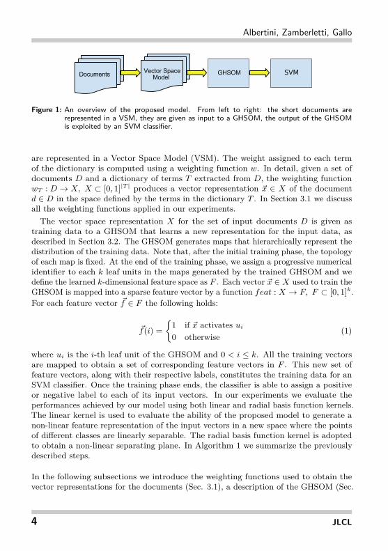
A detailed description of the proposed method is given in the following paragraphs. Thewhole training procedure is supervised: it consists of an unsupervised neural networkfor feature learning and a supervised classifier for document classification.In Figure 1 we present an overview of the proposed method: it is possible to
observe that the raw documents received as input by our feature learning algorithm
JLCL 2014 – Band 29 (1) 3
Albertini, Zamberletti, Gallo
SVM
Figure 1: An overview of the proposed model. From left to right: the short documents arerepresented in a VSM, they are given as input to a GHSOM, the output of the GHSOMis exploited by an SVM classifier.
are represented in a Vector Space Model (VSM). The weight assigned to each termof the dictionary is computed using a weighting function w. In detail, given a set ofdocuments D and a dictionary of terms T extracted from D, the weighting functionwT : D → X, X ⊂ [0, 1]|T | produces a vector representation ~x ∈ X of the documentd ∈ D in the space defined by the terms in the dictionary T . In Section 3.1 we discussall the weighting functions applied in our experiments.The vector space representation X for the set of input documents D is given as
training data to a GHSOM that learns a new representation for the input data, asdescribed in Section 3.2. The GHSOM generates maps that hierarchically represent thedistribution of the training data. Note that, after the initial training phase, the topologyof each map is fixed. At the end of the training phase, we assign a progressive numericalidentifier to each k leaf units in the maps generated by the trained GHSOM and wedefine the learned k-dimensional feature space as F . Each vector ~x ∈ X used to train theGHSOM is mapped into a sparse feature vector by a function feat : X → F, F ⊂ [0, 1]k.For each feature vector ~f ∈ F the following holds:
~f(i) ={
1 if ~x activates ui
0 otherwise(1)
where ui is the i-th leaf unit of the GHSOM and 0 < i ≤ k. All the training vectorsare mapped to obtain a set of corresponding feature vectors in F . This new set offeature vectors, along with their respective labels, constitutes the training data for anSVM classifier. Once the training phase ends, the classifier is able to assign a positiveor negative label to each of its input vectors. In our experiments we evaluate theperformances achieved by our model using both linear and radial basis function kernels.The linear kernel is used to evaluate the ability of the proposed model to generate anon-linear feature representation of the input vectors in a new space where the pointsof different classes are linearly separable. The radial basis function kernel is adoptedto obtain a non-linear separating plane. In Algorithm 1 we summarize the previouslydescribed steps.
In the following subsections we introduce the weighting functions used to obtain thevector representations for the documents (Sec. 3.1), a description of the GHSOM (Sec.
4 JLCL

Unsupervised feature learning for sentiment classification of short documents
Algorithm 1 Overview of the Proposed Model.Training
1. Build the dictionary of terms T from the set of all documents D.
2. Map all the training documents d ∈ D in the VSM representationwT (d) = ~x, ~x ∈ X using the dictionary T .
3. Train a GHSOM with the vectors in X. Once the training phase ends, the numberof maps generated by the GHSOM is k.
4. Each ~x ∈ X is mapped in the k-dimensional feature space F using the functionfeat(~x) = ~f . Let Y be the set of all the feature vectors computed in this way.
5. Train a SVM classifier using the feature vectors in Y along with their respectivelabels.
Prediction of a document d
1. Get the VSM representation ~x = wT (d).
2. Compute the corresponding feature vector ~f = feat(~x) using the trained GHSOM.
3. Predict the polarity of d by classifying the pattern f using the trained SVM.
3.2) and other shallow unsupervised feature learning algorithms used for comparison(Sec. 3.3).
3.1 Short Texts Representation
Here we describe how the short documents are represented in a VSM using a bag-of-words approach. Let D be the set of all documents and V be a vector space whosenumber of dimensions is equal to the number of terms extracted from the corpus. Usingan encoding function, we assign to each document d ∈ D a vector vd ∈ V , wherevd(i) ∈ [0, 1] is the weight assigned to the i-th term of the dictionary for the documentd. In our experiments we compare the results achieved by our model using five differentencoding functions that are presented in the following paragraphs.
Binary Term Frequency. It produces a simple and sparse representation of a shortdocument. Such representation lacks of representative power but acts as an informationbottleneck when provided as input to a classifier. It has also been adopted by Glorotet al. (2011b). Given a term t ∈ T and a document d ∈ D, Equation 2 is used tocompute the value of each weight.
JLCL 2014 – Band 29 (1) 5

Albertini, Zamberletti, Gallo
binary_score(d, t) ={
1 if t ∈ d0 otherwise
(2)
TF-IDF. It is a well-known method usually employed to compute the weights in aVSM. Using Equation 3, the weights assigned to a document d ∈ D is proportionalto the frequency of the term t in d (called tf) and it is inversely proportional to thefrequency of t in the corpus D (called df).
TF · IDF (d, t) = tf(d, t) · log( |D|df(D, t) ) (3)
In our experiments we compare the results obtained using the TF-IDF approach appliedboth to unigrams and unigrams plus bigrams.
Specific against Generic and One against All. In the following Equation wepresent a generic way to assign a weight to each term t in a document d:
score(t, sc, gc) = 1− 1log2(2 + Ft,sc·Dt,sc
Ft,gc)
(4)
sc and gc are two sets of documents representing the specific corpus and the genericcorpus respectively. We refer to the specific corpus as a set of documents that we wantto consider different from the ones in the generic corpus, as such this formula intendsto assign high scores to the terms of the documents in sc that are distinctive. Ft,sc
and Ft,gc are the frequencies of the term t in sc and gc respectively. The number ofdocuments in sc containing the term t is defined as Dt,sc.The weight assigned to each term t in d by Equation 4 is proportional to Ft,sc and
inversely proportional to Ft,gc; when t 6∈ gc, score(t, sc, gc) = 1 and when t 6∈ sc,score(t, sc, gc) = 0. Therefore, the value of the score function is proportional to theratio Ft,sc
Ft,gcand it is close to 0 when t is very frequent in gc (thus t is not a domain-specific
term).Using Equation 4, two weighting strategies are defined: (i) the Specific against
Generic (SaG), where sc is the set of positive-oriented documents and gc is the set ofnegative-oriented documents, (ii) the One against All (OaA), where sc is the set of allthe documents of our domain (both positive-oriented and negative-oriented documents)and gc is a set of documents that do not belong to the domain and semanticallyunrelated to the ones in sc.
3.2 GHSOM
In this section we describe the Growing Hierarchical Self-Organizing Map (GHSOM)model (Rauber et al., 2002).
6 JLCL
Unsupervised feature learning for sentiment classification of short documents
layer
1la
yer
2la
yer
3la
yer
0
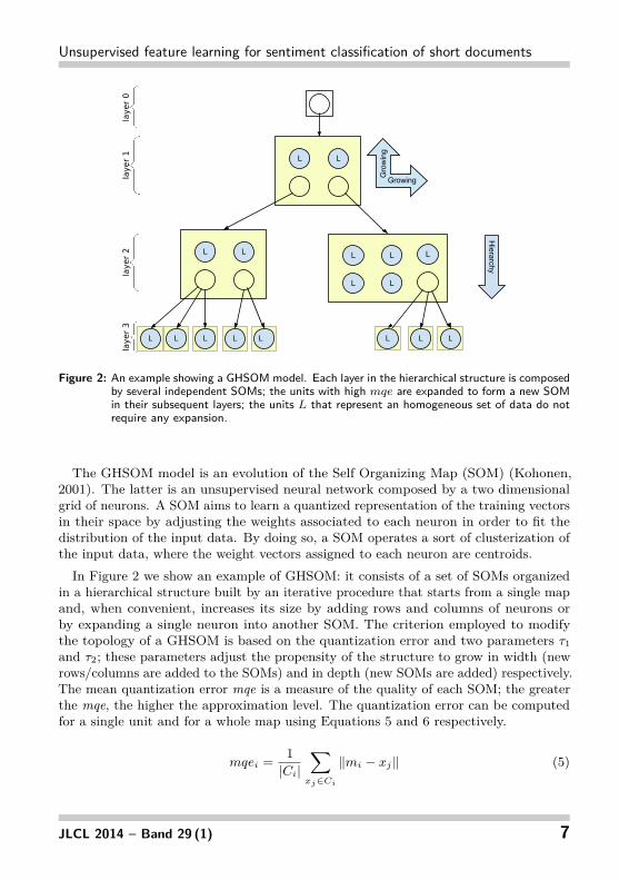
Figure 2: An example showing a GHSOM model. Each layer in the hierarchical structure is composedby several independent SOMs; the units with high mqe are expanded to form a new SOMin their subsequent layers; the units L that represent an homogeneous set of data do notrequire any expansion.
The GHSOM model is an evolution of the Self Organizing Map (SOM) (Kohonen,2001). The latter is an unsupervised neural network composed by a two dimensionalgrid of neurons. A SOM aims to learn a quantized representation of the training vectorsin their space by adjusting the weights associated to each neuron in order to fit thedistribution of the input data. By doing so, a SOM operates a sort of clusterization ofthe input data, where the weight vectors assigned to each neuron are centroids.In Figure 2 we show an example of GHSOM: it consists of a set of SOMs organized
in a hierarchical structure built by an iterative procedure that starts from a single mapand, when convenient, increases its size by adding rows and columns of neurons orby expanding a single neuron into another SOM. The criterion employed to modifythe topology of a GHSOM is based on the quantization error and two parameters τ1and τ2; these parameters adjust the propensity of the structure to grow in width (newrows/columns are added to the SOMs) and in depth (new SOMs are added) respectively.The mean quantization error mqe is a measure of the quality of each SOM; the greaterthe mqe, the higher the approximation level. The quantization error can be computedfor a single unit and for a whole map using Equations 5 and 6 respectively.
mqei = 1|Ci|
∑
xj∈Ci
‖mi − xj‖ (5)
JLCL 2014 – Band 29 (1) 7
Albertini, Zamberletti, Gallo
mqeM = 1|M |
∑
i∈M
mqei (6)
Let ui be the neuron of a SOM M , mi be the weight vector for ui and Ci be the setof the input vectors associated to ui.The training process begins with the creation of an initial map constituted by only
one unit whose weight vector is computed as the mean of all the training vectors. Thismap constitutes the layer 0 of the GHSOM and its mean quantization error is defined asmqe0. In the subsequent layer, a new SOMM1 is created and trained using the standardSOM training algorithm (Kohonen, 2001). After a fixed set of iterations, the meansquare error mqeM1 is computed and the unit ue having the maximum square error isidentified by computing e = argmaxi {mqei}. Depending both on the dissimilarity ofits neighbours and τ1, a new row or column of neurons is inserted at the coordinates ofthe unit ue. M1 is allowed to grow while the following condition holds:
mqeM1 ≥ (τ1 ·mqeM0 ) (7)
When Equation 7 is no longer satisfied, the units of M1 having high mqe may add anew SOM in the next layer of the GHSOM. The parameter τ2 is used to control whethera unit is expanded in a new SOM. A unit ui ∈M1 is subject to hierarchical expansionif mqei ≥ (τ2 ·mqe0).
The previously described procedure is recursively repeated to iteratively expand theSOMs both in depth and width. Note that each map in a layer is trained using onlythe training vectors clustered by its parent unit. The training process ends when nofurther expansions are allowed.
3.3 Other feature learning algorithms
The following algorithms can be used to learn a mapping for the input data from avector space to another and they are commonly used in literature to learn featuresfrom raw data in an unsupervised manner (Coates et al., 2011), as well as pre-traindeep architectures (Glorot et al., 2011b; Hinton and Salakhutdinov, 2006; Hinton et al.,2006).
3.3.1 Restricted Boltzmann Machine
A Restricted Boltzmann Machine (RBM) (Smolensky, 1986) is an undirected graphicalmodel composed by a visible layer and an hidden layer of neurons. The connectionsamong the units form a bipartite graph as each neuron of a layer is only connected tothe neurons in the other layer. The learned weights and biases can be used to obtain afeature mapping of the input vectors and this new representation may be provided to aclassifier.The training algorithm adopted in this work is the Contrastive Divergence (Hinton,
2002). This approximation of the gradient descent method has been employed usingmomentum and a L2 weight decay penalty. Both the neurons in the visible layer and
8 JLCL
Unsupervised feature learning for sentiment classification of short documents
the ones in the hidden layer use the logistic sigmoid activation function. We followedthe guidelines available in literature to easily implement and use a RBM (Hinton, 2010).
3.3.2 Autoencoder
Let X be the set of training vectors, an autoencoder is a neural network composedby an encoder function f(·) and a decoder function g(·) such that, given ~x ∈ X, thecomposition of the two functions gives the reconstructed input g(f(~x)) = r(~x). Thenetwork is trained to minimize the reconstruction error using the backpropagationalgorithm (Rumelhart et al., 1986). In this work we employ shallow autoencoderswith three layers (input, code and output). The code layer is used to generate a newrepresentation f(~x) for the input vectors that is provided as input to the classifier inthe same way a vector is generated using a RBM.
In our experiments, we evaluate three different activation functions for the neurons inthe code layer: logistic sigmoid, linear and rectified linear functions (Nair and Hinton,2010). The rectified linear function units are reported to work well on sentiment analysistasks (Glorot et al., 2011a). The momentum method has been used along with a L2weight decay penalty for regularization.
A variant consists in training the autoencoder to remove noise from the input vectors:gaussian noise with zero mean is added to the training set so that X +N(0, σ) = X;hence, the network is trained to reconstruct the data in X from X. In our experimentswe also use shallow denoising autoencoders with rectified linear units (Vincent et al.,2008).
4 Experiments
In this section we present the results obtained by performing an extensive experimentalanalysis of the proposed model. The main goal of our experiments is to determine: (i)how the parameters of our model affect its performances, (ii) the magnitude of thecontribution of the GHSOM and the SVM in the proposed model, (iii) how the GHSOMperforms in comparison with other state-of-the-art feature learning algorithms.
All our experiments are carried out using the Customer Review Dataset (Hu and Liu,2004). The dataset is composed by several annotated reviews associated to 5 differentproducts; each review consists of a set of short phrases whose lengths do not averagelyexceed 30 words. All the phrases are independently annotated, thus they can be treatedas short documents; moreover, their polarities can be predicted independently from thereviews they belong to. The Customer Review Dataset is composed by a total of 1095positive and 663 negative phrases; in our experiments we balance it so that the positiveand negative amounts of phrases are equal. This set of documents is splitted into atrain set and a test set: 70% of the positive and negative phrases forms the training setwhile the remaining data cases form the test set. This split is performed once and thenit is fixed and maintained during all the experiments.
JLCL 2014 – Band 29 (1) 9

Albertini, Zamberletti, Gallo
Table 1: F-measure values obtained by different stages of the proposed model for the CustomerReview Dataset. The columns labelled with SVM linear and SVM rbf show the baselineresults; the column labelled with GHSOM shows the results obtained by directly using aGHSOM as classifier; the last two columns show the sparse feature vector classification(SFVC) results obtained by the SVM with a linear and a radial basis function kernels.
Encoding SVMlinear
SVMrbf
GHSOM SFVC(linear)
SFVC(rbf)
Binary term frequency 0.52 0.56 0.75 0.81 0.87TF-IDF unigrams 0.55 0.57 0.76 0.76 0.86TF-IDF 2-grams 0.60 0.62 0.76 0.78 0.85Specific against generic 0.54 0.76 0.76 0.76 0.88One against all 0.56 0.56 0.77 0.81 0.90
All the meta-parameters both for the feature learning algorithms (such as τ1 and τ2for the GHSOM or the parameters for the algorithms in Sec. 3.3) and the SVM areselected using 5-fold cross-validation on the training set.
We evaluate the performances achieved by the proposed model using the F-measuredefined as in Equation 8.
F1 = 2 · p · r(p+ r) (8)
where p and r represent precision and recall values respectively.
Baseline. In the first part of our experiments, we measure the classification resultsusing the encodings described in Section 3.1; the vector representations generated bythose encodings are classified by an SVM with both linear or radial basis functionkernels, thus skipping the feature learning phase. As shown in Table 1, the resultsobtained using the linear and non-linear kernels are similar. That’s because the vectorspace has a great dimensionality, therefore mapping the data into an higher dimensionalnon-linear space does not improve the classification performances.
Note that this first part of the experiments is crucial for the subsequent phases: theunsupervised feature learning algorithm aims to learn a new space to generate newfeature vectors from those same input vectors. It is important to know whether theclassification of the data in the new space can outperform the results obtained just byusing a SVM with the same input vectors but without feature learning.
GHSOM analysis. In this second part of our experiments, we analyse the distributionof the documents in the clusters produced by a trained GHSOM.Given a trained GHSOM, we assign a polarity to each of its leaf units. Let ui be aleaf unit in the map M generated by an expansion of the unit upar belonging to theprevious layer. We define P = Ppos ∪ Pneg as the set of training vectors clustered bythe unit ui. The polarity assigned to ui is computed as follows:
10 JLCL
Unsupervised feature learning for sentiment classification of short documents
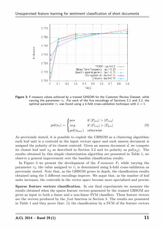
Figure 3: F-measure values achieved by a trained GHSOM for the Customer Review Dataset, whilevarying the parameter τ2. For each of the five encodings of Sections 3.1 and 3.2, theoptimal parameter τ1 was found using a k-fold cross-validation technique with k = 5.
pol(ui) =
pos if |Ppos| > |Pneg|neg if |Pneg| > |Ppos|pol(upar) otherwise
(9)
As previously stated, it is possible to exploit the GHSOM as a clustering algorithm:each leaf unit is a centroid in the input vectors space and each unseen document isassigned the polarity of its closest centroid. Given an unseen document d, we computeits closest leaf unit ud as described in Section 3.2 and its polarity as pol(ud). Theresults obtained by this simple clusterization algorithm are presented in Table 1; weobserve a general improvement over the baseline classification results.In Figure 3 we present the development of the F-measure F1 while varying the
parameter τ2; the value assigned to τ1 is determined using k-fold cross-validation aspreviously stated. Note that, as the GHSOM grows in depth, the classification resultsobtained using the 5 different encodings improve. We argue that, as the number of leafunits increases, the centroids in the vector space become more specialized and precise.
Sparse feature vectors classification. In our final experiments we measure theresults obtained when the sparse feature vectors generated by the trained GHSOM aregiven as input to both a linear and a non-linear SVM classifiers. These feature vectorsare the vectors produced by the feat function in Section 3. The results are presentedin Table 1 and they prove that: (i) the classification by a SVM of the feature vectors
JLCL 2014 – Band 29 (1) 11
Albertini, Zamberletti, Gallo
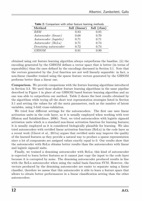
Table 2: Comparison with other feature learning methods.Method full (linear) full (rbm)RBM 0.83 0.85Autoencoder (linear) 0.68 0.70Autoencoder (logistic) 0.71 0.71Autoencoder (ReLu) 0.71 0.74Denoising autoencoder 0.72 0.74GHSOM 0.81 0.90
obtained using out feature learning algorithm always outperforms the baseline, (ii) theencoding generated by the GHSOM defines a vector space that is better (in terms ofseparability) than the ones defined by the encodings discussed in Section 3.1. Note thatthe vectors generated by the feat function are not well linearly separable: in fact, anon-linear classifier trained using the sparse feature vectors generated by the GHSOMperforms better than a linear one.
Comparison. We provide comparisons with the feature learning algorithms introducedin Section 3.3. We used those shallow feature learning algorithms in the same pipelinedescribed in Figure 1 in place of our GHSOM based feature learning algorithm and noone was able to outperform our method. Table 2 shows the best results obtained bythe algorithms while trying all the short text representation strategies listed in Section3.1 and setting the values for all the meta parameters, such as the number of latentvariables, using 5-fold cross-validation.
We tried four different settings for the autoencoders. The first one uses linearactivation units in the code layer, as it is usually employed when working with text(Hinton and Salakhutdinov, 2006). Next, we tried autoencoders with logistic sigmoidactivation units which is a standard non-linear activation function for learning features;it is usually employed as it is considered biologically plausible for learning. We alsotried autoencoders with rectified linear activation functions (ReLu) in the code layer asa recent work (Glorot et al., 2011a) argues that rectified units may improve the qualityof the learned features as they provide a natural way to produce a sparse representationsince a lot of components are assigned values exactly equal to 0. Our results show thatthe autoencoder with ReLu obtains better results than the autoencoders with linearand logistic sigmoid units.Finally, we trained a denoising autoencoder with ReLu; this kind of autoencoder
is expected to learn better features as it cannot just copy the input to the code layerbecause it is corrupted by noise. The denoising autoencoder produced results in linewith the ReLu autoencoder when using the radial basis function SVM. However, thevectors produced by the denoising autoencoder are easier to separate using a linearclassifier, therefore we assess that this autoencoder is able to learn a feature space thatallows to obtain better performances in a linear classification setting than the otherautoencoders.
12 JLCL
Unsupervised feature learning for sentiment classification of short documents
The RBM led to better results than the ones achieved by the autoencoders. Moreimportantly, the vector representation produced by the RBM led to better classificationresults than the ones obtained by our method when using a linear classifier; this meansthat the RBM learns a feature space that is better than the one of our GHSOM-basedalgorithm when the subsequent classification task is performed in a linear setting.However, as shown in Tables 1 and 2, it is not good enough to let the non-linearSVM overcome the best classification performance obtained by the proposed model,which learns a space that produces very effective feature vectors when classifying in anon-linear setting.
5 Conclusion
The method presented in this work is able to generate a sparse encoding of shortdocuments in an unsupervised manner, without using any prior knowledge related tothe context of the problem. In our experiments we proved that a properly trainedGrowing Hierarchical Self-Organizing Map, used as clustering algorithm for featurelearning and applied to different bag-of-word data representations, can provide robustresults. Excellent performances can be achieved when the output of such model isprovided as input to a Support Vector Machine classifier; thus, we argue the suitability offeature learning algorithms in the field of sentiment analysis. Our solution presents someinteresting advantages: (i) it is language independent, (ii) it does not require any lexiconof opinion-bearing words nor idioms, (iii) it is domain independent, meaning that it maybe applied to different contexts without further modifications. The comparison withother state-of-the-art unsupervised feature learning algorithms confirms the effectivenessof the proposed method: our feature learning model produces feature vectors that,once classified using a SVM classifier, lead to better performances compared to thestate-of-the-art algorithms that are similar to ours in characteristics and complexity.
References
Bengio, Y. (2009). Learning deep architectures for ai. Foundations and Trends in MachineLearning, 2(1):1–127.
Coates, A., Lee, H., and Ng, A. Y. (2011). An analysis of single-layer networks in unsupervisedfeature learning. In AISTATS.
Cortes, C. and Vapnik, V. (1995). Support-vector networks. Journal of Machine LearningResearch, 20(3):273–297.
Das, S. and Chen, M. (2001). Yahoo! for amazon: Extracting market sentiment from stockmessage boards. In In Asia Pacific Finance Association Annual Confference (APFA).
David M. Blei, A. Y. N. and Jordan, M. I. (2003). Latent dirichlet allocation. Journal ofMachine Learning Research, 3:993–1022.
JLCL 2014 – Band 29 (1) 13

Albertini, Zamberletti, Gallo
Ding, X., Liu, B., and Yu, P. S. (2008). A holistic lexicon-based appraoch to opinion mining.In Proceedings of First ACM International Conference on Web Search and Data Mining(WSDM).
Glorot, X., Bordes, A., and Bengio, Y. (2011a). Deep sparse rectifier neural networks. Journalof Machine Learning Research, 15:315–323.
Glorot, X., Bordes, A., and Bengio, Y. (2011b). Domain adaptation for large-scale sentimentclassification: A deep learning approach. In Proceedings of the 28th International Conferenceon Machine Learning (ICML).
Hatzivassiloglou, V. and McKeown, K. R. (1997). Predicting the semantic orientation ofadjectives. In Proceedings of the 35th Annual Meeting of the Association for ComputationalLinguistics (ACL).
Hinton, G. E. (2002). Training products of experts by minimizing contrastive divergence.Neural Computation, 14(8):1771–1800.
Hinton, G. E. (2010). A practical guide to training restricted boltzmann machines. Technicalreport.
Hinton, G. E., Osindero, S., and Teh, Y.-W. (2006). A fast learning algorithm for deep beliefnets. Neural Computation, 18(7):1527–1554.
Hinton, G. E. and Salakhutdinov, R. (2006). Reducing the dimensionality of data with neuralnetworks. Science, 313(5786):504–507.
Hu, M. and Liu, B. (2004). Mining and summarizing customer reviews. In Proceedings of the10th ACM SIGKDD International Conference on Knowledge Discovery and Data Mining(KDD).
Kanayama, H. and Nasukawa, T. (2006). Fully automatic lexicon expansion for domain-orientedsentiment analysis. In Proceedings of the Conference on Empirical Methods in NaturalLanguage Processing (EMNLP).
Kohonen, T. (2001). Self-Organizing Maps.
Ku, L.-W., Huang, T.-H., and Chen, H.-H. (2011). Predicting opinion dependency relations foropinion analysis. In Proceedings of 5th International Joint Conference on Natural LanguageProcessing (IJCNLP).
Maas, A. L., Daly, R. E., Pham, P. T., Huang, D., Ng, A. Y., and Potts, C. (2011). Learningword vectors for sentiment analysis. In Proceedings of the 49th Annual Meeting of theAssociation for Computational Linguistics (ACL).
Nair, V. and Hinton, G. E. (2010). Rectified linear units improve restricted boltzmann machines.In Proceedings of the 27th International Conference on Machine Learning (ICML), pages807–814.
Nakagawa, T., Inui, K., and Kurohashi, S. (2010). Dependency tree-based sentiment classifica-tion using crfs with hidden variables. In Human Language Technologies (HLT).
Pang, B. and Lee, L. (2008). Opinion mining and sentiment analysis. Foundations and Trendsin Information Retrieval, 2(1-2):1–135.
14 JLCL
Unsupervised feature learning for sentiment classification of short documents
Pang, B. and Vaithyanathan, S. (2002). Thumbs up? sentiment classification using machinelearning techniques. In Proceedings of the Conference on Empirical Methods in NaturalLanguage Processing (EMNLP).
Popescu, A. M. and Etzioni, O. (2005). Extracting product features and opinions from reviews.In Proceedings of the conference on Human Language Technology and Empirical Methods inNatural Language Processing (HLT/EMNLP).
Rauber, A., Merkl, D., and Dittenbach, M. (2002). The growing hierarchical self-organizingmap: Exploratory analysis of high-dimensional data. IEEE Transactions on Neural Networks,13:1331–1341.
Rumelhart, D. E., Hinton, G. E., and Williams, R. J. (1986). Learning representations byback-propagating errors. Nature, pages 533–536.
Smolensky, P. (1986). Parallel distributed processing: explorations in the microstructure ofcognition, vol. 1. chapter Information processing in dynamical systems: foundations ofharmony theory, pages 194–281. MIT Press.
Socher, R., Pennington, J., Huang, E. H., Ng, A. Y., and Manning, C. D. (2011). Semi-supervised recursive autoencoders for predicting sentiment distributions. In Proceedings ofthe Conference on Empirical Methods in Natural Language Processing (EMNLP).
Turney, P. D. and Littman, M. L. (2002). Unsupervised learning of semantic orientation froma hundred-billion-word corpus. Technical report, Technical Report EGB-1094, NationalResearch Council Canada.
Vincent, P., Larochelleand, H., Bengio, Y., and Manzagol, P.-A. (2008). Extracting and com-posing robust features with denoising autoencoders. In Proceedings of the 25th InternationalConference on Machine Learning (ICML).
Wen, M. and Wu, Y. (2011). Mining the sentiment expectation of nouns using bootstrappingmethod. In Proceedings of 5th International Joint Conference on Natural Language Processing(IJCNLP).
Wilson, T., Wiebe, J., and Hwa, R. (2004). Just how mad are you? finding strong and weakopinion clauses. In Proceedings of the 19th national conference on Artifical intelligence(AAAI).
Zhuang, L., Jing, F., and Zhu, X.-Y. (2006). Movie review mining and summarization. InProceedings of the 15th ACM international Conference on Information and KnowledgeManagement (CIKM).
JLCL 2014 – Band 29 (1) 15


Morgane Marchand, Romaric Besançon, Olivier Mesnard, Anne Vilnat
Domain Adaptation for Opinion Mining: A Study of Multi-polarity Words
Abstract
Expression of opinion depends on the domain. For instance, some words, called heremulti-polarity words, have different polarities across domain. Therefore, a classifiertrained on one domain and tested on another one will not perform well withoutadaptation. This article presents a study of the influence of these multi-polaritywords on domain adaptation for automatic opinion classification. We also suggest anexploratory method for detecting them without using any label in the target domain.We show as well how these multi-polarity words can improve opinion classification inan open-domain corpus.
1 Introduction
With the advent of the Social Web, the way people express their opinions has changed:they can now post product reviews on merchant sites and express their point of views onalmost anything in Internet forums, discussion groups, and blogs. Such online behaviourrepresents new and valuable sources of information with many practical applications.That is the reason why, in recent years, important research works have been undertakenon the subject of opinion mining. However, most works focus on how to characterizethe opinion of texts in a given corpus, which is often domain-specific (i.e. the opinionsin the texts are associated with the same type of objects), and little work have beendone on words with different polarity across domains. Some words can indeed changetheir polarity between two different domains (Navigli, 2012; Yoshida et al., 2011). Forexample, the word “return” has a positive connotation in the sentence “I can’t wait toreturn to my book”. However, it can be seen as very negative when talking about someelectronics device, as in “I had to return my phone to the store”. This phenomenonhappens even in more closely related domains: “I was laughing all the time” is a goodpoint for a comedy but a bad one for a horror film. We call such words or expressions“multi-polarity words”. This phenomenon is different from polysemy, as a word cankeep the same meaning across domains while changing its polarity which can lead toclassification error (Wilson et al., 2009). After a quick overview of the state of the art inthis field, we present our study on these multi-polarity words. In section 3, we show thata significant amount of multi-polarity words influences the results of common automaticopinion classifiers. Their deletion or their differentiation leads to better classificationresults. We are also interested in the automatic detection of multi-polarity words when
JLCL 2014 – Band 29 (1) – 17-31

Marchand, Besançon, Mesnard, Vilnat
there is no annotation in the target domain. We propose a solution to solve this issueby using a set of common pivot words in order to compare distribution of candidatemulti-polarity words in both domains. Finally, we show in section 4 that, even whena corpus does not contain explicit domain separation, the detection of multi-polaritywords in implicit domains improves the opinion classification.
2 State of the art
Subjective expressions are words and phrases being used to express mental andemotional states like speculation, evaluation, sentiment or belief (Wiebe et al., 2005;Wiebe and Mihalcea, 2006; Wilson, 2008; Akkaya et al., 2009). They are calledprivate states, that is to say, internal state which cannot be directly observed byothers (Quirk and Crystal, 1985). On the contrary, polarity refers to positive ornegative associations of a word or sense. Whereas there is a dependency in thatmost subjective senses have a relatively clear polarity, polarity can be attached toobjective words or senses as well. Su and Markert (2008) give the example of theword tuberculosis: it does not describe a private state, is objectively verifiable andwould not cause a sentence containing it to carry an opinion, but it does carry negativeassociations for the vast majority of people. Like Su and Markert (2008), we donot see polarity as a category that is dependent on prior subjectivity assignmentand therefore applicable to subjective sense only. There is of course some corre-lations. A subjective sense of a word is likely to appear in a polar expression butcan also appear in a neutral one. Similarly, an objective word can be used in a polar way.
Since a few years, interest on determining the polarity of ambiguous words hasgrown quickly (Wu and Jin, 2010). Practically all the existing annotation schemesfor polarity include a "both" or "varied" flag (Su and Markert, 2008; Wilson et al.,2005). In their classification of the causes of variation in contextual polarity, Wilsonet al. (2005) cite topic and domain. Moreover, in their study, Su and Markert (2008)notice that some preferences can exist depending on the domain or the topic of thetext. They report 32.5 % of subjectivity ambiguous words in their corpus and the wordsense disambiguation is not sufficient to remove the whole ambiguity. In Takamuraet al. (2006, 2007), the authors propose latent variable model and lexical network todetermine sentiment orientation of noun+adjective pairs. If the adjective is ambiguous,the classification is more difficult. Thus, the influence of domain on polarity is a veryimportant field of research. In this study, we are looking for words or expressions(subjective or objective as well) which carry polar associations in a specific domain.Many of the words we are looking at would have no inherent polarity but can occur inpolar contexts. We aim at imposing world knowledge and frequent discourse associationson these words.This work is related to contextual or target polarity (Wilson et al., 2005; Fahrniand Klenner, 2008). Fahrni and Klenner (2008) focus on the target-specific polaritydetermination of adjectives. A domain specific noun is often modified by a qualifying
18 JLCL

A Study of Multi-polarity Words
adjective. The authors argue that rather than having a prior polarity, adjectives areoften bearing a target specific polarity. In some case, a single adjective even switchespolarity depending on the accompanying noun. The authors use Wikipedia for auto-matic target detection and a bootstrapping approach to determine the target specificpolarity of adjectives. They achieve good results but focus only on adjectives. On thecontrary, Wilson et al. (2005) don’t restrict them on adjectives but work only withphrases containing pre-determined clues. They focus on phrase-level sentiment analysisand first determine whether an expression is neutral or polar before disambiguating thepolarity of the polar expression by using several rules and structural features.
In this study, we are interested in the influence of polarity-ambiguous words onpolarity at text level. In state of the art, most works deal with a pre-existent lexicon ofprior polarity. They aim at improving it, for example by weighting the different polarityof a word depending on the domain (Choi and Cardie, 2009). These particularizedlexicons can then be used by a rule-based classifier (Ding et al., 2008).As for studies on corpus-based only classifiers at text level, they focus mainly on therepresentation of data (Glorot et al., 2011; Huang and Yates, 2012). The adaptationerror of a classifier depends indeed on its performance on the source domain and onthe gap between source and target words distribution (Ben-David et al., 2007). Witha good projection, a link can be established between the words of the target domainwhich are missing from the source domain and the other words (Pan et al., 2010; Blitzeret al., 2007). However, if a word in a text has different polarity in source and targetdomain, it will still introduce an error. So, identification of multi-polarity words iscomplementary to these approaches and their improvements can be combined. However,the influence of words with several polarities on automatic classifiers is rarely studied.One noticeable exception is the work of Yoshida et al. (2011). They use a bayesianformulation and focus more precisely on the influence of the number of source andtarget domains, using up to fourteen domains.
In all these works, the object of study can vary. For example, Wilson et al. (2009)use a pre-existing lexicon of polar words. The coverage of their lexicon is 75 % of thepolar phrases of their corpus. On the contrary, Fahrni and Klenner (2008) focus onadjectives. In our study, we do not presume of what words or phrases are bearing polarinformation. We have chosen to automatically select them and classify them in onestep. Therefore, we have to be attentive to avoid selecting peculiarities of the corpus.As said before, we are working at text level. We are then interested on words or phraseswhich denote polarity at the text level. Some of them do not denote polarity at phraselevel and then would not be considered by previous work. Among these words andphrases, we are interested only on those we call multi-polarity words. That is to saythose which denote at text level a different polarity according to the general domain ofthe text.
JLCL 2014 – Band 29 (1) 19

Marchand, Besançon, Mesnard, Vilnat
3 A study of multi-polarity words
In this section, we present a study of multi-polarity words. The first part is dedicatedto a qualitative and quantitative study of these words. In a second part, we present anestimation of their influence on an usual automatic classifier. Finally, we explore thedetection of multi-polarity words without using any target label.
3.1 Description of the corpus
For this study, we have used the Multi-Domain Sentiment Dataset, collected by Blitzeret al. (2007). It contains four thematic corpora (DVDs, kitchen, electronics and books)of reviews collected on Amazon. Each corpus contains 1000 positive reviews, 1000negative reviews and some unlabelled reviews. These reviews are represented with abag of words of uni- and bi-grams. In this article, “word” is used to denote uni- orbi-grams.
3.2 Supervised detection of multi-polarity words
Multi-polarity words are first detected using a supervised approach, using the labelledreviews of each pair of thematic corpora. We make the common assumption thatpositive words will mostly appear in positive reviews and negative words in negativereviews. Then, for each word, we determine if its distribution in positive and negativereviews of target domain is statistically different or not from its distribution in positiveand negative reviews of source domain1. For that purpose, we use a χ2 test with a riskof false positive of 1%. The words are also selected only if they occur more often than agiven threshold (minOcc) and if their difference of positivity between the two domainsis higher than a second threshold (minDiff). These parameters are linked. If one ofthem is increased (less restrictive), the other one should be decreased (more restrictive)in order to keep the same level of performance. In a rank study, we have shown thatthey are approximatively linearly dependent.
Word region I loved worry compare returnelectronics 0.154 0.091 0.929 0.846 0.055
books 0.818 0.735 0.3 0.263 0.633
Table 1: Some example of percentage of presence in positive reviews for two domains. This scorerange from 0 (very negative) to 1 (very positive). A gap of 0.5 is then very significant (aneutral word becomes highly valued).
We present in Table 1 some multi-polarity words detected with this χ2 test. As wedetect our multi-polarity words based on a specific corpus, we have to be careful to
1Some words can have different polarity inside one domain but we only consider here the globalpolarity.
20 JLCL
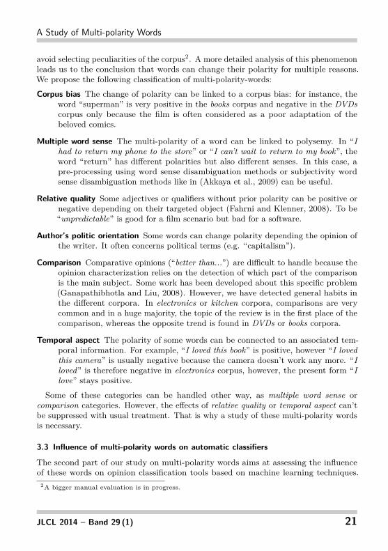
A Study of Multi-polarity Words
avoid selecting peculiarities of the corpus2. A more detailed analysis of this phenomenonleads us to the conclusion that words can change their polarity for multiple reasons.We propose the following classification of multi-polarity-words:Corpus bias The change of polarity can be linked to a corpus bias: for instance, the
word “superman” is very positive in the books corpus and negative in the DVDscorpus only because the film is often considered as a poor adaptation of thebeloved comics.
Multiple word sense The multi-polarity of a word can be linked to polysemy. In “Ihad to return my phone to the store” or “I can’t wait to return to my book”, theword “return” has different polarities but also different senses. In this case, apre-processing using word sense disambiguation methods or subjectivity wordsense disambiguation methods like in (Akkaya et al., 2009) can be useful.
Relative quality Some adjectives or qualifiers without prior polarity can be positive ornegative depending on their targeted object (Fahrni and Klenner, 2008). To be“unpredictable” is good for a film scenario but bad for a software.
Author’s politic orientation Some words can change polarity depending the opinion ofthe writer. It often concerns political terms (e.g. “capitalism”).
Comparison Comparative opinions (“better than...”) are difficult to handle because theopinion characterization relies on the detection of which part of the comparisonis the main subject. Some work has been developed about this specific problem(Ganapathibhotla and Liu, 2008). However, we have detected general habits inthe different corpora. In electronics or kitchen corpora, comparisons are verycommon and in a huge majority, the topic of the review is in the first place of thecomparison, whereas the opposite trend is found in DVDs or books corpora.
Temporal aspect The polarity of some words can be connected to an associated tem-poral information. For example, “I loved this book” is positive, however “I lovedthis camera” is usually negative because the camera doesn’t work any more. “Iloved” is therefore negative in electronics corpus, however, the present form “Ilove” stays positive.
Some of these categories can be handled other way, as multiple word sense orcomparison categories. However, the effects of relative quality or temporal aspect can’tbe suppressed with usual treatment. That is why a study of these multi-polarity wordsis necessary.
3.3 Influence of multi-polarity words on automatic classifiers
The second part of our study on multi-polarity words aims at assessing the influenceof these words on opinion classification tools based on machine learning techniques.
2A bigger manual evaluation is in progress.
JLCL 2014 – Band 29 (1) 21
Marchand, Besançon, Mesnard, Vilnat
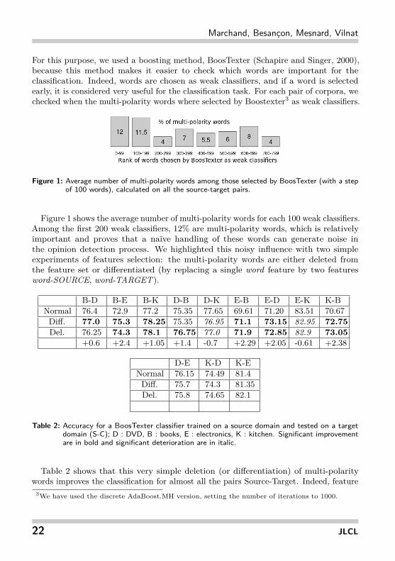
For this purpose, we used a boosting method, BoosTexter (Schapire and Singer, 2000),because this method makes it easier to check which words are important for theclassification. Indeed, words are chosen as weak classifiers, and if a word is selectedearly, it is considered very useful for the classification task. For each pair of corpora, wechecked when the multi-polarity words where selected by Boostexter3 as weak classifiers.
Figure 1: Average number of multi-polarity words among those selected by BoosTexter (with a stepof 100 words), calculated on all the source-target pairs.
Figure 1 shows the average number of multi-polarity words for each 100 weak classifiers.Among the first 200 weak classifiers, 12% are multi-polarity words, which is relativelyimportant and proves that a naïve handling of these words can generate noise inthe opinion detection process. We highlighted this noisy influence with two simpleexperiments of features selection: the multi-polarity words are either deleted fromthe feature set or differentiated (by replacing a single word feature by two featuresword-SOURCE, word-TARGET).
B-D B-E B-K D-B D-K E-B E-D E-K K-BNormal 76.4 72.9 77.2 75.35 77.65 69.61 71.20 83.51 70.67Diff. 77.0 75.3 78.25 75.35 76.95 71.1 73.15 82.95 72.75Del. 76.25 74.3 78.1 76.75 77.0 71.9 72.85 82.9 73.05
+0.6 +2.4 +1.05 +1.4 -0.7 +2.29 +2.05 -0.61 +2.38
D-E K-D K-ENormal 76.15 74.49 81.4Diff. 75.7 74.3 81.35Del. 75.8 74.65 82.1
Table 2: Accuracy for a BoosTexter classifier trained on a source domain and tested on a targetdomain (S-C); D : DVD, B : books, E : electronics, K : kitchen. Significant improvementare in bold and significant deterioration are in italic.
Table 2 shows that this very simple deletion (or differentiation) of multi-polaritywords improves the classification for almost all the pairs Source-Target. Indeed, feature
3We have used the discrete AdaBoost.MH version, setting the number of iterations to 1000.
22 JLCL

A Study of Multi-polarity Words
selection is known to be beneficial for domain adaptation (Satpal and Sarawagi, 2007).Moreover, a weighting of these multi-polarity words, rather than a complete deletion,is likely to give better results (Choi and Cardie, 2009). In a similar way, Akkayaet al. (2009) work on subjectivity ambiguous words and use subjectivity word sensedisambiguation in order to improve contextual classification of polarity at sentencelevel. They remove subjective words used in objective context and the accurracy oftheir automatic classifier improves of three points.These results justify the necessity of a dedicated handling of multi-polarity words, andof an automatic detection of these words in new domains.
3.4 Automatic detection of multi-polarity words in a new domain
The precedent study is based on a detection of multi-polarity words relying on anno-tations in both source and target domains. However, in a realistic application, theadaptation of a domain-specific opinion mining tool to a new domain has often to dealwith no or few annotations of target domain. Automatic labelling can be useful but isnot always possible. We present here our exploratory method for automatic detectionof multi-polarity words without any target annotation.
3.4.1 Overview of the approach
The proposed method relies on a list of pivot words. They should belong to bothsource and target domain, be useful for the opinion classification task and have a stablepolarity across domains. Their automatic selection is explained below. These pivotwords are used in order to compare the distribution of the others words in source andtarget domains. For each word, and for each domain, we create its co-occurrence profilewith respect to the list of pivot words. After that, a χ2 test is applied to decide if, for agiven word, its co-occurrence profiles in the source and target domains are statisticallydifferent (the word is considered as a multi-polarity word) or not (the word is then seenas a single-polarity word).
The pivot words are selected in two steps. First, a pre-selection is performed inorder to keep only words which appear nearly as many time in both domains and areat the same time useful for opinion classification in source domain. Then, an iterativeprocess removes from this list the words which have several polarities.For the pre-selection step, we first compute, using only the annotated documents fromthe source domain, the mutual information MIP,N between the presence or absence ofa word in a review and its positive/negative label. The selected pivot words shouldbe useful for opinion classification and therefore have a high value for this mutualinformation score. We set a minimum threshold on this MIP,N in order to keep at least1000 words. Following the same idea, we then compute, using the documents fromboth domains, the mutual information MIS,T between the presence and the absenceof a word in a review and its source/target label. Words which are not specific to adomain should then have a low value for this mutual information score. The pivot
JLCL 2014 – Band 29 (1) 23
Marchand, Besançon, Mesnard, Vilnat
words candidates are ranked using this MIS,T and only the 1000 words with the lowervalues of MIS,T are kept.After this pre-selection of pivot words, we detect the multi-polarity words among themusing the same procedure as described in previous section but on pivot words themselves.We remove from the list the word which is the most likely to change polarity. Then, weiterate the process until no more pivot words are detected as multi-polarity words.
3.4.2 Evaluation of the results
This automatic method selects too many words. Therefore, in an in-context evaluationlike in section 3.3, the accuracy drops drastically. In order to have an idea of thepertinence of our method, we have compared the words obtained automatically withour method (using only source labels) with those obtained by using labels of bothsource and target domains, as described in section 3.2. The automatic method selectsmore multi-polarity words (circa 1600 words) than the supervised one (circa 400 words),which explains the low precision score, as shown in table 3. Therefore, if all the detectedwords are deleted from the training corpus like in section 3.3, the accuracy is lower.However, precision can be increased without decreasing the recall by keeping only thewords which are detected as multi-polarity words with the higher confidence: the valuesare presented in the column max precision. This confirms that our method indeedselects the multi-polarity words first: more work must be undertaken to find the optimalthreshold for this selection.Moreover, if we only consider multi-polarity words which are actually used by theclassifiers (see figure 1), the average recall is 83.4 % for words selected in the first 100weak classifiers (column Recall 100 ) and 71.3 % for the first 300 weak classifiers (columnRecall 300 ). Therefore, the majority of multi-polarity words which are not detected arethose with few influence on opinion classification.So, despite a low precision, the results of our automatic detection method without usingany target annotation are very promising.
Precision tot. Recall tot. Precision max. Recall 100 Recall 30016 % 60.5 % 18.1 % 83.4 % 71.3 %
Table 3: Comparison between words selected by the automatic method with those selected by thesupervised one. The scores are the averaged recalls calculated on all the possible pairsSource-Target.
4 Use of multi-polarity words for open-domain opinion mining
In this section, we focus on another real case problem and present how to make use of themulti-polarity words in the context of opinion mining in open domain (i.e. in a generalcorpus that contains documents from different domains but without information on the
24 JLCL

A Study of Multi-polarity Words
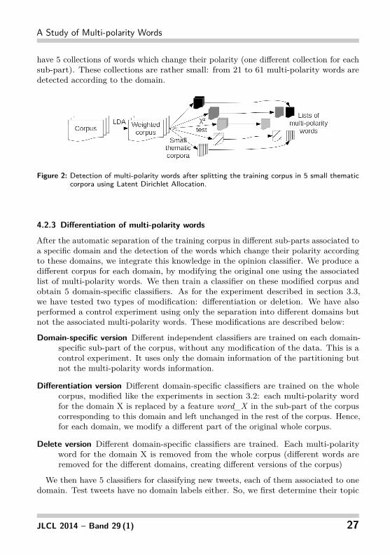
domains). In this context, we cannot rely on the domain labels to detect multi-polaritywords. We propose in this case to automatically find the different underlying domainsof the documents in order to separate the general training corpus into smaller thematiccorpora. Then, we apply the supervised detection method, presented in section 3.2, todetect multi-polarity words. These words are taken into account for learning severalspecific classifiers, one per thematic sub-corpus. The results of these classifiers aremerged to produce the final opinion classification.
4.1 Overview of the method
To make use of the multi-polarity words in a labelled open domain corpus, we firsthave to extract the underlying domains in the documents and assign each documentto a domain. We obtain several domains, not only two (one source and one target)like in the previous experiments. Therefore, we apply the supervised detection (3.2) ofmulti-polarity words several time, considering each domain versus all the others. Weobtain as many multi-polarity words lists as underlying detected domains. For eachmulti-polarity words list, we create a new training corpus by deleting or differentiatingthe words of the list like in section 3.3. Opinion classifiers are created on these newtraining corpora. At last, we have one classifier per underlying detected domain. Forclassifying a new text, we merge the answers of the different classifiers according to thedegree of relation of the new text to the underlying detected domains.
4.2 Evaluation
The evaluation of the proposed method is performed on the corpus of tweets from thetask 2 of SemEval 2013 (Wilson et al., 2013). These tweets are separated in threeclasses: positive, negative and neutral. We use as training corpus the training data,merged with the development data and we balance the different classes. So, our finalsystem is trained on 4500 tweets (1500 of each class, chosen randomly).First, we remove the web addresses from the tweets to reduce the noise. Then, weextract the emoticons and use the number of occurrences of each type (smile, tears,heart...) as features. Finally, we perform a lemmatization of the text, using the linguisticanalyser LIMA (Besançon et al., 2010). Table 4 shows a tweet example.
Bag of words features Emoticon type featurewow lady gaga be great Smile 1
Table 4: “WOW!!! Lady Gaga is great =)”
JLCL 2014 – Band 29 (1) 25

Marchand, Besançon, Mesnard, Vilnat
4.2.1 Domain generation
As the corpus has no domain label, we first have to identify the underlying domains andassign a domain to each tweet. For that purpose, we use Latent Dirichlet Allocation(LDA) (Blei et al., 2003). LDA has already been used in aspect-based review analysis,which is close to our work. In (Titov and McDonald, 2008a,b), the authors introduce amodel mixing global and local topics for aspect-based review analysis. They use themanual annotations of reviewers in order to improve the topics identification.In our experiment on tweets, we chose the Mallet LDA implementation (McCallum,2002).The framework uses Gibbs sampling to constitute the sample distributions whichare exploited for the creation of the topic model. The model is built using the lemmatizedtweets from the training and development data. We performed tests with differentnumbers of topics and the 5 topics version, presented in Table 5, appears to be themost efficient. Each tweet is then represented by a vector of length 5, where the i-thvalue is the proportion of words of the tweet which belong to the i-th topic.
Topic Film tonight, watch, time, todayTopic Obama win, vote, obama, blackTopic Sport game, play, win, team
Topic Informatic apple, international, sun, andersonTopic Show ticket, show, open, live
Table 5: Most representative words of each topic. We named the topics to make the presentationof data and results more readable.
Then, we subdivide the corpus in 5 sub-parts, or domain, each of them associatedwith one underlying detected topic. We have tested two types of subdivision. In thefirst one, called all training tweets version, a tweet is associated with its more relatedtopic. For example, if its proportion of words belonging to the topic sport is 55 %, thetweet will be part of the sub-part associated to sport domain. In the second subdivision,called domain confident training tweets version, a tweet is taken into account only ifmore than 75 % of its words belong to the same topic. Therefore, the precedent exampletweet will not be used. In this version, the sub-parts are more focused on only onetopic. In return, they contain less training tweets (2889 tweets altogether).
4.2.2 Detection of multi-polarity words
For detecting the multi-polarity words, we use the positive and negative labels of thetraining data, as described in the section 3.2. We apply this detection for each sub-part.Each time, we detect the words which change their polarity between a specific sub-partof the training corpus and its complement (all the others tweets). For example, theword “black” is detected as positive in the second sub-part, related to the election ofBarack Obama, and neutral in the rest of the tweets. At the end of this procedure, we
26 JLCL
A Study of Multi-polarity Words
have 5 collections of words which change their polarity (one different collection for eachsub-part). These collections are rather small: from 21 to 61 multi-polarity words aredetected according to the domain.
Figure 2: Detection of multi-polarity words after splitting the training corpus in 5 small thematiccorpora using Latent Dirichlet Allocation.
4.2.3 Differentiation of multi-polarity words
After the automatic separation of the training corpus in different sub-parts associated toa specific domain and the detection of the words which change their polarity accordingto these domains, we integrate this knowledge in the opinion classifier. We produce adifferent corpus for each domain, by modifying the original one using the associatedlist of multi-polarity words. We then train a classifier on these modified corpus andobtain 5 domain-specific classifiers. As for the experiment described in section 3.3,we have tested two types of modification: differentiation or deletion. We have alsoperformed a control experiment using only the separation into different domains butnot the associated multi-polarity words. These modifications are described below:
Domain-specific version Different independent classifiers are trained on each domain-specific sub-part of the corpus, without any modification of the data. This is acontrol experiment. It uses only the domain information of the partitioning butnot the multi-polarity words information.
Differentiation version Different domain-specific classifiers are trained on the wholecorpus, modified like the experiments in section 3.2: each multi-polarity wordfor the domain X is replaced by a feature word_X in the sub-part of the corpuscorresponding to this domain and left unchanged in the rest of the corpus. Hence,for each domain, we modify a different part of the original whole corpus.
Delete version Different domain-specific classifiers are trained. Each multi-polarityword for the domain X is removed from the whole corpus (different words areremoved for the different domains, creating different versions of the corpus)
We then have 5 classifiers for classifying new tweets, each of them associated to onedomain. Test tweets have no domain labels either. So, we first determine their topic
JLCL 2014 – Band 29 (1) 27

Marchand, Besançon, Mesnard, Vilnat
Figure 3: Flow of data. The modification is different for each version.
profile using LDA topic model. Then, we apply the 5 classifiers on the new tweet andobtain 5 answers. We use a mix of the 5 answers of the classifiers with weights accordingto the LDA mixture. This flow is presented in figure 3. We have tested several weightingschemes for this combination and the more efficient was the exponential of the LDAscore.
Figure 4: Average F-measure of positive and negative classes using two different training corpus:all training tweets or domain confident training tweets versions.
Figure 4 shows the results of these different integration of multi-polarity words usingthe two different initial training corpora created as described in section 4.2.1: all trainingtweets and domain confident training tweets versions.
28 JLCL
A Study of Multi-polarity Words
4.3 Analysis of the results and discussion
We have described a method to include domain information in an open-domain corpusto improve opinion classification at text level. As we do not have reference domain labelfor the documents, we create a partition using a detection of the latent topics using LDA.The Domain-specific version, which does not take into account the multi-polarity words,degrades the performances(-1.85% in the first experiment, -2.8% in the second). Wethink it is due to the rather small size of some training sub-corpora of the partition. Onthe contrary, the results with all the versions which integrate multi-polarity words showan improvement of the F-measure. We have tested the significance of this improvementwith a randomization test. In the case of the Delete version, the improvement issignificant (p-value is 0.03). The final improvement is rather small, however, it has tobe related to the small number of multi-polarity words we have detected (in average,36 words per domain). We think that the considered collection of tweets chosen for theevaluation is too small for the χ2 test to detect a lot of words with enough confidence.In comparison, in our experiment on reviews, we detected about 400 multi-polaritywords per domain. It is also worth noticing that for the domain confident experiment,the improvement is more sensible (+1.46% versus +0.70%) even if the absolute value ofthe score is not better, due to a much smaller training data. Moreover, in this case, thesignificance of the Delete version is higher (with a p-value of 0.005). These results arevery promising and show the interest of taking into account multi-polarity words.Another issue for this method is its dependency on the approach which is chosen toseparate the corpus into different domains. We used LDA for this purpose but we planto test a more supervised method using Explicit Semantic Analysis (Gabrilovich andMarkovitch, 2007) and based on the categories of Wikipedia, in order to have morecontrol on the domains (i.e. propose general domains that are not corpus-dependent).
5 Conclusion
In this article, we have studied the influence of multi-polarity words on the performanceof the automatic classification of opinion at text level. We have shown that these wordsare frequent and have influence on the performance of automatic classifiers in a corpusof domain-specific reviews and in an open-domain corpus of tweets. At the presenttime, a manual evaluation of these words is in progress. We discussed the real casewhere there is no labels available in the target domain and present an exploratorymethod for detecting multi-polarity words using carefully selected pivot words. Thenwe showed that the detection of multi-polarity words is also useful in an open-domaincorpus. Further works will be made on the selection criteria of multi-polarity words,especially in the case where no target label is used.
References
Akkaya, C., Wiebe, J., and Mihalcea, R. (2009). Subjectivity word sense disambiguation. InEMNLP.
JLCL 2014 – Band 29 (1) 29

Marchand, Besançon, Mesnard, Vilnat
Ben-David, S., Blitzer, J., Crammer, K., and Pereira, F. (2007). Analysis of representations fordomain adaptation. Advances in neural information processing systems, 19:137.
Besançon, R., el de Chalendar, G., Ferret, O., Gara, F., Mesnard, O., Laïb, M., and Semmar,N. (2010). Lima : A multilingual framework for linguistic analysis and linguistic resourcesdevelopment and evaluation. In Proceedings of LREC’10.
Blei, D. M., Ng, A. Y., and Jordan, M. I. (2003). Latent dirichlet allocation. the Journal ofmachine Learning research, 3:993–1022.
Blitzer, J., Dredze, M., and Pereira, F. (2007). Biographies, bollywood, boom-boxes andblenders: Domain adaptation for sentiment classification. In ACL.
Choi, Y. and Cardie, C. (2009). Adapting a polarity lexicon using integer linear programmingfor domain-specific sentiment classification. In EMNLP.
Ding, X., Liu, B., and Yu, P. S. (2008). A holistic lexicon-based approach to opinion mining.In Proceedings of WSDM, pages 231–240. ACM.
Fahrni, A. and Klenner, M. (2008). Old wine or warm beer: Target-specific sentiment analysis ofadjectives. In Symposion on Affective Language in Human and Machine, AISB Convention.
Gabrilovich, E. and Markovitch, S. (2007). Computing semantic relatedness using wikipedia-based explicit semantic analysis. In IJCAI, volume 7, pages 1606–1611.
Ganapathibhotla, M. and Liu, B. (2008). Mining opinions in comparative sentences. InProceedings of the 22nd International Conference on Computational Linguistics-Volume 1,pages 241–248. Association for Computational Linguistics.
Glorot, X., Bordes, A., and Bengio, Y. (2011). Domain adaptation for large-scale sentimentclassification: A deep learning approach. In ICML.
Huang, F. and Yates, A. (2012). Biased representation learning for domain adaptation. InEMNLP, pages 1313–1323, Jeju Island, Korea. Association for Computational Linguistics.
McCallum, A. K. (2002). Mallet: A machine learning for language toolkit.
Navigli, R. (2012). A quick tour of word sense disambiguation, induction and related approaches.SOFSEM 2012: Theory and Practice of Computer Science, pages 115–129.
Pan, S., Ni, X., Sun, J., Yang, Q., and Chen, Z. (2010). Cross-domain sentiment classificationvia spectral feature alignment. In WWW, pages 751–760. ACM.
Quirk, R. and Crystal, D. (1985). A comprehensive grammar of the English language, volume 6.Cambridge Univ Press.
Satpal, S. and Sarawagi, S. (2007). Domain adaptation of conditional probability models viafeature subsetting. In PKDD.
Schapire, R. and Singer, Y. (2000). Boostexter: A boosting-based system for text categorization.Machine learning, 39(2):135–168.
Su, F. and Markert, K. (2008). From words to senses: a case study of subjectivity recognition.In International Conference on Computational Linguistics.
30 JLCL
A Study of Multi-polarity Words
Takamura, H., Inui, T., and Okumura, M. (2006). Latent variable models for semanticorientations of phrases. In EACL.
Takamura, H., Inui, T., and Okumura, M. (2007). Extracting semantic orientations of phrasesfrom dictionary. In HLT-NAACL, pages 292–299.
Titov, I. and McDonald, R. (2008a). A joint model of text and aspect ratings for sentimentsummarization. In ACL.
Titov, I. and McDonald, R. (2008b). Modeling online reviews with multi-grain topic models.In WWW.
Wiebe, J. and Mihalcea, R. (2006). Word sense and subjectivity. In Proceedings of the 21stInternational Conference on Computational Linguistics and the 44th annual meeting of theAssociation for Computational Linguistics, pages 1065–1072. Association for ComputationalLinguistics.
Wiebe, J., Wilson, T., and Cardie, C. (2005). Annotating expressions of opinions and emotionsin language. Language resources and evaluation, 39(2-3):165–210.
Wilson, T., Kozareva, Z., Nakov, P., Ritter, A., Rosenthal, S., and Stoyanov, V. (2013).Semeval-2013 task 2: Sentiment analysis in twitter. In 7th International Workshop onSemantic Evaluation.
Wilson, T., Wiebe, J., and Hoffmann, P. (2005). Recognizing contextual polarity in phrase-levelsentiment analysis. In HLT/EMNLP.
Wilson, T., Wiebe, J., and Hoffmann, P. (2009). Recognizing contextual polarity: An explorationof features for phrase-level sentiment analysis. Computational Linguistics, 35:339–433.
Wilson, T. A. (2008). Fine-grained subjectivity and sentiment analysis: recognizing the intensity,polarity, and attitudes of private states. ProQuest.
Wu, Y. and Jin, P. (2010). Semeval-2010 task 18: Disambiguating sentiment ambiguousadjectives. In 5th International Workshop on Semantic Evaluation, pages 81–85.
Yoshida, Y., Hirao, T., Iwata, T., Nagata, M., and Matsumoto, Y. (2011). Transfer learningfor multiple-domain sentiment analysis - identifying domain dependent/independent wordpolaritys. In AAAI.
JLCL 2014 – Band 29 (1) 31


Josef Ruppenhofer, Julia Maria Struß, Jonathan Sonntag, Stefan Gindl
IGGSA-STEPS: Shared Task on Source and Target Extractionfrom Political Speeches
Accurate opinion mining requires the exact identification of the sourceand target of an opinion. To evaluate diverse tools, the research communityrelies on the existence of a gold standard corpus covering this need. Sincesuch a corpus is currently not available for German, the Interest Group onGerman Sentiment Analysis decided to create such a resource and makeit available to the research community in the context of a shared task. Inthis paper, we describe the selection of textual sources, development ofannotation guidelines, and first evaluation results in the creation of a goldstandard corpus for the German language.
1 Introduction
Opinion source and target extraction is the area of opinion mining aiming at identifyingthe source (i.e., whose opinion?) as well as the target (i.e., about what?) of an opinion.It is applicable to free language texts, where this kind of information cannot be derivedfrom meta-data. Source and target extraction turns out to be a surprisingly difficulttask. Intuitively, humans should be easily capable of accomplishing it, yet they oftenfounder on the subtleties of language. While a brief glance at a text gives the impressionof an easily solvable task, delving into it reveals its complexity. A varying numberof sources/targets might confuse the reader, in other cases the source/target mightnot be present in the sentence, or it is difficult to decide on the linguistic span of thesource/target. A task so difficult to solve for humans poses an even bigger challenge forcomputers. With their at most limited understanding of human language, solving sucha task requires sophisticated algorithms. This is aggravated by the fact that the datapublicly available for machine learning purposes is too sparse.The paper we present here summarizes the efforts of the Interest Group of German
Sentiment Analysis (IGGSA)1 to create a publicly available resource serving as a goldstandard corpus for opinion source and target extraction. The corpus consists of alarge number of speech transcripts from debates in the Swiss parliament and containsannotations for the evaluation of source and target extraction systems. IGGSA plansto use the corpus as part of a shared task focusing on source and target extractionfrom political speeches (STEPS) in the run-up to the KONVENS conference 2014 inHildesheim.
1https://sites.google.com/site/iggsahome/
JLCL 2014 – Band 29 (1) – 33-46

Ruppenhofer, Struß, Sonntag, Gindl
In this paper we discuss the choice of Swiss parliament speeches, report the detailsof the annotation guidelines and show evaluation results of a first round of manualannotations.
2 Related Work
An important aspect of opinion mining systems is their ability to establish a connectionbetween subjective expressions and their sources and targets. A system capable of doingthis provides a holistic picture of an expressed opinion. Sentiment analysis systems mustbe able to reliably tie opinions or subjective states to their sources and targets. This isa non-trivial task as some sentiment-bearing expressions are not linked to the sources,and some not even to the targets, of opinion. In the best case, the source and targetcorrespond to semantic roles of sentiment-bearing predicates that can be expressed assyntactic arguments (Ruppenhofer et al., 2008). For instance, the subject of love in(1) is the source of the positive sentiment expressed and the object is the target of thesentiment.(1) I really love the players and the staff. [www]
However, a direct tie-in with semantic role labeling is usually not the chosen way ofhandling the extraction of sources and targets. In the following, we discuss the reasonsfor this and some of the alternative problem statements that have been adopted.
2.1 Attribution and nesting of sources
In the case of one important sub-class of sentiment-bearing expressions, called expressivesubjective elements by Wiebe et al. (2005), a grammatical link exists between the opinionexpression and the target2, but not necessarily to the source. For instance, in the caseof idiotic we know that what the adjective modifies or is predicated of is the target ofthe sentiment conveyed. Thus, “exit” is the target in (2) and “[t]hat” is the target in(3). Note, however, that the sources differ between the two examples: in (2), the sourceis the writer of the text, whereas in (3) it is the quoted speaker Irvine.(2) His rude, crude response and idiotic exit from his duties is hardly deserving
of the praise he has attracted. [www]
(3) “That was idiotic,” Irvine told talkSPORT . [www]Rather than connect expressions of opinion only to their immediate sources, it is
desirable to keep track of the chain of transmission. In the MPQA-corpus (Wiebe et al.,2005), for instance, levels of nesting are recorded that would show for a sentence like (3)that not only is Irvine the source of the opinion expressed by idiotic but that we cometo know this only via an utterance of the writer of the text in which Irvine’s speech ispresented. In the annotations we produce, nesting is not explicitly marked but can bereconstructed from the annotations, as discussed in Section 3.3.
2This link may either take the form of a predicate-argument or a modifier-head relationship.
34 JLCL

IGGSA-STEPS
2.2 Definitions of target
The main issue with respect to targets is whether the analysis should address only whatone may call “local” targets, that is expressions that are semantic valents and syntacticdependents of a particular sentiment-bearing predicate, or whether it should also takeinto account other targets that are pragmatically relevant. To illustrate the difference,consider the following pair of examples:
(4) a. I am not a Dortmund fan – I am a Schalke fan – but I am glad+[Dortmund beat Bayern]Target.
b. I am not a Dortmund fan – I am a Schalke fan – but I am glad Dortmundbeat- [Bayern]Target.
Example (4a) displays the stable, “literal” sentiment that is conveyed by the sentence:that the speaker is glad about the reported event. Example (4b), by contrast, displaysan inferred sentiment: that the speaker specifically dislikes Bayern’s team. The inferredsentiment toward Bayern may be canceled if the context was further elaborated, forinstance by emphasizing a merely financial interest in the outcome (“If they hadn’t, Iwould have lost my 100 e bet on that game”).
Stoyanov and Cardie (2008) adopt a very pragmatic understanding of targets. Theysuggest a definition of opinion topic and present an algorithm for opinion topic identifi-cation that casts the task as a problem in topic co-reference resolution. In their work,they distinguish between:
“Topic The Topic of a fine-grained opinion is the real-world object, event or abstractentity that is the subject of the opinion as intended by the opinion source.
Topic span The Topic Span associated with an Opinion Expression is the closest,minimal span of text that mentions the topic.
Target span In contrast, Target Span denotes the span of text that covers the syntacticsurface form comprising the contents of the opinion.” (Stoyanov and Cardie, 2008,p. 818)
Notice the absence of any reference to syntactic relations between the subjectiveexpression and the topic span, and the emphasis on the intentions of the opinion sourcefor the identification of the topic. Given their definitions, Stoyanov and Cardie (2008)analyze the following example as indicated by the brackets and markup.
(5) [OH Al] thinks that [TARGET SPAN [TOPIC SPAN? the government] should[TOPIC SPAN? tax gas] more in order to [TOPIC SPAN? curb [TOPIC SPAN?CO2 emissions]]]. (= ex. (2), Stoyanov and Cardie, 2008, p. 818)
In example (5), the target span consists of the complement of think and there aremultiple potential topics (denoted by the question marks in example 5) within thesingle target span of the opinion, each of them identified with its own topic span. This
JLCL 2014 – Band 29 (1) 35

Ruppenhofer, Struß, Sonntag, Gindl
illustrates that, at the text level, certain inferred targets might be more important thanthe overt target. In our annotations, targets correspond mostly to Stoyanov and Cardie(2008)’s target spans. What they consider as alternative topic spans relative to thesame subjective expression is captured as targets of inferred opinions in our schemeand annotated in addition to the basic opinion that has their ’target span’ as its target.
2.3 Prior Shared Tasks
While quite a few shared tasks have addressed the recognition of subjective unitsof language and, possibly, the classification of their polarity (SemEval 2013 Task 2,Twitter Sentiment Analysis (Nakov et al., 2013); SemEval-2010 task 18: Disambiguatingsentiment ambiguous adjectives (Wu and Jin, 2010); SemEval-2007 Task 14: AffectiveText (Strapparava and Mihalcea, 2007) inter alia), few tasks have included the extractionof sources and targets.The most relevant prior work was done in the context of the Japanese NTCIR3
Project. In the NTCIR-6 Opinion Analysis Pilot Task (Seki et al., 2007), which wasoffered for Chinese, Japanese and English, sources and targets had to be found relative towhole opinionated sentences rather than individual subjective expressions. However, thetask allowed for multiple opinion sources to be recorded for a given sentence if multipleopinions were expressed. The opinion source for a sentence could occur anywhere inthe document. In the evaluation, where necessary, co-reference information was used to(manually) check whether a system response was part of the correct referent’s chainof mentions. The sentences in the document were judged as either relevant (Y) ornon-relevant (N) to the topic (=target). Polarity was determined for each opinionatedsentence, and for sentences with more than one opinion expressed, the polarity of themain opinion expressed was chosen. All sentences were annotated by three assessors,allowing for strict and lenient (by majority vote) evaluation. The successor task, NTCIR-7: Multilingual Opinion Analysis (Seki et al., 2008), was basically similar in its setup toNTCIR-6, but also considered annotations relative to sub-sentences or clauses.While the STEPS-task will focus on German, the most important difference to the
shared tasks organized by NTCIR, as we will illustrate below, is that it defines the sourceand target extraction task at the level of individual subjective expressions. There is noshared task annotating at the expression level, rendering existing guidelines impracticaland making the development of guidelines from scratch necessary. The corpus will beavailable for further annotation by ourselves and other research groups.
2.4 Corpora of political language
The usage of political corpora for NLP tasks is well-established within the scientificcommunity. Thomas et al. (2006) collected US Congressional Speech Data, containingsegments of uninterrupted speech. Guerini et al. (2008) constructed a corpus of taggedpolitical speeches (CORPS), containing 3600 English-language speeches harvested from
3NII [National Institute of Informatics] Test Collection for IR Systems
36 JLCL

IGGSA-STEPS
the web. The authors focused on audience reactions and tagged applause or laughter tomake these response signals usable as identifying markers of persuasive communications.Osenova and Simov (2012) built a corpus of Bulgarian political speeches containingboth interviews with politicians as well as debates from the years 2006 to 2012. Ithas annotations for topic, turns, and linguistic units. Analysis of sentiment/opinionsis in progress. Closer to our concerns in terms of the data used, Barbaresi (2012)constructed a corpus containing the political speeches by German presidents andchancellors (Bundespräsidentenkorpus: 1442 speeches (1984-2012); Bundeskanzlerkorpus:1831 speeches (1998-2011)).
In a previous effort to create a gold-standard corpus for German opinion mining,IGGSA created MLSA, the Multi-Layered Sentiment Analysis corpus (Clematide et al.,2012). This corpus, consisting of 270 sentences crawled from news websites, is annotatedat three levels: (i) the sentence-level, covering subjectivity and overall polarity of asentence, (ii) word- and phrase-level, and (iii) expression-level, focusing on objectiveand direct speech events. While the expression-level annotation of the MLSA is similarin spirit to the annotations created here, the corpus as such is ultimately not suitablefor our purposes because the sentences in the MLSA do not form full texts. They weresampled out of the larger Sdewac-Corpus (Faaß and Eckart (2013)), which containsparsable sentences from the web in scrambled order.
2.5 Summary
In summary, our annotation scheme picks up most of the linguistic features that havebeen pursued in related work. It is, however, ultimately distinct from prior work.For instance, we choose a simpler treatment in some cases such as targets where wefollow grammar more closely and concentrate on arguments, whereas Stoyanov andCardie (2008) are interested in topic spans with text-level relevance. In other cases,our treatment is implicit, as in the case of the nesting of sources, which, unlike Wiebeet al. (2005), we do not annotate explicitly. And, finally, unlike all prior shared tasks,we annotate at the expression level.
3 Definition of the STEPS-Shared Task
Given the difficulty of the tasks as well as the diversity of systems that researchers areworking on, the STEPS shared task will offer one main task as well as two subtasks:
Main task Identification of subjective expressions with their respective sources andtargets
1st subtask Participants are given the subjective expressions and are only asked toidentify opinion sources.
2nd subtask Participants are given the subjective expressions and are only asked toidentify opinion targets.
JLCL 2014 – Band 29 (1) 37
Ruppenhofer, Struß, Sonntag, Gindl
We allow for participation in any combination of the tasks. However, so as to notgive an unfair advantage to any participants, the main task is run and evaluated firstbefore the gold information on subjective expressions is given out for the two subtasks,which will be run concurrently.
3.1 Data
The STEPS data set comes from the Swiss parliament (Schweizer Bundesversammlung).The choice of this particular data set is motivated as follows: (i) the source data is opento the public and allows for free distribution with the annotations4; (ii) the text allowsfor annotation of multiple sources and targets; (iii) the text meets the research interestsof several IGGSA-members, i.e. supports collaborations with political scientists andresearchers in digital humanities.Since the Swiss parliament operates multi-lingually, we decided to discard not only
non-German speeches but also German speeches that respond to, or comment on,speeches, heckling, and side questions in languages other than German. This was doneso that no German data had to be annotated whose correct interpretation might dependon foreign-language material that our annotators might not be able to understand fully.Additional potential difficulties derive from peculiarities of Swiss German found in
the data. For instance, the vocabulary of Swiss German is different from standardGerman, often in subtle ways. For instance, the verb vorprellen is used in 6 instead ofvorpreschen, which would be expected for German spoken in Germany.
(6) Es ist unglaublich: Weil die Aussenministerin vorgeprellt ist , kann man dasnicht mehr zurücknehmen .’It is incredible: because the foreign secretary acted rashly, we can’t take thatback again.’
In order to minimize any negative impact that might result from the misunderstan-ding of Swiss German by our German and Austrian annotators, we chose speechesrelated to what we considered non-parochial topics. For instance, we used texts relatedto international affairs rather than to Swiss municipal governance. In addition, theannotation guidelines encourage annotators to mark annotations as Swiss Germanwhen they involve language usage that they are not fully familiar with. Such cases canthen be excluded or weighed differently for the purposes of system evaluation. In ourannotation, such markings are in fact rare. We think this reflects the fact that althoughparliamentary speeches are medially spoken, they are conceptually written, and we findmuch less Swiss German vocabulary than one would expect in Swiss German colloquialspeech (cf. Scherrer and Rambow (2010)).
The STEPS data set has the following pre-processing pipeline: sentence segmentationand tokenization using OpenNLP5, lemmatization with the TreeTagger (Schmid, 1994),constituency parsing using the Berkeley parser (Petrov and Klein, 2007), and conversion
4We were not able to conclusively ascertain the copy rights for German parliamentary speeches.5http://opennlp.apache.org/
38 JLCL

IGGSA-STEPS
Exact Match Partial MatchSubjective Expression 0.7634 0.8314Sources (when SE match) 0.5685 0.5959Targets (when SE match) 0.4521 0.7123
Table 1: Inter-annotator agreement for the second annotation step
of the parse trees into TigerXML-Format using TIGER-tools (Lezius, 2002). For theannotation we used the Salto-Tool (Burchardt et al., 2006).
3.2 Development of the annotation scheme
The different research interests of the IGGSA-members called for a novel annotationscheme, which we based on a first explorative annotation step. In this step, fourannotators labeled a mutual set of 50 sentences with respect to opinions, targets andsources. The sole requirement was the annotation of sources and targets at the level ofindividual subjective expressions and consideration of all nested targets and holders.The annotators reported on annotation decisions to support the development of a firstannotation scheme and formed an initial set of guidelines.
In a second step, two experienced annotators re-annotated the data using the initialguidelines and assessed them. The average inter-annotator agreement, i.e. the recall ofannotations from both annotator perspectives, also took partial matches into conside-ration as proposed in Wiebe et al. (2005). Table 1 shows the results; we observed anagreement of 83% for subjective expressions (Wiebe et al. (2005) reports an averageagreement of 72%) and 71% on targets. Cases of disagreement were subject to furtheranalysis to enhance the guidelines.
3.3 Guidelines used
Generally, our annotation scheme can be characterized as a single-stage scheme aimingat full coverage.6 That is, we only annotate at the expression level – we do not performsentence or document-level annotations prior or subsequent to the expression-levelannotation. And any and all kinds of subjective expressions by any source and on anytopic were to be annotated. There was thus no focus on particular politicians, parties,issues etc. as potential sources or targets.
Our definition of subjective expressions is broad and based on well-known prototypes.It covers expressions of
• evaluation (positive or negative): toll ’great’, doof ’stupid’
• (un)certainty: zweifeln ’doubt’, gewiss ’certain’
• emphasis: sicherlich/bestimmt ’certainly’6See https://sites.google.com/site/iggsahome/downloads for the final form of the guidelines.
JLCL 2014 – Band 29 (1) 39

Ruppenhofer, Struß, Sonntag, Gindl
• speech acts: sagen ’say’, ankündigen ’announce’
• mental processes: denken ’think’, glauben ’believe’
Our list of prototypes is inspired by, and largely overlaps with, the notions thatWiebe et al. (2005) subsumes under the umbrella term private state, following Quirket al. (1985): “As a result, the annotation scheme is centered on the notion of privatestate, a general term that covers opinions, beliefs, thoughts, feelings, emotions, goals,evaluations, and judgments.” However, beyond giving the prototypes, we did not seekto impose any particular theory from the linguistic or psychological literature relatedto subjectivity, appraisal, emotion or related notions.We initially intended to distinguish polar facts from proper opinions. As we had
conceived of the difference, polar facts were expressions whose status as subjectivedepended on context and for which even differences in polarity depending on context areconceivable (cf. 7a versus 7b), whereas real opinions result from the inherent meaningof words and syntactic patterns.
(7) The car interior uses a lot of plastic. (constructed)a. That’s great because it saves weight and, thus, gas.b. It looks very cheap and inelegant.
However, we abandoned this plan after observing low agreement in intermediate roundsof annotation. In our final annotation round, polar facts could optionally be distinguishedby setting a flag marking them as ’inferred’ opinions on a subjective expression frame.
Further, no type of lexical or multi-word expression, or syntactic pattern was excludedfrom consideration. Thus, depending on the actual use in context, annotators could, forinstance, mark as subjective expressions:
• exclamation marks
• rhetorical devices (marked also by a flag of the same name), chief among them:– repetitions (Ein Beschluss für Klimaschutz ist an Deutschland geschei-tert, an deutschen Abgeordneten, an Konservativen und Libera-len, . . .. ’A proposal for climate protection failed because of Germany,because of German MPs, because of conservatives and liberals, . . .’ 7)
– emphatically spelled words– rhetorical questions (Und wer soll das bezahlen? ’And who is supposed
to pay for that?’)
In identifying subjective expressions, annotators were instructed to select minimalspans where possible. This instruction went hand in hand with the decision that for thepurposes of the shared task we would set aside any treatment of polarity and intensity.
7http://dip21.bundestag.de/dip21/btp/17/17240.pdf
40 JLCL

IGGSA-STEPS
Thus, negation, intensifiers and attenuators and any other expressions that might affecta minimal expression’s polarity or intensity could be ignored.An important aspect of the scheme is that the same expression could be labeled
multiple times as a subjective expression with its own source and target. The need forthis multi-layer annotation arises, for instance, in cases where a lexical item evokes twoevaluations (cf. Maks and Vossen (2011)). The verb prahlen ’brag’, for instance, conveysa positive evaluation by a participant in the event about another participant, and asecond negative evaluation about an event participant by the speaker who uses the wordprahlen. The need for multiple annotations also arises when multiple different semanticroles are evaluated. For instance, with verbs like danken ’thank’ or beschuldigen ’accuse’,arguably both a person and their behavior can be seen as targets of evaluation.With respect to sources and targets, annotators were instructed to first consider
syntactic/semantic dependents of the subjective expressions. If sources and targets werelocally unexpressed, they could look further in the context and annotate other phrases.8In cases where a subjective expression represented the view of the implicit speaker/textauthor, annotators could set a flag ’Speaker’ (Sprecher) on the source element. Notethat the nesting of sources is not explicitly captured by our scheme. However, implicitly,it is captured as follows: a subjective expression A that is embedded within the targetof another subjective expression B should have a source that is embedded under thesource of expression B (see example (4) in Section 2.2).
4 Inter-annotator agreement
After the revision of the annotation guidelines as described above, five unseen speechesof the Swiss parliament, consisting of approximately 200 sentences, were selected for aproof-of-concept annotation round. Two groups, each consisting of three annotators,annotated about 100 sentences (two or three documents respectively). Both groupsconsisted of one experienced annotator and two master-level students, the latter havingbeen trained for the annotations by a presentation of the annotation guidelines andexample annotations. The inter-annotator agreement can be found in Tables 2 and 3.The first one shows the average pairwise inter-annotator agreement and the second onethe agreement for the full-agreement mode, containing only those cases, where therewas at least a partial match on the subjective expression level for all three annotators.All shown values include exact and partial matches. In addition, we always give theaverage dice coefficient (see equation 8), which we used for measuring the similarity ofthe annotations with respect to the overlapping terminals.
dice = 2 ∗ matching terminalsterminals annotated by A1 + terminals annotated by A2 (8)
8For the actual shared task, we plan on adding a layer of co-reference annotations to the data sothat systems do not need to match a particular mention of the relevant source or target to receivecredit.
JLCL 2014 – Band 29 (1) 41

Ruppenhofer, Struß, Sonntag, Gindl
group 1 group 2Armut1 Aussen1 Aussen2 Buchpreis1 Buchpreis2 mean3
Sources1.2 0.5375 0.4453 0.6742 0.7585 0.6605 0.6186Dice acrosssource mat-ches
1.0000 0.9871 0.9977 0.9831 0.9896 0.9887
Targets1.2 0.6849 0.5384 0.5938 0.7883 0.6598 0.6549Dice acrosstarget mat-ches
0.7017 0.7058 0.7154 0.8406 0.8322 0.7722
SubjectiveExpression1
0.5728 0.4629 0.6456 0.5774 0.6554 0.5671
Dice acrossSubjectiveExpressionmatches1
0.8361 0.6538 0.5865 0.8901 0.7951 0.7563
1including exact and partial matches2only considering cases with a match on the level of the subjective expression3weighted by no. of sentences in the speeches
Table 2: Average pairwise inter-annotator agreement with a total number of annotated subjectiveexpressions per annotator between 145 and 262 for group 1 and 122 and 236 for group 2
When comparing the agreement of the second annotation iteration (Table 1) and theproof-of-concept annotations (Table 2), a decrease in agreement of about 25%-pointscan be seen on the level of subjective expressions and a smaller decrease of about6%-points to about 65.5% on the level of targets, but also a small increase of about2%-points to 62% regarding source annotations. Considering that the annotators in thelatter round were mostly unexperienced in this kind of task, and also considering thatthere were more annotators, leaving room for more disagreement, the results for thesource and target annotations are quite satisfying, especially given the complexity ofthe annotation task. Compared to inter-annotator agreement studies of the previouslymentioned NTCIR (M)OAT tasks, who reported an average pairwise agreement onopinionated judgements between κ = 0.23 (Chinese) and 0.67 (Japanese) in the first year(cf. Seki et al., 2007, p. 269) and 0.23 (English) and 0.71 (Japanese) in the second year(cf. Seki et al., 2008, p. 190, 193) and 0.46 (trad. Chinese) and 0.97 (simpl. Chinese) forthe third year (cf. Seki et al., 2010, p. 214), the results are fairly good, bearing in mind,that the binary judgement of a complete sentence with respect to its opinionatedness isan easier task than actually identifying the subjective expression. Additionally, since theshared task primarily aims at addressing the challenge of identifying sources and targetsof subjective expressions, the agreement on the subjective expressions themselves mightbe neglected. Nevertheless, we are going to closely examine the actual annotations in aqualitative error analysis and use the information gained thereby to further improvethe annotation guidelines.
42 JLCL
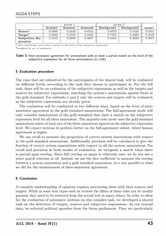
IGGSA-STEPS
group 1 group 2Armut1 Aussen1 Aussen2 Buchpreis1 Buchpreis2 mean2
Source1 0.5000 0.3448 0.6552 0.6970 0.7429 0.5811Target1 0.2000 0.2759 0.4483 0.7273 0.4000 0.4537Subjective Ex-pression
0.3155 0.2680 0.4987 0.4104 0.4829 0.3871
1only considering cases with a match on the level of the subjective expression2weighted by no. of sentences
Table 3: Inter-annotator agreement for annotations with at least a partial match on the level of thesubjective expression for all three annnotators (n=136)
5 Evaluation procedure
The runs that are submitted by the participants of the shared task, will be evaluatedon different levels, according to the task they choose to participate in. For the fulltask, there will be an evaluation of the subjective expressions as well as the targets andsources for subjective expressions, matching the system’s annotations against those inthe gold standard. For subtasks 1 and 2 only the sources and targets will be evaluated,as the subjective expressions are already given.The evaluation will be conducted in two different ways, based on the level of inter-
annotator agreement in the gold standard annotations: The full-agreement mode willonly consider annotations of the gold standard that have a match on the subjectiveexpression level for all three annotators. The majority-vote mode uses the gold standardannotations where at least two of the three annotators agreed on the subjective expressionlevel. We expect systems to perform better on the full-agreement subset, where humanagreement is higher.We use recall to measure the proportion of correct system annotations with respect
to the gold standard annotations. Additionally, precision will be calculated to give thefraction of correct system annotations with respect to all the system annotations. Forrecall and precision in both modes of evaluation, we recognize a match when thereis partial span overlap. Since full overlap on spans is relatively rare, we do not use astrict match criterion at all. Instead, we use the dice coefficient to measure the overlapbetween a system annotation and a gold standard annotation, in a way parallel to whatwe did for the measurement of inter-annotator agreement.
6 Conclusion
A complete understanding of opinions requires associating them with their sources andtargets. While in some text types such as reviews the fillers of these roles can be readilyguessed, they need to be retrieved from the actual text in many others. In order to allowfor the evaluation of automatic systems on this complex task, we developed a sharedtask on the detection of targets, sources and subjective expressions. As our textualdata, we selected political speeches from the Swiss parliament. They are particularly
JLCL 2014 – Band 29 (1) 43
Ruppenhofer, Struß, Sonntag, Gindl
suitable as they represent multiple topics, and contain multiple speakers and instancesof nesting.Using the guidelines that we developed through multiple rounds of annotation, we
achieved reasonably high inter-annotator agreement. We also presented how we planto evaluate the submissions of task participants. Our evaluation methods allow for aproper treatment of partial matches of annotation spans, and they distinguish cases ofperfect agreement among annotators from cases which a majority but not all annotatorslabeled. The shared task will be held in the run-up of the KONVENS conference in2014.
Acknowledgments
For their support in preparing and carrying out the annotations, we would like to thankJasper Brandes, Melanie Dick, Inga Hannemann, and Daniela Schneevogt.
Literature
Barbaresi, A. (2012). German Political Speeches, Corpus and Visualization. Technicalreport, ENS Lyon. 2nd Version.
Burchardt, A., Erk, K., Frank, A., Kowalski, A., and Pado, S. (2006). SALTO - AVersatile Multi-Level Annotation Tool. In Proceedings of the 5th Conference onLanguage Resources and Evaluation, pages 517–520.
Clematide, S., Gindl, S., Klenner, M., Petrakis, S., Remus, R., Ruppenhofer, J., Wal-tinger, U., and Wiegand, M. (2012). Mlsa - a multi-layered reference corpus forgerman sentiment analysis. In Calzolari, N., Choukri, K., Declerck, T., Do?an, M. U.,Maegaard, B., Mariani, J., Odijk, J., and Piperidis, S., editors, Proceedings of theEighth International Conference on Language Resources and Evaluation (LREC’12),Istanbul, Turkey. European Language Resources Association (ELRA).
Faaß, G. and Eckart, K. (2013). Sdewac – a corpus of parsable sentences from theweb. In Gurevych, I., Biemann, C., and Zesch, T., editors, Language Processing andKnowledge in the Web, volume 8105 of Lecture Notes in Computer Science, pages61–68. Springer Berlin Heidelberg.
Guerini, M., Strapparava, C., and Stock, O. (2008). Corps: A corpus of tagged politicalspeeches for persuasive communication processing. Journal of Information Technologyand Politics, 5(1):19–32.
Lezius, W. (2002). TIGERsearch - Ein Suchwerkzeug für Baumbanken. In Busemann,S., editor, Proceedings of KONVENS 2002, Saarbrücken, Germany.
44 JLCL

IGGSA-STEPS
Maks, I. and Vossen, P. (2011). A verb lexicon model for deep sentiment analysis andopinion mining applications. In Proceedings of the 2nd Workshop on Computatio-nal Approaches to Subjectivity and Sentiment Analysis (WASSA 2.0), pages 10–18,Portland, Oregon. Association for Computational Linguistics.
Nakov, P., Rosenthal, S., Kozareva, Z., Stoyanov, V., Ritter, A., and Wilson, T. (2013).SemEval-2013 Task 2: Sentiment Analysis in Twitter. In Second Joint Conference onLexical and Computational Semantics (*SEM), Volume 2: Proceedings of the SeventhInternational Workshop on Semantic Evaluation (SemEval 2013), pages 312–320,Atlanta and Georgia and USA. Association for Computational Linguistics.
Osenova, P. and Simov, K. (2012). The Political Speech Corpus of Bulgarian. In Chair),N. C. C., Choukri, K., Declerck, T., Doğan, M. U., Maegaard, B., Mariani, J., Odijk,J., and Piperidis, S., editors, Proceedings of the Eight International Conference onLanguage Resources and Evaluation (LREC’12), Istanbul, Turkey. European LanguageResources Association (ELRA).
Petrov, S. and Klein, D. (2007). Improved inference for unlexicalized parsing. In HumanLanguage Technologies 2007: The Conference of the North American Chapter of theAssociation for Computational Linguistics; Proceedings of the Main Conference, pages404–411, Rochester, New York. Association for Computational Linguistics.
Quirk, R., Greenbaum, S., Leech, G., and Svartvik, J. (1985). A comprehensive grammarof the English language. Longman.
Ruppenhofer, J., Somasundaran, S., and Wiebe, J. (2008). Finding the sources andtargets of subjective expressions. In LREC, Marrakech, Morocco.
Scherrer, Y. and Rambow, O. (2010). Natural language processing for the swiss germandialect area. In Pinkal, M., Rehbein, I., Schulte im Walde, S., and Storrer, A., editors,Semantic Approaches in Natural Language Processing, pages 93–102.
Schmid, H. (1994). Probabilistic part-of-speech tagging using decision trees. In Procee-dings of International Conference on New Methods in Language Processing, Manches-ter, UK.
Seki, Y., Evans, D., Ku, L.-W., Chen, H.-H., Kando, N., and Lin, C.-Y. (2007). Overviewof opinion analysis pilot task at ntcir-6. In Proceedings of NTCIR-6 Workshop Meeting,pages 265–278.
Seki, Y., Evans, D., Ku, L.-W., Sun, L., Chen, H.-H., Kando, N., and Lin, C.-Y. (2008).Overview of multilingual opinion analysis task at NTCIR-7. In Proceedings of the7th NTCIR Workshop Meeting on Evaluation of Information Access Technologies:Information Retrieval, Question Answering, and Cross-Lingual Information Access,pages 185–203.
JLCL 2014 – Band 29 (1) 45

Ruppenhofer, Struß, Sonntag, Gindl
Seki, Y., Ku, L.-W., Sun, L., Chen, H.-H., and Kando, N. (2010). Overview of Multi-lingual Opinion Analysis Task at NTCIR-8: A Step Toward Cross Lingual OpinionAnalysis. In Proceedings of the 8th NTCIR Workshop Meeting on Evaluation ofInformation Access Technologies: Information Retrieval, Question Answering andCross-Lingual Information Access, pages 209–220.
Stoyanov, V. and Cardie, C. (2008). Topic identification for fine-grained opinion analysis.In Proceedings of the 22nd International Conference on Computational Linguistics- Volume 1, COLING ’08, pages 817–824, Stroudsburg, PA, USA. Association forComputational Linguistics.
Strapparava, C. and Mihalcea, R. (2007). SemEval-2007 Task 14: Affective Text. InAgirre, E., Màrquez, L., and Wicentowski, R., editors, Proceedings of the FourthInternational Workshop on Semantic Evaluations (SemEval-2007), pages 70–74.Association for Computational Linguistics.
Thomas, M., Pang, B., and Lee, L. (2006). Get out the vote: Determining supportor opposition from Congressional floor-debate transcripts. In Proceedings of the2006 conference on empirical methods in natural language processing, pages 327–335.Association for Computational Linguistics.
Wiebe, J., Wilson, T., and Cardie, C. (2005). Annotating expressions of opinions andemotions in language. Language Resources and Evaluation, 39(2/3):164–210.
Wu, Y. and Jin, P. (2010). SemEval-2010 Task 18: Disambiguating Sentiment Ambi-guous Adjectives. In Erk, K. and Strapparava, C., editors, Proceedings of the 5thInternational Workshop on Semantic Evaluation, pages 81–85, Stroudsburg and PAand USA. Association for Computational Linguistics.
46 JLCL
JLCL 2014 – Band 29 (1) – 47-61
Kateřina Veselovská, Jan Hajič, jr., Jana Šindlerová
Subjectivity Lexicon for Czech: Implementation and Improvements
Abstract
The aim of this paper is to introduce the Czech subjectivity lexicon1, a new lexical resource
for sentiment analysis in Czech. We describe particular stages of the manual refinement of
the lexicon and demonstrate its use in the state-of-the art polarity classifiers, namely the
Maximum Entropy classifier. We test the success rate of the system enriched with the dic-
tionary on different data sets, compare the results and suggest some further improvements of
the lexicon-based classification system.
1 Introduction
Subjectivity lexicon generation is one of the tasks in sentiment analysis widely worked on
both in the academic and in the commercial sphere. The estimation of positive or negative
polarity is usually performed by detecting the polarity items, i.e. words or phrases inherently
bearing a positive or negative value. There are many methods for compiling a subjectivity
lexicon. One of the most straightforward ways is a translation (and further expansion) of an
already existing lexicon (see Section 2). Also, the list of evaluative items for specific do-
mains can be extracted directly from the evaluative data, either manually, or by use of prob-
abilistic models. However, it seems profitable for the polarity classification to combine both
manually annotated data and a set of the most frequent domain-independent polarity indica-
tors. In this article, we describe the results of an implementation of a method combining
classification trained on the reviews with polarity items from Czech subjectivity lexicon.
2 Related Work
The issue of building a subjectivity lexicon is generally described e.g. in (Taboada et al.,
2011) or (Liu, 2009). One of the earliest papers that is related to the collection of words with
polarity is (Hatzivassiloglou and McKeown, 1997). In their research they experimented with
adjectives of the same orientation of polarity. They identify and validate conjunction con-
straints with respect to the polarity of the adjectives they conjoin. Finally, they collected and
manually labelled 1,336 adjectives for their semantic orientation. The idea of words or
phrases that inherently bear certain polarity is also exploited in (Turney, 2002).
(Banea, Mihalcea and Wiebe, 2008) use a small set of subjectivity words and apply a
bootstrapping method of finding new candidates on the basis of a similarity measure. The
authors get to the number of 4000 top frequent entries for the final lexicon. They also de-
scribe another method for gaining a subjectivity lexicon: translation of an existing foreign
language subjectivity lexicon. Mostly, the authors employ subjectivity lexicons and senti-
ment analysis in general for machine translation purposes. They are interested e.g. in how
the information about polarity should be transferred from one language to another, if the
polarity could differ in the corresponding text spans and if it is possible to compile a subjec-
tivity lexicon for the target language during the translation.

JLCL 48
Veselovská, Hajič, Šindlerová
There are a number of papers dealing with the topic of building subjectivity lexicons for
particular languages (see e.g. Baklival et al., 2012, De Smedt et al., 2012, Jijkoun and Hof-
mann, 2009 or Peres-Rosas et al., 2012). Also, there is an ongoing research on sentiment
analysis in Czech, including the efforts to build a subjectivity lexicon (e.g. as part of a multi-
lingual system, see Steinberger et al., 2011). Still, as far as we know, there is no Czech
language subjectivity lexicon publicly available which would help to improve the task and
reach the state-of-the-art results.
3 Czech Subjectivity Lexicon
The core of the Czech subjectivity lexicon has been gained by automatic translation of a
freely available English subjectivity lexicon, also known as the Pittsburgh subjectivity clues,
introduced in (Wilson et al., 2005)2. The original lexicon, containing more than 8000 polari-
ty expressions, is a part of the OpinionFinder, the system for subjectivity detection in Eng-
lish. The clues in this lexicon were collected from a number of both manually and automati-
cally identified sources (see Riloff and Wiebe, 2003). The patterns and words are expanded
iteratively. Some scoring mechanisms were used to ensure the extracted words are in the
same semantic category as the seed words.
For translating the data to Czech, we only used parallel corpus CzEng 1.0 (Bojar and
Žabokrtský, 2006) containing 15 million parallel sentences (233 million English and 206
million Czech tokens) from seven different types of sources automatically annotated at
surface and deep layers of syntactic representation. By translation, we gained 7228 poten-
tially evaluative expressions. However, some of the items or the assigned polarities appeared
rather unreliable at first sight. For this reason, the lexicon has been manually surveyed by
one annotator and all the obviously non-evaluative items were excluded. In the end we
gained the first applicable version of the lexicon which contained 4947 evaluative expres-
sions. The most frequent items in this set were nouns (e.g. “hulvát” ‒ a boor, 1958) followed
by verbs (e.g. “mít rád” ‒ to like, 1699), adjectives (e.g. “špatný” ‒ bad, 821) and adverbs
(e.g. “dobře” ‒ rightly/well/correctly, 469).
3.1 Refining the Lexicon
After excluding clearly non-evaluative items, the lexicon has been manually checked again
for other incorrect entries. Below we mention the most significant types of inappropriate
entries, revealed in the checking phase by an experienced annotator.
The most common problem was including items that are evaluative only in a rare or in-
frequent meaning or in a specific semantic context whereas mostly they represent non-
evaluative expressions (e.g. “bouda” is in most cases used as a word for a “shed”, though it
can as well mean “dirty trick”). This concerns also the cases where the word is part of a
multi-word expression. The main criterion for marking the given item as evaluative was its
universal usability in a broader context. Thus we excluded most of the domain-dependent
items. The non-evaluativeness of the item was sometimes caused by wrong translation of the
original English expression. In case they had not been present in the lexicon yet, the correct
translations were added manually.

49
Subjectivity Lexicon for Czech
JLCL 2014 – Band 29 (1) 49
On the other hand, we found a lot of items with twofold polarity. These were mostly in-
tensifiers like “neuvěřitelně” (‘incredibly’), quantifiers like “moc” (‘a lot’), general modifi-
ers or words which are frequently connected both with positive and negative meaning (e.g.
“[dobré/špatné] svědomí” – [clear/guilty] conscience). The different polarities should be
distinguished later on by recording such words in the lexicon together with their prototypical
collocations. There are also other instances falling under this category of dual polarity, such
as ambiguous words which can be used both in positive and negative meaning – e.g. “využít
někoho”, meaning to abuse somebody (negative), and “využít příležitosti”, to take the op-
portunity (positive). We put these expressions aside for further research of their semantic
features and corpus analysis of their collocations, since they seem to be crucial for more
fine-grained sentiment analysis (see also Benamara et al., 2007).
Another problem concerns words assigned an incorrect polarity value. These could be di-
vided into several categories. One of them are e.g. diminutives marked with positive polarity
although they are very often used in negative (mostly ironic) sense – e.g. “svatoušek” –
goody-goody. Another large group consists of incorrect translations of negated words like
“nečestný” – not honest, “nemilosrdný” – not forgiving etc. In this case, the system did not
take into account the negative particle preceding the given word and assigned a positive
polarity.
After the manual refinement, we got 4,625 evaluative items altogether, of which 1,672
are positive, 2,863 are negative and 90 have both polarities assigned.
4 Evaluating the Lexicon
There are two basic ways to evaluate the quality of a subjectivity lexicon: looking directly at
the statistical properties of the lexicon, and plugging the lexicon into classification experi-
ments and measuring potential improvement it brings. We use datasets from various sources
and domains, with varying degree of annotation quality, to evaluate its usefulness in various
scenarios.
The lexicon can tell us whether a word encountered in the data has (or can have, or usual-
ly has) some polarity. We wish to evaluate how exact its estimate is and how useful it is for
polarity classification. This evaluation is twofold: while evaluating how accurate the lexicon
is, we are also evaluating how well human judgment on prior, context-less polarity of words
agrees with their usage and how much of evaluative language is actually expressed through
prototypical usage of words that humans judge by themselves evaluative.
Polarity (or, in a wider sense, subjectivity) disambiguation – deciding whether the given
token is polar – is a different topic; for the purposes of testing the lexicon, we assume that
for each lexicon entry, all its occurrences in the data are polar. By omitting a disambiguation
stage, we are estimating the upper bound on lexicon coverage of polar items (lexicon “re-
call”); disambiguating polar and neutral usage could, on the other hand, increase lexicon
“precision”.
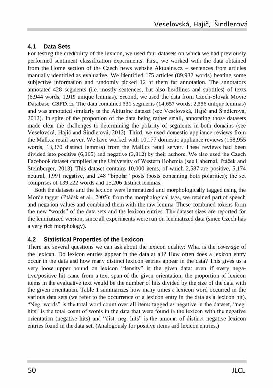
JLCL 50
Veselovská, Hajič, Šindlerová
4.1 Data Sets
For testing the credibility of the lexicon, we used four datasets on which we had previously
performed sentiment classification experiments. First, we worked with the data obtained
from the Home section of the Czech news website Aktualne.cz – sentences from articles
manually identified as evaluative. We identified 175 articles (89,932 words) bearing some
subjective information and randomly picked 12 of them for annotation. The annotators
annotated 428 segments (i.e. mostly sentences, but also headlines and subtitles) of texts
(6,944 words, 1,919 unique lemmas). Second, we used the data from Czech-Slovak Movie
Database, CSFD.cz. The data contained 531 segments (14,657 words, 2,556 unique lemmas)
and was annotated similarly to the Aktualne dataset (see Veselovská, Hajič and Šindlerová,
2012). In spite of the proportion of the data being rather small, annotating those datasets
made clear the challenges to determining the polarity of segments in both domains (see
Veselovská, Hajič and Šindlerová, 2012). Third, we used domestic appliance reviews from
the Mall.cz retail server. We have worked with 10,177 domestic appliance reviews (158,955
words, 13,370 distinct lemmas) from the Mall.cz retail server. These reviews had been
divided into positive (6,365) and negative (3,812) by their authors. We also used the Czech
Facebook dataset compiled at the University of Western Bohemia (see Habernal, Ptáček and
Steinberger, 2013). This dataset contains 10,000 items, of which 2,587 are positive, 5,174
neutral, 1,991 negative, and 248 “bipolar” posts (posts containing both polarities); the set
comprises of 139,222 words and 15,206 distinct lemmas.
Both the datasets and the lexicon were lemmatized and morphologically tagged using the
Morče tagger (Ptáček et al., 2005); from the morphological tags, we retained part of speech
and negation values and combined them with the raw lemma. These combined tokens form
the new “words” of the data sets and the lexicon entries. The dataset sizes are reported for
the lemmatized version, since all experiments were run on lemmatized data (since Czech has
a very rich morphology).
4.2 Statistical Properties of the Lexicon
There are several questions we can ask about the lexicon quality: What is the coverage of
the lexicon. Do lexicon entries appear in the data at all? How often does a lexicon entry
occur in the data and how many distinct lexicon entries appear in the data? This gives us a
very loose upper bound on lexicon “density” in the given data: even if every nega-
tive/positive hit came from a text span of the given orientation, the proportion of lexicon
items in the evaluative text would be the number of hits divided by the size of the data with
the given orientation. Table 1 summarizes how many times a lexicon word occurred in the
various data sets (we refer to the occurrence of a lexicon entry in the data as a lexicon hit).
“Neg. words” is the total word count over all items tagged as negative in the dataset, “neg.
hits” is the total count of words in the data that were found in the lexicon with the negative
orientation (negative hits) and “dist. neg. hits” is the amount of distinct negative lexicon
entries found in the data set. (Analogously for positive items and lexicon entries.)

51
Subjectivity Lexicon for Czech
JLCL 2014 – Band 29 (1) 51
Dataset Neg. words Pos. words Neg. hits Dist. neg. hits Pos. hits Dist. pos. hits
Aktualne 1003 358 119 53 102 59
CSFD 4739 6231 254 68 301 65
Reviews 60652 98303 1676 154 4174 146
Facebook 33091 30361 1166 186 2661 182
Tab. 1: Lexicon coverage
However, since many lexicon hits are not in the text span of the corresponding polarity,
we need to proceed to testing how good the lexicon is as a predictor. To this end, we used a
series of primitive, “raw” binary classifiers. Note that these classifiers are just helper con-
structs for measuring the relationship between lexicon hits and data item orientations.
We define lexicon features: the counts of positive and the count of negative items from
the lexicon in the text span. We will call the features POS and NEG. If a lexicon item per-
mits both polarities, it contributes both to POS and NEG counts. If the text span contained
no lexicon item, it was given a technical NTR feature with count 1.
We then derive lexicon indicator variables from lexicon features: if a lexicon feature is
greater or equal to some threshold frequency (denoted thresholdLI, by default 1) for a data
item, the indicator variable value for the given data item is 1; otherwise it is 0. We will
denote these features as LIPOS, LINEG and LINTR (LI = Lexicon Indicator).
The raw negative classifier then labels all items with negative hits – those with a LINEG
value of 1 – as negative and all the others as non-negative. These binary “predictions” then
are evaluated against the binarized “true classes” – all negative data items receive a 1, all
non-negative a 0. Analogously for positive items. (Note that under this scheme, one data
item may receive a 1 for multiple lexicon indicator features – if it contains both a negative
and a positive lexicon hit; this would be a concern if we were building a classifier for all
classes at once. However, it only has one true orientation, so it can only contribute once to a
correct classification.)
The raw neutral classifier labels as neutral items without more than thresholdLI lexicon
hits. The “both” class is not predicted.
For each raw classifier on each dataset, we report its precision, recall and support (the
true number of data items with the given polarity label) for the label of interest (NEG for the
raw negative classifiers, etc.). Recall is the ratio of text spans of the given polarity “found”
by the lexicon to the total amount of data items labelled with this polarity, precision is the
proportion of correctly identified data items in the set. A recall of 0.5 for the label NEG and
negative polarity data items means that in half of the negative data items, a negative lexicon
entry appeared. A precision 0.5 means that half the data items in which a negative lexicon
entry appeared are actually items labelled as negative in the data.
Given that we are building a separate raw classifier for each class, the baseline perfor-
mance is also computed for each class separately. The baseline classification assigns a 1 to
the LI feature for each data item. This simulates the situation of a lexicon which tags at least
one word in every item with the given orientation. Baseline recall is thus 1.0 and so recall
ceases to be of interest; our focus is precision, which will tell us how well the lexicon hits

JLCL 52
Veselovská, Hajič, Šindlerová
are able to signal that an item actually has the orientation they indicate. At the same time,
we watch recall to see a more detailed overview of lexicon coverage.
Recall and precision the raw classifiers achieved are captured in Table 2.
Dataset Target label Recall Precision Baseline p. Support
Aktualne POS 0.294 0.054 0.040 17
NEG 0.324 0.230 0.166 71
NTR 0.598 0.792 0.792 338
CSFD POS 0.454 0.451 0.345 183
NEG 0.377 0.333 0.284 151
NTR 0.579 0.467 0.371 197
Reviews POS 0.354 0.744 0.639 6500
NEG 0.204 0.551 0.361 3677
NTR 0.000 0.000 0.000 0
Facebook POS 0.278 0.320 0.259 2587
NEG 0.162 0.298 0.199 1991
NTR 0.741 0.554 0.517 5174
Tab. 2: Lexicon feature “raw” performance
The most important finding from Table 2 is that raw classifier precision tends to follow
the baseline for the given label (the proportion of text spans of that class in the data)3. This
means that the presence or absence of lexicon words per se gives us no additional infor-
mation: if a lexicon word were present in every data item, we would have the same precision.
Setting thresholdLI to 2 very predictably slightly improves precision (at most on the order
of 0.1) while drastically reducing recall (to between 0.03 and 0.1). Setting the threshold to 3
showed that no neutral item contained 3 or more lexicon hits and very few non-neutral items
did.
While precision can be improved by using more sophisticated classification methods, re-
call is more limiting – if only 65 % of positive items contain a positive lexicon item, unless
we are able to generalize from the lexicon to unseen words, we simply cannot improve recall
over 0.65 unless we expand the lexicon.
Again, note that feature performance as measured above is not the performance of “real”
classifiers using the lexicon features. The raw classifiers are among the most unsophisticated
classification methods based on the lexicon; however, they set a lower bound on what
should definitely be achievable with the lexicon, based on how lexicon words occur in or
outside items with corresponding orientations.
4.3 Evaluation against annotated polar expressions
Since the Aktualne and CSFD data sets are annotated at the expression level4 including
explicitly tagged polar expressions (parts of data items that make the annotator believe the
item contains an evaluation, see (Veselovská, Hajič jr. and Šindlerová 2012) for details), we
can measure how much the lexicon hits correlate with these expressions. In this polar
expression data, there are naturally only positive and negative data items, since only in them

53
Subjectivity Lexicon for Czech
JLCL 2014 – Band 29 (1) 53
the polar expressions were annotated. We again measure precision, which in this case is the
proportion of hits that occur inside polar expressions to the total amount of hits, and recall,
which is the proportion of polar expressions with lexicon hits to the number of all polar
expressions. The results are reported in Table 3. In this case, support is the number of polar
expressions annotated with the given orientation by the given annotator. Since the polar
expressions were tagged by two annotators with both significant overlap and significant
differences, we report precision and recall for annotators separately (annotator 1/annotator
2).
Dataset Orientation Recall Precision Support
Aktualne POS 0.15/0.24 0.50/0.67 13/17
NEG 0.26/0.26 1.00/0.94 58/66
CSFD POS 0.09/0.14 0.72/0.87 194/143
NEG 0.09/0.10 0.78/0.82 152/138
Tab. 3: Precision and Recall against annotated polar expressions
While recall is still low, if the lexicon identifies something, it does tend to lie in expressions
of the corresponding orientation. This again suggests that a disambiguation stage is in order;
once we know the lexicon hit lies in an evaluative statement, the hit orientation can be relied
upon
4.4 Evaluation within Classification Experiments
A further way of testing the lexicon is using lexicon features directly in a classification task,
comparing them to automatically extracted features (word and n-gram counts) and
evaluating also the combination of automatic and lexicon features. Contrary to the
precision/recall scores reported above, the results reported here are for “real” classifiers that
classify items by orientation, so that the NEG, NTR, POS and BOTH labels are generated at
once. (In section 4.2, each raw classifier was a separate entity.)
Automatic features used in classification were simply word counts. The value of feature f
in a text span represents how many times the lemma corresponding to feature f was present.
All classification experiments report 5-fold cross-validation averages. We used the
MaxEnt classifier (implemented as Logistic Regression in the scikit-learn Python library5 ).
The regularization parameter was set to 1.0 with the exception of the Aktualne dataset,
where setting it to values of several thousand significantly improves the performance on the
positive text spans.
We report results for the individual classes. It is more informative, especially for datasets
with large imbalances of classes, than to report the averaged performance. (Since the classi-
fier performance was never significantly changed by including the lexicon features, the
results are reported for classification with automatic and combined lexicon/automatic fea-
tures in the same table.)
Table 4 shows the results on the Aktualne dataset (note that given the small size and
heavily imbalanced nature of the dataset, the results for the negative and positive classes
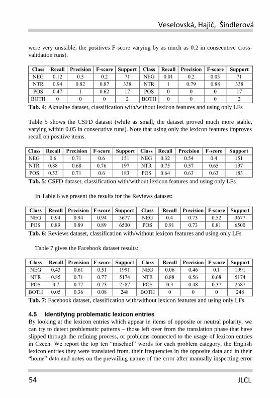
JLCL 54
Veselovská, Hajič, Šindlerová
were very unstable; the positives F-score varying by as much as 0.2 in consecutive cross-
validation runs).
Class Recall Precision F-score Support Class Recall Precision F-score Support
NEG 0.12 0.5 0.2 71 NEG 0.01 0.2 0.03 71
NTR 0.94 0.82 0.87 338 NTR 1 0.79 0.88 338
POS 0.47 1 0.62 17 POS 0 0 0 17
BOTH 0 0 0 2 BOTH 0 0 0 2 Tab. 4: Aktualne dataset, classification with/without lexicon features and using only LFs
Table 5 shows the CSFD dataset (while as small, the dataset proved much more stable,
varying within 0.05 in consecutive runs). Note that using only the lexicon features improves
recall on positive items.
Class Recall Precision F-score Support Class Recall Precision F-score Support
NEG 0.6 0.71 0.6 151 NEG 0.32 0.54 0.4 151
NTR 0.88 0.68 0.76 197 NTR 0.75 0.57 0.65 197
POS 0.53 0.71 0.6 183 POS 0.64 0.63 0.63 183 Tab. 5: CSFD dataset, classification with/without lexicon features and using only LFs
In Table 6 we present the results for the Reviews dataset:
Class Recall Precision F-score Support Class Recall Precision F-score Support
NEG 0.94 0.94 0.94 3677 NEG 0.4 0.73 0.52 3677
POS 0.89 0.89 0.89 6500 POS 0.91 0.73 0.81 6500 Tab. 6: Reviews dataset, classification with/without lexicon features and using only LFs
Table 7 gives the Facebook dataset results:
Class Recall Precision F-score Support Class Recall Precision F-score Support
NEG 0.43 0.61 0.51 1991 NEG 0.06 0.46 0.1 1991
NTR 0.85 0.71 0.77 5174 NTR 0.88 0.56 0.68 5174
POS 0.7 0.77 0.73 2587 POS 0.3 0.48 0.37 2587
BOTH 0.05 0.36 0.08 248 BOTH 0 0 0 248 Tab. 7: Facebook dataset, classification with/without lexicon features and using only LFs
4.5 Identifying problematic lexicon entries
By looking at the lexicon entries which appear in items of opposite or neutral polarity, we
can try to detect problematic patterns – those left over from the translation phase that have
slipped through the refining process, or problems connected to the usage of lexicon entries
in Czech. We report the top ten “mischief” words for each problem category, the English
lexicon entries they were translated from, their frequencies in the opposite data and in their
“home” data and notes on the prevailing nature of the error after manually inspecting error
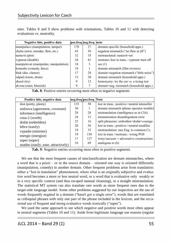
55
Subjectivity Lexicon for Czech
JLCL 2014 – Band 29 (1) 55
sites. Tables 8 and 9 show problems with orientations, Tables 10 and 11 with detecting
evaluations vs. neutrality.
Negative hits, positive data pos.freq neg.freq note
manipulace (manipulation, tamper)
chyba (error, mistake, flaw, etc.)
nastavit (plot)
vypnout (disable)
manipulovat (manipulate, manipulation)
komedie (comedy, farce)
hluk (din, clamor)
odpad (waste, drain)
zkusit (try)
skvrna (stain, blemish)
178
65
32
24
18
18
17
13
9
9
27
56
35
41
3
1
28
20
12
7
domain-specific (household apps.)
negation mismatch (“no flaw at all”)
mistranslated: nastavit=set
mistrans./lost in trans.: vypnout=turn off
see (1)
domain mismatch (film reviews)
domain+negation mismatch (“little noise”)
domain mismatch (household apps.)
homonymy: try the car vs. a trying test
domain+neg. mismatch (household apps.) Tab. 8: Positive entries occurring most often in negative segments
Positive hits, negative data neg.freq pos.freq Note
dost (pretty, plenty)
smlouva (agreement, covenant)
informace (intelligence)
cena-2 (worth)
dodat (embolden)
lehce (easily)
vypadat (minister)
energie (energize)
super (super)
snadno (easily, ease, attractively)
135
30
28
24
22
20
19
19
17
16
58
1
28
12
16
56
35
158
127
69
lost in trans.: positive->neutral intensifier
domain mismatch (phone operator trouble)
mistranslation (intelligence as in CIA)
lemmatization disambiguation error
split phraseme: embolden=dodat+courage
lost in trans.: positive->neutral modifier
mistranslation: rare Eng. to common Cz.
lost in trans.+mistrans.: wrong POS
irony/sarcasm + adversative constructions
analogous to (6)
Tab. 9: Negative entries occurring most often in positive segments
We see that the most frequent causes of misclassification are domain mismatches, where
a word that is a priori – or in the source domain – oriented one way is oriented differently
(manipulation, comedy) in another domain. Other frequent problems arise from translation:
either a “lost in translation” phenomenon, where what is an originally subjective and evalua-
tive word becomes a more or less neutral word, or a word that is evaluative only weakly or
in a very specific context (and thus escaped manual cleansing), or a straight mistranslation.
The statistical MT system can also translate rare words as more frequent ones due to the
target-side language model. Some other problems suggested by our inspection are the use of
words frequently negated in a domain (“hasn't got a single error”), words that are translated
as colloquial phrases with only one part of the phrase included in the lexicon, and the occa-
sional use of frequent and strong evaluative words ironically (“super”).
We used the same approach to see which negative and positive words most often appear
in neutral segments (Tables 10 and 11). Aside from legitimate language use reasons (regular

JLCL 56
Veselovská, Hajič, Šindlerová
non-evaluative usage), the discovery of which is again a task for disambiguating whether an
entry is used as an evaluative word, the most frequent problems stemmed from translation.
Negative hits, neutral data ntr.freq neg.freq note
zkusit (try, difficult)
chyba (error, mistake, failure, flaw...)
situace (crisis, predicament, plight...)
nastavit (plot)
chybit (miss)
ztratit (lose, vanish, doom, dishearten)
smrt (death, martyrdom, dying)
zmizet (vanish, abscond, swagger)
vypnout (disable)
sranda (fun, goof)
48
46
17
17
16
12
11
9
9
9
12
56
7
2
2
1
2
5
41
7
homonymy: try the car vs. a trying test
regular non-evaluative usage of “chyba”
lost in translation: crisis->situation
mistranslated: nastavit = set
see (2)
regular non-evaluative usage of “lose”
regular non-evaluative usage of “death”
lost in translation: “zmizet” is neutral
lost in translation: “vypnout” = “turn off”
orientation error in lexicon refinement Tab. 10: Negative entries occurring most often in neutral segments
Positive hits, neutral data ntr.freq pos.freq note
cena (worth)
doufat (hope, hopefully, hopefulness)
vypadat (minister)
informace (intelligence)
dost (pretty, plenty)
dobro (good)
souhlasit (agree, consent, concur...)
smlouva (agreement, covenant)
radost (joy, pleasure, delight, happines...)
chystat (solace)
40
36
30
29
28
27
21
20
15
14
12
32
35
28
56
42
15
1
33
6
lemmatization disambiguation error
lost in translation: neutral colloquial usage
mistranslation: rare Eng. to common Cz.
mistranslation: rare Eng. to common Cz.
lost in trans.: positive->neutral modifier
phrase “dobrý den“ (greeting phrase)
regular non-evaluative usage of “agree”
domain mismatch (cell phone operators)
non-eval. usage, misannotated items
mistranslation: “chystat” = “to prepare” Tab. 11: Positive entries occurring most often in neutral segments
4.6 Automated lexicon pruning
Since the number of incorrect hits drops off roughly exponentially, we hypothesised that
we could significantly improve lexicon indicator precision by pruning. To see how much we
could gain by removing misleading lexicon entries, we combined half of the Facebook and
Reviews data to find lexicon entries that impede classification. We then computed the recall
and precision statistics of lexicon indicator features and coverage statistics on the second
halves of the data (see Fig. 1).
An entry was classified as misleading if we couldn't reject the hypothesis that its occur-
rences are evenly distributed across items of its class vs. items of all other classes combined,
or if we could reject this hypothesis and it occurred less frequently in items of its class than
in other items. We used the binomial exact test since lexicon hits are often low-frequency
words and we thus cannot accurately use the chi-square test.
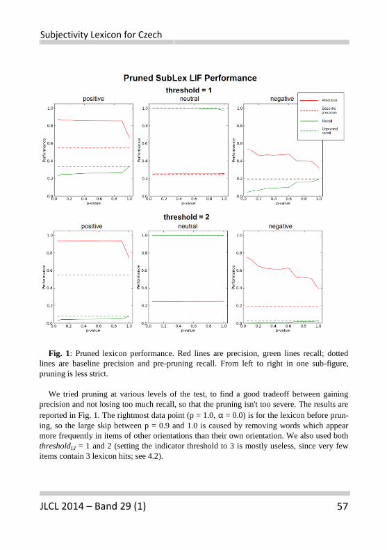
57
Subjectivity Lexicon for Czech
JLCL 2014 – Band 29 (1) 57
Fig. 1: Pruned lexicon performance. Red lines are precision, green lines recall; dotted
lines are baseline precision and pre-pruning recall. From left to right in one sub-figure,
pruning is less strict.
We tried pruning at various levels of the test, to find a good tradeoff between gaining
precision and not losing too much recall, so that the pruning isn't too severe. The results are
reported in Fig. 1. The rightmost data point (p = 1.0, α = 0.0) is for the lexicon before prun-
ing, so the large skip between p = 0.9 and 1.0 is caused by removing words which appear
more frequently in items of other orientations than their own orientation. We also used both
thresholdLI = 1 and 2 (setting the indicator threshold to 3 is mostly useless, since very few
items contain 3 lexicon hits; see 4.2).

JLCL 58
Veselovská, Hajič, Šindlerová
The very low recall for some classes meant that less than 10 items actually contained a
lexicon hit of their polarity. However, after such automated pruning, the lexicon may be
suitable for building a high-precision classifier such as in (Riloff and Wiebe, 2003).
On the Aktualne dataset, the pruned lexicon never achieved higher precision than the un-
pruned version. However, on the CSFD data set, for p = 0.05 and, thresholdLI = 2, the preci-
sion for LIPOS defeated the unpruned (0.793 vs. 0.543) with precision for the other indicators
not significantly different from the unpruned lexicon scores.
5 Conclusions and Future Work
From the experiment with lexicon feature recall and precision, we believe that a disambigua-
tion stage, where the occurrence of a lexicon item is assigned some confidence that the
occurrence actually is polar, could be highly beneficial – words from the lexicon frequently
appear in text spans of opposite polarities or neutral text spans.
Adding the lexicon features to sentiment classifiers did not significantly improve the re-
sults in any experiment we have run so far, with the exception of positive text spans in the
CSFD dataset. Using the lexicon features alone, which is an option in a scenario where
manually annotated data is not available, might work decently on the datasets with preemi-
nently evaluative user-generated content: Aktualne and CSFD. However, to confirm this
claim it would be useful to repeat the experiments using other classifiers.
As for the general usefulness of the lexicon, it is apparent that the lexicon by itself – at
least by using lexicon features in the manner described above – cannot compete with statis-
tical methods on a representative in-domain annotated dataset such as Reviews, and even
when the automatic features are combined with the lexicon features, classifier performance
does not improve. However, the lexicon does not hurt classification either, and it remains to
be seen whether it can help in classifying previously unseen domains (the Aktualne and
CSFD datasets are not large enough for conclusive testing), although the prevalence of
domain mismatch among frequent causes of entry/data item orientation mismatch suggests
that this will at least require a more sophisticated method.
In order to improve the automatic polarity classification, it could also be advantageous to
enhance the subjectivity lexicon by several methods. Firstly, we could use the dictionary-
based approach as described by Hu and Liu (2004) or Kim and Hovy (2004) and grow the
basic set of words by searching for their synonyms in Czech WordNet (Pala and Ševeček,
1999).
Secondly, we could employ the corpus-based approach based on syntactic or co-
occurrence patterns as described in (Hatzivassiloglou & McKeown, 1997). Also, we can
extend the lexicon manually by Czech evaluative idioms and other common evaluative
phrases. Moreover, it would be useful to add back some special domain-dependent modules
for the different areas of evaluation.
To improve the lexicon itself by automatic means besides pruning by statistical signifi-
cance, we can “ablate” the lexicon: try removing features and see how much the removal
hurts (or helps) classification in various scenarios both already implemented and new.

59
Subjectivity Lexicon for Czech
JLCL 2014 – Band 29 (1) 59
6 Acknowledgments
The research described herein has been supported by the by SVV project number 260 140
and by the LINDAT/CLARIN project funded by the Ministry of Education, Youth and
Sports of the Czech Republic, project No. LM2010013.
This work has been using language resources developed and/or stored and/or distributed
by the LINDAT/CLARIN project of the Ministry of Education, Youth and Sports of the
Czech Republic (project LM2010013). 1 Available at http://ufal.mff.cuni.cz/seance/data.
2Available at http://www.cs.pitt.edu/mpqa/subj_lexicon.html. 3 This is the same result we could get for evaluative text spans by tagging each with every fea-ture. However, we avoid this degenerate case by also reporting statistics for neutral text spans, if available. 4 We derived a segment-level polarity from the expression-level annotations.
5Available at http://scikit-learn.org/stable. For experiments with machine learning, the library has
proven to be for us an excellent tool.
References
BAKLIWAL, A., ARORA, P., AND VARMA, V. (2012). "Hindi subjective lexicon: A
lexical resource for hindi adjective polarity classification". In Proceedings of the Eight
International Conference on Language Resources and Evaluation (LREC’12), Chair K.
Choukri, T. Declerck, M. U. Dogan, B. Maegaard, J. Mariani, J. Odijk, and S. Piperidis,
Eds., European Language Resources Association (ELRA).
BANEA, C., MIHALCEA, R., AND WIEBE, J. (2008). "A bootstrapping method for
building subjectivity lexicons for languages with scarce resources". In Proceedings of LREC
(2008).
BANEA, C., MIHALCEA, R., WIEBE, J. AND HASSAN, S. (2008). "Multilingual subjec-
tivity analysis using machine translation". In Proceedings of the Conference on Empirical
Methods in Natural Language Processing (pp. 127-135). Association for Computational
Linguistics.
BENAMARA, F., CESARANO, C. AND REFORGIATO, D. (2007). "Sentiment analysis:
Adjectives and adverbs are better than adjectives alone". Proceedings of the International
Conference on Weblogs and Social Media (ICWSM).

JLCL 60
Veselovská, Hajič, Šindlerová
BOJAR, O. AND ŽABOKRTSKÝ, Z. (2006). "CzEng: Czech-English Parallel Corpus,
Release version 0.5". Prague Bulletin of Mathematical Linguistics, 86. Available
from http://ufal.mff.cuni.cz/czeng/.
DE SMEDT, T. AND W. DAELEMANS (2012). "Vreselijk mooi! (terribly beautiful): A
subjectivity lexicon for dutch adjectives". In Proceedings of the 8th Language Resources
and Evaluation Conference (LREC'12).
HABERNAL, I., PTÁČEK, T. AND STEINBERGER, J. (2013). "Sentiment Analysis in
Czech Social Media Using Supervised Machine Learning". WASSA 2013: 65.
HATZIVASSILOGLOU, V. AND MCKEOWN, K. R. (1997). "Predicting the semantic
ori-entation of adjectives". Proceedings of the eighth conference on European chapter of the
Association for Computational Linguistics. Association for Computational Linguis-tics.
HU, M., AND LIU, B. (2004). "Mining and summarizing customer reviews." Pro-
ceedings of the tenth ACM SIGKDD international conference on Knowledge discovery and
data mining. ACM, 2004.
JIJKOUN, V. AND HOFMANN, K. (2009). "Generating a Non-English Subjectivity
Lexicon: Relations That Matter". In proceeding of: EACL 2009, 12th Conference of the
European Chapter of the Association for Computational Linguistics, Proceedings of the
Conference.
KIM, S.-M., AND HOVY, E. (2004). "Determining the sentiment of opinions." Pro-
ceedings of the 20th international conference on Computational Linguistics. Association for
Computational Linguistics.
LIU, B. (2009). "Sentiment Analysis and Subjectivity". Invited Chapter for the
Handbook of Natural Language Processing, Second Edition. Marcel Dekker, Inc: New York.
PALA, K. AND ŠEVEČEK, P. (1999). "The Czech WordNet, final report". Brno: Ma-
sarykova univerzita.
PEREZ-ROSAS, V., BANEA, C. AND MIHALCEA, R. (2012). "Learning Sentiment Lex-
icons in Spanish". In Proceedings of the 8th international conference on Language Re-
sources and Evaluation (LREC2012).
RILOFF, E. AND WIEBE, J. (2003). "Learning extraction patterns for subjective ex-
pressions". In Proceedings of EMNLP-2003.

61
Subjectivity Lexicon for Czech
JLCL 2014 – Band 29 (1) 61
STEINBERGER, J., LENKOVA, P., KABADJOV, M., STEINBERGER, R. AND VAN DER
GOOT, E. (2011). "Multilingual Entity-Centered Sentiment Analysis Evaluated by Parallel
Corpora". In Proceedings of the 8th International Conference Recent Advances in Natural
Language Processing.
TABOADA, M., BROOKS, J., TOFILOSKI, M., VOLL, K. AND STEDE, M. (2011). "Lexi-
con-Based Methods for Sentiment Analysis". Computational Linguistics, 37(2), pp. 267-307.
TURNEY, P. D. (2002). "Thumbs up or thumbs down?: semantic orientation applied
to unsupervised classification of reviews". In Proceedings of the 40th annual meeting on
association for computational linguistics, Association for Computational Linguistics, pp.
417–424.
VESELOVSKÁ, K., HAJIČ JR., J. AND ŠINDLEROVÁ, J. (2012). "Creating Annotated
Resources for Polarity Classification in Czech". In Proceedings of the 11th Conference on
Natural Language Processing, Schriftenreihe der Österreichischen Gesellschaft für Artificial
Intelligende (ÖGAI), Vienna, Austria, 2012
WILSON, T., WIEBE, J., AND HOFFMANN, P. (2005). "Recognizing contextual polari-
ty in phrase-level sentiment analysis". In Proceedings of HLT/EMNLP 2005.

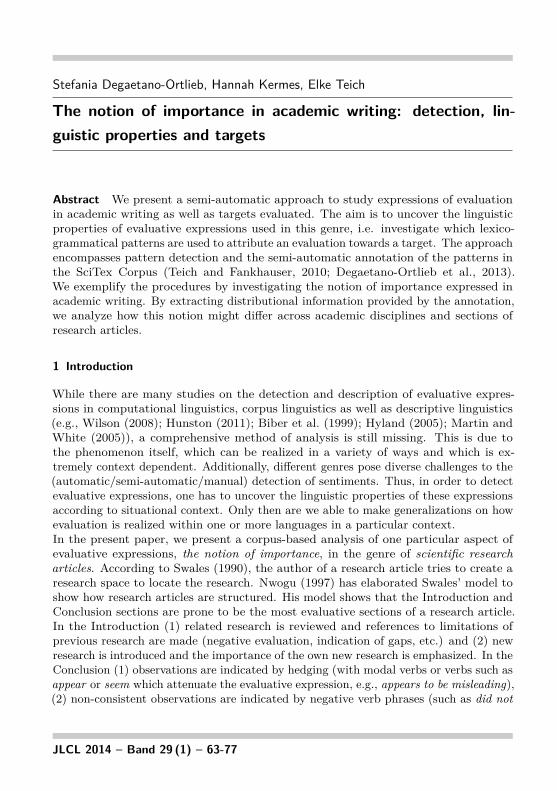
Stefania Degaetano-Ortlieb, Hannah Kermes, Elke Teich
The notion of importance in academic writing: detection, lin-guistic properties and targets
Abstract We present a semi-automatic approach to study expressions of evaluationin academic writing as well as targets evaluated. The aim is to uncover the linguisticproperties of evaluative expressions used in this genre, i.e. investigate which lexico-grammatical patterns are used to attribute an evaluation towards a target. The approachencompasses pattern detection and the semi-automatic annotation of the patterns inthe SciTex Corpus (Teich and Fankhauser, 2010; Degaetano-Ortlieb et al., 2013).We exemplify the procedures by investigating the notion of importance expressed inacademic writing. By extracting distributional information provided by the annotation,we analyze how this notion might differ across academic disciplines and sections ofresearch articles.
1 Introduction
While there are many studies on the detection and description of evaluative expres-sions in computational linguistics, corpus linguistics as well as descriptive linguistics(e.g., Wilson (2008); Hunston (2011); Biber et al. (1999); Hyland (2005); Martin andWhite (2005)), a comprehensive method of analysis is still missing. This is due tothe phenomenon itself, which can be realized in a variety of ways and which is ex-tremely context dependent. Additionally, different genres pose diverse challenges to the(automatic/semi-automatic/manual) detection of sentiments. Thus, in order to detectevaluative expressions, one has to uncover the linguistic properties of these expressionsaccording to situational context. Only then are we able to make generalizations on howevaluation is realized within one or more languages in a particular context.In the present paper, we present a corpus-based analysis of one particular aspect ofevaluative expressions, the notion of importance, in the genre of scientific researcharticles. According to Swales (1990), the author of a research article tries to create aresearch space to locate the research. Nwogu (1997) has elaborated Swales’ model toshow how research articles are structured. His model shows that the Introduction andConclusion sections are prone to be the most evaluative sections of a research article.In the Introduction (1) related research is reviewed and references to limitations ofprevious research are made (negative evaluation, indication of gaps, etc.) and (2) newresearch is introduced and the importance of the own new research is emphasized. In theConclusion (1) observations are indicated by hedging (with modal verbs or verbs such asappear or seem which attenuate the evaluative expression, e.g., appears to be misleading),(2) non-consistent observations are indicated by negative verb phrases (such as did not
JLCL 2014 – Band 29 (1) – 63-77

Degaetano-Ortlieb, Kermes, Teich
reveal) or negative quantifiers, (3) overall research outcomes are highlighted by prepara-tory statements (e.g., the results suggest that/offer clear evidence that), and (4) specificresearch outcomes are explained by lexical items signaling significance/importance (e.g.,results are important) and by preparatory statements to indicate limitations of previousstudies (e.g., error, clearly unable, did not mention). From these observations, one canthink of (a) possible expressions of evaluation involved in academic writing (such asimportance/significance) and (b) possible targets the evaluation is directed towards(such as previous/own research, observations, outcomes, etc.).According to Hunston and Francis (2000) expressions of evaluation towards a target canbe expressed by evaluative patterns, i.e. lexico-grammatical structures that attribute anevaluation to a target. Here, we can have strictly evaluative patterns, such as it BE ADJto/that, where the ADJ position is always filled with an evaluative adjective, or patternsthat are possibly evaluative, such as the importance of linear problem kernels, wherethe noun preceding the of-phrase can have an evaluative meaning such as importancein this case. Clearly, it is not possible to detect all instances of evaluative language bystructural patterns. However, the pattern approach allows a fairly systematic way ofidentification of particular evaluative expressions in large corpora, supporting a morecomprehensive picture of the linguistic properties involved in evaluation.To detect these patterns and targets, we rely on a corpus-based approach that involvesdetection of evaluative patterns and pattern annotation. Having the corpus annotated,we can analyze differences between disciplines in terms of evaluative expressions andexplore the linguistic properties of specific evaluative ‘modes’ in academic writing,such as evaluative meanings (e.g., importance, obviousness, complexity) and evaluativeattribution structures, i.e. whether the evaluative expression precedes the target (pre-evaluation, e.g., the [eval importance] of [target linear problem kernels]) or follows thetarget (post-evaluation, e.g., [target A] [eval fails] to be a BPP algorithm) or whethera relational structure is used to attribute the evaluation to the target (e.g., [eval Onecrucial issue] [rel is] [target that of stability]). Our main goal is to examine the linguisticproperties of evaluative expressions of importance and to see whether they differ acrossacademic disciplines and document sections. We address the following questions: Whichlexical units are used to express importance? Which are the linguistic properties ofexpressions of importance, i.e. which lexico-grammatical patterns are used? Whichkinds of targets are evaluated and are there differences across disciplines and sectionsof research articles?The paper is structured as follows: In Section 2, we describe the data and the methodol-ogy applied. Section 3 presents the analysis of importance in academic writing. Section4 concludes the paper with a summary and an envoi.
64 JLCL
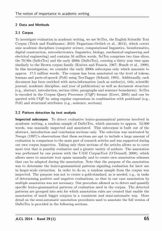
The notion of importance in academic writing
2 Data and Methods
2.1 Corpus
To investigate evaluation in academic writing, we use SciTex, the English Scientific TextCorpus (Teich and Fankhauser, 2010; Degaetano-Ortlieb et al., 2013), which coversnine academic disciplines (computer science, computational linguistics, bioinformatics,digital construction, microelectronics, linguistics, biology, mechanical engineering andelectrical engineering) and contains 34 million words. SciTex comprises two time slices,the 70/80s (SaSciTex) and the early 2000s (DaSciTex), covering a thirty year time spansimilarly to the Brown corpus family (Kučera and Francis, 1967; Hundt et al., 1999).In this investigation, we consider the early 2000s subcorpus only which amounts toapprox. 17.5 million words. The corpus has been annotated on the level of tokens,lemmas and parts-of-speech (PoS) using TreeTagger (Schmid, 1994). Additionally, eachdocument has been enriched with meta-information (such as author(s), title, scientificjournal, academic discipline, and year of publication) as well as document structure(e.g., abstract, introduction, section titles, paragraphs and sentence boundaries). SciTexis encoded in the Corpus Query Processor (CQP) format (Evert, 2005) and can bequeried with CQP by using regular expressions in combination with positional (e.g.,PoS) and structural attributes (e.g., sentence, sections).
2.2 Pattern detection by text analysis
Inspected subcorpus To detect evaluative lexico-grammatical patterns involved inacademic writing, a random sample of DaSciTex, which amounts to approx. 52.000words, was manually inspected and annotated. This subcorpus is built out of theabstract, introduction and conclusion sections only. The selection was motivated byNwogu (1997)’s observations that these sections are apt to include a large amount ofevaluation in comparison to the main part of research articles and was supported duringour own corpus inspection. Taking only these sections of the articles allows us to covermore text that is possibly evaluative and a greater variety of authors. The annotationwas performed by one person with the UAM CorpusTool (O’Donnell, 2008), whichallows users to annotate text spans manually and to create own annotation schemesthat can be adapted during the annotation. Note that the purpose of the annotationwas to determine the lexico-grammatical patterns signaling evaluation for later usein larger-scale extraction. In order to do so, a random sample from the corpus wasinspected. The purpose was not to create a gold-standard, as is needed, e.g., in tasksof determining positive and negative evaluations, so that in our case annotation bymultiple annotators was not necessary. Our procedure allowed us to detect and quantifyspecific lexico-grammatical patterns of evaluation used in the corpus. The detectedpatterns are grouped into sets for which annotation rules are created that enable theannotation of much bigger corpora in a consistent and semi-automatic way. Moredetail on the semi-automatic annotation procedures used to annotate the full version ofDaSciTex is provided in the following sections.
JLCL 2014 – Band 29 (1) 65

Degaetano-Ortlieb, Kermes, Teich
Lexico-grammatical patterns The manual text analysis showed that five sets of lexico-grammatical patterns (see Figure 1) are used to express evaluation in academic writing,covering 1740 instances of evaluation in the sample of 52.000 words: two pre-evaluationsets (eval_target (40.29%), eval_relational-v_target (7.36%)) and three post-evaluationsets (target_eval (32.36%), target_relational-v_eval (18.10%), target_v_eval (4.20%)).Note that different evaluative meanings can be expressed by these patterns (see, e.g.,importance in Example (1) and appropriateness in Example (7)).The eval_target comprises patterns where the evaluative expression precedes the target(see Examples (1)-(2)), whereas in the target_eval the evaluative expression followsthe target (see Examples (3)-(4)). Two of the pattern sets are used with relationalverbs, eval_relational-v_target and target_relational-v_eval, used also with pre- orpost-evaluation, respectively (see Examples (5)-(8)). Additionally, there is one patternset that involves no relational but other types of verbs, target_v_eval, which is only usedwith post-evaluation (see Examples (9)). Note that in terms of targets, we encounternot only nominal targets but also clausal ones as in Examples (2) and (6).
(1) [...] three [eval−adj important] [target−n parameters] [...].
(2) [eval−adv Importantly], [target−clause it also permits a neat interface] [...].
(3) [target−n A] [eval−v fails] to be a BPP algorithm.
(4) [target−n Word] [eval−n importance] [...].
(5) [eval−np One key output variable] [rel−v is] [target−np area A1 in Fig. 17 ].
(6) [...] [it it] [rel−v is] [eval−adj essential] [target−clause that the train and test set areidentical].
(7) [...] [target−np the approach] [rel−v is] [eval−adj appropriate].
(8) [...] [target−np the approach] [hedge seems] [rel−v to be] [eval−adj reliable] [...].
(9) [target−n Retrieval] [v has played] [eval−np a major role] [...].
2.3 Pattern annotation by semi-automatic annotation procedures
To annotate the full 2000s version of SciTex with the patterns discovered by the manualannotation, we use annotation procedures derived from the YAC recursive chunker(Kermes, 2003). We use the Corpus Workbench (CWB, 2010) to annotate patterns byusing (1) queries as rules based on PoS tags and structural attributes that search for adefined pattern in the corpus and (2) Perl scripts that allow one to delimit the range ofthe patterns found and define the attributes to be annotated.Consider the query in Figure 2 which is used to annotate one prepositional pattern(eval-np_of_target-np). Here an evaluative nominal phrase containing an evaluativenoun is followed by the preposition of and a further noun phrase, which can be followed
66 JLCL
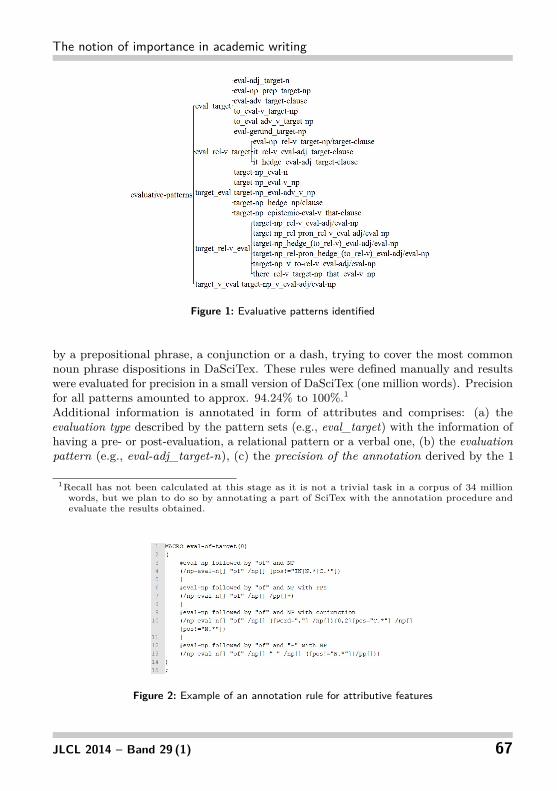
The notion of importance in academic writing
Figure 1: Evaluative patterns identified
by a prepositional phrase, a conjunction or a dash, trying to cover the most commonnoun phrase dispositions in DaSciTex. These rules were defined manually and resultswere evaluated for precision in a small version of DaSciTex (one million words). Precisionfor all patterns amounted to approx. 94.24% to 100%.1Additional information is annotated in form of attributes and comprises: (a) theevaluation type described by the pattern sets (e.g., eval_target) with the information ofhaving a pre- or post-evaluation, a relational pattern or a verbal one, (b) the evaluationpattern (e.g., eval-adj_target-n), (c) the precision of the annotation derived by the 1
1Recall has not been calculated at this stage as it is not a trivial task in a corpus of 34 millionwords, but we plan to do so by annotating a part of SciTex with the annotation procedure andevaluate the results obtained.
Figure 2: Example of an annotation rule for attributive features
JLCL 2014 – Band 29 (1) 67
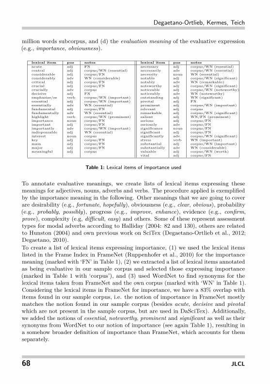
Degaetano-Ortlieb, Kermes, Teich
million words subcorpus, and (d) the evaluation meaning of the evaluative expression(e.g., importance, obviousness).
lexical item pos notes lexical item pos notesacute adj FN necessary adj corpus/WN (essential)central adj corpus/WN (essential) necessarily adv corpus/WN (essential)considerable adj corpus/FN necessity noun WN (essential)considerably adv WN (considerable) notable adj corpus/WN (significant)critical adj corpus/FN notably adv WN (remarkable)crucial adj corpus/FN noteworthy adj corpus/WN (significant)crucially adv corpus noticeable adj corpus/WN (noteworthy)decisive adj FN noticeably adv WN (noteworthy)emphasize/se verb corpus/WN (important) outstanding adj WN (significant)essential adj corpus/WN (important) pivotal adj FNessentially adv WN (essential) prominent adj corpus/WN (important)fundamental adj corpus/FN relevant adj corpusfundamentally adv WN (essential) remarkable adj corpus/WN (significant)highlight verb corpus/WN (prominent) salient adj WN/FN (prominent)importance noun corpus/FN serious adj corpus/FNimportant adj corpus/FN seriously adv corpus/FNimportantly adv corpus/WN (important) significance noun corpus/FNindispensable adj WN (essential) significant adj corpus/FNinterest noun corpus significantly adv corpus/WN (significant)key adj corpus/FN stress verb WN (important)main adj corpus/FN substantial adj corpus/WN (important)major adj corpus/FN substantially adv WN (considerable)meaningful adj corpus valuable adj corpus/WN (worth)
vital adj corpus/FN
Table 1: Lexical items of importance used
To annotate evaluative meanings, we create lists of lexical items expressing thesemeanings for adjectives, nouns, adverbs and verbs. The procedure applied is exemplifiedby the importance meaning in the following. Other meanings that we are going to coverare desirability (e.g., fortunate, hopefully), obviousness (e.g., clear, obvious), probability(e.g., probably, possibly), progress (e.g., improve, enhance), evidence (e.g., confirm,prove), complexity (e.g, difficult, easy) and others. Some of these represent assessmenttypes for modal adverbs according to Halliday (2004: 82 and 130), others are relatedto Hunston (2004) and own previous work on SciTex (Degaetano-Ortlieb et al., 2012;Degaetano, 2010).To create a list of lexical items expressing importance, (1) we used the lexical itemslisted in the Frame Index in FrameNet (Ruppenhofer et al., 2010) for the importancemeaning (marked with ‘FN’ in Table 1), (2) we extracted a list of lexical items annotatedas being evaluative in our sample corpus and selected those expressing importance(marked in Table 1 with ‘corpus’), and (3) used WordNet to find synonyms for thelexical items taken from FrameNet and the own corpus (marked with ‘WN’ in Table 1).Considering the lexical items in FrameNet for importance, we have a 83% overlap withitems found in our sample corpus, i.e. the notion of importance in FrameNet mostlymatches the notion found in our sample corpus (besides acute, decisive and pivotalwhich are not present in the sample corpus, but are used in DaSciTex). Additionally,we added the notions of essential, noteworthy, prominent and significant as well as theirsynonyms from WordNet to our notion of importance (see again Table 1), resulting ina somehow broader definition of importance than FrameNet, which accounts for themseparately.
68 JLCL

The notion of importance in academic writing
Figure 3: Queries used to extract targets
Figure 4: Targets extracted from the eval-adj_target-n pattern
2.4 Extraction of distributional information and targets
Having the patterns and the attributes annotated, we can extract distributional in-formation, i.e. we can, for example, look at how the patterns are distributed acrossdisciplines or how the meaning of importance is used across disciplines and documentsections. The query in Figure 3 line 1, for example, is used to extract instances ofthe meaning of importance. Distributional information across academic disciplines(text_ad) is extracted with the command in line 2. Moreover, we can extract targetsfrom the annotated structures. Depending on where the target is positioned within theevaluative pattern, the complexity of the extraction can vary. For the eval-adj_target-npattern, for example, target extraction is quite simple as the target is located at the endof the annotated pattern. The command for the extraction is shown in Figure 3 line 3.The command in line 4 is executed to extract the targets used in the pattern as well astheir frequencies (see Figure 4). For the relational pattern eval-np_rel-V_target-np theextraction is a bit more complex as the target might be located in the middle of thepattern (see Example (5) above where the target is area A1 ). Here, CQP allows for themarking of specific positions for extraction with the anchor @. Line 5 in Figure 3 showsthe extraction of a nominal target marked by the anchor. The command in line 6 isthen executed to extract the targets and their frequencies.
JLCL 2014 – Band 29 (1) 69

Degaetano-Ortlieb, Kermes, Teich
pattern type pattern eval imp freq eval imp %
eval_target
eval-adj_target-n 13567 64.33eval-np_prep_target_np 863 4.10eval-adv_target-clause 360 1.71eval-v_target-np 252 1.19
eval_rel-v_targetit_rel-v_eval-adj_target-clause 1354 6.47eval-np_rel-v_target-np/clause 1043 4.95ex-there_rel-v_eval-adj/np_target-np 408 1.93
target_evaltarget-n_eval-adv_v_np 295 1.40target_np_eval-n_np 242 1.14target_np_eval-n 88 0.42
target_rel-v_eval target-np_rel-v_eval-adj/np 1504 7.13target-np_v_to_be_eval-np 106 0.50
target_v_eval target-np_v_eval-adv/np 128 4.74
Table 2: Evaluation type and patterns for importance in DaSciTex
3 Analysis: The notion of importance in academic writing
In order to obtain evidence of the attribution of importance in the SciTex corpus, wepose the following questions:
• Which are the linguistic properties of expressions of importance, i.e. whichlexico-grammatical patterns are used?
• Which are the most evaluative sections in a research article and which sectionsexpress more evaluations of importance?
• Are there differences in the use of importance across disciplines and documentsections?
• Which targets are evaluated as being important?
First, we want to know which linguistic properties are used to express importancewithin DaSciTex. This information is obtained by the procedures explained in Section2.4. Table 2 shows that the eval-adj_target-n pattern is the most frequent patternwith 64.33% (realized by expressions as shown in Example (1)). The second mostfrequent pattern is a relational one, target-np_rel-v_eval-adj/np (see Example (7) for arealization), which amounts to approx. 7%. Four other patterns follow: the impersonalit construction with 6.47% (see Example (6)), the relational construction eval-np_rel-v_target-np/clause with 4.95% (see Example (5)), the verbal construction target-np_v_eval-adv/np with 4.74% (see Example (9)), and the prepositional constructionwith 4.10% (such as the importance of linear problem kernels). The other patterns,occur all less than 2.00%. In terms of linguistic properties, the importance meaningis mostly propagated by pre-evaluative structures (84.68% pre-evaluative vs. 15.32%post-evaluative), where the evaluative expression precedes the target.Second, we look at how much evaluation is expressed by the patterns analyzed
and how much of it realizes the meaning of importance across the four documentsections marked in SciTex (Abstract, Introduction, Main and Conclusion). Consideringevaluation overall, we can see that the Introduction and the Conclusion are the mostevaluative sections (both showing approx. 11,300 expressions of evaluation per 1M),
70 JLCL

The notion of importance in academic writing
section section size eval. freq eval. per 1MIntroduction 2150390 24343 11320.27Conclusion 517205 5849 11308.86Abstract 1501711 15765 10498.03Main 11196303 85421 7629.39
Table 3: Evaluation across all document sections in DaSciTex
section eval-imp freq eval-imp per 1MIntroduction 4362 2028.47Abstract 2567 1709.38Conclusion 886 1674.38Main 13459 1202.09
Table 4: Evaluation of importance across document sections in DaSciTex
which is in line with observations made by (Nwogu, 1997), (Hood, 2005) and others.What follows is the Abstract (approx. 10,500) and the Main section (approx. 7600),the latter showing much less evaluation than the other sections (see Table 3).Considering the meaning of importance, the amount in SciTex is of approx. 16%
(131378 occurrences overall of which 21254 are of importance) and the section in whichimportance is mostly used is the Introduction section with approx. 2000 importanceexpressions per 1M (see Table 4). The Abstract and Conclusion sections follow (bothapprox. 1700) as well as the Main part of research articles with the least amountof importance (approx. 1200). Thus, in comparison to all occurrences of evaluationannotated by our approach, the importance meaning occurs mostly at the beginning ofresearch articles (Introduction and Abstract). Additionally, the Abstract shows almostan equal amount of evaluation of importance as the Conclusion, even though it hasless evaluation overall. Comparing the use of evaluation and evaluations of importancein the Introduction and Conclusion sections by chi-square test, we obtain a p-valueof 1.905e-06, i.e. the importance meaning is significantly more often used within theIntroduction section in DaSciTex.Third, we analyze the use of importance across academic disciplines and document
sections. Figure 5 shows that computer science (A) makes the least use of the importancemeaning, linguistics (C1), instead, uses it most frequently and computational linguistics(B1) is somewhere in between. Considering biology (C2) and bioinformatics (B2), theyuse importance quite similarly in amount. For the engineering disciplines, the newlyemerged disciplines, digital construction (B3) and microelectronics (B4), make more useof importance than their seed disciplines, mechanical engineering (C3) and electricalengineering (C4). Considering the distribution across sections for each discipline (seeFigure 6), computer science (A) uses importance most frequently in the Abstractand Introduction and less frequently in the Main part and Conclusion section. Thecomparison of computational linguistics (B1) and linguistics (C1) by chi-square showssignificant differences (p-value of 7.862e-11) due to a higher use of importance in theAbstract for computational linguistics (B1). In comparison to the other disciplines,bioinformatics (B2) and biology (C2) use importance evaluations more frequently withinthe Conclusion section. The engineering disciplines are relatively similar in their use of
JLCL 2014 – Band 29 (1) 71

Degaetano-Ortlieb, Kermes, Teich
Figure 5: Importance across academic disciplines in DaSciTex
Figure 6: Importance across academic disciplines by document sections in DaSciTex
the importance meaning across sections in comparison to the other disciplines.Fourth, we inspect which targets are evaluated with importance across the SciTex
disciplines. As previously mentioned, targets might be realized as nominal phrasesor clauses (e.g., that-clauses). Here, we focus on nominal targets used with the twomost frequent patterns that evaluate a nominal target (eval-adj_target-n and target-np_rel-v_eval-adj/np; see again Table 2). Considering the top 10 to 20 targets acrossdisciplines (see Table 5 for five disciplines), the following observations can be made:(1) we observe domain-specific variation across disciplines (e.g., A-CompSci: function,variable; B1-CompLing: word, document; B2-BioInf: gene, residue), (2) some targetsare shared across disciplines being more general in nature (e.g., difference and role in
72 JLCL

The notion of importance in academic writing
A-CompSci B1-CompLing C1-Ling B2-BioInf C2-Biotarget per 1M target per 1M target per 1M target per 1M target per 1Mresult 52.53 difference 32.00 difference 38.88 gene 53.08 role 90.77problem 12.24 word 25.48 role 33.78 difference 40.17 difference 39.68property 12.24 information 21.92 factor 29.32 role 28.69 factor 22.32idea 11.45 feature 17.78 effect 29.32 feature 27.26 protein 16.86role 8.29 role 17.78 property 24.86 residue 22.24 gene 16.37application 6.71 document 17.18 question 22.95 improvement 19.37 component 15.38question 6.71 problem 16.59 point 17.85 information 18.65 effect 12.90difference 6.32 component 15.41 feature 16.57 problem 15.06 increase 12.90improvement 6.32 issue 14.81 aspect 14.66 issue 13.63 similarity 12.40amount 5.92 point 14.81 issue 14.02 change 12.91 feature 10.91variable 5.53 part 14.22 part 13.39 result 12.19 region 10.42contribution 5.53 improvement 13.63 claim 10.20 component 12.19 change 9.92observation 5.13 question 13.04 discussion 10.20 step 11.48 band 9.42function 4.74 factor 12.44 argument 9.56 number 10.76 amount 8.93packet 4.74 advantage 11.85 number 8.92 part 10.76 step 7.94class 4.34 idea 10.67 way 8.92 pathway 10.76 source 7.94step 4.34 type 10.07 position 8.29 cluster 9.32 function 7.44part 3.95 context 10.07 problem 8.29 idea 9.32 level 7.44point 3.55 property 9.48 constraint 8.29 aspect 8.61 regulator 6.45way 3.16 contribution 8.89 exception 7.65 effect 7.89 decrease 6.45
Table 5: Targets evaluated with importance across five disciplines
the top 10 and improvement, point, problem and question in the top 20).
Figure 7: Domain-specific targets of four disciplines across document sections in DaSciTex
If we look at the domain-specific targets across sections evaluated with importance,we observe that they occur most often either in the Introduction or the Abstract (seeFigure 7). According to previous studies on SciTex (Degaetano-Ortlieb et al., 2013),these targets mostly form keywords in the specific discipline, which indicates thatnominal targets evaluated by importance patterns in most disciplines seem to be topicindicators. Note that this does not mean that they are absent from the Conclusion, theycan be evaluated with other meanings (e.g., application with complex) or the targetschange into hyponyms becoming more specific (e.g., in the case of specific genes).
JLCL 2014 – Band 29 (1) 73

Degaetano-Ortlieb, Kermes, Teich
Figure 8: General targets across document sections in DaSciTex
The more general targets shared across disciplines, instead, show some individualtendencies (see Figure 8). The targets difference and point are distributed relativelyevenly across the sections; problem, question and role, instead, are most frequently usedwithin the Introduction, and improvement is most frequently used in the Conclusionbut also in the Abstract. What these general targets have in common is that they relateto a more specific target. In the case of an improvement, the noun itself bears also anevaluation that is attributed to a target, as in Example (10) where the actual targetis combinatorial algorithms. When we consider question, which is most often used inthe Introduction (similarly to problem and role), it relates mostly to research questionsauthors of research articles pose and emphasize to be important for their study (seeExample (11) and (12)). The general target point, which is quite evenly distributedacross sections (similarly to difference), makes this even more clear, as point itself issomehow an ‘empty’ target. The actual target of the evaluation is what follows therelational verb, which is either a clause or a nominal phrase (see Example (13) and(14), respectively).Another general target used similarly to point mostly in a relational construction isrole. More than 70% (319 out of 446) of role are used within the fixed expression toplay an important role, even though the adjective might vary. In this case, the actualtarget precedes the importance expression (see Example (15)). Thus, role has a morestandardized structure than point which shows more variation.
(10) From this study we conclude that [target−np the combinatorial algorithms] [. . .][v provide] [eval−np significant improvement].
(11) [eval−np Our second major research question] [rel−v is] as follows: [target−np...].
74 JLCL

The notion of importance in academic writing
(12) [eval−np The most crucial question], in our view, [rel−v is] [target−clause whether atemplate-based NLG system can ...].
(13) [eval−np The main point][rel−v is] [target−clause not to dwell on the shortcomings ofthe individual systems, but to ...].
(14) [eval−np One key point in interoperability] [rel−v is] [target−np enterprise modeling].
(15) Observe that [target−np the meaning of the term Ni ( m(j ) = i ) in G3 ] [v plays][eval−np an important role in the algorithm].
If we consider the distribution of role used with importance across disciplines, it ismost frequently used in biology (C2) with 90.77 per 1M and least often in computerscience (A) with 8 per 1M. However, considering how often the fixed expression playan imp-ADJ role is used, computer science (A) uses it most frequently (approx. 81%),while biology (C2) uses it less frequently (approx. 64%). Thus, biology (C2) makes amore varied use of role+importance than computer science (A).
In summary, we can say that academic disciplines (a) differ in the amount of evalua-tions of importance, (b) use different amounts of importance across document sections,and (c) show lexico-grammatical variation in terms of evaluative attribution structuresand evaluated targets.
4 Conclusion and Envoi
We have presented a methodology to approach the detection of evaluative expressionsand targets evaluated on a semi-automatic basis. The manual annotation led the wayto formulate rules for the automatic detection of evaluative expressions and targets.Having the corpus annotated with evaluation patterns and meanings enables furtherinvestigations.In our case, we have focused on the notion of importance in academic research articles.In linguistic terms, we have seen that only particular lexical items and structuresare used to express importance. Considering document sections, Introduction andConclusion are the most evaluative sections, yet the importance meaning is mostlyexpressed at the beginning of research articles. In terms of nominal targets, we have seenthat some general targets are shared across disciplines in SciTex and that they functionalmost as a placeholder. Nominal domain-specific targets instead are evaluated withimportance mostly in the Introduction and Abstract. Thus, we have gained knowledgeon how importance is expressed, where it lies and what it evaluates. Furthermore, wehave seen how the use of evaluative expressions might vary according to the situationalcontext, i.e. academic disciplines.In future work, we aim to investigate more closely full nominal targets as well as clausaltargets across sections and disciplines and to annotate them into the corpus as well ascover other evaluative meanings.Knowledge on evaluative patterns may also improve approaches in sentiment analysis,especially the classification approach in which extraction pattern learning algorithms
JLCL 2014 – Band 29 (1) 75
Degaetano-Ortlieb, Kermes, Teich
may profit from additional input.Knowledge about the contextual configuration of evaluative expressions may providefurther useful information. Considering academic writing, different disciplines makeuse of particular conventions of linguistic feature sets used in that specific situationalcontext. Knowledge on features involved in the formation of these conventions canbe extremely valuable in automatic text classification approaches (Teich et al., 2013;Whitelaw and Argamon, 2004). Additionally, the methodology can be adapted for othergenres to give similar insights.
References
Biber, D., Johansson, S., and Leech, G. (1999). Longman Grammar of Spoken and WrittenEnglish. Longman, Harlow.
CWB (2010). The IMS Open Corpus Workbench. http://www.cwb.sourceforge.net.
Degaetano, S. (2010). Evaluation in Academic Research Articles across Scientific Disciplines.Master’s thesis, Technische Universität Darmstadt.
Degaetano-Ortlieb, S., Hannah, K., Lapshinova-Koltunski, E., and Elke, T. (2013). SciTex – adiachronic corpus for analyzing the development of scientific registers. In Bennett, P., Durrell,M., Scheible, S., and Whitt, R. J., editors, New Methods in Historical Corpus Linguistics,Corpus Linguistics and Interdisciplinary Perspectives on Language (CLIP), Vol. 3. Narr,Tübingen.
Degaetano-Ortlieb, S., Teich, E., and Lapshinova-Koltunski, E. (2012). Domain-specificvariation of sentiment expressions: exploring a model of analysis for academic writing. In 1stWorkshop on Practice and Theory of Opinion Mining and Sentiment Analysis (PATHOS)at Konvens2012, Vienna.
Evert, S. (2005). The CQP Query Language Tutorial. IMS Stuttgart. CWB version 2.2.b90.
Hood, S. (2005). Managing attitude in undergraduate academic writing: a focus on theintroductions to research reports. In Ravelli, L. J. and Ellis, R. A., editors, AnalysingAcademic Writing. Contextualized Frameworks. Continuum, London & New York.
Hundt, M., Sand, A., and Siemund, R. (1999). Manual of Information to Accompany TheFreiburg – LOB Corpus of British English (‘FLOB’). Freiburg: Department of English,Albert-Ludwigs-Universität Freiburg.
Hunston, S. (2004). Counting the uncountable: problems of identifying evaluation in a textand in a corpus. In Corpora and Discourse, pages 157–188. Peter Lang.
Hunston, S. (2011). Corpus approaches to evaluation: phraseology and evaluative language.Taylor & Francis, London.
Hunston, S. and Francis, G. (2000). Pattern Grammar: A Corpus-driven Approach to theLexical Grammar of English. Studies in Corpus Linguistics. John Benjamins Publishing,Amsterdam/Philadelphia.
Hyland, K. (2005). Stance and engagement: a model of interaction in academic discourse.Discourse Studies, 7(2):173–192.
76 JLCL
The notion of importance in academic writing
Kermes, H. (2003). Off-line (and On-line) Text Analysis for Computational Lexicography. PhDthesis, Universität Stuttgart.
Kučera, H. and Francis, W. N. (1967). Computational Analysis of Present-Day AmericanEnglish. Brown University Press, Providence, RI.
Martin, J. R. and White, P. R. (2005). The Language of Evaluation, Appraisal in English.Palgrave Macmillan, London & New York.
Nwogu, K. N. (1997). The medical research paper: Structure and functions. English for SpecificPurposes, 16(2):119–138.
O’Donnell, M. (2008). The UAM CorpusTool: Software for corpus annotation and exploration.In Proceedings of the XXVI Congreso de AESLA, Almeria, Spain.
Ruppenhofer, J., Ellsworth, M., Petruck, M. R. L., Johnson, C. R., and Scheffczyk, J. (2010).Framenet II: Extended theory and practice. Technical report, ICSI.
Schmid, H. (1994). Probabilistic Part-of-Speech Tagging Using Decision Trees. In InternationalConference on New Methods in Language Processing, pages 44–49, Manchester, UK.
Swales, J. M. (1990). Genre Analysis. English in academic and research settings. CambridgeUniversity Press, Cambridge.
Teich, E., Degaetano-Ortlieb, S., Kermes, H., and Lapshinova-Koltunski, E. (2013). Scientificregisters and disciplinary diversification: a comparable corpus approach. In Proceedings of6th Workshop on Building and Using Comparable Corpora (BUCC), Sofia, Bulgaria.
Teich, E. and Fankhauser, P. (2010). Exploring a corpus of scientific texts using data mining. InGries, S., Wulff, S., and Davies, M., editors, Corpus-linguistic applications: Current studies,new directions, pages 233–247. Rodopi, Amsterdam & New York.
Whitelaw, C. and Argamon, S. (2004). Systemic functional features in stylistic text classification.In AAAI Fall Symposium Series, Washington D.C., USA.
Wilson, T. A. (2008). Fine-grained Subjectivity and Sentiment Analysis: Recognizing theIntensity, Polarity, and Attitudes of Private States. PhD thesis, University of Pittsburgh.
JLCL 2014 – Band 29 (1) 77

JLCL 2014 – Band 29 (1) – 79-94
Yuqiao Gu, Fabio Celli, Josef Steinberger, Andrew James Anderson, Massimo Poesio, Carlo Strapparava and Brian Murphy
Using Brain Data for Sentiment Analysis
Abstract We present the results of exploratory experiments using lexical valence extracted from brain
using electroencephalography (EEG) for sentiment analysis. We selected 78 English words
(36 for training and 42 for testing), presented as stimuli to 3 English native speakers. EEG
signals were recorded from the subjects while they performed a mental imaging task for
each word stimulus. Wavelet decomposition was employed to extract EEG features from the
time-frequency domain. The extracted features were used as inputs to a sparse multinomial
logistic regression (SMLR) classifier for valence classification, after univariate ANOVA
feature selection. After mapping EEG signals to sentiment valences, we exploited the lexical
polarity extracted from brain data for the prediction of the valence of 12 sentences taken
from the SemEval-2007 shared task, and compared it against existing lexical resources.
1 Introduction and related work
Sentiment analysis—automatically recognizing the emotions conveyed by a text, and in
particular distinguishing positive from negative valence—has become one of the most popu-
lar research areas in computational linguistics (Pang & Lee, 2008; Liu, 2012) both because
of the interest of the field in the interplay between emotion and cognitive abilities, and be-
cause of its obvious applications (e.g., companies could analyze social networks to deter-
mine customer response to their products). Such research however requires collecting judg-
ments about the valence of sentences and possibly lexical items, and simply asking subjects
often results in low inter-annotator agreement levels (Arnstein & Poesio 2008; Craggs &
McGee Wood, 2004; Esuli & Sebastiani 2006). But this difference between subjective
judgments may be caused by strategic effects rather than unconscious processes as measured
with neuroimaging techniques. And indeed, Crosson et al. (1999, 2002) and Cato et al.
(2004) demonstrated that it is possible to discriminate positive and negative words from
neutral words on the basis of the blood-oxygen-level dependent (BOLD) signal collected
through functional magnetic resonance imaging (fMRI) scans. Using magnetoencephalo-
graphy (MEG) recording techniques, Hirata et al., 2007 found that negative and positive
words can be distinguished by event-related desynchronizations (ERDs). These results sug-
gest that valence information might be best collected without asking the subjects directly. In
the future it may be possible to use neuroimaging to benefit sentiment analysis e.g. by tap-
ping into subconscious valence representations which could reduce annotator rating time; or
provide us more nuanced ways to measure valence. The long-term aim of our project is to
assess the feasibility of using for sentiment analysis valence information derived from the
brain.
The focus of the preliminary investigation discussed in this paper was primarily practical:
to address one of the issues that have to be faced in order to achieve the ultimate goal. The
problem is that the cost of collecting valence information through fMRI or MEG would be
prohibitive at present. On the other hand, EEG is a very inexpensive and widespread tech-
nology. Taking advantage of its high temporal resolution, in recent years EEG and event-

JLCL
Gu et al.
80
related potentials (ERPs) was intensively used in psycholinguistics, e.g., for the investiga-
tion of processing mechanisms of semantic categories (Pulvermüller et al., 1999; Kiefer
2001; Paz-Caballero et al., 2006; Proverbio et al., 2007; Hoenig, et al., 2008; Adorni &
Proverbio, 2009; Fuggetta, et al., 2009; Renoult & Debruille, 2010; Renoult et al., 2012).
Hagoort et al. (2004) studied the integration of word meaning and world knowledge with
EEG, ERP and fMRI while subjects read sentences. In some sentences the critical words
make the sentences a correct or false semantic interpretation and in other sentences the criti-
cal words make the sentence a correct or false world knowledge interpretation. Using EEG
and ERP, Delong et al. (2005) found that individuals can use linguistic input to pre-activate
representations of upcoming words in advance of their appearance. Using event-related EEG
and multivariate pattern analysis, Simanova et al., 2010 studied the conceptual representa-
tion and classification of object categories in different modalities. In other work, we have
used EEG and machine learning to decode the semantic categories of animals vs tools in
younger and elderly subjects during a covert image naming task (Murphy et al., 2011; Gu et
al., 2013). In this work, we apply this approach to the decoding of the emotional valence of
written words, and propose a novel paradigm for using such decoding techniques for senti-
ment analysis.
The structure of the paper is as follows. First of all we describe the paradigm in general
terms. Next we discuss how we used a linguistically controlled data set of word stimuli to
elicit EEG data about valence and to train a within-subjects valence classifier which was
then used to assign valence to words in the test set. Finally, we discuss preliminary experi-
ments using this valence for sentiment analysis.
2 Methodology
A number of issues need to be tackled in order to use brain data to determine the valence of
words. The first problem, already mentioned, is that fMRI as used by Cato et al is very ex-
pensive (the costs are in the order of €500 per hour) and requires substantial medical infra-
structure. As already mentioned, our solution to this problem was to use EEG, which costs
substantially less and is becoming a standard facility also in Computer Science and Psychol-
ogy labs.
But even using EEG, it is not possible to get the valence of each word directly from sub-
jects. Generally at least 5-6 presentations of a stimulus (word) to each subject are needed to
get a stable representation of the signal for that stimulus and that subject. At a few seconds
per stimulus, at most 80 stimuli can be presented to a subject in one hour—the duration of
time after which the subject’s attention generally is lost. This makes it time-consuming to
measure brain activity for even the relatively small number of words in a standard corpus.
Creating an EEG-based sentiment dictionary would require multiple sessions for multiple
participants. In these experiments we used a test subset of the corpus created for the Senti-
ment Analysis at SemEval-2007 (Strapparava & Mihalcea, 2007) as test data. The corpus
consists of about 250 examples of news titles in the trial set and about 1000 in the test set.
News titles have been extracted from news web sites (such as Google news, CNN) and/or
newspapers. Each example is labeled with emotions (anger, disgust, fear, joy, sadness, sur-
prise) and polarity (positive/negative). The test data was independently labeled by six anno-

81 JLCL 2014 – Band 29 (1)
Using Brain Data for Sentiment Analysis
tators. Annotation was performed using a web-based interface that displayed one headline at
a time, together with a slide bar for valence assignment. The interval for the valence annota-
tions was set from -100 to 100, where 0 represents a neutral headline, -100 represents a
highly negative headline and 100 corresponds to a highly positive headline. We selected
only positive or negative sentences, not neutral ones. The inter-annotator agreement for the
sentiment polarity is 0.78 (Pearson's correlation).
In order to address the problem mentioned above we proceeded as follows. First of all we
specified a training dataset consisting of 36 stimuli—12 positive, 12 negative, and 12 neu-
tral—from behavioral norms (Vinson & Vigliocco 2008; Coltheart, 1981) on whose valence
there is substantial agreement among a large number of subjects. Every subject sees each
stimuli 5 times. The signal collected from these stimuli is used to train a per-subject valence
classifier that is then used to assign a predicted valence to 42 stimuli from the testing dataset
(words occurring in a subset of the SemEval test set). The predicted word valences are then
fed into a classifier for predicting the overall valence of 12 selected sentences. Our working
hypothesis is that the positive, neutral and negative valence of words may be processed by
different neural mechanisms and the valence information can be reflected by and extracted
from the EEG data. The trained classifier maps the EEG feature space into the negative,
neutral and positive valences. Therefore the trained classifier should be able to predict the
valence of any test word. Figure 1 sketches out the working procedure described here.
Figure 1: Schematic procedure using brain data for sentiment analysis.

JLCL
Gu et al.
82
Last but not least, there is the problem of achieving a good performance on determining
predicted valence. The performance of EEG at lexical information (Murphy et al., 2011) is
typically not comparable to that obtained using fMRI (Mitchell et al., 2008; Pereira et al.,
2009). In particular with EEG it is typically more difficult to achieve good inter-subject
classification. This can be attributed to the following: 1) the poor spatial resolution of EEG
signal; 2) differences in emotional experience between participants. For this reason at pre-
sent we collect both training and testing data from the same subject.
3 Using machine learning to decode and predict the valence of English
words from EEG data
In this Section we discuss how we used EEG to decode the emotional valence of English
words.
3.1 EEG experiment and data preprocessing
Materials. Previous work (Kousta et al., 2009; Kousta et al., 2011) suggests that there are
likely to be differences with regards to extracting valence between abstract and concrete
words. We used therefore a dataset classified according to two dimensions: abstract vs. con-
crete, or according to their emotional valence (negative, neutral and positive). 36 words
were manually selected to vary appropriately in concreteness and valence ratings between
the 6 experimental categories and to be otherwise matched in terms of a comprehensive list
of linguistic parameters that could serve as confounds. To validate the final set of words, 2-
way analysis of variance was undertaken to verify that the experimental groups did not sig-
nificantly differ in any undesirable way. Results are shown in table 1, where V denotes the
main effect was valence category, C denotes the main effect was concreteness category and
C×V is the interaction.
Linguistic parameters V C C×V
F(1,30) p F(2,30) p F(2,30) p
Valence 0.02 0.88 201.26 0 0.89 0.42
Concreteness 266.7 0 0.06 0.93 0.88 0.43
Number of letters 0 1 0 1 0 1
Imageability 84.18 0 0.24 0.79 0.45 0.64
Arousal 0.16 0.7 2.9 0.07 1.35 0.27
Age of acquisition 2.6 0.12 0.25 0.78 0.6 0.56
Familiarity 0.41 0.53 0.58 0.56 1.12 0.34
Log frequency 0 0.99 0.71 0.5 1.22 0.31
Number of orthographic neighbours 0.52 0.47 0.06 0.94 0.15 0.86
Bigram frequency 0.95 0.37 0.1 0.9 0.25 0.78
Number of morphemes 1 0.33 1 0.38 1 0.38
Table 1: Results of 2-way analysis of variance on the training set.
For the test set, we chose 12 sentences from the dataset provided in the SemEval-2007
Sentiment Analysis Task 14 (Strapparava & Mihalcea, 2007) and chose the 42 most frequent

83 JLCL 2014 – Band 29 (1)
Using Brain Data for Sentiment Analysis
non-stopword nouns. The sentences were chosen in order to have a balance between posi-
tive, neutral and negative polarities, as well as between concrete and abstract words. The
stimuli in the training set and test set are listed in Table 2. The 12 sentences are listed in
Table 3.
Participants. One PhD student and two postdoctoral fellows at the University of Trento
took part in the study, all native speakers of English. One participant was male and two fe-
male (age range 26–37, mean 33). One identified herself as left-handed, and two as right-
handed. All had normal or corrected-to-normal vision. Participants received compensation
of €7 per hour. The studies were conducted under the approval of the ethics committee at the
University of Trento, and participants gave informed consent.
Training set
Abstract
Negative harm, hurt, gloom, deceit, terror, sorrow
Neutral mood, guess, minute, motive,span, trance
Positive cure, ease, peace, reward, warmth, virtue
Concrete
Negative jail, scar, blood, corpse, cancer, poison
Neutral mule, cart, waist, marble, barrel, cement
Positive silk, cash, heart, palace, cherry, silver
Test set
Abstract
save , sick, switch, fetal, loss, swallow, technology, crash, plan, warn-ing, copyright, reject, claim, health, university, offer, support, rabies, suspect, debate, miracle, hail, release, marathon
Concrete Squirrel, boy, park, school, scientist, cocoa, suburb, riot, committee Vaccine, helicopter, river, dolphin, pill, parents, gene
Table 2: Stimuli in the training and test set.
Number Sentence Polarity
1 Squirrel jumps boy in park; rabies suspected -71 2 University offers support to New Orleans school +60 3 Beyonce copyright claim rejected -7 4 Scientists tout cocoa's health benefits +72 5 Riot warning for France suburbs -64 6 Committee debates cancer vaccine plan +2 7 Die As US Helicopter Crashes in Iraq -93 8 Technology may save India's river dolphins +67 9 Poison Pill to Swallow: Hawks Hurting After Loss to Vikes -35 10 Rescued boys parents hail 'miracle' +71 11 Sick hearts switch on a fetal gene -12 12 Marathon winner released from hospital +70
Table 3: Test sentences. The words extracted in the test set are highlighted by italic format
Experimental paradigm. Participants saw written words on the screen, repeated 5 times
in random order, and are asked to imagine situations exemplifying the words. Once the situ-
ation came to mind they responded with a button press. Words were presented until button
press, or to a timeout of 5s. Fixations and blanks added 3s per trial. Participants sat in a re-

JLCL
Gu et al.
84
laxed upright position 60 cm from a computer monitor in reduced lighting conditions. The
task duration was split into five blocks and participants were given the choice to pause be-
tween each. Each trial began with the presentation of a fixation cross for 0.5 s, followed by
the stimulus word, a further fixation cross for 0.5 s and a blank screen for 2 s. Participants
were asked to keep still during the task, and to avoid eye-movements and facial muscle ac-
tivity in particular, except during the 2s blank period.
EEG recording and data preprocessing. The experiment was conducted at the CI-
MeC/DiSCoF laboratories at University of Trento, using a 64-electrode Brain Vision Brain-
Amp system, recording at 500 Hz. A wide-coverage montage based on the 10–20 system
was used, with a single right earlobe reference, and ground at location AFz. Electrode im-
pedances were generally kept below 10 kOhms. However, sessions including electrodes that
exceeded this limit were still included in subsequent analysis, as the techniques used proved
robust to such noise. Data preprocessing was conducted using the EEGLAB package (De-
lorme & Makeig, 2004). The data was band-pass filtered at 1–50 Hz to remove slow drifts in
the signal and high-frequency noise, and then down-sampled to 125 Hz. An ICA analysis
was next applied using the EEGLAB implementation of the Infomax algorithm (Makeig et
al., 1996). Artefactual ICA components were then identified and removed by hand in each
dataset. Eye-artefact components were removed –usually one component for vertical move-
ments including blinks, and another for horizontal movements.
3.2 EEG data analysis and classification
Wavelet Feature extraction and selection. To classify the EEG data, first of all we ex-
tracted data epochs from the preprocessed data in a time window after stimulus onset.
1D multilevel discrete wavelet transform decomposition was employed to extract the de-
composition coefficients of the epoched EEG data in the time-frequency domain. Two
wavelet functions: coif3 and db7, were used. For a given EEG epoch of a given channel,
extracted features were ordered as a list of coefficients arrays in the form [cA_n, cD_n,
cD_n-1, ..., cD2, cD1], where n denotes the level of decomposition. The first element
(cA_n) of the list is an approximation coefficients array and the following elements (cD_n to
cD_1) are details of coefficients arrays. Figure 2 illustrates one EEG epoch of Fpz channel
and the extracted wavelet approximation coefficients array and details of coefficients arrays.
For a given trial, the extracted EEG features are collected in a wavelet coefficients array
whose number of elements equals to the number of channels × the number of coefficients of
a single trial in a single channel.
Usually, the number of the extracted features is huge and the feature array contains many
redundant or irrelevant features for valence classification. Taking the epoch from 0.1 to 1.4
seconds as an example, the number of the extracted EEG features of each trial is 13568 (=
64 × 212, where 64 is the number of channels and 212 the number of extracted wavelet co-
efficients). To shorten classifier training time, improve model interpretability and enhance
model generalization, we employed univariate ANOVA to select the most promising 3000
features with the highest F-scores.
Classification. A SMLR classifier (Krishnapuram et al., 2005) was used in 10, 20 and 30
fold cross-validation analyses. The training dataset was constructed by the wavelet features

85 JLCL 2014 – Band 29 (1)
Using Brain Data for Sentiment Analysis
Figure 2: One EEG epoch of Fpz channel and its 5 level wavelet decomposition coefficients.
corresponding to the trials with stimuli in the training set of the words in Table 2. For a giv-
en category, abstract (negative, neutral, positive) or concrete (negative, neutral, positive), in
the training dataset the total number of samples was 90 (18 words × 5 replicates).
Prediction. The test dataset was constructed by the wavelet features corresponding to
the trials with stimuli in the test set of the words in Table 2. The test dataset contained 18×
5=90 concrete words and 24×5=120 abstract words. The test dataset were used as input to
the trained classifier to predict the valence of the test words by assigning a valence to each
EEG trial with trigger number in the test set.
3.3 Results
In order to get better classification of the emotional valence of English words, we separately
classified the valence of concrete and abstract words.
Training the classifier. To train the classifier, for each subject, we tried different time
epochs and two wavelet functions coif3 and db7. We found a time period from 0.1 to 1.6
seconds after stimulation onset, in which the classification accuracy is higher. The classifi-
cation results of the training words are shown in Table 4. Here we show the best classifica-
tion accuracy for each subject within a time window in the period 0.1 to 1.6 seconds. The

JLCL
Gu et al.
86
chance to classify into three classes is 33.3%. Our classification accuracy is from 43% to
63%, which is well above chance.
For each concrete and abstract category of each dataset we have also calculated mean
classification accuracy over 10 time windows (0.1 or 0.2 to 0.7 + 0.1×n seconds, where n =
0, 1, 2, …, 9). For abstract category, the mean classification accuracy is (43.45±3.62)% for
subject 1, (54.44±3.88)% for subject 2 and (40.00±4.67)% for subject 3. For concrete cate-
gory, the mean classification accuracy is (56.45±3.73)% for subject 1, (52.44±4.81)% for
subject 2 and (51.63±6.09)% for subject 3. This result indicates the mean classification ac-
curacies are also well above chance. Especially the three mean classification accuracies of
the concrete category are greater than 50%. To study the effect of number of selected fea-
tures on the classification accuracy, we reduce the number of selected EEG features. We
found that for the concrete category, using 300 selected features to train the classifier one
can get mean accuracy well above chance. However, for abstract category, in order to get
mean accuracy well above chance we have to use 1000 selected features to train the classifi-
er. Therefore we used 1000 selected features for abstract category and from 300 for concrete
category to train the classifier. Then we calculated mean classification accuracy over 10
time windows. For abstract category, the mean classification accuracy is (41.20±5.71)% for
subject 1, (51.44±4.94)% for subject 2 and (38.49±4.85)% for subject 3. For concrete cate-
gory, the mean classification accuracy is (42.32±4.67)% for subject 1, (42.17±3.41)% for
subject 2 and (48.98±4.03)% for subject 3. This result suggests that the classification accu-
racy decreases with the number of selected features.
We have randomized the trials of the feature array so that the relationship between the ex-
tracted features and the valence label of each trial is randomly matched. We used such ran-
dom features as input to train the classifier (3000 selected features, 20-fold). Then we calcu-
lated the mean classification accuracy over 20 such random EEG for concrete and abstract
classes of each dataset in the same epoch as given in Table 4. For abstract category, the
mean classification accuracy is (42.94±6.86) % for subject 1, (41.51±5.73)% for subject 2
and (37.98±6.77)% for subject 3. For concrete category, the mean classification accuracy is
(42.65±8.61)% for subject 1, (42.34±5.89)% for subject 2 and (41.61±4.88)% for subject 3.
The mean accuracy is between (37.98±6.77)% and (42.94±6.86)%. Considering that this
result is probably caused by the large number of EEG features, we reduce the number of
selected EEG features from 3000 to 1000 for abstract category and from 3000 to 300 for
concrete category to train the classifier by the permuted EEG data from 0.1 to 1.6 seconds
after stimuli onset. Then we calculated the mean classification accuracy over 20 such per-
muted EEG for concrete and abstract classes of each dataset. For abstract category, the mean
classification accuracy is (37.07±5.26)% for subject 1, (40.11±7.99)% for subject 2 and
(36.74±7.08)% for subject 3. For concrete category, the mean classification accuracy is
(33.52±9.36)% for subject 1, (36.5±5.77)% for subject 2 and (37.35±6.22)% for subject 3.
Predicting the valence of test words. For each dataset, the classifier trained by the train-
ing trials with inside 20-fold training/testing partitions of the data was employed to predict
the valence of the words in the test trials. The prediction lists of the abstract and concrete
words from the three subjects were employed for sentiment analysis in the following Sec-
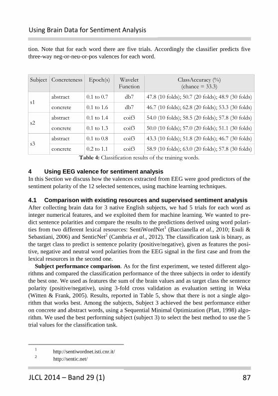
87 JLCL 2014 – Band 29 (1)
Using Brain Data for Sentiment Analysis
tion. Note that for each word there are five trials. Accordingly the classifier predicts five
three-way neg-or-neu-or-pos valences for each word.
Subject Concreteness Epoch(s) Wavelet Function
ClassAccuracy (%) (chance = 33.3)
s1 abstract 0.1 to 0.7 db7 47.8 (10 folds); 50.7 (20 folds); 48.9 (30 folds)
concrete 0.1 to 1.6 db7 46.7 (10 folds); 62.8 (20 folds); 53.3 (30 folds)
s2 abstract 0.1 to 1.4 coif3 54.0 (10 folds); 58.5 (20 folds); 57.8 (30 folds)
concrete 0.1 to 1.3 coif3 50.0 (10 folds); 57.0 (20 folds); 51.1 (30 folds)
s3 abstract 0.1 to 0.8 coif3 43.3 (10 folds); 51.8 (20 folds); 46.7 (30 folds)
concrete 0.2 to 1.1 coif3 58.9 (10 folds); 63.0 (20 folds); 57.8 (30 folds)
Table 4: Classification results of the training words.
4 Using EEG valence for sentiment analysis
In this Section we discuss how the valences extracted from EEG were good predictors of the
sentiment polarity of the 12 selected sentences, using machine learning techniques.
4.1 Comparison with existing resources and supervised sentiment analysis
After collecting brain data for 3 native English subjects, we had 5 trials for each word as
integer numerical features, and we exploited them for machine learning. We wanted to pre-
dict sentence polarities and compare the results to the predictions derived using word polari-
ties from two different lexical resources: SentiWordNet1 (Baccianella et al., 2010; Esuli &
Sebastiani, 2006) and SenticNet2 (Cambria et al., 2012). The classification task is binary, as
the target class to predict is sentence polarity (positive/negative), given as features the posi-
tive, negative and neutral word polarities from the EEG signal in the first case and from the
lexical resources in the second one.
Subject performance comparison. As for the first experiment, we tested different algo-
rithms and compared the classification performance of the three subjects in order to identify
the best one. We used as features the sum of the brain values and as target class the sentence
polarity (positive/negative), using 3-fold cross validation as evaluation setting in Weka
(Witten & Frank, 2005). Results, reported in Table 5, show that there is not a single algo-
rithm that works best. Among the subjects, Subject 3 achieved the best performance either
on concrete and abstract words, using a Sequential Minimal Optimization (Platt, 1998) algo-
rithm. We used the best performing subject (subject 3) to select the best method to use the 5
trial values for the classification task.
1 http://sentiwordnet.isti.cnr.it/
2 http://sentic.net/

JLCL
Gu et al.
88
Feature selection: all trials vs. sum of values. We ran an experiment to test how the dif-
ferent brain outcomes in the 5 trials can be exploited to achieve the best results. In one test
we used all the 5 trials as features, while in the second test we exploited the sum of the val-
ues —which can be +1, -1 and 0— as one feature. As before, we used a 3-fold cross valida-
tion in Weka. The result, computed using SMO and averaged over the three subjects and
over abstact and concrete words, are f1=0.442 using all the values, and f1=0.407 using the
sum of trials.
Comparing brain data and lexical resources. Then we extracted from SentiWordNet
and SenticNet all the values associated to the selected words, leaving a tie if no values were
available. We had 14 ties with SenticNet and no ties with SentiWordNet. SenticNet provides
one polarity value (positive or negative), while SentiWordNet provides one value for the
positive pole and one for the negative one. Polarities from SentiWordNet have been extract-
ed from the first sense; if both positive and negative values were available, we used the dif-
ference between the two.
Data Concreteness Algorithm Precision Recall F1measure
baseline
abstract
zeroRule 0.25 0.5 0.333
s1 SMO 0.349 0.375 0.347
s2 bayes 0.594 0.583 0.571
s3 SMO 0.752 0.708 0.695
senticNet SMO 0.757 0.75 0.748
SentiWN logistic 0.853 0.792 0.782
baseline
concrete
zeroRule 0.309 0.556 0.397
s1 logistic 0.494 0.5 0.495
s2 bayes 0.444 0.444 0.444
s3 SMO 0.797 0.778 0.778
SenticNet logistic 0.728 0.722 0.723
SentiWN SMO 0.477 0.5 0.475
Table 5: Comparison of supervised analysis results obtained by brain data and dictionaries.
Like before, we ran the experiment using 3-fold cross validation in Weka to predict the
polarity of sentences. Results, reported in Table 5, show that lexical resources yield better
classification performances for abstract words, but also that subject 3 achieved the best per-
formance on concrete words. The correlation coefficients are r = 0.648 for subject 3 with
concrete words and r = 0.345 with SentiWordNet on abstract words.
89 JLCL 2014 – Band 29 (1)
Using Brain Data for Sentiment Analysis
4.2 Integrating the valence in a state-of-the-art unsupervised sentiment
analysis system
For the unsupervised scenario we used the sentiment analyser (Steinberger et al., 2011)
developed as part of the Europe Media Monitor (Atkinson & Van der Goot, 2009). The ob-
jective of the analyser is to detect positive or negative opinions expressed towards entities in
the news across different languages and to follow trends over time.
It attaches a sentiment score to all entity mentions, mainly persons and organizations. It
uses a fixed window of 6 terms, which was found to be optimal in the analysis in Balahur et
al., 2010, around the entity mention to look for sentiment terms. The approach also accounts
for contextual valence shifting (negations, diminishers and intensifiers). In their case, the
approach is rather defensive, as it looks for shifters only two terms around each sentiment
term. This way it captures the most common shifters (very good, not good, less good) but
modals or adverbs with larger scope may not be captured. For our purpose the tool was
modified to analyze the whole sentence regardless an entity mention and regardless any
fixed window for sentiment terms.
The approach uses language-specific sentiment dictionaries. Inspired by the positive ef-
fect of introducing two levels of sentiment intensity in Balahur et al., 2010, it uses more
classes. The score of positive terms is 2, negative -2, very positive 4, and very negative -4. If
a polar expression is negated, its polarity score is simply inverted. In the case of term with
higher intensity we lower the intensity. In a similar fashion, diminishers are taken into con-
sideration. The difference is, however, that the score is only reduced rather than shifted to
the other polarity type. Special care has to be taken when shifters are combined: for example
not very good – good carries the score (+2), it is intensified by very (+3) and inverted by
not, however, if we take the same approach as in the case of optimal above, the result is (-2).
The scores of the sentiment terms found in a sentence are summed up and the normalized
score gives the final sentiment of the sentence. The score ranges from -100 to +100, where,
for instance, 100 corresponds to a case with all the terms very positive. The score thus corre-
sponds to the range of SemEval-2007.
Sentiment Dictionaries. We tested the following resources:
WordNet Affect (WNA) (Strapparava & Valitutti, 2004): categories of anger and
disgust were grouped under high negative, fear and sadness were considered nega-
tive, joy was taken as containing positive words and surprise as highly positive.
SentiWordNet (SWN) (Esuli & Sebastiani, 2006): we used the difference between
the positive and negative scores. We mapped the positive scores lower than 0.75
to the positive category, the scores higher than 0.75 to the highly positive set, the
negative scores lower than 0.75 to the negative category and the ones higher than
0.75 to the highly negative set.
MicroWordNet (MWN) (Cerini et al., 2007): the mapping was similar to Senti-
WordNet.
General Inquirer (GI) (Stone et al., 1966): besides other annotations, each English
word is labeled as “positive outlook” or “negative outlook” in GI. Terms taken
from these categories formed one of the first sentiment dictionaries.
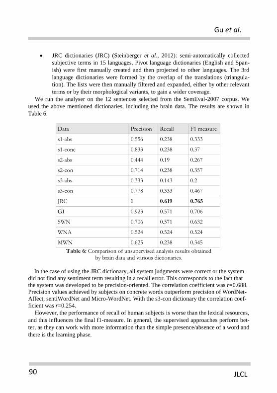
JLCL
Gu et al.
90
JRC dictionaries (JRC) (Steinberger et al., 2012): semi-automatically collected
subjective terms in 15 languages. Pivot language dictionaries (English and Span-
ish) were first manually created and then projected to other languages. The 3rd
language dictionaries were formed by the overlap of the translations (triangula-
tion). The lists were then manually filtered and expanded, either by other relevant
terms or by their morphological variants, to gain a wider coverage.
We run the analyser on the 12 sentences selected from the SemEval-2007 corpus. We
used the above mentioned dictionaries, including the brain data. The results are shown in
Table 6.
Data Precision Recall F1 measure
s1-abs 0.556 0.238 0.333
s1-conc 0.833 0.238 0.37
s2-abs 0.444 0.19 0.267
s2-con 0.714 0.238 0.357
s3-abs 0.333 0.143 0.2
s3-con 0.778 0.333 0.467
JRC 1 0.619 0.765
GI 0.923 0.571 0.706
SWN 0.706 0.571 0.632
WNA 0.524 0.524 0.524
MWN 0.625 0.238 0.345
Table 6: Comparison of unsupervised analysis results obtained by brain data and various dictionaries.
In the case of using the JRC dictionary, all system judgments were correct or the system
did not find any sentiment term resulting in a recall error. This corresponds to the fact that
the system was developed to be precision-oriented. The correlation coefficient was r=0.688.
Precision values achieved by subjects on concrete words outperform precision of WordNet-
Affect, sentiWordNet and Micro-WordNet. With the s3-con dictionary the correlation coef-
ficient was r=0.254.
However, the performance of recall of human subjects is worse than the lexical resources,
and this influences the final f1-measure. In general, the supervised approaches perform bet-
ter, as they can work with more information than the simple presence/absence of a word and
there is the learning phase.

91 JLCL 2014 – Band 29 (1)
Using Brain Data for Sentiment Analysis
5 Conclusions
In this paper we report exploratory experiments testing whether text valence can be reliably
extracted from brain signals using EEG—at present, the only technology that can be ex-
pected to be usable to elicit brain information on a large scale, in particular when the new
generation of low-cost headsets will appear. Our results demonstrated that the emotional
valence information of words can indeed be extracted by wavelet decomposition coefficients
and classified by machine learning with accuracy well above chance.
We also carried out very preliminary experiments using lexical valence extracted from
EEG for sentiment analysis of a small set of sentences from a standard dataset, using both
supervised and unsupervised machine learning techniques. For those sentences at least, the
precision achieved using lexical valence extracted from EEG is close to the one obtained
using standard sentiment dictionaries such as WordNet Affect, senticNet or SentiWordNet.
EEG-based sentiment analysis results are even better when using supervised learning. We
conclude that the paradigm we propose might indeed develop into an alternative technique
for collecting valence.
Our next step will be to test these methods on a larger scale, in three respects. First of all,
we started to use larger datasets of sentences from the sentiment analysis shared task at
SemEval-2013; and to test our methods on Italian as well as English. Second, we started to
also use adjectives, adverbs and verbs as stimuli. Last but not least, we started to investigate
the effect of context on the valence of words such as rude that have a negative valence in
sentences such as You’re being rude but a positive one in sentences such as I found him in
rude health. We intend to study how the valences of emotional words are modified by dif-
ferent contexts and how their emotional categories change with contexts. We are also inter-
ested in investigating how the emotional words and emotional mood exert influence on sen-
tence processing and on the polarity of sentences, as it has been recently found that emo-
tional valence in a word and emotional mood of the participants inducted by film clips im-
pact the syntactic and semantic processing (Chwilla et al., 2011; Martín-Loeches, et al.,
2012). From a methodological perspective, we aim to improve the classification accuracy by
selecting most informative channels and extracting other EEG features such as event-related
potential and the reconstructed wavelet approximation and details of the EEG data.
Acknowledgements
This research was carried out as part of the Deep Relations project, a collaboration
between CIMEC, Expert Systems and Fondazione Bruno Kessler (FBK) funded by the
Provincia di Trento. It was also partly supported by projects: NTIS (Net Technologies for
Information Society), European Center of Excellence, CZ.1.05/1.1.00/02.0090 and
MediaGist. EU’s FP7 People Programme (Marie Curie Actions), no 630786.
References
Adorni, R., Proverbio, A.M. (2009). New insights into name category-related effects: is the Age of
Acquisition a possible factor? Behav Brain Funct 5: 33.
Artstein R., Poesio M.. (2008). Intercoder agreement for Computational Linguistics. In Computational
Linguistics, 34(4): 555—596.
JLCL
Gu et al.
92
Atkinson, M. and Van der Goot, E. (2009). Near Real Time Information Mining in Multilingual News.
In 18th International World Wide Web Conference, WWW.
Baccianella, S., Esuli, A., and Sebastiani, F. (2010). SentiWordNet 3.0: An Enhanced Lexical Resource
for Sentiment Analysis and Opinion Mining. In LREC(10): 2200-2204.
Balahur, A., Steinberger, R., Kabadjov, M., Zavarella, V., Van der Goot, E., Halkia, M., Pouliquen, B.,
and Belyaeva, J. (2010). Sentiment analysis in the news. In Proceedings of the 7th International
Conference on Language Resources and Evaluation, LREC.
Cambria, E., Havasi, C., and Hussain, A. (2012). SenticNet 2: A Semantic and Affective Resource for
Opinion Mining and Sentiment Analysis. In FLAIRS Conference 202-207.
Cato, M.A., Crosson, B., Gökcay, D., Soltysik, D., Wierenga, C., Gopinath, K., Himes, N., Belanger,
H., Bauer, R.M., Fischler, I.S., Gonzalez-Rothi, L., & Briggs, R.W. (2004). Processing Words with
Emotional Connotation: An fMRI Study of Time Course and Laterality in Rostral Frontal and
Retrosplenial Cortices. Journal of Cognitive Neuroscience 16(2): 167–177.
Cerini, S., Compagnoni, V., Demontis, A. (2007). Language resources and linguistic theory: Typology,
second language acquisition, English linguistics, chapter Micro-WNOp: A gold standard for the
evaluation of automatically compiled lexical resources for opinion mining. Franco Angeli Editore,
Italy.
Chwilla, D. J., Virgillito, D., & Vissers, C. T. W. M. (2011). The relationship of language and emotion:
N400 support for an embodied view of language comprehension. Journal of Cognitive
Neuroscience 23(9): 2400–2414.
Coltheart, M. (1981). The MRC psycholinguistic database. In Quarterly Journal of Experimental
Psychology. 33(A): 497-–505.
Craggs, R. & McGee Wood, M. (2004). A two dimensional annotation scheme for dialogue. In Proc. Of
AAAI Spring Symposium.
Crosson, B., Cato, M. A., Sadek, J., Radonovich, K., Go¨kc¸ay, D., Bauer, R., Fischler, I., Maron, L., Auerbach, E., Browd, S., Freeman, A., & Briggs, R. (2002). Semantic monitoring of words with
emotional connotation during fMRI: Contribution of left-hemisphere limbic association cortex.
Journal of the International Neuropsychological Society 8: 607–622.
Crosson, B., Radonovich, K., Sadek, J. R., Go¨kc¸ay, D., Bauer, R. M., Fischler, I. S., Cato, M. A.,
Maron, L., Auerbach, E. J., Browd, S. R., & Briggs, R. W. (1999). Left-hemisphere processing of
emotional connotation during word generation. NeuroReport 10: 2449–2455.
Delong, K. A., Urbach, T. P., & Kutas, M. M. (2005). Probabilistic word pre-activation during language
comprehension inferred from electrical brain activity. Nature Neuroscience 8(8): 1117–1121.
Delorme, A., & Makeig, S. (2004). EEGLAB: an open source toolbox for analysis of single-trial EEG
dynamics including independent component analysis. Journal of neuroscience methods, 134(1): 9-
21.
Esuli, A. & Sebastiani, F. (2006). Determining Term Subjectivity and Term Orientation for Opinion
Mining. In Proceedings of EACL2006 193-200.
Fuggetta, G., Rizzo, S., Pobric, G., Lavidor, M., & Walsh, V. (2009). Functional representation of liv-ing and nonliving domains across the cerebral hemispheres: a combined event-related poten-
tial/transcranial magnetic stimulation study. J Cogn Neurosci 21: 403–414.

93 JLCL 2014 – Band 29 (1)
Using Brain Data for Sentiment Analysis
Gu, Y., Cazzolli, G., Murphy, B., Miceli, G, & Poesio, M. (2013). EEG study of the neural
representation and classification of semantic categories of animals vs tools in young and elderly
participants. BMC Neuroscience 14 (Suppl 1): 318
http://www.biomedcentral.com/bmcneurosci/supplements/14/S1
Hagoort, P., Hald, L., Bastiaansen, M. C. M., & Petersson, K.-M. (2004). Integration of word meaning
and world knowledge in language comprehension. Science 304(5669): 438–441.
Hirata, M., Koreeda, S., Sakihara, K., Kato, A., Yoshimine, T., & Yorifuji, S. (2007). Effects of the
emotional connotations in words on the frontal areas—a spatially filtered MEG study. Neuroimage
35(1): 420-429.
Hoenig, K., Sim, E.J., Bochev, V., Herrnberger, B., Kiefer, M. (2008). Conceptual flexibility in the
human brain: dynamic recruitment of semantic maps from visual, motor, and motion-related areas.
J Cogn Neurosci 20: 1799–1814.
Kiefer, M. (2001). Perceptual and semantic sources of category-specific effects: event-related potentials
during picture and word categorization. Mem Cognit 29: 100–116.
Kousta, S. T., Vinson, D. P., & Vigliocco, G. (2009). Emotion words, regardless of polarity, have a
processing advantage over neutral words. Cognition 112(3): 473-481.
Kousta, S. T., Vigliocco, G., Vinson, D. P., Andrews, M., & Del Campo, E. (2011). The representation
of abstract words: why emotion matters. Journal of Experimental Psychology: General 140(1): 14. Krishnapuram B., Carin, L., Figueiredo, M.A.T. & Hartemink, A.J. (2005). Sparse Multinomial Logistic
Regression: Fast Algorithms and Generalization Bounds. IEEE Transactions on Pattern Analysis and Machine Intelligence 27(6): 957-9368.
Liu, B. (2012). Sentiment analysis and opinion mining. Synthesis Lectures on Human Language
Technologies, Morgan & Claypool Publishers.
Makeig, S., Bell, A. J., Jung, T. P., and Sejnowski, T. J. (1996). Independent component analysis of
electroencephalographic data. Advances in neural information processing systems 145-151.
Martín-Loeches, M., Fernández, A., Schacht, A., Sommer, W., Casado, P., Jiménez-Ortega, L., &
Fondevila, S. (2012). The influence of emotional words on sentence processing:
electrophysiological and behavioral evidence. Neuropsychologia 50(14): 3262–3272.
Mitchell, T. M., Shinkareva, S. V., Carlson, A., Chang, K. M., Malave, V. L., Mason, R. A., and Just,
M. A. (2008). Predicting human brain activity associated with the meanings of nouns. Science
320(5880): 1191-1195.
Murphy, B., Poesio, M., Bovolo, F., Bruzzone, L., Dalponte, M., and Lakany, H. (2011). EEG decoding
of semantic category reveals distributed representations for single concepts. Brain and language,
117(1): 12-22.
Pang, B. & Lillian, Lee L. (2008). Opinion Mining and Sentiment Analysis. In Foundations and Trends
in Information Retrieval. 2(1–2): 1-135.
Paz-Caballero, D, Cuetos, F, & Dobarro, A. (2006). Electrophysiological evidence for a natu-
ral/artifactual dissociation. Brain Res 1067: 189–200.
Pereira, F., Mitchell, T., & Botvinick, M. (2009). Machine learning classifiers and fMRI: a tutorial
overview. Neuroimage 45(1): S199-S209.
Platt, J. (1998). Sequential minimal optimization: A fast algorithm for training support vector machines.
In B. Schoelkopf and C. Burges and A. Smola, (editors), Advances in Kernel Methods - Support
Vector Learning.

JLCL
Gu et al.
94
Proverbio, A.M., Del Zotto, M. & Zani, A. (2007). The emergence of semantic categorization in early visual processing: ERP indices of animal vs. artifact recognition. BMC Neurosci 8: 24.
Pulvermüller, F., Lutzenberger, W. & Preissl, H. (1999). Nouns and verbs in the intact brain: evidence
from event-related potentials and high-frequency cortical responses. Cereb Cortex 9: 497–506.
Renoult, L., & Debruille, J. B. (2010). N400-like potentials and reaction times index semantic relations
between highly repeated individual words. J Cogn Neurosci 23(4): 905–922.
Renoult, L., Davidson, P. S. R., Palombo, D. J., Moscovitch, M., & Levine, B. (2012). Personal
semantics: at the crossroads of semantic and episodic memory. Trends Cogn Sci 16(11): 550–558.
Simanova, I., van Gerven, M., Oostenveld, R. & Hagoort, P. (2010). Identifying Object Categories from
Event-Related EEG: Toward Decoding of Conceptual Representations. PloS one 5(12): e14465.
doi:10.1371/journal.pone.0014465.
Steinberger, J., Lenkova, P., Kabadjov, M., Steinberger, R. and Van der Goot, E. (2011). Multilingual
Entity-Centered Sentiment Analysis Evaluated by Parallel Corpora. In Proceedings of the 8th
International Conference Recent Advances in Natural Language Processing 770-775. Hissar,
Bulgaria.
Steinberger, J., Ebrahim, M., Ehrmann, M., Hurriyetoglu, A., Kabadjov, M., Lenkova, P., Steinberger,
R., Tanev, H., Vázquez, S. & Zavarella, V. (2012). Creating sentiment dictionaries via
triangulation. In Decision Support Systems (53): 689–694, Elsevier.
Stone, P., Dumphy, D., Smith, M., Ogilvie, D. (1996). The general inquirer: a computer approach to
content analysis. M.I.T. Studies in Comparative Politics. M.I.T. Press, Cambridge, MA.
Strapparava, C. & Mihalcea, R. (2007). SemEval-2007 Task 14: Affective Text. In Proceedings of the
4th International Workshop on the Semantic Evaluations, Prague, Czech Republic.
Strapparava, C. & Valitutti, A. (2004). WordNet-Affect: an affective extension of WordNet. In
Proceedings of the 4th International Conference on Language Resources and Evaluation, LREC.
Vinson, D. P., & Vigliocco, G. (2008). Semantic feature production norms for a large set of objects and
events. Behavior Research Methods 40(1): 183-190.
Witten, I. H., & Frank, E. (2005). Data Mining: Practical machine learning tools and techniques.
Morgan Kaufmann.

Author Index
Simone AlbertiniDepartment of Theoretical and Applied ScienceUniversity of [email protected]
Andrew James AndersonCenter for Mind/Brain SciencesUniversity of [email protected]
Romaric BesanconVision & Content Engineering Laboratory (LVIC)CEA LIST [email protected]
Fabio CelliCenter for Mind/Brain SciencesUniversity of [email protected]
Stefania Degaetano-OrtliebInstitut fur Angewandte Sprachwissenschaft sowie Ubersetzen

und DolmetschenSaarland [email protected]
Ignazio GalloDepartment of Theoretical and Applied ScienceUniversity of [email protected]
Stefan GindlDepartment of New Media TechnologyMODUL University [email protected]
Yuqiao GuCenter for Mind/Brain SciencesUniversity of [email protected]
Jan Hajic jr.Charles University in PragueFaculty of Mathematics and PhysicsInstitute of Formal and Applied [email protected]
Hannah KermesInstitut fur Angewandte Sprachwissenschaft sowie Ubersetzenund DolmetschenSaarland University

Morgane MarchandVision & Content Engineering Laboratory (LVIC)CEA LIST [email protected]
Olivier MesnardVision & Content Engineering Laboratory (LVIC)CEA LIST [email protected]
Brian MurphyKnowledge & Data Engineering (EEECS)Queen’s University [email protected]
Massimo PoesioCenter for Mind/Brain SciencesUniversity of [email protected] of Computer Science and Electronic EngineeringUniversity of [email protected]
Josef RuppenhoferDepartment of Information Science and Language TechnologyUniversity of [email protected]

Jana SindlerovaCharles University in PragueFaculty of Mathematics and PhysicsInstitute of Formal and Applied [email protected]
Jonathan SonntagApplied Computational LinguisticsUniversity of [email protected]
Josef SteinbergerDepartment of Computer Science and EngineeringUniversity of West [email protected]
Carlo StrapparavaFondazione Bruno [email protected]
Julia Maria StrußDepartment of Information Science and Language TechnologyUniversity of [email protected]
Elke TeichInstitut fur Angewandte Sprachwissenschaft sowie Ubersetzenund Dolmetschen
Saarland [email protected]
Katerina VeselovskaCharles University in PragueFaculty of Mathematics and PhysicsInstitute of Formal and Applied [email protected]
Anne VilnatComputer Science Laboratory for Mechanics and EngineeringSciences (LIMSI)National Center for Scientific Research (CNRS) / [email protected]
Alessandro ZamberlettiDepartment of Theoretical and Applied ScienceUniversity of [email protected]