practical hydraulics
TRANSCRIPT
Practical Hydraulics

Also available from Taylor & Francis
Hydraulic Structures 4th editionP. Novak et al. Hb: ISBN 9780415386258
Pb: ISBN 9780415386265
Hydraulics in Civil and Environmental Engineering 4th editionA. Chadwick et al. Hb: ISBN 9780415306089
Pb: ISBN 9780415306096
Mechanics of Fluids 8th editionB. Massey and J. Ward Smith Hb: ISBN 9780415362054
Pb: ISBN 9780415362061
Hydraulic CanalsJ. Liria Hb: ISBN 9780415362115
Information and ordering details
For price availability and ordering visit our website www.tandf.co.uk/builtenvironment
Alternatively our books are available from all good bookshops.

Practical HydraulicsSecond edition
Melvyn Kay
First edition published 1998 by E&FN Spon, an imprint of Routledge
This edition published 2008by Taylor & Francis2 Park Square, Milton Park, Abingdon, Oxon OX14 4RN
Simultaneously published in the USA and Canadaby Taylor & Francis270 Madison Ave, New York, NY 10016
Taylor & Francis is an imprint of the Taylor & Francis Group,an informa business
© 1998, 2008 Melvyn Kay
All rights reserved. No part of this book may be reprinted or reproduced or utilised in any form or by any electronic, mechanical, or other means, now known or hereafter invented, including photocopying and recording, or in any information storage or retrieval system, without permission in writing from the publishers.
The publisher makes no representation, express or implied, with regard to the accuracy of the information contained in this book and cannot accept any legal responsibility or liability for any efforts or omissions that may be made.
British Library Cataloguing in Publication DataA catalogue record for this book is available from the British Library
Library of Congress Cataloging in Publication DataKay, Melvyn.
Practical hydraulics / Melvyn Kay. – 2nd ed.p. cm.
Includes bibliographical references and index.1. Hydraulics. I. Title.
TC160.K38 2007620.1'06–dc22 2007012472
ISBN10: 0–415–35114–6 (hbk)ISBN10: 0–415–35115–4 (pbk)ISBN10: 0–203–96077–7 (ebk)
ISBN13: 978–0–415–35114–0 (hbk)ISBN13: 978–0–415–35115–7 (pbk)ISBN13: 978–0–203–96077–6 (ebk)
This edition published in the Taylor & Francis e-Library, 2007.
“To purchase your own copy of this or any of Taylor & Francis or Routledge’scollection of thousands of eBooks please go to www.eBookstore.tandf.co.uk.”
ISBN 0-203-96077-7 Master e-book ISBN
Contents
Preface ixAcknowledgements xi
1 Some basic mechanics 1
1.1 Introduction 11.2 Units and dimensions 11.3 Velocity and acceleration 21.4 Forces 31.5 Friction 31.6 Newton's laws of motion 41.7 Mass and weight 71.8 Scalar and vector quantities 81.9 Dealing with vectors 81.10 Work, energy and power 91.11 Momentum 121.12 Properties of water 16
2 Hydrostatics: water at rest 21
2.1 Introduction 212.2 Pressure 212.3 Force and pressure are different 232.4 Pressure and depth 242.5 Pressure is same in all directions 262.6 The hydrostatic paradox 272.7 Pressure head 292.8 Atmospheric pressure 302.9 Measuring pressure 342.10 Designing dams 382.11 Forces on sluice gates 422.12 Archimedes’ principle 452.13 Some examples to test your understanding 50
3 Hydrodynamics: when water starts to flow 51
3.1 Introduction 513.2 Experimentation and theory 513.3 Hydraulic toolbox 533.4 Discharge and continuity 533.5 Energy 553.6 Some useful applications of the energy equation 583.7 Some more energy applications 683.8 Momentum 723.9 Real fluids 733.10 Drag forces 783.11 Eddy shedding 803.12 Making balls swing 823.13 Successful stone-skipping 833.14 Some examples to test your understanding 84
4 Pipes 85
4.1 Introduction 854.2 A typical pipe flow problem 854.3 A formula to link energy loss and pipe size 864.4 The λ story 904.5 Hydraulic gradient 924.6 Energy loss at pipe fittings 944.7 Siphons 944.8 Selecting pipe sizes in practice 964.9 Pipe networks 1054.10 Measuring discharge in pipes 1064.11 Momentum in pipes 1114.12 Pipe materials 1144.13 Pipe fittings 1154.14 Water hammer 1184.15 Surge 1214.16 Some examples to test your understanding 122
5 Channels 123
5.1 Introduction 1235.2 Pipes or channels? 1235.3 Laminar and turbulent flow 1255.4 Using the hydraulic tools 1255.5 Uniform flow 1315.6 Non-uniform flow: gradually varied 1425.7 Non-uniform flow: rapidly varied 1425.8 Secondary flows 1635.9 Sediment transport 1665.10 Some examples to test your understanding 169
vi Contents
Contents vii
6 Waves 170
6.1 Introduction 1706.2 Describing waves 1716.3 Waves at sea 1726.4 Waves in rivers and open channels 1736.5 Flood waves 1766.6 Some special waves 1776.7 Tidal power 180
7 Hydraulic structures for channels 182
7.1 Introduction 1827.2 Orifice structures 1847.3 Weirs and flumes 1857.4 Sharp-crested weirs 1867.5 Solid weirs 1887.6 Flumes 1947.7 Discharge measurement 1967.8 Discharge control 1967.9 Water level control 1987.10 Energy dissipators 1987.11 Siphons 2007.12 Culverts 2057.13 Some examples to test your understanding 207
8 Pumps 208
8.1 Introduction 2088.2 Positive displacement pumps 2098.3 Roto-dynamic pumps 2128.4 Pumping pressure 2158.5 Energy for pumping 2208.6 Power for pumping 2228.7 Roto-dynamic pump performance 2278.8 Choosing the right kind of pump 2298.9 Matching a centrifugal pump with a pipeline 2308.10 Connecting centrifugal pumps in series and in parallel 2368.11 Variable speed pumps 2398.12 Operating pumps 2398.13 Power units 2418.14 Surge in pumping mains 2418.15 Turbines 2438.16 Some examples to test your understanding 245
9 Bathtub hydraulics 246
References and further reading 249Index 251

Preface
Who wants to know about hydraulics? Well, my six-year-old daughter for a start. She wants toknow why water swirls as it goes down the plug hole when she has a bath and why it alwaysseems to go in the same direction. Many people in various walks of life have to deal with water –engineers who design and build our domestic water supply systems and hydro-electric dams,environmental scientists concerned about our natural rivers and wet lands, farmers who irrigatetheir crops and fire crews using pumps and high pressure hoses to put out fires. They want tostore it, pump it, spray it or just move it from one place to another in pipes or channels.Whatever their requirements, they all need an understanding of how water behaves and howto deal with it. This is the study of hydraulics.
But hydraulics is not just about water. Many other fluids behave like water and affect a widerange of people. Doctors need to understand about the heart as a pump and how blood flowsin arteries and veins that are just like small pipelines. Aircraft designers must understand howair flowing around an aircraft wing can create lift. Car designers want to know how air flowsaround cars in order to improve road holding and reduce wind drag to save fuel. Sportsmen toosoon learn that a ball can be made to move in a curved path by changing its velocity and the airflow around it and so confuse an opponent.
There are many misconceptions and misunderstandings about water and few people haveany real idea about how it behaves. We all live in a ‘solid’ world and so we naturally think thatwater behaves in much the same way as everything else around us. But this assumption can leadto all kinds of problems, some of them amusing, but some more serious and some even fatal.The fact that water does not always do what people expect it to do is what makes hydraulicssuch a fascinating subject – it has kept me busy all my working life.
As a lecturer I found that many students were afraid of hydraulics because of its reputation forbeing too mathematical or too complicated. Most hydraulics text books do little to allay such fearsas they are usually written by engineers for engineers and assume that the reader has a degree inmathematics. So in writing this book I have attempted to overcome these misconceptions and toshow that hydraulics is really easy to understand and a subject to enjoy rather than fear. You donot have to be an engineer or a mathematician to understand hydraulics. Water is all around usand is an important part of our everyday lives. Just go straight to Chapter 9 to see how much youcan learn about water simply by having a bath!
But bathtubs apart, hydraulics can explain many other everyday things – how aeroplanes fly,why the wind rushes in the gaps between buildings and doors start banging, why some tallchimneys and bridges collapse when the wind blows around them, why it takes two firemen tohold down a small hose-pipe when fighting a fire, why there is a violent banging noise in water
pipes when you turn a tap off quickly, how competition swimmers can increase their speed inthe water by changing their swim suit and why tea leaves always go to the centre of the cupwhen you stir your tea!
But there is a more serious side to hydraulics. It can be about building a storage reservoir,selecting the right size of pipes and pumps to supply domestic water to a town, controllingwater levels in wetland habitats or choosing the right size channel to supply farms with irrigationwater or solve a drainage problem.
It would have been easier to write a ‘simple’, descriptive book on hydraulics by omitting themore complex ideas of water flow but this would have been simplicity at the expense of reality.It would be like writing a cookbook with recipes rather than examining why certain things hap-pen when ingredients are mixed together. So I have tried to cater for a range of tastes. At onelevel this book is descriptive and provides a qualitative understanding of hydraulics. At anotherlevel it is more rigorous and quantitative. These are more mathematical bits for those who wishto go that extra step. It was the physicist Lord Kelvin (1824–1907) who said that it is essentialto put numbers on things if we are really going to understand them. So if you are curious aboutsolving problems I have included a number of worked examples, as well as some of the moreinteresting formula derivations and put them into boxes in the text so that you can spot themeasily, and avoid them if you wish.
Be aware that understanding hydraulics and solving problems mathematically are two differentskills. Many people achieve a good understanding of water behaviour but then get frustratedbecause they cannot easily apply the maths. This is a common problem and in my experience asa teacher it is a skill that can only be acquired through lots of practice – hence the reason whyI have included many worked examples in the text. I have also included a list of problems at theend of each chapter for you to try out your new skills. It does help to have some mathematicalskills – basic algebra should be enough to get you started.
This is the second edition of Practical Hydraulics. In response to those who have read and usedthe first edition I have added in many new ‘stories’ to help readers to better understand hydraulicsand more worked examples, particularly on pumps and pipelines. I have also included an additionalchapter on ‘bathtub’ hydraulics which I hope you will find both enjoyable and useful – bath-timewill never be the same again.
So enjoy learning about hydraulics!Melvyn Kay
October 2007
x Preface
Acknowledgements
I would like to make special mention of two books which have greatly influenced my writing ofthis text. The first is Water in the Service of Man by H.R. Vallentine, published by Pelican BooksLtd in 1967. The second is Fluid Mechanics for Civil Engineers by N.B. Webber first published in1965 by E & FN Spon Ltd. Unfortunately both are now out of print but copies can still be foundvia Amazon.
I would like to acknowledge my use of the method described in Handbook of Hydraulics forthe Solution of Hydrostatic and Fluid Flow Problems by H.W. King and E.F. Brater published in1963 for the design of channels using Manning’s equation (Section 5.8.4).
I am also grateful for ideas I obtained from The Economist on the use of boundary drag onswim suits (Section 3.10) and from New Scientist on momentum transfer (Section 1.12) and thehydrodynamics of cricket balls (Section 3.12).
I would like to thank the following people and organisations for permission to use photographsand diagrams:
Chadwick, A. and Morfett, J. (1998) Hydraulics in Civil and Environmental Engineering. 3rd edi-tion E & FN Spon, London for Figure 5.24.
FC Concrete Ltd, Derby UK for Figure 7.14.Fox, J. (1977) An Introduction to Engineering Fluid Mechanics. The MacMillan Press Ltd London
for Figure 5.28.Fraenkel, P.L. (1986) Water Lifting Devices. Irrigation and Drainage Paper No.43 Food and
Agriculture Organisation, Rome for Figures 8.5a and b, 8.11 and 8.21.Hydraulics Research Wallingford (1983) Charts for the Hydraulic Design of Channels and Pipes.
5th edition for Figure 4.8.IPTRID-FAO (2000) Treadle pumps for irrigation in Africa. Knowledge synthesis paper No. 1 for
Figure 8.3b.ITT Lowara Pumps Ltd for Figure 8.19.Marine Current Turbines TM Ltd for use of Figure 6.8.Open University Oceanography COURIS Team (1995) Waves, Tides and Shallow Water Processes.
Butterworth and Heineman 1995, for Figures 6.2 and 6.6.Pdphoto for the use of Figure 6.1c.Photographer Rene Kragelund for Figure 6.7.Photographer Tom Brabben for Figure 8.3b.

The Environment Agency, UK for Figure 6.3.Vallentine, H.R. (1967) Water in the Service of Man. Penguin Books Ltd, Harmondsworth, UK for
Figures 2.7, 8.2a,b and c.US Navy photo by Ensign John Gay for Figure 5.15c.Webber, N.B. (1971) Fluid Mechanics for Civil Engineers. E & FN Spon Ltd, London for Figures
8.10b and 8.21c.
xii Acknowledgements
1 Some basic mechanics
1.1 Introduction
This is a reference chapter rather than one for general reading. It is useful as a reminder aboutthe physical properties of water and for those who want to re-visit some basic physics which isdirectly relevant to the behaviour of water.
1.2 Units and dimensions
To understand hydraulics properly it is essential to be able to put numerical values on such thingsas pressure, velocity and discharge in order for them to have meaning. It is not enough to saythe pressure is high or the discharge is large; some specific value needs to be given to quantifyit. Also, just providing a number is quite meaningless. To say a pipeline is 6 long is not enough.It might be 6 centimetres, 6 metres or 6 kilometres. So the numbers must have dimensions togive them some useful meaning.
Different units of measurement are used in different parts of the world. The foot, pounds andsecond system (known as fps) is still used extensively in the USA and to some extent in the UK.The metric system, which relies on centimetres, grammes and seconds (known as cgs), is widelyused in continental Europe. But in engineering and hydraulics the most common units are thosein the SI system and it is this system which is used throughout this book.
1.2.1 SI units
The Systeme International d'Unites, usually abbreviated to SI, is not difficult to grasp and it hasmany advantages over the other systems. It is based on metric measurement and is slowlyreplacing the old fps system and the European cgs system. All length measurements are inmetres, mass is in kilograms and time is in seconds (Table 1.1). SI units are simple to use andtheir big advantage is they can help to avoid much of the confusion which surrounds the use ofother units. For example, it is quite easy to confuse mass and weight in both fps and cgs unitsas they are both measured in pounds in fps and in kilograms in cgs. Any mix-up between themcan have serious consequences for the design of engineering works. In the SI system thedifference is clear because they have different dimensions – mass is in kilograms whereas weightis in Newtons. This is discussed later in Section 1.7.
Note there is no mention of centimetres in Table 1.1. Centimetres are part of the cgs unitsand not SI and so play no part in hydraulics or in this text. Millimetres are acceptable for verysmall measurements and kilometres for long lengths – but not centimetres.
1.2.2 Dimensions
Every measurement must have a dimension so that it has meaning. The units chosen formeasurement do not affect the quantities measured and so, for example, 1.0 metre is exactlythe same as 3.28 feet. However, when solving problems, all the measurements used must be inthe same system of units. If they are mixed up (e.g. centimetres or inches instead of metres, orminutes instead of seconds) and added together, the answer will be meaningless. Some usefuldimensions which come from the SI system of units in Table 1.1 are included in Table 1.2.
1.3 Velocity and acceleration
In everyday language velocity is often used in place of speed. But they are different. Speed is therate at which some object is travelling and is measured in metres/second (m/s) but there is noindication of the direction of travel. Velocity is speed plus direction. It defines movement in aparticular direction and is also measured in metres/second (m/s). In hydraulics, it is useful toknow which direction water is moving and so the term velocity is used instead of speed. Whenan object travels a known distance and the time taken to do this is also known, then the velocitycan be calculated as follows:
Acceleration describes change in velocity. When an object's velocity is increasing then it is acceler-ating; when it is slowing down it is decelerating. Acceleration is measured in metres/second/
velocity (m/s) � distance (m)
time (s)
2 Some basic mechanics
Table 1.1 Basic SI units of measurement.
Measurement Unit Symbol
Length Metre mMass Kilogram kgTime Second s
Table 1.2 Some useful derived units.
Measurement Dimension Measurement Dimension
Area m2 Force NVolume m3 Mass density kg/m3
Velocity m/s Specific weight N/m3
Acceleration m/s2 Pressure N/m2
Viscosity kg/ms Momentum kgm/sKinematic viscosity m2/s Energy for solids Nm/N
Energy for fluids Nm/N
second (m/s2). If the initial and final velocities are known as well as the time taken for the velocityto change then the acceleration can be calculated as follows:
acceleration (m/s2) � change in velocity (m/s)
time (s)
Some basic mechanics 3
EXAMPLE: CALCULATING VELOCITY AND ACCELERATION
An object is moving along at a steady velocity and it takes 150 s to travel 100 m. Calculatethe velocity.
If the object starts from rest, calculate the acceleration if its final velocity of 1.5 m/s isreached in 50 s:
acceleration � change in velocity (m/s)
time (s) � 1.5�0
50 � 0.03 m/s2
velocity � distance (m)
time (s) � 100
150 � 0.67 m/s
1.4 Forces
Force is not a word that can be easily described in the same way as some material object. It iscommonly used and understood to mean a pushing or a pulling action and so it is only possibleto say what a force will do and not what it is. Using this idea, if a force is applied to somestationary object then, if the force is large enough, the object will begin to move. If the force isapplied for long enough then the object will begin to move faster, that is, it will accelerate. Thesame applies to water and to other fluids as well. It may be difficult to think of pushing water,but, if it is to flow along a pipeline or a channel, a force will be needed to move it. So one wayof describing force is to say that a force causes movement.
1.5 Friction
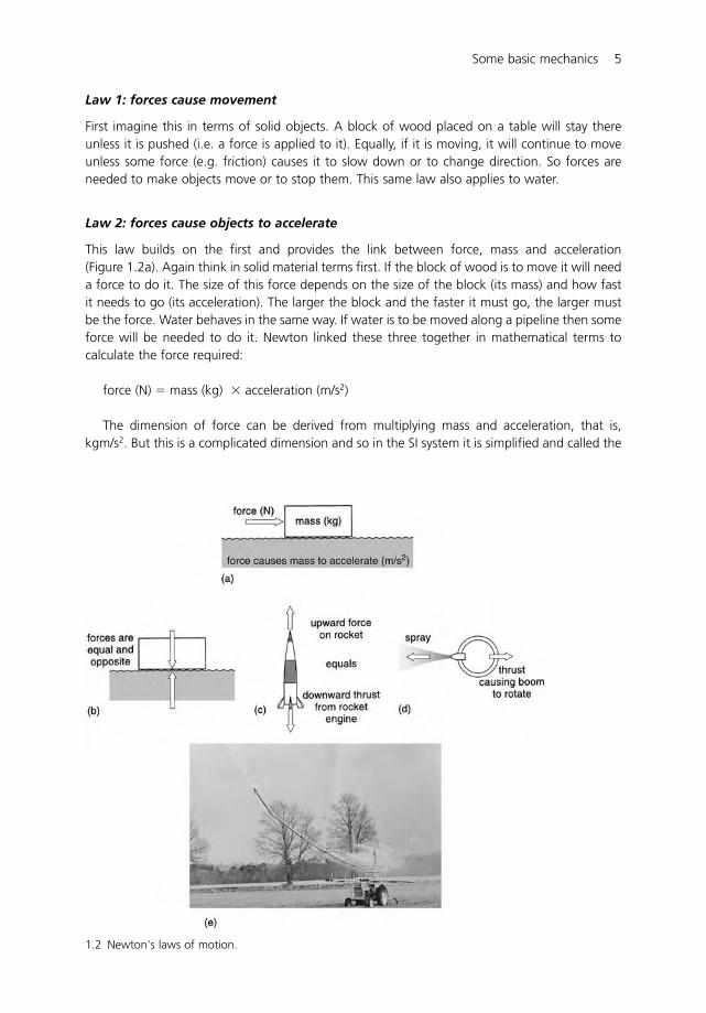
Friction is the name given to the force which resists movement and so causes objects to slowdown (Figure 1.1a). It is an important aspect of all our daily lives. Without friction between ourfeet and the ground surface it would be difficult to walk and we are reminded of this each timewe step onto ice or some smooth oily surface. We would not be able to swim if water wasfrictionless. Our arms would just slide through the water and we would not make any headway –just like children trying to 'swim' in a sea of plastic balls in the playground (Figure 1.1b).
Friction is an essential part of our existence but sometimes it can be a nuisance. In carengines, for example, friction between the moving parts would cause them to quickly heat upand the engine would seize up. But oil lubricates the surfaces and reduces the friction.
Friction also occurs in pipes and channels between flowing water and the internal surface ofa pipe or the bed and sides of a channel. Indeed, much of pipe and channel hydraulics isconcerned with predicting this friction force so that the right size of pipe or channel can bechosen to carry a given flow (see Chapter 4 Pipes and Chapter 5 Channels).

Friction is not only confined to boundaries, there is also friction inside fluids (internal friction)which makes some fluids flow more easily than others. The term viscosity is used to describe thisinternal friction (see Section 1.13.3).
1.6 Newton's laws of motion
Sir Isaac Newton (1642–1728) was one of the first to begin the study of forces and how they causemovement. His work is now enshrined in three basic rules known as Newton's laws of motion.They are very simple laws and at first sight they appear so obvious, they seem hardly worth writ-ing down. But they form the basis of all our understanding of hydraulics (and movement of solidobjects as well) and it took the genius of Newton to recognise their importance.
4 Some basic mechanics
1.1 (a) Friction resists movement and (b) Trying to 'swim in a frictionless fluid'.
Law 1: forces cause movement
First imagine this in terms of solid objects. A block of wood placed on a table will stay thereunless it is pushed (i.e. a force is applied to it). Equally, if it is moving, it will continue to moveunless some force (e.g. friction) causes it to slow down or to change direction. So forces areneeded to make objects move or to stop them. This same law also applies to water.
Law 2: forces cause objects to accelerate
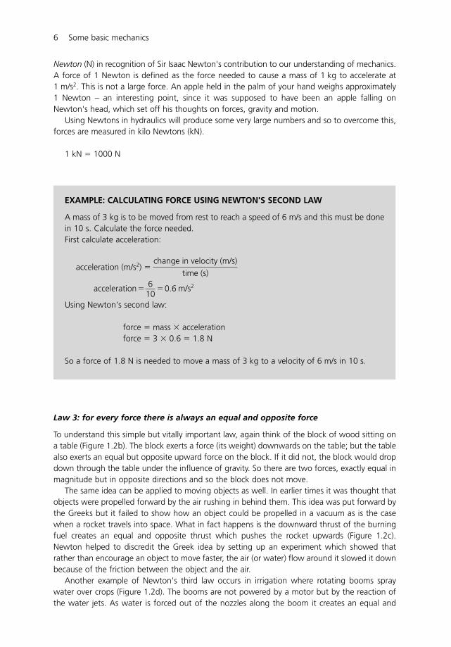
This law builds on the first and provides the link between force, mass and acceleration(Figure 1.2a). Again think in solid material terms first. If the block of wood is to move it will needa force to do it. The size of this force depends on the size of the block (its mass) and how fastit needs to go (its acceleration). The larger the block and the faster it must go, the larger mustbe the force. Water behaves in the same way. If water is to be moved along a pipeline then someforce will be needed to do it. Newton linked these three together in mathematical terms tocalculate the force required:
force (N) � mass (kg) � acceleration (m/s2)
The dimension of force can be derived from multiplying mass and acceleration, that is,kgm/s2. But this is a complicated dimension and so in the SI system it is simplified and called the
Some basic mechanics 5
1.2 Newton's laws of motion.
Newton (N) in recognition of Sir Isaac Newton's contribution to our understanding of mechanics.A force of 1 Newton is defined as the force needed to cause a mass of 1 kg to accelerate at1 m/s2. This is not a large force. An apple held in the palm of your hand weighs approximately1 Newton – an interesting point, since it was supposed to have been an apple falling onNewton's head, which set off his thoughts on forces, gravity and motion.
Using Newtons in hydraulics will produce some very large numbers and so to overcome this,forces are measured in kilo Newtons (kN).
1 kN � 1000 N
6 Some basic mechanics
EXAMPLE: CALCULATING FORCE USING NEWTON'S SECOND LAW
A mass of 3 kg is to be moved from rest to reach a speed of 6 m/s and this must be donein 10 s. Calculate the force needed.First calculate acceleration:
Using Newton's second law:
force � mass � accelerationforce � 3 � 0.6 � 1.8 N
So a force of 1.8 N is needed to move a mass of 3 kg to a velocity of 6 m/s in 10 s.
acceleration � 610
� 0.6 m/s2
acceleration (m/s2) � change in velocity (m/s)
time (s)
Law 3: for every force there is always an equal and opposite force
To understand this simple but vitally important law, again think of the block of wood sitting ona table (Figure 1.2b). The block exerts a force (its weight) downwards on the table; but the tablealso exerts an equal but opposite upward force on the block. If it did not, the block would dropdown through the table under the influence of gravity. So there are two forces, exactly equal inmagnitude but in opposite directions and so the block does not move.
The same idea can be applied to moving objects as well. In earlier times it was thought thatobjects were propelled forward by the air rushing in behind them. This idea was put forward bythe Greeks but it failed to show how an object could be propelled in a vacuum as is the casewhen a rocket travels into space. What in fact happens is the downward thrust of the burningfuel creates an equal and opposite thrust which pushes the rocket upwards (Figure 1.2c).Newton helped to discredit the Greek idea by setting up an experiment which showed thatrather than encourage an object to move faster, the air (or water) flow around it slowed it downbecause of the friction between the object and the air.
Another example of Newton's third law occurs in irrigation where rotating booms spraywater over crops (Figure 1.2d). The booms are not powered by a motor but by the reaction ofthe water jets. As water is forced out of the nozzles along the boom it creates an equal and
opposite force on the boom itself which causes it to rotate. The same principle is used to drivethe water distrubutors on the circular water-cleaning filters at the sewage works.
1.7 Mass and weight
There is often confusion between mass and weight and this has not been helped by the systemof units used in the past. It is also not helped by our common use of the terms in everydaylanguage. Mass and weight have very specific scientific meanings and for any study of water itis essential to have a clear understanding of the difference between them.
Mass refers to an amount of matter or material. It is a constant value and is measured inkilograms (kg). A specific quantity of matter is often referred to as an object. Hence the use ofthis term in the earlier description of Newton's laws.
Weight is a force. Weight is a measure of the force of gravity on an object and this will bedifferent from place to place depending on the gravity. On the earth there are only slightvariations in gravity, but the gravity on the moon is much less than it is on the earth. So the massof an object on the moon would be the same as it is on the earth but its weight would be muchless. As weight is a force, it is measured in Newtons. This clearly distinguishes it from mass whichis measured in kilograms.
Newton's second law also links mass and weight and in this case the acceleration term is theacceleration resulting from gravity. This is the acceleration that any object experiences whendropped and allowed to fall to the earth's surface. Objects dropped in the atmosphere do, infact, experience different rates of acceleration because of the resistance of the air – hence thereason why a feather falls more slowly than a coin. But if both were dropped at the same timein a vacuum they would fall (accelerate) at the same rate. There are also minor variations overthe earth's surface and this is the reason why athletes can sometimes run faster or throw thejavelin further in some parts of the world. However, for engineering purposes, acceleration dueto gravity is assumed to have a constant value of 9.81 m/s2 – usually called the gravity constantand denoted by the letter g. The following equation based on Newton's second law providesthe link between weight and mass:
weight (N) � mass (kg) � gravity constant (m/s2)
Some basic mechanics 7
EXAMPLE: CALCULATING THE WEIGHT OF AN OBJECT
Calculate the weight of an object when its mass is 5 kg.Using Newton's second law:
weight � mass � gravity constantweight � 5 � 9.81 � 49.05 N
Sometimes engineers assume that the gravity constant is 10 m/s2 because it is easier tomultiply by 10 and the error involved in this is not significant in engineering terms.In this case:
weight � 5 � 10 � 50 N
Confusion between mass and weight occurs in our everyday lives. When visiting a shop andasking for 5 kg of potatoes these are duly weighed out on a weigh balance. To be strictly correctwe should ask for 50 N of potatoes, as the balance is measuring the weight of the potatoes (i.e.the force of gravity) and not their mass. But because gravity acceleration is constant all over theworld (or nearly so for most engineering purposes) the conversion factor between mass andweight is a constant value. So the shopkeeper's balance will most likely show kilograms and notNewtons. If shopkeepers were to change their balances to read in Newtons to resolve a scientificconfusion, engineers and scientists might be happy but no doubt a lot of shoppers would notbe so happy!
1.8 Scalar and vector quantities
Measurements in hydraulics are either called scalar or vector quantities. Scalar measurementsonly indicate magnitude. Examples of this are mass, volume, area and length. So if there are120 boxes in a room and they each have a volume of 2 m3 both the number of boxes and thevolume of each are scalar quantities.
Vectors have direction as well as magnitude. Examples of vectors include force and velocity.It is just as important to know which direction forces are pushing and water is moving as wellas their magnitude.
1.9 Dealing with vectors
Scalar quantities can be added together by following the rules of arithmetic. Thus, 5 boxes and4 boxes can be added to make 9 boxes and 3 m and 7 m can be added to make 10 m.
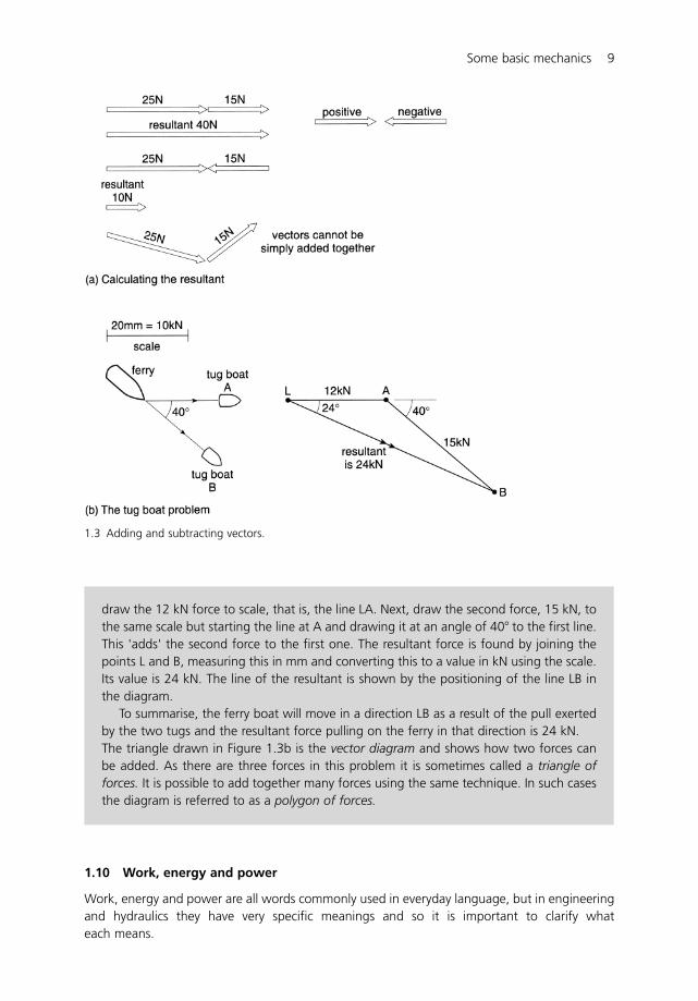
Vectors can also be added together provided their direction is taken into account. Theaddition (or subtraction) of two or more vectors results in another single vector called theresultant and the vectors that make up the resultant are called the components. If two forces,25 N and 15 N, are pushing in the same direction then their resultant is found simply by addingthe two together, that is, 40 N (Figure 1.3a). If they are pushing in opposite directions then theirresultant is found by subtracting them, that is, 10 N. So one direction is considered positive andthe opposite direction negative for the purposes of combining vectors.
But forces can also be at an angle to each other and in such cases a different way of addingor subtracting them is needed – a vector diagram is used for this purpose. This is a diagramdrawn to a chosen scale to show both the magnitude and the direction of the vectors and hencethe magnitude of the resultant vector. An example of how this is done is shown in the box.
Vectors can also be added and subtracted mathematically but a knowledge of trigonometryis needed. For those interested in this approach, it is described in most basic books on mathsand mechanics.
8 Some basic mechanics
EXAMPLE: CALCULATING THE RESULTANT FORCE USING A VECTOR DIAGRAM
Two tug boats A and B are pulling a large ferry boat into a harbour. Tug A is pulling witha force of 12 kN, tug B with a force of 15 kN and the angle between the two tow ropesis 40� (Figure 1.3b). Calculate the resultant force and show the direction in which the ferryboat will move.
First draw a diagram of the ferry and the two tugs. Then, assuming a scale of 40 mmequals 10 kN (this is chosen so that the diagram fits conveniently onto a sheet of paper)
1.10 Work, energy and power
Work, energy and power are all words commonly used in everyday language, but in engineeringand hydraulics they have very specific meanings and so it is important to clarify whateach means.
Some basic mechanics 9
1.3 Adding and subtracting vectors.
draw the 12 kN force to scale, that is, the line LA. Next, draw the second force, 15 kN, tothe same scale but starting the line at A and drawing it at an angle of 40� to the first line.This 'adds' the second force to the first one. The resultant force is found by joining thepoints L and B, measuring this in mm and converting this to a value in kN using the scale.Its value is 24 kN. The line of the resultant is shown by the positioning of the line LB inthe diagram.
To summarise, the ferry boat will move in a direction LB as a result of the pull exertedby the two tugs and the resultant force pulling on the ferry in that direction is 24 kN.The triangle drawn in Figure 1.3b is the vector diagram and shows how two forces canbe added. As there are three forces in this problem it is sometimes called a triangle offorces. It is possible to add together many forces using the same technique. In such casesthe diagram is referred to as a polygon of forces.
1.10.1 Work
Work refers to almost any kind of physical activity but in engineering it has a very specific meaning.Work is done when a force produces movement. A crane does work when it lifts a load againstthe force of gravity and a train does work when it pulls trucks. But if you hold a large weight fora long period of time you will undoubtedly get very tired and feel that you have done a lot of workbut you will not have done any work at all in an engineering sense because nothing moved.
Work done on an object can be calculated as follows:
work done (Nm) � force (N) � distance moved by the object (m)
Work done is the product of force (N) and distance (m) so it is measured in Newton-metres(Nm).
1.10.2 Energy
Energy enables useful work to be done. People and animals require energy to do work. They getthis by eating food and converting it into useful energy for work through the muscles of thebody. Energy is also needed to make water flow and this is why reservoirs are built inmountainous areas so that the natural energy of water can be used to make it flow downhill toa town or to a hydro-electric power station. In many cases energy must be added to water tolift it from a well or a river. This can be supplied by a pumping device driven by a motor usingenergy from fossil fuels such as diesel or petrol. Solar and wind energy are alternatives and sois energy provided by human hands or animals.
The amount of energy needed to do a job is determined by the amount of work to be done.So that:
energy required � work doneso
energy required (Nm) � force (N) � distance (m)
Energy, like work, is measured in Newton-metres (Nm) but the more conventionalmeasurement of energy is watt-seconds (Ws) where:
1 Ws � 1 Nm
But this is a very small quantity for engineers to use and so rather than calculate energy inlarge numbers of Newton-metres or watt-seconds they prefer to use watt-hours (Wh) or kilowatt-hours (kWh). So multiply both sides of this equation by 3600 to change seconds to hours:
1 Wh � 3600 Nm
Now multiply both sides by 1000 to change watts-hours to kilowatt-hours (Wh to kWh):
1 kWh � 3 600 000 Nm� 3600 kNm
Just to add to the confusion some scientists measure energy in joules (J). This is in recognitionof the contribution made by the English physicist, James Joule (1818–1889) to our understandingof energy, in particular, the conversion of mechanical energy to heat energy (see next section).
10 Some basic mechanics
So for the record:
1 joule � 1 Nm
To avoid confusion the term joule is not used in this text. Some everyday examples of energy useinclude:
� A farmer working in the field uses 0.2–0.3 kWh every day.� An electric desk fan uses 0.3 kWh every hour.� An air-conditioner uses 1 kWh every hour.
Notice how it is important to specify the time period (e.g. every hour, every day) overwhich the energy is used. Energy used for pumping water is discussed more fully inChapter 8.
1.10.2.1 Changing energy
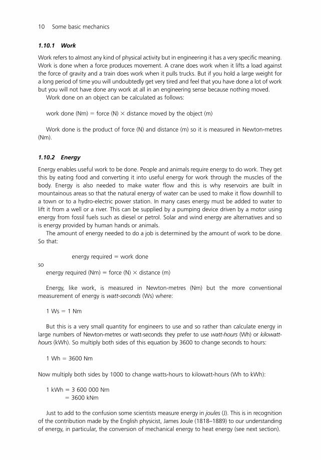
An important aspect of energy is that it can be changed from one form to another. Peopleand animals are able to convert food into useful energy to drive their muscles. The farmer using0.2 kWh every day, for example, must eat enough food each day to supply this energy needotherwise the farmer would not be able to work properly. In a typical diesel engine pumpingsystem, the energy is changed several times before it gets to the water. Chemical energycontained within the fuel (e.g. diesel oil) is burnt in a diesel engine to produce mechanicalenergy. This is converted to useful water energy via the drive shaft and pump (Figure 1.4). Soa pumping unit is both an energy converter as well as a device for adding energy into a watersystem.
The system of energy transfer is not perfect and energy losses occur through friction betweenthe moving parts and is usually lost as heat energy. These losses can be significant and costly interms of fuel use. For this reason it is important to match a pump and its power unit with thejob to be done to maximise the efficiency of energy use (see Chapter 8).
Some basic mechanics 11
1.4 Changing energy from one form to another.
1.10.3 Power
Power is often confused with the term energy. They are related but they have differentmeanings. Whilst energy is the capacity to do useful work, power is the rate at which the energyis used (Figure 1.5).And so:
Examples of power requirements, a typical room air-conditioner has a power rating of 3 kW.This means that it consumes 3 kWh of energy every hour it is working. A small electric radiatorhas a rating of 1–2 kW and the average person walking up and down stairs has a powerrequirement of about 70 W.
Energy requirements are sometimes calculated from knowing the equipment power rating and the time over which it is used rather than trying to calculate it from the work done.In this case:
energy (kWh) � power (kW) � time (h)
Horse Power (HP) is still a very commonly used measure of power but it is not used in thisbook, as it is not an SI unit. However, for the record:
1 kW � 1.36 HP
Power used for pumping water is discussed more fully in Chapter 8.
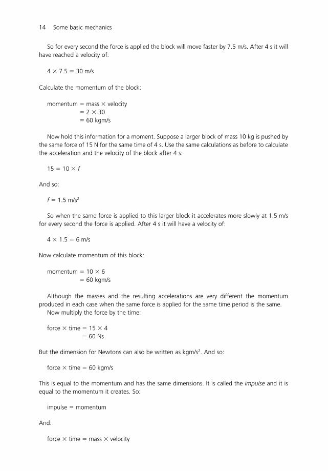
1.11 Momentum
Applying a force to a mass causes it to accelerate (Newton's second law) and the effect of thisis to cause a change in velocity. This means there is a link between mass and velocity and this iscalled momentum. Momentum is another scientific term that is used in everyday language todescribe something that is moving – we say that some object or a football game has momentumif it is moving along and making good progress. In engineering terms it has a specific meaningand it can be calculated by multiplying the mass and the velocity together:
momentum (kgm/s) � mass (kg) � velocity (m/s)
Note the dimensions of momentum are a combination of those of velocity and mass.The following example demonstrates the links between force, mass and velocity. Figure 1.6
shows two blocks that are to be pushed along by applying a force to them. Imagine that thesliding surface is very smooth and so there is no friction.
power (kW) � energy (kWh)
time (h)
12 Some basic mechanics
1.5 Power is the rate of energy use.
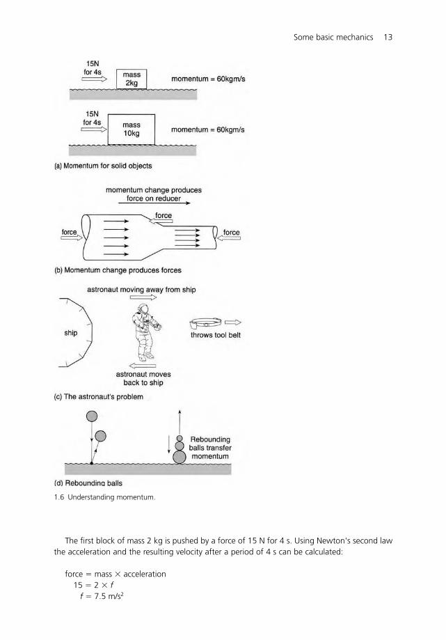
The first block of mass 2 kg is pushed by a force of 15 N for 4 s. Using Newton's second lawthe acceleration and the resulting velocity after a period of 4 s can be calculated:
force � mass � acceleration15 � 2 � f
f � 7.5 m/s2
Some basic mechanics 13
1.6 Understanding momentum.
So for every second the force is applied the block will move faster by 7.5 m/s. After 4 s it willhave reached a velocity of:
4 � 7.5 � 30 m/s
Calculate the momentum of the block:
momentum � mass � velocity� 2 � 30� 60 kgm/s
Now hold this information for a moment. Suppose a larger block of mass 10 kg is pushed bythe same force of 15 N for the same time of 4 s. Use the same calculations as before to calculatethe acceleration and the velocity of the block after 4 s:
15 � 10 � f
And so:
f � 1.5 m/s2
So when the same force is applied to this larger block it accelerates more slowly at 1.5 m/sfor every second the force is applied. After 4 s it will have a velocity of:
4 � 1.5 � 6 m/s
Now calculate momentum of this block:
momentum � 10 � 6� 60 kgm/s
Although the masses and the resulting accelerations are very different the momentumproduced in each case when the same force is applied for the same time period is the same.
Now multiply the force by the time:
force � time � 15 � 4� 60 Ns
But the dimension for Newtons can also be written as kgm/s2. And so:
force � time � 60 kgm/s
This is equal to the momentum and has the same dimensions. It is called the impulse and it isequal to the momentum it creates. So:
impulse � momentum
And:
force � time � mass � velocity
14 Some basic mechanics
This is more commonly written as:
impulse � change of momentum
Writing 'change in momentum' is more appropriate because an object need not be startingfrom rest – it may already be moving. In such cases the object will have some momentum andan impulse would be increasing (changing) it. A momentum change need not be just a changein velocity but also a change in mass. If a lorry loses some of its load when travelling at speedits mass will change. In this case the lorry would gain speed as a result of being smaller in mass,the momentum before being equal to the momentum after the loss of load.
The equation for momentum change becomes:
force � time � mass � change in velocity
This equation works well for solid blocks which are forced to move but it is not easily appliedto flowing water in its present form. For water it is better to look at the rate at which the watermass is flowing rather than thinking of the flow as a series of discrete solid blocks of water. Thisis done by dividing both sides of the equation by time:
Mass divided by time is the mass flow in kg/s and so the equation becomes:
force (N) � mass flow (kg/s) � change in velocity (m/s)
So when flowing water undergoes a change of momentum either by a change in velocity ora change in mass flow (e.g. water flowing around a pipe bend or through a reducer) then a forceis produced by that change (Figure 1.6b). Equally if a force is applied to water (e.g. in a pumpor turbine) then the water will experience a change in momentum.
As momentum is about forces and velocities the direction in which momentum changes is alsoimportant. In the simple force example, the forces are pushing from left to right and so the move-ment is from left to right. This is assumed to be the positive direction. Any force or movement fromright to left would be considered negative. So if several forces are involved they can be added orsubtracted to find a single resultant force. Another important point to note is that Newton's thirdlaw also applies to momentum. The force on the reducer (Figure 1.6b) could be drawn in eitherdirection. In the diagram the force is shown in the negative direction (right to left) and this is theforce that the reducer exerts on the water. Equally it could be drawn in the opposite direction, thatis, the positive direction (left to right) when it would be the force of the water on the reducer.Either way the two forces are equal and opposite as Newton’s third law states.
The application of this idea to water flow is developed further in Section 4.1.3.Those not so familiar with Newton's laws might find momentum more difficult to deal with
than other aspects of hydraulics. To help understand the concept here are two interestingexamples of momentum change which may help.
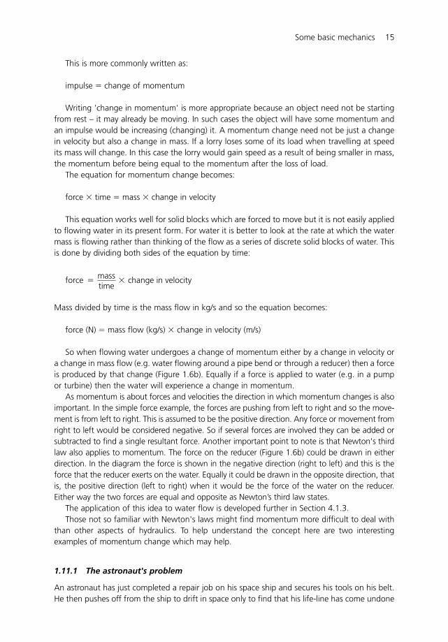
1.11.1 The astronaut's problem
An astronaut has just completed a repair job on his space ship and secures his tools on his belt.He then pushes off from the ship to drift in space only to find that his life-line has come undone
force � masstime
� change in velocity
Some basic mechanics 15
and he is drifting further and further away from his ship (Figure 1.6c). How can he get back? Hecould radio for help, but another solution would be to take off his tool belt and throw it as hardas he can in the direction he is travelling. The reaction from this will be to propel him in theopposite direction and back to his space ship. The momentum created by throwing the tool beltin one direction (i.e. mass of tool belt multiplied by velocity of tool belt) will be matched bymomentum in the opposite direction (i.e. mass of spaceman multiplied by velocity of spaceman).His mass will be much larger than the tool belt and so his velocity will be smaller but at least itwill be in the right direction!
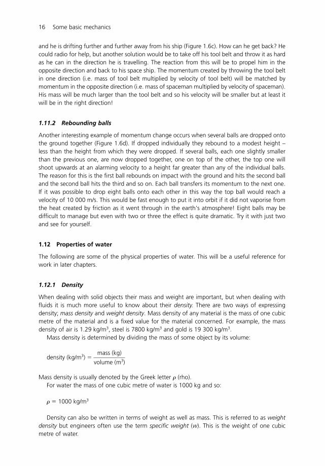
1.11.2 Rebounding balls
Another interesting example of momentum change occurs when several balls are dropped ontothe ground together (Figure 1.6d). If dropped individually they rebound to a modest height –less than the height from which they were dropped. If several balls, each one slightly smallerthan the previous one, are now dropped together, one on top of the other, the top one willshoot upwards at an alarming velocity to a height far greater than any of the individual balls.The reason for this is the first ball rebounds on impact with the ground and hits the second balland the second ball hits the third and so on. Each ball transfers its momentum to the next one.If it was possible to drop eight balls onto each other in this way the top ball would reach avelocity of 10 000 m/s. This would be fast enough to put it into orbit if it did not vaporise fromthe heat created by friction as it went through in the earth's atmosphere! Eight balls may bedifficult to manage but even with two or three the effect is quite dramatic. Try it with just twoand see for yourself.
1.12 Properties of water
The following are some of the physical properties of water. This will be a useful reference forwork in later chapters.
1.12.1 Density
When dealing with solid objects their mass and weight are important, but when dealing withfluids it is much more useful to know about their density. There are two ways of expressingdensity; mass density and weight density. Mass density of any material is the mass of one cubicmetre of the material and is a fixed value for the material concerned. For example, the massdensity of air is 1.29 kg/m3, steel is 7800 kg/m3 and gold is 19 300 kg/m3.
Mass density is determined by dividing the mass of some object by its volume:
Mass density is usually denoted by the Greek letter � (rho).For water the mass of one cubic metre of water is 1000 kg and so:
� � 1000 kg/m3
Density can also be written in terms of weight as well as mass. This is referred to as weightdensity but engineers often use the term specific weight (w). This is the weight of one cubicmetre of water.
density (kg/m3) � mass (kg)
volume (m3)
16 Some basic mechanics
Newton's second law is used to link mass and weight:
weight density (kN/m3) � mass density (kg/m3) � gravity constant (m/s2)
For water:
weight density � 1000 � 9.81� 9810 N/m3 (or 9.81 kN/m3)� 10 kN/m3 (approximately)
Sometimes weight density for water is rounded off by engineers to 10 kN/m3. Usually thismakes very little difference to the design of most hydraulic works. Note the equation for weightdensity is applicable to all fluids and not just water. It can be used to find the weight density ofany fluid provided the mass density is known.
Engineers generally use the term specific weight in their calculations whereas scientists tendto use the term �g to describe the weight density. They are in effect the same but for clarity,�g is used throughout this book.
1.12.2 Relative density or specific gravity
Sometimes it is more convenient to use relative density rather than just density. It is morecommonly referred to as specific gravity and is the ratio of the density of a material or fluid tothat of some standard density – usually water. It can be written both in terms of the mass densityand the weight density.
Note that specific gravity has no dimensions. As the volume is the same for both the objectand the water, another way of writing this formula is in terms of weight:
Some useful specific gravity values are included in Table 1.3.The density of any other fluid (or any solid object) can be calculated by knowing the specific
gravity. The mass density of mercury, for example, can be calculated from its specific gravity:
specific gravity of mercury (SG) � mass density of mercury (kg/m3)
mass density of water (kg/m3)
specific gravity � weight of an object
weight of an equal volume of water
specific gravity (SG) � density of an object (kg/m3)
density of water (kg/m3)
Some basic mechanics 17
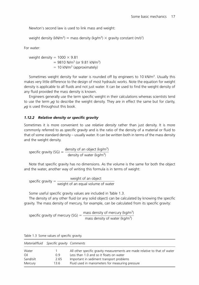
Table 1.3 Some values of specific gravity.
Material/fluid Specific gravity Comments
Water 1 All other specific gravity measurements are made relative to that of waterOil 0.9 Less than 1.0 and so it floats on waterSand/silt 2.65 Important in sediment transport problemsMercury 13.6 Fluid used in manometers for measuring pressure
So:
mass density of mercury � SG of mercury � mass density of water� 13.6 � 1000� 13 600 kg/m3
The mass density of mercury is 13.6 times greater than that of water.Archimedes used this concept of specific gravity in his famous principle (Table 1.3), which is
discussed in Section 2.12.
1.12.3 Viscosity
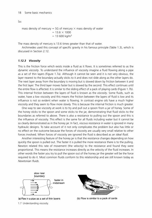
This is the friction force which exists inside a fluid as it flows. It is sometimes referred to as thedynamic viscosity. To understand the influence of viscosity imagine a fluid flowing along a pipeas a set of thin layers (Figure 1.7a). Although it cannot be seen and it is not very obvious, thelayer nearest to the boundary actually sticks to it and does not slide along as the other layers do.The next layer away from the boundary is moving but is slowed down by friction between it andthe first layer. The third layer moves faster but is slowed by the second. This effect continues untilthe entire flow is affected. It is similar to the sliding effect of a pack of playing cards (Figure 1.7b).This internal friction between the layers of fluid is known as the viscosity. Some fluids, such aswater, have a low viscosity and this means the friction between the layers of fluid is low and itsinfluence is not so evident when water is flowing. In contrast engine oils have a much higherviscosity and they seem to flow more slowly. This is because the internal friction is much greater.
One way to see viscosity at work is to try and pull out a spoon from a jar of honey. Some ofthe honey sticks to the spoon and some sticks to the jar, demonstrating that fluid sticks to theboundaries as referred to above. There is also a resistance to pulling out the spoon and this isthe influence of viscosity. This effect is the same for all fluids including water but it cannot beso clearly demonstrated as in the honey jar. In fact, viscous resistance in water is ignored in manyhydraulic designs. To take account of it not only complicates the problem but also has little orno effect on the outcome because the forces of viscosity are usually very small relative to otherforces involved. When forces of viscosity are ignored the fluid is described as an ideal fluid.
Another interesting feature of the honey jar is that the resistance changes depending on howquickly the spoon is pulled out. The faster it is pulled the more resistance there is to the pulling.Newton related this rate of movement (the velocity) to the resistance and found they wereproportional. This means the resistance increases directly as the velocity of the fluid increases. Inother words the faster you try to pull the spoon out of the honey jar the greater will be the forcerequired to do it. Most common fluids conform to this relationship and are still known today asNewtonian fluids.
18 Some basic mechanics
1.7 Understanding viscosity.
Some modern fluids however, have different viscous properties and are called non-Newtonianfluids. One good example is tomato ketchup. When left on the shelf it is a highly viscous fluidwhich does not flow easily from the bottle. Sometimes you can turn a full bottle upside downand nothing comes out. But shake it vigorously (in scientific terms this means applying a shearforce) its viscosity suddenly changes and the ketchup flows easily from the bottle. In other words,applying a force to a fluid can change its viscous properties often to our advantage.
Although viscosity is often ignored in hydraulics, life would be difficult without it. The spoonin the honey jar would come out clean and it would be difficult to get the honey out of the jar.Rivers rely on viscosity to slow down flows otherwise they would continue to accelerate to veryhigh speeds. The Mississippi river would reach a speed of over 300 km/h as its flow graduallydescends 450 m towards the sea if water had no viscosity. Pumps would not work becauseimpellers would not be able to grip the water and swimmers would not be able to propelthemselves through the water for the same reason.
Viscosity is usually denoted by the Greek letter (mu).For water:
� � 0.00114 kg/ms at a temperature of 15�C� 1.14 � 103 kg/ms
The viscosity of all fluids is influenced by temperature. Viscosity decreases with increasingtemperature.
1.12.4 Kinematic viscosity
In many hydraulic calculations viscosity and mass density go together and so they are oftencombined into a term known as the kinematic viscosity. It is denoted by the Greek letter (nu)and is calculated as follows:
For water:
� � 1.14 � 10�2 m2/s at a temperature of 15�C
Sometimes kinematic viscosity is measured in Stokes in recognition of the work of Sir GeorgeStokes who helped to develop a fuller understanding of the role of viscosity in fluids.
104 Stokes � 1 m2/s
For water:
� � 1.14 � 10�2 Stokes
1.12.5 Surface tension
An ordinary steel sewing needle can be made to float on water if it is placed there very carefully.A close examination of the water surface around the needle shows that it appears to be sittingin a slight depression and the water behaves as if it is covered with an elastic skin. This property
kinematic viscosity (�) � viscosity (�)
density (�)
Some basic mechanics 19
is known as surface tension. The force of surface tension is very small and is normally expressedin terms of force per unit length.
For water:
surface tension � 0.51 N/m at a temperature of 20�C
This force is ignored in most hydraulic calculations but in hydraulic modelling, where small-scalemodels are constructed in a laboratory to try and work out forces and flows in large, complexproblems, surface tension may influence the outcome because of the small water depths andflows involved.
1.12.6 Compressibility
It is easy to imagine a gas being compressible and to some extent some solid materials such asrubber. In fact all materials are compressible to some degree including water which is 100 timesmore compressible than steel! The compressibility of water is important in many aspects ofhydraulics. Take for example the task of closing a sluice valve to stop water flowing along apipeline. If the water was incompressible it would be like trying to stop a solid 40 ton truck. Thewater column would be a solid mass running into the valve and the force of impact could besignificant. Fortunately water is compressible and as it impacts on the valve it compresses like aspring and this absorbs the energy of the impact. Returning to the road analogy, it is similar towhat happens when cars crash on the road because of some sudden stoppage. Each carcollapses on impact and this absorbs much of the energy of the collision. However, this is notthe end of the story. As the water compresses the energy that is absorbed causes the waterpressure to suddenly rise and this leads to another problem known as water hammer. This isdiscussed more fully in Section 4.16.
20 Some basic mechanics

2 Hydrostatics: water at rest
2.1 Introduction
Hydrostatics is the study of water which is not moving, that is, it is at rest. It is important to civilengineers for the design of water storage tanks and dams. What are the forces created by waterand how strong must a tank or a dam be to resist them? It is also important to naval architectswho design ships and submarines. How deep can a submarine go before the pressures becometoo great and damage it? The answers to these questions can be found from studyinghydrostatics. The theory is quite simple both in concept and in use. It is also a well-establishedtheory that was set down by Archimedes (287–212BC) over 2000 years ago and is still used inmuch the same way today.
2.2 Pressure
The term pressure is used to describe the force exerted by water on each square metre of someobject submerged in water, that is, force per unit area. It may be the bottom of a tank, the sideof a dam, a ship or a submerged submarine. It is calculated as follows:
Introducing the units of measurement:
Force is in kilo-Newtons (kN), area is in square metres (m2) and so pressure is measured in kN/m2.Sometimes pressure is measured in Pascals (Pa) in recognition of Blaise Pascal (1620–1662) whoclarified much of modern-day thinking about pressure and barometers for measuringatmospheric pressure.
1 Pa � 1 N/m2
pressure (kN/m2) � force (kN)
area (m2)
pressure � forcearea
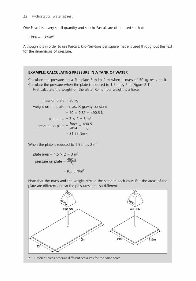
EXAMPLE: CALCULATING PRESSURE IN A TANK OF WATER
Calculate the pressure on a flat plate 3 m by 2 m when a mass of 50 kg rests on it.Calculate the pressure when the plate is reduced to 1.5 m by 2 m (Figure 2.1).
First calculate the weight on the plate. Remember weight is a force.
mass on plate � 50 kg
weight on the plate � mass � gravity constant
� 50 � 9.81 � 490.5 N
plate area � 3 � 2 � 6 m2
pressure on plate � �
� 81.75 N/m2
When the plate is reduced to 1.5 m by 2 m:
plate area � 1.5 � 2 � 3 m2
pressure on plate �
= 163.5 N/m2
Note that the mass and the weight remain the same in each case. But the areas of theplate are different and so the pressures are also different.
490.53
490.56
forcearea
One Pascal is a very small quantity and so kilo-Pascals are often used so that:
1 kPa � 1 kN/m2
Although it is in order to use Pascals, kilo-Newtons per square metre is used throughout this textfor the dimensions of pressure.
22 Hydrostatics: water at rest
2.1 Different areas produce different pressures for the same force.
2.3 Force and pressure are different
Force and pressure are terms that are often confused. The difference between them is bestillustrated by an example. If you had to choose between an elephant standing on your foot ora woman in a high-heel (stiletto) shoe, which would you choose? The sensible answer would bethe elephant, as it is less likely to do damage to your foot than the high-heel shoe. To under-stand this is to appreciate the important difference between force and pressure.
The weight of the elephant is obviously greater than that of the woman but the pressureunder the elephant’s foot is much less than that under the high-heel shoe (see calculations inthe box). The woman’s weight (force) is small in comparison to that of the elephant, but the areaof the shoe heel is very small and so the pressure is extremely high. So the high-heel shoe is likelyto cause you more pain than the elephant. This is why high-heel shoes, particularly those witha very fine heel, are sometimes banned indoors as they can so easily punch holes in flooring andfurniture!
There are many other examples which highlight the difference. Agricultural tractors often usewide (floatation) tyres to spread their load and reduce soil compaction. Military tanks usecaterpillar tracks to spread the load to avoid getting bogged down in muddy conditions. Eskimosuse shoes like tennis rackets to avoid sinking into the soft snow.
Hydrostatics: water at rest 23
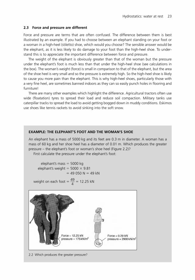
EXAMPLE: THE ELEPHANT’S FOOT AND THE WOMAN’S SHOE
An elephant has a mass of 5000 kg and its feet are 0.3 m in diameter. A woman has amass of 60 kg and her shoe heel has a diameter of 0.01 m. Which produces the greaterpressure – the elephant’s foot or woman’s shoe heel (Figure 2.2)?
First calculate the pressure under the elephant’s foot:
elephant’s mass � 5000 kgelephant’s weight � 5000 � 9.81
� 49 050 N � 49 kN
weight on each foot � � 12.25 kN494
2.2 Which produces the greater pressure?
2.4 Pressure and depth
The pressure on some object under water is determined by the depth of water above it. So thedeeper the object is below the surface, the higher will be the pressure. The pressure can becalculated using the pressure-head equation:
p � �gh
where p is pressure (kN/m2); � is mass density of water (kN/m3); g is gravity constant (m/s2); h isdepth of water (m).
This equation works for all fluids and not just water, provided of course that the correct valueof density is used for the fluid concerned.
To see how the pressure-head equation is derived look in the box below.
24 Hydrostatics: water at rest
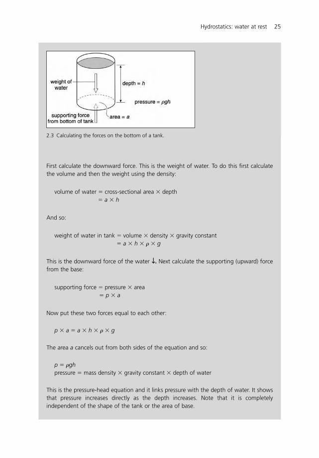
foot area � �
� 0.07 m2
pressure under foot � �
� 175 kN/m2
Now calculate the pressure under the woman’s shoe heel:
woman’s mass � 60 kgwoman’s weight � 589 N � 0.59 kN
weight on each foot � � 0.29 kN
area of shoe heel � �
� 0.0001 m2
pressure under heel � �
� 2900 kN/m2
The pressure under the woman’s heel is 16 times greater than under the elephant’s foot.So which would you rather have standing on your foot?
0.290.0001
forcearea
�0.012
4�d2
4
0.592
12.250.07
forcearea
�0.32
4�d2
4
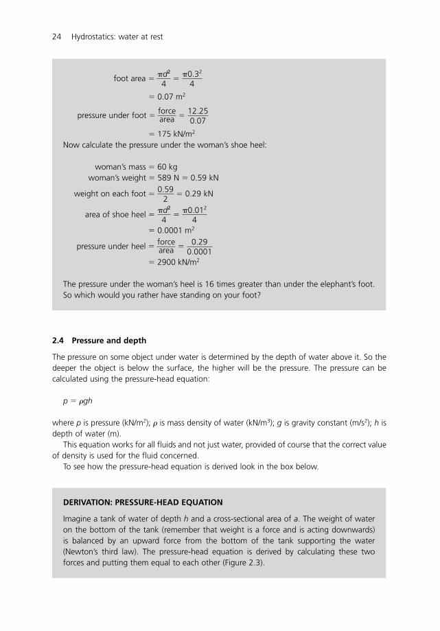
DERIVATION: PRESSURE-HEAD EQUATION
Imagine a tank of water of depth h and a cross-sectional area of a. The weight of wateron the bottom of the tank (remember that weight is a force and is acting downwards)is balanced by an upward force from the bottom of the tank supporting the water(Newton’s third law). The pressure-head equation is derived by calculating these twoforces and putting them equal to each other (Figure 2.3).
Hydrostatics: water at rest 25
First calculate the downward force. This is the weight of water. To do this first calculatethe volume and then the weight using the density:
volume of water � cross-sectional area � depth� a � h
And so:
weight of water in tank � volume � density � gravity constant� a � h � � � g
This is the downward force of the water ↓↓. Next calculate the supporting (upward) forcefrom the base:
supporting force � pressure � area� p � a
Now put these two forces equal to each other:
p � a � a � h � � � g
The area a cancels out from both sides of the equation and so:
p � �ghpressure � mass density � gravity constant � depth of water
This is the pressure-head equation and it links pressure with the depth of water. It showsthat pressure increases directly as the depth increases. Note that it is completelyindependent of the shape of the tank or the area of base.
2.3 Calculating the forces on the bottom of a tank.
2.5 Pressure is same in all directions
Although in the box example the pressure is used to calculate the downward force on the tankbase, pressure does not in fact have a specific direction – it pushes in all directions. Tounderstand this, imagine a cube immersed in water (Figure 2.5). The water pressure pushes onall sides of the cube and not just on the top. If the cube was very small then the pressure on allsix faces would be almost the same. If the cube gets smaller and smaller until it almost disap-pears, it becomes clear that the pressure at any point in the water is the same in all directions.So the pressure pushes in all directions and not just vertically. This idea is important for design-ing dams because it is the horizontal action of pressure which pushes on a dam and which must
26 Hydrostatics: water at rest
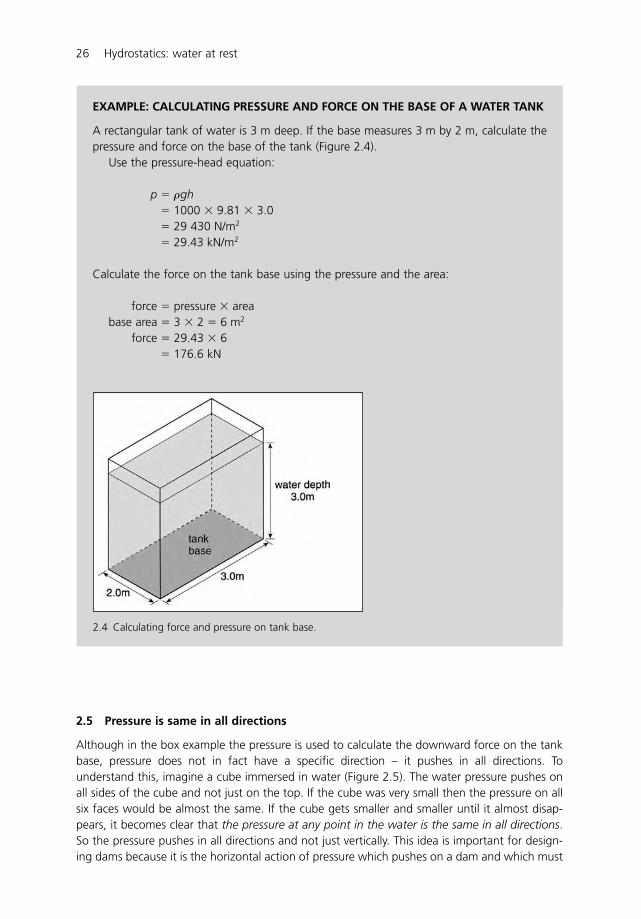
EXAMPLE: CALCULATING PRESSURE AND FORCE ON THE BASE OF A WATER TANK
A rectangular tank of water is 3 m deep. If the base measures 3 m by 2 m, calculate thepressure and force on the base of the tank (Figure 2.4).
Use the pressure-head equation:
p � �gh� 1000 � 9.81 � 3.0� 29 430 N/m2
� 29.43 kN/m2
Calculate the force on the tank base using the pressure and the area:
force � pressure � areabase area � 3 � 2 � 6 m2
force � 29.43 � 6� 176.6 kN
2.4 Calculating force and pressure on tank base.
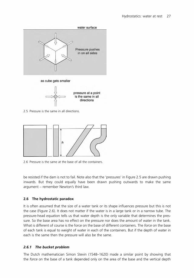
be resisted if the dam is not to fail. Note also that the ‘pressures’ in Figure 2.5 are drawn pushinginwards. But they could equally have been drawn pushing outwards to make the sameargument – remember Newton’s third law.
2.6 The hydrostatic paradox
It is often assumed that the size of a water tank or its shape influences pressure but this is notthe case (Figure 2.6). It does not matter if the water is in a large tank or in a narrow tube. Thepressure-head equation tells us that water depth is the only variable that determines the pres-sure. So the base area has no effect on the pressure nor does the amount of water in the tank.What is different of course is the force on the base of different containers. The force on the baseof each tank is equal to weight of water in each of the containers. But if the depth of water ineach is the same then the pressure will also be the same.
2.6.1 The bucket problem
The Dutch mathematician Simon Stevin (1548–1620) made a similar point by showing thatthe force on the base of a tank depended only on the area of the base and the vertical depth
Hydrostatics: water at rest 27
2.5 Pressure is the same in all directions.
2.6 Pressure is the same at the base of all the containers.
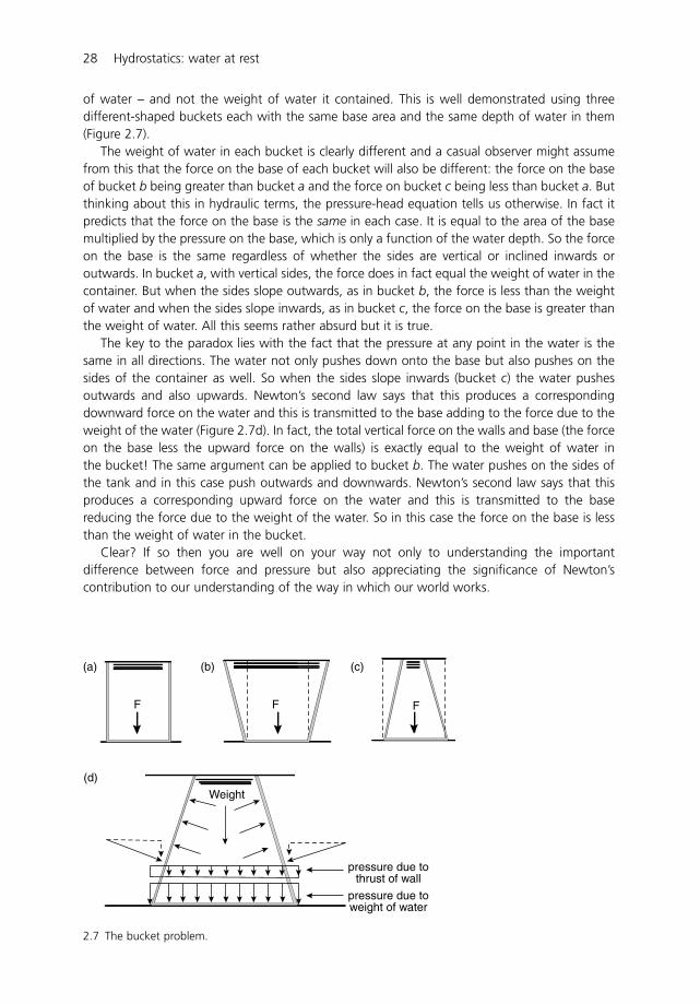
of water – and not the weight of water it contained. This is well demonstrated using threedifferent-shaped buckets each with the same base area and the same depth of water in them(Figure 2.7).
The weight of water in each bucket is clearly different and a casual observer might assumefrom this that the force on the base of each bucket will also be different: the force on the baseof bucket b being greater than bucket a and the force on bucket c being less than bucket a. Butthinking about this in hydraulic terms, the pressure-head equation tells us otherwise. In fact itpredicts that the force on the base is the same in each case. It is equal to the area of the basemultiplied by the pressure on the base, which is only a function of the water depth. So the forceon the base is the same regardless of whether the sides are vertical or inclined inwards oroutwards. In bucket a, with vertical sides, the force does in fact equal the weight of water in thecontainer. But when the sides slope outwards, as in bucket b, the force is less than the weightof water and when the sides slope inwards, as in bucket c, the force on the base is greater thanthe weight of water. All this seems rather absurd but it is true.
The key to the paradox lies with the fact that the pressure at any point in the water is thesame in all directions. The water not only pushes down onto the base but also pushes on thesides of the container as well. So when the sides slope inwards (bucket c) the water pushesoutwards and also upwards. Newton’s second law says that this produces a correspondingdownward force on the water and this is transmitted to the base adding to the force due to theweight of the water (Figure 2.7d). In fact, the total vertical force on the walls and base (the forceon the base less the upward force on the walls) is exactly equal to the weight of water inthe bucket! The same argument can be applied to bucket b. The water pushes on the sides ofthe tank and in this case push outwards and downwards. Newton’s second law says that thisproduces a corresponding upward force on the water and this is transmitted to the basereducing the force due to the weight of the water. So in this case the force on the base is lessthan the weight of water in the bucket.
Clear? If so then you are well on your way not only to understanding the importantdifference between force and pressure but also appreciating the significance of Newton’scontribution to our understanding of the way in which our world works.
28 Hydrostatics: water at rest
(a)
(d)
F F F
Weight
pressure due tothrust of wall
pressure due toweight of water
(b) (c)
2.7 The bucket problem.
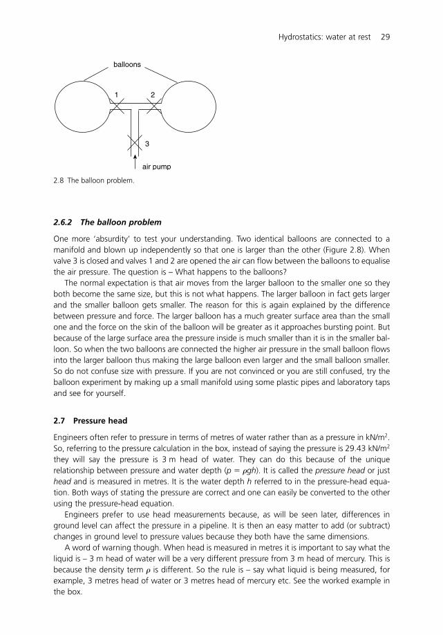
2.6.2 The balloon problem
One more ‘absurdity’ to test your understanding. Two identical balloons are connected to amanifold and blown up independently so that one is larger than the other (Figure 2.8). Whenvalve 3 is closed and valves 1 and 2 are opened the air can flow between the balloons to equalisethe air pressure. The question is – What happens to the balloons?
The normal expectation is that air moves from the larger balloon to the smaller one so theyboth become the same size, but this is not what happens. The larger balloon in fact gets largerand the smaller balloon gets smaller. The reason for this is again explained by the differencebetween pressure and force. The larger balloon has a much greater surface area than the smallone and the force on the skin of the balloon will be greater as it approaches bursting point. Butbecause of the large surface area the pressure inside is much smaller than it is in the smaller bal-loon. So when the two balloons are connected the higher air pressure in the small balloon flowsinto the larger balloon thus making the large balloon even larger and the small balloon smaller.So do not confuse size with pressure. If you are not convinced or you are still confused, try theballoon experiment by making up a small manifold using some plastic pipes and laboratory tapsand see for yourself.
2.7 Pressure head
Engineers often refer to pressure in terms of metres of water rather than as a pressure in kN/m2.So, referring to the pressure calculation in the box, instead of saying the pressure is 29.43 kN/m2
they will say the pressure is 3 m head of water. They can do this because of the uniquerelationship between pressure and water depth (p � �gh). It is called the pressure head or justhead and is measured in metres. It is the water depth h referred to in the pressure-head equa-tion. Both ways of stating the pressure are correct and one can easily be converted to the otherusing the pressure-head equation.
Engineers prefer to use head measurements because, as will be seen later, differences inground level can affect the pressure in a pipeline. It is then an easy matter to add (or subtract)changes in ground level to pressure values because they both have the same dimensions.
A word of warning though. When head is measured in metres it is important to say what theliquid is – 3 m head of water will be a very different pressure from 3 m head of mercury. This isbecause the density term � is different. So the rule is – say what liquid is being measured, forexample, 3 metres head of water or 3 metres head of mercury etc. See the worked example inthe box.
Hydrostatics: water at rest 29
air pump
3
21
balloons
2.8 The balloon problem.
2.8 Atmospheric pressure
The pressure of the atmosphere is all around us pressing on our bodies. Although we often talkabout things being ‘as light as air’ when there is a large depth of air, as on the earth’s surface,it creates a very high pressure of approximately 100 kN/m2. The average person has a skin areaof 2 m2 so the force acting on each of us from the air around us is approximately 200 kN (theequivalent of 200 000 apples or approximately 20 tons). A very large force indeed! Fortunatelythere is an equal and opposite pressure from within our bodies that balances the air pressureand so we feel no effect (Newton’s third law).
At high altitudes where atmospheric pressure is less than at the earth’s surface, some peoplesuffer from nose bleeds due to their blood pressure being much higher than that of thesurrounding atmosphere. We also notice slight, sudden changes in air pressure. For instance,when we fly in an aeroplane, even though the cabin is pressurised, our ears pop as our bodiesadjust to changes in the cabin pressure. But if for some reason the cabin pressure system failedsuddenly removing one side of this pressure balance then the result could be catastrophic. Inertgases such as nitrogen, which are normally dissolved in our body fluids and tissues, wouldrapidly start to form gas bubbles which can result in sensory failure, paralysis and death. Deepsea divers are well aware of this rapid pressure change problem and so make sure that theyreturn to the surface slowly so that their bodies have enough time to adjust to the changingpressure. It is known as ‘the bends’. A good practical demonstration of what happens can beseen when you open a fizzy drink bottle. When the cap is removed from the bottle, gas is heardescaping, and bubbles can be seen forming in the drink. This is carbon dioxide gas coming outof solution as a result of the sudden pressure drop inside the bottle as it equalises with thepressure of the atmosphere.
30 Hydrostatics: water at rest
EXAMPLE: CALCULATING PRESSURE HEAD IN MERCURY
Building on the previous example, calculate the depth of mercury needed in the tank toproduce the same pressure as 3 m depth of water (29.43 kN/m2). Specific gravity (SG) ofmercury is 13.6.
First calculate the density of mercury:
ρ (mercury) � � (water) � SG (mercury)� 1000 � 13.6� 13 600 kg/m3
Use the pressure-head equation to calculate the head of mercury:
p � �gh
Where � is now the density and h is the depth of mercury:
29 430 � 13 600 � 9.81 � hh � 0.22 m of mercury
So the depth of mercury required to create the same pressure as 3 m of water is only0.22 m. This is because mercury is much denser than water.
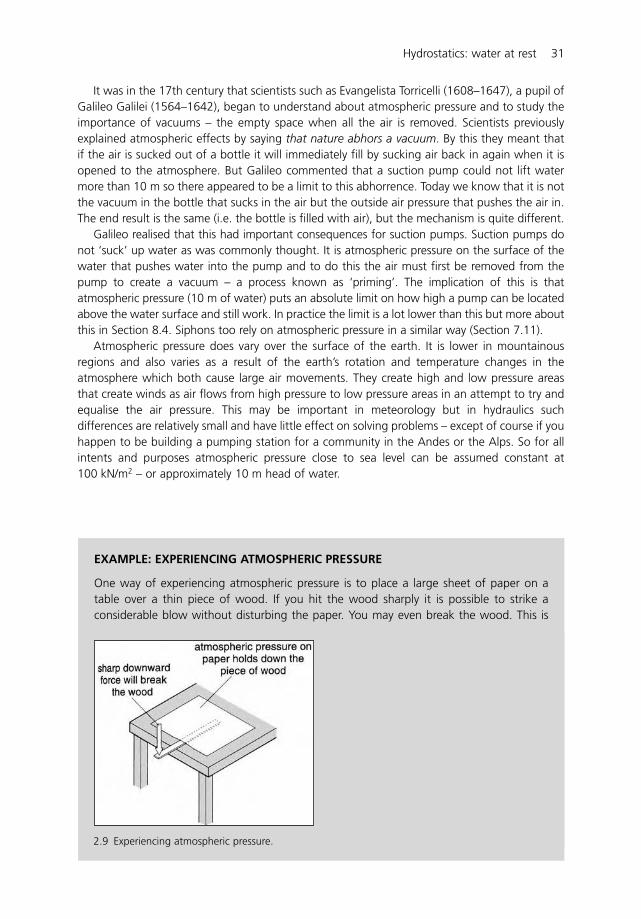
EXAMPLE: EXPERIENCING ATMOSPHERIC PRESSURE
One way of experiencing atmospheric pressure is to place a large sheet of paper on atable over a thin piece of wood. If you hit the wood sharply it is possible to strike aconsiderable blow without disturbing the paper. You may even break the wood. This is
It was in the 17th century that scientists such as Evangelista Torricelli (1608–1647), a pupil ofGalileo Galilei (1564–1642), began to understand about atmospheric pressure and to study theimportance of vacuums – the empty space when all the air is removed. Scientists previouslyexplained atmospheric effects by saying that nature abhors a vacuum. By this they meant thatif the air is sucked out of a bottle it will immediately fill by sucking air back in again when it isopened to the atmosphere. But Galileo commented that a suction pump could not lift watermore than 10 m so there appeared to be a limit to this abhorrence. Today we know that it is notthe vacuum in the bottle that sucks in the air but the outside air pressure that pushes the air in.The end result is the same (i.e. the bottle is filled with air), but the mechanism is quite different.
Galileo realised that this had important consequences for suction pumps. Suction pumps donot ‘suck’ up water as was commonly thought. It is atmospheric pressure on the surface of thewater that pushes water into the pump and to do this the air must first be removed from thepump to create a vacuum – a process known as ‘priming’. The implication of this is thatatmospheric pressure (10 m of water) puts an absolute limit on how high a pump can be locatedabove the water surface and still work. In practice the limit is a lot lower than this but more aboutthis in Section 8.4. Siphons too rely on atmospheric pressure in a similar way (Section 7.11).
Atmospheric pressure does vary over the surface of the earth. It is lower in mountainousregions and also varies as a result of the earth’s rotation and temperature changes in theatmosphere which both cause large air movements. They create high and low pressure areasthat create winds as air flows from high pressure to low pressure areas in an attempt to try andequalise the air pressure. This may be important in meteorology but in hydraulics suchdifferences are relatively small and have little effect on solving problems – except of course if youhappen to be building a pumping station for a community in the Andes or the Alps. So for allintents and purposes atmospheric pressure close to sea level can be assumed constant at100 kN/m2 – or approximately 10 m head of water.
Hydrostatics: water at rest 31
2.9 Experiencing atmospheric pressure.
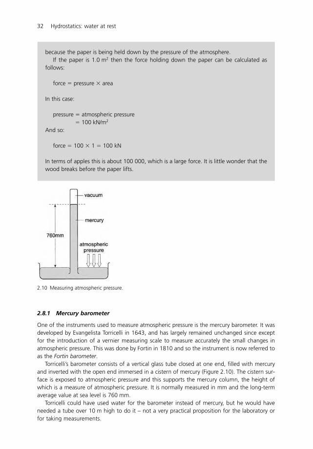
2.8.1 Mercury barometer
One of the instruments used to measure atmospheric pressure is the mercury barometer. It wasdeveloped by Evangelista Torricelli in 1643, and has largely remained unchanged since exceptfor the introduction of a vernier measuring scale to measure accurately the small changes inatmospheric pressure. This was done by Fortin in 1810 and so the instrument is now referred toas the Fortin barometer.
Torricelli’s barometer consists of a vertical glass tube closed at one end, filled with mercuryand inverted with the open end immersed in a cistern of mercury (Figure 2.10). The cistern sur-face is exposed to atmospheric pressure and this supports the mercury column, the height ofwhich is a measure of atmospheric pressure. It is normally measured in mm and the long-termaverage value at sea level is 760 mm.
Torricelli could have used water for the barometer instead of mercury, but he would haveneeded a tube over 10 m high to do it – not a very practical proposition for the laboratory orfor taking measurements.
32 Hydrostatics: water at rest
because the paper is being held down by the pressure of the atmosphere.If the paper is 1.0 m2 then the force holding down the paper can be calculated as
follows:
force � pressure � area
In this case:
pressure � atmospheric pressure� 100 kN/m2
And so:
force � 100 � 1 � 100 kN
In terms of apples this is about 100 000, which is a large force. It is little wonder that thewood breaks before the paper lifts.
2.10 Measuring atmospheric pressure.
Atmospheric pressure is also used as a unit of measurement for pressure both for meteorologicalpurposes and in hydraulics. This unit is known as the bar. For convenience I bar pressure isrounded off to 100 kN/m2.
A more commonly used term in meteorology is the millibar.So:
1 millibar � 0.1 kN/m2 � 100 N/m2
To summarise – there are several ways of expressing atmospheric pressure:
atmospheric pressure � 1 baror � 100 kN/m2
or � 10 m of wateror � 760 mm of mercury
Hydrostatics: water at rest 33
EXAMPLE: MEASURING ATMOSPHERIC PRESSURE USING A MERCURY BAROMETER
Calculate atmospheric pressure when the reading on a mercury barometer is 760 mm ofmercury. What would be the height of the column if the same air pressure was measuredusing water instead of mercury?
The pressure-head equation links together atmospheric pressure and the height of themercury column, but remember the fluid is now mercury and not water:
atmospheric pressure � �gh
h is 760 mm and � for mercury is 13 600 kg/m3 (13.6 times denser than water)
So:
atmospheric pressure � 13 600 � 9.81 � 0.76� 101 400 N/m2 or 101.4 kN/m2
Calculate the height of the water column to measure atmospheric pressure using thepressure-head equation again:
atmospheric pressure � �gh
This time the fluid is water and so:
101 400 � 1000 � 9.81 � hh � 10.32 m
This is a very tall water column and there would be practical difficulties if it was used forroutine measurement of atmospheric pressure. Hence the reason why a very dense liquidlike mercury is used to make measurement more manageable.
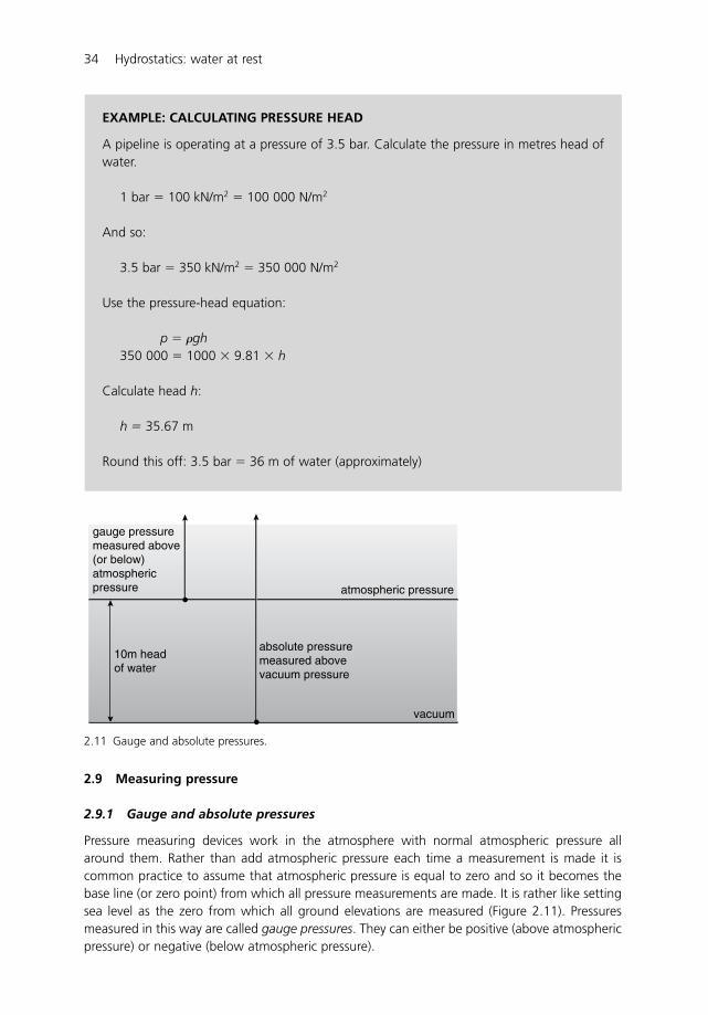
2.9 Measuring pressure
2.9.1 Gauge and absolute pressures
Pressure measuring devices work in the atmosphere with normal atmospheric pressure allaround them. Rather than add atmospheric pressure each time a measurement is made it iscommon practice to assume that atmospheric pressure is equal to zero and so it becomes thebase line (or zero point) from which all pressure measurements are made. It is rather like settingsea level as the zero from which all ground elevations are measured (Figure 2.11). Pressuresmeasured in this way are called gauge pressures. They can either be positive (above atmosphericpressure) or negative (below atmospheric pressure).
34 Hydrostatics: water at rest
EXAMPLE: CALCULATING PRESSURE HEAD
A pipeline is operating at a pressure of 3.5 bar. Calculate the pressure in metres head ofwater.
1 bar � 100 kN/m2 � 100 000 N/m2
And so:
3.5 bar � 350 kN/m2 � 350 000 N/m2
Use the pressure-head equation:
p � �gh350 000 � 1000 � 9.81 � h
Calculate head h:
h � 35.67 m
Round this off: 3.5 bar � 36 m of water (approximately)
gauge pressuremeasured above(or below)atmosphericpressure
10m headof water
atmospheric pressure
absolute pressuremeasured abovevacuum pressure
vacuum
2.11 Gauge and absolute pressures.
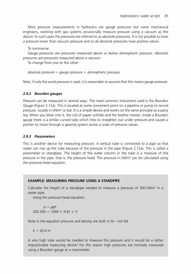
Most pressure measurements in hydraulics are gauge pressures but some mechanicalengineers, working with gas systems occasionally measure pressure using a vacuum as thedatum. In such cases the pressures are referred to as absolute pressures. It is not possible to havea pressure lower than vacuum pressure and so all absolute pressures have positive values.
To summarise:Gauge pressures are pressures measured above or below atmospheric pressure. Absolute
pressures are pressures measured above a vacuum.To change from one to the other:
absolute pressure � gauge pressure � atmospheric pressure
Note, if only the word pressure is used, it is reasonable to assume that this means gauge pressure.
2.9.2 Bourdon gauges
Pressure can be measured in several ways. The most common instrument used is the BourdonGauge (Figure 2.12a). This is located at some convenient point on a pipeline or pump to recordpressure, usually in kN/m2 or bar. It is a simple device and works on the same principle as a partytoy. When you blow into it, the coil of paper unfolds and the feather rotates. Inside a Bourdongauge there is a similar curved tube which tries to straighten out under pressure and causes apointer to move through a gearing system across a scale of pressure values.
2.9.3 Piezometers
This is another device for measuring pressure. A vertical tube is connected to a pipe so thatwater can rise up the tube because of the pressure in the pipe (Figure 2.12a). This is called apiezometer or standpipe. The height of the water column in the tube is a measure of thepressure in the pipe, that is, the pressure head. The pressure in kN/m2 can be calculated usingthe pressure-head equation.
Hydrostatics: water at rest 35
EXAMPLE: MEASURING PRESSURE USING A STANDPIPE
Calculate the height of a standpipe needed to measure a pressure of 200 kN/m2 in awater pipe.
Using the pressure-head equation:
p � �gh200 000 � 1000 � 9.81 � h
Note in the equation pressure and density are both in N – not kN.
h � 20.4 m
A very high tube would be needed to measure this pressure and it would be a ratherimpracticable measuring device! For this reason high pressures are normally measuredusing a Bourdon gauge or a manometer.
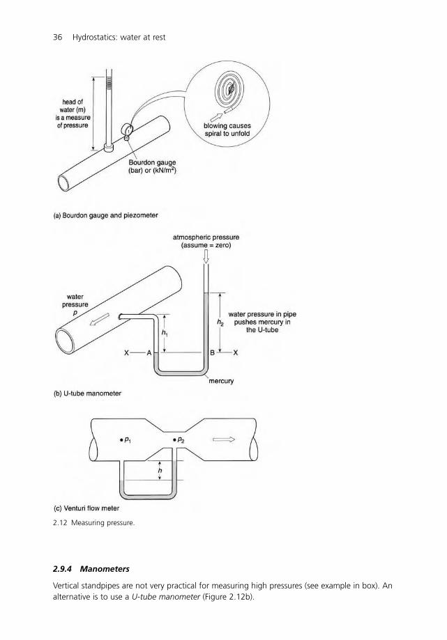
36 Hydrostatics: water at rest
2.9.4 Manometers
Vertical standpipes are not very practical for measuring high pressures (see example in box). Analternative is to use a U-tube manometer (Figure 2.12b).
2.12 Measuring pressure.
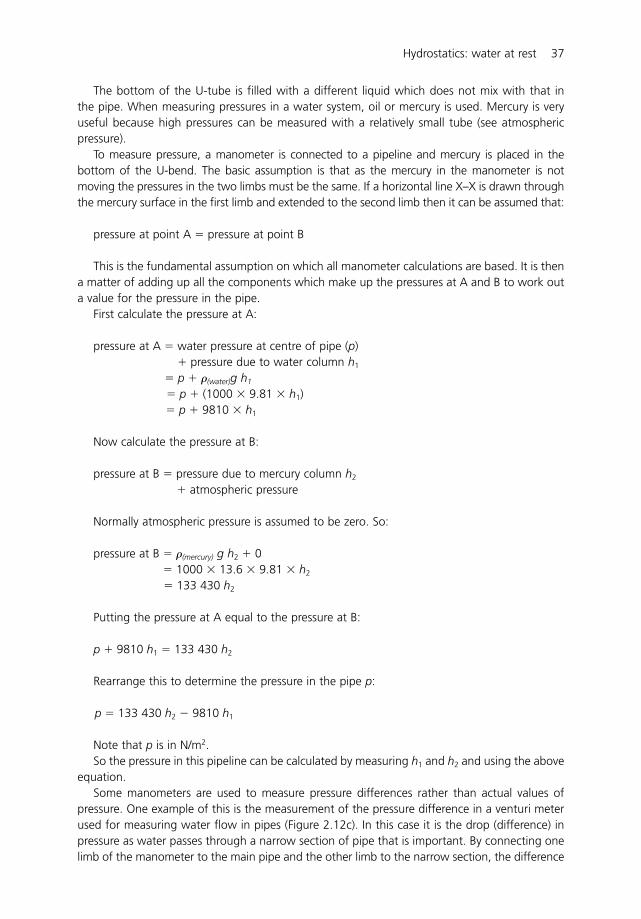
The bottom of the U-tube is filled with a different liquid which does not mix with that inthe pipe. When measuring pressures in a water system, oil or mercury is used. Mercury is veryuseful because high pressures can be measured with a relatively small tube (see atmosphericpressure).
To measure pressure, a manometer is connected to a pipeline and mercury is placed in thebottom of the U-bend. The basic assumption is that as the mercury in the manometer is notmoving the pressures in the two limbs must be the same. If a horizontal line X–X is drawn throughthe mercury surface in the first limb and extended to the second limb then it can be assumed that:
pressure at point A � pressure at point B
This is the fundamental assumption on which all manometer calculations are based. It is thena matter of adding up all the components which make up the pressures at A and B to work outa value for the pressure in the pipe.
First calculate the pressure at A:
pressure at A � water pressure at centre of pipe (p)� pressure due to water column h1
� p � �(water)g h1
� p � (1000 � 9.81 � h1)� p � 9810 � h1
Now calculate the pressure at B:
pressure at B � pressure due to mercury column h2
� atmospheric pressure
Normally atmospheric pressure is assumed to be zero. So:
pressure at B � �(mercury) g h2 � 0� 1000 � 13.6 � 9.81 � h2
� 133 430 h2
Putting the pressure at A equal to the pressure at B:
p � 9810 h1 � 133 430 h2
Rearrange this to determine the pressure in the pipe p:
p � 133 430 h2 � 9810 h1
Note that p is in N/m2.So the pressure in this pipeline can be calculated by measuring h1 and h2 and using the above
equation.Some manometers are used to measure pressure differences rather than actual values of
pressure. One example of this is the measurement of the pressure difference in a venturi meterused for measuring water flow in pipes (Figure 2.12c). In this case it is the drop (difference) inpressure as water passes through a narrow section of pipe that is important. By connecting onelimb of the manometer to the main pipe and the other limb to the narrow section, the difference
Hydrostatics: water at rest 37
38 Hydrostatics: water at rest
EXAMPLE: MEASURING PRESSURE USING A MANOMETER
A mercury manometer is used to measure the pressure in a water pipe (Figure 2.12c).Calculate the pressure in the pipe when h1 � 1.5 m and h2 � 0.8 m.
To solve this problem start with the principle on which all manometers are based:
pressure at A � pressure at B
Calculate the pressures at A and B:
pressure at A � water pressure in pipe (p)� pressure due to water column h1
� p � �(water)g h1
� p � 1000 � 9.81 � 1.5pressure at B � pressure due to mercury column h2
� atmospheric pressure� �(mercury)g h2 � 0� 1000 � 13.6 � 9.81 � 0.8
Note that as all the pressures are gauge pressures, atmospheric pressure is assumed tobe zero.
Putting the pressure at A equal to the pressure at B:
p � 1000 � 9.81 � 1.5 � 1000 � 13.6 � 9.81 � 0.8
Rearrange this to determine p:
p � (1000 � 13.6 � 9.81 � 0.8) � (1000 � 9.81 � 1.5)� 106 732 � 14 715� 92 017 N/m2
p � 92 kN/m2
in pressure can be determined. Note that the pressure difference is not just the difference inthe mercury readings on the two columns as is often thought. The pressure difference must becalculated using the principle described above for the simple manometer. More about venturemeters and using manometers in Section 4.10.
The best way to deal with manometer measurements is to remember the principle on whichall manometer calculations are based and not the formula for p. There are many different waysof arranging manometers with different fluids in them and so there will be too many formulaeto remember. So just remember and apply the principle – pressure on each side of themanometer is the same across a horizontal line AB – then the pressure can be easily determined.See the worked example in the box.
2.10 Designing dams
Engineers are always interested in the ways in which things fall down or collapse so they candevise design and construction procedures that produce safe reliable structures. Dams in
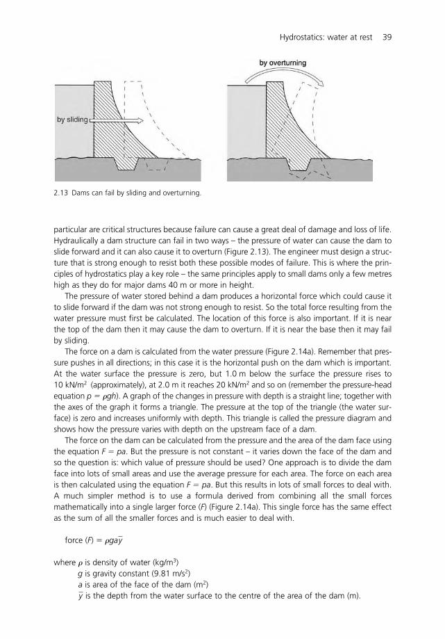
particular are critical structures because failure can cause a great deal of damage and loss of life.Hydraulically a dam structure can fail in two ways – the pressure of water can cause the dam toslide forward and it can also cause it to overturn (Figure 2.13). The engineer must design a struc-ture that is strong enough to resist both these possible modes of failure. This is where the prin-ciples of hydrostatics play a key role – the same principles apply to small dams only a few metreshigh as they do for major dams 40 m or more in height.
The pressure of water stored behind a dam produces a horizontal force which could cause itto slide forward if the dam was not strong enough to resist. So the total force resulting from thewater pressure must first be calculated. The location of this force is also important. If it is nearthe top of the dam then it may cause the dam to overturn. If it is near the base then it may failby sliding.
The force on a dam is calculated from the water pressure (Figure 2.14a). Remember that pres-sure pushes in all directions; in this case it is the horizontal push on the dam which is important.At the water surface the pressure is zero, but 1.0 m below the surface the pressure rises to10 kN/m2 (approximately), at 2.0 m it reaches 20 kN/m2 and so on (remember the pressure-headequation p � �gh). A graph of the changes in pressure with depth is a straight line; together withthe axes of the graph it forms a triangle. The pressure at the top of the triangle (the water sur-face) is zero and increases uniformly with depth. This triangle is called the pressure diagram andshows how the pressure varies with depth on the upstream face of a dam.
The force on the dam can be calculated from the pressure and the area of the dam face usingthe equation F � pa. But the pressure is not constant – it varies down the face of the dam andso the question is: which value of pressure should be used? One approach is to divide the damface into lots of small areas and use the average pressure for each area. The force on each areais then calculated using the equation F � pa. But this results in lots of small forces to deal with.A much simpler method is to use a formula derived from combining all the small forcesmathematically into a single larger force (F) (Figure 2.14a). This single force has the same effectas the sum of all the smaller forces and is much easier to deal with.
force (F) � �ga
where � is density of water (kg/m3)g is gravity constant (9.81 m/s2)a is area of the face of the dam (m2)
is the depth from the water surface to the centre of the area of the dam (m).y
y
Hydrostatics: water at rest 39
2.13 Dams can fail by sliding and overturning.
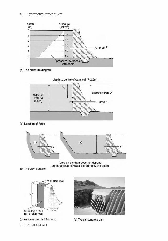
40 Hydrostatics: water at rest
2.14 Designing a dam.
Hydrostatics: water at rest 41
EXAMPLE: CALCULATING THE FORCE ON A DAM
A farm dam is to be constructed to contain water up to 5 m deep. Calculate the force onthe dam and the position of the force in relation to the water surface (Figure 2.14b).Calculate the force F:
F � �ga
where � � 1000 kg/m3, g � 9.81 m/s2 and a � b � h � 1 � 5 � 5 m.Note: when the length of the dam is not given assume that b � 1 m. The force is thenthe force per metre length of the dam (Figure 2.14d).
Put all these values into the formula for F:
F � 1000 � 9.81 � 5 � 2.5� 122 625 N
F � 122.6 kNm length of the dam
Using the alternative method of calculating the area of the pressure diagram:
area of pressure diagram (triangle) �12
� base � height
y � h2
� 2.5 m
y
For the mathematically minded, a derivation of this formula can be found in most engineeringhydraulics text books.
Returning to the pressure diagram, this can also be used to determine the resultant force. Itis in fact equal to the area of the diagram, that is, the area of the triangle. To see how this,and the formula for force, works look at the example of how to calculate the force on a dam inthe box.
The position of this force is also important. To determine the depth D from the water surfaceto the resultant force F (Figure 2.14b) on the dam the following formula can be used:
where h is height of the dam face in contact with the water (m) and is the depth from thewater surface to the centre of the area of the dam (m).
As with the force formula, this one can also be derived from the principles of hydrostatics.The pressure diagram can also be used to determine D. The force is located at the centre ofthe diagram; as this is a triangle it is located two-thirds down from the apex (i.e. from the watersurface).
Note that these formulae only work for simple vertical dams. When more complex shapes areinvolved, such as earth dams with sloping sides, then the formulae do not work. But solving theproblem is not so difficult – it relies on applying the same hydrostatic principles. Most standardcivil engineering texts will show you how.
y
D �
h2
12y�y
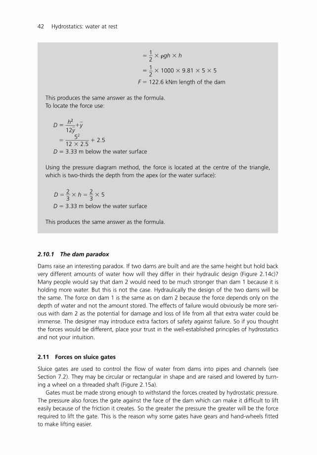
2.10.1 The dam paradox
Dams raise an interesting paradox. If two dams are built and are the same height but hold backvery different amounts of water how will they differ in their hydraulic design (Figure 2.14c)?Many people would say that dam 2 would need to be much stronger than dam 1 because it isholding more water. But this is not the case. Hydraulically the design of the two dams will bethe same. The force on dam 1 is the same as on dam 2 because the force depends only on thedepth of water and not the amount stored. The effects of failure would obviously be more seri-ous with dam 2 as the potential for damage and loss of life from all that extra water could beimmense. The designer may introduce extra factors of safety against failure. So if you thoughtthe forces would be different, place your trust in the well-established principles of hydrostaticsand not your intuition.
2.11 Forces on sluice gates
Sluice gates are used to control the flow of water from dams into pipes and channels (seeSection 7.2). They may be circular or rectangular in shape and are raised and lowered by turn-ing a wheel on a threaded shaft (Figure 2.15a).
Gates must be made strong enough to withstand the forces created by hydrostatic pressure.The pressure also forces the gate against the face of the dam which can make it difficult to lifteasily because of the friction it creates. So the greater the pressure the greater will be the forcerequired to lift the gate. This is the reason why some gates have gears and hand-wheels fittedto make lifting easier.
42 Hydrostatics: water at rest
�
�
F � 122.6 kNm length of the dam
This produces the same answer as the formula.To locate the force use:
D �
�
D � 3.33 m below the water surface
Using the pressure diagram method, the force is located at the centre of the triangle,which is two-thirds the depth from the apex (or the water surface):
D �
D � 3.33 m below the water surface
This produces the same answer as the formula.
23
� h � 23
� 5
52
12 � 2.5 � 2.5
h2
12y�y
12
� 1000 � 9.81 � 5 � 5
12
� gh � h
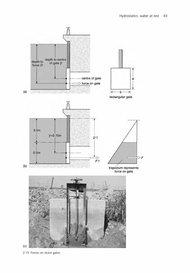
Hydrostatics: water at rest 43
2.15 Forces on sluice gates.
(c)
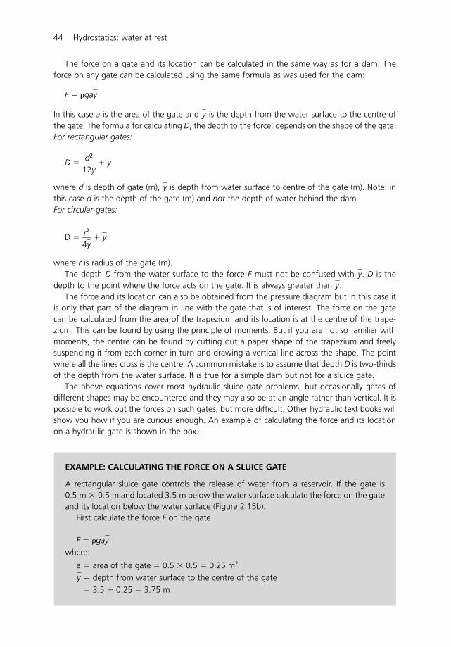
The force on a gate and its location can be calculated in the same way as for a dam. Theforce on any gate can be calculated using the same formula as was used for the dam:
In this case a is the area of the gate and is the depth from the water surface to the centre ofthe gate. The formula for calculating D, the depth to the force, depends on the shape of the gate.For rectangular gates:
where d is depth of gate (m), is depth from water surface to centre of the gate (m). Note: inthis case d is the depth of the gate (m) and not the depth of water behind the dam.For circular gates:
where r is radius of the gate (m).The depth D from the water surface to the force F must not be confused with . D is the
depth to the point where the force acts on the gate. It is always greater than .The force and its location can also be obtained from the pressure diagram but in this case it
is only that part of the diagram in line with the gate that is of interest. The force on the gatecan be calculated from the area of the trapezium and its location is at the centre of the trape-zium. This can be found by using the principle of moments. But if you are not so familiar withmoments, the centre can be found by cutting out a paper shape of the trapezium and freelysuspending it from each corner in turn and drawing a vertical line across the shape. The pointwhere all the lines cross is the centre. A common mistake is to assume that depth D is two-thirdsof the depth from the water surface. It is true for a simple dam but not for a sluice gate.
The above equations cover most hydraulic sluice gate problems, but occasionally gates ofdifferent shapes may be encountered and they may also be at an angle rather than vertical. It ispossible to work out the forces on such gates, but more difficult. Other hydraulic text books willshow you how if you are curious enough. An example of calculating the force and its locationon a hydraulic gate is shown in the box.
yy
D � r2
4y � y
y
D � d2
12y � y
y
F � gay
44 Hydrostatics: water at rest
EXAMPLE: CALCULATING THE FORCE ON A SLUICE GATE
A rectangular sluice gate controls the release of water from a reservoir. If the gate is0.5 m � 0.5 m and located 3.5 m below the water surface calculate the force on the gateand its location below the water surface (Figure 2.15b).
First calculate the force F on the gate
where:
a � area of the gate � 0.5 � 0.5 � 0.25 m2
� depth from water surface to the centre of the gate� 3.5 � 0.25 � 3.75 m
y
F � gay
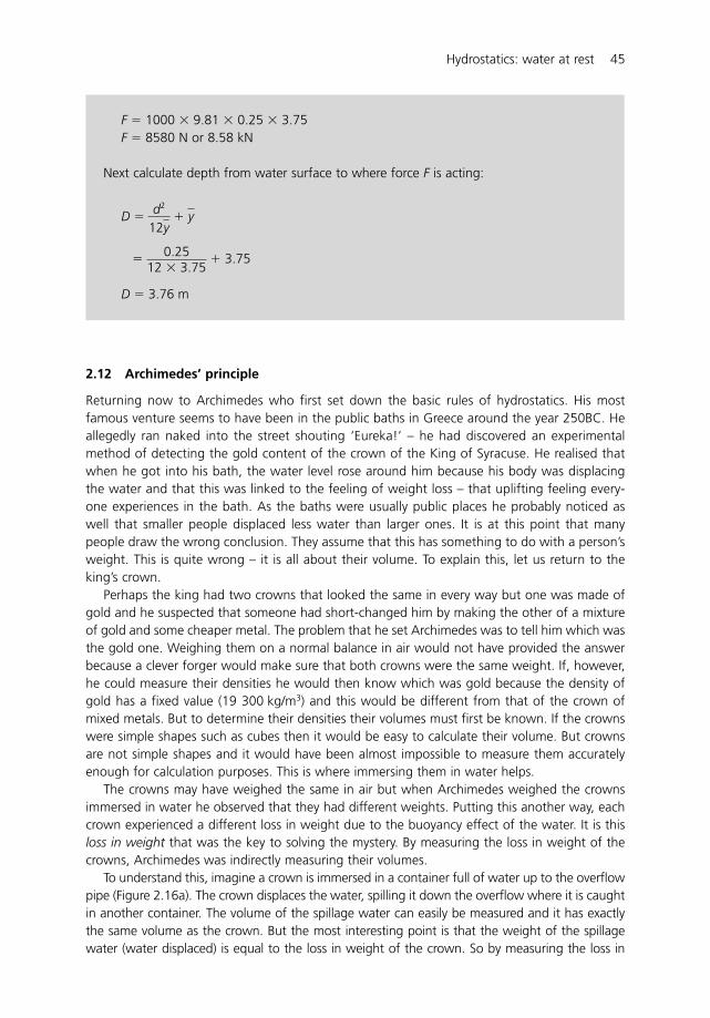
2.12 Archimedes’ principle
Returning now to Archimedes who first set down the basic rules of hydrostatics. His mostfamous venture seems to have been in the public baths in Greece around the year 250BC. Heallegedly ran naked into the street shouting ‘Eureka!’ – he had discovered an experimentalmethod of detecting the gold content of the crown of the King of Syracuse. He realised thatwhen he got into his bath, the water level rose around him because his body was displacingthe water and that this was linked to the feeling of weight loss – that uplifting feeling every-one experiences in the bath. As the baths were usually public places he probably noticed aswell that smaller people displaced less water than larger ones. It is at this point that manypeople draw the wrong conclusion. They assume that this has something to do with a person’sweight. This is quite wrong – it is all about their volume. To explain this, let us return to theking’s crown.
Perhaps the king had two crowns that looked the same in every way but one was made ofgold and he suspected that someone had short-changed him by making the other of a mixtureof gold and some cheaper metal. The problem that he set Archimedes was to tell him which wasthe gold one. Weighing them on a normal balance in air would not have provided the answerbecause a clever forger would make sure that both crowns were the same weight. If, however,he could measure their densities he would then know which was gold because the density ofgold has a fixed value (19 300 kg/m3) and this would be different from that of the crown ofmixed metals. But to determine their densities their volumes must first be known. If the crownswere simple shapes such as cubes then it would be easy to calculate their volume. But crownsare not simple shapes and it would have been almost impossible to measure them accuratelyenough for calculation purposes. This is where immersing them in water helps.
The crowns may have weighed the same in air but when Archimedes weighed the crownsimmersed in water he observed that they had different weights. Putting this another way, eachcrown experienced a different loss in weight due to the buoyancy effect of the water. It is thisloss in weight that was the key to solving the mystery. By measuring the loss in weight of thecrowns, Archimedes was indirectly measuring their volumes.
To understand this, imagine a crown is immersed in a container full of water up to the overflowpipe (Figure 2.16a). The crown displaces the water, spilling it down the overflow where it is caughtin another container. The volume of the spillage water can easily be measured and it has exactlythe same volume as the crown. But the most interesting point is that the weight of the spillagewater (water displaced) is equal to the loss in weight of the crown. So by measuring the loss in
Hydrostatics: water at rest 45
F � 1000 � 9.81 � 0.25 � 3.75F � 8580 N or 8.58 kN
Next calculate depth from water surface to where force F is acting:
D �
�
D � 3.76 m
0.2512 � 3.75
� 3.75
d2
12y � y
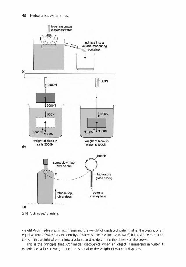
46 Hydrostatics: water at rest
2.16 Archimedes’ principle.
weight Archimedes was in fact measuring the weight of displaced water, that is, the weight of anequal volume of water. As the density of water is a fixed value (9810 N/m3) it is a simple matter toconvert this weight of water into a volume and so determine the density of the crown.
This is the principle that Archimedes discovered: when an object is immersed in water itexperiences a loss in weight and this is equal to the weight of water it displaces.
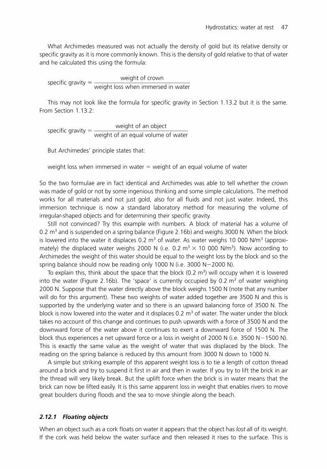
What Archimedes measured was not actually the density of gold but its relative density orspecific gravity as it is more commonly known. This is the density of gold relative to that of waterand he calculated this using the formula:
This may not look like the formula for specific gravity in Section 1.13.2 but it is the same.From Section 1.13.2:
But Archimedes’ principle states that:
weight loss when immersed in water � weight of an equal volume of water
So the two formulae are in fact identical and Archimedes was able to tell whether the crownwas made of gold or not by some ingenious thinking and some simple calculations. The methodworks for all materials and not just gold, also for all fluids and not just water. Indeed, thisimmersion technique is now a standard laboratory method for measuring the volume ofirregular-shaped objects and for determining their specific gravity.
Still not convinced? Try this example with numbers. A block of material has a volume of0.2 m3 and is suspended on a spring balance (Figure 2.16b) and weighs 3000 N. When the blockis lowered into the water it displaces 0.2 m3 of water. As water weighs 10 000 N/m3 (approxi-mately) the displaced water weighs 2000 N (i.e. 0.2 m3 � 10 000 N/m3). Now according toArchimedes the weight of this water should be equal to the weight loss by the block and so thespring balance should now be reading only 1000 N (i.e. 3000 N�2000 N).
To explain this, think about the space that the block (0.2 m3) will occupy when it is loweredinto the water (Figure 2.16b). The ‘space’ is currently occupied by 0.2 m3 of water weighing2000 N. Suppose that the water directly above the block weighs 1500 N (note that any numberwill do for this argument). These two weights of water added together are 3500 N and this issupported by the underlying water and so there is an upward balancing force of 3500 N. Theblock is now lowered into the water and it displaces 0.2 m3 of water. The water under the blocktakes no account of this change and continues to push upwards with a force of 3500 N and thedownward force of the water above it continues to exert a downward force of 1500 N. Theblock thus experiences a net upward force or a loss in weight of 2000 N (i.e. 3500 N�1500 N).This is exactly the same value as the weight of water that was displaced by the block. Thereading on the spring balance is reduced by this amount from 3000 N down to 1000 N.
A simple but striking example of this apparent weight loss is to tie a length of cotton threadaround a brick and try to suspend it first in air and then in water. If you try to lift the brick in airthe thread will very likely break. But the uplift force when the brick is in water means that thebrick can now be lifted easily. It is this same apparent loss in weight that enables rivers to movegreat boulders during floods and the sea to move shingle along the beach.
2.12.1 Floating objects
When an object such as a cork floats on water it appears that the object has lost all of its weight.If the cork was held below the water surface and then released it rises to the surface. This is
specific gravity � weight of an object
weight of an equal volume of water
specific gravity � weight of crown
weight loss when immersed in water
Hydrostatics: water at rest 47
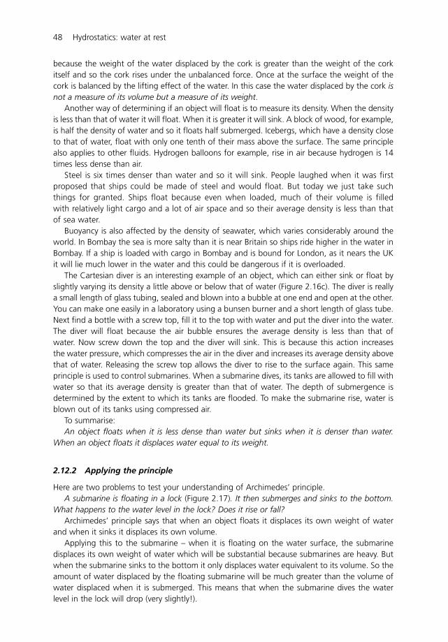
because the weight of the water displaced by the cork is greater than the weight of the corkitself and so the cork rises under the unbalanced force. Once at the surface the weight of thecork is balanced by the lifting effect of the water. In this case the water displaced by the cork isnot a measure of its volume but a measure of its weight.
Another way of determining if an object will float is to measure its density. When the densityis less than that of water it will float. When it is greater it will sink. A block of wood, for example,is half the density of water and so it floats half submerged. Icebergs, which have a density closeto that of water, float with only one tenth of their mass above the surface. The same principlealso applies to other fluids. Hydrogen balloons for example, rise in air because hydrogen is 14times less dense than air.
Steel is six times denser than water and so it will sink. People laughed when it was firstproposed that ships could be made of steel and would float. But today we just take suchthings for granted. Ships float because even when loaded, much of their volume is filledwith relatively light cargo and a lot of air space and so their average density is less than thatof sea water.
Buoyancy is also affected by the density of seawater, which varies considerably around theworld. In Bombay the sea is more salty than it is near Britain so ships ride higher in the water inBombay. If a ship is loaded with cargo in Bombay and is bound for London, as it nears the UKit will lie much lower in the water and this could be dangerous if it is overloaded.
The Cartesian diver is an interesting example of an object, which can either sink or float byslightly varying its density a little above or below that of water (Figure 2.16c). The diver is reallya small length of glass tubing, sealed and blown into a bubble at one end and open at the other.You can make one easily in a laboratory using a bunsen burner and a short length of glass tube.Next find a bottle with a screw top, fill it to the top with water and put the diver into the water.The diver will float because the air bubble ensures the average density is less than that ofwater. Now screw down the top and the diver will sink. This is because this action increasesthe water pressure, which compresses the air in the diver and increases its average density abovethat of water. Releasing the screw top allows the diver to rise to the surface again. This sameprinciple is used to control submarines. When a submarine dives, its tanks are allowed to fill withwater so that its average density is greater than that of water. The depth of submergence isdetermined by the extent to which its tanks are flooded. To make the submarine rise, water isblown out of its tanks using compressed air.
To summarise:An object floats when it is less dense than water but sinks when it is denser than water.
When an object floats it displaces water equal to its weight.
2.12.2 Applying the principle
Here are two problems to test your understanding of Archimedes’ principle.A submarine is floating in a lock (Figure 2.17). It then submerges and sinks to the bottom.
What happens to the water level in the lock? Does it rise or fall?Archimedes’ principle says that when an object floats it displaces its own weight of water
and when it sinks it displaces its own volume.Applying this to the submarine – when it is floating on the water surface, the submarine
displaces its own weight of water which will be substantial because submarines are heavy. Butwhen the submarine sinks to the bottom it only displaces water equivalent to its volume. So theamount of water displaced by the floating submarine will be much greater than the volume ofwater displaced when it is submerged. This means that when the submarine dives the waterlevel in the lock will drop (very slightly!).
48 Hydrostatics: water at rest
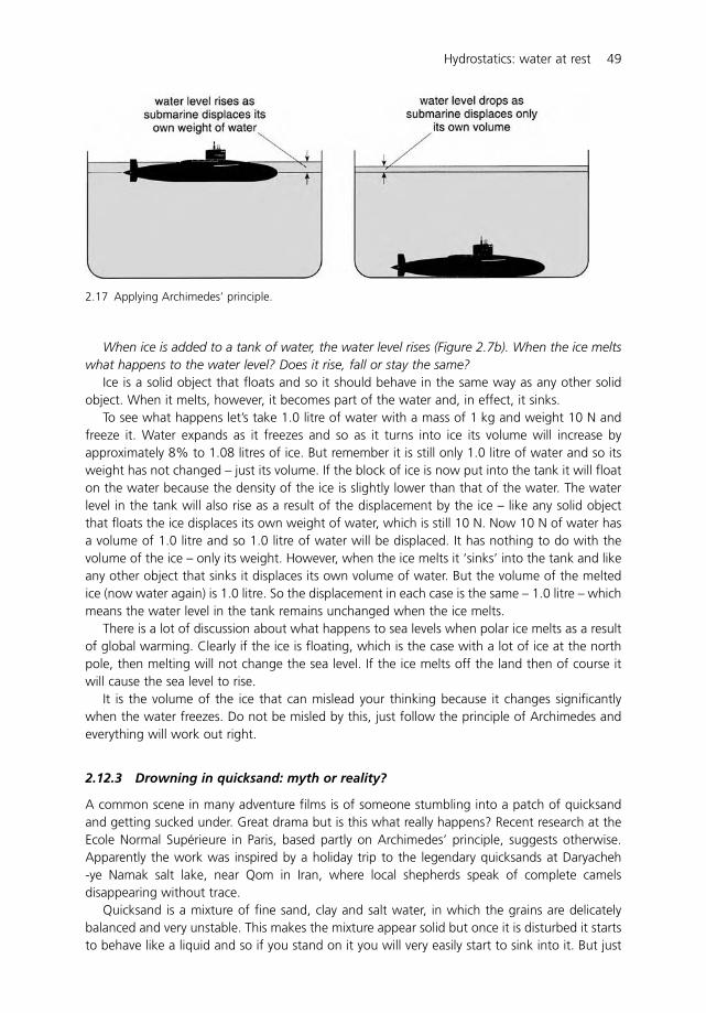
When ice is added to a tank of water, the water level rises (Figure 2.7b). When the ice meltswhat happens to the water level? Does it rise, fall or stay the same?
Ice is a solid object that floats and so it should behave in the same way as any other solidobject. When it melts, however, it becomes part of the water and, in effect, it sinks.
To see what happens let’s take 1.0 litre of water with a mass of 1 kg and weight 10 N andfreeze it. Water expands as it freezes and so as it turns into ice its volume will increase byapproximately 8% to 1.08 litres of ice. But remember it is still only 1.0 litre of water and so itsweight has not changed – just its volume. If the block of ice is now put into the tank it will floaton the water because the density of the ice is slightly lower than that of the water. The waterlevel in the tank will also rise as a result of the displacement by the ice – like any solid objectthat floats the ice displaces its own weight of water, which is still 10 N. Now 10 N of water hasa volume of 1.0 litre and so 1.0 litre of water will be displaced. It has nothing to do with thevolume of the ice – only its weight. However, when the ice melts it ‘sinks’ into the tank and likeany other object that sinks it displaces its own volume of water. But the volume of the meltedice (now water again) is 1.0 litre. So the displacement in each case is the same – 1.0 litre – whichmeans the water level in the tank remains unchanged when the ice melts.
There is a lot of discussion about what happens to sea levels when polar ice melts as a resultof global warming. Clearly if the ice is floating, which is the case with a lot of ice at the northpole, then melting will not change the sea level. If the ice melts off the land then of course itwill cause the sea level to rise.
It is the volume of the ice that can mislead your thinking because it changes significantlywhen the water freezes. Do not be misled by this, just follow the principle of Archimedes andeverything will work out right.
2.12.3 Drowning in quicksand: myth or reality?
A common scene in many adventure films is of someone stumbling into a patch of quicksandand getting sucked under. Great drama but is this what really happens? Recent research at theEcole Normal Supérieure in Paris, based partly on Archimedes’ principle, suggests otherwise.Apparently the work was inspired by a holiday trip to the legendary quicksands at Daryacheh-ye Namak salt lake, near Qom in Iran, where local shepherds speak of complete camelsdisappearing without trace.
Quicksand is a mixture of fine sand, clay and salt water, in which the grains are delicatelybalanced and very unstable. This makes the mixture appear solid but once it is disturbed it startsto behave like a liquid and so if you stand on it you will very easily start to sink into it. But just
Hydrostatics: water at rest 49
2.17 Applying Archimedes’ principle.
like any liquid there is a buoyancy effect (Archimedes’ principle) and so how far you will sinkdepends on your density. So if you float in water you will also float in quicksand.
But the problem is not just a hydraulic one. The research showed that when the mixtureliquefies the sand and clay fall to the bottom and create thick sediment that also helps toprevent you sinking further. So the good news is that the two combined mean that you areunlikely to sink much beyond your waist – not such good news if you fell in head first. Strugglingand kicking will not make you sink further – it just makes the mixture more unstable and so youwill sink faster. The bad news comes when you try to get out because the mixture will hold youfast. It can take as much force to pull you out of quicksand as it does to lift a typical family car.So you are more likely to have your limbs pulled off than get out of the mess! So how do youget out? One suggestion by the researchers is to gently wriggle your feet to liquefy the mixtureand then slowly pull yourself up a few millimetres at a time. The myth surrounding quicksandprobably originates from people falling in head first and in such circumstances you are mostlikely to drown. Science also spoils a good story – it means that all those film dramas aboutquicksand such as The Hound of the Baskervilles are pure fantasy!
2.13 Some examples to test your understanding
1 Determine the pressure in kN/m2 for a head of a) 14 m of water and b) 1.7 m of oil. Assumethe mass density of water is 1000 kg/m3 and oil is 785 kg/m3 (137.34 kN/m2, 13.09 kN/m2).
2 A storage tank, 2.3 m long by 1.2 m wide and 0.8 m deep is full of water. Calculate (a)the mass of water in the tank, (b) the pressure on the bottom of the tank, (c) the force onthe end of the tank and (d) the position of this force below the water surface (2210 kg,7848 N/m2, 3767 N, 0.53 m below the water surface).
3 Calculate atmospheric pressure in kN/m2 when the barometer reading is 750 mm ofmercury. Calculate the height of a water barometer needed to measure atmosphericpressure (100.06 kN/m2, 10.2 m).
4 Calculate the pressure in kN/m2 and in m head of water in a pipeline carrying water usinga mercury manometer when h1 � 0.5 m and h2 � 1.2 m. Assume the specific gravity ofmercury is 13.6 (155 kN/m2, 15.82 m).
5 A vertical rectangular sluice gate 1.0 m high by 0.5 m wide is used to control the dischargefrom a storage reservoir. Calculate the horizontal force on the gate and it location inrelation to the water surface when the top of the gate is located 2.3 m below the watersurface (13.73 kN, 2.83 m).
6 Calculate the force and its location below the water surface on a 0.75 m diameter circularsluice gate located when the top of the gate is located 2.3 m below the water surface(11.57 kN, 2.69 m).
50 Hydrostatics: water at rest
3 Hydrodynamics: when water starts to flow
3.1 Introduction
Hydrodynamics is the study of water flow. It helps us to understand how water behaves whenit flows in pipes and channels and to answer such questions as – what diameter of pipe isneeded to supply a village or a town with water? How wide and deep must a channel be tocarry water from a dam to an irrigation scheme? What kind of pumps may be required and howbig must they be? These are the practical problems of hydrodynamics.
Hydrodynamics is more complex than hydrostatics because it must take account of morefactors, particularly the direction and velocity in which the water is flowing and the influence ofviscosity. In early times hydrodynamics, like many other developments, moved forward on a trialand error basis. If the flow was not enough then a larger diameter pipe was used, if a pipe burstunder the water pressure then a stronger one was put in its place. But during the past 250 yearsor so scientists have found new ways of answering the questions about size, shape and strength.They experimented in laboratories and came up with mathematical theories that have nowreplaced trial and error methods for the most common hydraulic problems.
3.2 Experimentation and theory
Experimentation was a logical next step from trial and error. Scientists built physical models ofhydraulic systems in the laboratory and tested them before building the real thing. Much of ourcurrent knowledge of water flow in pipes and open channels has come from this kind of exper-imentation; empirical formulae were derived from the data collected to link water flow with thesize of pipes and channels. Today we use formulae for most design problems, but there are stillsome problems which are not easily solved in this way. Practical laboratory experiments are stillused to find solutions for the design of complex works such as harbours, tidal power stations,river flood control schemes and dam spillways. Small-scale models are built to test new designsand to investigate the impact of new engineering works both locally and in the surrounding area(Figure 3.1).
Formulae that link water flow with pipe and channel sizes have also been developedanalytically from our understanding of the basic principles of physics – the properties of water andNewton’s laws of motion. The rules of hydrostatics were developed analytically and have provedto work very well. But when water starts to move it is difficult to take account of all the newfactors involved, in particular viscosity. The engineering approach, rather than the scientific one,
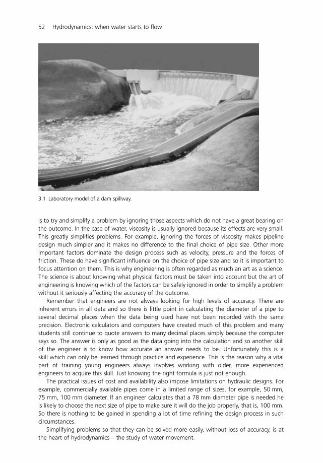
is to try and simplify a problem by ignoring those aspects which do not have a great bearing onthe outcome. In the case of water, viscosity is usually ignored because its effects are very small.This greatly simplifies problems. For example, ignoring the forces of viscosity makes pipelinedesign much simpler and it makes no difference to the final choice of pipe size. Other moreimportant factors dominate the design process such as velocity, pressure and the forces offriction. These do have significant influence on the choice of pipe size and so it is important tofocus attention on them. This is why engineering is often regarded as much an art as a science.The science is about knowing what physical factors must be taken into account but the art ofengineering is knowing which of the factors can be safely ignored in order to simplify a problemwithout it seriously affecting the accuracy of the outcome.
Remember that engineers are not always looking for high levels of accuracy. There areinherent errors in all data and so there is little point in calculating the diameter of a pipe toseveral decimal places when the data being used have not been recorded with the sameprecision. Electronic calculators and computers have created much of this problem and manystudents still continue to quote answers to many decimal places simply because the computersays so. The answer is only as good as the data going into the calculation and so another skillof the engineer is to know how accurate an answer needs to be. Unfortunately this is askill which can only be learned through practice and experience. This is the reason why a vitalpart of training young engineers always involves working with older, more experiencedengineers to acquire this skill. Just knowing the right formula is just not enough.
The practical issues of cost and availability also impose limitations on hydraulic designs. Forexample, commercially available pipes come in a limited range of sizes, for example, 50 mm,75 mm, 100 mm diameter. If an engineer calculates that a 78 mm diameter pipe is needed heis likely to choose the next size of pipe to make sure it will do the job properly, that is, 100 mm.So there is nothing to be gained in spending a lot of time refining the design process in suchcircumstances.
Simplifying problems so that they can be solved more easily, without loss of accuracy, is atthe heart of hydrodynamics – the study of water movement.
52 Hydrodynamics: when water starts to flow
3.1 Laboratory model of a dam spillway.
3.3 Hydraulic toolbox
The development of hydraulic theory has produced three important basic tools (equations)which are fundamental to solving most hydrodynamic problems:
� discharge and continuity� energy� momentum.
They are not difficult to master and you will need to understand them well.
3.4 Discharge and continuity
Discharge refers to the volume of water flowing along a pipe or channel each second. Volumeis measured in cubic metres (m3) and so discharge is measured in cubic metres per second (m3/s).Alternative units are litres per second (l/s) and cubic metres per hour (m3/h).
There are two ways of determining discharge. The first involves measuring the volume ofwater flowing in a system over a given time period. For example, water flowing from a pipe canbe caught in a bucket of known volume (Figure 3.2a). If the time to fill the bucket is recordedthen the discharge from the pipe can be determined using the following formula:
discharge (m3/s)
Discharge can also be determined by multiplying the velocity of the water by the area of theflow. To understand this, imagine water flowing along a pipeline (Figure 3.2b). In one secondthe volume of water flowing past �–� will be the shaded volume. This volume can becalculated by multiplying the area of the pipe by the length of the shaded portion. But theshaded length is numerically equal to the velocity v and so the volume flowing each second (i.e.the discharge) is equal to the pipe area multiplied by the velocity. Writing this as an equation:
discharge (Q) � velocity (v) � area (a)Q � va
The continuity equation builds on the discharge equation and simply means that the amount ofwater flowing into a system must be equal to the amount of water flowing out of it (Figure 3.2c).
inflow � outflow
And so:
Q1 � Q2
But from the discharge equation:
Q � va
And so:
v1a1 � v2a2
So the continuity equation not only links discharges it also links areas and velocities as well. Thisis a very simple but powerful equation and is fundamental to solving many hydraulic problems. Anexample in the box shows how this works in practice for a pipeline which changes diameter.
� volume (m3)
time (s)
Hydrodynamics: when water starts to flow 53
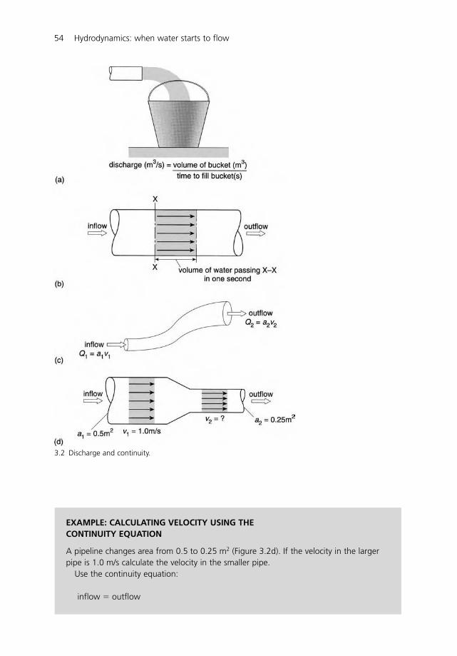
54 Hydrodynamics: when water starts to flow
3.2 Discharge and continuity.
EXAMPLE: CALCULATING VELOCITY USING THE CONTINUITY EQUATION
A pipeline changes area from 0.5 to 0.25 m2 (Figure 3.2d). If the velocity in the largerpipe is 1.0 m/s calculate the velocity in the smaller pipe.
Use the continuity equation:
inflow � outflow
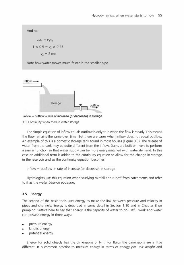
The simple equation of inflow equals outflow is only true when the flow is steady. This meansthe flow remains the same over time. But there are cases when inflow does not equal outflow.An example of this is a domestic storage tank found in most houses (Figure 3.3). The release ofwater from the tank may be quite different from the inflow. Dams are built on rivers to performa similar function so that water supply can be more easily matched with water demand. In thiscase an additional term is added to the continuity equation to allow for the change in storagein the reservoir and so the continuity equation becomes:
inflow � outflow � rate of increase (or decrease) in storage
Hydrologists use this equation when studying rainfall and runoff from catchments and referto it as the water balance equation.
3.5 Energy
The second of the basic tools uses energy to make the link between pressure and velocity inpipes and channels. Energy is described in some detail in Section 1.10 and in Chapter 8 onpumping. Suffice here to say that energy is the capacity of water to do useful work and watercan possess energy in three ways:
� pressure energy� kinetic energy� potential energy.
Energy for solid objects has the dimensions of Nm. For fluids the dimensions are a littledifferent. It is common practice to measure energy in terms of energy per unit weight and
Hydrodynamics: when water starts to flow 55
And so:
v1a1 � v2a2
1 � 0.5 � v2 � 0.25
v2 � 2 m/s
Note how water moves much faster in the smaller pipe.
3.3 Continuity when there is water storage.

so energy for fluids has dimensions of Nm/N. The Newton terms cancel each other out and weare left with metres (m). This make energy look similar to pressure head as both are measured inmetres. Indeed we shall see that the terms energy and pressure head are in fact interchangeable.
So let’s explore these three types of energy.
3.5.1 Pressure energy
When water is under pressure it can do useful work for us. Water released from a tank could beused to drive a small turbine which in turn drives a generator to produce electrical energy(Figure 3.4a). So the pressure available in the tank is a measure of the energy available to dothat work. It is calculated as follows:
pressure energy �
where p is pressure (kN/m2); � is mass density (kg/m3); g is gravity constant (9.81 m/s2).Notice that the equation for pressure energy is actually the same as the familiar pressure-
head equation (remember). It is just presented in a different way. So pressure energy is in factthe same as the pressure head and is measured in metres (m).
3.5.2 Kinetic energy
When water flows it possesses energy because of this movement; this is known as kinetic energy –or sometimes velocity energy. The faster water flows the greater is its kinetic energy(Figure 3.4b). It is calculated as follows:
kinetic energy �
where v is velocity (m/s); g is gravity constant (9.81 m/s2).
v2
2g
p�g
56 Hydrodynamics: when water starts to flow
3.4 Pressure, kinetic and potential energy.
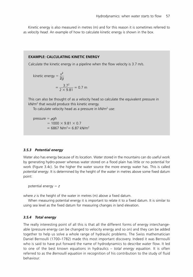
Kinetic energy is also measured in metres (m) and for this reason it is sometimes referred toas velocity head. An example of how to calculate kinetic energy is shown in the box.
Hydrodynamics: when water starts to flow 57
EXAMPLE: CALCULATING KINETIC ENERGY
Calculate the kinetic energy in a pipeline when the flow velocity is 3.7 m/s.
kinetic energy �
� � 0.7 m
This can also be thought of as a velocity head so calculate the equivalent pressure inkN/m2 that would produce this kinetic energy.
To calculate velocity head as a pressure in kN/m2 use:
pressure �
� 1000 � 9.81 � 0.7� 6867 N/m2� 6.87 kN/m2
�gh
3.72
2 � 9.81
v2
2g
3.5.3 Potential energy
Water also has energy because of its location. Water stored in the mountains can do useful workby generating hydro-power whereas water stored on a flood plain has little or no potential forwork (Figure 3.4c). So the higher the water source the more energy water has. This is calledpotential energy. It is determined by the height of the water in metres above some fixed datumpoint:
potential energy � z
where z is the height of the water in metres (m) above a fixed datum.When measuring potential energy it is important to relate it to a fixed datum. It is similar to
using sea level as the fixed datum for measuring changes in land elevation.
3.5.4 Total energy
The really interesting point of all this is that all the different forms of energy interchange-able (pressure energy can be changed to velocity energy and so on) and they can be addedtogether to help us solve a whole range of hydraulic problems. The Swiss mathematicianDaniel Bernoulli (1700–1782) made this most important discovery. Indeed it was Bernoulliwho is said to have put forward the name of hydrodynamics to describe water flow. It ledto one of the best known equations in hydraulics – total energy equation. It is oftenreferred to as the Bernoulli equation in recognition of his contribution to the study of fluidbehaviour.
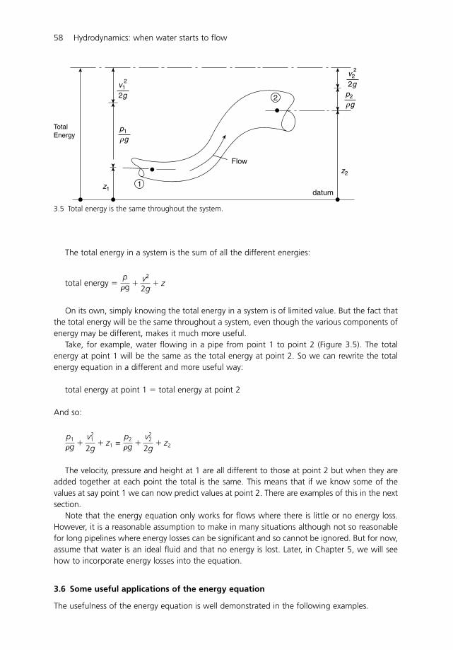
The total energy in a system is the sum of all the different energies:
total energy �
On its own, simply knowing the total energy in a system is of limited value. But the fact thatthe total energy will be the same throughout a system, even though the various components ofenergy may be different, makes it much more useful.
Take, for example, water flowing in a pipe from point 1 to point 2 (Figure 3.5). The totalenergy at point 1 will be the same as the total energy at point 2. So we can rewrite the totalenergy equation in a different and more useful way:
total energy at point 1 � total energy at point 2
And so:
=
The velocity, pressure and height at 1 are all different to those at point 2 but when they areadded together at each point the total is the same. This means that if we know some of thevalues at say point 1 we can now predict values at point 2. There are examples of this in the nextsection.
Note that the energy equation only works for flows where there is little or no energy loss.However, it is a reasonable assumption to make in many situations although not so reasonablefor long pipelines where energy losses can be significant and so cannot be ignored. But for now,assume that water is an ideal fluid and that no energy is lost. Later, in Chapter 5, we will seehow to incorporate energy losses into the equation.
3.6 Some useful applications of the energy equation
The usefulness of the energy equation is well demonstrated in the following examples.
p2
�g �
v22
2g � z2
p1
�g �
v21
2g � z1
p�g �
v2
2g � z
58 Hydrodynamics: when water starts to flow
3.5 Total energy is the same throughout the system.
TotalEnergy
1
2
datum
Flow
v12
2g
v22
2gp2
�g
p1
z1
z2
�g
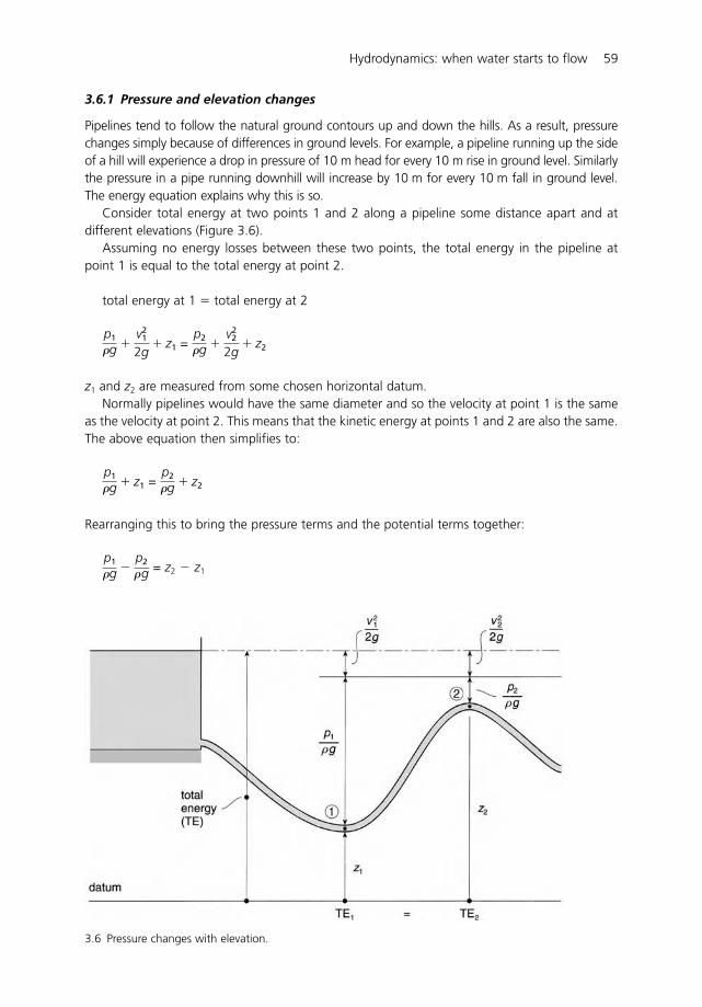
3.6.1 Pressure and elevation changes
Pipelines tend to follow the natural ground contours up and down the hills. As a result, pressurechanges simply because of differences in ground levels. For example, a pipeline running up the sideof a hill will experience a drop in pressure of 10 m head for every 10 m rise in ground level. Similarlythe pressure in a pipe running downhill will increase by 10 m for every 10 m fall in ground level.The energy equation explains why this is so.
Consider total energy at two points 1 and 2 along a pipeline some distance apart and atdifferent elevations (Figure 3.6).
Assuming no energy losses between these two points, the total energy in the pipeline atpoint 1 is equal to the total energy at point 2.
total energy at 1 � total energy at 2
=
z1 and z2 are measured from some chosen horizontal datum.Normally pipelines would have the same diameter and so the velocity at point 1 is the same
as the velocity at point 2. This means that the kinetic energy at points 1 and 2 are also the same.The above equation then simplifies to:
=
Rearranging this to bring the pressure terms and the potential terms together:
= z2 � z1p1
�g �
p2
�g
p2
�g � z2p1
�g � z1
p2
�g �
v22
2g � z2
p1
�g �
v21
2g � z1
Hydrodynamics: when water starts to flow 59
3.6 Pressure changes with elevation.
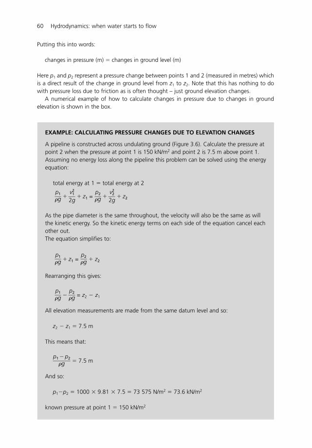
Putting this into words:
changes in pressure (m) � changes in ground level (m)
Here p1 and p2 represent a pressure change between points 1 and 2 (measured in metres) whichis a direct result of the change in ground level from z1 to z2. Note that this has nothing to dowith pressure loss due to friction as is often thought – just ground elevation changes.
A numerical example of how to calculate changes in pressure due to changes in groundelevation is shown in the box.
60 Hydrodynamics: when water starts to flow
EXAMPLE: CALCULATING PRESSURE CHANGES DUE TO ELEVATION CHANGES
A pipeline is constructed across undulating ground (Figure 3.6). Calculate the pressure atpoint 2 when the pressure at point 1 is 150 kN/m2 and point 2 is 7.5 m above point 1.Assuming no energy loss along the pipeline this problem can be solved using the energyequation:
total energy at 1 � total energy at 2
=
As the pipe diameter is the same throughout, the velocity will also be the same as willthe kinetic energy. So the kinetic energy terms on each side of the equation cancel eachother out.The equation simplifies to:
=
Rearranging this gives:
= z2 � z1
All elevation measurements are made from the same datum level and so:
z2 � z1 � 7.5 m
This means that:
� 7.5 m
And so:
p1�p2 � 1000 � 9.81 � 7.5 � 73 575 N/m2 � 73.6 kN/m2
known pressure at point 1 � 150 kN/m2
p1
�
p2
�g
p1
�g �
p2
�g
p2
�g � z2p1
�g � z1
p2
�g �
v22
2g � z2
p1
�g �
v21
2g � z1
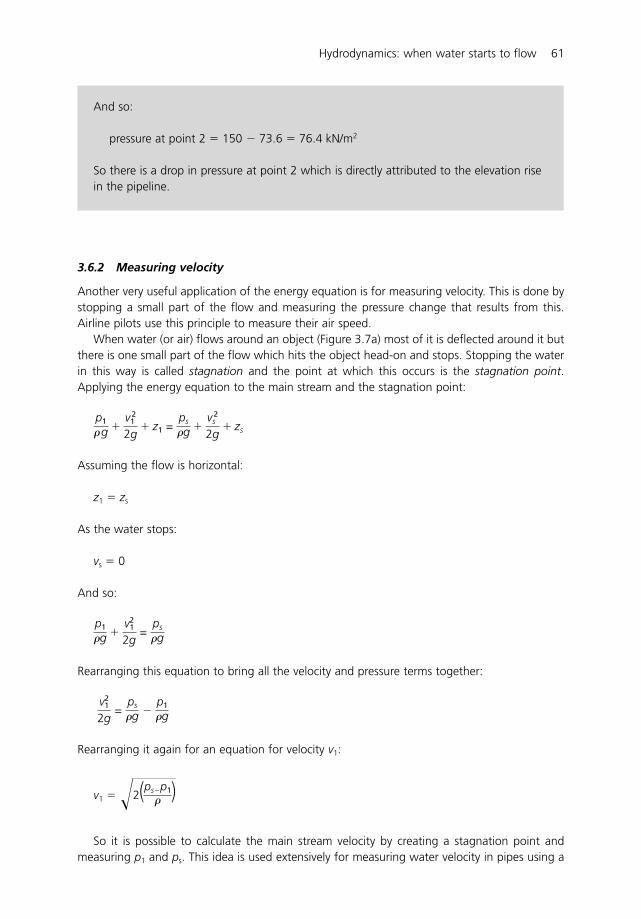
3.6.2 Measuring velocity
Another very useful application of the energy equation is for measuring velocity. This is done bystopping a small part of the flow and measuring the pressure change that results from this.Airline pilots use this principle to measure their air speed.
When water (or air) flows around an object (Figure 3.7a) most of it is deflected around it butthere is one small part of the flow which hits the object head-on and stops. Stopping the waterin this way is called stagnation and the point at which this occurs is the stagnation point.Applying the energy equation to the main stream and the stagnation point:
=
Assuming the flow is horizontal:
z1 � zs
As the water stops:
vs � 0
And so:
=
Rearranging this equation to bring all the velocity and pressure terms together:
=
Rearranging it again for an equation for velocity v1:
v1 �
So it is possible to calculate the main stream velocity by creating a stagnation point andmeasuring p1 and ps. This idea is used extensively for measuring water velocity in pipes using a
�2(ps�p1� )
ps
�g � p1
�gv2
1
2g
ps
�gp1
�g �
v21
2g
ps
�g �
v 2s
2g � zs
p1
�g �
v 21
2g � z1
Hydrodynamics: when water starts to flow 61
And so:
pressure at point 2 � 150 � 73.6 � 76.4 kN/m2
So there is a drop in pressure at point 2 which is directly attributed to the elevation risein the pipeline.
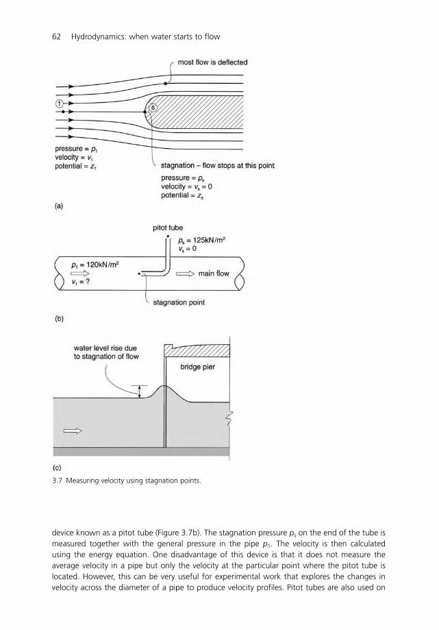
62 Hydrodynamics: when water starts to flow
3.7 Measuring velocity using stagnation points.
device known as a pitot tube (Figure 3.7b). The stagnation pressure ps on the end of the tube ismeasured together with the general pressure in the pipe p1. The velocity is then calculatedusing the energy equation. One disadvantage of this device is that it does not measure theaverage velocity in a pipe but only the velocity at the particular point where the pitot tube islocated. However, this can be very useful for experimental work that explores the changes invelocity across the diameter of a pipe to produce velocity profiles. Pitot tubes are also used on
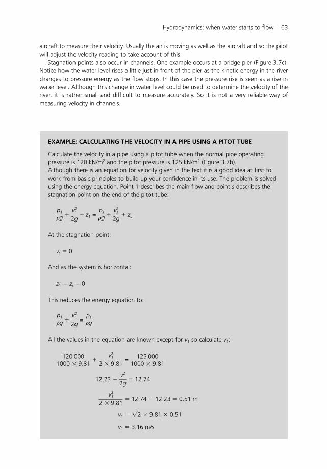
aircraft to measure their velocity. Usually the air is moving as well as the aircraft and so the pilotwill adjust the velocity reading to take account of this.
Stagnation points also occur in channels. One example occurs at a bridge pier (Figure 3.7c).Notice how the water level rises a little just in front of the pier as the kinetic energy in the riverchanges to pressure energy as the flow stops. In this case the pressure rise is seen as a rise inwater level. Although this change in water level could be used to determine the velocity of theriver, it is rather small and difficult to measure accurately. So it is not a very reliable way ofmeasuring velocity in channels.
Hydrodynamics: when water starts to flow 63
EXAMPLE: CALCULATING THE VELOCITY IN A PIPE USING A PITOT TUBE
Calculate the velocity in a pipe using a pitot tube when the normal pipe operatingpressure is 120 kN/m2 and the pitot pressure is 125 kN/m2 (Figure 3.7b).Although there is an equation for velocity given in the text it is a good idea at first towork from basic principles to build up your confidence in its use. The problem is solvedusing the energy equation. Point 1 describes the main flow and point s describes thestagnation point on the end of the pitot tube:
=
At the stagnation point:
vs � 0
And as the system is horizontal:
z1 � zs � 0
This reduces the energy equation to:
=
All the values in the equation are known except for v1 so calculate v1:
=
� 12.74
� 12.74 � 12.23 � 0.51 m
v1 �
v1 � 3.16 m/s
�2 � 9.81 � 0.51
v21
2 � 9.81
12.23 � v2
1
2g
125 0001000 � 9.81
120 0001000 � 9.81
� v2
1
2 � 9.81
ps
�gp1
�g �
v21
2g
ps
�g �
v2s
2g � zs
p1
�g �
v21
2g � z1

3.6.3 Orifices
Orifices are usually gated openings at the bottom of tanks and reservoirs used to control the releaseof water flow into a channel or some other collecting basin (Figure 3.8a). They are mostly rectan-gular or circular openings. The energy equation makes it possible to calculate the discharge releasedthrough an orifice by first calculating the flow velocity from the orifice and then multiplying it bythe area of the opening. One important proviso at this stage is that the orifice must discharge freelyand unhindered into the atmosphere, otherwise this approach will not work. Some orifices do oper-ate in submerged conditions and this does affect the flow. But this is described later in Section 7.2.
The energy equation for a tank with an orifice (Figure 3.8a) is written as:
=
Note the careful choice of the points for writing the energy terms. Point 1 is chosen at thewater surface in the tank and point 0 is at the centre of the orifice.
p0
�g �
v20
2g � z0
p1
�g �
v21
2g � z1
64 Hydrodynamics: when water starts to flow
3.8 Flow through orifices.
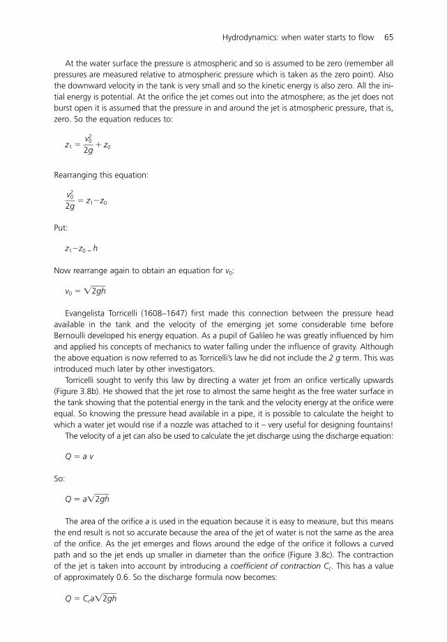
At the water surface the pressure is atmospheric and so is assumed to be zero (remember allpressures are measured relative to atmospheric pressure which is taken as the zero point). Alsothe downward velocity in the tank is very small and so the kinetic energy is also zero. All the ini-tial energy is potential. At the orifice the jet comes out into the atmosphere; as the jet does notburst open it is assumed that the pressure in and around the jet is atmospheric pressure, that is,zero. So the equation reduces to:
z1 �
Rearranging this equation:
� z1�z0
Put:
z1�z0 � h
Now rearrange again to obtain an equation for v0:
v0 �
Evangelista Torricelli (1608–1647) first made this connection between the pressure headavailable in the tank and the velocity of the emerging jet some considerable time beforeBernoulli developed his energy equation. As a pupil of Galileo he was greatly influenced by himand applied his concepts of mechanics to water falling under the influence of gravity. Althoughthe above equation is now referred to as Torricelli’s law he did not include the 2 g term. This wasintroduced much later by other investigators.
Torricelli sought to verify this law by directing a water jet from an orifice vertically upwards(Figure 3.8b). He showed that the jet rose to almost the same height as the free water surface inthe tank showing that the potential energy in the tank and the velocity energy at the orifice wereequal. So knowing the pressure head available in a pipe, it is possible to calculate the height towhich a water jet would rise if a nozzle was attached to it – very useful for designing fountains!
The velocity of a jet can also be used to calculate the jet discharge using the discharge equation:
Q � a v
So:
Q �
The area of the orifice a is used in the equation because it is easy to measure, but this meansthe end result is not so accurate because the area of the jet of water is not the same as the areaof the orifice. As the jet emerges and flows around the edge of the orifice it follows a curvedpath and so the jet ends up smaller in diameter than the orifice (Figure 3.8c). The contractionof the jet is taken into account by introducing a coefficient of contraction Cc. This has a valueof approximately 0.6. So the discharge formula now becomes:
Q � Cca�2gh
a�2gh
�2gh
v20
2g
v20
2g � z0
Hydrodynamics: when water starts to flow 65
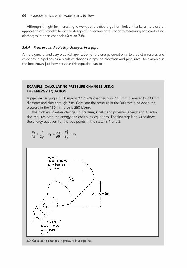
Although it might be interesting to work out the discharge from holes in tanks, a more usefulapplication of Torricelli’s law is the design of underflow gates for both measuring and controllingdischarges in open channels (Section 7.8).
3.6.4 Pressure and velocity changes in a pipe
A more general and very practical application of the energy equation is to predict pressures andvelocities in pipelines as a result of changes in ground elevation and pipe sizes. An example inthe box shows just how versatile this equation can be.
66 Hydrodynamics: when water starts to flow
EXAMPLE: CALCULATING PRESSURE CHANGES USING THE ENERGY EQUATION
A pipeline carrying a discharge of 0.12 m3/s changes from 150 mm diameter to 300 mmdiameter and rises through 7 m. Calculate the pressure in the 300 mm pipe when thepressure in the 150 mm pipe is 350 kN/m2.
This problem involves changes in pressure, kinetic and potential energy and its solu-tion requires both the energy and continuity equations. The first step is to write downthe energy equation for the two points in the systems 1 and 2:
=p2
�g �
v22
2g � z2
p1
�g �
v21
2g � z1
3.9 Calculating changes in pressure in a pipeline.
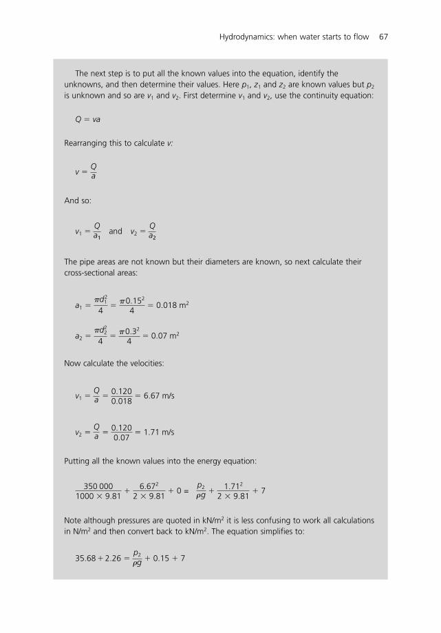
Hydrodynamics: when water starts to flow 67
The next step is to put all the known values into the equation, identify theunknowns, and then determine their values. Here p1, z1 and z2 are known values but p2
is unknown and so are v1 and v2. First determine v1 and v2, use the continuity equation:
Q � va
Rearranging this to calculate v:
v �
And so:
v1 � and v2 �
The pipe areas are not known but their diameters are known, so next calculate theircross-sectional areas:
a1 � � � 0.018 m2
a2 � � � 0.07 m2
Now calculate the velocities:
v1 � � 6.67 m/s
v2 � � � 1.71 m/s
Putting all the known values into the energy equation:
=
Note although pressures are quoted in kN/m2 it is less confusing to work all calculationsin N/m2 and then convert back to kN/m2. The equation simplifies to:
35.68 � 2.26 �p2
�g � 0.15 � 7
p2
�g � 1.712
2 � 9.81 � 7350 000
1000 � 9.81 � 6.672
2 � 9.81 � 0
0.1200.07
Qa
Qa � 0.120
0.018
�0.32
4�d2
2
4
�0.152
4�d1
2
4
Qa2
Qa1
Qa
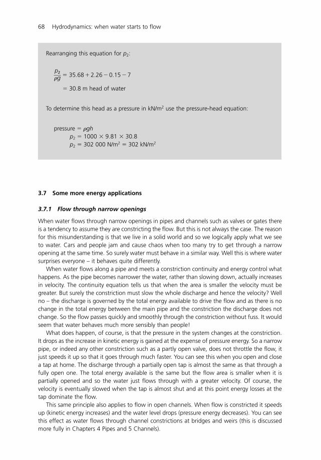
3.7 Some more energy applications
3.7.1 Flow through narrow openings
When water flows through narrow openings in pipes and channels such as valves or gates thereis a tendency to assume they are constricting the flow. But this is not always the case. The reasonfor this misunderstanding is that we live in a solid world and so we logically apply what we seeto water. Cars and people jam and cause chaos when too many try to get through a narrowopening at the same time. So surely water must behave in a similar way. Well this is where watersurprises everyone – it behaves quite differently.
When water flows along a pipe and meets a constriction continuity and energy control whathappens. As the pipe becomes narrower the water, rather than slowing down, actually increasesin velocity. The continuity equation tells us that when the area is smaller the velocity must begreater. But surely the constriction must slow the whole discharge and hence the velocity? Wellno – the discharge is governed by the total energy available to drive the flow and as there is nochange in the total energy between the main pipe and the constriction the discharge does notchange. So the flow passes quickly and smoothly through the constriction without fuss. It wouldseem that water behaves much more sensibly than people!
What does happen, of course, is that the pressure in the system changes at the constriction.It drops as the increase in kinetic energy is gained at the expense of pressure energy. So a narrowpipe, or indeed any other constriction such as a partly open valve, does not throttle the flow, itjust speeds it up so that it goes through much faster. You can see this when you open and closea tap at home. The discharge through a partially open tap is almost the same as that through afully open one. The total energy available is the same but the flow area is smaller when it ispartially opened and so the water just flows through with a greater velocity. Of course, thevelocity is eventually slowed when the tap is almost shut and at this point energy losses at thetap dominate the flow.
This same principle also applies to flow in open channels. When flow is constricted it speedsup (kinetic energy increases) and the water level drops (pressure energy decreases). You can seethis effect as water flows through channel constrictions at bridges and weirs (this is discussedmore fully in Chapters 4 Pipes and 5 Channels).
68 Hydrodynamics: when water starts to flow
Rearranging this equation for p2:
� 35.68 � 2.26 � 0.15 � 7
� 30.8 m head of water
To determine this head as a pressure in kN/m2 use the pressure-head equation:
pressure �
p2 � 1000 � 9.81 � 30.8p2 � 302 000 N/m2 � 302 kN/m2
�gh
p2
�g
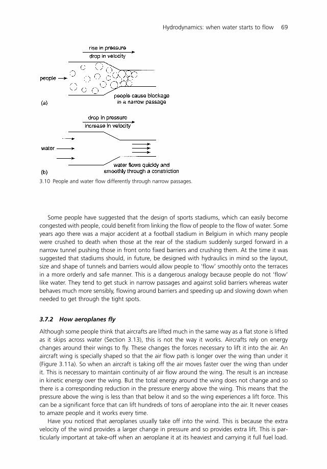
Some people have suggested that the design of sports stadiums, which can easily becomecongested with people, could benefit from linking the flow of people to the flow of water. Someyears ago there was a major accident at a football stadium in Belgium in which many peoplewere crushed to death when those at the rear of the stadium suddenly surged forward in anarrow tunnel pushing those in front onto fixed barriers and crushing them. At the time it wassuggested that stadiums should, in future, be designed with hydraulics in mind so the layout,size and shape of tunnels and barriers would allow people to ‘flow’ smoothly onto the terracesin a more orderly and safe manner. This is a dangerous analogy because people do not ‘flow’like water. They tend to get stuck in narrow passages and against solid barriers whereas waterbehaves much more sensibly, flowing around barriers and speeding up and slowing down whenneeded to get through the tight spots.
3.7.2 How aeroplanes fly
Although some people think that aircrafts are lifted much in the same way as a flat stone is liftedas it skips across water (Section 3.13), this is not the way it works. Aircrafts rely on energychanges around their wings to fly. These changes the forces necessary to lift it into the air. Anaircraft wing is specially shaped so that the air flow path is longer over the wing than under it(Figure 3.11a). So when an aircraft is taking off the air moves faster over the wing than underit. This is necessary to maintain continuity of air flow around the wing. The result is an increasein kinetic energy over the wing. But the total energy around the wing does not change and sothere is a corresponding reduction in the pressure energy above the wing. This means that thepressure above the wing is less than that below it and so the wing experiences a lift force. Thiscan be a significant force that can lift hundreds of tons of aeroplane into the air. It never ceasesto amaze people and it works every time.
Have you noticed that aeroplanes usually take off into the wind. This is because the extravelocity of the wind provides a larger change in pressure and so provides extra lift. This is par-ticularly important at take-off when an aeroplane it at its heaviest and carrying it full fuel load.
Hydrodynamics: when water starts to flow 69
3.10 People and water flow differently through narrow passages.
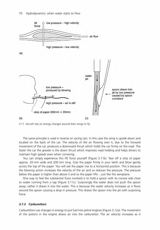
The same principle is used in reverse on racing cars. In this case the wing is upside down andlocated on the back of the car. The velocity of the air flowing over it, due to the forwardmovement of the car, produces a downward thrust which holds the car firmly on the road. Thefaster the car the greater is the down thrust which improves road holding and helps drivers tomaintain high speeds even when cornering.
You can simply experience this lift force yourself (Figure 3.11b). Tear off a strip of paperapprox. 20 mm wide and 200 mm long. Grip the paper firmly in your teeth and blow gentlyacross the top of the paper. You will see the paper rise to a horizontal position. This is becausethe blowing action increases the velocity of the air and so reduces the pressure. The pressurebelow the paper is higher than above it and so the paper lifts – just like the aeroplane.
One way to feel the substantial force involved is to hold a spoon with its convex side closeto water running from a tap (Figure 3.11c). Surprisingly the water does not push the spoonaway; rather it draws it into the water. This is because the water velocity increases as it flowsaround the spoon causing a drop in pressure. This draws the spoon into the jet with surprisingforce.
3.7.3 Carburettors
Carburettors use changes in energy to put fuel into petrol engines (Figure 3.12a). The movementof the pistons in the engine draws air into the carburettor. The air velocity increases as it
70 Hydrodynamics: when water starts to flow
3.11 Aircraft rely on energy changes around their wings to fly.
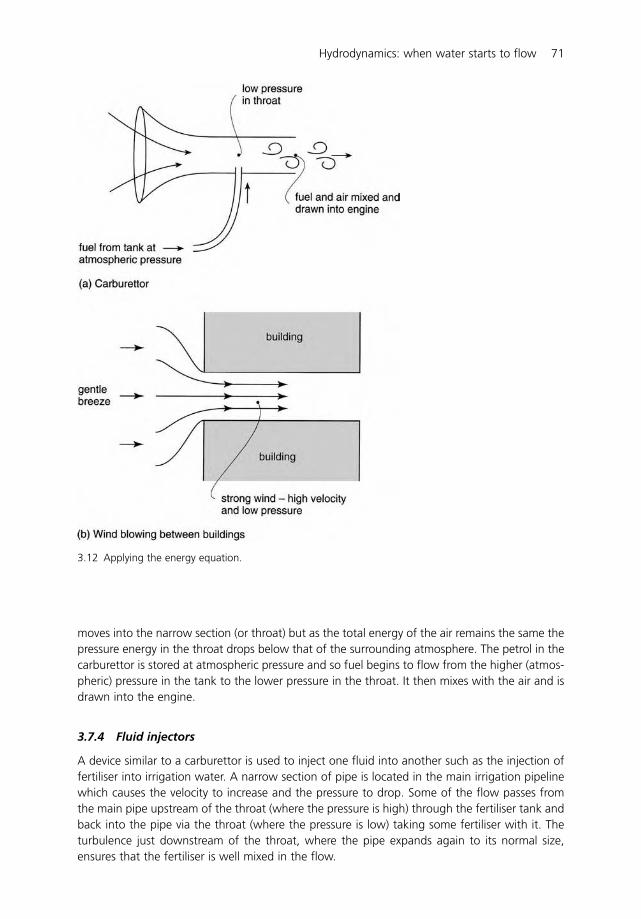
moves into the narrow section (or throat) but as the total energy of the air remains the same thepressure energy in the throat drops below that of the surrounding atmosphere. The petrol in thecarburettor is stored at atmospheric pressure and so fuel begins to flow from the higher (atmos-pheric) pressure in the tank to the lower pressure in the throat. It then mixes with the air and isdrawn into the engine.
3.7.4 Fluid injectors
A device similar to a carburettor is used to inject one fluid into another such as the injection offertiliser into irrigation water. A narrow section of pipe is located in the main irrigation pipelinewhich causes the velocity to increase and the pressure to drop. Some of the flow passes fromthe main pipe upstream of the throat (where the pressure is high) through the fertiliser tank andback into the pipe via the throat (where the pressure is low) taking some fertiliser with it. Theturbulence just downstream of the throat, where the pipe expands again to its normal size,ensures that the fertiliser is well mixed in the flow.
Hydrodynamics: when water starts to flow 71
3.12 Applying the energy equation.
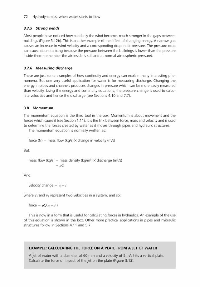
3.7.5 Strong winds
Most people have noticed how suddenly the wind becomes much stronger in the gaps betweenbuildings (Figure 3.12b). This is another example of the effect of changing energy. A narrow gapcauses an increase in wind velocity and a corresponding drop in air pressure. The pressure dropcan cause doors to bang because the pressure between the buildings is lower than the pressureinside them (remember the air inside is still and at normal atmospheric pressure).
3.7.6 Measuring discharge
These are just some examples of how continuity and energy can explain many interesting phe-nomena. But one very useful application for water is for measuring discharge. Changing theenergy in pipes and channels produces changes in pressure which can be more easily measuredthan velocity. Using the energy and continuity equations, the pressure change is used to calcu-late velocities and hence the discharge (see Sections 4.10 and 7.7).
3.8 Momentum
The momentum equation is the third tool in the box. Momentum is about movement and theforces which cause it (see Section 1.11). It is the link between force, mass and velocity and is usedto determine the forces created by water as it moves through pipes and hydraulic structures.
The momentum equation is normally written as:
force (N) � mass flow (kg/s) � change in velocity (m/s)
But:
mass flow (kg/s) � mass density (kg/m3) � discharge (m3/s)� �Q
And:
velocity change � v2�v1
where v1 and v2 represent two velocities in a system, and so:
force � �Q(v2�v1)
This is now in a form that is useful for calculating forces in hydraulics. An example of the useof this equation is shown in the box. Other more practical applications in pipes and hydraulicstructures follow in Sections 4.11 and 5.7.
72 Hydrodynamics: when water starts to flow
EXAMPLE: CALCULATING THE FORCE ON A PLATE FROM A JET OF WATER
A jet of water with a diameter of 60 mm and a velocity of 5 m/s hits a vertical plate.Calculate the force of impact of the jet on the plate (Figure 3.13).
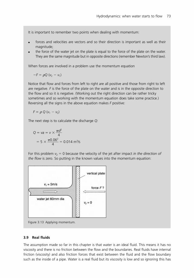
Hydrodynamics: when water starts to flow 73
It is important to remember two points when dealing with momentum:
� forces and velocities are vectors and so their direction is important as well as theirmagnitude;
� the force of the water jet on the plate is equal to the force of the plate on the water.They are the same magnitude but in opposite directions (remember Newton’s third law).
When forces are involved in a problem use the momentum equation
�F � ρQ (v2 � v1)
Notice that flow and forces from left to right are all positive and those from right to leftare negative. F is the force of the plate on the water and is in the opposite direction tothe flow and so it is negative. (Working out the right direction can be rather trickysometimes and so working with the momentum equation does take some practice.)Reversing all the signs in the above equation makes F positive:
F � ρ Q (v1 � v2)
The next step is to calculate the discharge Q:
Q � va � v �
� 5 � � 0.014 m3/s
For this problem v2 � 0 because the velocity of the jet after impact in the direction ofthe flow is zero. So putting in the known values into the momentum equation:
F � 1000 � 0.014 � 5F � 70 N
�0.062
4
�d2
4
3.9 Real fluids
The assumption made so far in this chapter is that water is an ideal fluid. This means it has noviscosity and there is no friction between the flow and the boundaries. Real fluids have internalfriction (viscosity) and also friction forces that exist between the fluid and the flow boundarysuch as the inside of a pipe. Water is a real fluid but its viscosity is low and so ignoring this has
Figure 3.13 Applying momentum.

little or no effect on the design of pipes and channels. However the friction between the flowand the boundary is important and cannot be ignored for design purposes. We use a modifiedversion of the energy equation to take account of this.
3.9.1 Taking account of energy losses
When water flows along pipes and channels energy is lost from friction between the water andits boundaries; we can account for this in the energy equation. Writing the energy equation forpoints 1 and 2 along a pipeline carrying a real fluid needs an additional term hf to describe theenergy loss between them:
� � hf
hf is the most important element in this equation for determining the size of pipe or channelneeded to carry a given flow. The question is how to measure or calculate it and what factorsinfluence its value. This was the challenge faced by 19th century scientists investigating fluidflow and the results of their work now form the basis of all pipe and channel design procedures.But more about this in Chapters 4 and 5.
3.9.2 Cavitation
Real fluids suffer from cavitation and it can cause lots of problems, particularly in pumps andcontrol valves. It occurs when a fluid is moving very fast; as a consequence, the pressure candrop to very low values approaching zero (vacuum pressure).
The control valve on a pipeline provides a good example (Figure 3.14a). When the valve isalmost closed the water velocity under the gate can be very high. This also means high kineticenergy and this is gained at the expense of the pressure energy. If the pressure drops below thevapour pressure of water (this is approximately 0.3 m absolute) bubbles, called cavities, start toform in the water. They are very small (less than 0.5 mm in diameter) but there are manythousands of them and give the water a milky appearance. The bubbles are filled with watervapour and the pressure inside them is very low. But as the bubbles move under the gate andinto the pipe downstream, the velocity slows, the pressure rises and the bubbles begin tocollapse. It is at this point that the danger arises. If the bubbles collapse in the main flow theydo no harm, but if they are close to the pipe wall they can do a great deal of damage. Noticethe way in which the bubbles collapse (Figure 3.14b). As the bubble becomes unstable a tinyneedle jet of water rushes across the cavity and it is this which can do great damage even tosteel and concrete because the pressure under the jet can be as high as 4000 bar! See Section 8.4.4for more details of cavitation in pumps.
Some people confuse cavitation with air entrainment, but it is a very different phenomenon.Air entrainment occurs when there is turbulence at hydraulic structures and air bubbles aredrawn into the flow. The milky appearance of the water is similar but the bubbles are air filledand will do no harm to pumps and valves.
3.9.3 Boundary layers
Friction between water flow and its boundaries and the internal friction (viscosity) within thewater gives rise to an effect known as the boundary layer. Water flowing in a pipe moves fasterin the middle of the pipe than near the pipe wall. This is because friction between the water and
p2
�g �
v22
2g � z2
p1
�g �
v21
2g � z1
74 Hydrodynamics: when water starts to flow
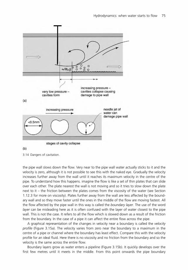
the pipe wall slows down the flow. Very near to the pipe wall water actually sticks to it and thevelocity is zero, although it is not possible to see this with the naked eye. Gradually the velocityincreases further away from the wall until it reaches its maximum velocity in the centre of thepipe. To understand how this happens. imagine the flow is like a set of thin plates that can slideover each other. The plate nearest the wall is not moving and so it tries to slow down the platenext to it – the friction between the plates comes from the viscosity of the water (see Section1.12.3 for more on viscosity). Plates further away from the wall are less affected by the bound-ary wall and so they move faster until the ones in the middle of the flow are moving fastest. Allthe flow affected by the pipe wall in this way is called the boundary layer. The use of the wordlayer can be misleading here as it is often confused with the layer of water closest to the pipewall. This is not the case. It refers to all the flow which is slowed down as a result of the frictionfrom the boundary. In the case of a pipe it can affect the entire flow across the pipe.
A graphical representation of the changes in velocity near a boundary is called the velocityprofile (Figure 3.15a). The velocity varies from zero near the boundary to a maximum in thecentre of a pipe or channel where the boundary has least effect. Compare this with the velocityprofile for an ideal fluid. Here there is no viscosity and no friction from the boundary and so thevelocity is the same across the entire flow.
Boundary layers grow as water enters a pipeline (Figure 3.15b). It quickly develops over thefirst few metres until it meets in the middle. From this point onwards the pipe boundary
Hydrodynamics: when water starts to flow 75
3.14 Dangers of cavitation.
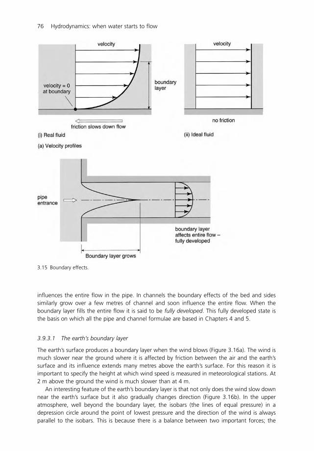
influences the entire flow in the pipe. In channels the boundary effects of the bed and sidessimilarly grow over a few metres of channel and soon influence the entire flow. When theboundary layer fills the entire flow it is said to be fully developed. This fully developed state isthe basis on which all the pipe and channel formulae are based in Chapters 4 and 5.
3.9.3.1 The earth’s boundary layer
The earth’s surface produces a boundary layer when the wind blows (Figure 3.16a). The wind ismuch slower near the ground where it is affected by friction between the air and the earth’ssurface and its influence extends many metres above the earth’s surface. For this reason it isimportant to specify the height at which wind speed is measured in meteorological stations. At2 m above the ground the wind is much slower than at 4 m.
An interesting feature of the earth’s boundary layer is that not only does the wind slow downnear the earth’s surface but it also gradually changes direction (Figure 3.16b). In the upperatmosphere, well beyond the boundary layer, the isobars (the lines of equal pressure) in adepression circle around the point of lowest pressure and the direction of the wind is alwaysparallel to the isobars. This is because there is a balance between two important forces; the
76 Hydrodynamics: when water starts to flow
3.15 Boundary effects.
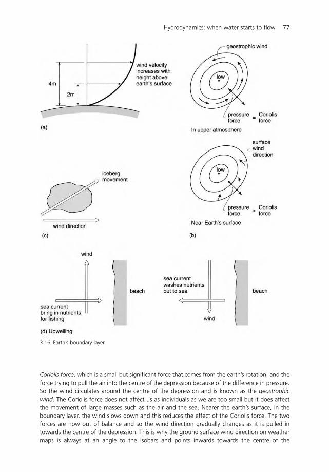
Coriolis force, which is a small but significant force that comes from the earth’s rotation, and theforce trying to pull the air into the centre of the depression because of the difference in pressure.So the wind circulates around the centre of the depression and is known as the geostrophicwind. The Coriolis force does not affect us as individuals as we are too small but it does affectthe movement of large masses such as the air and the sea. Nearer the earth’s surface, in theboundary layer, the wind slows down and this reduces the effect of the Coriolis force. The twoforces are now out of balance and so the wind direction gradually changes as it is pulled intowards the centre of the depression. This is why the ground surface wind direction on weathermaps is always at an angle to the isobars and points inwards towards the centre of the
Hydrodynamics: when water starts to flow 77
3.16 Earth’s boundary layer.
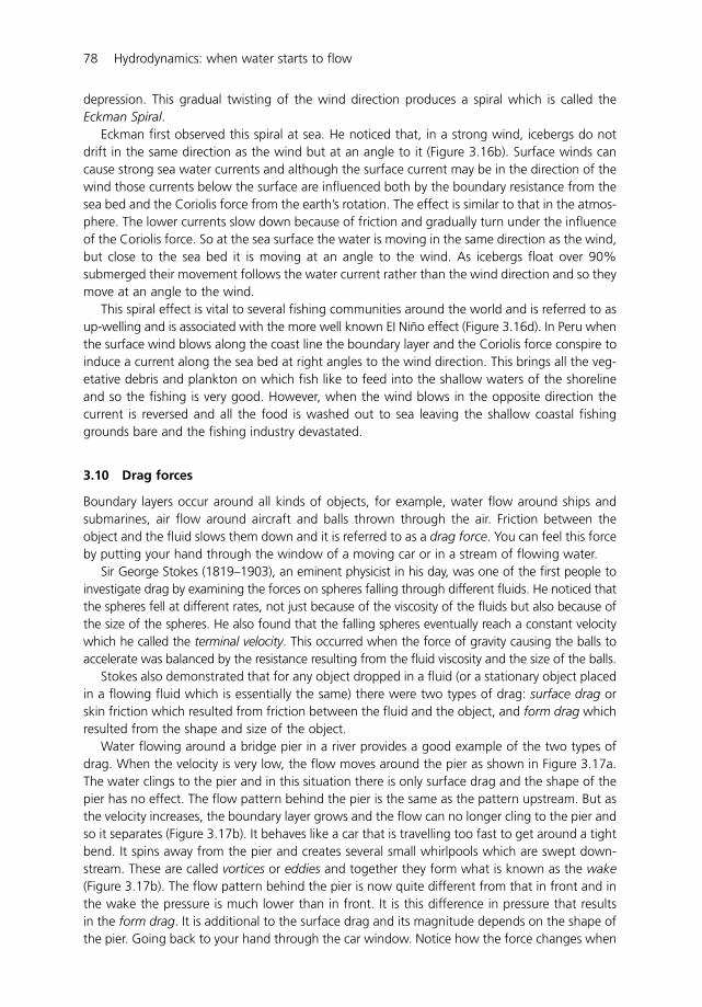
depression. This gradual twisting of the wind direction produces a spiral which is called theEckman Spiral.
Eckman first observed this spiral at sea. He noticed that, in a strong wind, icebergs do notdrift in the same direction as the wind but at an angle to it (Figure 3.16b). Surface winds cancause strong sea water currents and although the surface current may be in the direction of thewind those currents below the surface are influenced both by the boundary resistance from thesea bed and the Coriolis force from the earth’s rotation. The effect is similar to that in the atmos-phere. The lower currents slow down because of friction and gradually turn under the influenceof the Coriolis force. So at the sea surface the water is moving in the same direction as the wind,but close to the sea bed it is moving at an angle to the wind. As icebergs float over 90%submerged their movement follows the water current rather than the wind direction and so theymove at an angle to the wind.
This spiral effect is vital to several fishing communities around the world and is referred to asup-welling and is associated with the more well known EI Niño effect (Figure 3.16d). In Peru whenthe surface wind blows along the coast line the boundary layer and the Coriolis force conspire toinduce a current along the sea bed at right angles to the wind direction. This brings all the veg-etative debris and plankton on which fish like to feed into the shallow waters of the shorelineand so the fishing is very good. However, when the wind blows in the opposite direction thecurrent is reversed and all the food is washed out to sea leaving the shallow coastal fishinggrounds bare and the fishing industry devastated.
3.10 Drag forces
Boundary layers occur around all kinds of objects, for example, water flow around ships andsubmarines, air flow around aircraft and balls thrown through the air. Friction between theobject and the fluid slows them down and it is referred to as a drag force. You can feel this forceby putting your hand through the window of a moving car or in a stream of flowing water.
Sir George Stokes (1819–1903), an eminent physicist in his day, was one of the first people toinvestigate drag by examining the forces on spheres falling through different fluids. He noticed thatthe spheres fell at different rates, not just because of the viscosity of the fluids but also because ofthe size of the spheres. He also found that the falling spheres eventually reach a constant velocitywhich he called the terminal velocity. This occurred when the force of gravity causing the balls toaccelerate was balanced by the resistance resulting from the fluid viscosity and the size of the balls.
Stokes also demonstrated that for any object dropped in a fluid (or a stationary object placedin a flowing fluid which is essentially the same) there were two types of drag: surface drag orskin friction which resulted from friction between the fluid and the object, and form drag whichresulted from the shape and size of the object.
Water flowing around a bridge pier in a river provides a good example of the two types ofdrag. When the velocity is very low, the flow moves around the pier as shown in Figure 3.17a.The water clings to the pier and in this situation there is only surface drag and the shape of thepier has no effect. The flow pattern behind the pier is the same as the pattern upstream. But asthe velocity increases, the boundary layer grows and the flow can no longer cling to the pier andso it separates (Figure 3.17b). It behaves like a car that is travelling too fast to get around a tightbend. It spins away from the pier and creates several small whirlpools which are swept down-stream. These are called vortices or eddies and together they form what is known as the wake(Figure 3.17b). The flow pattern behind the pier is now quite different from that in front and inthe wake the pressure is much lower than in front. It is this difference in pressure that results in the form drag. It is additional to the surface drag and its magnitude depends on the shape ofthe pier. Going back to your hand through the car window. Notice how the force changes when
78 Hydrodynamics: when water starts to flow
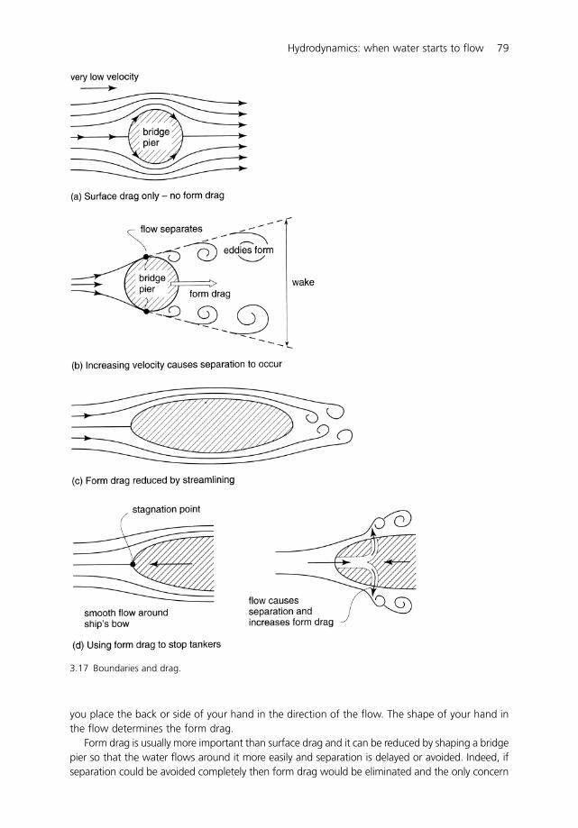
you place the back or side of your hand in the direction of the flow. The shape of your hand inthe flow determines the form drag.
Form drag is usually more important than surface drag and it can be reduced by shaping a bridgepier so that the water flows around it more easily and separation is delayed or avoided. Indeed, ifseparation could be avoided completely then form drag would be eliminated and the only concern
Hydrodynamics: when water starts to flow 79
3.17 Boundaries and drag.
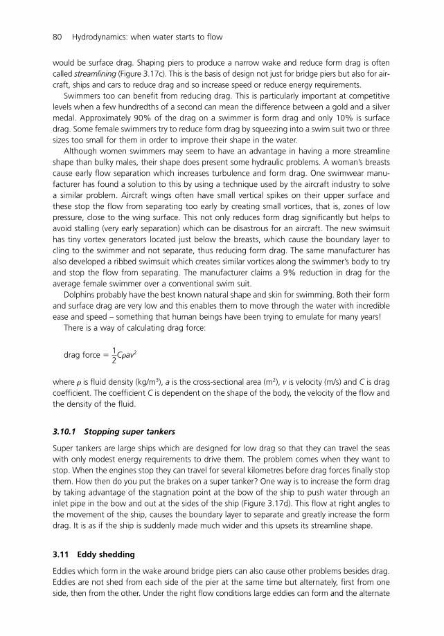
would be surface drag. Shaping piers to produce a narrow wake and reduce form drag is oftencalled streamlining (Figure 3.17c). This is the basis of design not just for bridge piers but also for air-craft, ships and cars to reduce drag and so increase speed or reduce energy requirements.
Swimmers too can benefit from reducing drag. This is particularly important at competitivelevels when a few hundredths of a second can mean the difference between a gold and a silvermedal. Approximately 90% of the drag on a swimmer is form drag and only 10% is surfacedrag. Some female swimmers try to reduce form drag by squeezing into a swim suit two or threesizes too small for them in order to improve their shape in the water.
Although women swimmers may seem to have an advantage in having a more streamlineshape than bulky males, their shape does present some hydraulic problems. A woman’s breastscause early flow separation which increases turbulence and form drag. One swimwear manu-facturer has found a solution to this by using a technique used by the aircraft industry to solvea similar problem. Aircraft wings often have small vertical spikes on their upper surface andthese stop the flow from separating too early by creating small vortices, that is, zones of lowpressure, close to the wing surface. This not only reduces form drag significantly but helps toavoid stalling (very early separation) which can be disastrous for an aircraft. The new swimsuithas tiny vortex generators located just below the breasts, which cause the boundary layer tocling to the swimmer and not separate, thus reducing form drag. The same manufacturer hasalso developed a ribbed swimsuit which creates similar vortices along the swimmer’s body to tryand stop the flow from separating. The manufacturer claims a 9% reduction in drag for theaverage female swimmer over a conventional swim suit.
Dolphins probably have the best known natural shape and skin for swimming. Both their formand surface drag are very low and this enables them to move through the water with incredibleease and speed – something that human beings have been trying to emulate for many years!
There is a way of calculating drag force:
drag force �
where � is fluid density (kg/m3), a is the cross-sectional area (m2), v is velocity (m/s) and C is dragcoefficient. The coefficient C is dependent on the shape of the body, the velocity of the flow andthe density of the fluid.
3.10.1 Stopping super tankers
Super tankers are large ships which are designed for low drag so that they can travel the seaswith only modest energy requirements to drive them. The problem comes when they want tostop. When the engines stop they can travel for several kilometres before drag forces finally stopthem. How then do you put the brakes on a super tanker? One way is to increase the form dragby taking advantage of the stagnation point at the bow of the ship to push water through aninlet pipe in the bow and out at the sides of the ship (Figure 3.17d). This flow at right angles tothe movement of the ship, causes the boundary layer to separate and greatly increase the formdrag. It is as if the ship is suddenly made much wider and this upsets its streamline shape.
3.11 Eddy shedding
Eddies which form in the wake around bridge piers can also cause other problems besides drag.Eddies are not shed from each side of the pier at the same time but alternately, first from oneside, then from the other. Under the right flow conditions large eddies can form and the alternate
12
C�av2
80 Hydrodynamics: when water starts to flow
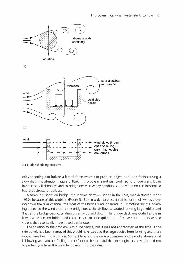
eddy-shedding can induce a lateral force which can push an object back and forth causing aslow rhythmic vibration (Figure 3.18a). This problem is not just confined to bridge piers. It canhappen to tall chimneys and to bridge decks in windy conditions. The vibration can become sobad that structures collapse.
A famous suspension bridge, the Tacoma Narrows Bridge in the USA, was destroyed in the1930s because of this problem (Figure 3.18b). In order to protect traffic from high winds blow-ing down the river channel, the sides of the bridge were boarded up. Unfortunately the board-ing deflected the wind around the bridge deck, the air flow separated forming large eddies andthis set the bridge deck oscillating violently up and down. The bridge deck was quite flexible asit was a suspension bridge and could in fact tolerate quite a lot of movement but this was soviolent that eventually it destroyed the bridge.
The solution to the problem was quite simple, but it was not appreciated at the time. If theside panels had been removed this would have stopped the large eddies from forming and therewould have been no vibration. So next time you are on a suspension bridge and a strong windis blowing and you are feeling uncomfortable be thankful that the engineers have decided notto protect you from the wind by boarding up the sides.
Hydrodynamics: when water starts to flow 81
3.18 Eddy shedding problems.
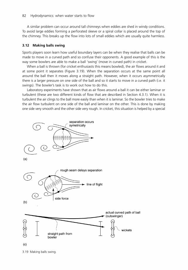
A similar problem can occur around tall chimneys when eddies are shed in windy conditions.To avoid large eddies forming a perforated sleeve or a spiral collar is placed around the top ofthe chimney. This breaks up the flow into lots of small eddies which are usually quite harmless.
3.12 Making balls swing
Sports players soon learn how useful boundary layers can be when they realise that balls can bemade to move in a curved path and so confuse their opponents. A good example of this is theway some bowlers are able to make a ball ‘swing’ (move in curved path) in cricket.
When a ball is thrown (for cricket enthusiasts this means bowled), the air flows around it andat some point it separates (Figure 3.19). When the separation occurs at the same point allaround the ball then it moves along a straight path. However, when it occurs asymmetricallythere is a larger pressure on one side of the ball and so it starts to move in a curved path (i.e. itswings). The bowler’s task is to work out how to do this.
Laboratory experiments have shown that as air flows around a ball it can be either laminar orturbulent (these are two different kinds of flow that are described in Section 4.3.1). When it isturbulent the air clings to the ball more easily than when it is laminar. So the bowler tries to makethe air flow turbulent on one side of the ball and laminar on the other. This is done by makingone side very smooth and the other side very rough. In cricket, this situation is helped by a special
82 Hydrodynamics: when water starts to flow
3.19 Making balls swing.
stitched seam around the middle of the ball which ensures that the ball is rough enough to createturbulent conditions. The ball is bowled so that the polished side of the ball is facing the bats-man and the seam is at an angle to the main direction of travel. The air flow on the smooth sideseparates earlier than on the rough side and so the ball swings towards the turbulent side. Thecross force can be up to 0.8 N depending on how fast the ball is travelling and may cause a swingof up to 0.6 m in 20 m – the length of a cricket pitch. This can be more than enough to seriouslyupset a batsman who may be expecting a straight ball. This is why bowlers seem to spend somuch of their time polishing the ball on their trousers prior to their run up in order to get it assmooth as possible to get the maximum swing. The swing may be in or out depending on howthe bowler holds the ball. However, not all the surprise is with the bowler. An observant batsmanmay know what is coming by looking to see how the bowler is holding the ball and so anticipatethe swing.
Sometimes strange things happen which even puzzle those who understand hydraulics. Justoccasionally bowlers have noticed that a ball that was meant to swing in towards the batsmanswings away from him instead – an outswinger. What happens is that when a ball is bowled fastenough the entire air flow around the ball turns turbulent and so the separation occurs muchearlier. The stitched seam around the ball now acts as a ramp causing the air to be pushed away,creating a side force in the opposite direction to what was expected. This causes great delight forthe bowler but it can give the batsman quite a fright. But most batsmen can relax as this specialswing only occurs when the ball reaches 130 to 150 km/h and only a few bowlers can actuallyreach this velocity. However, some unscrupulous bowlers have discovered a way of doing this atmuch lower velocities. By deliberately roughening the ball on one side (which is not allowed) andpolishing it on the other (which is allowed) they can bowl an outswinger at much lower velocities.This caused a major row in cricket in the early 1990s and again in 2006 when a Pakistani bowlerwas accused of deliberately roughening the ball. Imran Khan though was famous for his highspeed bowling and could produce outswingers without resorting to such tactics. It is of courseallowed for the ball to scuff or become rough naturally through play but this can take some time.
Causing a ball to spin at the same time as driving it forward can also add to the complexitiesof air flow and also to the excitement of ball sports. Some famous ball swings in recent yearsresulted in the goals scored by the Brazilian footballer, Roberto Carlos, in 1997 and by DavidBeckham in the 2006 World Cup games. In each case the goal area was completely blocked bythe opposing team players. As each player kicked the ball it seemed to be heading for the cornerflag but instead it followed a curved path around the defending players and into the goal. Theyachieved this amazing feat by striking the ball on its edge causing it to spin, which induced asideways force. This, together with the boundary layer effect and a great deal of skill (and a littleluck) produced some of the best goals ever scored.
3.13 Successful stone-skipping
Skipping stones across water has been a popular pastime for many thousands of years.Apparently the Greeks started it and according to the Guiness Book of Records the world recordis held by Kurt Steiner. It was set in 2003 at 40 rebounds.
Various parameters affect the number of skips such as the weight and shape of the stone,ideally this should be flat plate shape, and the velocity and spin. This was very much an art untilresearch undertaken at the Institutut de Researche sur les Phenomenones Hors Equilibre inMarseille and published in Nature in 2004 investigated the hydraulics of this past time. Amongthe many parameters investigated the most important one was the angle at which the stone hitsthe water. The ‘magic’ angle, as the researchers described it, was 20�and at this angle the energydissipated by the stone impact with the water is minimised. So at this angle you will achieve the
Hydrodynamics: when water starts to flow 83
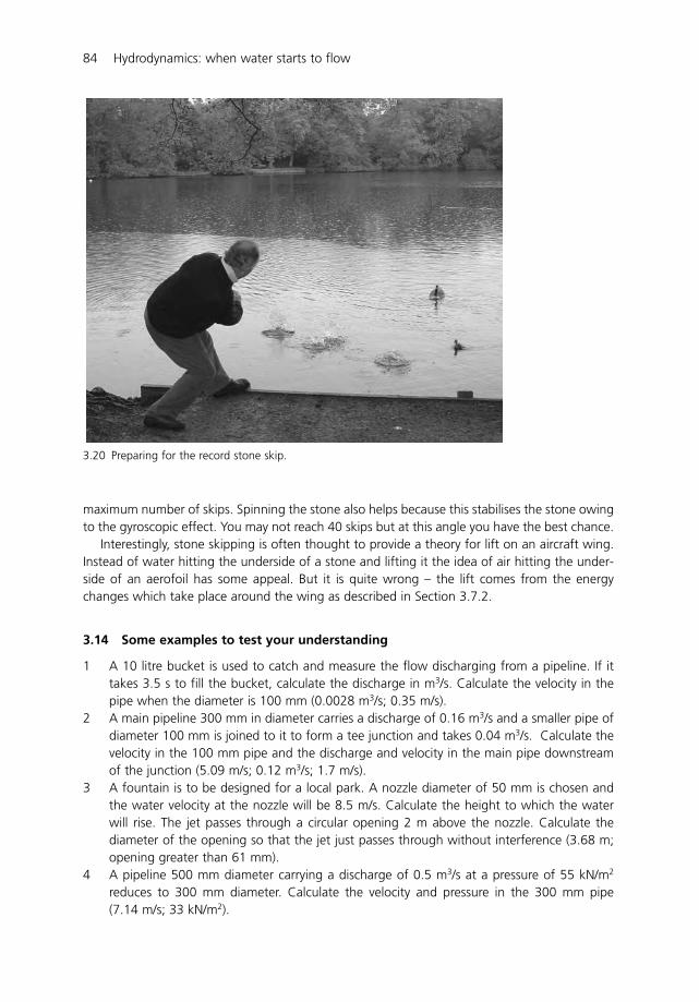
maximum number of skips. Spinning the stone also helps because this stabilises the stone owingto the gyroscopic effect. You may not reach 40 skips but at this angle you have the best chance.
Interestingly, stone skipping is often thought to provide a theory for lift on an aircraft wing.Instead of water hitting the underside of a stone and lifting it the idea of air hitting the under-side of an aerofoil has some appeal. But it is quite wrong – the lift comes from the energychanges which take place around the wing as described in Section 3.7.2.
3.14 Some examples to test your understanding
1 A 10 litre bucket is used to catch and measure the flow discharging from a pipeline. If ittakes 3.5 s to fill the bucket, calculate the discharge in m3/s. Calculate the velocity in thepipe when the diameter is 100 mm (0.0028 m3/s; 0.35 m/s).
2 A main pipeline 300 mm in diameter carries a discharge of 0.16 m3/s and a smaller pipe ofdiameter 100 mm is joined to it to form a tee junction and takes 0.04 m3/s. Calculate thevelocity in the 100 mm pipe and the discharge and velocity in the main pipe downstreamof the junction (5.09 m/s; 0.12 m3/s; 1.7 m/s).
3 A fountain is to be designed for a local park. A nozzle diameter of 50 mm is chosen andthe water velocity at the nozzle will be 8.5 m/s. Calculate the height to which the waterwill rise. The jet passes through a circular opening 2 m above the nozzle. Calculate thediameter of the opening so that the jet just passes through without interference (3.68 m;opening greater than 61 mm).
4 A pipeline 500 mm diameter carrying a discharge of 0.5 m3/s at a pressure of 55 kN/m2
reduces to 300 mm diameter. Calculate the velocity and pressure in the 300 mm pipe(7.14 m/s; 33 kN/m2).
84 Hydrodynamics: when water starts to flow
3.20 Preparing for the record stone skip.
4 Pipes
4.1 Introduction
Pipes are a common feature of water supply systems and have many advantages over openchannels. They are completely enclosed, usually circular in section and always flow full of water.This is in contrast to channels which are open to the atmosphere and can have many differentshapes and sizes – but more about channels in Chapter 5. One big advantage of pipes is thatwater can flow uphill as well as downhill so land topography is not such a constraint whentaking water from one location to another.
There are occasions when pipes do not flow full – one example is gravity flow sewers. Theytake sewage away from homes and factories and often only flow partially full under the forceof gravity in order to avoid pumping. They look like pipes and are indeed pipes but hydraulicallythey behave like open channels. The reason pipes are used for this purpose is that sewers areusually buried below ground to avoid public health problems and it would be difficult to buryan open channel!
4.2 A typical pipe flow problem
Pipe flow problems usually involve calculating the right size of pipe to use for a given discharge.A typical example is a water supply to a village (Figure 4.1). A pipeline connects a main storagereservoir to a small service (storage) tank just outside the village which then supplies water toindividual houses. The required discharge (Q m3/s) for the village is determined by the waterdemand of each user and the number of users being supplied. We now need to determine theright size of pipe to use to ensure that this discharge is supplied from the main storage reservoirto the service tank.
A formula to calculate pipe size would be ideal. However, to get there we first need to look atthe energy available to ‘push’ water through the system, so the place to start is the energy equa-tion. But this is a real fluid problem and so energy losses due to friction must be taken into account.So writing the energy equation for two points in this system – point 1 is at the main reservoir andpoint 2 at the service tank – and allowing for the energy loss as water flows between the two:
Points 1 and 2 are carefully chosen in order to simplify the equation and also the solution.Point 1 is at the surface of the main reservoir where the pressure p1 is atmospheric pressure and
p1
�g �
v21
2g � z1
�
p2
�g �
v22
2g � z2
� hf
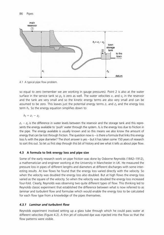
so equal to zero (remember we are working in gauge pressures). Point 2 is also at the watersurface in the service tank so p2 is zero as well. The water velocities v1 and v2 in the reservoirand the tank are very small and so the kinetic energy terms are also very small and can beassumed to be zero. This leaves just the potential energy terms z1 and z2 and the energy lossterm hf. So the energy equation simplifies down to:
hf � z1 � z2
z1 � z2 is the difference in water levels between the reservoir and the storage tank and this repre-sents the energy available to ‘push’ water through the system. hf is the energy loss due to friction inthe pipe. The energy available is usually known and so this means we also know the amount ofenergy that can be lost through friction. The question now is – is there a formula that links this energyloss hf with the pipe diameter? The short answer is yes – but it has taken some 150 years of researchto sort this out. So let us first step through this bit of history and see what it tells us about pipe flow.
4.3 A formula to link energy loss and pipe size
Some of the early research work on pipe friction was done by Osborne Reynolds (1842–1912),a mathematician and engineer working at the University in Manchester in UK. He measured thepressure loss in pipes of different lengths and diameters at different discharges with some inter-esting results. At low flows he found that the energy loss varied directly with the velocity. Sowhen the velocity was doubled the energy loss also doubled. But at high flows the energy lossvaried as the square of the velocity. So when the velocity was doubled the energy loss increasedfour-fold. Clearly, Reynolds was observing two quite different types of flow. This thinking led toReynolds classic experiment that established the difference between what is now referred to aslaminar and turbulent flow and formulae which would enable the energy loss to be calculatedfor each flow type from a knowledge of the pipes themselves.
4.3.1 Laminar and turbulent flow
Reynolds experiment involved setting up a glass tube through which he could pass water atdifferent velocities (Figure 4.2). A thin jet of coloured dye was injected into the flow so that theflow patterns were visible.
86 Pipes
4.1 A typical pipe flow problem.
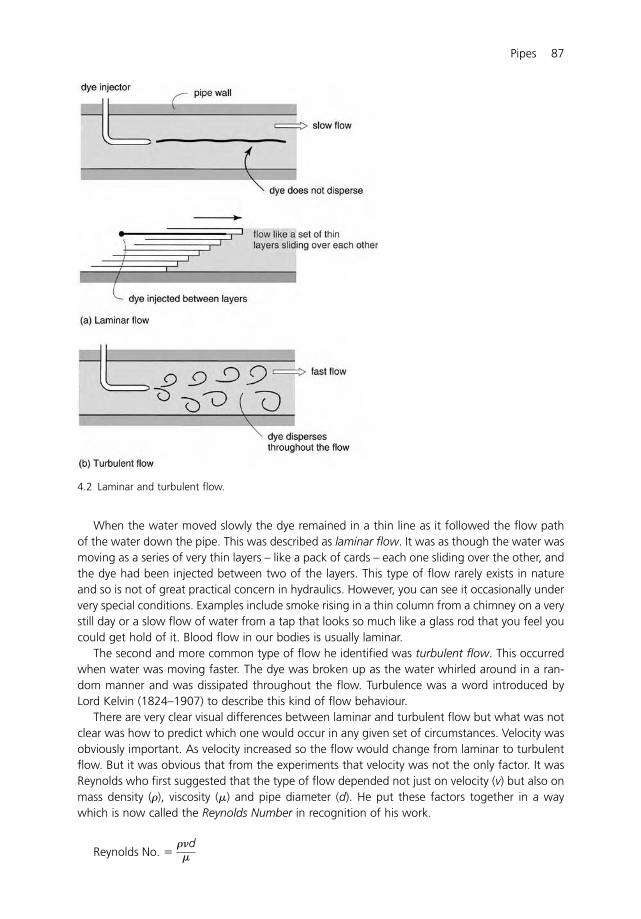
When the water moved slowly the dye remained in a thin line as it followed the flow pathof the water down the pipe. This was described as laminar flow. It was as though the water wasmoving as a series of very thin layers – like a pack of cards – each one sliding over the other, andthe dye had been injected between two of the layers. This type of flow rarely exists in natureand so is not of great practical concern in hydraulics. However, you can see it occasionally undervery special conditions. Examples include smoke rising in a thin column from a chimney on a verystill day or a slow flow of water from a tap that looks so much like a glass rod that you feel youcould get hold of it. Blood flow in our bodies is usually laminar.
The second and more common type of flow he identified was turbulent flow. This occurredwhen water was moving faster. The dye was broken up as the water whirled around in a ran-dom manner and was dissipated throughout the flow. Turbulence was a word introduced byLord Kelvin (1824–1907) to describe this kind of flow behaviour.
There are very clear visual differences between laminar and turbulent flow but what was notclear was how to predict which one would occur in any given set of circumstances. Velocity wasobviously important. As velocity increased so the flow would change from laminar to turbulentflow. But it was obvious that from the experiments that velocity was not the only factor. It wasReynolds who first suggested that the type of flow depended not just on velocity (v) but also onmass density (�), viscosity (�) and pipe diameter (d). He put these factors together in a waywhich is now called the Reynolds Number in recognition of his work.
Reynolds No. � ��d�
Pipes 87
4.2 Laminar and turbulent flow.
Note that Reynolds Number has no dimensions. All the dimensions cancel out. Reynoldsfound that he could use this number to reliably predict when laminar and turbulent flow wouldoccur.
R 2000 flow would always be laminarR � 4000 flow would always be turbulent
Between R � 2000 and 4000 he observed a very unstable zone as the flow seemed to jumpfrom laminar to turbulent and back again as if the flow could not decide which of the twoconditions it preferred. This is a zone to avoid as both the pressure and flow fluctuate widely inan uncontrolled manner.
Reynolds Number also shows just how important is viscosity in pipe flow. Low ReynoldsNumber (R 2000) means that viscosity (�) is large compared with the term �vd. So viscosity isimportant in laminar flow and cannot be ignored. High Reynolds Number (R � 4000) meansviscosity is small compared with the �vd term and so it follows that viscosity is less important inturbulent flow. This is the reason why engineers ignore the viscosity of water when designingpipes and channels as it has no material effect on the solution. Ignoring viscosity also greatlysimplifies pipeline design.
It has since been found that Reynolds Number is very useful in other ways besides telling usthe difference between laminar and turbulent flow. It is used extensively in hydraulic modelling(physical models – not mathematical models) for solving complex hydraulic problems. When aproblem cannot be solved using some formula, another approach is to construct a small-scalemodel in a laboratory and test it to see how it performs. The guideline for modelling pipesystems (or indeed any fully enclosed system) is to ensure that the Reynolds Number in themodel is similar to the Reynolds Number in the real situation. This ensures that the forces andvelocities are similar so that the model, as near as possible, produces similar results to those inthe real pipe systems.
Although it is useful to know that laminar flow exists it is not important in practicalhydraulics for designing pipes and channels and so only turbulent flow is considered in this text.Turbulent flow is very important to us in our daily lives. Indeed it would be difficult for us to liveif it was not for the mixing that takes place in turbulent flow which dilutes fluids. When webreathe out, the carbon dioxide from our lungs is dissipated into the surrounding air throughturbulent mixing. If it did not disperse in this way we would have to move our heads to avoidbreathing in the same gases as we had just breathed out. Car exhaust fumes are dispersed in asimilar way, otherwise we could be quickly poisoned by the intake of concentrated carbonmonoxide.
4.3.2 A formula for turbulent flow
Several formulae link energy loss with pipe size for turbulent flow but one of the most com-monly used today is that devised by Julius Weisbach (1806–1871) and Henry Darcy(1803–1858). It is often referred to as the Darcy–Weisbach equation:
where � is a friction factor; l is pipe length (m); v is velocity (m/s); g is gravity constant (9.81 m/s2)and d is pipe diameter (m).
hf �
� lv2
2gd
88 Pipes
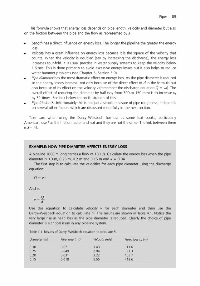
This formula shows that energy loss depends on pipe length, velocity and diameter but alsoon the friction between the pipe and the flow as represented by �:
� Length has a direct influence on energy loss. The longer the pipeline the greater the energyloss.
� Velocity has a great influence on energy loss because it is the square of the velocity thatcounts. When the velocity is doubled (say by increasing the discharge), the energy lossincreases four-fold. It is usual practice in water supply systems to keep the velocity below1.6 m/s. This is done primarily to avoid excessive energy losses but it also helps to reducewater hammer problems (see Chapter 5, Section 5.9).
� Pipe diameter has the most dramatic effect on energy loss. As the pipe diameter is reducedso the energy losses increase, not only because of the direct effect of d in the formula butalso because of its effect on the velocity v (remember the discharge equation Q � va). Theoverall effect of reducing the diameter by half (say from 300 to 150 mm) is to increase hf
by 32-times. See box below for an illustration of this.� Pipe friction λ Unfortunately this is not just a simple measure of pipe roughness; it depends
on several other factors which are discussed more fully in the next section.
Take care when using the Darcy–Weisbach formula as some text books, particularlyAmerican, use f as the friction factor and not and they are not the same. The link between themis �� 4f.
Pipes 89
EXAMPLE: HOW PIPE DIAMETER AFFECTS ENERGY LOSS
A pipeline 1000 m long carries a flow of 100 l/s. Calculate the energy loss when the pipediameter is 0.3 m, 0.25 m, 0.2 m and 0.15 m and � � 0.04.
The first step is to calculate the velocities for each pipe diameter using the dischargeequation:
Q � va
And so:
v �
Use this equation to calculate velocity v for each diameter and then use theDarcy–Weisbach equation to calculate hf. The results are shown in Table 4.1. Notice thevery large rise in head loss as the pipe diameter is reduced. Clearly the choice of pipediameter is a critical issue in any pipeline system.
Qa
Table 4.1 Results of Darcy–Weisbach equation to calculate hf.
Diameter (m) Pipe area (m2) Velocity (m/s) Head loss hf (m)
0.30 0.07 1.43 13.60.25 0.049 2.04 33.30.20 0.031 3.22 103.70.15 0.018 5.55 418.6
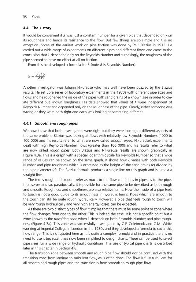
4.4 The � story
It would be convenient if � was just a constant number for a given pipe that depended only onits roughness and hence its resistance to the flow. But few things are so simple and � is noexception. Some of the earliest work on pipe friction was done by Paul Blazius in 1913. He carried out a wide range of experiments on different pipes and different flows and came to theconclusion that � depended only on the Reynolds Number and surprisingly, the roughness of thepipe seemed to have no effect at all on friction.
From this he developed a formula for � (note R is Reynolds Number):
Another investigator was Johann Nikuradse who may well have been puzzled by the Blaziusresults. He set up a series of laboratory experiments in the 1930s with different pipe sizes andflows and he roughened the inside of the pipes with sand grains of a known size in order to cre-ate different but known roughness. His data showed that values of � were independent ofReynolds Number and depended only on the roughness of the pipe. Clearly, either someone waswrong or they were both right and each was looking at something different.
4.4.1 Smooth and rough pipes
We now know that both investigators were right but they were looking at different aspects ofthe same problem. Blazius was looking at flows with relatively low Reynolds Numbers (4000 to100 000) and his results refer to what are now called smooth pipes. Nikuradse’s experimentsdealt with high Reynolds Number flows (greater than 100 000) and his results refer to whatare now called rough pipes. Both Blazius and Nikuradse results are shown graphically inFigure 4.3a. This is a graph with a special logarithmic scale for Reynolds Number so that a widerange of values can be shown on the same graph. It shows how � varies with both ReynoldsNumber and pipe roughness which is expressed as the height of the sand grains (k) divided bythe pipe diameter (d). The Blazius formula produces a single line on this graph and is almost astraight line.
The terms rough and smooth refer as much to the flow conditions in pipes as to the pipesthemselves and so, paradoxically, it is possible for the same pipe to be described as both roughand smooth. Roughness and smoothness are also relative terms. How the inside of a pipe feelsto touch is not a good guide to its smoothness in hydraulic terms. Pipes which are smooth tothe touch can still be quite rough hydraulically. However, a pipe that feels rough to touch willbe very rough hydraulically and very high energy losses can be expected.
As there are two distinct types of flow it implies that there must be some point or zone wherethe flow changes from one to the other. This is indeed the case. It is not a specific point but azone known as the transition zone when � depends on both Reynolds Number and pipe rough-ness (Figure 4.3a). This zone was successfully investigated by C.F. Colebrook and C.M. Whiteworking at Imperial College in London in the 1930s and they developed a formula to cover thisflow range. This is not quoted here as it is quite a complex formula and in practice there is noneed to use it because it has now been simplified to design charts. These can be used to selectpipe sizes for a wide range of hydraulic conditions. The use of typical pipe charts is describedlater in this chapter in Section 4.8.
The transition zone between smooth and rough pipe flow should not be confused with thetransition zone from laminar to turbulent flow, as is often done. The flow is fully turbulent forall smooth and rough pipes and the transition is from smooth to rough pipe flow.
� � 0.316R 0.25
90 Pipes
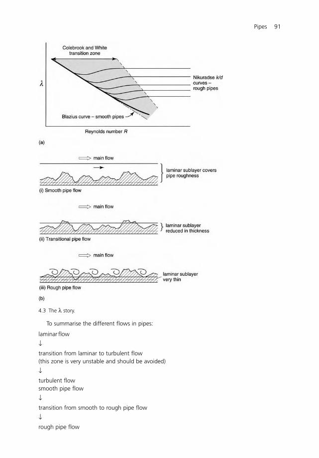
To summarise the different flows in pipes:
laminar flow
↓transition from laminar to turbulent flow(this zone is very unstable and should be avoided)
↓turbulent flowsmooth pipe flow
↓transition from smooth to rough pipe flow
↓rough pipe flow
Pipes 91
4.3 The λ story.
4.4.2 A physical explanation
Since those early experiments, modern scientific techniques have enabled investigators to lookmore closely at what happens close to a pipe wall. This has resulted in a physical explanationfor smooth and rough pipe flow (Figure 4.3b). Investigators have found that even when the flowis turbulent there exists a very thin layer of fluid – less than 1 mm thick – close to the boundarythat is laminar. This is called the laminar sub-layer. At low Reynolds Numbers the laminar sub-layeris at its thickest and completely covers the roughness of the pipe. The main flow is unaffected bythe boundary roughness and is influenced mainly by viscosity in the laminar sub-layer. It seems thatthe layer covers the roughness like a blanket and protects the flow from the pipe wall. This is thesmooth pipe flow that Blazius investigated. As Reynolds Number increases, the laminar sub-layerbecomes thinner and roughness elements start to protrude into the main flow. The flow is nowinfluenced both by viscosity and pipe roughness. This is the transition zone. As Reynolds Numberis further increased the sub-layer all but disappears and the roughness of the pipe wall takes overand dominates the friction. This is rough pipe flow which Nikuradse investigated.
Commercially manufactured pipes are not artificially roughened with sand like experimentalpipes, they are manufactured as smooth as possible to reduce energy losses. For this reason theytend to come within the transition zone where � varies with both Reynolds Number and piperoughness.
4.5 Hydraulic gradient
One way of showing energy losses in a pipeline is to use a diagram (Figure 4.4a). The totalenergy is shown as a line drawn along the pipe length and marked e—e—e. This line alwaysslopes downwards in the direction of the flow and demonstrates that energy is continually beinglost through friction. It connects the water surfaces in the two tanks. There is a small step at thedownstream tank to represent the energy loss at the outlet from the pipeline into the tank. Notethat the energy line is not necessarily parallel to the pipeline. The pipeline usually just followsthe natural ground surface profile.
Although total energy is of interest, pressure is more important because this determines howstrong the pipes must be to avoid bursts. For this reason a second line is drawn below the energyline, but parallel to it, to represent the pressure (pressure energy) and is marked h—h—h. Thisshows the pressure change along the pipeline. Imagine standpipes are attached to the pipe.Water would rise up to this line to represent the pressure head (Figure 4.4a). The differencebetween the two lines is the kinetic energy. Notice how both the energy line and the hydraulicgradient are straight lines. This shows that the rate of energy loss and the pressure loss are uni-form (at the same rate). The slope of the pressure line is called the hydraulic gradient. It is cal-culated as follows:
where hf is change in pressure (m); l is the pipe length over which the pressure change takesplace (m).
The hydraulic gradient has no dimensions as it comes from dividing a length in metres by ahead difference in metres. However, it is often expressed in terms of metres head per metre lengthof pipeline. As an example a hydraulic gradient of 0.02 means for every one metre of pipeline therewill be a pressure loss of 0.02 m. This may also be written as 0.02 m/m or as 2 m/100 m ofpipeline. This reduces the number of decimal places that must be dealt with and means that for
hydraulic gradient � hf
l
92 Pipes
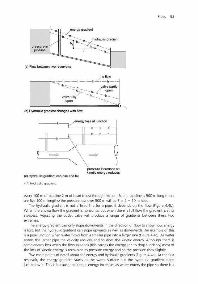
every 100 m of pipeline 2 m of head is lost through friction. So if a pipeline is 500 m long (thereare five 100 m lengths) the pressure loss over 500 m will be 5 � 2 � 10 m head.
The hydraulic gradient is not a fixed line for a pipe; it depends on the flow (Figure 4.4b).When there is no flow the gradient is horizontal but when there is full flow the gradient is at itssteepest. Adjusting the outlet valve will produce a range of gradients between these twoextremes.
The energy gradient can only slope downwards in the direction of flow to show how energyis lost, but the hydraulic gradient can slope upwards as well as downwards. An example of thisis a pipe junction when water flows from a smaller pipe into a larger one (Figure 4.4c). As waterenters the larger pipe the velocity reduces and so does the kinetic energy. Although there issome energy loss when the flow expands (this causes the energy line to drop suddenly) most ofthe loss of kinetic energy is recovered as pressure energy and so the pressure rises slightly.
Two more points of detail about the energy and hydraulic gradients (Figure 4.4a). At the firstreservoir, the energy gradient starts at the water surface but the hydraulic gradient startsjust below it. This is because the kinetic energy increases as water enters the pipe so there is a
Pipes 93
4.4 Hydraulic gradient.
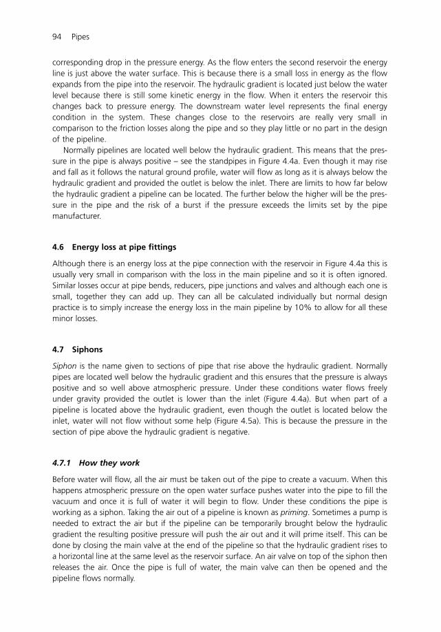
corresponding drop in the pressure energy. As the flow enters the second reservoir the energyline is just above the water surface. This is because there is a small loss in energy as the flowexpands from the pipe into the reservoir. The hydraulic gradient is located just below the waterlevel because there is still some kinetic energy in the flow. When it enters the reservoir thischanges back to pressure energy. The downstream water level represents the final energycondition in the system. These changes close to the reservoirs are really very small incomparison to the friction losses along the pipe and so they play little or no part in the designof the pipeline.
Normally pipelines are located well below the hydraulic gradient. This means that the pres-sure in the pipe is always positive – see the standpipes in Figure 4.4a. Even though it may riseand fall as it follows the natural ground profile, water will flow as long as it is always below thehydraulic gradient and provided the outlet is below the inlet. There are limits to how far belowthe hydraulic gradient a pipeline can be located. The further below the higher will be the pres-sure in the pipe and the risk of a burst if the pressure exceeds the limits set by the pipemanufacturer.
4.6 Energy loss at pipe fittings
Although there is an energy loss at the pipe connection with the reservoir in Figure 4.4a this isusually very small in comparison with the loss in the main pipeline and so it is often ignored.Similar losses occur at pipe bends, reducers, pipe junctions and valves and although each one issmall, together they can add up. They can all be calculated individually but normal designpractice is to simply increase the energy loss in the main pipeline by 10% to allow for all theseminor losses.
4.7 Siphons
Siphon is the name given to sections of pipe that rise above the hydraulic gradient. Normallypipes are located well below the hydraulic gradient and this ensures that the pressure is alwayspositive and so well above atmospheric pressure. Under these conditions water flows freelyunder gravity provided the outlet is lower than the inlet (Figure 4.4a). But when part of apipeline is located above the hydraulic gradient, even though the outlet is located below theinlet, water will not flow without some help (Figure 4.5a). This is because the pressure in thesection of pipe above the hydraulic gradient is negative.
4.7.1 How they work
Before water will flow, all the air must be taken out of the pipe to create a vacuum. When thishappens atmospheric pressure on the open water surface pushes water into the pipe to fill thevacuum and once it is full of water it will begin to flow. Under these conditions the pipe isworking as a siphon. Taking the air out of a pipeline is known as priming. Sometimes a pump isneeded to extract the air but if the pipeline can be temporarily brought below the hydraulicgradient the resulting positive pressure will push the air out and it will prime itself. This can bedone by closing the main valve at the end of the pipeline so that the hydraulic gradient rises toa horizontal line at the same level as the reservoir surface. An air valve on top of the siphon thenreleases the air. Once the pipe is full of water, the main valve can then be opened and thepipeline flows normally.
94 Pipes
Even pipelines that normally operate under positive pressures have air valves. These releaseair which accumulates at high spots along the line. So it is good practice to include an air valveat such locations. They can be automatic valves or just simple gate valves that are openedmanually occasionally to release air.
It can sometimes be difficult to spot an air valve that is above the hydraulic gradient and thiscan lead to problems. An engineer visiting a remote farm saw what he thought was a simplegated air valve on a high spot on a pipeline supplying the farm with water. Air does tend toaccumulate over time and can restrict the flow. So he thought he would do the farmer a favourand open the valve to bleed off any air that had accumulated. After a while he realised that thehissing sound was not air escaping from the pipe but air rushing in. The pipe was in fact abovethe hydraulic gradient and was working as a siphon at that point and the valve was only thereto let air out during the priming process. The pressure inside the pipe was in fact negative andso when he opened the valve air was sucked and this de-primed the siphon. Realising hismistake he quickly closed the valve and went on down to the farmhouse. The farmer was most
Pipes 95
4.5 Siphons.
upset. What a coincidence – just as a water engineer had arrived, his water supply had suddenlystopped and an engineer was on hand to fix it for him!
If your car ever runs out of petrol a siphon can be a useful means of taking some fuel froma neighbour’s tank. Insert a flexible small diameter tube into the tank and suck out all the air(making sure not to get a mouthful of petrol). When the petrol begins to flow catch it in acontainer and then transfer it to your car. Make sure that the outlet is lower than the liquid levelin the tank otherwise the siphon will not work.
Another very practical use for siphons is to detect leakage in domestic water mains(sometimes called rising mains) from the supply outside in the street to a house (Figure 4.5b).This can be important for those on a water meter who pay high prices for their water. A leakypipe in this situation would be very costly. The main valve to the house must first be closed. Thenseal the cold water tap inside the house by immersing the outlet in a pan of water and openingthe tap. If there is any leakage in the main pipe then water will be siphoned back out of the paninto the main. The rate of flow will indicate the extent of the leakage.
Siphons can be very useful in situations where the land topography is undulatingbetween a reservoir and the water users. It is always preferable to locate a pipe below thehydraulic gradient by putting it in a deep trench but this may not always be practicable. Insituations where siphoning is unavoidable the pipeline must not be more than 7 m abovethe hydraulic grade line. Remember atmospheric pressure drives a siphon and the absolutelimit is 10 m head of water. So 7 m is a safe practical limit. When pipelines are located inmountainous regions the limit needs to be lower than this due to the reduced atmosphericpressure.
The pressure inside a working siphon is less than atmospheric pressure and so it is negativewhen referred to as a gauge pressure (measured above or below atmospheric pressure asthe datum), for example, a �7 m head. Sometimes siphon pressures are quoted as absolutepressures (measured above vacuum pressure as the datum). So �7 m gauge pressure is the sameas �3 m absolute pressure. This is calculated as follows:
gauge pressure � �7 m headabsolute pressure � atmospheric pressure � gauge pressure
� 10 � 7 � 3 m head absolute
4.8 Selecting pipe sizes in practice
The development of � as a pipe roughness coefficient is an interesting story and this nicelyleads into the use of the Darcy–Weisbach formula for linking energy loss with the various pipeparameters. There are several examples using this formula in the boxes and they demon-strate well the effects of pipe length, diameter and velocity on energy loss. So it is a usefullearning tool.
Engineers in different industries and in different countries have also used other formulaeoften developed empirically to fit their particular circumstances. But these are gradually beingabandoned and replaced by the Colebrook-White formula which accurately deals with mostcommercially available pipes. The task of using the formula, which is a rather complicated one,is made simple by the fact that it is now available as a set of design charts (Figure 4.6). The chartsare also easier to use because discharge can be related directly to pipe diameter whereasDarcy–Weisbach formula only links to velocity and so requires an extra step (continuity equation)to get to discharge.
The boxes provide examples of the use of Darcy–Weisbach formula and design charts basedon Colebrook-White formula.
96 Pipes
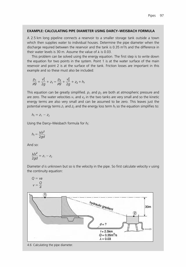
Pipes 97
EXAMPLE: CALCULATING PIPE DIAMETER USING DARCY–WEISBACH FORMULA
A 2.5 km long pipeline connects a reservoir to a smaller storage tank outside a townwhich then supplies water to individual houses. Determine the pipe diameter when thedischarge required between the reservoir and the tank is 0.35 m3/s and the difference intheir water levels is 30 m. Assume the value of � is 0.03.
This problem can be solved using the energy equation. The first step is to write downthe equation for two points in the system. Point 1 is at the water surface of the mainreservoir and point 2 is at the surface of the tank. Friction losses are important in thisexample and so these must also be included:
This equation can be greatly simplified. p1 and p2 are both at atmospheric pressure andare zero. The water velocities v1 and v2 in the two tanks are very small and so the kineticenergy terms are also very small and can be assumed to be zero. This leaves just thepotential energy terms z1 and z2 and the energy loss term hf so the equation simplifies to:
hf � z1 � z2
Using the Darcy–Weisbach formula for hf:
And so:
Diameter d is unknown but so is the velocity in the pipe. So first calculate velocity v usingthe continuity equation:
Q � va
v � Qa
�lv2
2gd � z1 � z2
hf � �lv2
2gd
p1
�g � v2
1
2g � z1 �
p2
�g � v2
2
2g � z2 � hf
4.6 Calculating the pipe diameter.
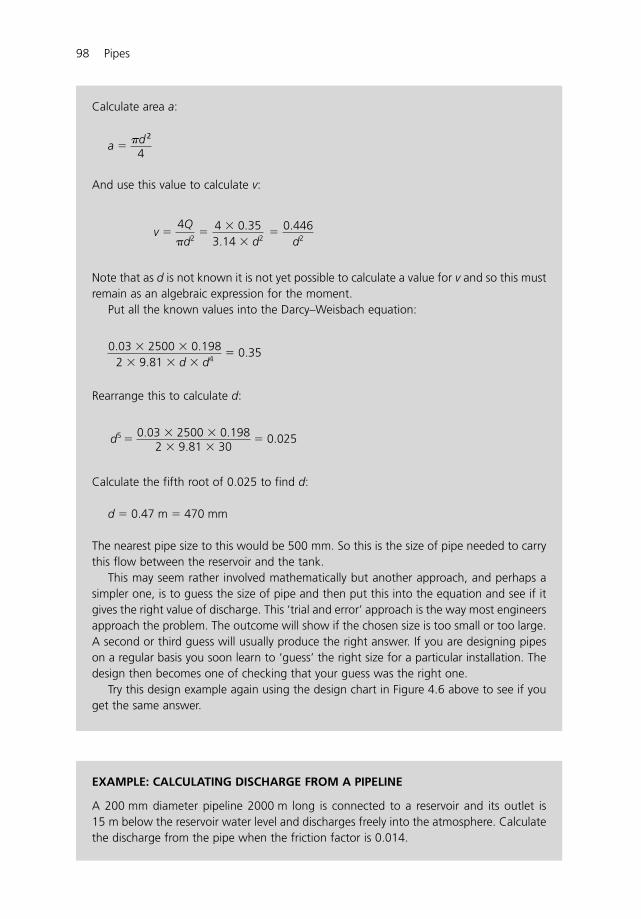
98 Pipes
Calculate area a:
And use this value to calculate v:
�
Note that as d is not known it is not yet possible to calculate a value for v and so this mustremain as an algebraic expression for the moment.
Put all the known values into the Darcy–Weisbach equation:
Rearrange this to calculate d:
Calculate the fifth root of 0.025 to find d:
d � 0.47 m � 470 mm
The nearest pipe size to this would be 500 mm. So this is the size of pipe needed to carrythis flow between the reservoir and the tank.
This may seem rather involved mathematically but another approach, and perhaps asimpler one, is to guess the size of pipe and then put this into the equation and see if itgives the right value of discharge. This ‘trial and error’ approach is the way most engineersapproach the problem. The outcome will show if the chosen size is too small or too large.A second or third guess will usually produce the right answer. If you are designing pipeson a regular basis you soon learn to ‘guess’ the right size for a particular installation. Thedesign then becomes one of checking that your guess was the right one.
Try this design example again using the design chart in Figure 4.6 above to see if youget the same answer.
d5 � 0.03 � 2500 � 0.1982 � 9.81 � 30
� 0.025
0.03 � 2500 � 0.1982 � 9.81 � d � d4
� 0.35
4 � 0.353.14 � d2
� 0.446d2
v � 4Q
�d2
a � �d 2
4
EXAMPLE: CALCULATING DISCHARGE FROM A PIPELINE
A 200 mm diameter pipeline 2000 m long is connected to a reservoir and its outlet is15 m below the reservoir water level and discharges freely into the atmosphere. Calculatethe discharge from the pipe when the friction factor is 0.014.
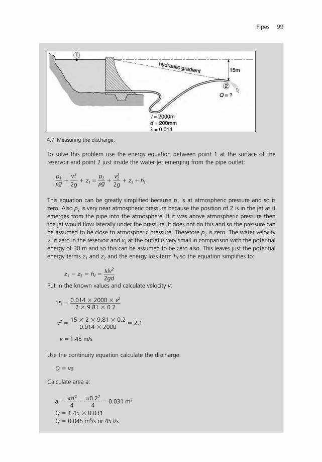
Pipes 99
To solve this problem use the energy equation between point 1 at the surface of thereservoir and point 2 just inside the water jet emerging from the pipe outlet:
This equation can be greatly simplified because p1 is at atmospheric pressure and so iszero. Also p2 is very near atmospheric pressure because the position of 2 is in the jet as itemerges from the pipe into the atmosphere. If it was above atmospheric pressure thenthe jet would flow laterally under the pressure. It does not do this and so the pressure canbe assumed to be close to atmospheric pressure. Therefore p2 is zero. The water velocityv1 is zero in the reservoir and v2 at the outlet is very small in comparison with the potentialenergy of 30 m and so this can be assumed to be zero also. This leaves just the potentialenergy terms z1 and z2 and the energy loss term hf so the equation simplifies to:
z1 � z2 � hf �
Put in the known values and calculate velocity v:
15 �
v2 � � 2.1
v � 1.45 m/s
Use the continuity equation calculate the discharge:
Q � va
Calculate area a:
a � � � 0.031 m2
Q � 1.45 � 0.031Q � 0.045 m3/s or 45 l/s
�0.22
4�d 2
4
15 � 2 � 9.81 � 0.20.014 � 2000
0.014 � 2000 � v2
2 � 9.81 � 0.2
�lv2
2gd
p1
�g � v 2
1
2g � z1 �
p2
�g � v2
2
2g � z2 � hf
4.7 Measuring the discharge.
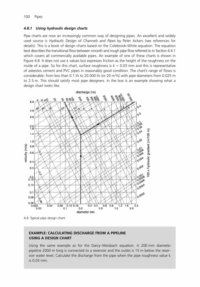
4.8.1 Using hydraulic design charts
Pipe charts are now an increasingly common way of designing pipes. An excellent and widelyused source is Hydraulic Design of Channels and Pipes by Peter Ackers (see references fordetails). This is a book of design charts based on the Colebrook-White equation. The equationbest describes the transitional flow between smooth and rough pipe flow referred to in Section 4.4.1which covers all commercially available pipes. An example of one of these charts is shown inFigure 4.8. It does not use � values but expresses friction as the height of the roughness on theinside of a pipe. So for this chart, surface roughness is k � 0.03 mm and this is representativeof asbestos cement and PVC pipes in reasonably good condition. The chart’s range of flows isconsiderable; from less than 0.1 l/s to 20 000 l/s (or 20 m3/s) with pipe diameters from 0.025 mto 2.5 m. This should satisfy most pipe designers. In the box is an example showing what adesign chart looks like.
100 Pipes
EXAMPLE: CALCULATING DISCHARGE FROM A PIPELINE USING A DESIGN CHART
Using the same example as for the Darcy–Weisbach equation. A 200 mm diameterpipeline 2000 m long is connected to a reservoir and the outlet is 15 m below the reser-voir water level. Calculate the discharge from the pipe when the pipe roughness value kis 0.03 mm.
4.8 Typical pipe design chart.
Pipes 101
There are four important practical points to note from the examples.The first point refers to the first worked example which showed how mathematically
cumbersome it can be to determine the diameter by calculation. The easier way is to do whatmost engineers do; they guess the diameter and then check by calculation that their chosenpipe is the right one. This might seem a strange way of approaching a problem but it is quitecommon in engineering. It always helps to know approximately the answer to a problem beforebeginning to solve it. An experienced engineer usually knows what answer to expect; the cal-culation then becomes just a way of confirming this. (This is one of the basic unwritten laws ofengineering – that you need to know the answer to the problem before you begin so that youknow that you have the right answer when you get there.) This foresight is important becausewhen you calculate a pipe diameter how will you know that you have arrived at the rightanswer? There will not be any answers available to the real problems in the field as there arein this text book and there may not be anyone around to ask if it is the right answer. You needto know that you have the right answer and this comes largely from experience of similar designproblems. New designers are unlikely to have this experience, but they have to start some-where and one way is to rely initially on the experience of others and to learn from them. Thisis the apprenticeship that all engineers go through to gain experience and become competentdesigners.
The second point to note is that there is no one unique pipe diameter that must be used inany given situation. If, for example, calculations show that a 100 mm pipe is sufficient then anypipe larger than this will also carry the flow. The question of which one is the most acceptableis usually determined by several design criteria. One is that the velocity should not exceed1.6 m/s. Another might be a limit on the head that can be lost through friction. A third could bea limit on the pipe sizes available. There are only certain standard sizes which are manufacturedand not all these may be readily available in some countries. A final deciding factor is cost – whichpipe is the cheapest to buy and to operate?
The third point to consider is the value for pipe roughness. It is easy to choose the value fora new pipe but how long will it be before the roughness increases? What will the value be in,
The design chart uses the hydraulic gradient to show the rate of head loss in a pipeline.So the first step is to calculate the hydraulic gradient from the information given above.The pipe is 2000 m long and the head loss from the reservoir to the pipe outlet is 15 m so:
hydraulic gradient � � � 0.0075
or � 0.75 m/100 m
Using the chart locate the intersection of the lines for a hydraulic gradient of0.75 m/100 m and a diameter of 200 mm. This locates the discharge line and the valueof the discharge:
Q � 0.045 m3/s or 45 l/s
Note that the chart can also be used in reverse to determine the diameter of a pipe andhead loss for a given discharge.
152000
hl
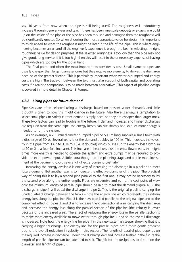
say, 10 years from now when the pipe is still being used? The roughness will undoubtedlyincrease through general wear and tear. If there has been lime scale deposits or algae slime buildup on the inside of the pipe or the pipe has been misused and damaged then the roughness willbe significantly greater. So when choosing the most appropriate value for design it is importantto think ahead to what the roughness might be later in the life of the pipe. This is where engi-neering becomes an art and all the engineer’s experience is brought to bear in selecting the rightroughness value for design purposes. If the selected roughness is too low then the pipe may notgive good, long service. If it is too high then this will result in the unnecessary expense of havingpipes which are too big for the job in hand.
The final point, and often the most important to consider, is cost. Small diameter pipes areusually cheaper than larger diameter ones but they require more energy to deliver the dischargebecause of the greater friction. This is particularly important when water is pumped and energycosts are high. The trade-off between the two must take account of both capital and operatingcosts if a realistic comparison is to be made between alternatives. This aspect of pipeline designis covered in more detail in Chapter 8 Pumps.
4.8.2 Sizing pipes for future demand
Pipe sizes are often selected using a discharge based on present water demands and littlethought is given to how this might change in the future. Also there is always a temptation toselect small pipes to satisfy current demand simply because they are cheaper than larger ones.These two factors can lead to trouble in the future. If demand increases and higher dischargesare required from the same pipe, the energy losses can rise sharply and so a lot more energy isneeded to run the system.
As an example, a 200 mm diameter pumped pipeline 500 m long supplies a small town witha discharge of 50 l/s. Several years later the demand doubles to 100 l/s. This increases the veloc-ity in the pipe from 1.67 to 3.34 m/s (i.e. it doubles) which pushes up the energy loss from 5 mto 20 m (i.e. a four-fold increase). This increase in head loss plus the extra flow means that eighttimes more energy is needed to operate the system and extra pumps may be required to pro-vide the extra power input. A little extra thought at the planning stage and a little more invest-ment at the beginning could save a lot of extra pumping cost later.
Increasing the energy available is one way of increasing the discharge in a pipeline to meetfuture demand. But another way is to increase the effective diameter of the pipe. The practicalway of doing this is to lay a second pipe parallel to the first one. It may not be necessary to laythe second pipe along the entire length. Pipes are expensive and so from a cost point of viewonly the minimum length of parallel pipe should be laid to meet the demand (Figure 4.9). Thedischarge in pipe 1 will equal the discharge in pipe 2. This is the original pipeline carrying the(inadequate) discharge between the tanks – note the energy line which represents the uniformenergy loss along the pipeline. Pipe 3 is the new pipe laid parallel to the original pipe and so thecombined effect of pipes 2 and 3 is to increase the cross-sectional area carrying the dischargeand decrease the energy loss along the parallel section of the pipeline (the velocity is lowerbecause of the increased area). The effect of reducing the energy loss in the parallel section isto make more energy available to move water through pipeline 1 and so the overall dischargeis increased. Note how the energy line for pipe 1 in the new system is steeper showing that it iscarrying a higher discharge. The energy line for the parallel pipes has a more gentle gradientdue to the overall reduction in velocity in this section. The length of parallel pipe depends onthe required increase in discharge. Should the discharge demand increase further in the future thelength of parallel pipeline can be extended to suit. The job for the designer is to decide on thediameter and length of pipe 3.
102 Pipes
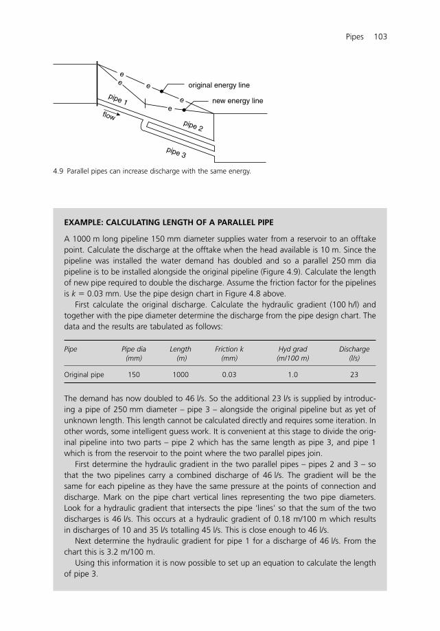
Pipes 103
pipe 1
ee
e
e
pipe 2
e
pipe 3
new energy line
flow
original energy line
4.9 Parallel pipes can increase discharge with the same energy.
EXAMPLE: CALCULATING LENGTH OF A PARALLEL PIPE
A 1000 m long pipeline 150 mm diameter supplies water from a reservoir to an offtakepoint. Calculate the discharge at the offtake when the head available is 10 m. Since thepipeline was installed the water demand has doubled and so a parallel 250 mm diapipeline is to be installed alongside the original pipeline (Figure 4.9). Calculate the lengthof new pipe required to double the discharge. Assume the friction factor for the pipelinesis k � 0.03 mm. Use the pipe design chart in Figure 4.8 above.
First calculate the original discharge. Calculate the hydraulic gradient (100 h/l) andtogether with the pipe diameter determine the discharge from the pipe design chart. Thedata and the results are tabulated as follows:
Pipe Pipe dia Length Friction k Hyd grad Discharge(mm) (m) (mm) (m/100 m) (l/s)
Original pipe 150 1000 0.03 1.0 23
The demand has now doubled to 46 l/s. So the additional 23 l/s is supplied by introduc-ing a pipe of 250 mm diameter – pipe 3 – alongside the original pipeline but as yet ofunknown length. This length cannot be calculated directly and requires some iteration. Inother words, some intelligent guess work. It is convenient at this stage to divide the orig-inal pipeline into two parts – pipe 2 which has the same length as pipe 3, and pipe 1which is from the reservoir to the point where the two parallel pipes join.
First determine the hydraulic gradient in the two parallel pipes – pipes 2 and 3 – sothat the two pipelines carry a combined discharge of 46 l/s. The gradient will be thesame for each pipeIine as they have the same pressure at the points of connection anddischarge. Mark on the pipe chart vertical lines representing the two pipe diameters.Look for a hydraulic gradient that intersects the pipe ‘lines’ so that the sum of the twodischarges is 46 l/s. This occurs at a hydraulic gradient of 0.18 m/100 m which resultsin discharges of 10 and 35 l/s totalling 45 l/s. This is close enough to 46 l/s.
Next determine the hydraulic gradient for pipe 1 for a discharge of 46 l/s. From thechart this is 3.2 m/100 m.
Using this information it is now possible to set up an equation to calculate the lengthof pipe 3.
104 Pipes
The sum of the head loss in pipes 1 and 3 (remember the loss in pipe 3 will be thesame as pipe 2) is 10 m. So:
h1 � h3 � 10 m
Now:
Similarly:
So:
Both L1 and L3 are unknown. So to ‘eliminate’ one of the unknowns substitute for L1 interms of L3:
L1 � 1000 – L3
Substitute this into the above equation:
� 10
(1000 – L3) 3.2 � 0.18L3 � 1000
3200 – 3.2L3 � 0.18L3 � 1000
3.38L3 � 2200
L3 � � 650 m
So the length of pipe 3 is 650 m. This is also the length of pipe 2. Pipe 1 will be 350 m.The following table summarises the results:
Pipe Pipe dia (mm) Friction k (mm) Hyd grad (m/100 m) Discharge (l/s) Length (m)
Pipe 1 150 0.03 3.20 46 350Pipe 2 150 0.03 0.18 10 650Pipe 3 250 0.03 0.18 35 650
This is one example where using a formula makes the problem easier to solve as it avoidsthe iterative approach. Try to solve the problem using the Darcy–Weisbach formula andthe continuity equation with a value of � � 0.04 for the pipes.
22003.38
(1000 � L3) � 3.2100
�
L3
�
0.18100
L1
�
3.2100
� L3
�
0.18100
� 10
h3 � L3
�
0.18100
h1 � L1
�
3.2100
100h1
L1 � hydraulic gradient � 3.2
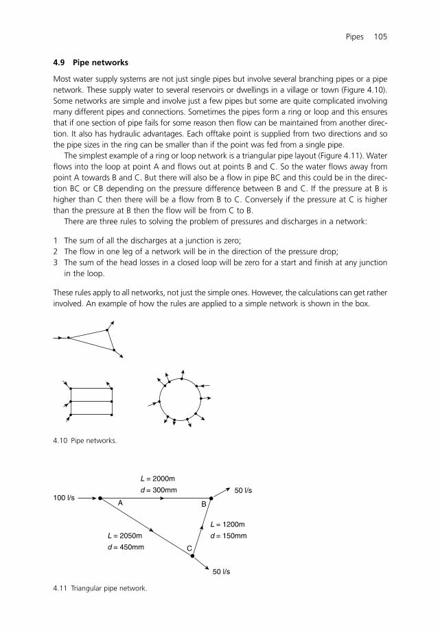
Pipes 105
4.9 Pipe networks
Most water supply systems are not just single pipes but involve several branching pipes or a pipenetwork. These supply water to several reservoirs or dwellings in a village or town (Figure 4.10).Some networks are simple and involve just a few pipes but some are quite complicated involvingmany different pipes and connections. Sometimes the pipes form a ring or loop and this ensuresthat if one section of pipe fails for some reason then flow can be maintained from another direc-tion. It also has hydraulic advantages. Each offtake point is supplied from two directions and sothe pipe sizes in the ring can be smaller than if the point was fed from a single pipe.
The simplest example of a ring or loop network is a triangular pipe layout (Figure 4.11). Waterflows into the loop at point A and flows out at points B and C. So the water flows away frompoint A towards B and C. But there will also be a flow in pipe BC and this could be in the direc-tion BC or CB depending on the pressure difference between B and C. If the pressure at B ishigher than C then there will be a flow from B to C. Conversely if the pressure at C is higherthan the pressure at B then the flow will be from C to B.
There are three rules to solving the problem of pressures and discharges in a network:
1 The sum of all the discharges at a junction is zero;2 The flow in one leg of a network will be in the direction of the pressure drop;3 The sum of the head losses in a closed loop will be zero for a start and finish at any junction
in the loop.
These rules apply to all networks, not just the simple ones. However, the calculations can get ratherinvolved. An example of how the rules are applied to a simple network is shown in the box.
4.10 Pipe networks.
50 l/s
100 l/s50 l/s
L = 1200m
d = 150mmL = 2050m
d = 450mm
L = 2000m
A B
C
d = 300mm
4.11 Triangular pipe network.
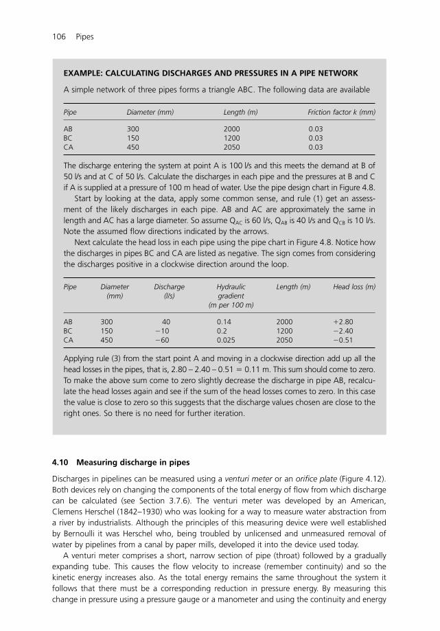
4.10 Measuring discharge in pipes
Discharges in pipelines can be measured using a venturi meter or an orifice plate (Figure 4.12).Both devices rely on changing the components of the total energy of flow from which dischargecan be calculated (see Section 3.7.6). The venturi meter was developed by an American,Clemens Herschel (1842–1930) who was looking for a way to measure water abstraction froma river by industrialists. Although the principles of this measuring device were well establishedby Bernoulli it was Herschel who, being troubled by unlicensed and unmeasured removal ofwater by pipelines from a canal by paper mills, developed it into the device used today.
A venturi meter comprises a short, narrow section of pipe (throat) followed by a graduallyexpanding tube. This causes the flow velocity to increase (remember continuity) and so thekinetic energy increases also. As the total energy remains the same throughout the system itfollows that there must be a corresponding reduction in pressure energy. By measuring thischange in pressure using a pressure gauge or a manometer and using the continuity and energy
106 Pipes
EXAMPLE: CALCULATING DISCHARGES AND PRESSURES IN A PIPE NETWORK
A simple network of three pipes forms a triangle ABC. The following data are available
Pipe Diameter (mm) Length (m) Friction factor k (mm)
AB 300 2000 0.03BC 150 1200 0.03CA 450 2050 0.03
The discharge entering the system at point A is 100 l/s and this meets the demand at B of50 l/s and at C of 50 l/s. Calculate the discharges in each pipe and the pressures at B and Cif A is supplied at a pressure of 100 m head of water. Use the pipe design chart in Figure 4.8.
Start by looking at the data, apply some common sense, and rule (1) get an assess-ment of the likely discharges in each pipe. AB and AC are approximately the same inlength and AC has a large diameter. So assume QAC is 60 l/s, QAB is 40 l/s and QCB is 10 l/s.Note the assumed flow directions indicated by the arrows.
Next calculate the head loss in each pipe using the pipe chart in Figure 4.8. Notice howthe discharges in pipes BC and CA are listed as negative. The sign comes from consideringthe discharges positive in a clockwise direction around the loop.
Pipe Diameter Discharge Hydraulic Length (m) Head loss (m)(mm) (l/s) gradient
(m per 100 m)
AB 300 40 0.14 2000 �2.80BC 150 �10 0.2 1200 �2.40CA 450 �60 0.025 2050 �0.51
Applying rule (3) from the start point A and moving in a clockwise direction add up all thehead losses in the pipes, that is, 2.80 – 2.40 – 0.51 � 0.11 m. This sum should come to zero.To make the above sum come to zero slightly decrease the discharge in pipe AB, recalcu-late the head losses again and see if the sum of the head losses comes to zero. In this casethe value is close to zero so this suggests that the discharge values chosen are close to theright ones. So there is no need for further iteration.
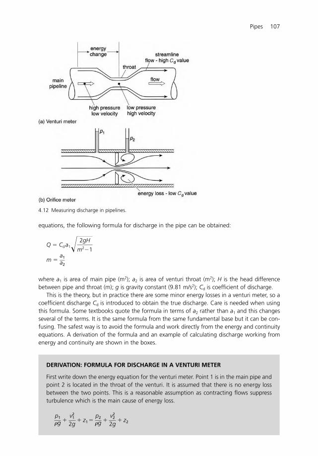
Pipes 107
equations, the following formula for discharge in the pipe can be obtained:
where a1 is area of main pipe (m2); a2 is area of venturi throat (m2); H is the head differencebetween pipe and throat (m); g is gravity constant (9.81 m/s2); Cd is coefficient of discharge.
This is the theory, but in practice there are some minor energy losses in a venturi meter, so acoefficient discharge Cd is introduced to obtain the true discharge. Care is needed when usingthis formula. Some textbooks quote the formula in terms of a2 rather than a1 and this changesseveral of the terms. It is the same formula from the same fundamental base but it can be con-fusing. The safest way is to avoid the formula and work directly from the energy and continuityequations. A derivation of the formula and an example of calculating discharge working fromenergy and continuity are shown in the boxes.
m � a1
a2
Q � Cda1� 2gH
m2�1
4.12 Measuring discharge in pipelines.
DERIVATION: FORMULA FOR DISCHARGE IN A VENTURI METER
First write down the energy equation for the venturi meter. Point 1 is in the main pipe andpoint 2 is located in the throat of the venturi. It is assumed that there is no energy lossbetween the two points. This is a reasonable assumption as contracting flows suppressturbulence which is the main cause of energy loss.
p1
�g �
v21
2g � z1
�
p2
�g �
v22
2g � z2
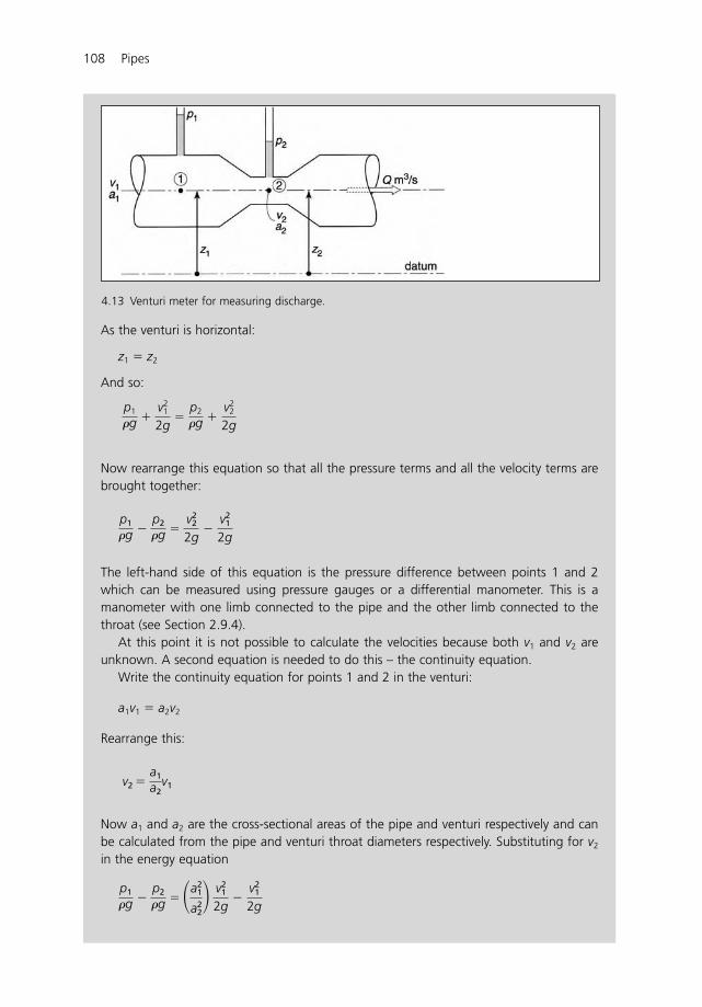
108 Pipes
As the venturi is horizontal:
z1 � z2
And so:
Now rearrange this equation so that all the pressure terms and all the velocity terms arebrought together:
The left-hand side of this equation is the pressure difference between points 1 and 2which can be measured using pressure gauges or a differential manometer. This is amanometer with one limb connected to the pipe and the other limb connected to thethroat (see Section 2.9.4).
At this point it is not possible to calculate the velocities because both v1 and v2 areunknown. A second equation is needed to do this – the continuity equation.
Write the continuity equation for points 1 and 2 in the venturi:
a1v1 � a2v2
Rearrange this:
Now a1 and a2 are the cross-sectional areas of the pipe and venturi respectively and canbe calculated from the pipe and venturi throat diameters respectively. Substituting for v2
in the energy equation
p1
�g � p2
�g � �a21
a22�
v21
2g �
v21
2g
v2 � a1
a2v1
p1
�g � p2
�g � v2
2
2g �
v21
2g
p1
�g � v2
1
2g �
p2
�g � v2
2
2g
4.13 Venturi meter for measuring discharge.
Pipes 109
In the case of the venturi meter Cd � 0.97 which means that the energy losses are small and theenergy theory works very well (Cd � 1.0 would mean the theory was perfect). For orifice platesthe same theory and formula can be used but the value of Cd is quite different at Cd � 0.6. Thetheory is not so good for this case because there is a lot of energy loss (Figure 4.12b). The wateris not channelled smoothly from one section to another as in the venturi but is forced to makeabrupt changes as it passes through the orifice and expands downstream. Such abruptnesscauses a lot of turbulence which results in energy loss. (The Cd value is similar to that for orificeflow from a tank – see Section 3.6.3.)
Put:
where H is the difference in head between the pipe (point 1) and the venturi throat point 2)
Rearrange the equation for v1
Use the continuity equation to calculate discharge:
Q � a1v1
And so:
Put:
And so:
Introduce a coefficient of discharge Cd:
Q � Cda1� 2gH
m2�1
Q � a1� 2gH
m2�1
m � a1
a2
Q � �2gH � a1a2
�a21�a2
2 �
v1 � �2gH � a2
�a21�a2
2 �
H � p1
�g � p2
�g
p1
�g � p2
�g � v2
1
2g �a2
1�a22
a22�
110 Pipes
EXAMPLE: CALCULATING DISCHARGE USING A VENTURI METER
A 120 mm diameter venturi meter is installed in a 250 mm diameter pipeline to measuredischarge. Calculate the discharge when the pressure difference between the pipe andthe venturi throat is 2.5 m of head of water and Cd is 0.97.
Although there is a formula for discharge it can be helpful to work from first princi-ples. Not only does this reinforce the principle but it also avoids possible errors in using arather involved formula which can easily be misquoted. So this example is worked fromthe energy and continuity equations.
First step write down the energy equation:
As the venturi is horizontal:
z1 � z2
And so:
Now rearrange this equation so that all the pressure terms and all the velocity terms arebrought together:
But:
Remember that the pressure terms are in m head of water and it is the difference that isimportant and not the individual pressures:And so:
It is not possible to solve this equation directly as both v1 and v2 are unknown. So use con-tinuity to obtain another equation for v1 and v2:
a1v1 � a2v2
Rearrange this:
Next step calculate the areas a1 and a2.
v2 � a1
a2 v1
v22
2g �
v21
2g � 2.5 m
p1
�g � p2
�g � 2.5 m
p1
�g � p2
�g � v2
2
2g �
v21
2g
p1
�g � v2
1
2g �
p2
�g � v2
2
2g
p1
�g � v2
1
2g � z1 �
p2
�g � v2
2
2g � z2
Pipes 111
Area of pipe:
Area of venturi:
Substitute this value for v2 in the energy equation:
20.7 � 2.5 � 2 � 9.81 � 49.05
Calculate Q:
Q � Cd v1 a1
� 0.97 � 1.57 � 0.05Q � 0.076 m3/s
v1 ��49.0519.7
�1.57 m/s
v21 � v2
1
4.552v21
2g �
v21
2g � 2.5 m
v2 � 0.050.011
v1 � 4.55 v1
a2 � �d2
2
4 � �0.122
4 � 0.011 m2
a1 � �d1
2
4 � �0.252
4 � 0.05 m2
EXAMPLE: CALCULATING THE FORCE ON A NOZZLE
A 100 mm diameter fire hose discharges 15 l/s from a 50 mm diameter nozzle. Calculatethe force on the nozzle.
To solve this problem all three hydraulic equations are needed; energy, continuity andmomentum. The energy and continuity equations are needed to calculate the pressure inthe 100 mm pipe and momentum is then used to calculate the force on the nozzle.
4.11 Momentum in pipes
The momentum equation is used in pipe flow to calculate forces on pipe fittings such as noz-zles, pipe bends and valves. In more advanced applications it is used in the design of pumps andturbines where water flow creates forces on pump and turbine impellers.
To solve force and momentum problems a concept known as the control volume is used. Thisis a way of isolating part of a system being investigated so that the momentum equation can beapplied to it. To see how this works an example is given in the box below showing how the forceon a pipe reducer (or nozzle) can be calculated.
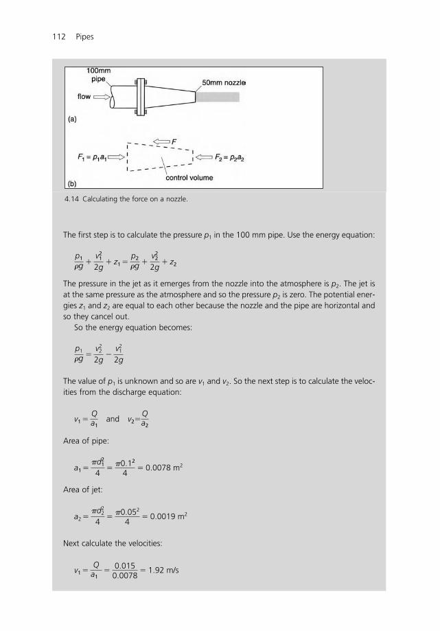
112 Pipes
The first step is to calculate the pressure p1 in the 100 mm pipe. Use the energy equation:
The pressure in the jet as it emerges from the nozzle into the atmosphere is p2. The jet isat the same pressure as the atmosphere and so the pressure p2 is zero. The potential ener-gies z1 and z2 are equal to each other because the nozzle and the pipe are horizontal andso they cancel out.
So the energy equation becomes:
The value of p1 is unknown and so are v1 and v2. So the next step is to calculate the veloc-ities from the discharge equation:
and
Area of pipe:
Area of jet:
Next calculate the velocities:
v1
�
Qa1
�
0.0150.0078
� 1.92 m/s
a2
�
�d22
4 �
�0.052
4 � 0.0019 m2
a1
�
�d12
4 �
�0.12
4 � 0.0078 m2
v2�Qa2
v1
�
Qa1
p1
�g �
v22
2g �
v21
2g
p1
�g �
v21
2g � z1
�
p2
�g �
v22
2g � z2
4.14 Calculating the force on a nozzle.
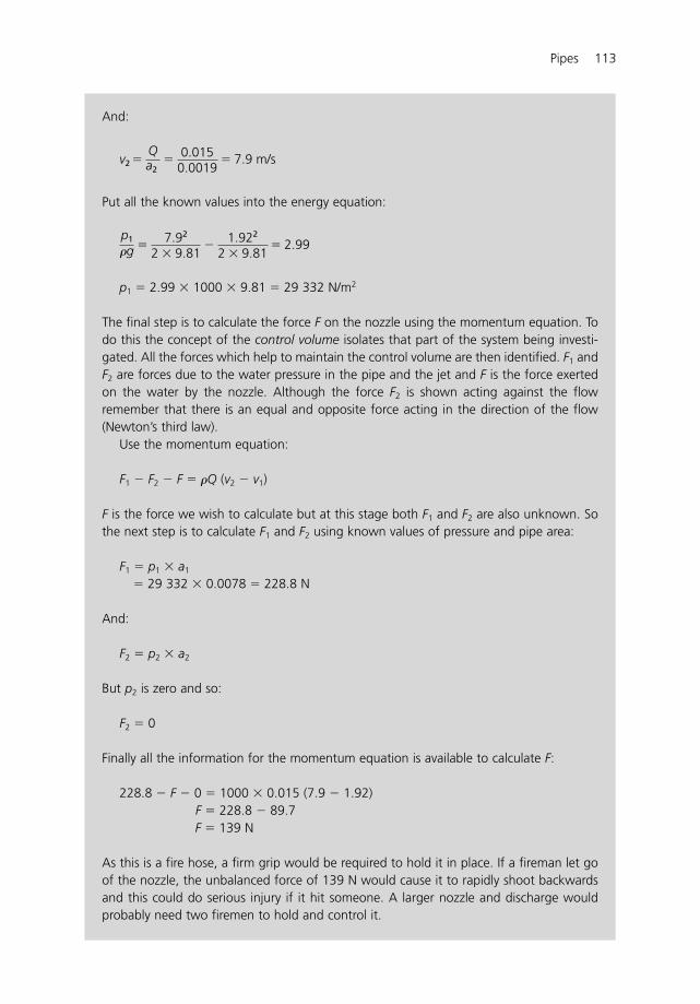
Pipes 113
And:
Put all the known values into the energy equation:
p1 � 2.99 � 1000 � 9.81 � 29 332 N/m2
The final step is to calculate the force F on the nozzle using the momentum equation. Todo this the concept of the control volume isolates that part of the system being investi-gated. All the forces which help to maintain the control volume are then identified. F1 andF2 are forces due to the water pressure in the pipe and the jet and F is the force exertedon the water by the nozzle. Although the force F2 is shown acting against the flowremember that there is an equal and opposite force acting in the direction of the flow(Newton’s third law).
Use the momentum equation:
F1 � F2 � F � �Q (v2 � v1)
F is the force we wish to calculate but at this stage both F1 and F2 are also unknown. Sothe next step is to calculate F1 and F2 using known values of pressure and pipe area:
F1 � p1 � a1
� 29 332 � 0.0078 � 228.8 N
And:
F2 � p2 � a2
But p2 is zero and so:
F2 � 0
Finally all the information for the momentum equation is available to calculate F:
228.8 � F � 0 � 1000 � 0.015 (7.9 � 1.92)F � 228.8 � 89.7F � 139 N
As this is a fire hose, a firm grip would be required to hold it in place. If a fireman let goof the nozzle, the unbalanced force of 139 N would cause it to rapidly shoot backwardsand this could do serious injury if it hit someone. A larger nozzle and discharge wouldprobably need two firemen to hold and control it.
p1
�g �
7.92
2 � 9.81 �
1.922
2 � 9.81 � 2.99
v2
�
Qa2
�
0.0150.0019
� 7.9 m/s
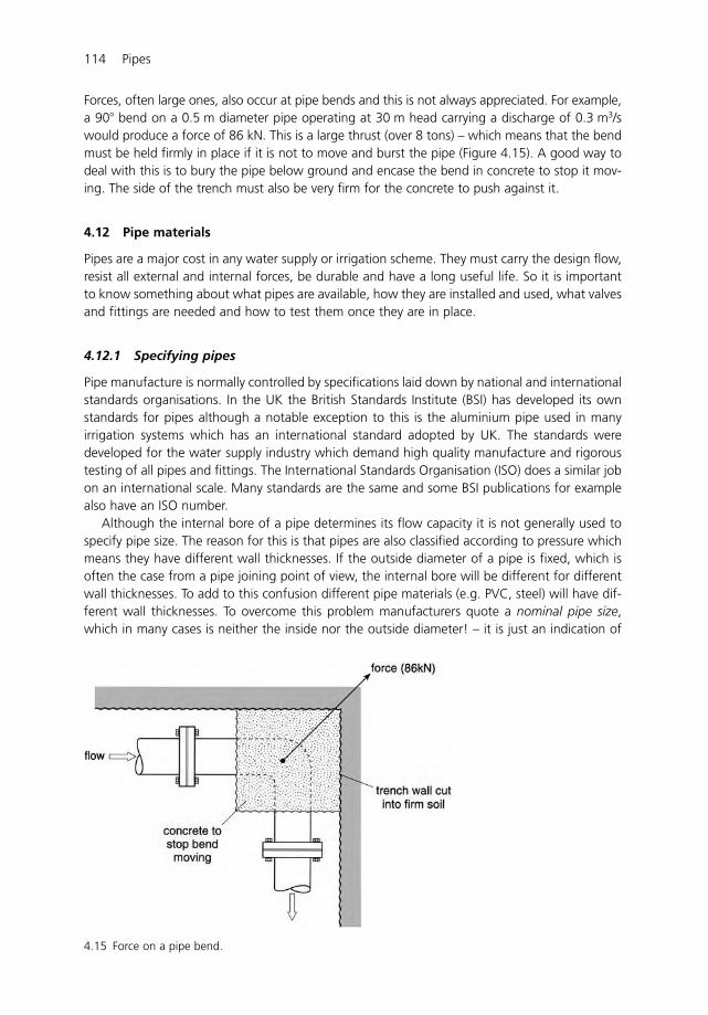
Forces, often large ones, also occur at pipe bends and this is not always appreciated. For example,a 90� bend on a 0.5 m diameter pipe operating at 30 m head carrying a discharge of 0.3 m3/swould produce a force of 86 kN. This is a large thrust (over 8 tons) – which means that the bendmust be held firmly in place if it is not to move and burst the pipe (Figure 4.15). A good way todeal with this is to bury the pipe below ground and encase the bend in concrete to stop it mov-ing. The side of the trench must also be very firm for the concrete to push against it.
4.12 Pipe materials
Pipes are a major cost in any water supply or irrigation scheme. They must carry the design flow,resist all external and internal forces, be durable and have a long useful life. So it is importantto know something about what pipes are available, how they are installed and used, what valvesand fittings are needed and how to test them once they are in place.
4.12.1 Specifying pipes
Pipe manufacture is normally controlled by specifications laid down by national and internationalstandards organisations. In the UK the British Standards Institute (BSI) has developed its ownstandards for pipes although a notable exception to this is the aluminium pipe used in manyirrigation systems which has an international standard adopted by UK. The standards weredeveloped for the water supply industry which demand high quality manufacture and rigoroustesting of all pipes and fittings. The International Standards Organisation (ISO) does a similar jobon an international scale. Many standards are the same and some BSI publications for examplealso have an ISO number.
Although the internal bore of a pipe determines its flow capacity it is not generally used tospecify pipe size. The reason for this is that pipes are also classified according to pressure whichmeans they have different wall thicknesses. If the outside diameter of a pipe is fixed, which isoften the case from a pipe joining point of view, the internal bore will be different for differentwall thicknesses. To add to this confusion different pipe materials (e.g. PVC, steel) will have dif-ferent wall thicknesses. To overcome this problem manufacturers quote a nominal pipe size,which in many cases is neither the inside nor the outside diameter! – it is just an indication of
114 Pipes
4.15 Force on a pipe bend.
Pipes 115
the pipe diameter for selection purposes. It is also normal to specify the safe working pressureat which the pipes can be used.
4.12.2 Materials
Pipes are made from a wide variety of materials but the most common in water systems are steel,asbestos cement and various plastics. Steel pipes tend to be used only where very high pressuresare encountered or in conjunction with other pipe materials where extra strength is needed, suchas under roads or across ditches. Larger pipes are made from steel plate bent or rolled to shapeand butt welded. But small sizes up to 450 mm are made from hot steel ingots which are piercedand rolled into a cylinder of the right dimensions. Corrosion is a problem with steel and so pipesare wrapped with bituminous materials or galvanising. Buried pipes often use cathodic protec-tion. Corrosion is an electrolytic process set up between the pipe and the surrounding soil. It is abit like a battery with the steel pipe acting as an anode which gradually corrodes. The process isreversed by making the pipe a cathode either by connecting it to an expendable anodic materialsuch as magnesium or by passing a small electric current through the pipe material.
Asbestos cement pipes are still used in many countries for underground mains and are madefrom cement and asbestos fibre mixed in a slurry and deposited layer upon layer on a rollingmandrel. The pipe is then dipped in cold bitumen for protection and the end turned down to aspecific diameter for jointing purposes. Unlike steel, asbestos cement does not corrode easily butit is easily damaged by shock loads and must be handled with care. Sometimes damage is notalways apparent as in the case of hairline fractures. These only show up when the pipe is beingsite tested and leaks occur. Joints are made using an asbestos cement collar and rubber sealingrings similar to those used for PVC pipes. Bends and fittings cannot be made from asbestoscement and so ductile iron is used. An important criterion is that the outside diameter of theductile steel must be the same as the asbestos cement so they can be effectively joined together.
Several plastic materials are in common use for making pipes. Unplasticised polyvinyl chlo-ride (UPVC) is a rigid material and an alternative to asbestos cement, which is falling out offavour because of the health risks associated with asbestos fibres. Pipes come in various pres-sure classes and are colour coded for easy recognition. They are virtually corrosion free, light inweight, flexible and easily jointed by a spigot and socket system using either a chemical solventor rubber ring to create a seal. But laying PVC pipes needs care. They are easily damaged bysharp stones in the soil and distorted by poor compaction of material on the bottom and sidesof trenches. Hydraulically PVC has a very low friction characteristic, but it can be easily damagedinternally by sand and silt particles in the flowing water.
In contrast polythene pipe is very flexible and comes in high density and low density forms.Low density pipe is cheaper than high density and is used extensively for trickle and some sprin-kler irrigation systems where pipes are laid out on the ground. The pipe wall is thin and so it iseasily damaged by sharp tools or animals biting through it. However, it will stand up to quitehigh water pressures. High density pipes are much stronger, but more expensive and are usedextensively for domestic water supply systems.
4.13 Pipe fittings
Pipelines require a wide range of valves and special fittings to make sure the discharge is alwaysunder control. Some of the more important are sluice valves, air valves, non-return valves andcontrol valves (Figure 4.16).
Sluice valves are essentially on-off valves. They can be used to control pressure and dischargebut they are rather crude and need constant attention. It is only the last 10% of the gate opening
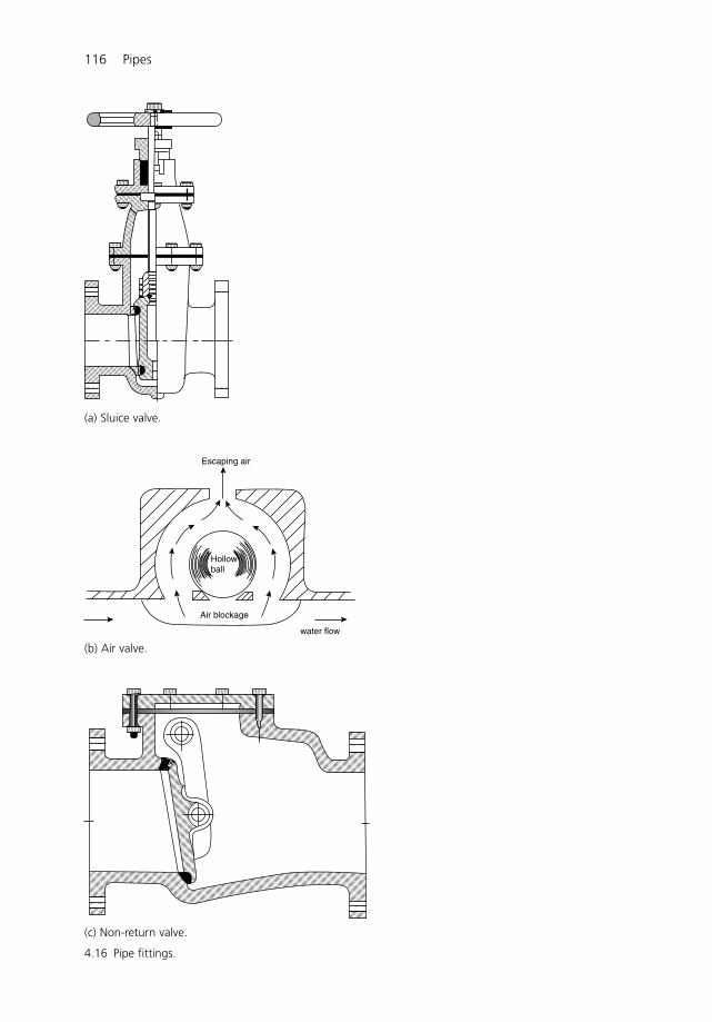
116 Pipes
(a) Sluice valve.
Air blockage
Hollowball
Escaping air
water flow
(b) Air valve.
(c) Non-return valve.
4.16 Pipe fittings.
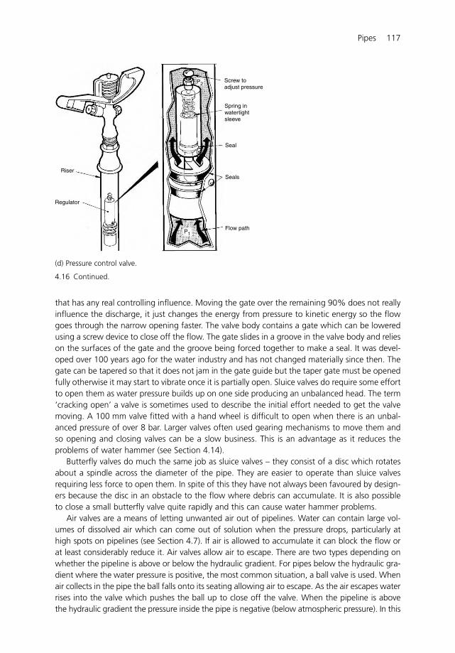
Pipes 117
that has any real controlling influence. Moving the gate over the remaining 90% does not reallyinfluence the discharge, it just changes the energy from pressure to kinetic energy so the flowgoes through the narrow opening faster. The valve body contains a gate which can be loweredusing a screw device to close off the flow. The gate slides in a groove in the valve body and relieson the surfaces of the gate and the groove being forced together to make a seal. It was devel-oped over 100 years ago for the water industry and has not changed materially since then. Thegate can be tapered so that it does not jam in the gate guide but the taper gate must be openedfully otherwise it may start to vibrate once it is partially open. Sluice valves do require some effortto open them as water pressure builds up on one side producing an unbalanced head. The term‘cracking open’ a valve is sometimes used to describe the initial effort needed to get the valvemoving. A 100 mm valve fitted with a hand wheel is difficult to open when there is an unbal-anced pressure of over 8 bar. Larger valves often used gearing mechanisms to move them andso opening and closing valves can be a slow business. This is an advantage as it reduces theproblems of water hammer (see Section 4.14).
Butterfly valves do much the same job as sluice valves – they consist of a disc which rotatesabout a spindle across the diameter of the pipe. They are easier to operate than sluice valvesrequiring less force to open them. In spite of this they have not always been favoured by design-ers because the disc in an obstacle to the flow where debris can accumulate. It is also possibleto close a small butterfly valve quite rapidly and this can cause water hammer problems.
Air valves are a means of letting unwanted air out of pipelines. Water can contain large vol-umes of dissolved air which can come out of solution when the pressure drops, particularly athigh spots on pipelines (see Section 4.7). If air is allowed to accumulate it can block the flow orat least considerably reduce it. Air valves allow air to escape. There are two types depending onwhether the pipeline is above or below the hydraulic gradient. For pipes below the hydraulic gra-dient where the water pressure is positive, the most common situation, a ball valve is used. Whenair collects in the pipe the ball falls onto its seating allowing air to escape. As the air escapes waterrises into the valve which pushes the ball up to close off the valve. When the pipeline is abovethe hydraulic gradient the pressure inside the pipe is negative (below atmospheric pressure). In this
Screw toadjust pressure
Spring inwatertightsleeve
Riser
Regulator
Seal
Seals
Flow pathP1
P2
(d) Pressure control valve.
4.16 Continued.
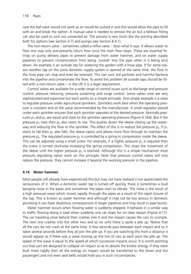
case the ball valve would not work as air would be sucked in and this would allow the pipe to fillwith air and break the siphon. A manual valve is needed to remove the air but a bellows fittingcan also be used to suck out unwanted air. This process is very much like the priming describedboth for siphons (see Section 4.7) and pumps (see Section 8.4.1).
The non-return valve – sometimes called a reflux valve – does what it says. It allows water toflow one way only and prevents return flow once the main flow stops. These are essential fit-tings on pump delivery pipes to prevent damage from water hammer, and on water supplypipelines to prevent contamination from being ‘sucked’ into the pipe when it is being shutdown. An example is an outside tap for watering the garden with a hose pipe. If for some rea-son another tap on the same domestic supply system is opened at the same time, the flow inthe hose pipe can stop and even be reversed. This can suck soil particles and harmful bacteriainto the pipeline and contaminate the flow. To avoid this problem all outside taps should be fit-ted with a non-return valve – in the UK it is a legal requirement.
Control valves are available for a wide range of control issues such as discharge and pressurecontrol, pressure reducing, pressure sustaining and surge control. Some valves now are verysophisticated and expensive but each works on a simple principle. One simple example is a valveto regulate pressure under agricultural sprinklers. Sprinklers work best when the operating pres-sure is constant and at the value recommended by the manufacturer. A small regulator placedunder each sprinkler ensures that each sprinkler operates at the desired pressure. Normally pres-sures p1 and p2 are equal and close to the sprinkler operating pressure (Figure 4.16d). But if thepressure p1 rises then p2 also starts to rise. This pushes down the sleeve closing up the water-way and reducing the flow to the sprinkler. The effect of this is to reduce the pressure p2. If p1
starts to fall then p2 also falls, the sleeve opens and allows more flow through to maintain thepressure p2. The regulated pressure p2 is controlled by a spring in compression inside the sleeve.This can be adjusted using a small screw. For example, if a higher pressure p2 is required thenthe screw is turned clockwise increasing the spring compression. This stops the movement ofthe sleeve until the higher pressure p2 is reached. Although this is a simple mechanism mostpressure regulating valves work on this principle. Note that pressure control valves will onlyreduce the pressure, they cannot increase it beyond the working pressure in the pipeline.
4.14 Water hammer
Most people will already have experienced this but may not have realised it nor appreciated theseriousness of it. When a domestic water tap is turned off quickly, there is sometimes a loudbanging noise in the pipes and sometimes the pipes start to vibrate. The noise is the result ofa high pressure wave which moves rapidly through the pipes as a result of the rapid closure ofthe tap. This is known as water hammer and although it may not be too serious in domesticplumbing it can have disastrous consequences in larger pipelines and may result in pipe bursts.
Water hammer occurs when flowing water is suddenly stopped. It behaves in a similar wayto traffic flowing along a road when suddenly one car stops for no clear reason (Figure 4.17).The car travelling close behind then crashes into it and the impact causes the cars to crumple.The next one crashes into the other two and so on until there is quite a pile up. Notice thatall the cars do not crash at the same time. A few seconds pass between each impact and so ittakes several seconds before they all join the pile up. If you are watching this from a distance itwould appear as if there was a wave moving up the line of cars as each joins the pile up. Thespeed of the wave is equal to the speed at which successive impacts occur. It is worth pointingout that cars are designed to collapse on impact so as to absorb the kinetic energy. If they werebuilt more rigidly then all the energy on impact would be transferred to the driver and thepassengers and not even seat belts would hold you in such circumstances.
118 Pipes
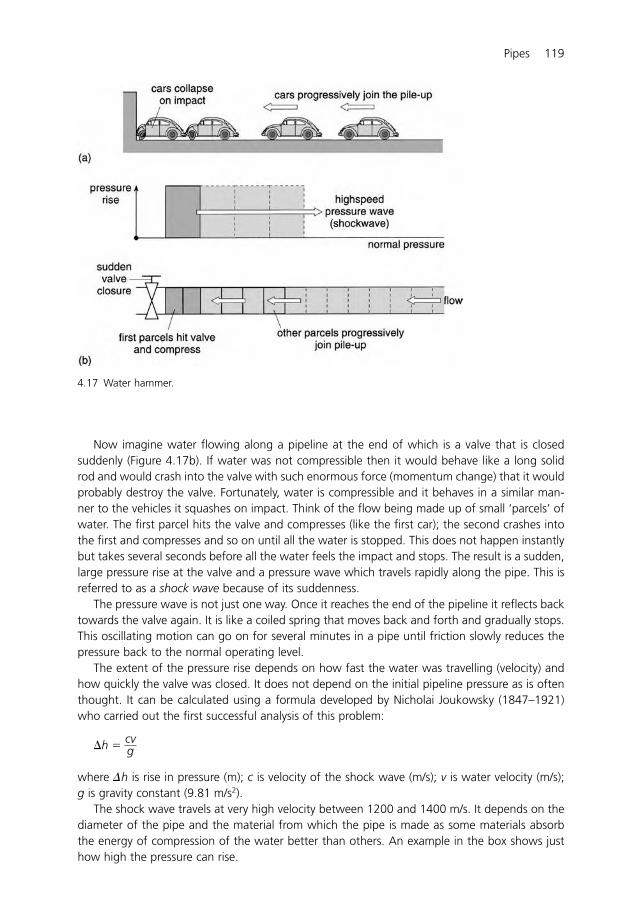
Pipes 119
Now imagine water flowing along a pipeline at the end of which is a valve that is closedsuddenly (Figure 4.17b). If water was not compressible then it would behave like a long solidrod and would crash into the valve with such enormous force (momentum change) that it wouldprobably destroy the valve. Fortunately, water is compressible and it behaves in a similar man-ner to the vehicles it squashes on impact. Think of the flow being made up of small ‘parcels’ ofwater. The first parcel hits the valve and compresses (like the first car); the second crashes intothe first and compresses and so on until all the water is stopped. This does not happen instantlybut takes several seconds before all the water feels the impact and stops. The result is a sudden,large pressure rise at the valve and a pressure wave which travels rapidly along the pipe. This isreferred to as a shock wave because of its suddenness.
The pressure wave is not just one way. Once it reaches the end of the pipeline it reflects backtowards the valve again. It is like a coiled spring that moves back and forth and gradually stops.This oscillating motion can go on for several minutes in a pipe until friction slowly reduces thepressure back to the normal operating level.
The extent of the pressure rise depends on how fast the water was travelling (velocity) andhow quickly the valve was closed. It does not depend on the initial pipeline pressure as is oftenthought. It can be calculated using a formula developed by Nicholai Joukowsky (1847–1921)who carried out the first successful analysis of this problem:
where �h is rise in pressure (m); c is velocity of the shock wave (m/s); v is water velocity (m/s);g is gravity constant (9.81 m/s2).
The shock wave travels at very high velocity between 1200 and 1400 m/s. It depends on thediameter of the pipe and the material from which the pipe is made as some materials absorbthe energy of compression of the water better than others. An example in the box shows justhow high the pressure can rise.
h � cvg
4.17 Water hammer.

The example of course, is an extreme one as it is difficult to close a valve instantaneously. Itis also wrong to assume that the pipe is rigid. All materials stretch when they are under pressureand so the pipe itself will absorb some of the pressure energy by expanding. All these factorshelp to reduce the pressure rise but they do not stop it. Even if the pressure rise is only half theabove value (say 6 bar) it is still a high pressure to suddenly cope with and this too is enough toburst the pipe. When pipes burst they usually open up along their length rather than aroundtheir circumference. They burst open rather like unzipping a coat.
Reducing water hammer problems is similar to reducing car crash problems. When cars aremoving slowly then the force of impact is not as great. Also when the first car slows down grad-ually then the others are unlikely to crash into it. Similarly, when water is moving more slowlythe pressure rises when a valve closes is reduced (see Joukowsky equation). This is one of thereasons why most pipeline designers restrict velocities to below 1.6 m/s so as to reduce waterhammer problems. Also, when valves are closed slowly, water slows down gradually and thereis little or no pressure rise along the pipe.
In summary to reduce the effects of water hammer:
� Make sure water velocities are low (below 1.6 m/s).� Close control valves slowly.
In some cases it is not always possible to avoid the sudden closure of a pipeline. For exam-ple, if a heavy vehicle drives over pipes laid out on the ground, such as might occur with fire
120 Pipes
EXAMPLE: CALCULATING PRESSURE RISE IN A PIPELINEDUE TO WATER HAMMER
Using the Joukowsky equation determine the pressure rise in a pipeline when it is suddenlyclosed. The normal pipeline velocity is 1.0 m/s and the shock wave velocity is 1200 m/s.
If the pipeline is 10 km long determine how long it takes for the pressure wave totravel the length of the pipeline.
Using the Joukowsky equation:
pressure rise � 122 m
So the pressure rise would be 122 m head of water or 12.2 bar. This is on top of thenormal operating pressure of the pipe and could well cause the pipe to burst.
Calculate the time it takes the wave to travel the length of the pipe:
It takes only 8 s for the shock wave to travel the 10 km length of the pipe and 16 s forthis to return to the valve.
time �
distancevelocity
�
10 0001200
� 8 s
� 1200�1.09.81
h � cvg
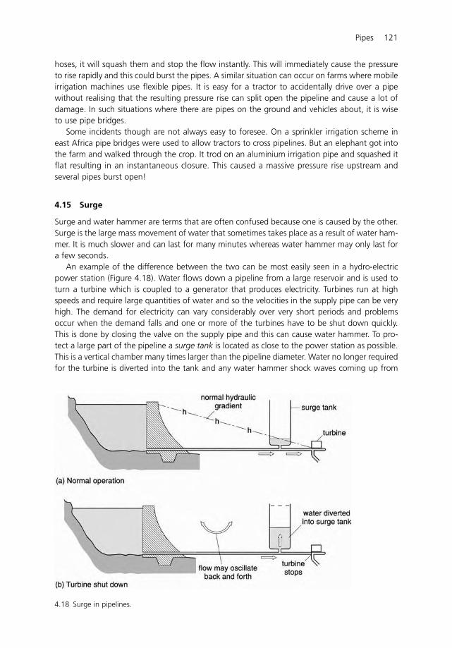
Pipes 121
hoses, it will squash them and stop the flow instantly. This will immediately cause the pressureto rise rapidly and this could burst the pipes. A similar situation can occur on farms where mobileirrigation machines use flexible pipes. It is easy for a tractor to accidentally drive over a pipewithout realising that the resulting pressure rise can split open the pipeline and cause a lot ofdamage. In such situations where there are pipes on the ground and vehicles about, it is wiseto use pipe bridges.
Some incidents though are not always easy to foresee. On a sprinkler irrigation scheme ineast Africa pipe bridges were used to allow tractors to cross pipelines. But an elephant got intothe farm and walked through the crop. It trod on an aluminium irrigation pipe and squashed itflat resulting in an instantaneous closure. This caused a massive pressure rise upstream andseveral pipes burst open!
4.15 Surge
Surge and water hammer are terms that are often confused because one is caused by the other.Surge is the large mass movement of water that sometimes takes place as a result of water ham-mer. It is much slower and can last for many minutes whereas water hammer may only last fora few seconds.
An example of the difference between the two can be most easily seen in a hydro-electricpower station (Figure 4.18). Water flows down a pipeline from a large reservoir and is used toturn a turbine which is coupled to a generator that produces electricity. Turbines run at highspeeds and require large quantities of water and so the velocities in the supply pipe can be veryhigh. The demand for electricity can vary considerably over very short periods and problemsoccur when the demand falls and one or more of the turbines have to be shut down quickly.This is done by closing the valve on the supply pipe and this can cause water hammer. To pro-tect a large part of the pipeline a surge tank is located as close to the power station as possible.This is a vertical chamber many times larger than the pipeline diameter. Water no longer requiredfor the turbine is diverted into the tank and any water hammer shock waves coming up from
4.18 Surge in pipelines.
the valve closure are absorbed by the tank. Thus water hammer is confined to the pipelinebetween the turbine and the tank and so only this length of pipe needs to be constructed towithstand the high water hammer pressures. Gradually the tank fills with water and the flowfrom the reservoir slows down and eventually stops. Usually, the rushing water can cause thetank to overfill. In such cases water may flow back and forth between the tank and the reser-voir for several hours. This slow but large movement of water is called surge and although it isthe result of water hammer it is quite different in character.
Surge can also cause problems in pumping mains and these are discussed more fully inSection 8.14.
4.16 Some examples to test your understanding
1 A 150 mm pipeline is 360 m long and has a friction factor � � 0.02. Calculate the headloss in the pipeline using the Darcy–Weisbach formula when the discharge is 0.05 m3/s.Calculate the hydraulic gradient in m/100 m of pipeline (19.46 m; 5.4 m/100 m).
2 A pipeline 2.5 km long and 150 mm diameter supplies water from a reservoir to a smalltown storage tank. Calculate the discharge when the pipe outlet is freely discharging intothe tank and the difference in level between the reservoir and the outlet is 15 m. Assume� � 0.04 (0.012 m3/s).
3 Water from a large reservoir flows through a pipeline, 1.8 km long and discharges into serv-ice tank. The first 600 m of pipe is 300 mm in diameter and the remainder is 150 mm indiameter. Calculate the discharge when the difference in water level between the tworeservoirs is 25 m and � � 0.04 for both pipes (0.02 m3/s).
4 A venturi meter is fitted to a pipeline to measure discharge. The pipe diameter is 300 mmand the venturi throat diameter is 75 mm. Calculate the discharge in m3/s when the differ-ence in pressure between the pipe and the venturi throat is 400 mm of water. Assume thecoefficient of discharge is 0.97 (0.07 m3/s).
5 A pipeline is reduced in diameter from 500 mm to 300 mm using a concentric reducer pipe.Calculate the force on the reducer when the discharge is 0.35 m3/s and the pressure in the500 mm pipe is 300 kN/m2 (37.4 kN).
6 A 500 mm diameter pipeline is fitted with a 90� bend. Calculate the resultant force on thebend if the normal operating pressure is 50 m head of water and the discharge is 0.3 m3/s.Calculate the resultant force when there is no flow in the pipe but the system is still underpressure (138 kN; 137 kN).
7 Calculate the pressure rise in a 0.5 m diameter pipeline carrying a discharge of 0.3 m3/swhen a sluice valve is closed suddenly (187 m).
122 Pipes
5 Channels
5.1 Introduction
Natural rivers and man-made canals are open channels. They have many advantages over pipesand have been used for many centuries for water supply, for transport and for agriculture. TheRomans made extensive use of channels and built aqueducts for their sophisticated water supplyschemes. Barge canals are still an important means of transporting heavy bulk materials inEurope and irrigation canals bring life and prosperity to the arid lands of North Africa, MiddleEast, India and Australia as they have done for thousands of years.
5.2 Pipes or channels?
The choice between pipes and open channels is most likely to depend on which provides thecheapest solution both in terms of capital expenditure and the recurrent costs of operation andmaintenance. However, there are advantages and disadvantages with each which may influenceor restrict the final choice.
Channels, for example, are very convenient and economical for conveying large quantities ofwater over relatively flat land such as in large irrigation systems on river flood plains. It is hardto imagine some of the large irrigation canals in India and Pakistan being put into pipes,although 5 m diameter pipes are used in Libya to transport water across the desert to coastalcities and irrigation schemes. In hilly areas the cost of open channels can rise significantlybecause the alignment must follow the land contours to create a gentle downward slope for theflow. A more direct route would be too steep causing erosion and serious damage to channels.Pipes would be more suitable in such conditions. They can be used in any kind of terrain andcan take a more direct route. Water velocities too can be much higher in pipes because there isno risk of erosion.
Although there are obvious physical differences between channels and pipes, there are sev-eral important hydraulic differences between them:
� Open channels have a free or open water surface whereas pipes are enclosed and alwaysflow full.
� Water can only flow downhill in channels but in pipes it can flow both uphill and downhill.Flow in pipes depends on a pressure difference between the inlet and outlet. As long as thepressure is higher at the inlet than at the outlet then water will flow even though the
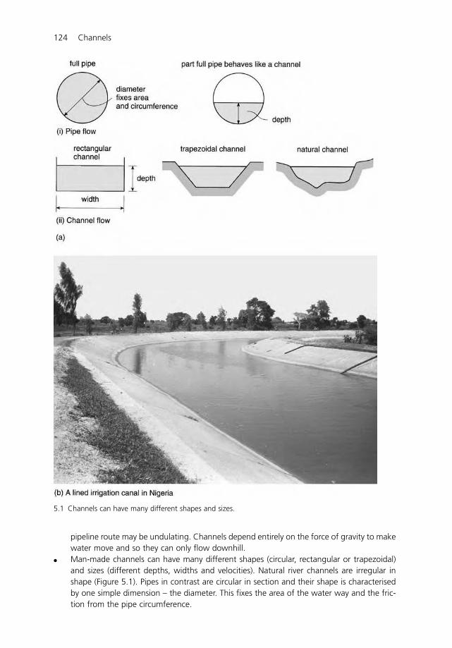
124 Channels
pipeline route may be undulating. Channels depend entirely on the force of gravity to makewater move and so they can only flow downhill.
� Man-made channels can have many different shapes (circular, rectangular or trapezoidal)and sizes (different depths, widths and velocities). Natural river channels are irregular inshape (Figure 5.1). Pipes in contrast are circular in section and their shape is characterisedby one simple dimension – the diameter. This fixes the area of the water way and the fric-tion from the pipe circumference.
5.1 Channels can have many different shapes and sizes.
Channels 125
� Water velocities are usually lower in channels than in pipes. This is because channels areoften in natural soils which erode easily. So channels are usually much larger than pipes forthe same flow.
� Channels need much more attention than pipes. They tend to erode and weeds grow inwaterways and so regular cleaning is required. Water losses from seepage and evaporationcan also be a problem.
These differences make channels a little more complicated to deal with than pipes but mostopen channel problems can be solved using the basic tools of hydraulics; discharge and conti-nuity, energy and momentum.
The study of open channels is not just confined to channel shapes and sizes. It can alsoinclude waves; the problem of handling varying flood flows down rivers and sediment transportassociated with the scouring and silting of rivers and canals. Some of these issues are touchedon in this chapter but waves are discussed more fully in Chapter 6.
5.3 Laminar and turbulent flow
Laminar and turbulent flow both occur in channels as well as in pipes. But for all practical pur-poses, flow in rivers and canals is turbulent and, like pipes, laminar flow is unlikely to occurexcept for very special conditions. For example, laminar flow only occurs in channels when thedepth is less than 25 mm and the velocity is less than 0.025 m/s. This is not a very practical sizeand velocity and so laminar flow in channels can safely be ignored. The only time it does becomeimportant is in laboratory studies where physical hydraulic models are used to simulate large andcomplex channel flow problems. Scaling down the size to fit in the laboratory often means thatthe flow in the model becomes laminar. This change in flow regime will affect the results andcare is needed when using them to assess what will happen in practice.
5.4 Using the hydraulic tools
Continuity and energy are particularly useful tools for solving open channel flow problems.Momentum is also helpful for problems in which there are energy losses and where there areforces involved.
5.4.1 Continuity
Continuity is used for open channels in much the same way as it is used for pipes (Figure 5.2a).The discharge Q1 passing point 1 in a channel must be equal to the discharge Q2 passing point 2.
Q1 � Q2
Writing this in terms of velocity and area:
v1a1 � v2a2
The term discharge per unit width (q) is often used to describe channel flow rather than the totaldischarge (Q). This is the flow in a 1.0 m wide portion of a channel (Figure 5.2b).
To calculate the discharge per unit width (q) for a rectangular channel:Use the continuity equation Q � va
where a � bd
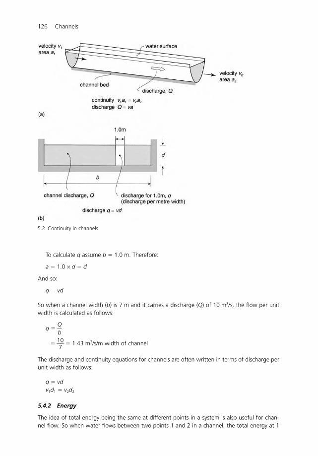
126 Channels
To calculate q assume b � 1.0 m. Therefore:
a � 1.0 × d � d
And so:
q � vd
So when a channel width (b) is 7 m and it carries a discharge (Q) of 10 m3/s, the flow per unitwidth is calculated as follows:
q �
� � 1.43 m3/s/m width of channel
The discharge and continuity equations for channels are often written in terms of discharge perunit width as follows:
q � vdv1d1 � v2d2
5.4.2 Energy
The idea of total energy being the same at different points in a system is also useful for chan-nel flow. So when water flows between two points 1 and 2 in a channel, the total energy at 1
107
Qb
5.2 Continuity in channels.
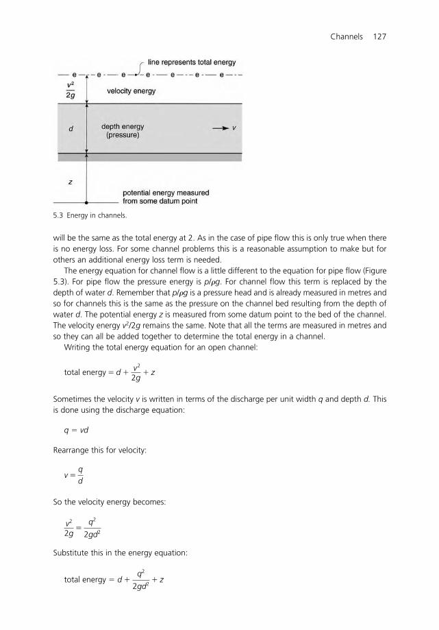
Channels 127
will be the same as the total energy at 2. As in the case of pipe flow this is only true when thereis no energy loss. For some channel problems this is a reasonable assumption to make but forothers an additional energy loss term is needed.
The energy equation for channel flow is a little different to the equation for pipe flow (Figure5.3). For pipe flow the pressure energy is p/�g. For channel flow this term is replaced by thedepth of water d. Remember that p/�g is a pressure head and is already measured in metres andso for channels this is the same as the pressure on the channel bed resulting from the depth ofwater d. The potential energy z is measured from some datum point to the bed of the channel.The velocity energy v2/2g remains the same. Note that all the terms are measured in metres andso they can all be added together to determine the total energy in a channel.
Writing the total energy equation for an open channel:
Sometimes the velocity v is written in terms of the discharge per unit width q and depth d. Thisis done using the discharge equation:
q � vd
Rearrange this for velocity:
So the velocity energy becomes:
Substitute this in the energy equation:
total energy � d �
q2
2gd2 � z
v2
2g�
q2
2gd2
v �qd
total energy � d �
v2
2g � z
5.3 Energy in channels.
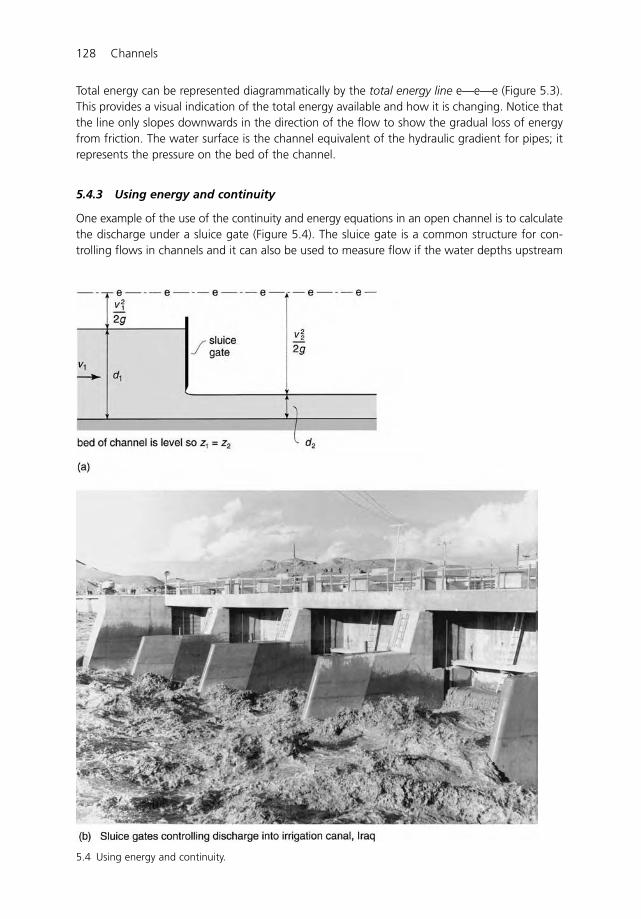
128 Channels
Total energy can be represented diagrammatically by the total energy line e—e—e (Figure 5.3).This provides a visual indication of the total energy available and how it is changing. Notice thatthe line only slopes downwards in the direction of the flow to show the gradual loss of energyfrom friction. The water surface is the channel equivalent of the hydraulic gradient for pipes; itrepresents the pressure on the bed of the channel.
5.4.3 Using energy and continuity
One example of the use of the continuity and energy equations in an open channel is to calculatethe discharge under a sluice gate (Figure 5.4). The sluice gate is a common structure for con-trolling flows in channels and it can also be used to measure flow if the water depths upstream
5.4 Using energy and continuity.
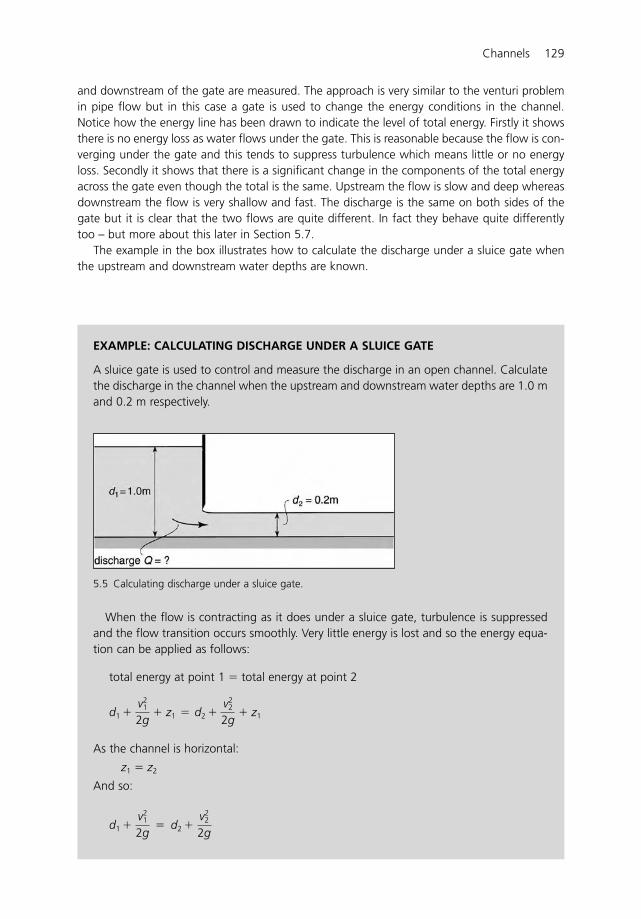
Channels 129
EXAMPLE: CALCULATING DISCHARGE UNDER A SLUICE GATE
A sluice gate is used to control and measure the discharge in an open channel. Calculatethe discharge in the channel when the upstream and downstream water depths are 1.0 mand 0.2 m respectively.
and downstream of the gate are measured. The approach is very similar to the venturi problemin pipe flow but in this case a gate is used to change the energy conditions in the channel.Notice how the energy line has been drawn to indicate the level of total energy. Firstly it showsthere is no energy loss as water flows under the gate. This is reasonable because the flow is con-verging under the gate and this tends to suppress turbulence which means little or no energyloss. Secondly it shows that there is a significant change in the components of the total energyacross the gate even though the total is the same. Upstream the flow is slow and deep whereasdownstream the flow is very shallow and fast. The discharge is the same on both sides of thegate but it is clear that the two flows are quite different. In fact they behave quite differentlytoo – but more about this later in Section 5.7.
The example in the box illustrates how to calculate the discharge under a sluice gate whenthe upstream and downstream water depths are known.
5.5 Calculating discharge under a sluice gate.
When the flow is contracting as it does under a sluice gate, turbulence is suppressedand the flow transition occurs smoothly. Very little energy is lost and so the energy equa-tion can be applied as follows:
total energy at point 1 � total energy at point 2
As the channel is horizontal:
z1 � z2
And so:
d1 � v2
1
2g � d2 �
v22
2g
d1 � v2
1
2g � z1 � d2 �
v22
2g � z1
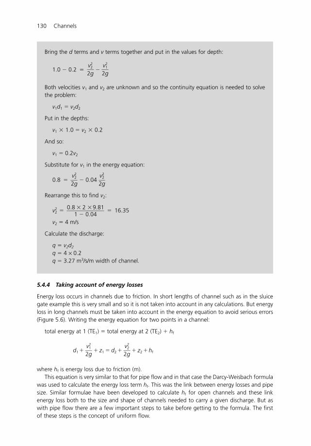
130 Channels
Bring the d terms and v terms together and put in the values for depth:
Both velocities v1 and v2 are unknown and so the continuity equation is needed to solvethe problem:
v1d1 � v2d2
Put in the depths:
v1 � 1.0 � v2 � 0.2
And so:
v1 � 0.2v2
Substitute for v1 in the energy equation:
Rearrange this to find v2:
v2 � 4 m/s
Calculate the discharge:
q � v2d2
q � 4 × 0.2q � 3.27 m3/s/m width of channel.
v22 � 0.8 � 2 �9.81
1 � 0.04 � 16.35
0.8 � v2
2
2g � 0.04
v22
2g
1.0 � 0.2 � v2
2
2g �
v21
2g
5.4.4 Taking account of energy losses
Energy loss occurs in channels due to friction. In short lengths of channel such as in the sluicegate example this is very small and so it is not taken into account in any calculations. But energyloss in long channels must be taken into account in the energy equation to avoid serious errors(Figure 5.6). Writing the energy equation for two points in a channel:
total energy at 1 (TE1) � total energy at 2 (TE2) � hf
where hf is energy loss due to friction (m).This equation is very similar to that for pipe flow and in that case the Darcy-Weisbach formula
was used to calculate the energy loss term hf. This was the link between energy losses and pipesize. Similar formulae have been developed to calculate hf for open channels and these linkenergy loss both to the size and shape of channels needed to carry a given discharge. But aswith pipe flow there are a few important steps to take before getting to the formula. The firstof these steps is the concept of uniform flow.
d1
�
v21
2g � z1 � d2
�
v22
2g � z2
�
hf

Channels 131
5.5 Uniform flow
All the energy loss formulae for open channels are based on uniform flow. This is a special conditionthat only occurs when water flows down a long, straight, gently sloping channel (Figure 5.7). Theflow is pulled down the slope by the force of gravity but there is friction from the bed and sides ofthe channel slowing it down. When the friction force is larger than the gravity force it slows downthe flow. When the friction force is smaller than the gravity force the flow moves faster down theslope. But the friction force is not constant, it depends on velocity and so as the velocity increasesso does the friction force. At some point the two forces become equal. Here the forces are inbalance and as the flow continues down the channel the depth and velocity remain constant. Thisflow condition is called uniform flow and the water depth is called the normal depth.
Unfortunately, in most channels this balance of forces rarely occurs and so the depth andvelocity are usually changing gradually even though the discharge is constant. Even in longchannels where uniform flow has a chance of occurring there is usually some variation inchannel shape or slope or a hydraulic structure which changes the depth and the velocity(Figure 5.7c). So most channels have non-uniform flow. It is also called gradually varied flowbecause the changes take place gradually along the channel.
So if non-uniform flow is the most common and uniform flow rarely occurs, why are all theformulae based on uniform flow? Why not accept that non-uniform flow is the norm anddevelop formulae for this condition? The answer is quite simple. Uniform flow is much easier todeal with from a calculation point of view and engineers are always looking for ways ofsimplifying problems but without losing accuracy. There are methods of designing channels fornon-uniform flow but they are much more cumbersome to use and usually they produce thesame shape and size of channel as uniform flow methods. So it has become accepted practice toassume that channel flow is uniform for all practical purposes. For all gently sloping channels onflood plains (i.e. 99% of all channels including rivers, canals and drainage ditches) this assumptionis a good one. Only in steep sloping channels in the mountains does it cause problems.
Remember too that great accuracy may not be necessary for designing channels anddimensions do not need to be calculated to the nearest millimetre for construction purposes.The nearest 0.05 m is accurate enough for concrete channels and probably 0.1 m for earthchannels is more than enough. From a practical construction point of view it will be difficult to
5.6 Energy losses in channels.
sloping energy line shows energy loss
datum line (horizontal)
TE1 TE2
hf
e e e e
v2
v1
21
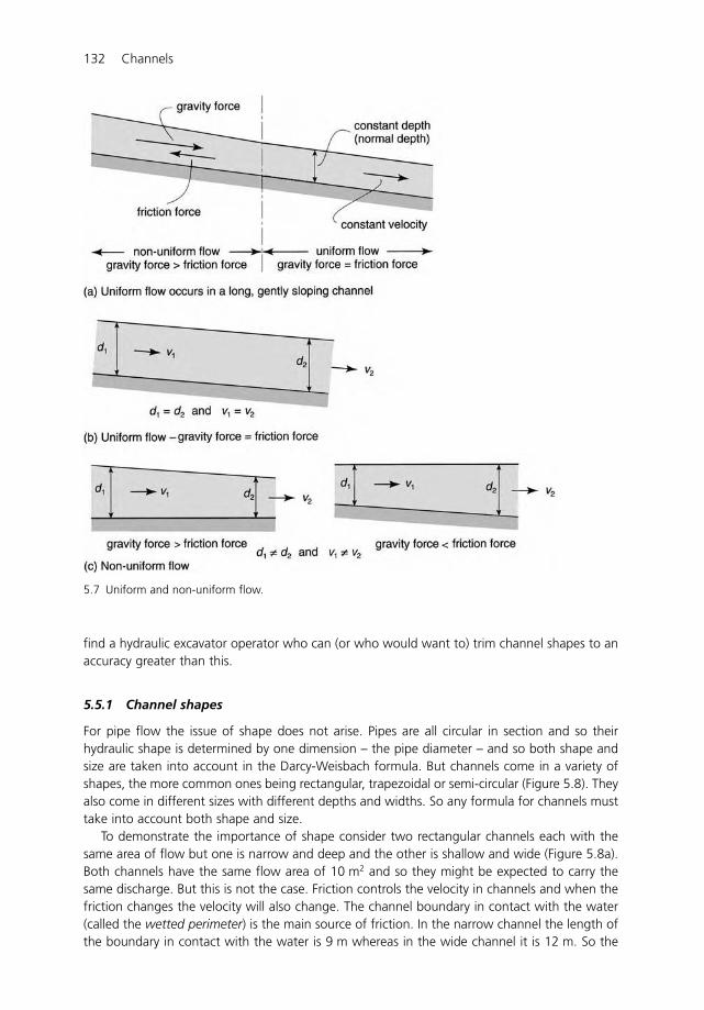
132 Channels
5.7 Uniform and non-uniform flow.
find a hydraulic excavator operator who can (or who would want to) trim channel shapes to anaccuracy greater than this.
5.5.1 Channel shapes
For pipe flow the issue of shape does not arise. Pipes are all circular in section and so theirhydraulic shape is determined by one dimension – the pipe diameter – and so both shape andsize are taken into account in the Darcy-Weisbach formula. But channels come in a variety ofshapes, the more common ones being rectangular, trapezoidal or semi-circular (Figure 5.8). Theyalso come in different sizes with different depths and widths. So any formula for channels musttake into account both shape and size.
To demonstrate the importance of shape consider two rectangular channels each with thesame area of flow but one is narrow and deep and the other is shallow and wide (Figure 5.8a).Both channels have the same flow area of 10 m2 and so they might be expected to carry thesame discharge. But this is not the case. Friction controls the velocity in channels and when thefriction changes the velocity will also change. The channel boundary in contact with the water(called the wetted perimeter) is the main source of friction. In the narrow channel the length ofthe boundary in contact with the water is 9 m whereas in the wide channel it is 12 m. So the
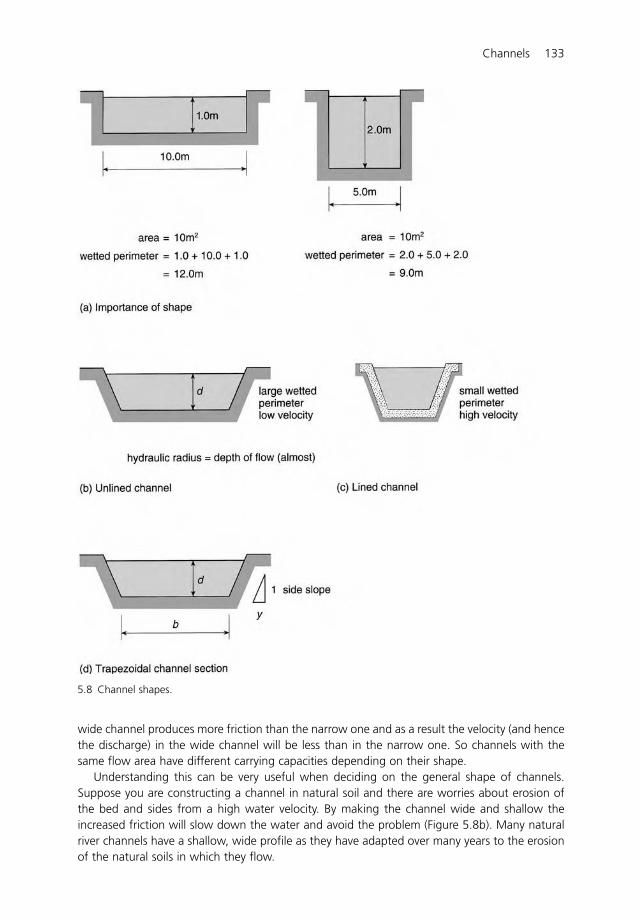
Channels 133
5.8 Channel shapes.
wide channel produces more friction than the narrow one and as a result the velocity (and hencethe discharge) in the wide channel will be less than in the narrow one. So channels with thesame flow area have different carrying capacities depending on their shape.
Understanding this can be very useful when deciding on the general shape of channels.Suppose you are constructing a channel in natural soil and there are worries about erosion ofthe bed and sides from a high water velocity. By making the channel wide and shallow theincreased friction will slow down the water and avoid the problem (Figure 5.8b). Many naturalriver channels have a shallow, wide profile as they have adapted over many years to the erosionof the natural soils in which they flow.
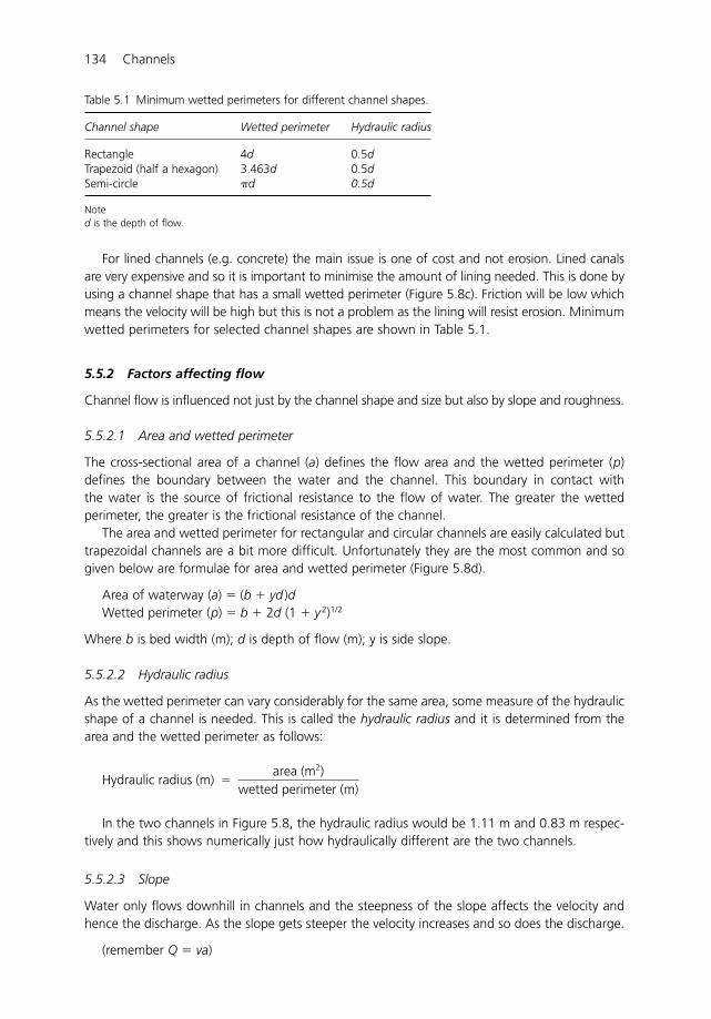
134 Channels
For lined channels (e.g. concrete) the main issue is one of cost and not erosion. Lined canalsare very expensive and so it is important to minimise the amount of lining needed. This is done byusing a channel shape that has a small wetted perimeter (Figure 5.8c). Friction will be low whichmeans the velocity will be high but this is not a problem as the lining will resist erosion. Minimumwetted perimeters for selected channel shapes are shown in Table 5.1.
5.5.2 Factors affecting flow
Channel flow is influenced not just by the channel shape and size but also by slope and roughness.
5.5.2.1 Area and wetted perimeter
The cross-sectional area of a channel (a) defines the flow area and the wetted perimeter (p)defines the boundary between the water and the channel. This boundary in contact withthe water is the source of frictional resistance to the flow of water. The greater the wettedperimeter, the greater is the frictional resistance of the channel.
The area and wetted perimeter for rectangular and circular channels are easily calculated buttrapezoidal channels are a bit more difficult. Unfortunately they are the most common and sogiven below are formulae for area and wetted perimeter (Figure 5.8d).
Area of waterway (a) � (b � yd )dWetted perimeter (p) � b � 2d (1 � y2)1/2
Where b is bed width (m); d is depth of flow (m); y is side slope.
5.5.2.2 Hydraulic radius
As the wetted perimeter can vary considerably for the same area, some measure of the hydraulicshape of a channel is needed. This is called the hydraulic radius and it is determined from thearea and the wetted perimeter as follows:
In the two channels in Figure 5.8, the hydraulic radius would be 1.11 m and 0.83 m respec-tively and this shows numerically just how hydraulically different are the two channels.
5.5.2.3 Slope
Water only flows downhill in channels and the steepness of the slope affects the velocity andhence the discharge. As the slope gets steeper the velocity increases and so does the discharge.
(remember Q � va)
Hydraulic radius (m) � area (m2)
wetted perimeter (m)
Table 5.1 Minimum wetted perimeters for different channel shapes.
Channel shape Wetted perimeter Hydraulic radius
Rectangle 4d 0.5dTrapezoid (half a hexagon) 3.463d 0.5dSemi-circle �d 0.5d
Noted is the depth of flow.
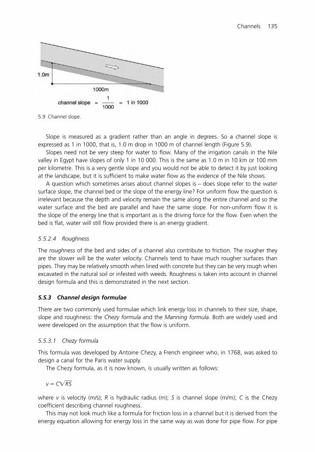
Channels 135
Slope is measured as a gradient rather than an angle in degrees. So a channel slope isexpressed as 1 in 1000, that is, 1.0 m drop in 1000 m of channel length (Figure 5.9).
Slopes need not be very steep for water to flow. Many of the irrigation canals in the Nilevalley in Egypt have slopes of only 1 in 10 000. This is the same as 1.0 m in 10 km or 100 mmper kilometre. This is a very gentle slope and you would not be able to detect it by just lookingat the landscape, but it is sufficient to make water flow as the evidence of the Nile shows.
A question which sometimes arises about channel slopes is – does slope refer to the watersurface slope, the channel bed or the slope of the energy line? For uniform flow the question isirrelevant because the depth and velocity remain the same along the entire channel and so thewater surface and the bed are parallel and have the same slope. For non-uniform flow it isthe slope of the energy line that is important as is the driving force for the flow. Even when thebed is flat, water will still flow provided there is an energy gradient.
5.5.2.4 Roughness
The roughness of the bed and sides of a channel also contribute to friction. The rougher theyare the slower will be the water velocity. Channels tend to have much rougher surfaces thanpipes. They may be relatively smooth when lined with concrete but they can be very rough whenexcavated in the natural soil or infested with weeds. Roughness is taken into account in channeldesign formula and this is demonstrated in the next section.
5.5.3 Channel design formulae
There are two commonly used formulae which link energy loss in channels to their size, shape,slope and roughness: the Chezy formula and the Manning formula. Both are widely used andwere developed on the assumption that the flow is uniform.
5.5.3.1 Chezy formula
This formula was developed by Antoine Chezy, a French engineer who, in 1768, was asked todesign a canal for the Paris water supply.
The Chezy formula, as it is now known, is usually written as follows:
where v is velocity (m/s); R is hydraulic radius (m); S is channel slope (m/m); C is the Chezycoefficient describing channel roughness.
This may not look much like a formula for friction loss in a channel but it is derived from theenergy equation allowing for energy loss in the same way as was done for pipe flow. For pipe
v � C�RS
5.9 Channel slope.
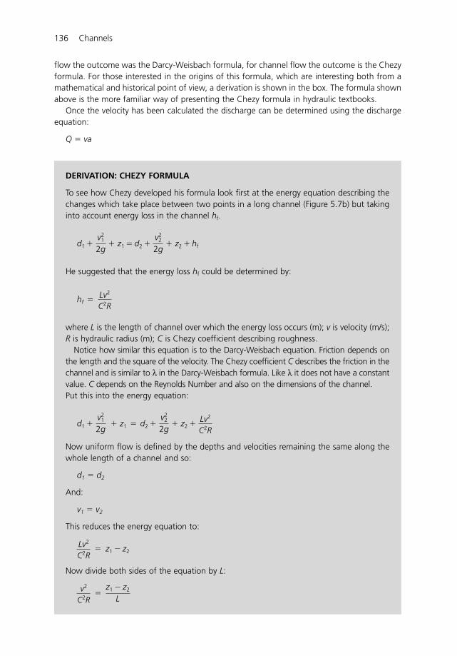
136 Channels
flow the outcome was the Darcy-Weisbach formula, for channel flow the outcome is the Chezyformula. For those interested in the origins of this formula, which are interesting both from amathematical and historical point of view, a derivation is shown in the box. The formula shownabove is the more familiar way of presenting the Chezy formula in hydraulic textbooks.
Once the velocity has been calculated the discharge can be determined using the dischargeequation:
Q � va
DERIVATION: CHEZY FORMULA
To see how Chezy developed his formula look first at the energy equation describing thechanges which take place between two points in a long channel (Figure 5.7b) but takinginto account energy loss in the channel hf.
He suggested that the energy loss hf could be determined by:
where L is the length of channel over which the energy loss occurs (m); v is velocity (m/s);R is hydraulic radius (m); C is Chezy coefficient describing roughness.
Notice how similar this equation is to the Darcy-Weisbach equation. Friction depends onthe length and the square of the velocity. The Chezy coefficient C describes the friction in thechannel and is similar to λ in the Darcy-Weisbach formula. Like λ it does not have a constantvalue. C depends on the Reynolds Number and also on the dimensions of the channel.Put this into the energy equation:
Now uniform flow is defined by the depths and velocities remaining the same along thewhole length of a channel and so:
d1 � d2
And:
v1 � v2
This reduces the energy equation to:
Now divide both sides of the equation by L:
v2
C2R �
z1 � z2
L
Lv2
C2R � z1 � z2
d1 � v2
1
2g � z1 � d2 �
v22
2g � z2 � Lv2
C2R
hf � Lv2
C2R
d1 � v2
1
2g � z1 � d2 �
v22
2g � z2 � hf

Channels 137
Table 5.2 Values of Manning's n.
Channel type Manning's n values
Concrete lined canals 0.012–0.017Rough masonry 0.017–0.030Roughly dug earth canals 0.025–0.033Smooth earth canals 0.017–0.025Natural river in gravel 0.040–0.070
But is the slope of the channel bed S. It is also the slope of the water surface.
Remember that the two are parallel for uniform flow. Hence:
And so:
Rearrange this to calculate the velocity:
This is the familiar form of the Chezy equation that is quoted in hydraulic text books.
v � C�RS
v2
C2R � S
z1�z2
L � S
z1�z2
L
5.5.3.2 Manning formula
The Manning formula is an alternative to Chezy and is one of the most commonly used formu-lae for designing channels. This was developed by Robert Manning (1816–1897) an Irish civilengineer. It is an empirical formula developed from many observations made on natural channels.
where v is velocity (m/s); R is hydraulic radius (m); S is channel bed slope (m/m); n is Manning'sroughness coefficient.
Manning's n values depend on the surface roughness of a channel. Typical values are listedin Table 5.2.
The value of Manning's n is not just determined by the material from which the channel ismade but it is also affected by vegetation growth. This can make it difficult to determine withany accuracy. The n value can also change over time as weeds grow and it can also change withchanges in flow. At low discharges weeds and grasses will be upright and so cause great rough-ness but at higher discharges they may be flattened by the flow and so the channel becomesmuch smoother. There is an excellent book, Open Channel Flow by Ven Te Chow (see refer-ences), which has a series of pictures of channels with different weed growths and suggested nvalues. These pictures can be compared with existing channels to get some indication of n. But
v � R2/3S1/2
n
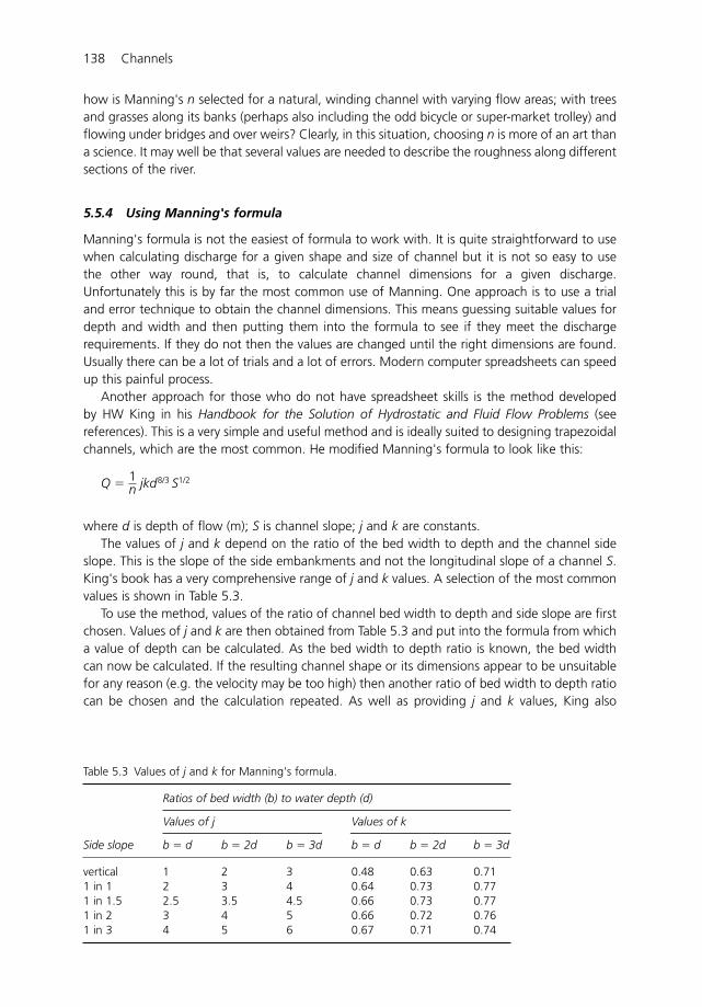
138 Channels
how is Manning's n selected for a natural, winding channel with varying flow areas; with treesand grasses along its banks (perhaps also including the odd bicycle or super-market trolley) andflowing under bridges and over weirs? Clearly, in this situation, choosing n is more of an art thana science. It may well be that several values are needed to describe the roughness along differentsections of the river.
5.5.4 Using Manning's formula
Manning's formula is not the easiest of formula to work with. It is quite straightforward to usewhen calculating discharge for a given shape and size of channel but it is not so easy to usethe other way round, that is, to calculate channel dimensions for a given discharge.Unfortunately this is by far the most common use of Manning. One approach is to use a trialand error technique to obtain the channel dimensions. This means guessing suitable values fordepth and width and then putting them into the formula to see if they meet the dischargerequirements. If they do not then the values are changed until the right dimensions are found.Usually there can be a lot of trials and a lot of errors. Modern computer spreadsheets can speedup this painful process.
Another approach for those who do not have spreadsheet skills is the method developedby HW King in his Handbook for the Solution of Hydrostatic and Fluid Flow Problems (seereferences). This is a very simple and useful method and is ideally suited to designing trapezoidalchannels, which are the most common. He modified Manning's formula to look like this:
jkd8/3 S1/2
where d is depth of flow (m); S is channel slope; j and k are constants.The values of j and k depend on the ratio of the bed width to depth and the channel side
slope. This is the slope of the side embankments and not the longitudinal slope of a channel S.King's book has a very comprehensive range of j and k values. A selection of the most commonvalues is shown in Table 5.3.
To use the method, values of the ratio of channel bed width to depth and side slope are firstchosen. Values of j and k are then obtained from Table 5.3 and put into the formula from whicha value of depth can be calculated. As the bed width to depth ratio is known, the bed widthcan now be calculated. If the resulting channel shape or its dimensions appear to be unsuitablefor any reason (e.g. the velocity may be too high) then another ratio of bed width to depth ratiocan be chosen and the calculation repeated. As well as providing j and k values, King also
Q � 1n
Table 5.3 Values of j and k for Manning's formula.
Ratios of bed width (b) to water depth (d)
Values of j Values of k
Side slope b � d b � 2d b � 3d b � d b � 2d b � 3d
vertical 1 2 3 0.48 0.63 0.711 in 1 2 3 4 0.64 0.73 0.771 in 1.5 2.5 3.5 4.5 0.66 0.73 0.771 in 2 3 4 5 0.66 0.72 0.761 in 3 4 5 6 0.67 0.71 0.74
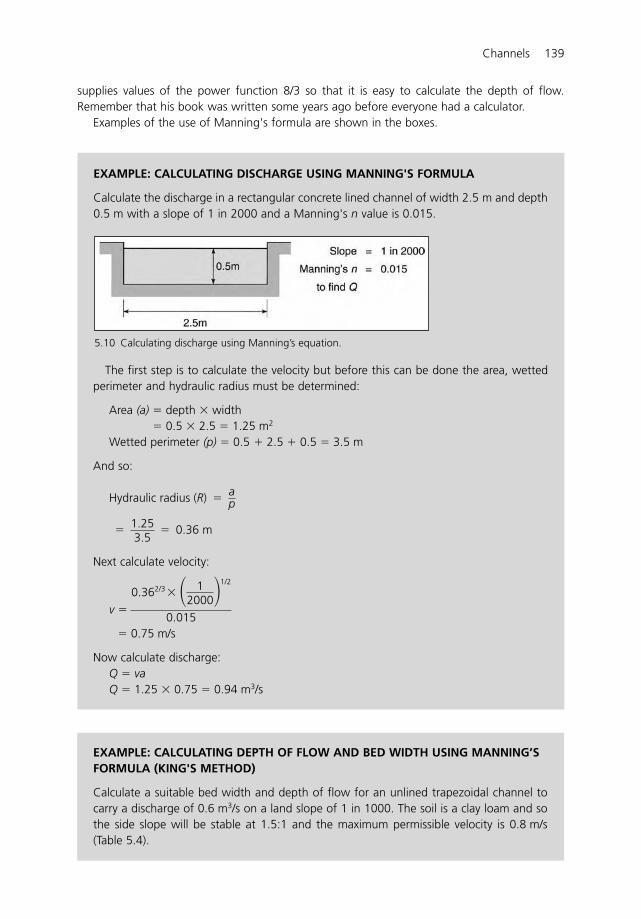
Channels 139
EXAMPLE: CALCULATING DEPTH OF FLOW AND BED WIDTH USING MANNING’SFORMULA (KING'S METHOD)
Calculate a suitable bed width and depth of flow for an unlined trapezoidal channel tocarry a discharge of 0.6 m3/s on a land slope of 1 in 1000. The soil is a clay loam and sothe side slope will be stable at 1.5:1 and the maximum permissible velocity is 0.8 m/s(Table 5.4).
EXAMPLE: CALCULATING DISCHARGE USING MANNING'S FORMULA
Calculate the discharge in a rectangular concrete lined channel of width 2.5 m and depth0.5 m with a slope of 1 in 2000 and a Manning's n value is 0.015.
5.10 Calculating discharge using Manning’s equation.
supplies values of the power function 8/3 so that it is easy to calculate the depth of flow.Remember that his book was written some years ago before everyone had a calculator.
Examples of the use of Manning's formula are shown in the boxes.
The first step is to calculate the velocity but before this can be done the area, wettedperimeter and hydraulic radius must be determined:
Area (a) � depth � width� 0.5 � 2.5 � 1.25 m2
Wetted perimeter (p) � 0.5 � 2.5 � 0.5 � 3.5 m
And so:
Next calculate velocity:
� 0.75 m/s
Now calculate discharge:Q � vaQ � 1.25 � 0.75 � 0.94 m3/s
v � 0.362/3
� � 12000�
1/2
0.015
� 1.253.5
� 0.36 m
Hydraulic radius (R) � ap
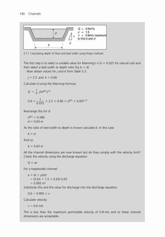
140 Channels
5.11 Calculating depth of flow and bed width using King’s method.
The first step is to select a suitable value for Manning's n (n � 0.025 for natural soil) andthen select a bed width to depth ratio (try b � d).
Now obtain values for j and k from Table 5.3.
j � 2.5 and k � 0.66
Calculate d using the Manning formula:
jkd8/3s1/2
� 2.5 � 0.66 � d8/3 � 0.0011/2
Rearrange this for d:
d8/3 � 0.286d � 0.63 m
As the ratio of bed width to depth is known calculate b. In this case:
b � d
And so:
b � 0.63 m
All the channel dimensions are now known but do they comply with the velocity limit?Check the velocity using the discharge equation:
Q � av
For a trapezoidal channel:
a � (b � yd )d� (0.63 � 1.5 � 0.63) 0.63� 0.993 m2
Substitute this and the value for discharge into the discharge equation:
0.6 � 0.993 � v
Calculate velocity:
v � 0.6 m/s
This is less than the maximum permissible velocity of 0.8 m/s and so these channeldimensions are acceptable.
0.6 � 10.025
Q � 1n
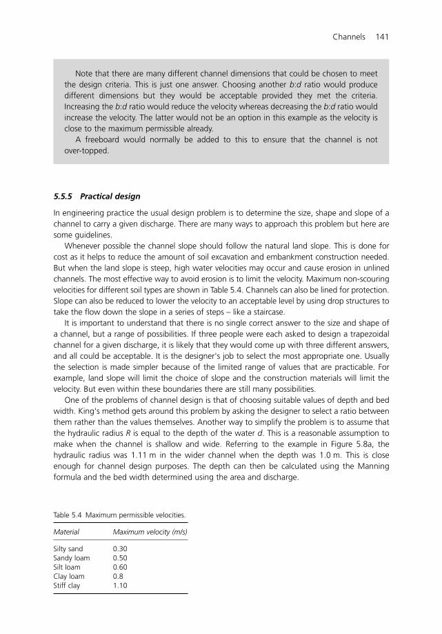
Channels 141
Table 5.4 Maximum permissible velocities.
Material Maximum velocity (m/s)
Silty sand 0.30Sandy loam 0.50Silt loam 0.60Clay loam 0.8Stiff clay 1.10
5.5.5 Practical design
In engineering practice the usual design problem is to determine the size, shape and slope of achannel to carry a given discharge. There are many ways to approach this problem but here aresome guidelines.
Whenever possible the channel slope should follow the natural land slope. This is done forcost as it helps to reduce the amount of soil excavation and embankment construction needed.But when the land slope is steep, high water velocities may occur and cause erosion in unlinedchannels. The most effective way to avoid erosion is to limit the velocity. Maximum non-scouringvelocities for different soil types are shown in Table 5.4. Channels can also be lined for protection.Slope can also be reduced to lower the velocity to an acceptable level by using drop structures totake the flow down the slope in a series of steps – like a staircase.
It is important to understand that there is no single correct answer to the size and shape ofa channel, but a range of possibilities. If three people were each asked to design a trapezoidalchannel for a given discharge, it is likely that they would come up with three different answers,and all could be acceptable. It is the designer's job to select the most appropriate one. Usuallythe selection is made simpler because of the limited range of values that are practicable. Forexample, land slope will limit the choice of slope and the construction materials will limit thevelocity. But even within these boundaries there are still many possibilities.
One of the problems of channel design is that of choosing suitable values of depth and bedwidth. King's method gets around this problem by asking the designer to select a ratio betweenthem rather than the values themselves. Another way to simplify the problem is to assume thatthe hydraulic radius R is equal to the depth of the water d. This is a reasonable assumption tomake when the channel is shallow and wide. Referring to the example in Figure 5.8a, thehydraulic radius was 1.11 m in the wider channel when the depth was 1.0 m. This is closeenough for channel design purposes. The depth can then be calculated using the Manningformula and the bed width determined using the area and discharge.
Note that there are many different channel dimensions that could be chosen to meetthe design criteria. This is just one answer. Choosing another b:d ratio would producedifferent dimensions but they would be acceptable provided they met the criteria.Increasing the b:d ratio would reduce the velocity whereas decreasing the b:d ratio wouldincrease the velocity. The latter would not be an option in this example as the velocity isclose to the maximum permissible already.
A freeboard would normally be added to this to ensure that the channel is not over-topped.
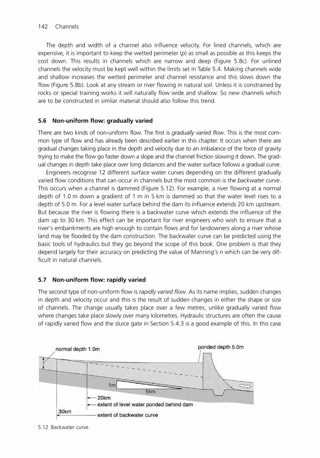
142 Channels
The depth and width of a channel also influence velocity. For lined channels, which areexpensive, it is important to keep the wetted perimeter (p) as small as possible as this keeps thecost down. This results in channels which are narrow and deep (Figure 5.8c). For unlinedchannels the velocity must be kept well within the limits set in Table 5.4. Making channels wideand shallow increases the wetted perimeter and channel resistance and this slows down theflow (Figure 5.8b). Look at any stream or river flowing in natural soil. Unless it is constrained byrocks or special training works it will naturally flow wide and shallow. So new channels whichare to be constructed in similar material should also follow this trend.
5.6 Non-uniform flow: gradually varied
There are two kinds of non-uniform flow. The first is gradually varied flow. This is the most com-mon type of flow and has already been described earlier in this chapter. It occurs when there aregradual changes taking place in the depth and velocity due to an imbalance of the force of gravitytrying to make the flow go faster down a slope and the channel friction slowing it down. The grad-ual changes in depth take place over long distances and the water surface follows a gradual curve.
Engineers recognise 12 different surface water curves depending on the different graduallyvaried flow conditions that can occur in channels but the most common is the backwater curve.This occurs when a channel is dammed (Figure 5.12). For example, a river flowing at a normaldepth of 1.0 m down a gradient of 1 m in 5 km is dammed so that the water level rises to adepth of 5.0 m. For a level water surface behind the dam its influence extends 20 km upstream.But because the river is flowing there is a backwater curve which extends the influence of thedam up to 30 km. This effect can be important for river engineers who wish to ensure that ariver's embankments are high enough to contain flows and for landowners along a river whoseland may be flooded by the dam construction. The backwater curve can be predicted using thebasic tools of hydraulics but they go beyond the scope of this book. One problem is that theydepend largely for their accuracy on predicting the value of Manning's n which can be very dif-ficult in natural channels.
5.7 Non-uniform flow: rapidly varied
The second type of non-uniform flow is rapidly varied flow. As its name implies, sudden changesin depth and velocity occur and this is the result of sudden changes in either the shape or sizeof channels. The change usually takes place over a few metres, unlike gradually varied flowwhere changes take place slowly over many kilometres. Hydraulic structures are often the causeof rapidly varied flow and the sluice gate in Section 5.4.3 is a good example of this. In this case
5.12 Backwater curve.
Channels 143
the gate changed the flow suddenly from a deep, slow flow upstream to a fast, shallow flowdownstream. Building a weir or widening (or deepening) a channel will also cause suddenchanges to occur. But unfortunately, all flows do not behave in the same way. For example, aweir in a channel will have quite a different effect on the deep, slow flow than on the shallow,fast flow. So a further classification of channel flow is needed, this time in terms of how flowbehaves when channel size or shape is changed suddenly.
The two contrasting types of flow described above are now well recognised by engineers.The more scientific name for deep, slow flow is sub-critical flow and for shallow, fast flow issuper-critical flow. This implies that there is some critical point when the flow changes from oneto the other and that this point defines the difference between the two flow types. This is indeedthe case. At the critical point the velocity becomes the critical velocity and the depth becomesthe critical depth. The critical point is important not just to classify the two flow types. It playsan important role in the measuring discharges in channels. This is discussed later in Chapter 8.
5.7.1 Flow behaviour
Just how do sub-critical and super-critical flows behave when there are sudden changes in thechannel?
5.7.1.1 Sub-critical flow
This is by far the most common flow type and is associated with all natural and gently flowingrivers and canals. The effect of a sluice gate on this kind of flow has already been described. Theeffect of a weir is very similar (Figure 5.13a). A weir is like a step up on the bed of a channel.Such a step causes the water level to drop and the velocity to increase. The step up reduces theflow area in a channel but the water does not slow down because of this. Its velocity increases(remember the way flow behaves in constrictions – Section 3.7.1). This increases the kineticenergy, but as there is no change in the total energy this is at the expense of the depth (pressure)energy. So the depth is reduced causing a drop in the water level. Weirs are a common sight onrivers and most people will have seen this sudden but smooth drop in water level over a weir. Asimilar, though not so dramatic, drop in water level occurs when water flows under a bridge. Thewater level drops because the reduced width of the river increases its velocity.
Interestingly, the converse is true. When a channel is made larger by increasing its width ordepth, the water level rises. This is not so easy to believe. But it follows from the energy equationand it actually happens in practice (Figure 5.13b). This was highlighted by a problem facing engi-neers who were troubled by flooding from a river flowing through a town and under the townbridge (Figure 5.13c). During stormy weather, the river level rises and reaches the underside ofthe bridge. The extra friction from the bridge slows the flow causing the water level upstreamof the bridge to rise even further and flood the town. The problem was how to increase the car-rying capacity of the river through the town, and particularly under the bridge, to avoid theflooding. The engineers decided that the most obvious solution was to make the channel deeper –but this made flooding worse, not better. Clearly the engineers did not understand the hydraulictools of continuity and energy. The increase in channel depth reduced the velocity and hencethe kinetic energy. As the total energy remained the same, the depth energy increased causingthe river level to rise and not fall as expected. They eventually opted for the correct solutionwhich was to reduce the flow area under the bridge by constructing a step on the bed of theriver. This increased the velocity energy and reduced the depth of flow. So even when the riverwas in flood, the flow was able to pass safely under the bridge. The local engineers did notbelieve the solution at first and insisted on building a hydraulic model in the laboratory to testit. Seeing is believing and this convinced them!
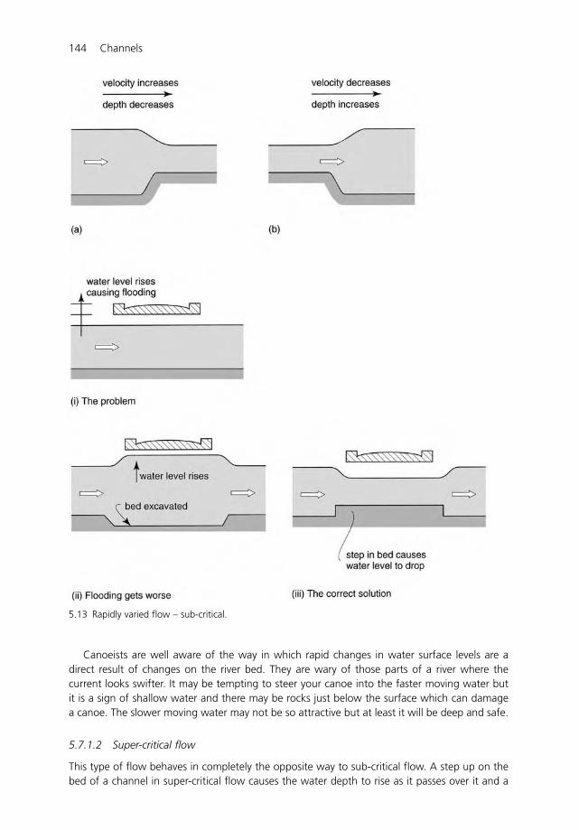
144 Channels
Canoeists are well aware of the way in which rapid changes in water surface levels are adirect result of changes on the river bed. They are wary of those parts of a river where thecurrent looks swifter. It may be tempting to steer your canoe into the faster moving water butit is a sign of shallow water and there may be rocks just below the surface which can damagea canoe. The slower moving water may not be so attractive but at least it will be deep and safe.
5.7.1.2 Super-critical flow
This type of flow behaves in completely the opposite way to sub-critical flow. A step up on thebed of a channel in super-critical flow causes the water depth to rise as it passes over it and a
5.13 Rapidly varied flow – sub-critical.
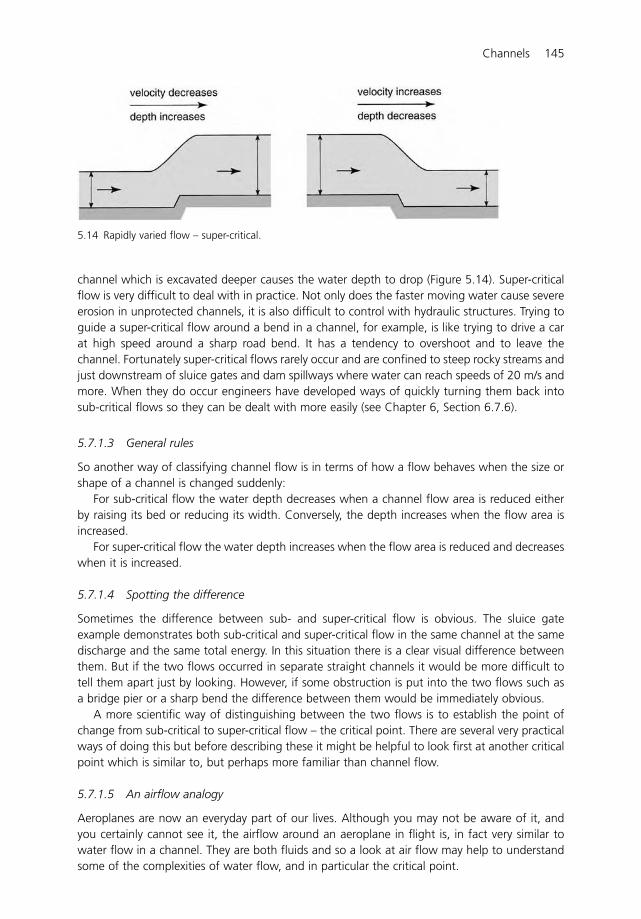
Channels 145
channel which is excavated deeper causes the water depth to drop (Figure 5.14). Super-criticalflow is very difficult to deal with in practice. Not only does the faster moving water cause severeerosion in unprotected channels, it is also difficult to control with hydraulic structures. Trying toguide a super-critical flow around a bend in a channel, for example, is like trying to drive a carat high speed around a sharp road bend. It has a tendency to overshoot and to leave thechannel. Fortunately super-critical flows rarely occur and are confined to steep rocky streams andjust downstream of sluice gates and dam spillways where water can reach speeds of 20 m/s andmore. When they do occur engineers have developed ways of quickly turning them back intosub-critical flows so they can be dealt with more easily (see Chapter 6, Section 6.7.6).
5.7.1.3 General rules
So another way of classifying channel flow is in terms of how a flow behaves when the size orshape of a channel is changed suddenly:
For sub-critical flow the water depth decreases when a channel flow area is reduced eitherby raising its bed or reducing its width. Conversely, the depth increases when the flow area isincreased.
For super-critical flow the water depth increases when the flow area is reduced and decreaseswhen it is increased.
5.7.1.4 Spotting the difference
Sometimes the difference between sub- and super-critical flow is obvious. The sluice gateexample demonstrates both sub-critical and super-critical flow in the same channel at the samedischarge and the same total energy. In this situation there is a clear visual difference betweenthem. But if the two flows occurred in separate straight channels it would be more difficult totell them apart just by looking. However, if some obstruction is put into the two flows such asa bridge pier or a sharp bend the difference between them would be immediately obvious.
A more scientific way of distinguishing between the two flows is to establish the point ofchange from sub-critical to super-critical flow – the critical point. There are several very practicalways of doing this but before describing these it might be helpful to look first at another criticalpoint which is similar to, but perhaps more familiar than channel flow.
5.7.1.5 An airflow analogy
Aeroplanes are now an everyday part of our lives. Although you may not be aware of it, andyou certainly cannot see it, the airflow around an aeroplane in flight is, in fact very similar towater flow in a channel. They are both fluids and so a look at air flow may help to understandsome of the complexities of water flow, and in particular the critical point.
5.14 Rapidly varied flow – super-critical.
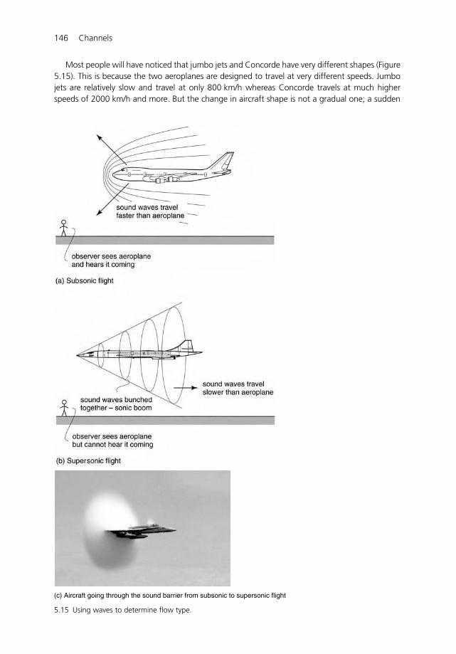
146 Channels
Most people will have noticed that jumbo jets and Concorde have very different shapes (Figure5.15). This is because the two aeroplanes are designed to travel at very different speeds. Jumbojets are relatively slow and travel at only 800 km/h whereas Concorde travels at much higherspeeds of 2000 km/h and more. But the change in aircraft shape is not a gradual one; a sudden
5.15 Using waves to determine flow type.
(c) Aircraft going through the sound barrier from subsonic to supersonic flight

Channels 147
change is needed when aeroplanes fly over 1200 km/h. This is the speed at which sound wavestravel through still air. Sound waves move through air in much the same way as waves travelacross a water surface and although they cannot be seen, they can be heard. When someonefires a gun, say 1 km away it takes 3 seconds before you hear the bang. This is the time it takesfor sound waves to travel through the air from the gun to your ear at a velocity of 1200 km/h.Notice how you see the gun flash immediately. This is because light waves travel much faster thansound waves at a velocity of 300 000 km/s. This is the reason why lightening in a storm is seenlong before the thunder is heard even when the storm is several kilometres away.
When an aeroplane is flying the noise from its engines travels outwards in all directions inthe form of sound waves. When it is travelling below the speed of sound, the sound travels fasterthan the aeroplane and so an observer hears the aeroplane coming before it reaches him (Figure5.15a). This is known as subsonic flight and aeroplanes which fly below the speed of sound havelarge rounded shapes like the jumbo jets. When an aeroplane is flying faster than the speed ofsound, the sound travels slower than the aeroplane and is left far behind. An observer will see theaeroplane approaching before hearing it (Figure 5.15b). This is known as supersonic flight and aero-planes travelling at such speeds have slim, dart-like shapes. When the observer does eventually hearit, there is usually a very loud bang. This is the result of a pressure wave, known as the sonic boom,which comes from all the sound waves being bunched up together behind the aeroplane.
So there are two types of airflow, subsonic and supersonic, and there is also a clear point atwhich the flow changes from one to the other – the speed of sound in still air.
5.7.1.6 Back to water
The purpose of this lengthy explanation about aeroplanes in flight is to demonstrate the closesimilarity between air flow and water flow. Sub-critical and super-critical flow are very similar tosubsonic and supersonic flight. The majority of aeroplanes travel at subsonic speeds and thereare very few design problems. In contrast, very few aeroplanes travel at supersonic speeds andtheir design problems are much greater and more expensive to solve. The same is true for water.Most flows are sub-critical and are easily dealt with. But in a few special cases the flow is super-critical and this is much more difficult to deal with.
The change from sub- to supersonic occurs when the aeroplane reaches the speed of soundwaves in still air. But this is where water is a little different. The change does not occur at the speedof sound in water, although sound does travel through water very effectively. It occurs when theflow reaches the same velocity as waves on the water surface. To avoid confusion between wavevelocity and water velocity, waves velocity is often referred to as wave celerity (see Section 6.2).
Waves occur on the surface of water when it is disturbed. When you throw a stone into astill pond of water, waves travel out across the surface towards the bank (Figure 5.16a).Although there seems to be a definite movement towards the bank, it is only the waves that aremoving outwards and not the water. The water only moves up and down as the waves pass. Aduck floating on the pond would only bob up and down with the wave motion and would notbe washed up on the bank! But the wave celerity is not a fixed value like the speed of sound.It depends on the depth of water and it can be calculated using the equation (see Section 6.4):
where c is wave celerity (m/s); g is gravity constant (9.81 m/s2); d is depth of water (m).So wave celerity sets the boundary between sub-critical and super-critical flow for a given
flow. When the flow velocity is less than the wave velocity the flow is sub-critical. When it isgreater, the flow is super-critical.
c � �gd
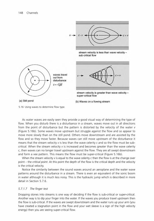
148 Channels
As water waves are easily seen they provide a good visual way of determining the type offlow. When you disturb there is a disturbance in a stream, waves move out in all directionsfrom the point of disturbance but the pattern is distorted by the velocity of the water v(Figure 5.16b). Some waves move upstream but struggle against the flow and so appear tomove more slowly than on the still pond. Others move downstream and are assisted by theflow and so they move faster. Because waves can still move upstream of the disturbance itmeans that the stream velocity v is less than the wave celerity c and so the flow must be sub-critical. When the stream velocity v is increased and becomes greater than the wave celerityc, then waves can no longer travel upstream against the flow. They are all swept downstreamand form a vee pattern. This means the flow must be super-critical (Figure 5.16b).
When the stream velocity v is equal to the wave celerity c then the flow is at the change overpoint – the critical point. At this point the depth of the flow is the critical depth and the velocityis the critical velocity.
Notice the similarity between the sound waves around an aeroplane and the water wavepatterns around the disturbance in a stream. There is even an equivalent of the sonic boomin water although it is much less noisy. This is the hydraulic jump which is described in moredetail in Section 5.7.6.
5.7.1.7 The finger test
Dropping stones into streams is one way of deciding if the flow is sub-critical or super-critical.Another way is to dip your finger into the water. If the waves you produce travel upstream thenthe flow is sub-critical. If the waves are swept downstream and the water runs up your arm (youhave created a stagnation point in the flow and your wet sleeve is a sign of the high velocityenergy) then you are seeing super-critical flow.
5.16 Using waves to determine flow type.
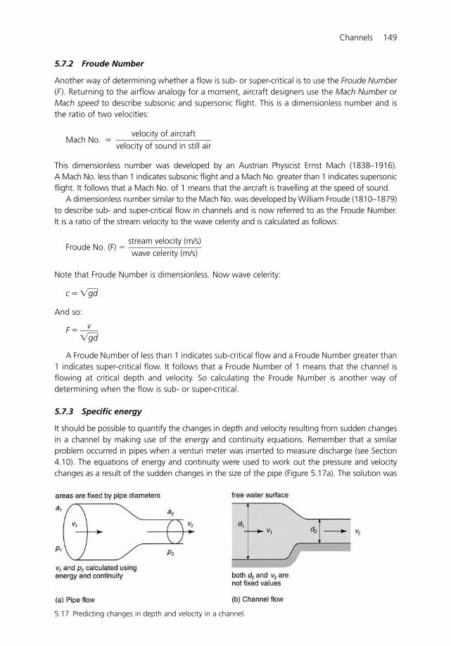
Channels 149
5.7.2 Froude Number
Another way of determining whether a flow is sub- or super-critical is to use the Froude Number(F ). Returning to the airflow analogy for a moment, aircraft designers use the Mach Number orMach speed to describe subsonic and supersonic flight. This is a dimensionless number and isthe ratio of two velocities:
This dimensionless number was developed by an Austrian Physicist Ernst Mach (1838–1916).A Mach No. less than 1 indicates subsonic flight and a Mach No. greater than 1 indicates supersonicflight. It follows that a Mach No. of 1 means that the aircraft is travelling at the speed of sound.
A dimensionless number similar to the Mach No. was developed by William Froude (1810–1879)to describe sub- and super-critical flow in channels and is now referred to as the Froude Number.It is a ratio of the stream velocity to the wave celerity and is calculated as follows:
Note that Froude Number is dimensionless. Now wave celerity:
And so:
A Froude Number of less than 1 indicates sub-critical flow and a Froude Number greater than1 indicates super-critical flow. It follows that a Froude Number of 1 means that the channel isflowing at critical depth and velocity. So calculating the Froude Number is another way ofdetermining when the flow is sub- or super-critical.
5.7.3 Specific energy
It should be possible to quantify the changes in depth and velocity resulting from sudden changesin a channel by making use of the energy and continuity equations. Remember that a similarproblem occurred in pipes when a venturi meter was inserted to measure discharge (see Section4.10). The equations of energy and continuity were used to work out the pressure and velocitychanges as a result of the sudden changes in the size of the pipe (Figure 5.17a). The solution was
F �v
�gd
c � �gd
Froude No. (F) � stream velocity (m/s)
wave celerity (m/s)
Mach No. � velocity of aircraft
velocity of sound in still air
5.17 Predicting changes in depth and velocity in a channel.
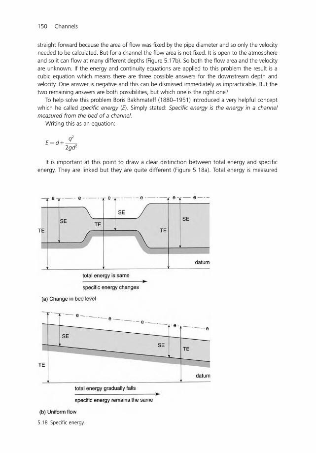
150 Channels
straight forward because the area of flow was fixed by the pipe diameter and so only the velocityneeded to be calculated. But for a channel the flow area is not fixed. It is open to the atmosphereand so it can flow at many different depths (Figure 5.17b). So both the flow area and the velocityare unknown. If the energy and continuity equations are applied to this problem the result is acubic equation which means there are three possible answers for the downstream depth andvelocity. One answer is negative and this can be dismissed immediately as impracticable. But thetwo remaining answers are both possibilities, but which one is the right one?
To help solve this problem Boris Bakhmateff (1880–1951) introduced a very helpful conceptwhich he called specific energy (E). Simply stated: Specific energy is the energy in a channelmeasured from the bed of a channel.
Writing this as an equation:
It is important at this point to draw a clear distinction between total energy and specificenergy. They are linked but they are quite different (Figure 5.18a). Total energy is measured
E � d�q2
2gd2
5.18 Specific energy.
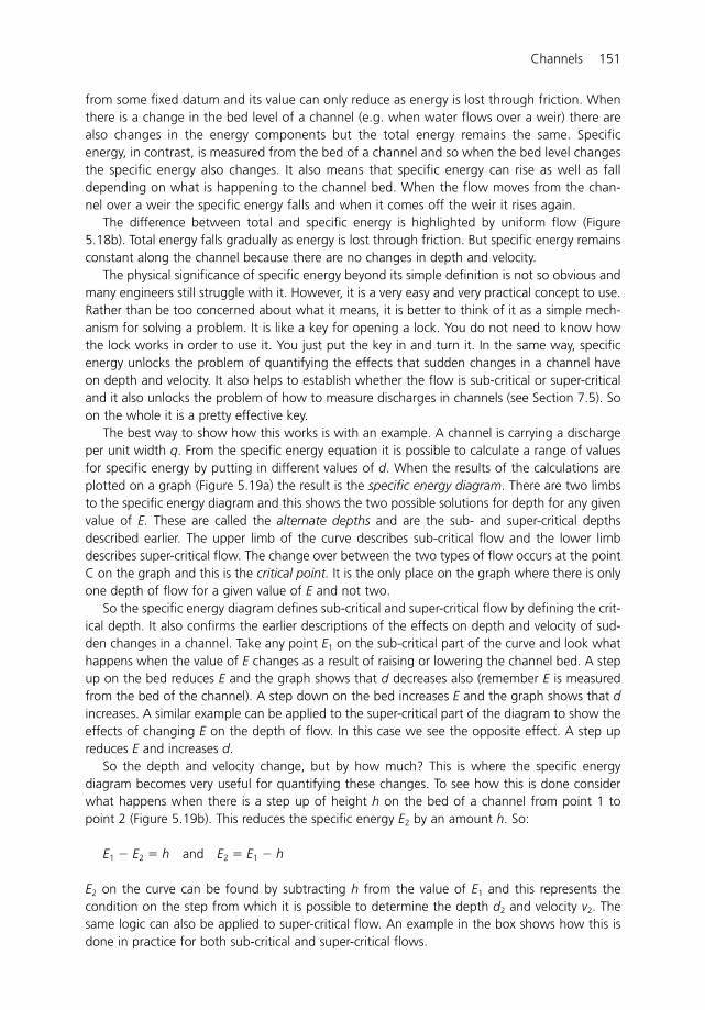
Channels 151
from some fixed datum and its value can only reduce as energy is lost through friction. Whenthere is a change in the bed level of a channel (e.g. when water flows over a weir) there arealso changes in the energy components but the total energy remains the same. Specificenergy, in contrast, is measured from the bed of a channel and so when the bed level changesthe specific energy also changes. It also means that specific energy can rise as well as falldepending on what is happening to the channel bed. When the flow moves from the chan-nel over a weir the specific energy falls and when it comes off the weir it rises again.
The difference between total and specific energy is highlighted by uniform flow (Figure5.18b). Total energy falls gradually as energy is lost through friction. But specific energy remainsconstant along the channel because there are no changes in depth and velocity.
The physical significance of specific energy beyond its simple definition is not so obvious andmany engineers still struggle with it. However, it is a very easy and very practical concept to use.Rather than be too concerned about what it means, it is better to think of it as a simple mech-anism for solving a problem. It is like a key for opening a lock. You do not need to know howthe lock works in order to use it. You just put the key in and turn it. In the same way, specificenergy unlocks the problem of quantifying the effects that sudden changes in a channel haveon depth and velocity. It also helps to establish whether the flow is sub-critical or super-criticaland it also unlocks the problem of how to measure discharges in channels (see Section 7.5). Soon the whole it is a pretty effective key.
The best way to show how this works is with an example. A channel is carrying a dischargeper unit width q. From the specific energy equation it is possible to calculate a range of valuesfor specific energy by putting in different values of d. When the results of the calculations areplotted on a graph (Figure 5.19a) the result is the specific energy diagram. There are two limbsto the specific energy diagram and this shows the two possible solutions for depth for any givenvalue of E. These are called the alternate depths and are the sub- and super-critical depthsdescribed earlier. The upper limb of the curve describes sub-critical flow and the lower limbdescribes super-critical flow. The change over between the two types of flow occurs at the pointC on the graph and this is the critical point. It is the only place on the graph where there is onlyone depth of flow for a given value of E and not two.
So the specific energy diagram defines sub-critical and super-critical flow by defining the crit-ical depth. It also confirms the earlier descriptions of the effects on depth and velocity of sud-den changes in a channel. Take any point E1 on the sub-critical part of the curve and look whathappens when the value of E changes as a result of raising or lowering the channel bed. A stepup on the bed reduces E and the graph shows that d decreases also (remember E is measuredfrom the bed of the channel). A step down on the bed increases E and the graph shows that dincreases. A similar example can be applied to the super-critical part of the diagram to show theeffects of changing E on the depth of flow. In this case we see the opposite effect. A step upreduces E and increases d.
So the depth and velocity change, but by how much? This is where the specific energydiagram becomes very useful for quantifying these changes. To see how this is done considerwhat happens when there is a step up of height h on the bed of a channel from point 1 topoint 2 (Figure 5.19b). This reduces the specific energy E2 by an amount h. So:
E1 � E2 � h and E2 � E1 � h
E2 on the curve can be found by subtracting h from the value of E1 and this represents thecondition on the step from which it is possible to determine the depth d2 and velocity v2. Thesame logic can also be applied to super-critical flow. An example in the box shows how this isdone in practice for both sub-critical and super-critical flows.
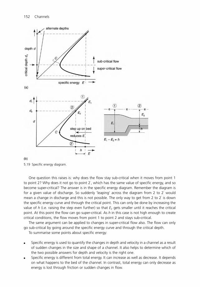
152 Channels
One question this raises is: why does the flow stay sub-critical when it moves from point 1to point 2? Why does it not go to point 2’, which has the same value of specific energy, and sobecome super-critical? The answer is in the specific energy diagram. Remember the diagram isfor a given value of discharge. So suddenly 'leaping' across the diagram from 2 to 2’ wouldmean a change in discharge and this is not possible. The only way to get from 2 to 2’ is downthe specific energy curve and through the critical point. This can only be done by increasing thevalue of h (i.e. raising the step even further) so that E2 gets smaller until it reaches the criticalpoint. At this point the flow can go super-critical. As h in this case is not high enough to createcritical conditions, the flow moves from point 1 to point 2 and stays sub-critical.
The same argument can be applied to changes in super-critical flow also. The flow can onlygo sub-critical by going around the specific energy curve and through the critical depth.
To summarise some points about specific energy:
� Specific energy is used to quantify the changes in depth and velocity in a channel as a resultof sudden changes in the size and shape of a channel. It also helps to determine which ofthe two possible answers for depth and velocity is the right one.
� Specific energy is different from total energy. It can increase as well as decrease. It dependson what happens to the bed of the channel. In contrast, total energy can only decrease asenergy is lost through friction or sudden changes in flow.
5.19 Specific energy diagram.
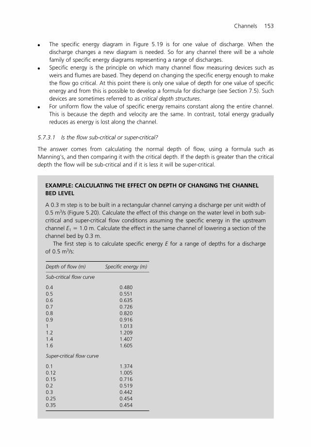
Channels 153
� The specific energy diagram in Figure 5.19 is for one value of discharge. When thedischarge changes a new diagram is needed. So for any channel there will be a wholefamily of specific energy diagrams representing a range of discharges.
� Specific energy is the principle on which many channel flow measuring devices such asweirs and flumes are based. They depend on changing the specific energy enough to makethe flow go critical. At this point there is only one value of depth for one value of specificenergy and from this is possible to develop a formula for discharge (see Section 7.5). Suchdevices are sometimes referred to as critical depth structures.
� For uniform flow the value of specific energy remains constant along the entire channel.This is because the depth and velocity are the same. In contrast, total energy graduallyreduces as energy is lost along the channel.
5.7.3.1 Is the flow sub-critical or super-critical?
The answer comes from calculating the normal depth of flow, using a formula such asManning's, and then comparing it with the critical depth. If the depth is greater than the criticaldepth the flow will be sub-critical and if it is less it will be super-critical.
EXAMPLE: CALCULATING THE EFFECT ON DEPTH OF CHANGING THE CHANNELBED LEVEL
A 0.3 m step is to be built in a rectangular channel carrying a discharge per unit width of0.5 m3/s (Figure 5.20). Calculate the effect of this change on the water level in both sub-critical and super-critical flow conditions assuming the specific energy in the upstreamchannel E1 � 1.0 m. Calculate the effect in the same channel of lowering a section of thechannel bed by 0.3 m.
The first step is to calculate specific energy E for a range of depths for a dischargeof 0.5 m3/s:
Depth of flow (m) Specific energy (m)
Sub-critical flow curve
0.4 0.4800.5 0.5510.6 0.6350.7 0.7260.8 0.8200.9 0.9161 1.0131.2 1.2091.4 1.4071.6 1.605
Super-critical flow curve
0.1 1.3740.12 1.0050.15 0.7160.2 0.5190.3 0.4420.25 0.4540.35 0.454
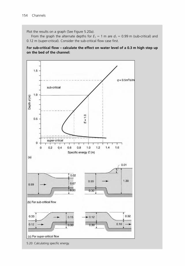
154 Channels
Plot the results on a graph (See Figure 5.20a).From the graph the alternate depths for E1 � 1 m are d1 � 0.99 m (sub-critical) and
0.12 m (super-critical). Consider the sub-critical flow case first.
For sub-critical flow – calculate the effect on water level of a 0.3 m high step upon the bed of the channel:
5.20 Calculating specific energy.
Channels 155
Specific energy in the channel is:
E1 � 1.0 m
And:
d1 � 0.99 m
Next calculate the specific energy on the step which is 0.3 m higher than the channel bed:
E2 � E1 � 0.3 � 0.7 m
Now locate E2 on the graph and read off the value for d2:
d2 � 0.67 m
Depth d2 is measured from the step and so the water level is 0.97 m above the originalchannel bed. This means that the water level has dropped 0.02 m as a result of raisingthe channel bed.
For sub-critical flow – calculate the effect on water level of a 0.3 m step down onthe bed of the channel:
Specific energy in the channel is:
E1 � 1.0 m
And:
d1 � 0.99 m
Next calculate the specific energy where the channel has been excavated by 0.3 m:
E2 � E1 � 0.3 � 1.3 m
Now locate E2 on the graph and read off the value for d2:
d2 � 1.30 m
Depth d2 is measured from the bed of the excavated section and so the water level is now1.30 m above the channel bed. This means that the water level rises by 0.01 m as a resultof the step down in the channel bed.
For super-critical flow – calculate the effect on water level of a 0.3 m step up onthe bed of the channel:
Specific energy in the channel is:
E1 � 1.0 m
And:
d1 � 0.12 m
Next calculate the specific energy on the step which is 0.3 m higher than the channel bed:
E2 � E1 � 0.3 � 0.7 m
156 Channels
Now locate E2 on the graph and read off the value for d2:
d2 � 0.15 m
Now depth d2 is measured from the top of the raised bed and so the water level is now0.45 m above the original channel bed. This means that the water level rises 0.33 m as aresult of raising the channel bed.
For super-critical flow – calculate the effect on water level of a 0.3 m step downon the bed of the channel:
Specific energy in the channel is:
E1 � 1.0 m
And:
d1 � 0.12 m
Next calculate the specific energy where the channel has been excavated by 0.3 m:
E2 � E1 � 0.3 � 1.3 m
Now locate E2 on the graph and read off the value for d2:
d2 � 0.10 m
Now depth d2 is measured from the bed of the excavated bed and so the water level isnow 0.20 m below the original channel bed. This means that the water level drops0.32 m as a result of the step down in the channel bed.
5.7.4 Critical depth
The critical depth dc can be determined directly from the specific energy diagram but it canbe difficult to locate its exact position because of the rounded shape of the curve close to thecritical point. To overcome this problem it can be calculated using a formula derived from thespecific energy equation:
This formula shows that the critical depth is influenced only by the discharge per unit widthq. It has nothing to do with the slope or the normal depth. For the mathematically minded aproof of this is given in the box.
dc � 3� q2
g
DERIVATION: CRITICAL DEPTH EQUATION
Derive a formula for the critical depth and its location on the specific energy diagram(Figure 5.20).
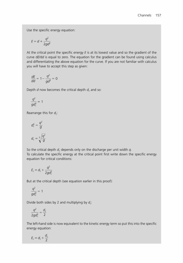
Channels 157
Use the specific energy equation:
At the critical point the specific energy E is at its lowest value and so the gradient of thecurve dE/dd is equal to zero. The equation for the gradient can be found using calculusand differentiating the above equation for the curve. If you are not familiar with calculusyou will have to accept this step as given:
Depth d now becomes the critical depth dc and so:
Rearrange this for dc:
So the critical depth dc depends only on the discharge per unit width q.To calculate the specific energy at the critical point first write down the specific energyequation for critical conditions:
But at the critical depth (see equation earlier in this proof):
Divide both sides by 2 and multiplying by dc:
The left-hand side is now equivalent to the kinetic energy term so put this into the specificenergy equation:
Ec � dc
�
dc
2
q2
2gdc2 �
dc
2
q2
gdc3 � 1
Ec � dc
�
q2
2gdc2
dc � 3�q2
g
d3c �
q2
g
q2
gdc3 � 1
dEdd
� 1� q2
gd3 � 0
E � d �
q2
2gd2
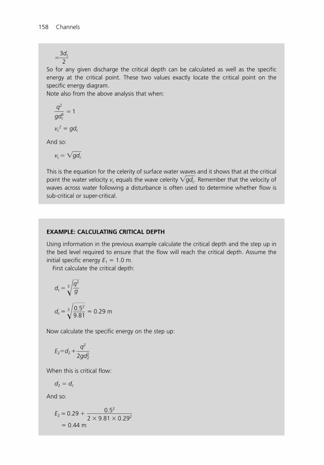
158 Channels
So for any given discharge the critical depth can be calculated as well as the specificenergy at the critical point. These two values exactly locate the critical point on thespecific energy diagram.Note also from the above analysis that when:
vc2 � gdc
And so:
This is the equation for the celerity of surface water waves and it shows that at the criticalpoint the water velocity vc equals the wave celerity . Remember that the velocity ofwaves across water following a disturbance is often used to determine whether flow issub-critical or super-critical.
�gdc
vc � �gdc
q2
gdc3 � 1
�3dc
2
EXAMPLE: CALCULATING CRITICAL DEPTH
Using information in the previous example calculate the critical depth and the step up inthe bed level required to ensure that the flow will reach the critical depth. Assume theinitial specific energy E1 � 1.0 m.
First calculate the critical depth:
Now calculate the specific energy on the step up:
When this is critical flow:
d2 � dc
And so:
� 0.44 m
E2 � 0.29 �
0.52
2 � 9.81 � 0.292
E2�d2 �q2
2gd22
dc � 3�0.52
9.81 � 0.29 m
dc � 3�q2
g
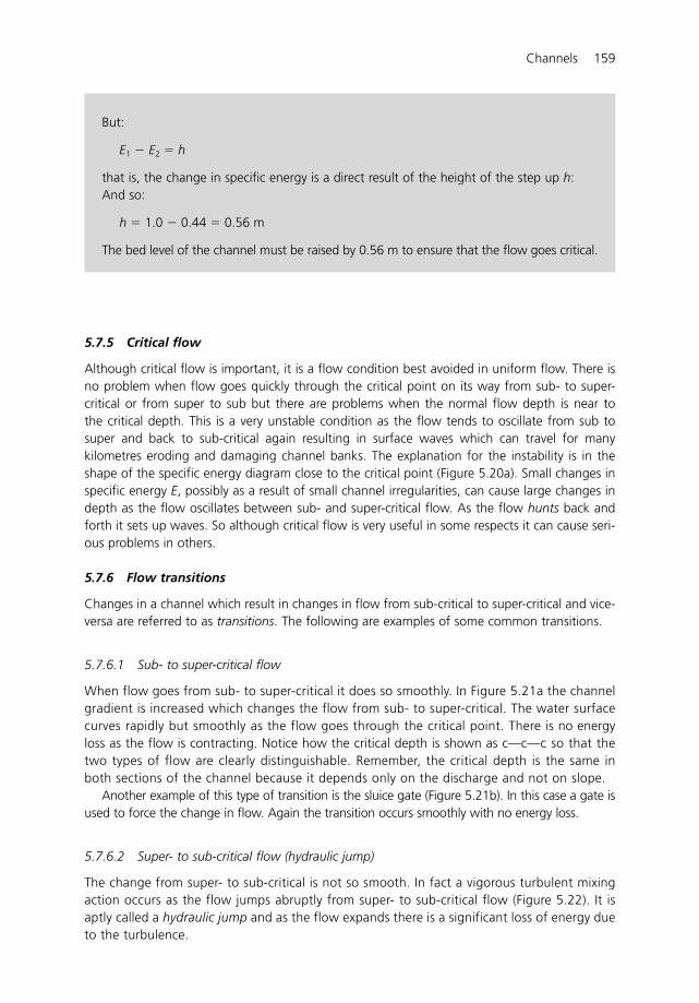
Channels 159
5.7.5 Critical flow
Although critical flow is important, it is a flow condition best avoided in uniform flow. There isno problem when flow goes quickly through the critical point on its way from sub- to super-critical or from super to sub but there are problems when the normal flow depth is near tothe critical depth. This is a very unstable condition as the flow tends to oscillate from sub tosuper and back to sub-critical again resulting in surface waves which can travel for manykilometres eroding and damaging channel banks. The explanation for the instability is in theshape of the specific energy diagram close to the critical point (Figure 5.20a). Small changes inspecific energy E, possibly as a result of small channel irregularities, can cause large changes indepth as the flow oscillates between sub- and super-critical flow. As the flow hunts back andforth it sets up waves. So although critical flow is very useful in some respects it can cause seri-ous problems in others.
5.7.6 Flow transitions
Changes in a channel which result in changes in flow from sub-critical to super-critical and vice-versa are referred to as transitions. The following are examples of some common transitions.
5.7.6.1 Sub- to super-critical flow
When flow goes from sub- to super-critical it does so smoothly. In Figure 5.21a the channelgradient is increased which changes the flow from sub- to super-critical. The water surfacecurves rapidly but smoothly as the flow goes through the critical point. There is no energyloss as the flow is contracting. Notice how the critical depth is shown as c—c—c so that thetwo types of flow are clearly distinguishable. Remember, the critical depth is the same inboth sections of the channel because it depends only on the discharge and not on slope.
Another example of this type of transition is the sluice gate (Figure 5.21b). In this case a gate isused to force the change in flow. Again the transition occurs smoothly with no energy loss.
5.7.6.2 Super- to sub-critical flow (hydraulic jump)
The change from super- to sub-critical is not so smooth. In fact a vigorous turbulent mixingaction occurs as the flow jumps abruptly from super- to sub-critical flow (Figure 5.22). It isaptly called a hydraulic jump and as the flow expands there is a significant loss of energy dueto the turbulence.
But:
E1 � E2 � h
that is, the change in specific energy is a direct result of the height of the step up h:And so:
h � 1.0 � 0.44 � 0.56 m
The bed level of the channel must be raised by 0.56 m to ensure that the flow goes critical.
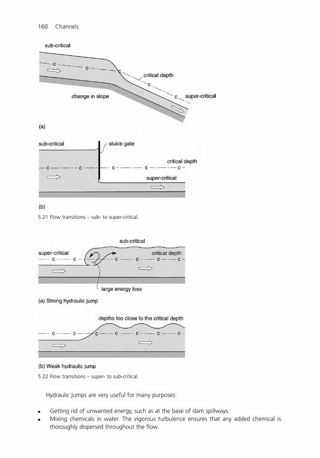
160 Channels
5.21 Flow transitions – sub- to super-critical.
5.22 Flow transitions – super- to sub-critical.
Hydraulic jumps are very useful for many purposes:
� Getting rid of unwanted energy, such as at the base of dam spillways.� Mixing chemicals in water. The vigorous turbulence ensures that any added chemical is
thoroughly dispersed throughout the flow.
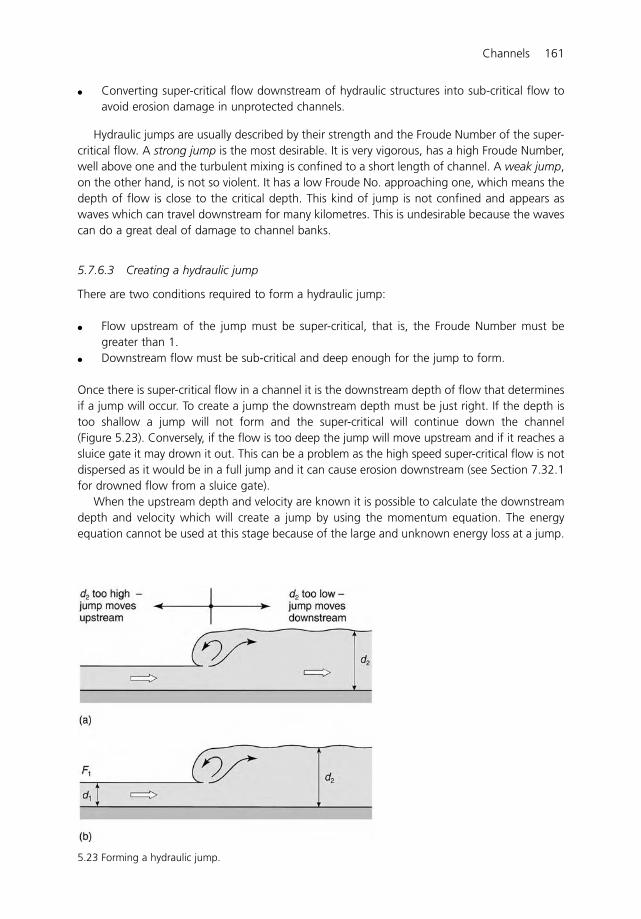
Channels 161
5.23 Forming a hydraulic jump.
� Converting super-critical flow downstream of hydraulic structures into sub-critical flow toavoid erosion damage in unprotected channels.
Hydraulic jumps are usually described by their strength and the Froude Number of the super-critical flow. A strong jump is the most desirable. It is very vigorous, has a high Froude Number,well above one and the turbulent mixing is confined to a short length of channel. A weak jump,on the other hand, is not so violent. It has a low Froude No. approaching one, which means thedepth of flow is close to the critical depth. This kind of jump is not confined and appears aswaves which can travel downstream for many kilometres. This is undesirable because the wavescan do a great deal of damage to channel banks.
5.7.6.3 Creating a hydraulic jump
There are two conditions required to form a hydraulic jump:
� Flow upstream of the jump must be super-critical, that is, the Froude Number must begreater than 1.
� Downstream flow must be sub-critical and deep enough for the jump to form.
Once there is super-critical flow in a channel it is the downstream depth of flow that determinesif a jump will occur. To create a jump the downstream depth must be just right. If the depth istoo shallow a jump will not form and the super-critical will continue down the channel(Figure 5.23). Conversely, if the flow is too deep the jump will move upstream and if it reaches asluice gate it may drown it out. This can be a problem as the high speed super-critical flow is notdispersed as it would be in a full jump and it can cause erosion downstream (see Section 7.32.1for drowned flow from a sluice gate).
When the upstream depth and velocity are known it is possible to calculate the downstreamdepth and velocity which will create a jump by using the momentum equation. The energyequation cannot be used at this stage because of the large and unknown energy loss at a jump.
162 Channels
The formula is derived from the momentum equation which links the two depths of flowd1 and d2:
Where d1 is upstream depth; d2 is downstream depth; F1 is upstream Froude No.Most hydraulic jump problems involve calculating the downstream depth d2 in order to
determine the conditions under which a jump will occur. But determining a value for d2 is finein theory, but in practice the formation of a jump is very sensitive to the downstream depth. Thismeans that when the downstream depth is a little more or less than the calculated value, thejump does not stabilise at the selected location but moves up and down the channel huntingfor the right depth of flow. In practice it is very difficult to control water depths with greataccuracy and so some method is needed to remove the sensitivity of the jump to downstreamwater level and so stabilise it. This is the job of a stilling basin which is a concrete apron locateddownstream of a weir or sluice gate. Its primary job is to dissipate unwanted energy to protectthe downstream channel and it does this by making sure the hydraulic jump forms on theconcrete slab even though the downstream water level may vary considerably. This is discussedfurther in Section 7.10.
5.7.6.4 Calculating energy losses
Once the downstream depth and velocity have been calculated using the momentum equation,the loss of energy at a jump can be determined using the total energy equation as follows:
Total energy upstream � total energy downstream � energy loss at jump
That is:
d1
�
v21
2g � z1 � d2
�
v22
2g � z2
�
losses
d2
d1 � 1
2 ��1�8F2
1 �1�
EXAMPLE: CALCULATING THE DOWNSTREAM DEPTH TO FORMA HYDRAULIC JUMP
Calculate the depth required downstream to create the jump in a channel carrying adischarge of 0.8 m3/s per m width at a depth of 0.25 m.The downstream depth can be calculated using the formula:
First calculate the velocity using the discharge equation:
q � v1d1
v1 �0.8
0.25� 3.2 m/s
d2
d1�
12
��1�8F21�1�
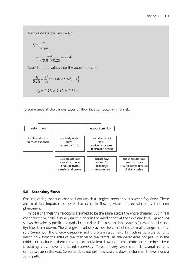
Channels 163
To summarise all the various types of flow that can occur in channels:
Next calculate the Froude No:
Substitute the values into the above formula:
d2 � 0.25 � 2.43 � 0.61 m
d2
0.25�
12��1�(8�2.042)�1�
�3.2
�9.81�0.25� 2.04
Fi �v1
�gd1
basis of designfor most channels
uniform flow
gradually-variedflow –
caused by friction
sub-critical flow– most commonin natural rivers,
canals, and drains
critical flow– used fordischarge
measurement
super-critical flowrarely occurs –
only spillways and d/sof sluice gates
rapidly-variedflow –
sudden changesin size and shape
non-uniform flow
5.8 Secondary flows
One interesting aspect of channel flow (which all anglers know about) is secondary flows. Theseare small but important currents that occur in flowing water and explain many importantphenomena.
In ideal channels the velocity is assumed to be the same across the entire channel. But in realchannels the velocity is usually much higher in the middle than at the sides and bed. Figure 5.24shows the velocity profile in a typical channel and in cross section, isotachs (lines of equal veloc-ity) have been drawn. The changes in velocity across the channel cause small changes in pres-sure (remember the energy equation) and these are responsible for setting up cross currentswhich flow from the sides of the channel to the centre. As the water does not pile up in themiddle of a channel there must be an equivalent flow from the centre to the edge. Thesecirculating cross flows are called secondary flows. In very wide channels several currentscan be set up in this way. So water does not just flow straight down a channel, it flows along aspiral path.
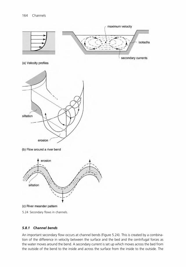
164 Channels
5.8.1 Channel bends
An important secondary flow occurs at channel bends (Figure 5.24). This is created by a combina-tion of the difference in velocity between the surface and the bed and the centrifugal forces asthe water moves around the bend. A secondary current is set up which moves across the bed fromthe outside of the bend to the inside and across the surface from the inside to the outside. The
5.24 Secondary flows in channels.
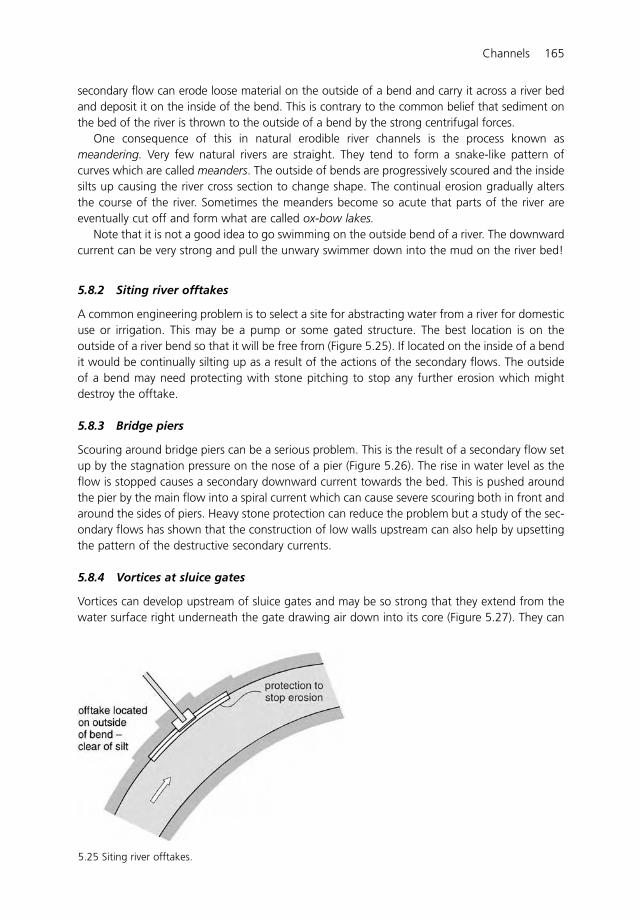
Channels 165
5.25 Siting river offtakes.
secondary flow can erode loose material on the outside of a bend and carry it across a river bedand deposit it on the inside of the bend. This is contrary to the common belief that sediment onthe bed of the river is thrown to the outside of a bend by the strong centrifugal forces.
One consequence of this in natural erodible river channels is the process known asmeandering. Very few natural rivers are straight. They tend to form a snake-like pattern ofcurves which are called meanders. The outside of bends are progressively scoured and the insidesilts up causing the river cross section to change shape. The continual erosion gradually altersthe course of the river. Sometimes the meanders become so acute that parts of the river areeventually cut off and form what are called ox-bow lakes.
Note that it is not a good idea to go swimming on the outside bend of a river. The downwardcurrent can be very strong and pull the unwary swimmer down into the mud on the river bed!
5.8.2 Siting river offtakes
A common engineering problem is to select a site for abstracting water from a river for domesticuse or irrigation. This may be a pump or some gated structure. The best location is on theoutside of a river bend so that it will be free from (Figure 5.25). If located on the inside of a bendit would be continually silting up as a result of the actions of the secondary flows. The outsideof a bend may need protecting with stone pitching to stop any further erosion which mightdestroy the offtake.
5.8.3 Bridge piers
Scouring around bridge piers can be a serious problem. This is the result of a secondary flow setup by the stagnation pressure on the nose of a pier (Figure 5.26). The rise in water level as theflow is stopped causes a secondary downward current towards the bed. This is pushed aroundthe pier by the main flow into a spiral current which can cause severe scouring both in front andaround the sides of piers. Heavy stone protection can reduce the problem but a study of the sec-ondary flows has shown that the construction of low walls upstream can also help by upsettingthe pattern of the destructive secondary currents.
5.8.4 Vortices at sluice gates
Vortices can develop upstream of sluice gates and may be so strong that they extend from thewater surface right underneath the gate drawing air down into its core (Figure 5.27). They can
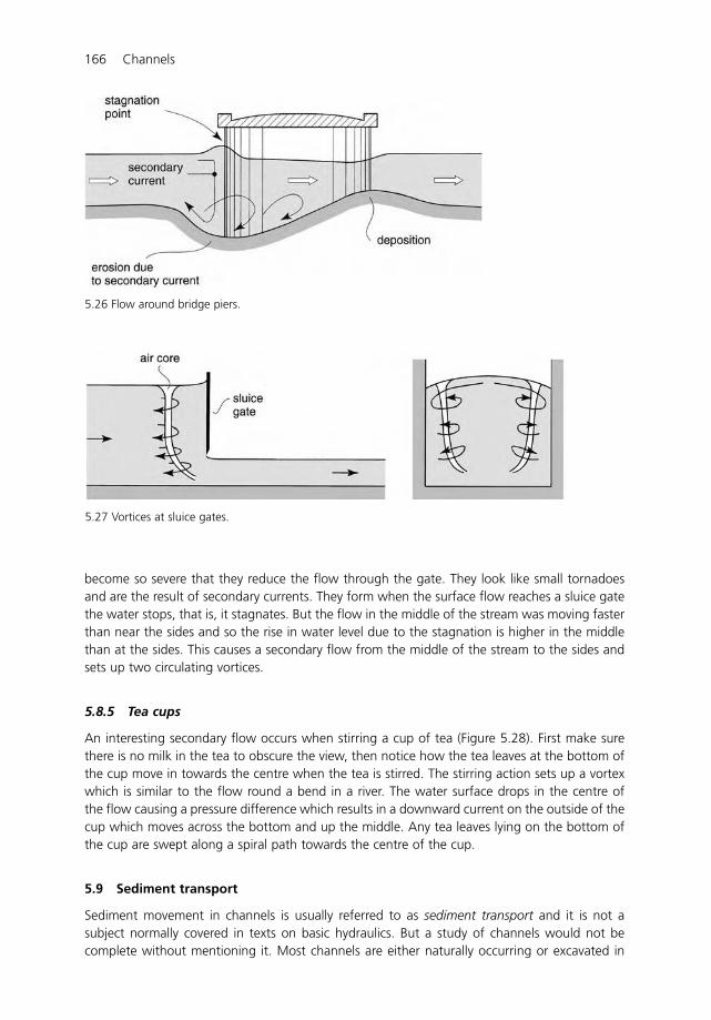
166 Channels
become so severe that they reduce the flow through the gate. They look like small tornadoesand are the result of secondary currents. They form when the surface flow reaches a sluice gatethe water stops, that is, it stagnates. But the flow in the middle of the stream was moving fasterthan near the sides and so the rise in water level due to the stagnation is higher in the middlethan at the sides. This causes a secondary flow from the middle of the stream to the sides andsets up two circulating vortices.
5.8.5 Tea cups
An interesting secondary flow occurs when stirring a cup of tea (Figure 5.28). First make surethere is no milk in the tea to obscure the view, then notice how the tea leaves at the bottom ofthe cup move in towards the centre when the tea is stirred. The stirring action sets up a vortexwhich is similar to the flow round a bend in a river. The water surface drops in the centre ofthe flow causing a pressure difference which results in a downward current on the outside of thecup which moves across the bottom and up the middle. Any tea leaves lying on the bottom ofthe cup are swept along a spiral path towards the centre of the cup.
5.9 Sediment transport
Sediment movement in channels is usually referred to as sediment transport and it is not asubject normally covered in texts on basic hydraulics. But a study of channels would not becomplete without mentioning it. Most channels are either naturally occurring or excavated in
5.26 Flow around bridge piers.
5.27 Vortices at sluice gates.
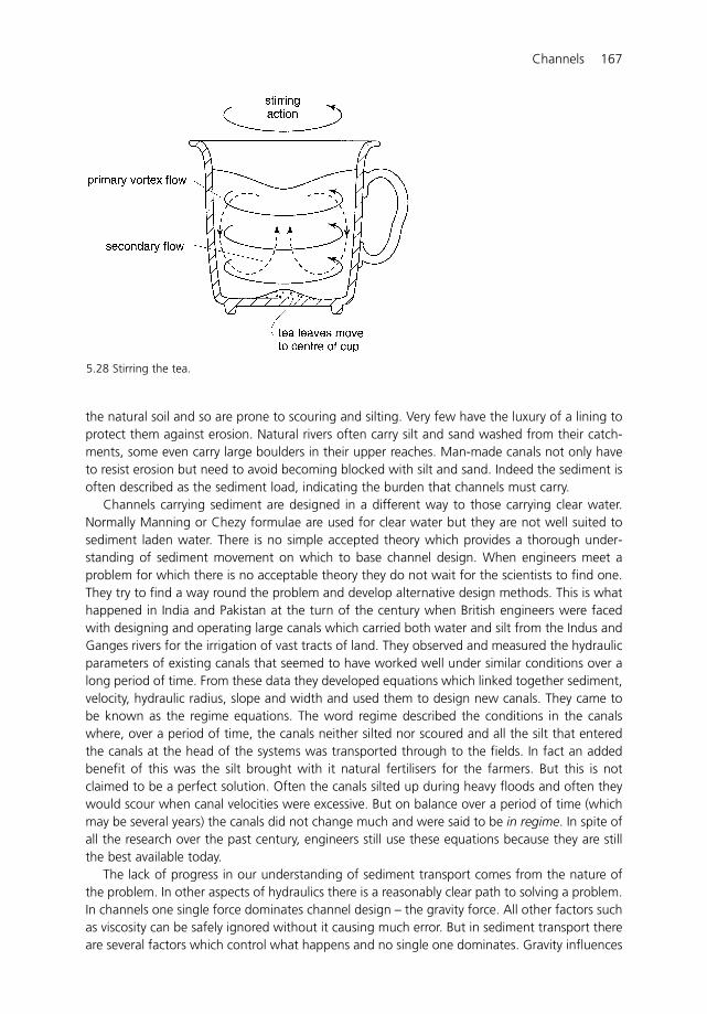
Channels 167
the natural soil and so are prone to scouring and silting. Very few have the luxury of a lining toprotect them against erosion. Natural rivers often carry silt and sand washed from their catch-ments, some even carry large boulders in their upper reaches. Man-made canals not only haveto resist erosion but need to avoid becoming blocked with silt and sand. Indeed the sediment isoften described as the sediment load, indicating the burden that channels must carry.
Channels carrying sediment are designed in a different way to those carrying clear water.Normally Manning or Chezy formulae are used for clear water but they are not well suited tosediment laden water. There is no simple accepted theory which provides a thorough under-standing of sediment movement on which to base channel design. When engineers meet aproblem for which there is no acceptable theory they do not wait for the scientists to find one.They try to find a way round the problem and develop alternative design methods. This is whathappened in India and Pakistan at the turn of the century when British engineers were facedwith designing and operating large canals which carried both water and silt from the Indus andGanges rivers for the irrigation of vast tracts of land. They observed and measured the hydraulicparameters of existing canals that seemed to have worked well under similar conditions over along period of time. From these data they developed equations which linked together sediment,velocity, hydraulic radius, slope and width and used them to design new canals. They came tobe known as the regime equations. The word regime described the conditions in the canalswhere, over a period of time, the canals neither silted nor scoured and all the silt that enteredthe canals at the head of the systems was transported through to the fields. In fact an addedbenefit of this was the silt brought with it natural fertilisers for the farmers. But this is notclaimed to be a perfect solution. Often the canals silted up during heavy floods and often theywould scour when canal velocities were excessive. But on balance over a period of time (whichmay be several years) the canals did not change much and were said to be in regime. In spite ofall the research over the past century, engineers still use these equations because they are stillthe best available today.
The lack of progress in our understanding of sediment transport comes from the nature ofthe problem. In other aspects of hydraulics there is a reasonably clear path to solving a problem.In channels one single force dominates channel design – the gravity force. All other factors suchas viscosity can be safely ignored without it causing much error. But in sediment transport thereare several factors which control what happens and no single one dominates. Gravity influences
5.28 Stirring the tea.
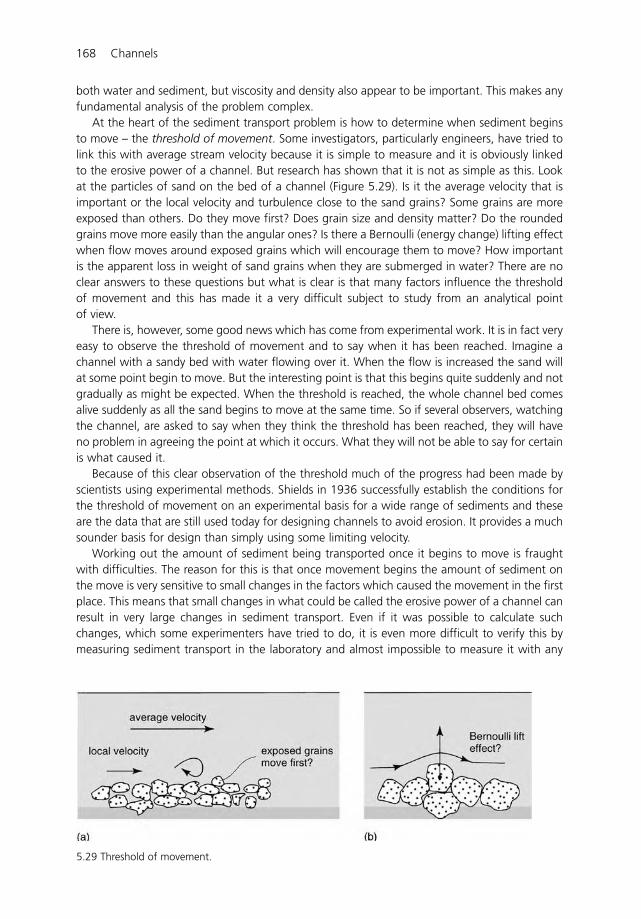
168 Channels
both water and sediment, but viscosity and density also appear to be important. This makes anyfundamental analysis of the problem complex.
At the heart of the sediment transport problem is how to determine when sediment beginsto move – the threshold of movement. Some investigators, particularly engineers, have tried tolink this with average stream velocity because it is simple to measure and it is obviously linkedto the erosive power of a channel. But research has shown that it is not as simple as this. Lookat the particles of sand on the bed of a channel (Figure 5.29). Is it the average velocity that isimportant or the local velocity and turbulence close to the sand grains? Some grains are moreexposed than others. Do they move first? Does grain size and density matter? Do the roundedgrains move more easily than the angular ones? Is there a Bernoulli (energy change) lifting effectwhen flow moves around exposed grains which will encourage them to move? How importantis the apparent loss in weight of sand grains when they are submerged in water? There are noclear answers to these questions but what is clear is that many factors influence the thresholdof movement and this has made it a very difficult subject to study from an analytical pointof view.
There is, however, some good news which has come from experimental work. It is in fact veryeasy to observe the threshold of movement and to say when it has been reached. Imagine achannel with a sandy bed with water flowing over it. When the flow is increased the sand willat some point begin to move. But the interesting point is that this begins quite suddenly and notgradually as might be expected. When the threshold is reached, the whole channel bed comesalive suddenly as all the sand begins to move at the same time. So if several observers, watchingthe channel, are asked to say when they think the threshold has been reached, they will haveno problem in agreeing the point at which it occurs. What they will not be able to say for certainis what caused it.
Because of this clear observation of the threshold much of the progress had been made byscientists using experimental methods. Shields in 1936 successfully establish the conditions forthe threshold of movement on an experimental basis for a wide range of sediments and theseare the data that are still used today for designing channels to avoid erosion. It provides a muchsounder basis for design than simply using some limiting velocity.
Working out the amount of sediment being transported once it begins to move is fraughtwith difficulties. The reason for this is that once movement begins the amount of sediment onthe move is very sensitive to small changes in the factors which caused the movement in the firstplace. This means that small changes in what could be called the erosive power of a channel canresult in very large changes in sediment transport. Even if it was possible to calculate suchchanges, which some experimenters have tried to do, it is even more difficult to verify this bymeasuring sediment transport in the laboratory and almost impossible to measure it with any
5.29 Threshold of movement.
Channels 169
accuracy in the field. For these reasons it seems unlikely that there will be any significantimprovements in the predictions of sediment transport and that engineers will have to rely onthe regime equations for some time to come.
5.10 Some examples to test your understanding
1 An open channel of rectangular section has a bed width of 1.0 m. If the channel carries adischarge 1.0 m3/s calculate the depth of flow when the Manning's roughness coefficientis 0.015 and the bed slope is 1 in 1000. Calculate the Froude Number in the channel andthe critical depth (0.5 m; 0.45 m; 0.29 m).
2 A rectangular channel of bed width 2.5 m carries a discharge of 1.75 m3/s. Calculate thenormal depth of flow when the Chezy coefficient is 60 and the slope is 1 in 2000. Calculatethe critical depth and say whether the flow is sub-critical or super-critical (0.75 m; 0.37 m;flow is sub-critical).
3 A trapezoidal channel is to be designed and constructed in a sandy loam with a longitudinalslope of 1 in 5000 to carry a discharge of 2.3 m3/s. Calculate suitable dimensions for thedepth and bed width assuming Manning's n is 0.022 and the side slope is 1 in 2 (d � 0.98 m;b � 2.94 m (b � 3d)).
4 A trapezoidal channel carrying a discharge of 0.75 m3/s is to be lined with concrete to avoidseepage problems. Calculate the channels dimensions which will minimise the amount ofconcrete when Manning's n for concrete is 0.015 and the channel slope is 1 in 1250 (for ahexagonal channel d � 0.37 m; b � 0.8 m. Note that other answers are possible dependingon choice of side slope).
5 A hydraulic jump occurs in a rectangular channel 2.3 m wide when the discharge is1.5 m3/s. If the upstream depth is 0.25 m calculate the upstream Froude Number, the depthof flow downstream of the jump and the energy loss in the jump (2.78 m; 0.87 m; 0.3 m).
6 Waves
6.1 Introduction
Waves are very familiar to everyone, particularly those that toss about at sea during windy,stormy weather and those which roll in rhythmically on the beach. The tides too are wavesbut they are not so obvious as they slowly build up and subside twice a day and move manymillions of tonnes of water across the oceans. But waves are not just confined to the sea.Earlier, in Chapter 5, waves were described on a still pond and on a flowing stream when astone was thrown into the water to help determine critical flow conditions. Surge waves cansometimes be seen in rivers when control gates are suddenly closed and during high tideswhen tidal bores, some of which are quite famous, travel upstream from the mouth of rivers.Floods flowing down rivers too are another kind of wave which can be several hundreds ofkilometres long.
Waves in rivers depend on gravity for their shape and size in much the same way thatchannels themselves depend on the force of gravity down the land slope for their energy. Seawaves are different as they depend on the circulation of the atmosphere and the resulting windsfor their energy. Although it is possible for winds to create waves on lakes, they are not usuallyas large as those which can be generated by strong winds blowing over vast stretches of theoceans. These are the waves which play a large part in shaping our shorelines.
Sea waves tend to affect only the water surface. Indeed wave movement is different fromthe movement of the water in which it is travelling. Watching a single wave, it seems totravel a great distance at a steady speed. But observing the water closely, it hardly moves atall. Just look at any object floating – a seagull – on the water surface to appreciate this.When a wave passes the bird is not swept along with the wave it just bobs up and down.Leonardo da Vinci (1452–1519) compared water waves with the waves you see when thewind blows across a field of corn. The wave pattern seems to travel across the entire fieldand yet individual stalks only sway back and forth. Another example is that of a rope whichis held at one end and shaken. A wave pattern travels along the rope but the rope onlymoves up and down. So if the water (or the corn or rope) is not being transported thenwhat is? The answer is energy. It is energy which is being transported across the water andthrough the corn and along the rope.
Our understanding of waves and how they are generated is far from complete. This isbecause is it difficult to observe waves at sea and also because all the mathematical formulaeare based on ideal fluids and the sea does not always fit in with the ideal.
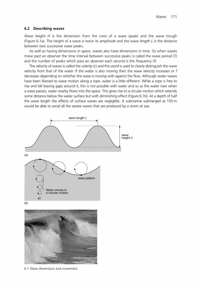
Waves 171
6.2 Describing waves
Wave height H is the dimension from the crest of a wave (peak) and the wave trough(Figure 6.1a). The height of a wave is twice its amplitude and the wave length L is the distancebetween two successive wave peaks.
As well as having dimensions in space, waves also have dimensions in time. So when wavesmove past an observer the time interval between successive peaks is called the wave period (T)and the number of peaks which pass an observer each second is the frequency (f).
The velocity of waves is called the celerity (c) and this word is used to clearly distinguish the wavevelocity from that of the water. If the water is also moving then the wave velocity increases or fdecreases depending on whether the wave is moving with against the flow. Although water waveshave been likened to wave motion along a rope, water is a little different. While a rope is free torise and fall leaving gaps around it, this is not possible with water and so as the water rises whena wave passes, water nearby flows into the space. This gives rise to a circular motion which extendssome distance below the water surface but with diminishing effect (Figure 6.1b). At a depth of halfthe wave length the effects of surface waves are negligible. A submarine submerged at 150 mwould be able to avoid all the severe waves that are produced by a storm at sea.
wave length L
waveheight H
(b)
(a)
wave pattern
Water moves ina circular motion
6.1 Wave dimensions and movement.
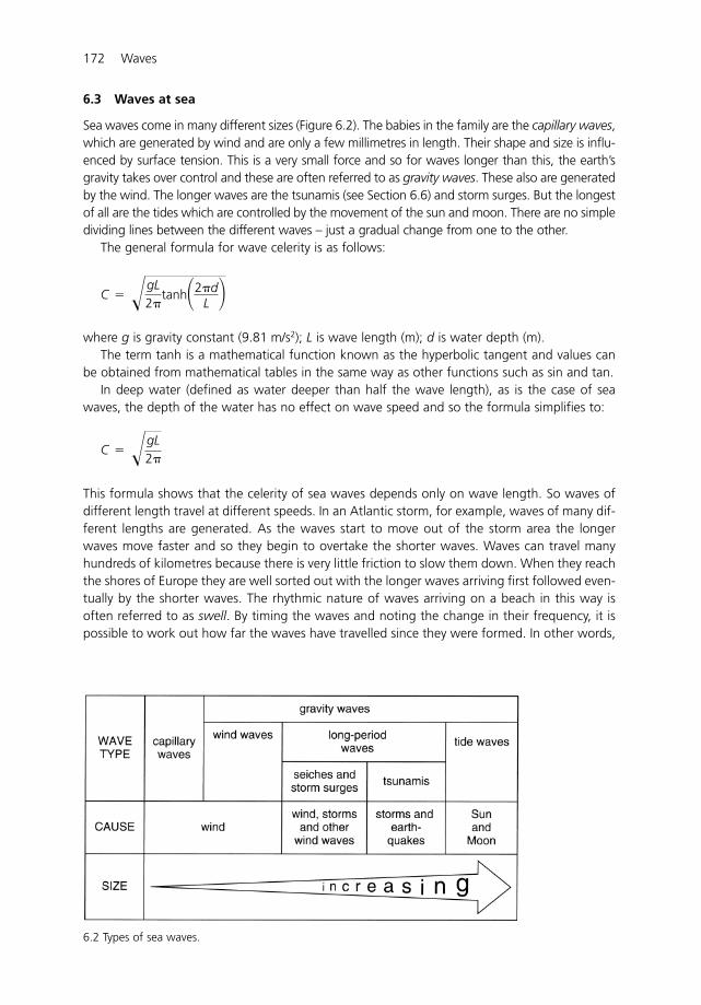
172 Waves
6.3 Waves at sea
Sea waves come in many different sizes (Figure 6.2). The babies in the family are the capillary waves,which are generated by wind and are only a few millimetres in length. Their shape and size is influ-enced by surface tension. This is a very small force and so for waves longer than this, the earth’sgravity takes over control and these are often referred to as gravity waves. These also are generatedby the wind. The longer waves are the tsunamis (see Section 6.6) and storm surges. But the longestof all are the tides which are controlled by the movement of the sun and moon. There are no simpledividing lines between the different waves – just a gradual change from one to the other.
The general formula for wave celerity is as follows:
where g is gravity constant (9.81 m/s2); L is wave length (m); d is water depth (m).The term tanh is a mathematical function known as the hyperbolic tangent and values can
be obtained from mathematical tables in the same way as other functions such as sin and tan.In deep water (defined as water deeper than half the wave length), as is the case of sea
waves, the depth of the water has no effect on wave speed and so the formula simplifies to:
This formula shows that the celerity of sea waves depends only on wave length. So waves ofdifferent length travel at different speeds. In an Atlantic storm, for example, waves of many dif-ferent lengths are generated. As the waves start to move out of the storm area the longerwaves move faster and so they begin to overtake the shorter waves. Waves can travel manyhundreds of kilometres because there is very little friction to slow them down. When they reachthe shores of Europe they are well sorted out with the longer waves arriving first followed even-tually by the shorter waves. The rhythmic nature of waves arriving on a beach in this way isoften referred to as swell. By timing the waves and noting the change in their frequency, it ispossible to work out how far the waves have travelled since they were formed. In other words,
C � �gL2�
C � �gL2�
tanh�2�dL �
6.2 Types of sea waves.
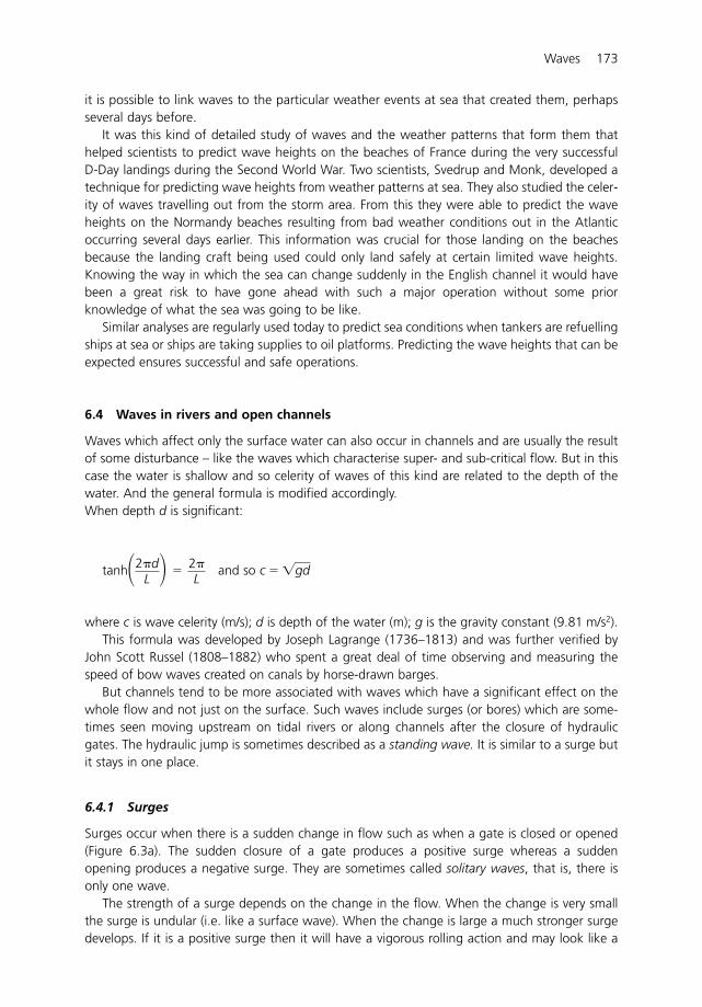
Waves 173
it is possible to link waves to the particular weather events at sea that created them, perhapsseveral days before.
It was this kind of detailed study of waves and the weather patterns that form them thathelped scientists to predict wave heights on the beaches of France during the very successfulD-Day landings during the Second World War. Two scientists, Svedrup and Monk, developed atechnique for predicting wave heights from weather patterns at sea. They also studied the celer-ity of waves travelling out from the storm area. From this they were able to predict the waveheights on the Normandy beaches resulting from bad weather conditions out in the Atlanticoccurring several days earlier. This information was crucial for those landing on the beachesbecause the landing craft being used could only land safely at certain limited wave heights.Knowing the way in which the sea can change suddenly in the English channel it would havebeen a great risk to have gone ahead with such a major operation without some priorknowledge of what the sea was going to be like.
Similar analyses are regularly used today to predict sea conditions when tankers are refuellingships at sea or ships are taking supplies to oil platforms. Predicting the wave heights that can beexpected ensures successful and safe operations.
6.4 Waves in rivers and open channels
Waves which affect only the surface water can also occur in channels and are usually the resultof some disturbance – like the waves which characterise super- and sub-critical flow. But in thiscase the water is shallow and so celerity of waves of this kind are related to the depth of thewater. And the general formula is modified accordingly.When depth d is significant:
and so
where c is wave celerity (m/s); d is depth of the water (m); g is the gravity constant (9.81 m/s2).This formula was developed by Joseph Lagrange (1736–1813) and was further verified by
John Scott Russel (1808–1882) who spent a great deal of time observing and measuring thespeed of bow waves created on canals by horse-drawn barges.
But channels tend to be more associated with waves which have a significant effect on thewhole flow and not just on the surface. Such waves include surges (or bores) which are some-times seen moving upstream on tidal rivers or along channels after the closure of hydraulicgates. The hydraulic jump is sometimes described as a standing wave. It is similar to a surge butit stays in one place.
6.4.1 Surges
Surges occur when there is a sudden change in flow such as when a gate is closed or opened(Figure 6.3a). The sudden closure of a gate produces a positive surge whereas a suddenopening produces a negative surge. They are sometimes called solitary waves, that is, there isonly one wave.
The strength of a surge depends on the change in the flow. When the change is very smallthe surge is undular (i.e. like a surface wave). When the change is large a much stronger surgedevelops. If it is a positive surge then it will have a vigorous rolling action and may look like a
c � �gdtanh�2�dL � �
2�L
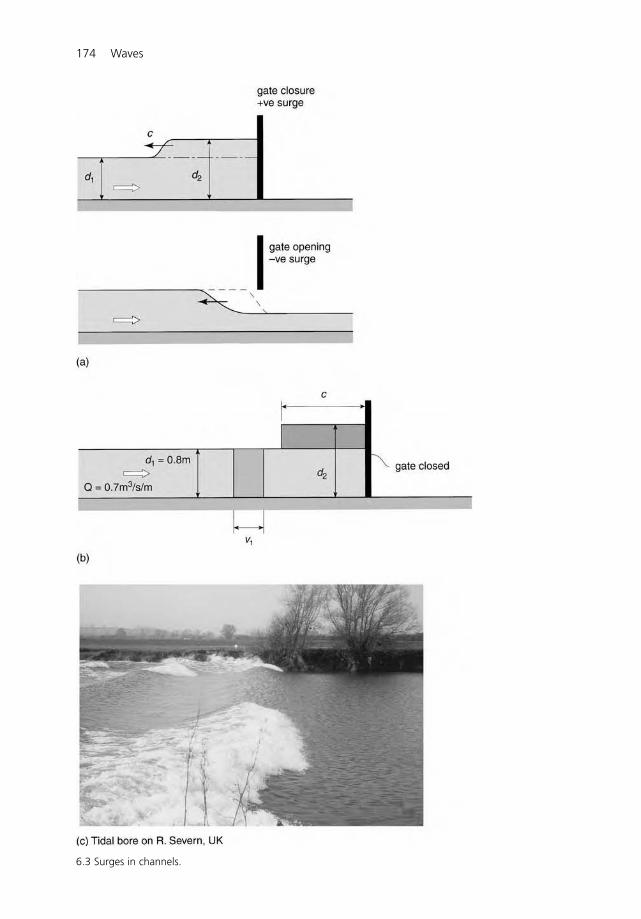
174 Waves
6.3 Surges in channels.
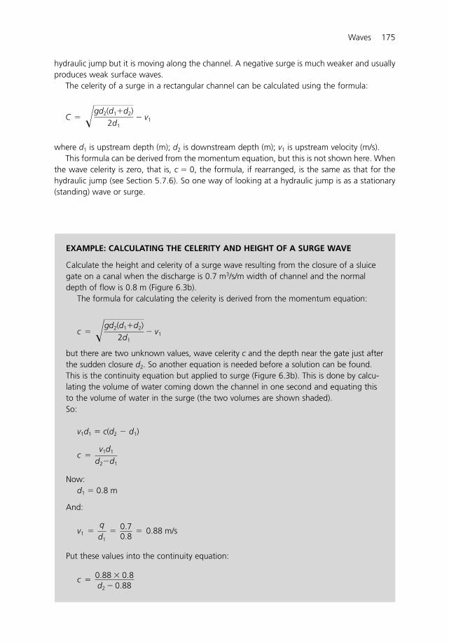
Waves 175
EXAMPLE: CALCULATING THE CELERITY AND HEIGHT OF A SURGE WAVE
Calculate the height and celerity of a surge wave resulting from the closure of a sluicegate on a canal when the discharge is 0.7 m3/s/m width of channel and the normaldepth of flow is 0.8 m (Figure 6.3b).
The formula for calculating the celerity is derived from the momentum equation:
but there are two unknown values, wave celerity c and the depth near the gate just afterthe sudden closure d2. So another equation is needed before a solution can be found.This is the continuity equation but applied to surge (Figure 6.3b). This is done by calcu-lating the volume of water coming down the channel in one second and equating thisto the volume of water in the surge (the two volumes are shown shaded).So:
v1d1 � c(d2 � d1)
Now:d1 � 0.8 m
And:
Put these values into the continuity equation:
c �
0.88 � 0.8d2 � 0.88
v1 �
qd1
�
0.70.8
� 0.88 m/s
c �
v1d1
d2�d1
c � �gd2(d1�d2)2d1
� v1
hydraulic jump but it is moving along the channel. A negative surge is much weaker and usuallyproduces weak surface waves.
The celerity of a surge in a rectangular channel can be calculated using the formula:
where d1 is upstream depth (m); d2 is downstream depth (m); v1 is upstream velocity (m/s).This formula can be derived from the momentum equation, but this is not shown here. When
the wave celerity is zero, that is, c � 0, the formula, if rearranged, is the same as that for thehydraulic jump (see Section 5.7.6). So one way of looking at a hydraulic jump is as a stationary(standing) wave or surge.
C � �gd2(d1�d2)2d1
� v1
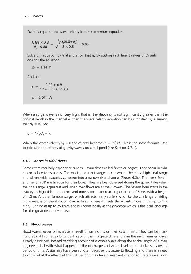
176 Waves
When a surge wave is not very high, that is, the depth d2 is not significantly greater than theoriginal depth in the channel d1 then the wave celerity equation can be simplified by assumingthat d1 � d2. So:
When the water velocity v1 � 0 the celerity becomes . This is the same formula usedto calculate the celerity of gravity waves on a still pond (see Section 5.7.1).
6.4.2 Bores in tidal rivers
Some rivers regularly experience surges – sometimes called bores or eagres. They occur in tidalreaches close to estuaries. The most prominent surges occur where there is a high tidal rangeand where wide estuaries converge into a narrow river channel (Figure 6.3c). The rivers Severnand Trent in UK are famous for their bores. They are best observed during the spring tides whenthe tidal range is greatest and when river flows are at their lowest. The Severn bore starts in theestuary as high tide approaches and moves upstream reaching celerities of 5 m/s with a heightof 1.5 m. Another famous surge, which attracts many surfers who like the challenge of ridingbig waves, is on the Amazon River in Brazil where it meets the Atlantic Ocean. It is up to 4 mhigh, running at up to 25 km/h and is known locally as the pororoca which is the local languagefor ‘the great destructive noise’.
6.5 Flood waves
Flood waves occur on rivers as a result of rainstorms on river catchments. They can be manyhundreds of kilometres long; dealing with them is quite different from the much smaller wavesalready described. Instead of taking account of a whole wave along the entire length of a river,engineers deal with what happens to the discharge and water levels at particular sites over aperiod of time. A site may have been chosen because it is prone to flooding and there is a needto know what the effects of this will be, or it may be a convenient site for accurately measuring
c � �gd
c � �gd1 � v1
Put this equal to the wave celerity in the momentum equation:
Solve this equation by trial and error, that is, by putting in different values of d2 untilone fits the equation:
d2 � 1.14 m
And so:
c � 2.07 m/s
c �
0.88 � 0.81.14 � 0.88 � 0.8
0.88 � 0.8d2�0.88
� �gd2(0.8�d2)2 � 0.8
� 0.88
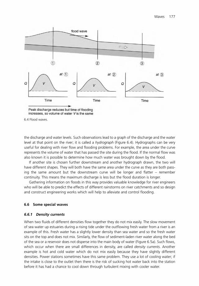
Waves 177
the discharge and water levels. Such observations lead to a graph of the discharge and the waterlevel at that point on the river; it is called a hydrograph (Figure 6.4). Hydrographs can be veryuseful for dealing with river flow and flooding problems. For example, the area under the curverepresents the volume of water that has passed the site during the flood. If the normal flow wasalso known it is possible to determine how much water was brought down by the flood.
If another site is chosen further downstream and another hydrograph drawn, the two willhave different shapes. They will both have the same area under the curve as they are both pass-ing the same amount but the downstream curve will be longer and flatter – remembercontinuity. This means the maximum discharge is less but the flood duration is longer.
Gathering information on floods in this way provides valuable knowledge for river engineerswho will be able to predict the effects of different rainstorms on river catchments and so designand construct engineering works which will help to alleviate and control flooding.
6.6 Some special waves
6.6.1 Density currents
When two fluids of different densities flow together they do not mix easily. The slow movementof sea water up estuaries during a rising tide under the outflowing fresh water from a river is anexample of this. Fresh water has a slightly lower density than sea water and so the fresh watersits on the top and does not mix. Similarly, the flow of sediment-laden river water along the bedof the sea or a reservoir does not disperse into the main body of water (Figure 6.5a). Such flows,which occur when there are small differences in density, are called density currents. Anotherexample is hot and cold water which do not mix easily because they have slightly differentdensities. Power stations sometimes have this same problem. They use a lot of cooling water; ifthe intake is close to the outlet then there is the risk of sucking hot water back into the stationbefore it has had a chance to cool down through turbulent mixing with cooler water.
6.4 Flood waves.
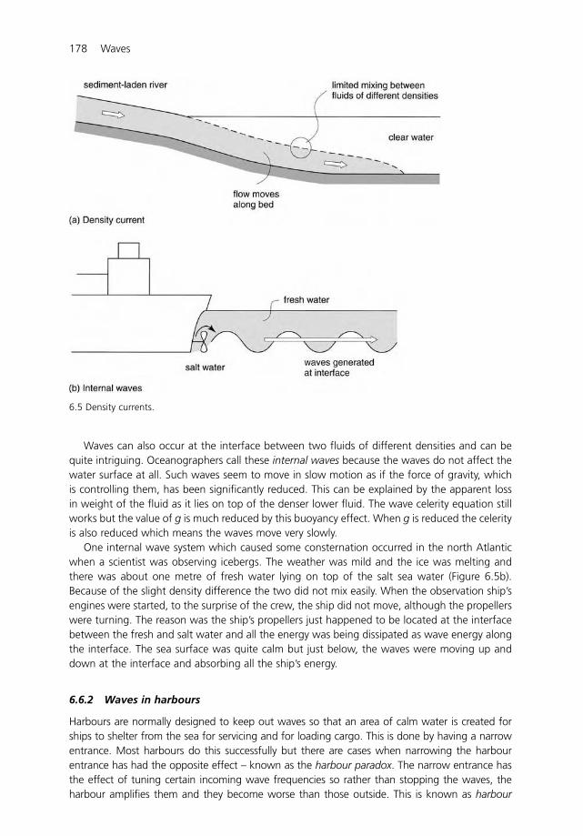
178 Waves
Waves can also occur at the interface between two fluids of different densities and can bequite intriguing. Oceanographers call these internal waves because the waves do not affect thewater surface at all. Such waves seem to move in slow motion as if the force of gravity, whichis controlling them, has been significantly reduced. This can be explained by the apparent lossin weight of the fluid as it lies on top of the denser lower fluid. The wave celerity equation stillworks but the value of g is much reduced by this buoyancy effect. When g is reduced the celerityis also reduced which means the waves move very slowly.
One internal wave system which caused some consternation occurred in the north Atlanticwhen a scientist was observing icebergs. The weather was mild and the ice was melting andthere was about one metre of fresh water lying on top of the salt sea water (Figure 6.5b).Because of the slight density difference the two did not mix easily. When the observation ship’sengines were started, to the surprise of the crew, the ship did not move, although the propellerswere turning. The reason was the ship’s propellers just happened to be located at the interfacebetween the fresh and salt water and all the energy was being dissipated as wave energy alongthe interface. The sea surface was quite calm but just below, the waves were moving up anddown at the interface and absorbing all the ship’s energy.
6.6.2 Waves in harbours
Harbours are normally designed to keep out waves so that an area of calm water is created forships to shelter from the sea for servicing and for loading cargo. This is done by having a narrowentrance. Most harbours do this successfully but there are cases when narrowing the harbourentrance has had the opposite effect – known as the harbour paradox. The narrow entrance hasthe effect of tuning certain incoming wave frequencies so rather than stopping the waves, theharbour amplifies them and they become worse than those outside. This is known as harbour
6.5 Density currents.
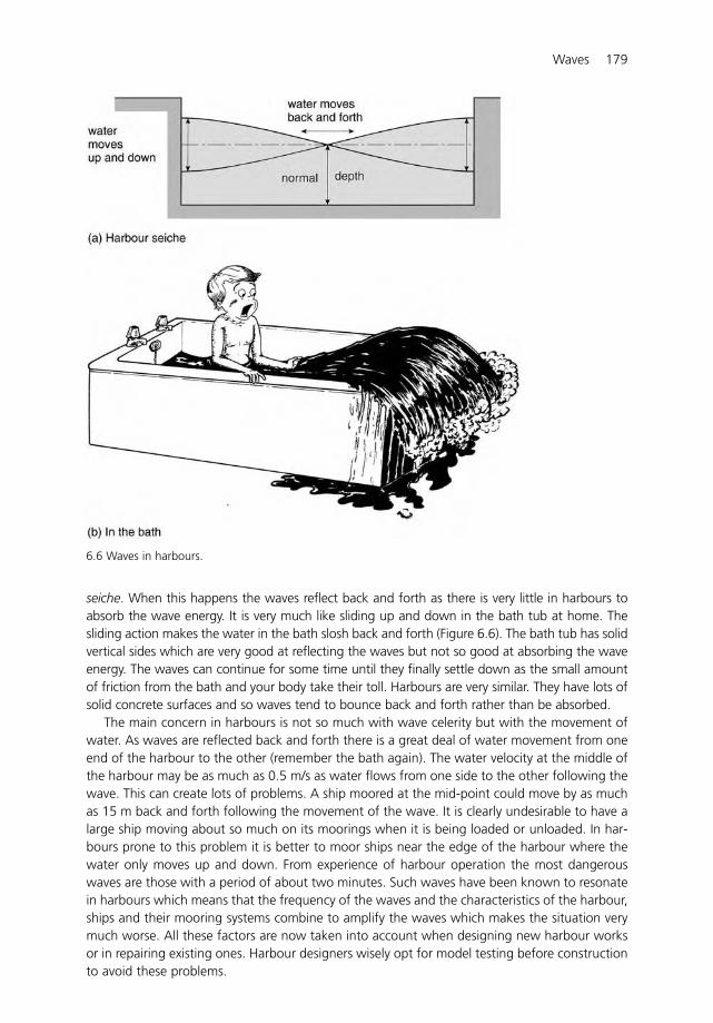
Waves 179
seiche. When this happens the waves reflect back and forth as there is very little in harbours toabsorb the wave energy. It is very much like sliding up and down in the bath tub at home. Thesliding action makes the water in the bath slosh back and forth (Figure 6.6). The bath tub has solidvertical sides which are very good at reflecting the waves but not so good at absorbing the waveenergy. The waves can continue for some time until they finally settle down as the small amountof friction from the bath and your body take their toll. Harbours are very similar. They have lots ofsolid concrete surfaces and so waves tend to bounce back and forth rather than be absorbed.
The main concern in harbours is not so much with wave celerity but with the movement ofwater. As waves are reflected back and forth there is a great deal of water movement from oneend of the harbour to the other (remember the bath again). The water velocity at the middle ofthe harbour may be as much as 0.5 m/s as water flows from one side to the other following thewave. This can create lots of problems. A ship moored at the mid-point could move by as muchas 15 m back and forth following the movement of the wave. It is clearly undesirable to have alarge ship moving about so much on its moorings when it is being loaded or unloaded. In har-bours prone to this problem it is better to moor ships near the edge of the harbour where thewater only moves up and down. From experience of harbour operation the most dangerouswaves are those with a period of about two minutes. Such waves have been known to resonatein harbours which means that the frequency of the waves and the characteristics of the harbour,ships and their mooring systems combine to amplify the waves which makes the situation verymuch worse. All these factors are now taken into account when designing new harbour worksor in repairing existing ones. Harbour designers wisely opt for model testing before constructionto avoid these problems.
6.6 Waves in harbours.

180 Waves
6.6.3 Tsunami wave
The tsunami is perhaps the most famous wave of all following the disastrous events in the IndianOcean on 26 December 2004 (Figure 6.7). The word tsunami is Japanese for a long wave causedby earthquakes or landslides under the ocean. There is a common misconception that tsunamisbehave like waves or swells which are generated by wind. They may have a similar appearancebut they have a very different origin. The sudden movement of the sea bed during an earth-quake causes a sudden movement of many millions of tons of water which can literally lift thesea level by a metre or more. The surge that comes from this weight of water has far greaterforce than any wind generated wave. This was evident from the devastating consequencesshown in the many photographs and videos taken of the 2004 event.
Tsunamis are most common in the Pacific ocean. They travel at very high celerity withdevastating consequences when they reach land. In the open ocean the wave may be only 0.5 mor so high but the wave celerity can be around 200 m/s when the ocean is say 5000 m deep.This might appear to be a surface wave but because of its great length its celerity is controlledby the depth of the ocean (remember the wave celerity equation ). Even so there is notmuch water displacement as it passes over the open ocean. A ship meeting this wave wouldhardly notice its passing. This is one of the reasons why many Indonesian fishermen survived the2005 tsunami. They were fishing in boats off the coast and hardly noticed the tsunami as itpassed underneath them. But nearer the shore was not a good place to be. As the tsunami runsinto shallow water, say 100 m deep, the wave slows down to 30 m/s but as the energy in thewave is still the same the wave height increases substantially. At 30 m/s this is still quite fast andwith the height increasing further as it runs up the beach it can do a great deal of damage toshore installations. The more destructive tsunamis are those which are funnelled into a narrowspace when the width of a beach or harbour is restricted in some way. This has the effect offunnelling the energy of the wave into the harbour with destructive consequences.
6.7 Tidal power
Waves can be very useful for generating power. The most promising method is to hold incomingand outgoing tides behind a dam (or barrage) and use the head to drive turbines to generate
c � �gd
6.7 A tsunami wave coming ashore in Thailand 2004.
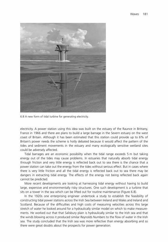
Waves 181
electricity. A power station using this idea was built on the estuary of the Raunce in Brittany,France in 1966 and there are plans to build a large barrage in the Severn estuary on the westcoast of Britain. Although it has been estimated that this station could provide up to 6% ofBritain’s power needs the scheme is hotly debated because it would affect the pattern of thetides and sediment movements in the estuary and many ecologically sensitive wetland sitescould be adversely affected.
Tidal barrages are an economic possibility when the tidal range exceeds 5 m but takingenergy out of the tides may cause problems. In estuaries that naturally absorb tidal energythrough friction and very little energy is reflected back out to sea there is the chance that apower station can take out the energy from the tides without serious effect. But in cases wherethere is very little friction and all the tidal energy is reflected back out to sea there may bedangers in extracting tidal energy. The effects of the energy not being reflected back againcannot be predicted.
More recent developments are looking at harnessing tidal energy without having to buildlarge, expensive and environmentally risky structures. One such development is a turbine thatsits on a tower in the sea which can be lifted out for routine maintenance (Figure 6.8).
In the 1920s one enterprising engineer undertook a study to establish the feasibility ofconstructing tidal power stations across the Irish Sea between Ireland and Wales and Ireland andScotland. Because of the difficulties and high costs of measuring velocities across this largestretch of water he looked around for a hydraulically similar model on which to make measure-ments. He worked out that that Salisbury plain is hydraulically similar to the Irish sea and thatthe winds blowing across it produced similar Reynolds Numbers to the flow of water in the Irishsea. The study concluded that the Irish sea was more reflective than energy absorbing and sothere were great doubts about the prospects for power generation.
6.8 A new form of tidal turbine for generating electricity.
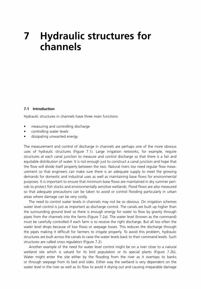
7 Hydraulic structures forchannels
7.1 Introduction
Hydraulic structures in channels have three main functions:
• measuring and controlling discharge• controlling water levels• dissipating unwanted energy.
The measurement and control of discharge in channels are perhaps one of the more obvioususes of hydraulic structures (Figure 7.1). Large irrigation networks, for example, requirestructures at each canal junction to measure and control discharge so that there is a fair andequitable distribution of water. It is not enough just to construct a canal junction and hope thatthe flow will divide itself properly between the two. Natural rivers too need regular flow meas-urement so that engineers can make sure there is an adequate supply to meet the growingdemands for domestic and industrial uses as well as maintaining base flows for environmentalpurposes. It is important to ensure that minimum base flows are maintained in dry summer peri-ods to protect fish stocks and environmentally sensitive wetlands. Flood flows are also measuredso that adequate precautions can be taken to avoid or control flooding particularly in urbanareas where damage can be very costly.
The need to control water levels in channels may not be so obvious. On irrigation schemeswater level control is just as important as discharge control. The canals are built up higher thanthe surrounding ground level so there is enough energy for water to flow by gravity throughpipes from the channels into the farms (Figure 7.2a). The water level (known as the command)must be carefully controlled if each farm is to receive the right discharge. But all too often thewater level drops because of low flows or seepage losses. This reduces the discharge throughthe pipes making it difficult for farmers to irrigate properly. To avoid this problem, hydraulicstructures are built across the canals to raise the water levels back to their command levels. Suchstructures are called cross regulators (Figure 7.2).
Another example of the need for water level control might be on a river close to a naturalwetland site which is valued for its bird population or its special plants (Figure 7.2b).Water might enter the site either by the flooding from the river as it overtops its banksor through seepage from its bed and sides. Either way the wetland is very dependent on thewater level in the river as well as its flow to avoid it drying out and causing irreparable damage
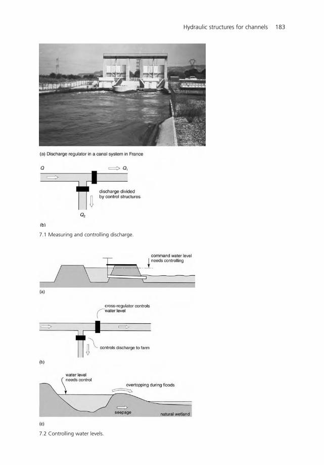
Hydraulic structures for channels 183
7.1 Measuring and controlling discharge.
7.2 Controlling water levels.
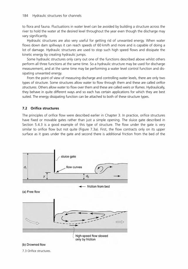
184 Hydraulic structures for channels
to flora and fauna. Fluctuations in water level can be avoided by building a structure across theriver to hold the water at the desired level throughout the year even though the discharge mayvary significantly.
Hydraulic structures are also very useful for getting rid of unwanted energy. When waterflows down dam spillways it can reach speeds of 60 km/h and more and is capable of doing alot of damage. Hydraulic structures are used to stop such high speed flows and dissipate thekinetic energy by creating hydraulic jumps.
Some hydraulic structures only carry out one of the functions described above whilst othersperform all three functions at the same time. So a hydraulic structure may be used for dischargemeasurement, and at the same time may be performing a water level control function and dis-sipating unwanted energy.
From the point of view of measuring discharge and controlling water levels, there are only twotypes of structure. Some structures allow water to flow through them and these are called orificestructures. Others allow water to flow over them and these are called weirs or flumes. Hydraulically,they behave in quite different ways and so each has certain applications for which they are bestsuited. The energy dissipating function can be attached to both of these structure types.
7.2 Orifice structures
The principles of orifice flow were described earlier in Chapter 3. In practice, orifice structureshave fixed or movable gates rather than just a simple opening. The sluice gate described inSection 5.4.3 is a good example of this type of structure. The flow under the gate is verysimilar to orifice flow but not quite (Figure 7.3a). First, the flow contracts only on its uppersurface as it goes under the gate and second there is additional friction from the bed of the
7.3 Orifice structures.
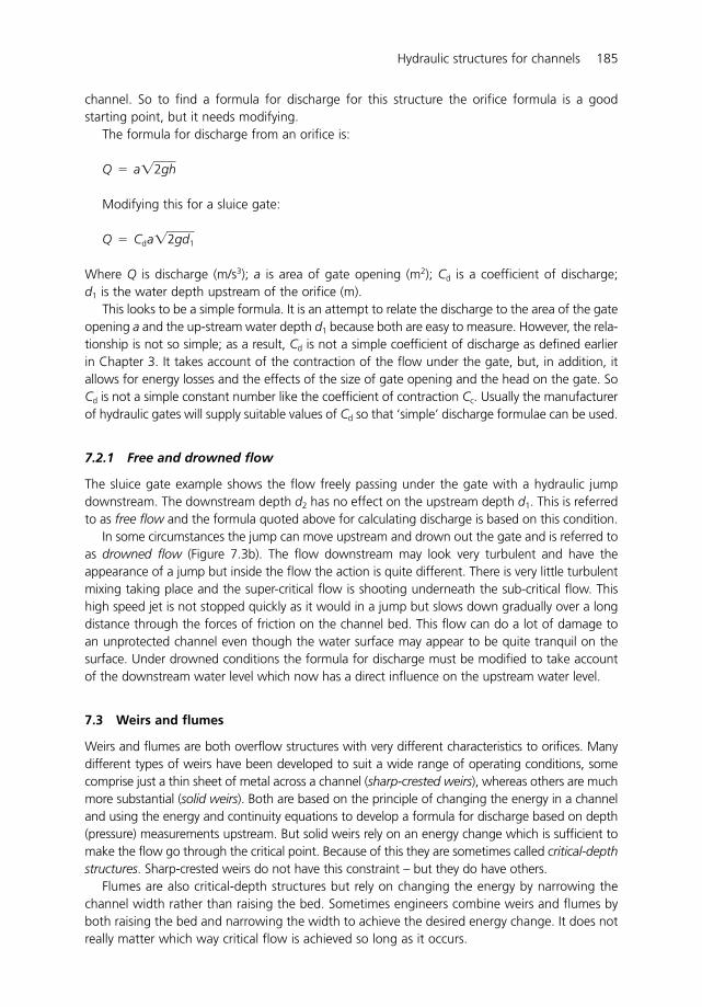
Hydraulic structures for channels 185
channel. So to find a formula for discharge for this structure the orifice formula is a goodstarting point, but it needs modifying.
The formula for discharge from an orifice is:
Modifying this for a sluice gate:
Where Q is discharge (m/s3); a is area of gate opening (m2); Cd is a coefficient of discharge; d1 is the water depth upstream of the orifice (m).
This looks to be a simple formula. It is an attempt to relate the discharge to the area of the gateopening a and the up-stream water depth d1 because both are easy to measure. However, the rela-tionship is not so simple; as a result, Cd is not a simple coefficient of discharge as defined earlierin Chapter 3. It takes account of the contraction of the flow under the gate, but, in addition, itallows for energy losses and the effects of the size of gate opening and the head on the gate. SoCd is not a simple constant number like the coefficient of contraction Cc. Usually the manufacturerof hydraulic gates will supply suitable values of Cd so that ‘simple’ discharge formulae can be used.
7.2.1 Free and drowned flow
The sluice gate example shows the flow freely passing under the gate with a hydraulic jumpdownstream. The downstream depth d2 has no effect on the upstream depth d1. This is referredto as free flow and the formula quoted above for calculating discharge is based on this condition.
In some circumstances the jump can move upstream and drown out the gate and is referred toas drowned flow (Figure 7.3b). The flow downstream may look very turbulent and have theappearance of a jump but inside the flow the action is quite different. There is very little turbulentmixing taking place and the super-critical flow is shooting underneath the sub-critical flow. Thishigh speed jet is not stopped quickly as it would in a jump but slows down gradually over a longdistance through the forces of friction on the channel bed. This flow can do a lot of damage toan unprotected channel even though the water surface may appear to be quite tranquil on thesurface. Under drowned conditions the formula for discharge must be modified to take accountof the downstream water level which now has a direct influence on the upstream water level.
7.3 Weirs and flumes
Weirs and flumes are both overflow structures with very different characteristics to orifices. Manydifferent types of weirs have been developed to suit a wide range of operating conditions, somecomprise just a thin sheet of metal across a channel (sharp-crested weirs), whereas others are muchmore substantial (solid weirs). Both are based on the principle of changing the energy in a channeland using the energy and continuity equations to develop a formula for discharge based on depth(pressure) measurements upstream. But solid weirs rely on an energy change which is sufficient tomake the flow go through the critical point. Because of this they are sometimes called critical-depthstructures. Sharp-crested weirs do not have this constraint – but they do have others.
Flumes are also critical-depth structures but rely on changing the energy by narrowing thechannel width rather than raising the bed. Sometimes engineers combine weirs and flumes byboth raising the bed and narrowing the width to achieve the desired energy change. It does notreally matter which way critical flow is achieved so long as it occurs.
Q � Cda�2gd1
Q � a�2gh
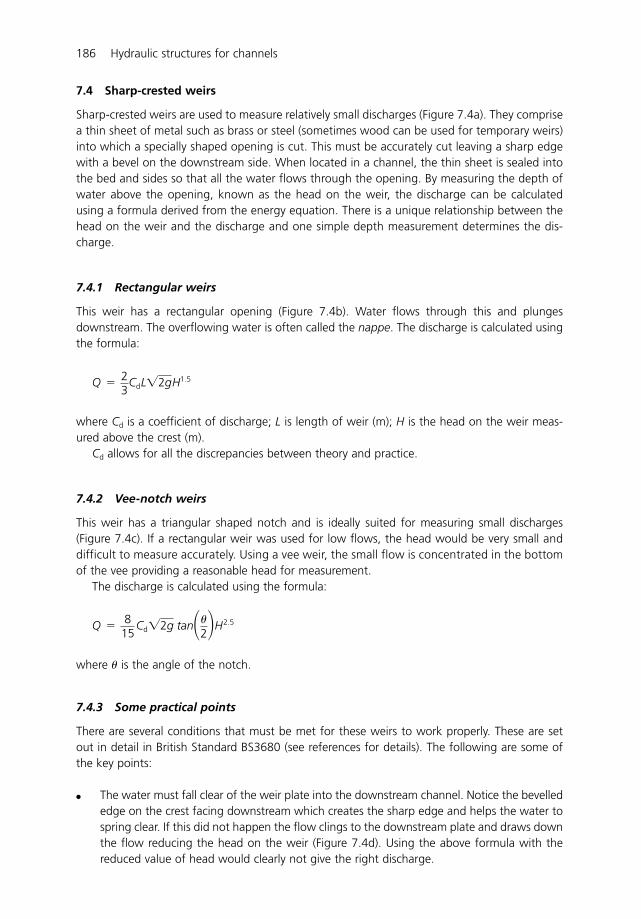
186 Hydraulic structures for channels
7.4 Sharp-crested weirs
Sharp-crested weirs are used to measure relatively small discharges (Figure 7.4a). They comprisea thin sheet of metal such as brass or steel (sometimes wood can be used for temporary weirs)into which a specially shaped opening is cut. This must be accurately cut leaving a sharp edgewith a bevel on the downstream side. When located in a channel, the thin sheet is sealed intothe bed and sides so that all the water flows through the opening. By measuring the depth ofwater above the opening, known as the head on the weir, the discharge can be calculatedusing a formula derived from the energy equation. There is a unique relationship between thehead on the weir and the discharge and one simple depth measurement determines the dis-charge.
7.4.1 Rectangular weirs
This weir has a rectangular opening (Figure 7.4b). Water flows through this and plungesdownstream. The overflowing water is often called the nappe. The discharge is calculated usingthe formula:
where Cd is a coefficient of discharge; L is length of weir (m); H is the head on the weir meas-ured above the crest (m).
Cd allows for all the discrepancies between theory and practice.
7.4.2 Vee-notch weirs
This weir has a triangular shaped notch and is ideally suited for measuring small discharges(Figure 7.4c). If a rectangular weir was used for low flows, the head would be very small anddifficult to measure accurately. Using a vee weir, the small flow is concentrated in the bottomof the vee providing a reasonable head for measurement.
The discharge is calculated using the formula:
where is the angle of the notch.
7.4.3 Some practical points
There are several conditions that must be met for these weirs to work properly. These are setout in detail in British Standard BS3680 (see references for details). The following are some ofthe key points:
� The water must fall clear of the weir plate into the downstream channel. Notice the bevellededge on the crest facing downstream which creates the sharp edge and helps the water tospring clear. If this did not happen the flow clings to the downstream plate and draws downthe flow reducing the head on the weir (Figure 7.4d). Using the above formula with thereduced value of head would clearly not give the right discharge.
Q �
815
Cd�2g tan�2�H2.5
Q �
23
CdL�2gH1.5
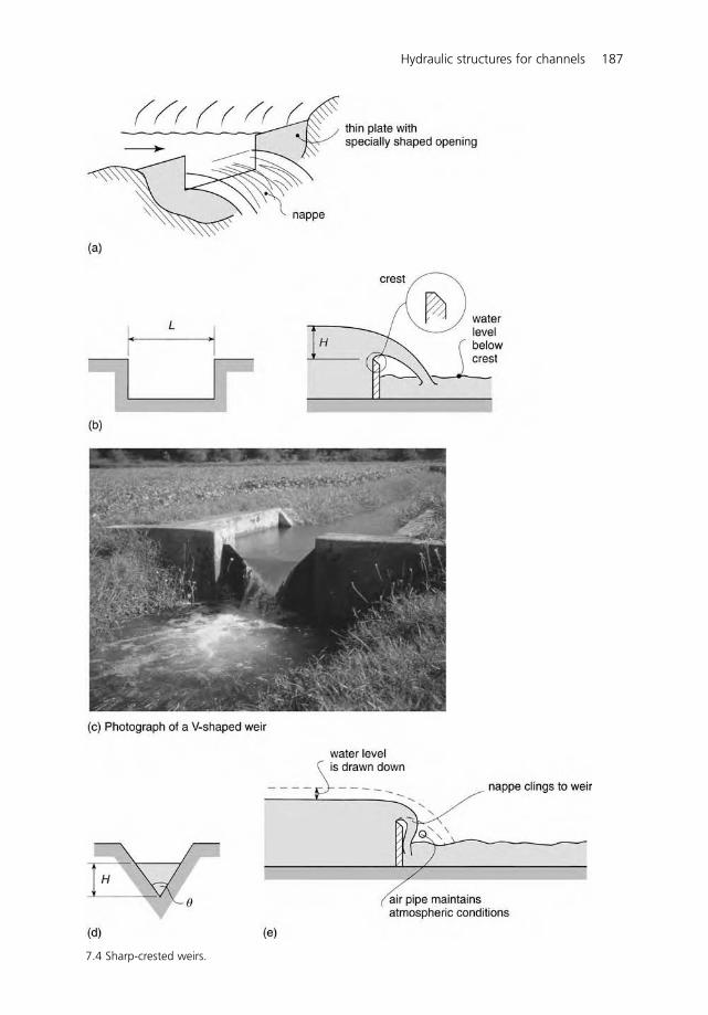
Hydraulic structures for channels 187
7.4 Sharp-crested weirs.
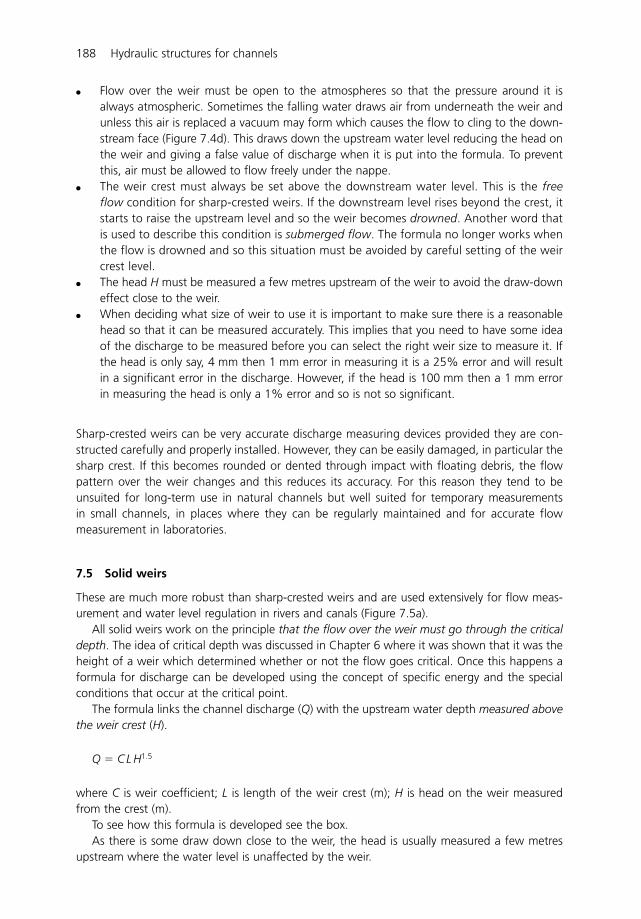
188 Hydraulic structures for channels
� Flow over the weir must be open to the atmospheres so that the pressure around it isalways atmospheric. Sometimes the falling water draws air from underneath the weir andunless this air is replaced a vacuum may form which causes the flow to cling to the down-stream face (Figure 7.4d). This draws down the upstream water level reducing the head onthe weir and giving a false value of discharge when it is put into the formula. To preventthis, air must be allowed to flow freely under the nappe.
� The weir crest must always be set above the downstream water level. This is the freeflow condition for sharp-crested weirs. If the downstream level rises beyond the crest, itstarts to raise the upstream level and so the weir becomes drowned. Another word thatis used to describe this condition is submerged flow. The formula no longer works whenthe flow is drowned and so this situation must be avoided by careful setting of the weircrest level.
� The head H must be measured a few metres upstream of the weir to avoid the draw-downeffect close to the weir.
� When deciding what size of weir to use it is important to make sure there is a reasonablehead so that it can be measured accurately. This implies that you need to have some ideaof the discharge to be measured before you can select the right weir size to measure it. Ifthe head is only say, 4 mm then 1 mm error in measuring it is a 25% error and will resultin a significant error in the discharge. However, if the head is 100 mm then a 1 mm errorin measuring the head is only a 1% error and so is not so significant.
Sharp-crested weirs can be very accurate discharge measuring devices provided they are con-structed carefully and properly installed. However, they can be easily damaged, in particular thesharp crest. If this becomes rounded or dented through impact with floating debris, the flowpattern over the weir changes and this reduces its accuracy. For this reason they tend to beunsuited for long-term use in natural channels but well suited for temporary measurementsin small channels, in places where they can be regularly maintained and for accurate flowmeasurement in laboratories.
7.5 Solid weirs
These are much more robust than sharp-crested weirs and are used extensively for flow meas-urement and water level regulation in rivers and canals (Figure 7.5a).
All solid weirs work on the principle that the flow over the weir must go through the criticaldepth. The idea of critical depth was discussed in Chapter 6 where it was shown that it was theheight of a weir which determined whether or not the flow goes critical. Once this happens aformula for discharge can be developed using the concept of specific energy and the specialconditions that occur at the critical point.
The formula links the channel discharge (Q) with the upstream water depth measured abovethe weir crest (H).
Q � C L H1.5
where C is weir coefficient; L is length of the weir crest (m); H is head on the weir measuredfrom the crest (m).
To see how this formula is developed see the box.As there is some draw down close to the weir, the head is usually measured a few metres
upstream where the water level is unaffected by the weir.
Hydraulic structures for channels 189
DERIVATION: FORMULA FOR DISCHARGE OVER A CRITICAL FLOW STRUCTURE
Derive a formula for discharge for a critical flow structure in an open channel. Use abroad-crested weir as an example of a critical flow structure, although the analysis wouldbe the same for any similar structure (Figure 7.5b).
First write down the total energy equation for the flow in the channel (point 1) and theflow on the weir (point 2):
total energy at point 1 � total energy at point 2
Now:
That is, the height of the weir is equal to the difference in the potential energy and so:
But at the critical depth:
d2 � dc
And:
v2 � vc
d1 �
v21
2g � d2 �
v22
2g � y
z2 � z1 � y
d1 �
v21
2g � z1 � d2 �
v22
2g � z2
7.5 Solid weirs.
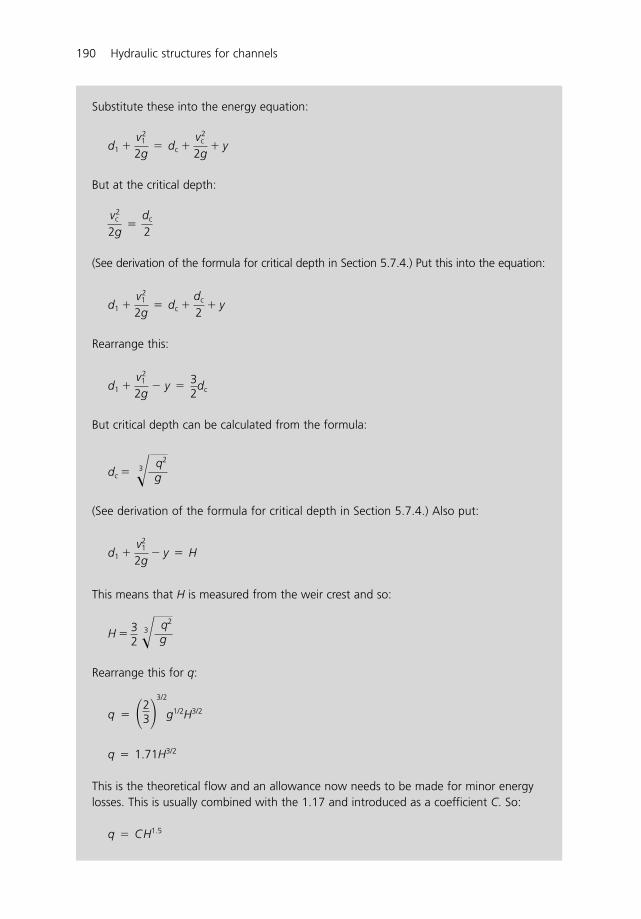
190 Hydraulic structures for channels
Substitute these into the energy equation:
But at the critical depth:
(See derivation of the formula for critical depth in Section 5.7.4.) Put this into the equation:
Rearrange this:
But critical depth can be calculated from the formula:
(See derivation of the formula for critical depth in Section 5.7.4.) Also put:
This means that H is measured from the weir crest and so:
Rearrange this for q:
This is the theoretical flow and an allowance now needs to be made for minor energylosses. This is usually combined with the 1.17 and introduced as a coefficient C. So:
q � CH1.5
q � 1.71H3/2
q � �23�
3/2
g1/2H3/2
H �32
3� q2
g
d1 �
v21
2g � y � H
dc �
3� q2
g
d1 �
v21
2g � y �
32
dc
d1 �
v21
2g � dc �
dc
2 � y
v2c
2g �
dc
2
d1 �
v21
2g � dc �
v2c
2g � y
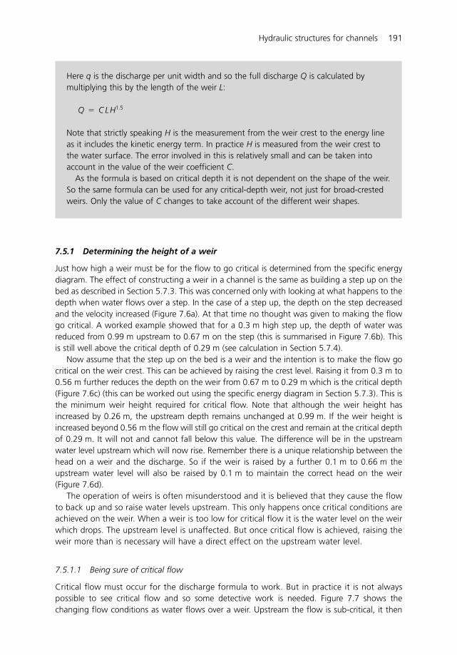
Hydraulic structures for channels 191
7.5.1 Determining the height of a weir
Just how high a weir must be for the flow to go critical is determined from the specific energydiagram. The effect of constructing a weir in a channel is the same as building a step up on thebed as described in Section 5.7.3. This was concerned only with looking at what happens to thedepth when water flows over a step. In the case of a step up, the depth on the step decreasedand the velocity increased (Figure 7.6a). At that time no thought was given to making the flowgo critical. A worked example showed that for a 0.3 m high step up, the depth of water wasreduced from 0.99 m upstream to 0.67 m on the step (this is summarised in Figure 7.6b). Thisis still well above the critical depth of 0.29 m (see calculation in Section 5.7.4).
Now assume that the step up on the bed is a weir and the intention is to make the flow gocritical on the weir crest. This can be achieved by raising the crest level. Raising it from 0.3 m to0.56 m further reduces the depth on the weir from 0.67 m to 0.29 m which is the critical depth(Figure 7.6c) (this can be worked out using the specific energy diagram in Section 5.7.3). This isthe minimum weir height required for critical flow. Note that although the weir height hasincreased by 0.26 m, the upstream depth remains unchanged at 0.99 m. If the weir height isincreased beyond 0.56 m the flow will still go critical on the crest and remain at the critical depthof 0.29 m. It will not and cannot fall below this value. The difference will be in the upstreamwater level upstream which will now rise. Remember there is a unique relationship between thehead on a weir and the discharge. So if the weir is raised by a further 0.1 m to 0.66 m theupstream water level will also be raised by 0.1 m to maintain the correct head on the weir(Figure 7.6d).
The operation of weirs is often misunderstood and it is believed that they cause the flowto back up and so raise water levels upstream. This only happens once critical conditions areachieved on the weir. When a weir is too low for critical flow it is the water level on the weirwhich drops. The upstream level is unaffected. But once critical flow is achieved, raising theweir more than is necessary will have a direct effect on the upstream water level.
7.5.1.1 Being sure of critical flow
Critical flow must occur for the discharge formula to work. But in practice it is not alwayspossible to see critical flow and so some detective work is needed. Figure 7.7 shows thechanging flow conditions as water flows over a weir. Upstream the flow is sub-critical, it then
Here q is the discharge per unit width and so the full discharge Q is calculated bymultiplying this by the length of the weir L:
Note that strictly speaking H is the measurement from the weir crest to the energy lineas it includes the kinetic energy term. In practice H is measured from the weir crest tothe water surface. The error involved in this is relatively small and can be taken intoaccount in the value of the weir coefficient C.
As the formula is based on critical depth it is not dependent on the shape of the weir.So the same formula can be used for any critical-depth weir, not just for broad-crestedweirs. Only the value of C changes to take account of the different weir shapes.
Q � C LH1.5
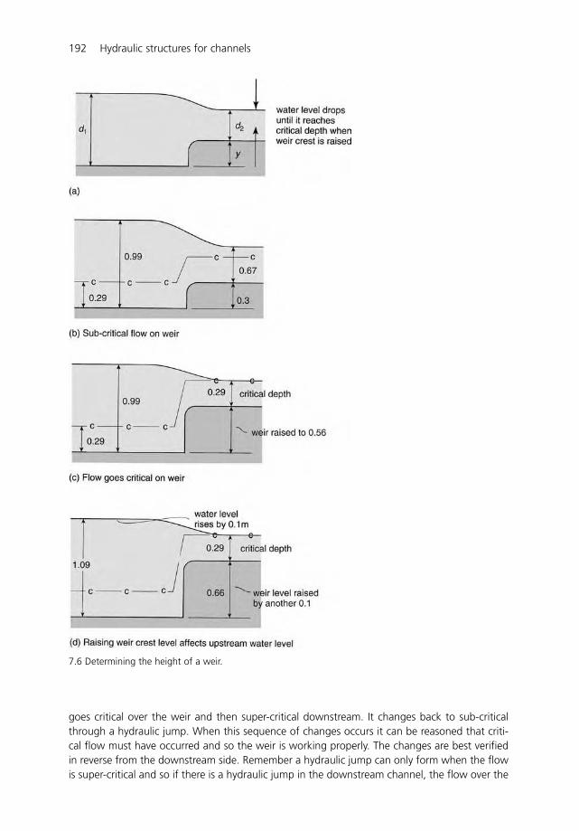
192 Hydraulic structures for channels
7.6 Determining the height of a weir.
goes critical over the weir and then super-critical downstream. It changes back to sub-criticalthrough a hydraulic jump. When this sequence of changes occurs it can be reasoned that criti-cal flow must have occurred and so the weir is working properly. The changes are best verifiedin reverse from the downstream side. Remember a hydraulic jump can only form when the flowis super-critical and so if there is a hydraulic jump in the downstream channel, the flow over the
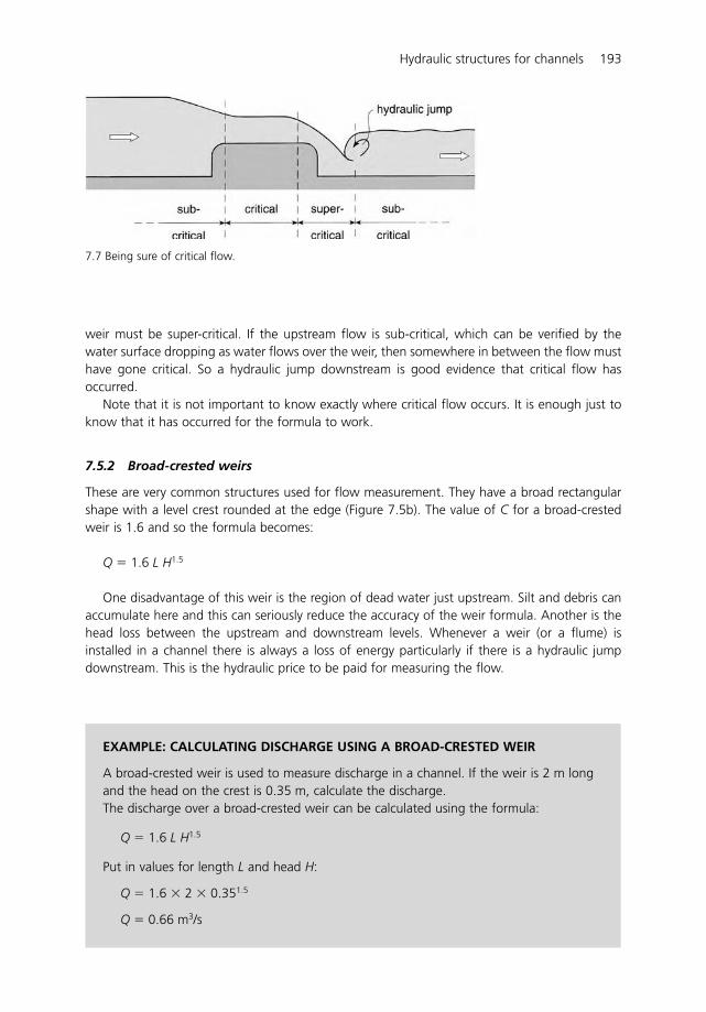
Hydraulic structures for channels 193
EXAMPLE: CALCULATING DISCHARGE USING A BROAD-CRESTED WEIR
A broad-crested weir is used to measure discharge in a channel. If the weir is 2 m longand the head on the crest is 0.35 m, calculate the discharge.The discharge over a broad-crested weir can be calculated using the formula:
Q � 1.6 L H1.5
Put in values for length L and head H:
Q � 1.6 � 2 � 0.351.5
Q � 0.66 m3/s
weir must be super-critical. If the upstream flow is sub-critical, which can be verified by thewater surface dropping as water flows over the weir, then somewhere in between the flow musthave gone critical. So a hydraulic jump downstream is good evidence that critical flow hasoccurred.
Note that it is not important to know exactly where critical flow occurs. It is enough just toknow that it has occurred for the formula to work.
7.5.2 Broad-crested weirs
These are very common structures used for flow measurement. They have a broad rectangularshape with a level crest rounded at the edge (Figure 7.5b). The value of C for a broad-crestedweir is 1.6 and so the formula becomes:
Q � 1.6 L H1.5
One disadvantage of this weir is the region of dead water just upstream. Silt and debris canaccumulate here and this can seriously reduce the accuracy of the weir formula. Another is thehead loss between the upstream and downstream levels. Whenever a weir (or a flume) isinstalled in a channel there is always a loss of energy particularly if there is a hydraulic jumpdownstream. This is the hydraulic price to be paid for measuring the flow.
7.7 Being sure of critical flow.
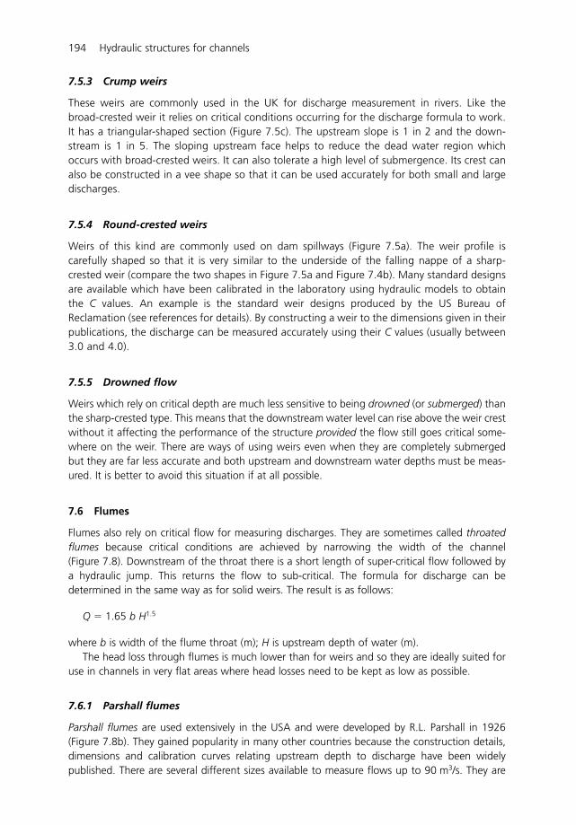
194 Hydraulic structures for channels
7.5.3 Crump weirs
These weirs are commonly used in the UK for discharge measurement in rivers. Like the broad-crested weir it relies on critical conditions occurring for the discharge formula to work.It has a triangular-shaped section (Figure 7.5c). The upstream slope is 1 in 2 and the down-stream is 1 in 5. The sloping upstream face helps to reduce the dead water region whichoccurs with broad-crested weirs. It can also tolerate a high level of submergence. Its crest canalso be constructed in a vee shape so that it can be used accurately for both small and largedischarges.
7.5.4 Round-crested weirs
Weirs of this kind are commonly used on dam spillways (Figure 7.5a). The weir profile iscarefully shaped so that it is very similar to the underside of the falling nappe of a sharp-crested weir (compare the two shapes in Figure 7.5a and Figure 7.4b). Many standard designsare available which have been calibrated in the laboratory using hydraulic models to obtainthe C values. An example is the standard weir designs produced by the US Bureau ofReclamation (see references for details). By constructing a weir to the dimensions given in theirpublications, the discharge can be measured accurately using their C values (usually between3.0 and 4.0).
7.5.5 Drowned flow
Weirs which rely on critical depth are much less sensitive to being drowned (or submerged) thanthe sharp-crested type. This means that the downstream water level can rise above the weir crestwithout it affecting the performance of the structure provided the flow still goes critical some-where on the weir. There are ways of using weirs even when they are completely submergedbut they are far less accurate and both upstream and downstream water depths must be meas-ured. It is better to avoid this situation if at all possible.
7.6 Flumes
Flumes also rely on critical flow for measuring discharges. They are sometimes called throatedflumes because critical conditions are achieved by narrowing the width of the channel(Figure 7.8). Downstream of the throat there is a short length of super-critical flow followed bya hydraulic jump. This returns the flow to sub-critical. The formula for discharge can bedetermined in the same way as for solid weirs. The result is as follows:
Q � 1.65 b H1.5
where b is width of the flume throat (m); H is upstream depth of water (m).The head loss through flumes is much lower than for weirs and so they are ideally suited for
use in channels in very flat areas where head losses need to be kept as low as possible.
7.6.1 Parshall flumes
Parshall flumes are used extensively in the USA and were developed by R.L. Parshall in 1926(Figure 7.8b). They gained popularity in many other countries because the construction details,dimensions and calibration curves relating upstream depth to discharge have been widelypublished. There are several different sizes available to measure flows up to 90 m3/s. They are
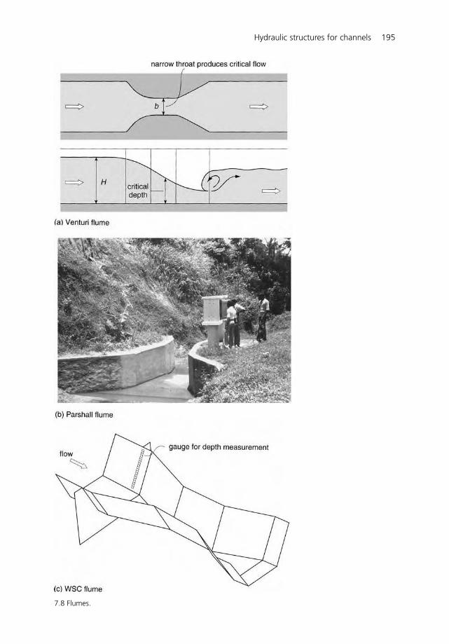
Hydraulic structures for channels 195
7.8 Flumes.
196 Hydraulic structures for channels
relatively simple to construct from a range of materials such as wood, concrete and metalbecause they have no curved surfaces.
If they are made and installed as recommended they provide accurate discharge measurement.
7.6.2 WSC flumes
This is a range of standard flumes for measuring small discharges from less than 1.0 l/s up to50 l/s developed by Washington State University in USA (Figure 7.8c). They are vee-shaped sothat they can be used to measure low flows accurately and, like Parshall flumes, they can beeasily made up in a workshop from metal or glass fibre. They are particularly useful as portableflumes for spot measurements in small channels and irrigation furrows.
7.6.3 Combination weir-flumes
Sometimes both weir and flume effects are combined to achieve critical flow. The advantagesof the vee for low flows can also be added. In such cases a laboratory model test is needed todetermine the C value in the discharge equation.
7.7 Discharge measurement
Weirs, flumes and orifices can all be used for discharge measurement. But weirs and flumes arebetter suited to measuring discharges in rivers when there can be large variations in flow. Weirsand flumes not only require a simple head reading to measure discharge but they can also passlarge flows without causing the upstream level to rise significantly and cause flooding. Orificestructures too can be used for flow measurement but both upstream and downstream waterlevels are usually required to determine discharge. Large variations in flow also mean that thegates will need constant attention for opening and closing.
7.8 Discharge control
Although orifices are rather cumbersome for discharge measurement they are very useful fordischarge control. This is because the discharge through an orifice is not very sensitive tochanges in upstream water level. Consider as an example, an irrigation canal system where abranch canal takes water from a main canal (Figure 7.9a). The structure at the head of thebranch controls the discharge to farmers downstream. The ideal structure for this would be anorifice and the reason lies in its hydraulic characteristic curve (Figure 7.9b). This is a graph of theorifice discharge equation:
In this simple example, the orifice opening is assumed to be fixed and so discharge Q changesonly when the upstream depth d1 changes. The point Qd and dd on the graph represents thenormal operating condition. Now suppose the main canal operating depth rises by say, 20%,because of changes in the water demand elsewhere in the system. The effect that this wouldhave on the discharge into the branch (through the orifice) is to change it by only 5%. So eventhough there is a significant change in the main canal this is hardly noticed in the branch. Thiscan be very useful for ensuring a reliable, constant flow to a farmer even though the main canalmay be varying considerably due to changing demands.
Q � C �2gd1
Hydraulic structures for channels 197
7.9 Discharge control.
In contrast, if a weir (or flume) is installed at the head of the branch canal, it would be veryeasy to use for discharge measurement but it would not be so good for controlling the flow.Again look at the hydraulic characteristic curve for a weir (Figure 7.9). This is a graph of the weirdischarge equation:
Q � C L H1.5
Qd and Hd represent the normal operating condition. Now if the water level in the maincanal rises by 20% this almost doubles the discharge in the branch canal. So this type ofstructure is very sensitive to water level changes and would not make a very good dischargecontrol structure.

198 Hydraulic structures for channels
These examples show the sensitivity of the two types of control structure. This is how theyreact to small changes in water level. But they refer to fixed structures. Most structures havegates (both weirs and orifices) which can be used to adjust the discharge but this adds to theburden of managing the channels. Better to use a structure which is hydraulically suited to thejob to be done and which reduces the need for continual monitoring and adjustment.
7.9 Water level control
Orifices, weirs and flumes can all be used for water level control. But the very reason thatmakes an orifice a good discharge regulator make it unsuitable for good water level control.Conversely, a weir (or flume) is well suited to water level control but not for discharge control.
Imagine the water level in a river needs to be controlled to stabilise water levels in a nearbywetland site and it needs to be more or less the same both winter and summer even thoughthe river flows change from a small flow to a flood. The structure best suited for this would bea weir as it can pass a wide range of flows with only small changes in head (water level). Anorifice structure would not be suitable because large changes in water level would occur as theflow changed and the structure would require a great deal of attention and adjustment.
Another water level control problem occurs in reservoirs. When a dam is built across a riverto store water, a spillway is also constructed to pass severe flood flows safely into the down-stream channel to avoid over-topping the dam. The ideal structure for this is a weir becauselarge discharges can flow over it for relatively small increases in water level. The rise in waterlevel can be calculated using the weir discharge formula and this helps to determine the heightof the dam. A freeboard is also added to the anticipated maximum water level as an addedsafety measure. The spillway can be the most expensive part of constructing a new dam. Manysmall dams are built on small seasonal streams in developing countries to conserve water fordomestic and agricultural use. But even a small dam will need a spillway and although thestream may look small and dry up occasionally, they can suffer from very severe floods whichare difficult to determine in advance, particularly when rainfall and discharge data for thestream are not available. Building a spillway for such conditions can be prohibitively expensiveand far exceed the cost of the dam and so it may be cheaper in sparsely populated areas to letthe dam be washed away and then re-build it on the rare occasions that this happens. Thereare of course many other factors to take into account besides dam reconstruction costs, suchas the effects downstream of a dam break. It is a sobering thought that even the biggest andmost important dams can fail because of severe flooding. They have large spillways to protectthem from very severe floods which are carefully assessed at the design stage. But it is impos-sible to say that they will safely carry every flood. Nature seems to have a way of testing us bysending unexpected rainstorms but fortunately these events are few and far between.
One way of avoiding the expensive spillway problem is to construct a reservoir at the side ofa river rather than use the river channel itself. This is called off-stream storage. Water is takenfrom the river by gravity or by pumping into a reservoir and only a modest spillway is thenneeded which would have the same capacity as the inlet discharge. When a flood comes downthe river there is no obstruction in its path and so it flows safely pass the reservoir.
7.10 Energy dissipators
7.10.1 Stilling basins
When water flows over a weir or through a flume and becomes super-critical it can do a lot ofdamage to the downstream channel if it is left unprotected. This is particularly true when water rushes
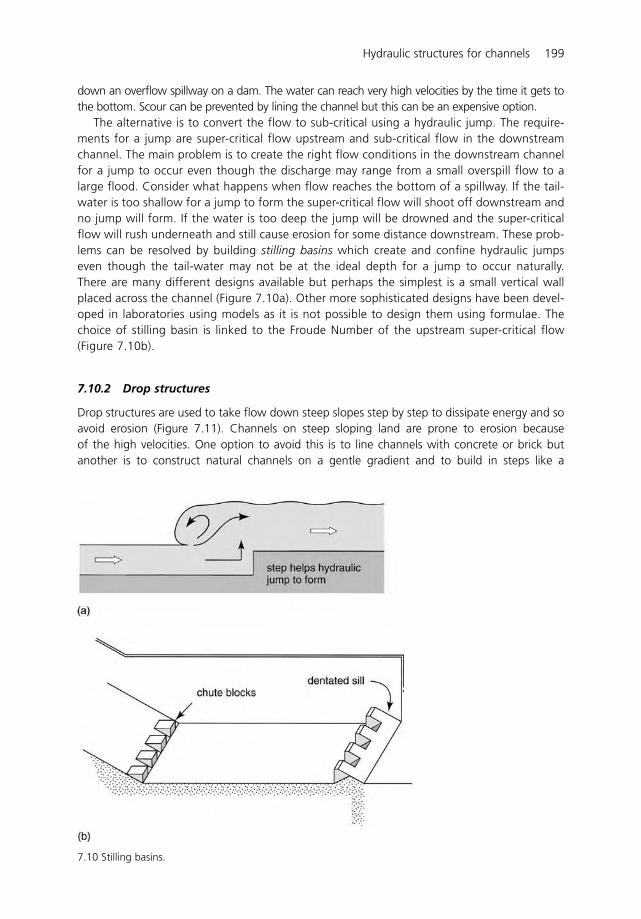
Hydraulic structures for channels 199
7.10 Stilling basins.
down an overflow spillway on a dam. The water can reach very high velocities by the time it gets tothe bottom. Scour can be prevented by lining the channel but this can be an expensive option.
The alternative is to convert the flow to sub-critical using a hydraulic jump. The require-ments for a jump are super-critical flow upstream and sub-critical flow in the downstreamchannel. The main problem is to create the right flow conditions in the downstream channelfor a jump to occur even though the discharge may range from a small overspill flow to alarge flood. Consider what happens when flow reaches the bottom of a spillway. If the tail-water is too shallow for a jump to form the super-critical flow will shoot off downstream andno jump will form. If the water is too deep the jump will be drowned and the super-criticalflow will rush underneath and still cause erosion for some distance downstream. These prob-lems can be resolved by building stilling basins which create and confine hydraulic jumpseven though the tail-water may not be at the ideal depth for a jump to occur naturally.There are many different designs available but perhaps the simplest is a small vertical wallplaced across the channel (Figure 7.10a). Other more sophisticated designs have been devel-oped in laboratories using models as it is not possible to design them using formulae. Thechoice of stilling basin is linked to the Froude Number of the upstream super-critical flow(Figure 7.10b).
7.10.2 Drop structures
Drop structures are used to take flow down steep slopes step by step to dissipate energy and soavoid erosion (Figure 7.11). Channels on steep sloping land are prone to erosion becauseof the high velocities. One option to avoid this is to line channels with concrete or brick butanother is to construct natural channels on a gentle gradient and to build in steps like a
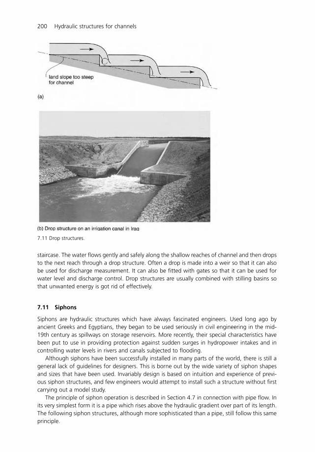
200 Hydraulic structures for channels
7.11 Drop structures.
staircase. The water flows gently and safely along the shallow reaches of channel and then dropsto the next reach through a drop structure. Often a drop is made into a weir so that it can alsobe used for discharge measurement. It can also be fitted with gates so that it can be used forwater level and discharge control. Drop structures are usually combined with stilling basins sothat unwanted energy is got rid of effectively.
7.11 Siphons
Siphons are hydraulic structures which have always fascinated engineers. Used long ago byancient Greeks and Egyptians, they began to be used seriously in civil engineering in the mid-19th century as spillways on storage reservoirs. More recently, their special characteristics havebeen put to use in providing protection against sudden surges in hydropower intakes and incontrolling water levels in rivers and canals subjected to flooding.
Although siphons have been successfully installed in many parts of the world, there is still ageneral lack of guidelines for designers. This is borne out by the wide variety of siphon shapesand sizes that have been used. Invariably design is based on intuition and experience of previ-ous siphon structures, and few engineers would attempt to install such a structure without firstcarrying out a model study.
The principle of siphon operation is described in Section 4.7 in connection with pipe flow. Inits very simplest form it is a pipe which rises above the hydraulic gradient over part of its length.The following siphon structures, although more sophisticated than a pipe, still follow this sameprinciple.
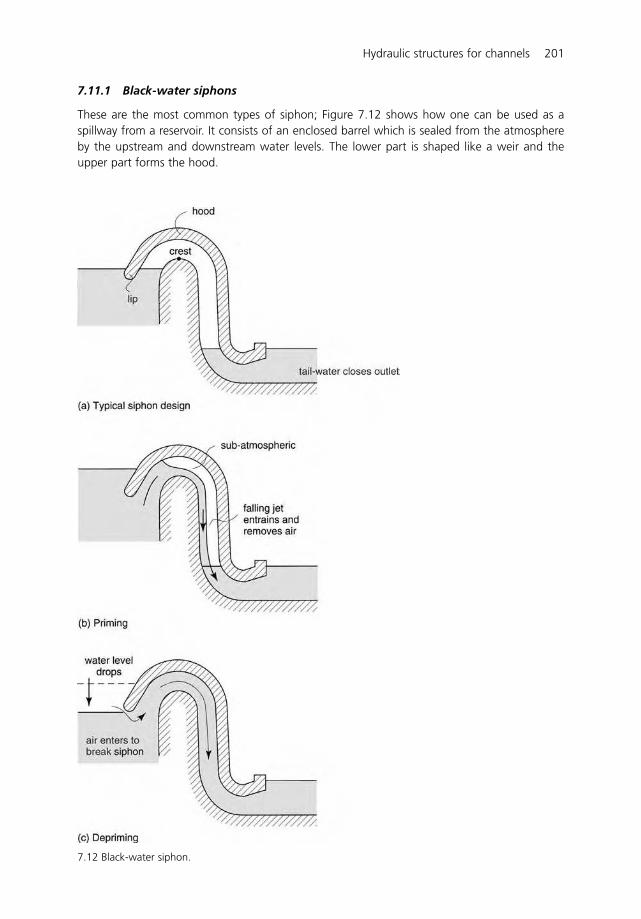
Hydraulic structures for channels 201
7.12 Black-water siphon.
7.11.1 Black-water siphons
These are the most common types of siphon; Figure 7.12 shows how one can be used as aspillway from a reservoir. It consists of an enclosed barrel which is sealed from the atmosphereby the upstream and downstream water levels. The lower part is shaped like a weir and theupper part forms the hood.
202 Hydraulic structures for channels
Water starts to flow through a siphon when the upstream water level rises above the crest. Asthe flow plunges into the downstream water it entrains and removes air from inside the barrel. Asthe barrel is sealed, air cannot enter from outside and so the pressure gradually falls and thisincreases the flow rate until the barrel is running full of water. At this stage the siphon is said to beprimed and flow is described as black-water flow. This is in contrast to the flow just before primingwhen there is a lot of air entrained and it has a white appearance. This is termed white-water flow.
Priming takes place rapidly until the discharge reaches the siphon’s full capacity. This isdetermined by the size of the barrel and the difference in energy available across the siphon.The siphon eventually starts to draw down the upstream water level and this continues evenwhen the water level falls below the crest. Only when it is drawn down to the lip on the hoodon the inlet can air enter the barrel and break the siphonic action. Flow then stops rapidly andwill only begin again when the siphon is reprimed.
Black-water siphons have several advantages over conventional spillways. There are nomoving parts such as gates and so they do not need constant attention from operators. Theyrespond automatically, and rapidly, to changes in flow and water levels and so floods whichcome unexpectedly in the night do not cause problems. Their compactness also means that theyare very useful when crest lengths for conventional weir spillways are limited. But they are notwithout problems. The abruptness of priming produces a sudden rush of water which can causeproblems downstream. They are also prone to hunting when the flow towards a siphon is lessthan the siphon capacity. They are continually priming and de-priming and this can cause surgesdownstream and vibration which is not good for the structure.
7.11.2 Air-regulated siphons
This type of siphon is a more recent development and offers many advantages over the morecommon black-water siphon. It automatically adjusts its discharge to match the approach flowand at the same time maintains a constant water level on the upstream side. This is achieved bythe siphon passing a mixture of air and water.
Air-regulated siphons are typically used for water level control in reservoirs and in rivers andcanals. They will maintain a constant water level in a channel even though the discharge ischanging. This would be an ideal structure for the wetland example discussed earlier.
Figure 7.13a shows a typical air-regulated siphon for a river. There needs to be sufficientenergy available to entrain air in the barrel and take it out to prime the siphon. This one isdesigned to operate at very low heads of 1–2 m (difference between the upstream and down-stream water levels). The siphon is shaped in many ways like a black-water siphon and relieson the barrel being enclosed and sealed by the upstream and downstream water levels. But themain difference is the inlet to the hood or upstream lip. This is set above the crest level whereasin a black-water siphon it is set below. A step is also included in the down-leg to encourageturbulence and air entrainment.
The operation of the siphon has several distinct phases (Figure 7.13 a–e):
Phase I – Free weir flow (Figure 7.13a) As the upstream water level starts to rise due toincreased flow, water flows over the crest and plunges into the downstream pool. The struc-ture behaves as a conventional free flowing weir. As the water level has not yet reached theupstream lip, air which is evacuated by the flow is immediately replaced and the pressurein the barrel remains atmospheric.Phase II – Deflected flow (Figure 7.13b and c) As the flow increases, the upstream waterlevel rises further and seals the barrel. The evacuation of air continues and a partial vac-uum is created. This raises the head of water over the crest and so increases the discharge
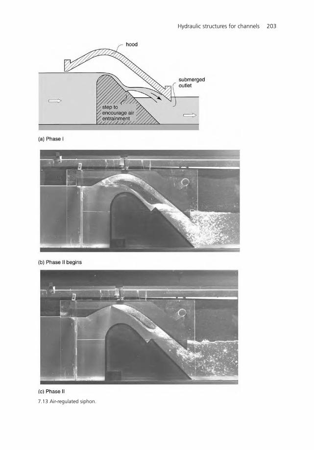
Hydraulic structures for channels 203
7.13 Air-regulated siphon.
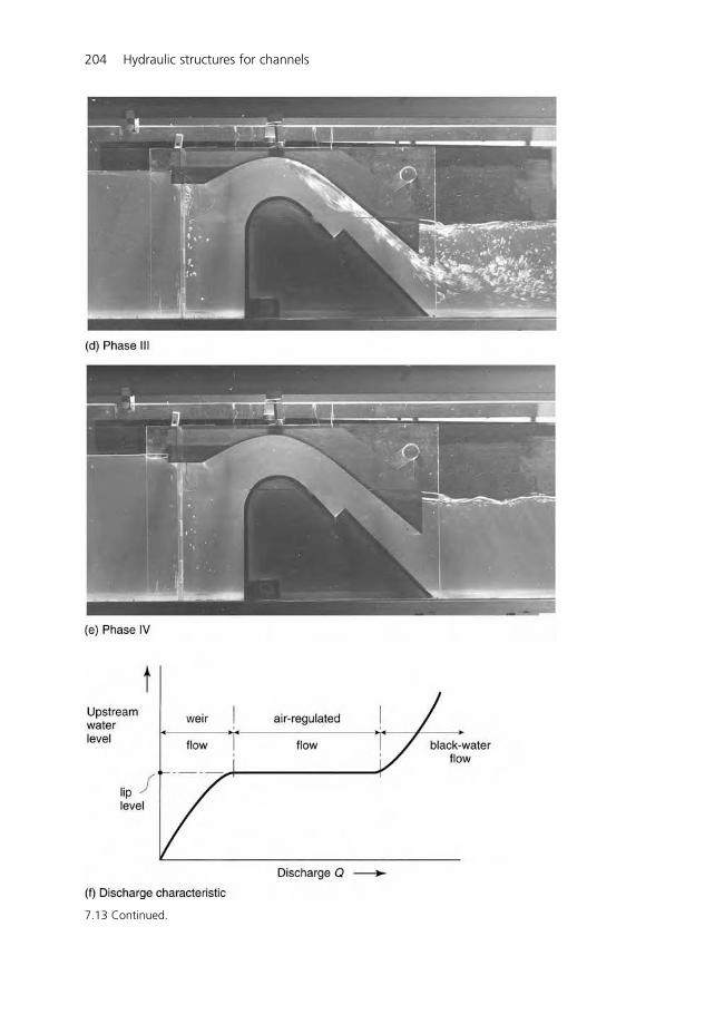
204 Hydraulic structures for channels
7.13 Continued.
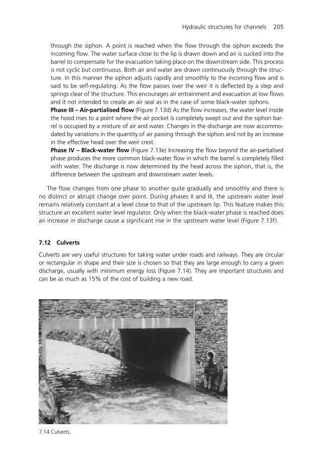
Hydraulic structures for channels 205
through the siphon. A point is reached when the flow through the siphon exceeds theincoming flow. The water surface close to the lip is drawn down and air is sucked into thebarrel to compensate for the evacuation taking place on the downstream side. This processis not cyclic but continuous. Both air and water are drawn continuously through the struc-ture. In this manner the siphon adjusts rapidly and smoothly to the incoming flow and issaid to be self-regulating. As the flow passes over the weir it is deflected by a step andsprings clear of the structure. This encourages air entrainment and evacuation at low flowsand it not intended to create an air seal as in the case of some black-water siphons.Phase III – Air-partialised flow (Figure 7.13d) As the flow increases, the water level insidethe hood rises to a point where the air pocket is completely swept out and the siphon bar-rel is occupied by a mixture of air and water. Changes in the discharge are now accommo-dated by variations in the quantity of air passing through the siphon and not by an increasein the effective head over the weir crest.Phase IV – Black-water flow (Figure 7.13e) Increasing the flow beyond the air-partialisedphase produces the more common black-water flow in which the barrel is completely filledwith water. The discharge is now determined by the head across the siphon, that is, thedifference between the upstream and downstream water levels.
The flow changes from one phase to another quite gradually and smoothly and there isno distinct or abrupt change over point. During phases II and III, the upstream water levelremains relatively constant at a level close to that of the upstream lip. This feature makes thisstructure an excellent water level regulator. Only when the black-water phase is reached doesan increase in discharge cause a significant rise in the upstream water level (Figure 7.13f).
7.12 Culverts
Culverts are very useful structures for taking water under roads and railways. They are circularor rectangular in shape and their size is chosen so that they are large enough to carry a givendischarge, usually with minimum energy loss (Figure 7.14). They are important structures andcan be as much as 15% of the cost of building a new road.
7.14 Culverts.
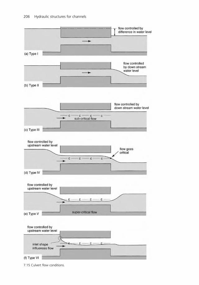
206 Hydraulic structures for channels
7.15 Culvert flow conditions.
Hydraulic structures for channels 207
Although they are very simple in appearance culverts can be quite complex hydraulicallydepending on how and where they are used. Sometimes they flow part full, like an open chan-nel and other times they can flow full, like a pipe. Six different flow conditions are recogniseddepending on the size and shape of a culvert, its length and its position in relation to theupstream and downstream water level (Figure 7.15).
The simplest condition occurs when a culvert is set well below both the upstream anddownstream water levels and it runs full of water (type I). It behaves like a pipe and the differ-ence between the water levels is the energy available which determines the discharge. This fullpipe flow can still occur even when the downstream water level falls below the culvert soffit (thisis the roof of the culvert) (type II). The culvert is now behaving like an orifice and the flow is con-trolled by the upstream water level and the size of the culvert. In both cases the discharge is con-trolled by what is happening downstream. When the water level falls the discharge increases andwhen it rises the discharge decreases. If the flow in the channel does not change then any changein the downstream water level will have a corresponding effect on the upstream water level.
The four remaining flow conditions are for open channel flow. Three occur when both theupstream and downstream water levels are below the culvert soffit (type III, IV and V). Thedifference between III and IV is the slope of the culvert. III produces sub-critical flow and sothe discharge is controlled by the downstream water level. When the downstream level risesthe discharge reduces or the upstream level rises to accommodate the same flow. In IV, theflow is still sub-critical but the downstream water level is low and so the flow goes throughthe critical depth at the outlet. This means that the flow is controlled by the upstream level.Because the flow has gone through the critical depth any changes downstream do not affectthe flow in the culvert or upstream. Condition V produces super-critical flow and so the cul-vert is again controlled by the upstream level. A rise in the downstream level will have noeffect until it starts to drown the culvert.
The final condition occurs when the upstream water level is above the soffit, the downstreamlevel is below and there is a sharp corner at the entrance causing the flow to separate ( type IV).Open channel flow occurs in the culvert and is primarily due to the shape of the entrance. Butif the entrance is rounded then this could change the flow to pipe flow. Clearly this wouldimprove its discharge capacity.
Because of their complexity, and particularly the importance of the shape of the entrance,most culvert designs are based on model tests rather than on fundamental formulae. But thisdoes not mean that every culvert must be tested in this way. There has already been extensivetesting of culverts over many years and so designers look to the standard handbooks whendeigning new culverts (see references for details).
7.13 Some examples to test your understanding
1 A broad-crested weir 3.5 m wide is to be constructed in a channel to measure a dischargeof 4.3 m3/s. When the normal depth of flow is 1.2 m, calculate the height of weir neededto measure this flow assuming that the flow must go critical on the weir crest (0.4 m).
2 A broad-crested weir is 5.0 m wide and 0.5 m high is used to measure a discharge of7.5 m3/s. Calculate the water depth upstream of the weir assuming that critical depthoccurs on the weir and there are no energy losses (1.45 m).

8 Pumps
8.1 Introduction
A few water supply systems have the benefit of a gravity supply but most require some kind ofpumping. Pumps are a means of adding energy to water. They convert fuel energy, such aspetrol or diesel, into useful water energy using combustion engines or electric motors. In thepipeline problem in Chapter 5 the energy to drive water along the pipeline to the town wasobtained from a reservoir located high above the town. The energy line drawn from the reser-voir to the town indicated the amount of energy available. Adding a pump to this systemincreases the available energy and raises the energy line so that the discharge from the reservoirto the town can be increased (Figure 8.1).
Pumps have been used for thousands of years. Early examples were largely small hand- oranimal-powered pumps for lifting small quantities of water. It was not until the advent of thesteam engine, only two centuries ago, that the larger rotating pumps were developed andbecame an important part of the study of hydraulics. Consequently there are two main types ofpump:
� Positive displacement pumps – these are mainly small hand- and animal-powered pumpsmany of which are still used today;
� Roto-dynamic pumps – these are mainly the modern pumps driven by diesel or electricmotors that are now in common use throughout the world.
8.1 Pumps add energy to pipe systems
Because of the similarities between pumps and turbines (used to generate energy) a smallsection is devoted to them at the end of this chapter.
8.2 Positive displacement pumps
Positive displacement pumps usually deliver small discharges over a wide range of pumpingheads. Typical examples are hand-piston pumps, rotary pumps, air-lift pumps and Archimedeanscrews (Figure 8.2).
Hand-piston pumps are used extensively in developing countries for lifting groundwater fordomestic water supplies. A pipe connects the pump to the water source – usually a well. At theend of this pipe is a non-return valve that only allows water to enter the pump and stops itfrom flowing back into the source. The pump itself comprises a piston and cylinder. Thesemust have a very close fit so that when the piston is raised, it creates a vacuum in the cylinderand water is drawn up into the pump. When the piston is pushed down the water is pushedthrough a small valve in the piston to fill up the space above it. As the piston is raised again, itlifts the water above it so it pores out through the spout of the pump and into a tank or otherwater collecting device. The procedure is then repeated. The discharge from the pumpdepends on the energy available from those working the pump handle. You basically get outwhat you put in. The height to which water can be pumped in this way is fixed only by thestrength of those pumping and the pump seals, which will start to leak when the pressure getstoo high.
The rotary pump contains two gears that mesh together as they rotate in opposite directions.The liquid becomes trapped between the gears and is forced into the delivery pipe.
The air-lift pump uses an air compressor to force air down a pipe into the inlet of the waterpipe. The mixture of air and water, which is less dense than the surrounding water in the well,then rises up above ground level. This pump is not very efficient but it will pump water that hassand and grit in it which would normally damage other pumps.
The Archimedean screw pump has been used for thousands of years and is still used todayfor pumping irrigation water in Egypt. It comprises a helical screw inside a casing. Water is liftedby turning the screw by hand. Some modern pumping stations also use this idea but the screwsare much larger and are driven by a diesel or electric power unit.
The treadle pump is another example of positive displacement pump (Figure 8.3). It isgrowing in popularity in many developing countries because it enables poor farmers, whocannot afford a motor-driven pump, to use their human power to pump the large volumesof water needed for irrigating crops. It was first developed in Bangladesh in the early 1980sfor irrigating flooded rice and it is now estimated that some two million pumps are in usethroughout Asia. Their popularity has spread in recent years to sub-Saharan Africa. Thedesigners of the treadle pump have skilfully adapted the principle of the hand-piston pumpso that greater volumes of water can be lifted. Two pistons and cylinders are used to raisewater instead of one. But the most important innovation was the change in driving powerfrom arms and hands to legs and feet. Leg muscles are much more powerful than armmuscles and so they are capable of lifting much more water. The two cylinders 0.75 to110 mm in diameter, are located side-by-side and a chain or rope, which passes over a pulley,connects the two pistons together so that when one piston is being pushed down, the otherone is being raised. Each piston is connected to a treadle on which the operator stands andpushes them up and down in a rhythmic motion – like pushing peddles on a bicycle. Thisrhythmic method of driving the pump seems to have gained wide acceptance among farmersin the developing world.
Although the pump is popular in several developing countries some exaggerated claims areoften made about its physical performance, usually by those who have little knowledge of how
Pumps 209
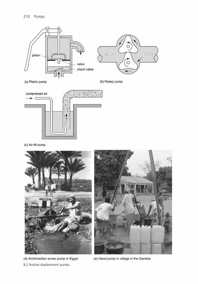
210 Pumps
(d) Archimedian screw pump in Egypt (e) Hand pump in village in the Gambia
8.2 Positive displacement pumps.
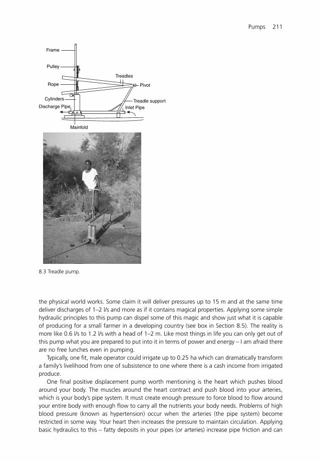
the physical world works. Some claim it will deliver pressures up to 15 m and at the same timedeliver discharges of 1–2 l/s and more as if it contains magical properties. Applying some simplehydraulic principles to this pump can dispel some of this magic and show just what it is capableof producing for a small farmer in a developing country (see box in Section 8.5). The reality ismore like 0.6 l/s to 1.2 l/s with a head of 1–2 m. Like most things in life you can only get out ofthis pump what you are prepared to put into it in terms of power and energy – I am afraid thereare no free lunches even in pumping.
Typically, one fit, male operator could irrigate up to 0.25 ha which can dramatically transforma family’s livelihood from one of subsistence to one where there is a cash income from irrigatedproduce.
One final positive displacement pump worth mentioning is the heart which pushes bloodaround your body. The muscles around the heart contract and push blood into your arteries,which is your body’s pipe system. It must create enough pressure to force blood to flow aroundyour entire body with enough flow to carry all the nutrients your body needs. Problems of highblood pressure (known as hypertension) occur when the arteries (the pipe system) becomerestricted in some way. Your heart then increases the pressure to maintain circulation. Applyingbasic hydraulics to this – fatty deposits in your pipes (or arteries) increase pipe friction and can
Pumps 211
Frame
Pulley
Treadles
Pivot
Treadle supportInlet PipeDischarge Pipe
Mainfold
Rope
Cylinders
8.3 Treadle pump.
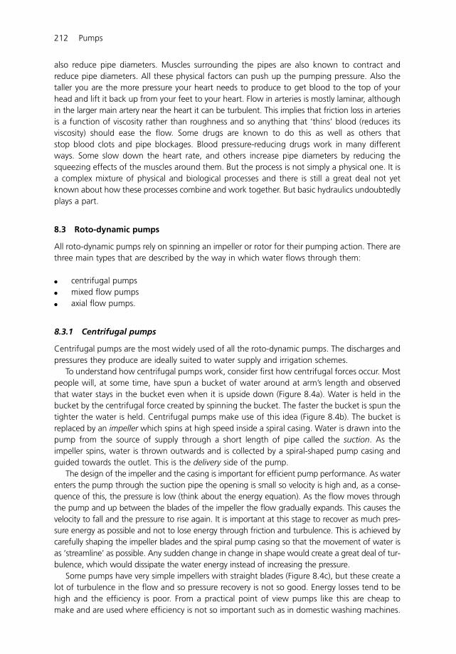
also reduce pipe diameters. Muscles surrounding the pipes are also known to contract andreduce pipe diameters. All these physical factors can push up the pumping pressure. Also thetaller you are the more pressure your heart needs to produce to get blood to the top of yourhead and lift it back up from your feet to your heart. Flow in arteries is mostly laminar, althoughin the larger main artery near the heart it can be turbulent. This implies that friction loss in arteriesis a function of viscosity rather than roughness and so anything that ‘thins’ blood (reduces itsviscosity) should ease the flow. Some drugs are known to do this as well as others thatstop blood clots and pipe blockages. Blood pressure-reducing drugs work in many differentways. Some slow down the heart rate, and others increase pipe diameters by reducing thesqueezing effects of the muscles around them. But the process is not simply a physical one. It isa complex mixture of physical and biological processes and there is still a great deal not yetknown about how these processes combine and work together. But basic hydraulics undoubtedlyplays a part.
8.3 Roto-dynamic pumps
All roto-dynamic pumps rely on spinning an impeller or rotor for their pumping action. There arethree main types that are described by the way in which water flows through them:
� centrifugal pumps� mixed flow pumps� axial flow pumps.
8.3.1 Centrifugal pumps
Centrifugal pumps are the most widely used of all the roto-dynamic pumps. The discharges andpressures they produce are ideally suited to water supply and irrigation schemes.
To understand how centrifugal pumps work, consider first how centrifugal forces occur. Mostpeople will, at some time, have spun a bucket of water around at arm’s length and observedthat water stays in the bucket even when it is upside down (Figure 8.4a). Water is held in thebucket by the centrifugal force created by spinning the bucket. The faster the bucket is spun thetighter the water is held. Centrifugal pumps make use of this idea (Figure 8.4b). The bucket isreplaced by an impeller which spins at high speed inside a spiral casing. Water is drawn into thepump from the source of supply through a short length of pipe called the suction. As theimpeller spins, water is thrown outwards and is collected by a spiral-shaped pump casing andguided towards the outlet. This is the delivery side of the pump.
The design of the impeller and the casing is important for efficient pump performance. As waterenters the pump through the suction pipe the opening is small so velocity is high and, as a conse-quence of this, the pressure is low (think about the energy equation). As the flow moves throughthe pump and up between the blades of the impeller the flow gradually expands. This causes thevelocity to fall and the pressure to rise again. It is important at this stage to recover as much pres-sure energy as possible and not to lose energy through friction and turbulence. This is achieved bycarefully shaping the impeller blades and the spiral pump casing so that the movement of water isas ‘streamline’ as possible. Any sudden change in change in shape would create a great deal of tur-bulence, which would dissipate the water energy instead of increasing the pressure.
Some pumps have very simple impellers with straight blades (Figure 8.4c), but these create alot of turbulence in the flow and so pressure recovery is not so good. Energy losses tend to behigh and the efficiency is poor. From a practical point of view pumps like this are cheap tomake and are used where efficiency is not so important such as in domestic washing machines.
212 Pumps
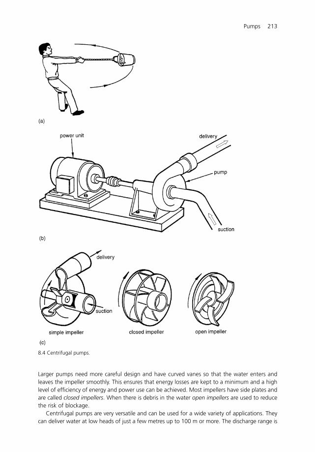
Larger pumps need more careful design and have curved vanes so that the water enters andleaves the impeller smoothly. This ensures that energy losses are kept to a minimum and a highlevel of efficiency of energy and power use can be achieved. Most impellers have side plates andare called closed impellers. When there is debris in the water open impellers are used to reducethe risk of blockage.
Centrifugal pumps are very versatile and can be used for a wide variety of applications. Theycan deliver water at low heads of just a few metres up to 100 m or more. The discharge range is
Pumps 213
8.4 Centrifugal pumps.
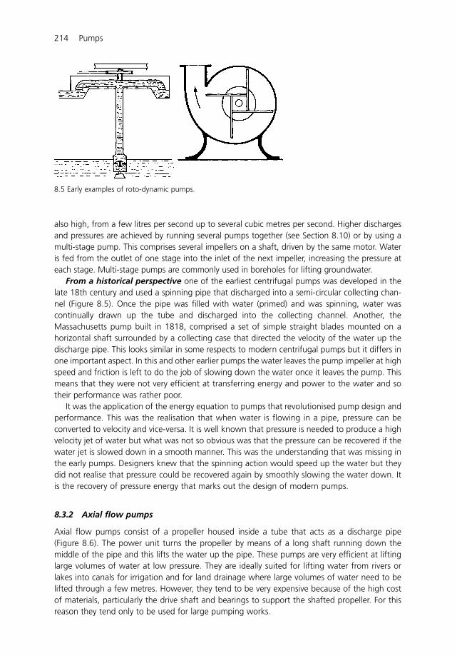
also high, from a few litres per second up to several cubic metres per second. Higher dischargesand pressures are achieved by running several pumps together (see Section 8.10) or by using amulti-stage pump. This comprises several impellers on a shaft, driven by the same motor. Wateris fed from the outlet of one stage into the inlet of the next impeller, increasing the pressure ateach stage. Multi-stage pumps are commonly used in boreholes for lifting groundwater.
From a historical perspective one of the earliest centrifugal pumps was developed in thelate 18th century and used a spinning pipe that discharged into a semi-circular collecting chan-nel (Figure 8.5). Once the pipe was filled with water (primed) and was spinning, water wascontinually drawn up the tube and discharged into the collecting channel. Another, theMassachusetts pump built in 1818, comprised a set of simple straight blades mounted on ahorizontal shaft surrounded by a collecting case that directed the velocity of the water up thedischarge pipe. This looks similar in some respects to modern centrifugal pumps but it differs inone important aspect. In this and other earlier pumps the water leaves the pump impeller at highspeed and friction is left to do the job of slowing down the water once it leaves the pump. Thismeans that they were not very efficient at transferring energy and power to the water and sotheir performance was rather poor.
It was the application of the energy equation to pumps that revolutionised pump design andperformance. This was the realisation that when water is flowing in a pipe, pressure can beconverted to velocity and vice-versa. It is well known that pressure is needed to produce a highvelocity jet of water but what was not so obvious was that the pressure can be recovered if thewater jet is slowed down in a smooth manner. This was the understanding that was missing inthe early pumps. Designers knew that the spinning action would speed up the water but theydid not realise that pressure could be recovered again by smoothly slowing the water down. Itis the recovery of pressure energy that marks out the design of modern pumps.
8.3.2 Axial flow pumps
Axial flow pumps consist of a propeller housed inside a tube that acts as a discharge pipe(Figure 8.6). The power unit turns the propeller by means of a long shaft running down themiddle of the pipe and this lifts the water up the pipe. These pumps are very efficient at liftinglarge volumes of water at low pressure. They are ideally suited for lifting water from rivers orlakes into canals for irrigation and for land drainage where large volumes of water need to belifted through a few metres. However, they tend to be very expensive because of the high costof materials, particularly the drive shaft and bearings to support the shafted propeller. For thisreason they tend only to be used for large pumping works.
214 Pumps
8.5 Early examples of roto-dynamic pumps.
8.3.3 Mixed flow pumps
These pumps are a mixture of axial flow and centrifugal pumps and so combine the best features ofboth pump types. Mixed flow pumps are more efficient at pumping larger quantities of water thancentrifugal pumps and are more efficient at pumping to higher pressures than axial flow pumps.
8.4 Pumping pressure
8.4.1 Suction lift
Pumps are usually located above the water source for the convenience of the users and thisleads to the idea that pumps must ‘suck’ up water from the source before lifting it to somehigher level. But this idea and the word ‘sucking’ can lead to misunderstandings about howpumps work (Figure 8.7).
‘Sucking’ water up a drinking straw is very similar to the way a pump draws water from asource. However, you do not actually suck up the water, you suck out the air from the straw andcreate a vacuum. Atmospheric pressure does the rest. It pushes down on the water surface inthe glass and forces water up the straw to fill the vacuum. So atmospheric pressure provides thedriving force but it also puts a limit on how high water can be lifted in this way. It does notdepend on the ability of the sucker. At sea level, atmospheric pressure is approximately 10 m
Pumps 215
8.6 Axial flow pump.
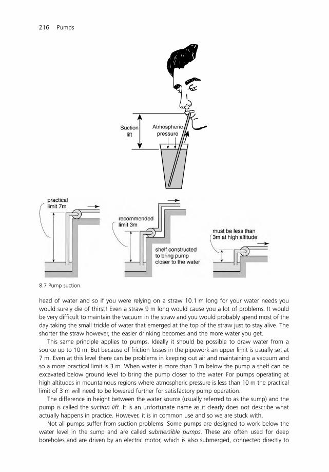
head of water and so if you were relying on a straw 10.1 m long for your water needs youwould surely die of thirst! Even a straw 9 m long would cause you a lot of problems. It wouldbe very difficult to maintain the vacuum in the straw and you would probably spend most of theday taking the small trickle of water that emerged at the top of the straw just to stay alive. Theshorter the straw however, the easier drinking becomes and the more water you get.
This same principle applies to pumps. Ideally it should be possible to draw water from asource up to 10 m. But because of friction losses in the pipework an upper limit is usually set at7 m. Even at this level there can be problems in keeping out air and maintaining a vacuum andso a more practical limit is 3 m. When water is more than 3 m below the pump a shelf can beexcavated below ground level to bring the pump closer to the water. For pumps operating athigh altitudes in mountainous regions where atmospheric pressure is less than 10 m the practicallimit of 3 m will need to be lowered further for satisfactory pump operation.
The difference in height between the water source (usually referred to as the sump) and thepump is called the suction lift. It is an unfortunate name as it clearly does not describe whatactually happens in practice. However, it is in common use and so we are stuck with.
Not all pumps suffer from suction problems. Some pumps are designed to work below thewater level in the sump and are called submersible pumps. These are often used for deepboreholes and are driven by an electric motor, which is also submerged, connected directly to
216 Pumps
Suctionlift
Atmosphericpressure
8.7 Pump suction.
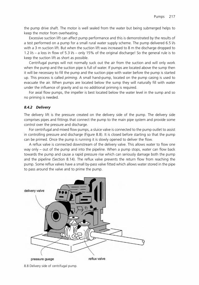
the pump drive shaft. The motor is well sealed from the water but being submerged helps tokeep the motor from overheating.
Excessive suction lift can affect pump performance and this is demonstrated by the results ofa test performed on a pump for a small rural water supply scheme. The pump delivered 6.5 l/swith a 3 m suction lift. But when the suction lift was increased to 8 m the discharge dropped to1.2 l/s – a loss in flow of 5.3 l/s – only 15% of the original discharge! So the general rule is tokeep the suction lift as short as possible.
Centrifugal pumps will not normally suck out the air from the suction and will only workwhen the pump and the suction pipe is full of water. If pumps are located above the sump thenit will be necessary to fill the pump and the suction pipe with water before the pump is startedup. This process is called priming. A small hand-pump, located on the pump casing is used toevacuate the air. When pumps are located below the sump they will naturally fill with waterunder the influence of gravity and so no additional priming is required.
For axial flow pumps, the impeller is best located below the water level in the sump and sono priming is needed.
8.4.2 Delivery
The delivery lift is the pressure created on the delivery side of the pump. The delivery sidecomprises pipes and fittings that connect the pump to the main pipe system and provide somecontrol over the pressure and discharge.
For centrifugal and mixed flow pumps, a sluice valve is connected to the pump outlet to assistin controlling pressure and discharge (Figure 8.8). It is closed before starting so that the pumpcan be primed. Once the pump is running it is slowly opened to deliver the flow.
A reflux valve is connected downstream of the delivery valve. This allows water to flow oneway only – out of the pump and into the pipeline. When a pump stops, water can flow backtowards the pump and cause a rapid pressure rise which can seriously damage both the pumpand the pipeline (Section 8.14). The reflux valve prevents the return flow from reaching thepump. Some reflux valves have a small by-pass valve fitted which allows water stored in the pipeto pass around the valve and to prime the pump.
Pumps 217
8.8 Delivery side of centrifugal pump.
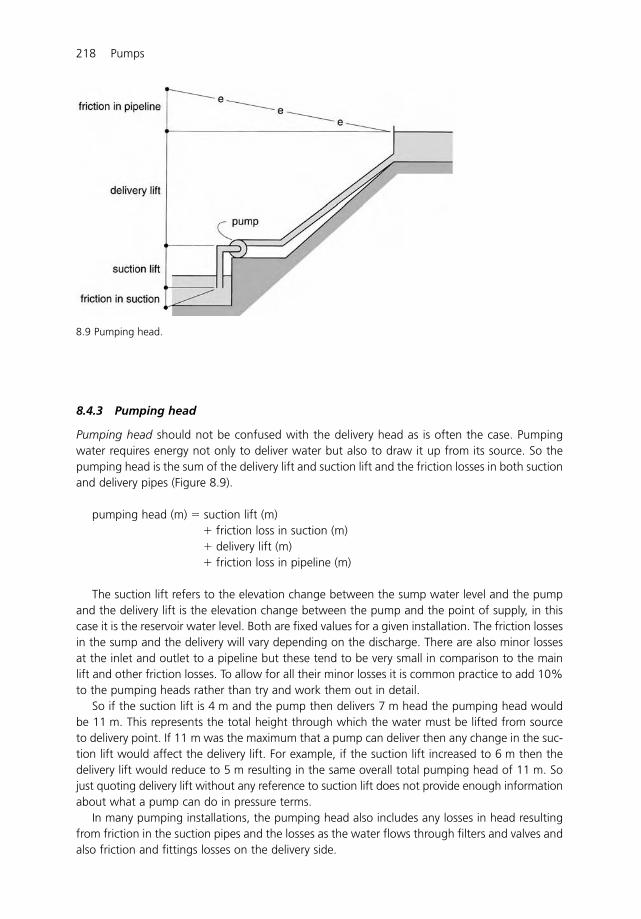
8.4.3 Pumping head
Pumping head should not be confused with the delivery head as is often the case. Pumpingwater requires energy not only to deliver water but also to draw it up from its source. So thepumping head is the sum of the delivery lift and suction lift and the friction losses in both suctionand delivery pipes (Figure 8.9).
pumping head (m) � suction lift (m)� friction loss in suction (m)� delivery lift (m)� friction loss in pipeline (m)
The suction lift refers to the elevation change between the sump water level and the pumpand the delivery lift is the elevation change between the pump and the point of supply, in thiscase it is the reservoir water level. Both are fixed values for a given installation. The friction lossesin the sump and the delivery will vary depending on the discharge. There are also minor lossesat the inlet and outlet to a pipeline but these tend to be very small in comparison to the mainlift and other friction losses. To allow for all their minor losses it is common practice to add 10%to the pumping heads rather than try and work them out in detail.
So if the suction lift is 4 m and the pump then delivers 7 m head the pumping head wouldbe 11 m. This represents the total height through which the water must be lifted from sourceto delivery point. If 11 m was the maximum that a pump can deliver then any change in the suc-tion lift would affect the delivery lift. For example, if the suction lift increased to 6 m then thedelivery lift would reduce to 5 m resulting in the same overall total pumping head of 11 m. Sojust quoting delivery lift without any reference to suction lift does not provide enough informationabout what a pump can do in pressure terms.
In many pumping installations, the pumping head also includes any losses in head resultingfrom friction in the suction pipes and the losses as the water flows through filters and valves andalso friction and fittings losses on the delivery side.
218 Pumps
8.9 Pumping head.
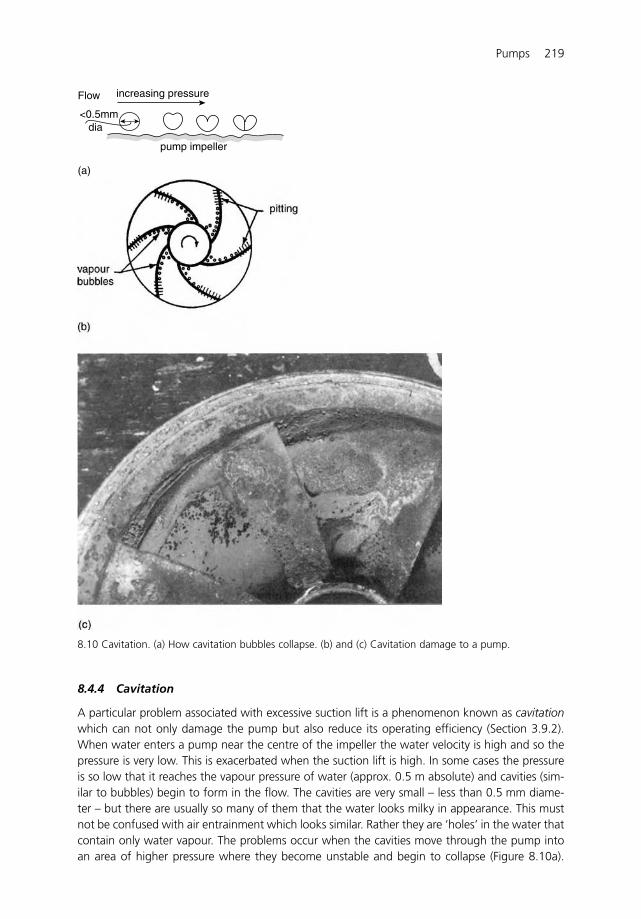
8.4.4 Cavitation
A particular problem associated with excessive suction lift is a phenomenon known as cavitationwhich can not only damage the pump but also reduce its operating efficiency (Section 3.9.2).When water enters a pump near the centre of the impeller the water velocity is high and so thepressure is very low. This is exacerbated when the suction lift is high. In some cases the pressureis so low that it reaches the vapour pressure of water (approx. 0.5 m absolute) and cavities (sim-ilar to bubbles) begin to form in the flow. The cavities are very small – less than 0.5 mm diame-ter – but there are usually so many of them that the water looks milky in appearance. This mustnot be confused with air entrainment which looks similar. Rather they are ‘holes’ in the water thatcontain only water vapour. The problems occur when the cavities move through the pump intoan area of higher pressure where they become unstable and begin to collapse (Figure 8.10a).
Pumps 219
increasing pressure
pump impeller
(a)
Flow
<0.5mmdia
8.10 Cavitation. (a) How cavitation bubbles collapse. (b) and (c) Cavitation damage to a pump.
A small needle jet of water rushes across the cavity with such force that if the cavity is close tothe pump impeller or casing then it can start to damage them. Each cavity collapse is notsignificant on its own but when many thousands of them continually collapse close to the metalsurfaces then damage begins to grow. In some cases it has been known to completely wear awaythe impeller blades (Figure 8.10b).
Most pumps in fact cavitate but not all cavitation causes damage. Pump designers go togreat lengths to ensure that the cavities collapse in the main flow, well away from the impellerblades. If this is not possible then stainless steel impellers are used as this is one of the few mate-rials which can resist cavitation damage. But this is a very expensive option and not one to takeup lightly.
Cavitation not only erodes the surfaces in contact with water but it can also be very noisy.It also causes vibration and can reduce pumping efficiency. If you have an opportunity tovisit a water pumping station then place your ear against the pump casing and you will hearthe cavitation. Above all the noise of the pump engines it should be possible to hear a sharpcrackling sound. This is the sound of the cavities collapsing as the pressure rises in the pump.The level of the noise produced by the cavitation is a measure of how badly the pump iscavitating.
Cavitation also occurs in turbine runners which are discussed briefly later in this chapter. Highvelocities at the turbine inlet produce cavities which then collapse close to the runner bladesnear the exit.
A concept sometimes used for limiting suction lift and so avoiding cavitation is the NetPositive Suction Head (NPSH). Manufacturers normally specify a value of NPSH for each dischargeto ensure a pump operates satisfactorily.
The NPSH for an installation can be calculated as follows:
NPSH � Pa – Hs – Vp – hf
where Pa is atmospheric pressure (m); Hs is suction head (m); Vp is the vapour pressure of water(approx. 0.5 m absolute); hf is the head loss in the suction pipe (approx. 0.75 m).
The value of NPSH calculated using this formula must be greater than that quoted by thepump manufacturer for the pump to operate satisfactorily.
8.5 Energy for pumping
Energy is needed to pump water. The amount required depends on both the volume ofwater pumped and the height to which it is lifted. It can be calculated using the followingformula:
water energy (kWh) �
A derivation of this formula is shown in the box for the more inquisitive reader.
volume (m3) � head (m)367
220 Pumps
DERIVATION: A FORMULA TO CALCULATE ENERGY FOR PUMPING
Derive a formula to calculate the amount of energy needed to lift a volume of water V m3
to a height of H m.
Start with the basic equation for calculating energy from Section 1.10:
water energy � work done
So:
water energy (Nm) � force (N) � distance (m)
We now need to establish what the values of force and distance mean in terms ofpumping water. Look first at force. This is the total weight of water to be lifted.Usually the volume is known and so we use Newton’s second law to determine theweight:
force � mass (kg) � acceleration (m/s2)
In this case acceleration is due to gravity and so:
mass of water � volume (m3) � density (kg/m3)
So:
force � volume (m3) � density (kg/m3) � gravity constant (m/s2)
Now density � � 1000 kg/m3 and the gravity constant g � 9.81 m/s2 so:
force � volume (m3) � 1000 � 9.81� volume (m3) � 9810
The ‘distance’ part of the energy equation is the pumping head and so:
distance � pumping head (m)
Putting the values for force and distance in the energy equation:
water energy (Nm) � volume (m3) � 9810 � head (m)
But this is in Nm. We need to convert this to more useful and practical units of energy likekWh so:
1 kWh � 3 600 000 Nm (Section 1.10.2)
So:
water energy (kWh)
This simplifies to the formula which is most often used:
water energy (kWh) �volume (m3) � head (m)
367
� volume (m3) � 9810 � head (m)
3 600 000
Pumps 221
An example of how to use this formula for calculating energy for pumping is shown in the nextbox.
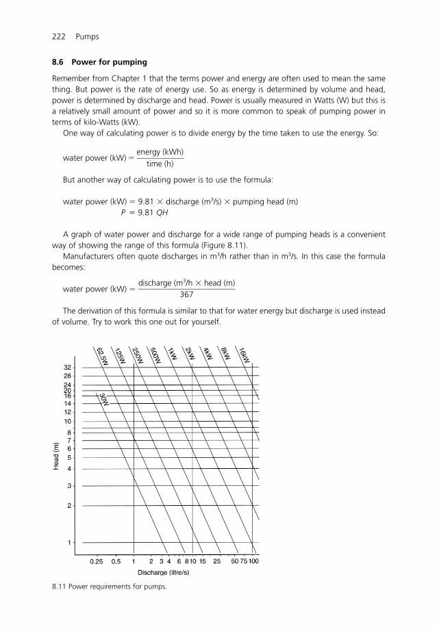
222 Pumps
8.11 Power requirements for pumps.
8.6 Power for pumping
Remember from Chapter 1 that the terms power and energy are often used to mean the samething. But power is the rate of energy use. So as energy is determined by volume and head,power is determined by discharge and head. Power is usually measured in Watts (W) but this isa relatively small amount of power and so it is more common to speak of pumping power interms of kilo-Watts (kW).
One way of calculating power is to divide energy by the time taken to use the energy. So:
But another way of calculating power is to use the formula:
water power (kW) � 9.81 � discharge (m3/s) � pumping head (m)P � 9.81 QH
A graph of water power and discharge for a wide range of pumping heads is a convenientway of showing the range of this formula (Figure 8.11).
Manufacturers often quote discharges in m3/h rather than in m3/s. In this case the formulabecomes:
water power (kW)
The derivation of this formula is similar to that for water energy but discharge is used insteadof volume. Try to work this one out for yourself.
� discharge (m3/h � head (m)
367
water power (kW) �energy (kWh)
time (h)
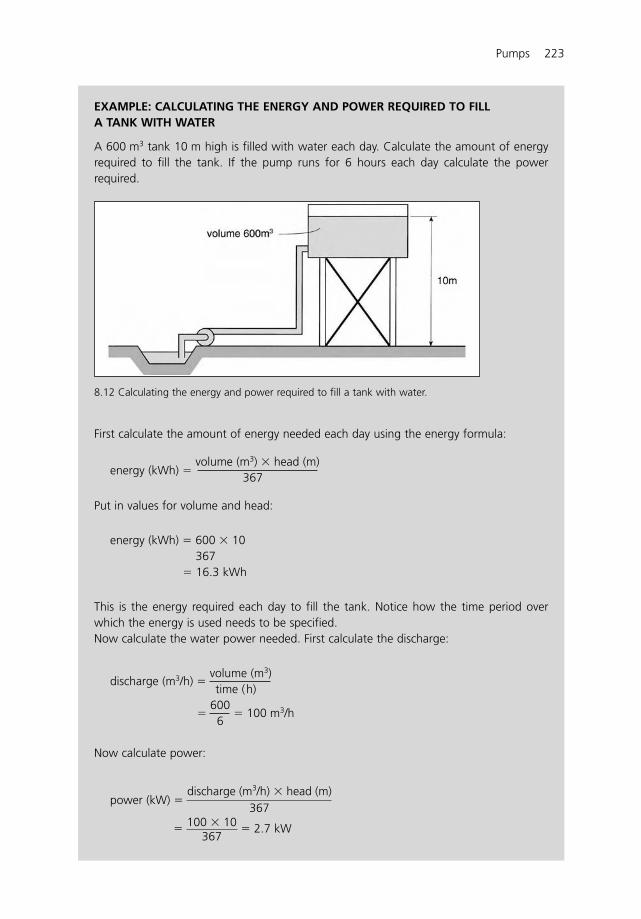
Pumps 223
EXAMPLE: CALCULATING THE ENERGY AND POWER REQUIRED TO FILL A TANK WITH WATER
A 600 m3 tank 10 m high is filled with water each day. Calculate the amount of energyrequired to fill the tank. If the pump runs for 6 hours each day calculate the powerrequired.
First calculate the amount of energy needed each day using the energy formula:
energy (kWh) �volume (m3) � head (m)
367
Put in values for volume and head:
energy (kWh) � 600 � 10367
� 16.3 kWh
This is the energy required each day to fill the tank. Notice how the time period overwhich the energy is used needs to be specified.Now calculate the water power needed. First calculate the discharge:
discharge (m3/h) �volume (m3)time (h)
�600
� 100 m3/h6
Now calculate power:
power (kW)
� 2.7 kW� 100 � 10367
� discharge (m3/h) � head (m)
367
8.12 Calculating the energy and power required to fill a tank with water.
8.6.1 Efficiency
In the example in the box the ‘water energy’ and ‘water power’ are only part of what is neededto actually fill the water tank. Losses occur in the power unit that drives the pump and in thepump itself and these need to be taken into account when the total power needed for pump-ing is determined. Energy and power losses occur when fuel energy is converted into usefulwater energy and through turbulence and friction in the pump and fittings. Much of this is dis-sipated as heat energy. The losses that occur are expressed as an efficiency, which can be lookedat from both a power and an energy point of view.
Energy and power efficiencies are often assumed to be the same. In practice this may not bethe case. A seasonal assessment of energy use efficiency may not always give the same value aspower use efficiency measured only one or two times during a lengthy period of operation.
Power efficiency is a measure of how well the power from the power unit is converted intouseful water power in the pump and is calculated as follows:
Energy use efficiency is used to judge how well a pump is performing over a longer periodof time.
To calculate energy efficiency, the time over which the energy is used must be known, forexample, a day, month or a season.
A system with no energy losses would have an efficiency of 100%, so all the power orenergy input would be transferred to the water. But this does not happen in practice. Thereare always losses in the various components of the power unit and pump, as well as in thepipe system. The actual efficiency will be the product of the efficiency of each component.For example, a centrifugal pump with an efficiency of 80% being driven by an electric motorwith an efficiency of 80% would have an overall efficiency of 64% (0.8 � 0.8 � 0.64). Theefficiency of the pipe system can be incorporated in a similar way. So it is not just the effi-ciency of the pump that matters – all the components of the system must be well matchedto produce a high overall efficiency. Just to complicate matters, the efficiency of each com-ponent is not fixed – the values vary depending on the discharge and pressure in the system.The designer’s objective is to match the various components so that together they produce
energy efficiency (%) � water energy outputactual energy input
� 100
power efficiency (%) � water power outputactual power input
� 100
224 Pumps
The energy can also be calculated from power by multiplying power by the time overwhich the power is used. In this case the time is 6 hours.
energy (kWh) � water power (kW) x operating time (h)� 2.7 � 6� 16.3 kWh
Note the two approaches produce the same answer.
Pumps 225
EXAMPLE: ESTIMATING THE DISCHARGE AND PRESSURE THAT CAN BEACHIEVED WITH A TREADLE PUMP
Estimate the discharge and pressures that can be expected from a treadle pump operatedby a farmer in a developing country (Section 8.2). Make reasonable assumptions tocomplete the calculations.
The first step is to determine the power available for pumping. Once this is establishedit is possible to determine the pressure and discharge that could be expected from thepump.
A reasonably fit, well-fed male between 20 and 40 could produce a steady poweroutput of 75 Watts for long periods. To give you some idea of what this means, it is likewalking up and down a flight of stairs in about 20 s. Not so bad for the first few times butthink about sustaining this over several hours. In a developing country where operators maynot be so well fed, or operators are women and children, a more reasonable power valuemight be 30 Watts.
The pump unit is also not very efficient at converting human power into water powerso we need to allow for an efficiency of say 40%.
So taking these figures into account assume the power input is 30 Watts (0.03 kW)and the pump efficiency is 40%:
water power (kW)
0.03 � 0.4
Power is directly related to both discharge and head so at the same power input level, ifhead increases then discharge will decrease and vice-versa.
So assume the suction lift is 2 m which is typical for many treadle pump applications.Now calculate the discharge using the above power formula:
� 0.6 l/s
If the water lift is reduced to 1 m the discharge increases:
discharge � 1.2 l/s
So when the pumping head is low the discharge ranges from 0. 6 to 1.2 l/s.
discharge � 0.03 � 0.4 � 3672
� 2.20 m3/h
� discharge (m3/h) � head (m)
367
� discharge (m3/h) � head (m)
367
the highest level of overall efficiency at the desired pressure and discharge. Usually this is notone fixed point but a range of pressures and discharges in which it is judged that the systemis performing optimally with minimal energy losses.
This is true for all lifting devices and not just centrifugal pumps. Treadle pumps, for example,have an optimum treadling speed that minimises losses and power inputs from an operator andmaximises pump output in terms of pressure and discharge.
226 Pumps
In some countries treadle pumps are used to pump water to much higher heads than this,but there is a limit to this which depends on the operator. The maximum pressure is deter-mined by the weight of the operator who stands on the treadle and applies a downwardforce on the pistons.
So assume a typical 65 kg operator standing on a treadle immediately above a typical100 mm diameter piston. Now calculate the pressure using:
Calculate the force and the area:
max. force from operator (N) � mass of operator (kg) � gravity constant (m/s2)� 65 � 9.81� 637 N
Put values for force and area into the formula to calculate pressure:
Calculate this in terms of head (m) using the pressure-head equation:
P � �gh
So the maximum head this operator can achieve pressing his full weight onto each pistonis 9 m. In practice not all operators put their full weight on the treadles and so the actualpressure may be much lower than this, say 5 m. The pressure can be increased by reduc-ing the diameter of the pistons but this will also reduce the volume of water lifted eachpump stoke. Another way of course, would be to get a heavier operator or perhaps usetwo operators at the same time, which is often done when children are using it.
If the maximum pressure that can realistically be achieved on this pump is 5 m then insuch circumstances, the water power formula shows that the discharge would be reducedto 0. 24 l/s.
Three important points to note:First, the pumping head is the sum of the suction lift and the delivery lift and so it is the
pumping head that is 5 m. Treadle pump suppliers are notorious for quoting delivery andsuction lifts separately and this can confuse the buyer who is trying to compare pump per-formance.
Second, it is clear that you cannot have both high pressure and a large discharge. Youcan have one or the other and the combination depends on the power available from
� 91 0001000 � 9.81
� 9.27 m
head (m) � P�g
pressure � 6370.007
� 91 000 N/m2
area of piston � ��d2
4 �
��0.12
4 � 0.007 m2
pressure (N/m2) � force (N/m2)
area (m2)
Pumps 227
8.7 Roto-dynamic pump performance
Small centrifugal pumps are sometimes characterised by the power of their drive motors, forexample, 3 HP pump or a 5 kW pump; or by their delivery diameter, for example, 50 mm pump(Table 8.1). This provides some guidance for selection but the full performance characteristicsshould be used for larger pumps.
All roto-dynamic pumps are factory tested and data are published by the manufacturers onthe following characteristics:
� discharge and head� discharge and power� discharge and efficiency.
These data are usually presented graphically; typical characteristics for all three pump types areshown in Figure 8.13. The curves shown are only for one operating speed. But as pumpscan run at many different speeds, several graphs are needed to show their full performancepossibilities.
8.7.1 Discharge and head
The relationship between discharge and head is usually of most immediate concern to the user.Will the pump deliver the discharge at the required pressure? A pump can, in fact, deliver a widerange of discharges but there will be changes in pressure as the discharge changes. Pump speedcan also be varied and this changes both head and discharge. The faster the speed the greaterwill be the head and discharge.
Figure 8.13a shows typical discharge – head curves for centrifugal, mixed flow and axialflow pumps for a given pump speed. The axes of the graph would normally show discharge(in m3/s) and head (in m). But in order to show typical changes in performance the curves havebeen drawn to show the percentage changes when either the discharge or the head ischanged from the normal operating condition represented by the 100% point. So for the cen-trifugal pump, when the discharge is reduced to 80% of its design flow the head increases to
Table 8.1 Typical discharges from smallcentrifugal pumps.
Pump size (mm) Discharge (litre/s)
25 0–550 5–1575 15–25100 25–35125 35–50
operator. Basically there is no ‘free lunch’ – you get out of the pump what you areprepared to put into it.
Finally, this is not rocket science. But it does demonstrate how basic hydraulics can beapplied usefully to design what is a simple but very effective water lifting device – somethingthat is not always done in practice.
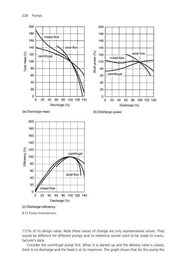
228 Pumps
8.13 Pump characteristics.
112% of its design value. Note these values of change are only representative values. Theywould be different for different pumps and so reference would need to be made to manu-facturer’s data.
Consider the centrifugal pump first. When it is started up and the delivery valve is closed,there is no discharge and the head is at its maximum. The graph shows that for this pump the
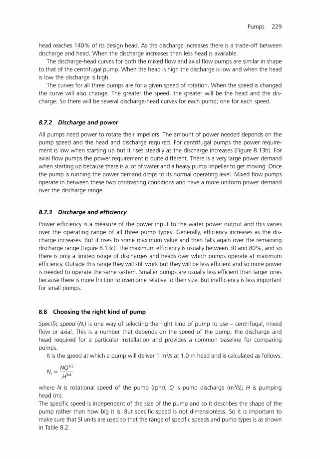
Pumps 229
head reaches 140% of its design head. As the discharge increases there is a trade-off betweendischarge and head. When the discharge increases then less head is available.
The discharge-head curves for both the mixed flow and axial flow pumps are similar in shapeto that of the centrifugal pump. When the head is high the discharge is low and when the headis low the discharge is high.
The curves for all three pumps are for a given speed of rotation. When the speed is changedthe curve will also change. The greater the speed, the greater will be the head and the dis-charge. So there will be several discharge-head curves for each pump; one for each speed.
8.7.2 Discharge and power
All pumps need power to rotate their impellers. The amount of power needed depends on thepump speed and the head and discharge required. For centrifugal pumps the power require-ment is low when starting up but it rises steadily as the discharge increases (Figure 8.13b). Foraxial flow pumps the power requirement is quite different. There is a very large power demandwhen starting up because there is a lot of water and a heavy pump impeller to get moving. Oncethe pump is running the power demand drops to its normal operating level. Mixed flow pumpsoperate in between these two contrasting conditions and have a more uniform power demandover the discharge range.
8.7.3 Discharge and efficiency
Power efficiency is a measure of the power input to the water power output and this variesover the operating range of all three pump types. Generally, efficiency increases as the dis-charge increases. But it rises to some maximum value and then falls again over the remainingdischarge range (Figure 8.13c). The maximum efficiency is usually between 30 and 80%, and sothere is only a limited range of discharges and heads over which pumps operate at maximumefficiency. Outside this range they will still work but they will be less efficient and so more poweris needed to operate the same system. Smaller pumps are usually less efficient than larger onesbecause there is more friction to overcome relative to their size. But inefficiency is less importantfor small pumps.
8.8 Choosing the right kind of pump
Specific speed (Ns) is one way of selecting the right kind of pump to use – centrifugal, mixedflow or axial. This is a number that depends on the speed of the pump, the discharge andhead required for a particular installation and provides a common baseline for comparingpumps.
It is the speed at which a pump will deliver 1 m3/s at 1.0 m head and is calculated as follows:
where N is rotational speed of the pump (rpm); Q is pump discharge (m3/s); H is pumping head (m).The specific speed is independent of the size of the pump and so it describes the shape of thepump rather than how big it is. But specific speed is not dimensionless. So it is important tomake sure that SI units are used so that the range of specific speeds and pump types is as shownin Table 8.2.
Ns � NQ1/2
H3/4
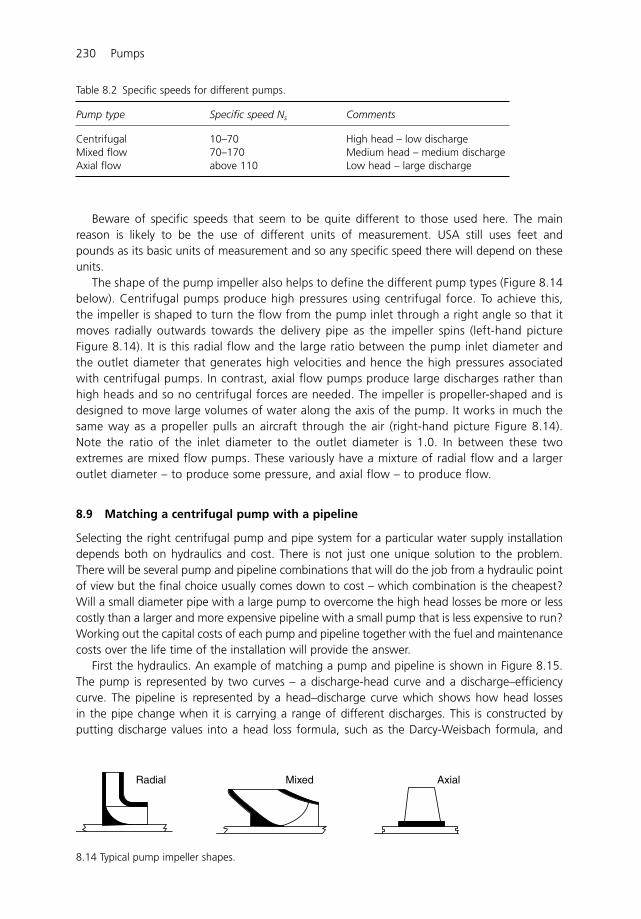
Beware of specific speeds that seem to be quite different to those used here. The mainreason is likely to be the use of different units of measurement. USA still uses feet andpounds as its basic units of measurement and so any specific speed there will depend on theseunits.
The shape of the pump impeller also helps to define the different pump types (Figure 8.14below). Centrifugal pumps produce high pressures using centrifugal force. To achieve this,the impeller is shaped to turn the flow from the pump inlet through a right angle so that itmoves radially outwards towards the delivery pipe as the impeller spins (left-hand pictureFigure 8.14). It is this radial flow and the large ratio between the pump inlet diameter andthe outlet diameter that generates high velocities and hence the high pressures associatedwith centrifugal pumps. In contrast, axial flow pumps produce large discharges rather thanhigh heads and so no centrifugal forces are needed. The impeller is propeller-shaped and isdesigned to move large volumes of water along the axis of the pump. It works in much thesame way as a propeller pulls an aircraft through the air (right-hand picture Figure 8.14).Note the ratio of the inlet diameter to the outlet diameter is 1.0. In between these twoextremes are mixed flow pumps. These variously have a mixture of radial flow and a largeroutlet diameter – to produce some pressure, and axial flow – to produce flow.
8.9 Matching a centrifugal pump with a pipeline
Selecting the right centrifugal pump and pipe system for a particular water supply installationdepends both on hydraulics and cost. There is not just one unique solution to the problem.There will be several pump and pipeline combinations that will do the job from a hydraulic pointof view but the final choice usually comes down to cost – which combination is the cheapest?Will a small diameter pipe with a large pump to overcome the high head losses be more or lesscostly than a larger and more expensive pipeline with a small pump that is less expensive to run?Working out the capital costs of each pump and pipeline together with the fuel and maintenancecosts over the life time of the installation will provide the answer.
First the hydraulics. An example of matching a pump and pipeline is shown in Figure 8.15.The pump is represented by two curves – a discharge-head curve and a discharge–efficiencycurve. The pipeline is represented by a head–discharge curve which shows how head lossesin the pipe change when it is carrying a range of different discharges. This is constructed byputting discharge values into a head loss formula, such as the Darcy-Weisbach formula, and
230 Pumps
Table 8.2 Specific speeds for different pumps.
Pump type Specific speed Ns Comments
Centrifugal 10–70 High head – low dischargeMixed flow 70–170 Medium head – medium dischargeAxial flow above 110 Low head – large discharge
Radial Mixed Axial
8.14 Typical pump impeller shapes.
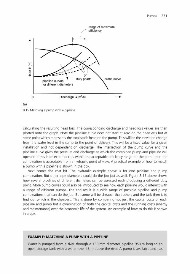
Pumps 231
8.15 Matching a pump with a pipeline.
calculating the resulting head loss. The corresponding discharge and head loss values are thenplotted onto the graph. Note the pipeline curve does not start at zero on the head axis but atsome point which represents the total static head on the pump. This will be the elevation changefrom the water level in the sump to the point of delivery. This will be a fixed value for a giveninstallation and not dependent on discharge. The intersection of the pump curve and thepipeline curve gives the pressure and discharge at which the combined pump and pipeline willoperate. If this intersection occurs within the acceptable efficiency range for the pump then thecombination is acceptable from a hydraulic point of view. A practical example of how to matcha pump with a pipeline is shown in the box.
Next comes the cost bit. The hydraulic example above is for one pipeline and pumpcombination. But other pipe diameters could do the job just as well. Figure 8.15 above showshow several pipelines of different diameters can be assessed each producing a different dutypoint. More pump curves could also be introduced to see how each pipeline would interact witha range of different pumps. The end result is a wide range of possible pipeline and pumpcombinations that can do the job. But some will be cheaper than others and the task then is tofind out which is the cheapest. This is done by comparing not just the capital costs of eachpipeline and pump but a combination of both the capital costs and the running costs (energyand maintenance) over the economic life of the system. An example of how to do this is shownin a box.
EXAMPLE: MATCHING A PUMP WITH A PIPELINE
Water is pumped from a river through a 150 mm diameter pipeline 950 m long to anopen storage tank with a water level 45 m above the river. A pump is available and has
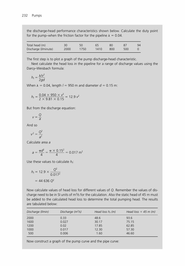
the discharge-head performance characteristics shown below. Calculate the duty pointfor the pump–when the friction factor for the pipeline � � 0.04.
Total head (m) 30 50 65 80 87 94Discharge (l/minute) 2000 1750 1410 800 500 0
The first step is to plot a graph of the pump discharge-head characteristic.Next calculate the head loss in the pipeline for a range of discharge values using the
Darcy–Weisbach formula:
When � � 0.04, length l � 950 m and diameter d � 0.15 m:
But from the discharge equation:
And so
Calculate area a
Use these values to calculate hf:
� 44 636 Q2
Now calculate values of head loss for different values of Q. Remember the values of dis-charge need to be in SI units of m3/s for the calculation. Also the static head of 45 m mustbe added to the calculated head loss to determine the total pumping head. The resultsare tabulated below:
Discharge (l/min) Discharge (m3/s) Head loss hf (m) Head loss � 45 m (m)
2000 0.33 48.6 93.61600 0.027 30.17 75.151200 0.02 17.85 62.851000 0.017 12.30 57.30500 0.006 1.60 46.60
Now construct a graph of the pump curve and the pipe curve:
hf � 12.9 � Q2
0.0172
a � �d2
4 � � � 0.152
4 � 0.017 m2
v 2 � Q2
a2
v � Qa
� 0.04 � 950 � v2
2 � 9.81 � 0.15 � 12.9 v2hf
hf � �/v2
2gd
232 Pumps
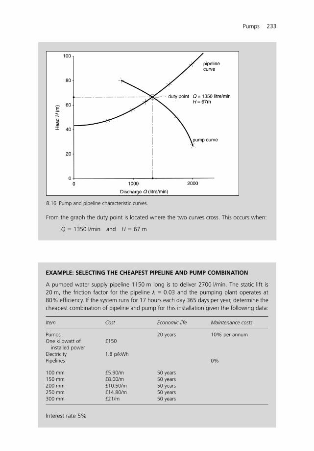
Pumps 233
From the graph the duty point is located where the two curves cross. This occurs when:
Q � 1350 l/min and H � 67 m
EXAMPLE: SELECTING THE CHEAPEST PIPELINE AND PUMP COMBINATION
A pumped water supply pipeline 1150 m long is to deliver 2700 l/min. The static lift is20 m, the friction factor for the pipeline � � 0.03 and the pumping plant operates at80% efficiency. If the system runs for 17 hours each day 365 days per year, determine thecheapest combination of pipeline and pump for this installation given the following data:
Item Cost Economic life Maintenance costs
Pumps 20 years 10% per annumOne kilowatt of £150
installed powerElectricity 1.8 p/kWhPipelines 0%
100 mm £5.90/m 50 years150 mm £8.00/m 50 years200 mm £10.50/m 50 years250 mm £14.80/m 50 years300 mm £21/m 50 years
Interest rate 5%
8.16 Pump and pipeline characteristic curves.
234 Pumps
To calculate the cost of pumping first determine the power requirement of each pipe-pump combination. So use the power formula:
power (kW) � discharge (m3/h) � head (m)367 � efficiency
We know the discharge is 2700 l/min (162 m3/h) and the efficiency is 80% (0.8 in theformula) but we do not know the head which is a combination of the static head and thehead loss in the pipeline. So first calculate the head loss hf using the Darcy–Weisbachformula:
To calculate velocity use the discharge equation:
Calculate area a:
Put this into the equation for v:
Now calculate the power for each of the pipe and pump combinations. The results aretabulated below.
Pipe dia Velocity Head loss Static head Total pumping Power (kW)(mm) (m/s) (m) head (m)
100 5.73 577.84 20 597.84 329.89150 2.55 76.09 20 96.09 53.03200 1.43 18.06 20 38.06 21.00250 0.92 5.92 20 25.92 14.30300 0.64 2.38 20 22.38 12.35
In order to combine and compare capital costs and operating costs of the various pipeline-pump combinations calculate the equivalent annual costs for each system (if you are notfamiliar with discounting cash flows then please refer to any basic economics text book).First calculate the annual pump cost:
annual pump cost (£) � energy cost � annual replacement cost� maintenance cost � annual interest cost
Calculate each component of the annual pump cost:
energy cost (£) � operating time (h) � power (kW) � cost (£/kWh)� 17 � 365 � power (kW) � cost (£/kWh)� 6205 � power (kW) � cost (£/kWh)
v � 4Q
�d 2
a � �d 2
4
v � Qa
hf � �/v2
2gd
Pumps 235
The pump must be replaced every 20 years so the annual replacement cost is 5% of thecapital cost of the pump.
annual replacement cost � % annual replacement � capital cost (£)� 0.05 � £150 � installed power (kW)
maintenance cost � 10% of capital cost� 0.1 � £150 � installed power (kW)
annual interest cost � pump capital cost (£) � interest rate (%)� £150 � installed power (kW) � interest rate (%)
Add all these costs together for each pump to obtain the annual cost of pumping:
Pipe dia Capital cost Energy cost Replacement Maintenance Interest cost Total annual(mm) (£) (£) cost (£) cost (£) (£) cost (£)(1) (2) (3) (4) (5) (6) (3)�(4)�
(5)�(6)
100 49 484 36 845 2474 4948 2474 46 741150 7953 5922 397 795 397 7511200 3150 2345 157 315 157 2974250 2145 1597 107 214 107 2025300 1852 1379 92 185 92 1748
Now calculate the annual cost of each pipeline over the economic life of the pipeline (notein this instance there is no maintenance cost):
annual pipe cost (£) � annual replacement cost � annual interest cost
Calculate each component of the annual pipeline cost:
The pipe must be replaced every 50 years so the annual replacement cost is 2% of thecapital cost of the pipe.
annual replacement cost � % annual replacement � capital cost (£)� 0.02 � capital cost (£)
annual interest cost � capital cost (£) � interest rate (%)
Add all these together to determine the annual cost of the pipelines:
Pipe dia (mm) Capital cost (£) Replacement cost (£) Interest cost (£) Total annual cost (£)(1) (2) (3) (2)�(3)
100 6785 135 339 474150 9200 184 460 644200 12 075 241 603 845250 17 020 340 851 1191300 24 150 483 1207 1690
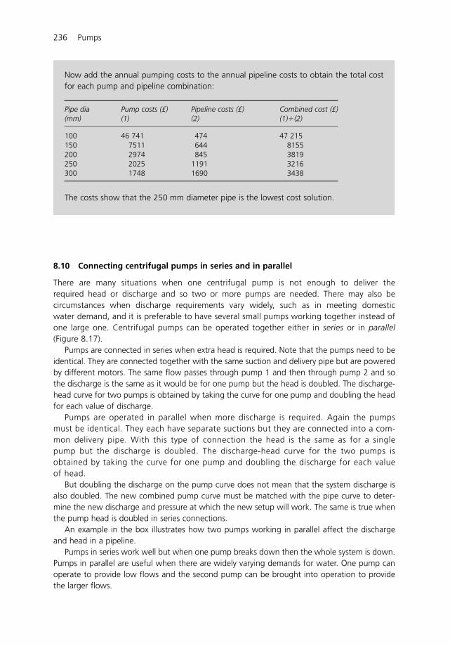
236 Pumps
Now add the annual pumping costs to the annual pipeline costs to obtain the total costfor each pump and pipeline combination:
Pipe dia Pump costs (£) Pipeline costs (£) Combined cost (£)(mm) (1) (2) (1)(2)
100 46 741 474 47 215150 7511 644 8155200 2974 845 3819250 2025 1191 3216300 1748 1690 3438
The costs show that the 250 mm diameter pipe is the lowest cost solution.
8.10 Connecting centrifugal pumps in series and in parallel
There are many situations when one centrifugal pump is not enough to deliver therequired head or discharge and so two or more pumps are needed. There may also becircumstances when discharge requirements vary widely, such as in meeting domesticwater demand, and it is preferable to have several small pumps working together instead ofone large one. Centrifugal pumps can be operated together either in series or in parallel(Figure 8.17).
Pumps are connected in series when extra head is required. Note that the pumps need to beidentical. They are connected together with the same suction and delivery pipe but are poweredby different motors. The same flow passes through pump 1 and then through pump 2 and sothe discharge is the same as it would be for one pump but the head is doubled. The discharge-head curve for two pumps is obtained by taking the curve for one pump and doubling the headfor each value of discharge.
Pumps are operated in parallel when more discharge is required. Again the pumpsmust be identical. They each have separate suctions but they are connected into a com-mon delivery pipe. With this type of connection the head is the same as for a singlepump but the discharge is doubled. The discharge-head curve for the two pumps isobtained by taking the curve for one pump and doubling the discharge for each valueof head.
But doubling the discharge on the pump curve does not mean that the system discharge isalso doubled. The new combined pump curve must be matched with the pipe curve to deter-mine the new discharge and pressure at which the new setup will work. The same is true whenthe pump head is doubled in series connections.
An example in the box illustrates how two pumps working in parallel affect the dischargeand head in a pipeline.
Pumps in series work well but when one pump breaks down then the whole system is down.Pumps in parallel are useful when there are widely varying demands for water. One pump canoperate to provide low flows and the second pump can be brought into operation to providethe larger flows.
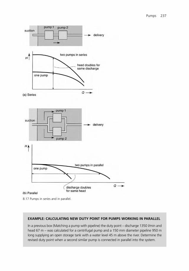
Pumps 237
8.17 Pumps in series and in parallel.
EXAMPLE: CALCULATING NEW DUTY POINT FOR PUMPS WORKING IN PARALLEL
In a previous box (Matching a pump with pipeline) the duty point – discharge 1350 l/min andhead 67 m – was calculated for a centrifugal pump and a 150 mm diameter pipeline 950 mlong supplying an open storage tank with a water level 45 m above the river. Determine therevised duty point when a second similar pump is connected in parallel into the system.
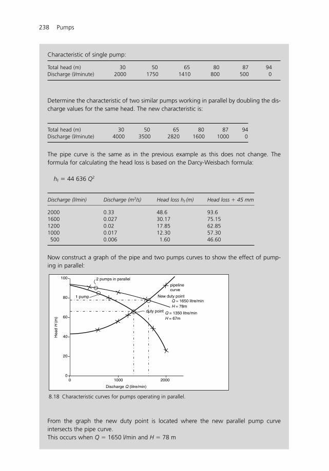
238 Pumps
Characteristic of single pump:
Total head (m) 30 50 65 80 87 94Discharge (l/minute) 2000 1750 1410 800 500 0
Determine the characteristic of two similar pumps working in parallel by doubling the dis-charge values for the same head. The new characteristic is:
Total head (m) 30 50 65 80 87 94Discharge (l/minute) 4000 3500 2820 1600 1000 0
The pipe curve is the same as in the previous example as this does not change. Theformula for calculating the head loss is based on the Darcy-Weisbach formula:
hf � 44 636 Q2
Discharge (l/min) Discharge (m3/s) Head loss hf (m) Head loss � 45 mm
2000 0.33 48.6 93.61600 0.027 30.17 75.151200 0.02 17.85 62.851000 0.017 12.30 57.30500 0.006 1.60 46.60
Now construct a graph of the pipe and two pumps curves to show the effect of pump-ing in parallel:
From the graph the new duty point is located where the new parallel pump curveintersects the pipe curve.This occurs when Q � 1650 l/min and H � 78 m
100
80
60
40
20
1000
Discharge Q (litre/min)
duty point
2 pumps in parallel
1 pump
Hea
d H
(m
)
2000
Q = 1350 litre/minH = 67m
pipelinecurve
New duty pointQ = 1650 litre/minH = 78m
00
8.18 Characteristic curves for pumps operating in parallel.

Pumps 239
8.11 Variable speed pumps
Centrifugal pump installations are designed to the meet the maximum discharge at a particularrunning speed. Lower discharges are then dealt with by throttling the flow using various typesof valve installed along the pipeline. This works fine as a control mechanism but the pump is stillusing up energy as if it was delivering the design discharge and so a lot of energy is wasted. Atypical electric motor costing some £500 could consume over £50 000 in electricity charges overits useful life and so a single percentage point increase in efficiency can save as much as thecapital cost of the motor itself.
One solution to the varying flow problem is to vary the pump speed to fit with the changein demand. But this is not always convenient and easy to do. Electric motors, which are increas-ingly used to drive pumps, are usually ac induction motors and they run at a fixed speed whichis determined by the frequency of the alternating electricity supply. In the UK this is 50 Hz (50cycles per second) so motors (and pumps) run at 3000 rpm. In some countries the ac supply is60 Hz and so motors there run at 3600 rpm.
It is possible to vary motor speed by setting a number of predetermined speeds using differentmotor wiring systems. But another way is to vary the frequency of the electricity supply. This isa recent innovation for controlling pumps. The pump motor is fitted with a frequency converterand various electronic sensors so that the pump can be set to run at a constant pressure over awide range of discharges or at a constant discharge over a wide range of pressures (Figure 8.19).They are often referred to as inverters but this describes only part of their function. The fre-quency converter adjusts the motor and hence the pump speed so that the various set demandsare met. This can significantly reduce energy demands and the costs of pumping.
8.12 Operating pumps
Here are some good practical guidelines for operating pumps properly.
8.12.1 Centrifugal pumps
Centrifugal pumps always have control valves fitted on the suction and delivery sides of thepump. The valve on the delivery side is used to control pressure and discharge (Figure 8.8). It isclosed before starting so that the pump can be primed. Once the pump is running it is slowlyopened to deliver the flow.
A reflux (non-return) valve is also usually fitted after the delivery valve to stop reverse flows thatcan damage the pump (Section 8.14). Some reflux valves have a small by-pass valve fitted whichallows water stored in the pipe to pass around the valve and be used for priming the pump.
A reflux valve is usually fitted on the end of the suction pipe. This keeps the suction pipe fullof water and makes priming easier.
Before starting a pump, the delivery valve must be closed. The pump and the suction pipeare then filled with water for priming. When pumps are located below the sump water level theyare primed automatically as water flows under gravity into the pump casing. Contrary to expec-tation starting a pump with a closed delivery valve does not cause problems. The pressure doesnot go on rising and damage the pump. Rather it reaches a steady speed and pressure.Remember the pressure depends only on the speed of rotation of the impeller. The faster itrotates the higher will be the pressure. The delivery valve is then slowly opened, water flows intothe pipeline and as the discharge increases the pressure at the pump gradually falls. At the sametime the power requirement increases. This gradual change continues until the delivery pipe isfull of water and the system is operating at its design head and discharge.
These operating procedures are important for several reasons. Suppose for example, thedelivery valve was left open as often happens. Not only would it be difficult to prime the pump
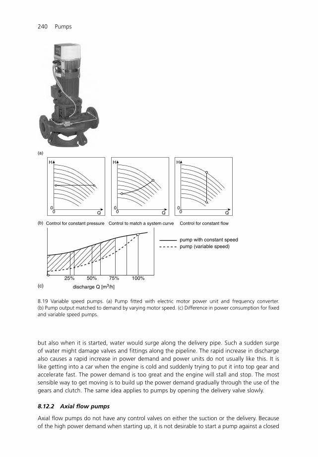
240 Pumps
(a)
Control for constant pressure(b) Control to match a system curve Control for constant flow
QQQ
HHH
00
00
00
discharge Q [m3/h]
pump with constant speedpump (variable speed)
100%75%50%25%
(c)
8.19 Variable speed pumps. (a) Pump fitted with electric motor power unit and frequency converter. (b) Pump output matched to demand by varying motor speed. (c) Difference in power consumption for fixedand variable speed pumps.
but also when it is started, water would surge along the delivery pipe. Such a sudden surgeof water might damage valves and fittings along the pipeline. The rapid increase in dischargealso causes a rapid increase in power demand and power units do not usually like this. It islike getting into a car when the engine is cold and suddenly trying to put it into top gear andaccelerate fast. The power demand is too great and the engine will stall and stop. The mostsensible way to get moving is to build up the power demand gradually through the use of thegears and clutch. The same idea applies to pumps by opening the delivery valve slowly.
8.12.2 Axial flow pumps
Axial flow pumps do not have any control valves on either the suction or the delivery. Becauseof the high power demand when starting up, it is not desirable to start a pump against a closed
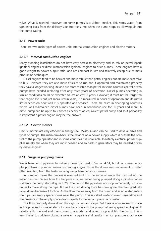
valve. What is needed, however, on some pumps is a siphon breaker. This stops water fromsiphoning back from the delivery side into the sump when the pump stops by allowing air intothe pump casing.
8.13 Power units
There are two main types of power unit: internal combustion engines and electric motors.
8.13.1 Internal combustion engines
Many pumping installations do not have easy access to electricity and so rely on petrol (sparkignition) engines or diesel (compression ignition) engines to drive pumps. These engines have agood weight to power output ratio, and are compact in size and relatively cheap due to massproduction techniques.
Diesel engines tend to be heavier and more robust than petrol engines but are more expensiveto buy. However, they are also more efficient to run and if operated and maintained properlythey have a longer working life and are more reliable than petrol. In some countries petrol-drivenpumps have needed replacing after only three years of operation. Diesel pumps operating insimilar conditions could be expected to last at least 6 years. However, it must not be forgottenthat engine life is not just measured in years, it is measured in hours of operation and its usefullife depends on how well it is operated and serviced. There are cases in developing countrieswhere well maintained diesel pumps have been in continuous use for 30 years and more. Adiesel pump can be up to four times as heavy as an equivalent petrol pump and so if portabilityis important a petrol engine may be the answer.
8.13.2 Electric motors
Electric motors are very efficient in energy use (75–85%) and can be used to drive all sizes andtypes of pumps. The main drawback is the reliance on a power supply which is outside the con-trol of the pump operator and in some countries it is unreliable. Inevitably electrical power sup-plies usually fail when they are most needed and so backup generators may be needed drivenby diesel engines.
8.14 Surge in pumping mains
Water hammer in pipelines has already been discussed in Section 4.14, but it can cause partic-ular problems in pumping mains by creating surges. This is the slower mass movement of wateroften resulting from the faster moving water hammer shock waves.
In pumping mains the process is reversed and it is the surge of water that can set up thewater hammer. To see how this happens imagine water being pumped along a pipeline whensuddenly the pump stops (Figure 8.20). The flow in the pipe does not stop immediately but con-tinues to move along the pipe. But as the main driving force has now gone, the flow graduallyslows down because of friction. As the flow moves away from the pump and as no water entersthe pipe, an empty space forms near the pump. This is called water column separation andthe pressure in the empty space drops rapidly to the vapour pressure of water.
The flow gradually slows down through friction and stops. But there is now an empty spacein the pipe and so water starts to flow back towards the pump gathering speed as it goes. Itrapidly refills the void and then comes to a sudden and violent stop as it hits the pump. This isvery similar to suddenly closing a valve on a pipeline and results in a high pressure shock wave
Pumps 241
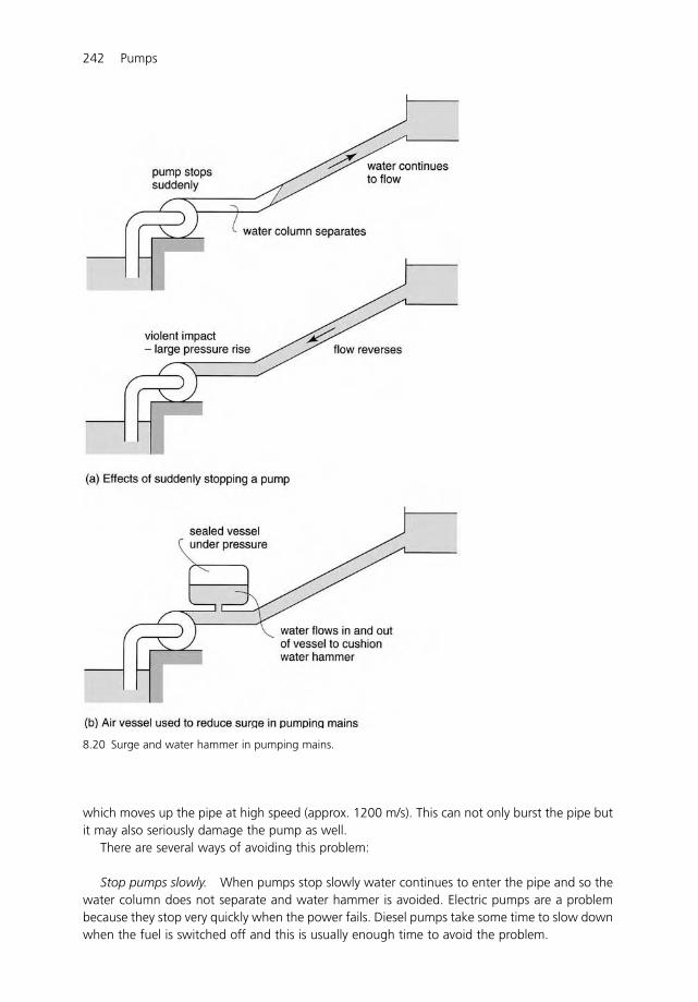
which moves up the pipe at high speed (approx. 1200 m/s). This can not only burst the pipe butit may also seriously damage the pump as well.
There are several ways of avoiding this problem:
Stop pumps slowly. When pumps stop slowly water continues to enter the pipe and so thewater column does not separate and water hammer is avoided. Electric pumps are a problembecause they stop very quickly when the power fails. Diesel pumps take some time to slow downwhen the fuel is switched off and this is usually enough time to avoid the problem.
242 Pumps
8.20 Surge and water hammer in pumping mains.
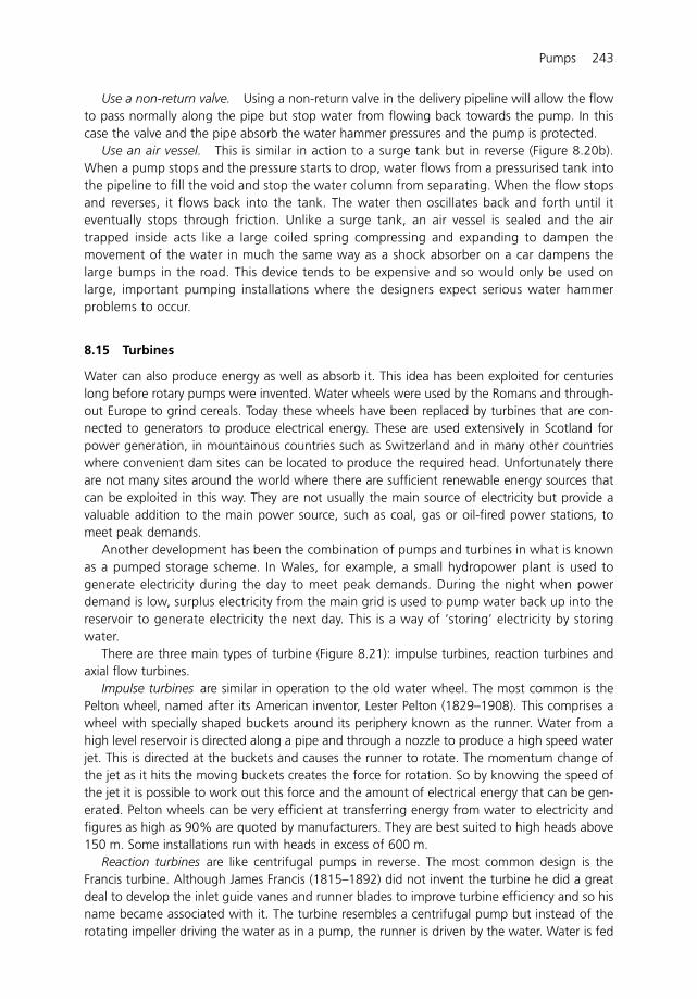
Use a non-return valve. Using a non-return valve in the delivery pipeline will allow the flowto pass normally along the pipe but stop water from flowing back towards the pump. In thiscase the valve and the pipe absorb the water hammer pressures and the pump is protected.
Use an air vessel. This is similar in action to a surge tank but in reverse (Figure 8.20b).When a pump stops and the pressure starts to drop, water flows from a pressurised tank intothe pipeline to fill the void and stop the water column from separating. When the flow stopsand reverses, it flows back into the tank. The water then oscillates back and forth until iteventually stops through friction. Unlike a surge tank, an air vessel is sealed and the airtrapped inside acts like a large coiled spring compressing and expanding to dampen themovement of the water in much the same way as a shock absorber on a car dampens thelarge bumps in the road. This device tends to be expensive and so would only be used onlarge, important pumping installations where the designers expect serious water hammerproblems to occur.
8.15 Turbines
Water can also produce energy as well as absorb it. This idea has been exploited for centurieslong before rotary pumps were invented. Water wheels were used by the Romans and through-out Europe to grind cereals. Today these wheels have been replaced by turbines that are con-nected to generators to produce electrical energy. These are used extensively in Scotland forpower generation, in mountainous countries such as Switzerland and in many other countrieswhere convenient dam sites can be located to produce the required head. Unfortunately thereare not many sites around the world where there are sufficient renewable energy sources thatcan be exploited in this way. They are not usually the main source of electricity but provide avaluable addition to the main power source, such as coal, gas or oil-fired power stations, tomeet peak demands.
Another development has been the combination of pumps and turbines in what is knownas a pumped storage scheme. In Wales, for example, a small hydropower plant is used togenerate electricity during the day to meet peak demands. During the night when powerdemand is low, surplus electricity from the main grid is used to pump water back up into thereservoir to generate electricity the next day. This is a way of ‘storing’ electricity by storingwater.
There are three main types of turbine (Figure 8.21): impulse turbines, reaction turbines andaxial flow turbines.
Impulse turbines are similar in operation to the old water wheel. The most common is thePelton wheel, named after its American inventor, Lester Pelton (1829–1908). This comprises awheel with specially shaped buckets around its periphery known as the runner. Water from ahigh level reservoir is directed along a pipe and through a nozzle to produce a high speed waterjet. This is directed at the buckets and causes the runner to rotate. The momentum change ofthe jet as it hits the moving buckets creates the force for rotation. So by knowing the speed ofthe jet it is possible to work out this force and the amount of electrical energy that can be gen-erated. Pelton wheels can be very efficient at transferring energy from water to electricity andfigures as high as 90% are quoted by manufacturers. They are best suited to high heads above150 m. Some installations run with heads in excess of 600 m.
Reaction turbines are like centrifugal pumps in reverse. The most common design is theFrancis turbine. Although James Francis (1815–1892) did not invent the turbine he did a greatdeal to develop the inlet guide vanes and runner blades to improve turbine efficiency and so hisname became associated with it. The turbine resembles a centrifugal pump but instead of therotating impeller driving the water as in a pump, the runner is driven by the water. Water is fed
Pumps 243
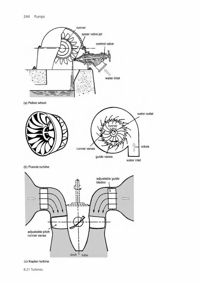
244 Pumps
8.21 Turbines.
Pumps 245
under pressure and at high velocity around a spiral casing onto the runner and as rotates thepressure and kinetic energy of the water is transferred to the runner. Francis turbines normallywork at heads of 15–150 m.
Axial flow (or propeller) turbines are known as Kaplan turbines. They are named afterVictor Kaplan (1876–1934), a German professor who developed this type of turbine withadjustable blades. Axial flow turbines operate like axial flow pumps in reverse. They operateat low heads (less than 30 m) and are used in tidal power installations. They have blades ontheir runners that can be twisted to different angles in order to work at high efficiency overa wide range of operating conditions. This kind of turbine is also used in pumped storageschemes. It is used as a turbine during the day when power demand is high and at night itis connected to an electric motor and used as a pump to lift water back into a high levelreservoir in readiness for the next day.
8.16 Some examples to test your understanding
1 A centrifugal pump is connected to a 25 m length of 300 mm diameter suction pipe anddischarges into a 500 m long pipe with a diameter of 150 mm. The water level in the riveris 2 m above datum, the centre line of the pump is 3.75 m higher, and the discharge pipeenters a tank whose water level is 25 m above datum. Calculate the pressure head that thepump must produce to pump a discharge of 0.150 m3/s. Assume a friction factor of� � 0.015 (61.8m).
2 A pump supplies water to a large reservoir through a 2000 m long pipeline 400 mm indiameter. If the difference in water level between the sump and the reservoir is 20 m andthe friction factor for the pipeline is � � 0.03, calculate the pressure and power outputrequired to deliver a discharge of 0.35 m3/s (29.38 m; 101 kW).
3 A centrifugal pump lifts water from a well to a storage tank with an outlet 20 m above thewater level in the well. The suction and delivery pipes are 50 mm in diameter and the totalpipe length is 150 m. The friction factor for the pipeline is � � 0.035. The pump perform-ance at different heads is tabulated below:
Head (m) 0 12 25 30 32 33Discharge (l/s) 9 8 6 4 2 0Efficiency (%) 0 50 60 60 50 0
Plot the pump characteristic curves and the pipe system curve and determine the discharge,head, efficiency, and power required at the duty point (2.8 l/s; 31 m; 56%; 0.85 kW).If a second pump is connected in series calculate the new duty point (4.8 l/s; 57 m; 60%;2.64 kW).
9 Bathtub hydraulics
Having a bath is a good practical way to learn about hydraulics. Here are just some of the thingsto look out for.
Just filling the bath can be an experience in itself. The hot and cold water taps are runningbut then you notice that the two are not mixing well. One side of the bath is hot and the othercold. There is some mixing at the interface due to turbulence but this is all. The only way to getan even temperature is to stir the water vigorously with your hand. The reason for this mixingproblem is that water density varies slightly with temperature and this density difference isenough to inhibit mixing. This is a major problem at most power generating stations that usevast quantities of water from rivers and the sea to cool their systems. High towers help to coolwater before it is returned to the river or sea but any slight difference in temperature will stopit mixing fully with the receiving flow. Swimming downstream of a power station can be a pleas-ant, warm experience. The challenge for the engineers is to find ways of mixing the water thor-oughly so that the receiving water returns to its original temperature as quickly as possible so asnot to affect local aquatic plant and fish life. It also stops hot water short-circuiting the systemand finding its way into the intake and back into the power station as can happen with coastalstations.
As water flows from the taps across the bottom of the bath the flow is usually super-critical –fast and shallow. But this state soon changes as a hydraulic jump forms at the far end and thenquickly makes its way back towards the tap end as a travelling surge wave (Section 6.4). For awhile a stable circular hydraulic jump can be seen just where the water plunges into the bathbut eventually this is drowned out as the level in the bath rises. The incoming flow is still super-critical and this now shoots under the slow flow. The energy is not dispersed in the hydraulicjump, it is gradually absorbed as friction along the base of the bath slows the water down.When this occurs in natural channels it can cause severe erosion of the bed and sides(Section 7.2.1).
Once your bath is full to the right level and is at the right temperature, there is now that‘Eureka moment’ that Archimedes experienced when he stepped into the water. Archimedesfirst discovered the significance of this some 2000 years ago when he realised that the waterdisplaced when you get into the bath has the same volume as your body. He also noticed thatif you float on the water instead of sitting on the bottom then the amount of water you dis-place is equal to your weight. From this he was able to solve the problem that the King ofSyracuse had over what materials had been used to make his crown – was it gold or was it really
Bathtub hydraulics 247
lead (Section 2.12)? This was the beginning of our understanding of hydrostatics (water whichis not moving) and led to formulae for the design and construction of water tanks, dams andsubmarines that we still use today. It is an almost perfect theory. It was unfortunate that theGreeks also tried their hand at hydrodynamics – water which is moving – but they got this bitwrong and sent science off in the wrong direction for almost 2000 years. We had to wait untilthe likes of Sir Isaac Newton came along to put things right.
Sitting still in a bath and soaking up the warmth is a good experience – but for children this isalmost impossible. Sliding up and down quickly is much more fun as you can make waves and evenmake the water flow over the sides of the bath. This is because water is a real fluid with viscous prop-erties. As you start to move up and down the bath you transfer your body momentum to the waterby surface and form drag (Section 3.10) – the larger you are the more form drag you can create andthe more water you can move. When you stop sliding about, the waves seem to continue for a whilebefore they stop. This is because the only force available to absorb the wave energy is friction andas there is very little of this in a bath it takes some time to suppress the waves. Water can also sloshabout in harbours in much the same way as the bath tub and it can cause lots of problems for ships.The wave energy comes from the sea, it enters the harbour and it is difficult to get rid of because,like the bathtub, the walls of the harbour reflect the energy rather than absorb it. The movement ofthe water can move ships back and forth on their moorings which can be a major problem if theship happens to be a supertanker and you are trying to keep it still while loading it with oil. This iswhy harbour entrances are narrow and specially angled to stop wave energy from entering. You mayhave noticed that the sea is much calmer inside a harbour than outside. Some harbours though havebeen known to behave in quite the opposite way. When the entrance is narrow the waves insideseem to get larger. This is a resonance effect that harbour designers must guard against.
As you relax in the bath you decide to have a drink. A glass of whisky will do the trick butyou want water with it. So here is a little puzzle to while away the time. Do you put the waterin the whisky or the whisky in the water? Start with a glass of water and a glass of whisky. Onespoonful of whisky is put into the water and mixed and then one spoonful of the mixture is putback into the whisky. Is there more whisky in the water or more water in the whisky? If youcannot work it out then have a look at the solution in the box.
It is now time to get out of your bath and take out the plug. Notice how this sets up a nicewhirlpool around the plug hole and it seems to be hollow down the middle. This is a boundarylayer effect similar to those described in Section 3.9.3. The boundary layer close to the outletslows the flow velocity which makes the water swirl and the vortex then forms. We say that theboundary layer curls up. All water intakes at reservoirs and control gates along rivers suffer fromvortices like this which draw in air and reduce the water discharge. If you put some floatingobject over the vortex, such as your plastic duck, it stops the swirling and the discharge downthe plughole increases. This is what engineers do in practice to stop vortices from forming at off-takes and also pump station suction inlets. Setting the outlet or the pump intake deep belowthe water surface will also suppress the vortices.
Finally there is the inevitable question that I am sure will keep you awake at night – whichway does the vortex go? Some say that the vortex goes in a clockwise direction in the northernhemisphere and anticlockwise in the southern hemisphere. There is a very practical demonstra-tion of this by an enterprising young man who lives on the equator in Kenya and puts ondemonstrations for the tourists. He has a large can filled with water which he sets up 20 m northof the equator. When he pulls a plug out of the bottom of the container the water slowly startsto swirl in a clockwise direction. He then does the same test 20 m south of the equator and theswirl starts in an anticlockwise direction. It works every time. Convinced? The reality is that noone is absolutely sure. Experiments to test the theory have been tried but they are very difficult
248 Bathtub hydraulics
to do in a laboratory. The problem is that the force which causes the movement – the Coriolisforce which comes from the earth’s rotation – is very small in comparison to other forces aroundsuch as minor vibrations due to traffic outside the laboratory or temperature changes in theroom setting up convection currents in the tank. All these can significantly influence which waythe water will begin to swirl and override the effects of the Coriolis force. A large tank of wateris needed to get an appreciable Coriolis force but arranging this under laboratory conditions isnot very practicable.
If you have an aversion to baths and you prefer a shower there is always something to learnhere though it may not be as much fun. When you switch on the shower and draw the plasticcurtain around you for a bit of privacy, have you noticed how it tends to cling to your body – itis cold and uncomfortable. This is because the fast downward flow of water from the showercauses a slight drop in air pressure within the curtained space (remember the energy equation –energy changes from pressure energy to kinetic energy). The pressure outside the curtain is stillat atmospheric pressure – slightly greater than the air pressure inside – and so the pressuredifference causes the curtain to move towards the water and to cling to you.
Once you start to appreciate what is going on in your bath, bath-times will never be the sameagain!
EXAMPLE: A MIXING PROBLEM
Take one glass of water and a equal glass of whisky. One spoonful of whisky is put intothe water and mixed. One spoonful of the mixture is put back into the whisky. Is theremore whisky in the water or more water in the whisky?
Start by assuming that each glass holds 10 spoonfuls – so the water glass holds 10spoonfuls of water and the whisky glass holds 10 spoonfuls of whisky. Now follow theargument below under the water and whisky headings as liquid is moved from one tothe other:
Water Whisky
10water 10whisky
One ‘spoonful’ (one part) of water is taken from the water and added to the whisky
9water 10whisky � 1water
The whisky glass now holds 11 spoonfuls of the mix. Each spoonful of the mix comprises 10 parts water and one part whisky i.e. (10whisky � 1water)/11.
Now take one spoonful of the mix and return this to the water:
9water � (10whisky � 1water)/11 10whisky � 1water – (10whisky � 1water)/119water � 1/11 water � 10/11 whisky 10whisky � 1water – 10/11 whisky – 1/11 water
9 1/11water � 10/11whisky 9 1/11whisky � 10/11water
So the result is the amount of water in the whisky is the same as the amount of whiskyin the water. So whichever way you mix your drinks it make no difference.
References and further reading
BS3680 Measurement of Liquid Flow in Open Channels. British Standards Institution, London (also ISO 7481979)(1981) Part 4A Thin Plate Weirs(1981) Part 4C FlumesPart 4E Rectangular Broad Crested WeirsThese are the standards which are the basis for the design, installation and operation of flow measur-ing structures.
Chadwick, A., Morfett, J. and Borthwick, M. (2004) Hydraulics in Civil and Environmental Engineering. 4thedition E & FN Spon, London.Similar in some ways to Webber, this is another excellent undergraduate text but its coverage ofhydraulics is much wider and includes sediment transport, river and canal engineering, coastal engi-neering and hydrology.
Chow, V.T. (1981) Open Channel Hydraulics. International Student Edition. McGraw Hill.Although an ‘old’ book it is still the bible of open channel hydraulics. It is a handbook with lots of infor-mation on all aspects of channel flow and design – it is not an elementary text.
Douglas, J.F. (1996) Solving Problems in Fluid Mechanics Parts I and II. Longman, Harlow, UK.This is a good problem-solving-oriented text. It approaches the principles of hydraulics by showing howto solve numerical problems.
Hamill, L. (2001) Understanding Hydraulics. MacMillan Press Ltd, Basingstoke, UK.This is a book written by a teacher of hydraulics who clearly has a lot of experience of teaching a dif-ficult subject. It is written in a conversational style with the student asking questions and the teacherproviding the answers. It is sympathetic to the needs of young engineers but makes no allowances forthose with limited mathematical skills.
Hydraulics Research (1990) Charts for the Hydraulic Design of Channels and Pipes. 6th Edition. ThomasTelford Ltd.An excellent and widely used book of design charts based on the Colebrook-White equation.
King, H.W. and Brater, E.F. (1996) Handbook of Hydraulics for the Solution of Hydrostatic and Fluid FlowProblems. 7th edition. McGraw Hill.Very useful for the solution of Manning’s equation for channel flow. His method is used in this text.
Portland Cement Association (1964) Handbook of Concrete Culvert Pipe Hydraulics. Chicago, IL.Very comprehensive book on culvert hydraulics and their construction. Although it is primarilysupporting concrete culverts they can be made out of other materials as well.
Rouse, H. and Ince, S. (1957) History of Hydraulics. Dover Publications, New York.A comprehensive, well-researched and very readable history of hydraulics from the early work of Greek scholars to our modern notions of fluid behaviour. Rouse is a well-known authority onhydraulics.
250 References and further reading
USBR (1974) Design of Small Dams. United States Dept of the Interior, Bureau of Reclamation.Lots of useful construction details of hydraulic structures and particularly weirs and spillways.
Vallentine, H.R. (1967) Water in the Service of Man. Penguin Books Ltd, Harmondsworth, UK.Sadly this book is now out of print but copies are still available on the internet. It is an excellent, easyto read, introduction to the fundamentals of water flow in pipes, channels and pumps as well as pro-viding a broader appreciation of water and its uses including its history. The text is very descriptive,anecdotal and entertaining in style with lots of good explanations and very little mathematics.Vallentine is clearly an engineer who knows how to communicate his ideas in a practical and interest-ing way. Penguin really ought to reprint this book.
Webber, N.B. (1971) Fluid Mechanics for Civil Engineers. Chapman Hall, London.An excellent, comprehensive undergraduate civil engineering textbook covering both basic principlesand practical applications. Now out of print but copies still available on the internet.
acceleration 2aeroplane 69, 145air valves 117air-lift pump 209air-regulated siphons 202alternate depths 151Archimedean screw pump 209Archimedes’ principle 45atmospheric pressure 30, 94, 215axial flow pumps 214
backwater curve 142Bakhmateff, Boris 150bathtub hydraulics 246Bernoulli, Daniel 57Bernoulli equation 57black-water siphons 201Blazius, Paul 90bores: in channels 176boundary layer 74; earth’s surface 76; in pipes
and channels 75Bourdon gauge 35bridge piers 165broad-crested weirs 193
canals 123capillary waves 172capital costs 231, 234carburettors 70cavitation 74, 219celerity see wavescentrifugal pumps 212channel bends 164channels 123; alternate depths 151; backwater
curve 142; bends 164; bores 176; continuity125; critical depth 156; critical point 148;design formulae 135; discharge control 196;discharge measurement 196; energy 126;energy losses 130; Froude Number 149;gradually varied flow 131, 142; hydraulic
jump 159; hydraulic radius 134; King’s method 138; lined 134; non-uniform flow 131,142; practical design 141; roughness 135;secondary flows 163; sediment transport 166;shapes 132; slope 134; specific energy 149;stilling basin 162, 198; sub-critical flow 143;super-critical flow 144; threshold of movement168; uniform flow 131; water level control198; wetted perimeter 132
Chezy, Antoine 135Chezy formula 135Colebrook, C.F. 90Colebrook–White equation 100compressibility 20continuity 53, 125; equation 53Coriolis force 77critical: depth 156; point 148, 151critical depth structures 153crump weirs 194culverts 205
Da Vinci, Leonardo 170dams: design 38Darcy, Henry 88Darcy–Weisbach equation 88density 16; currents 177; relative 17dimensionless number: Froude No. 149;
Mach No. 149; Reynolds No. 87dimensions 1discharge 53discharge control: in channels 196discharge measurement: in channels 196drag 78drop structures 199drowned flow 185, 194
Eckman Spiral 78Eddy shedding 80efficiency see pumpsEgypt 210
Index
energy 10, 55, 126; Bernoulli 57; dissipators198; equation 57; kinetic 56; measuringvelocity 61; potential 57; pressure 56; total 57
fittings for pipes 115floating objects 47fluid injectors 71flumes 194; Parshall 194; WCS 196force 3; Coriolis 77; on dams 39; drag 78;
Newton 6; on nozzles 84; on pipe bends 114;on sluice gates 42
Fortin barometer 32Francis, James 243friction 3Froude, William 149Froude Number 149, 161
Galilei, Galileo 31The Gambia 211geostrophic wind 77gradually varied flow 131, 142gravity constant 7gravity waves 172
hand-piston pumps 209Herschel, Clemens 106hydraulic: design charts 100; gradient 92; jump
159; models 125, 194; radius 134hydraulic gradient 92hydraulic structures see structureshydrodynamics 51hydrograph 177hydrostatics 21
ideal fluid 18, 58, 170impeller 212irrigation 6, 51, 71, 121, 214
Joukowsky, Nicholai 119Joukowsky equation 120joules 10
Kaplan, Victor 245King, HW 138King’s method 138
Lagrange, Joseph 173laminar flow 86; in channels 125
Mach Number 149Manning, Robert 137Manning formula 135, 137Manning’s n 137manometers 36mass 7maximum velocity 141mercury barometer 32mixed flow pumps 215momentum 12, 72
Net Positive Suction Head 220Newton 4; laws of motion 4; Sir Isaac 4Newtonian fluids 18Nikuradse, Johann 90non-uniform flow 131, 142; gradually-varied
142; rapidly-varied 142normal depth 131
open channels see channelsorifice plate 106orifices 64; contraction coefficient 65
Parshall, RL 194Parshall flumes 194Pascal, Blaise 21Pascals 21Pelton, Lester 243piezometers 35pipes 85; Colebrook-White formula 96;
Darcy-Weisbach equation 88; design charts100; fittings 115; flow problem 85; friction89; materials 114; networks 105; nominaldiameter 114; parallel 103; rough 90; smooth 90; surge 121; velocity profile 75;water hammer 118
pitot tube 63positive displacement pumps 208power 12; see also pumpspressure 21; absolute 34; atmospheric 30;
bar 33; gauge 34; head 29; measurement 34;piezometers 35
pump performance see pumpspumps 208; air-lift 209; Archimedian screw 209;
axial flow 214; cavitation 219; centrifugal 212;delivery 217; efficiency 224; energy for 220;hand-piston 209; head 218; matching withpipeline 230; mixed flow 215; operating 239;in parallel 236; performance 227; positivedisplacement 208; power for 222; power units241; pressure 215; priming 217; roto-dynamic212; selection 229; in series 236; specificspeed 229; submersible 216; suction lift 215;treadle 209; variable speed 239
quicksand 49
rapidly-varied flow 142real fluids 73Reynolds, Osborne 86Reynolds Number 87, 90, 136, 181river off-takes 165roto-dynamic pumps 212rough pipe flow 90running cost 231Russel, John Scott 173
secondary flows 163sediment transport 166sharp-crested weirs 185
252 Index
Shields, A 168shock wave 119SI units 1siphons 94, 200; air-regulated 202;
blackwater 201sluice gates: forces on 42smooth pipe flow 90specific energy 149specific gravity 17, 47speed of sound 147spillways 51, 160, 198, 200, 202stagnation point 61stilling basin 162, 198stone-skipping 83streamlining 80structures: critical depth 185; cross regulators
182; culverts 205; drop 199; flumes 185;orifice 184; sharp-crested weirs 186; siphons200; solid weirs 188; weirs 185
sub-critical flow 143submersible pumps 216suction lift 215super-critical flow 144surface tension 19surge 121; in channels 173; in pumping
mains 241swell 172
threshold of movement 168thrust blocks 114tidal power 180Torricelli, Evangelista 31, 32, 65
treadle pumps 209, 225tsunami wave 180turbines 243turbulent flow 86; in channels 125
uniform flow 131units 1; bar 33; cgs 1; fps 1
valves: air 117; butterfly 117; discharge control118; pressure control 118; sluice 115
vectors 8velocity 2; measuring 61; profile 75; terminal 78venturi meter 106viscosity 18; kinematic 19
water: properties of 16water hammer 118water level control: in channels 198waves 170; amplitude 171; capillary 172; celerity
171; in channels 173; density currents 177;flood 176; frequency 171; gravity 172; in harbours 178; height 171; internal 178;surges 173; swell 172; tsunami 180
weight 7weirs 185; broad-crested 193; crump 194;
drowned flow 194; rectangular 186; sharp-crested 186; solid 188; Vee-notch 186
Weisbach, Julius 88wetted perimeter 132White, C.M. 90work 10WSC flumes 196
Index 253