POWER SYSTEM TRANSIENT STABILITY ANALYSIS OF STIFF SYSTEMS USING THE MULTIRATE METHOD

BY

ALEXANDER M. WESTENDORF

THESIS

Submitted in partial fulfillment of the requirements for the degree of Master of Science in Electrical and Computer Engineering

in the Graduate College of the University of Illinois at Urbana-Champaign, 2011

Urbana, Illinois

Adviser:

Professor Thomas J. Overbye

ii

ABSTRACT

Power system transient stability studies are complex and can take a substantial amount of

time to simulate. The Multirate integration method is one way to speed up simulation studies.

This thesis studies the effects of using a type of Multirate simulation method in a software

package. In this study, the Multirate method is used mainly on simulating fast transients

resulting from excitation models. Proper subinterval values to maintain stability in PowerWorld

Simulator are established for exciter eigenvalue ranges. Subintervals are applied to exciter

models of a 16,386 bus system based on exciter eigenvalues. Application of the Multirate

method on exciters provides a time savings for each time step, with the largest being a 10 percent

faster solution when using a one cycle per second time step.

iii

ACKNOWLEDGMENTS

The author would like to acknowledge Professor Thomas Overbye for his support,

patience, and advice in the completion of this thesis. He would like to thank the Department of

Electrical and Computer Engineering (ECE) and the Power and Energy Systems group in ECE

for their support and opportunities provided during his studies. Also he would like to thank his

family for its complete support throughout his studies at the University of Illinois.

iv

TABLE OF CONTENTS

CHAPTER 1: INTRODUCTION ....................................................................................................1

CHAPTER 2: NUMERICAL INTEGRATION METHODS ..........................................................6

CHAPTER 3: METHODOLOGY .................................................................................................13

CHAPTER 4: SYSTEMS OF STUDY ..........................................................................................17

CHAPTER 5: DISCUSSION OF RESULTS ................................................................................20

REFERENCES ..............................................................................................................................28

APPENDIX A: MODEL BLOCK DIAGRAMS ...........................................................................30

1

CHAPTER 1 INTRODUCTION

Modern power system dynamics require the use of computer simulation to ensure correct

operation and planning. The simulation of the system in time domain provides critical insight

into the security of the overall power system. This insight allows operators to limit the extent of

system cascading failures and improve the overall reliability. As modern systems become more

and more complicated with the introduction of FACTS device models, dynamic loads, and other

power electronic models, the system becomes more susceptible to numerical instability.

Many different numerical methods exist to solve power system dynamic equations in [1].

The basic methods for numerical analysis of transient stability problems are divided into two

main categories, implicit and explicit methods. These methods form the basis of computing

transient stability response of a system. Each family of methods realizes its own advantages and

pitfalls in regards to stability and reliability calculations. The strengths and weaknesses of each

method change with the size and type of system in question. The main concern with each

integration method is the size of the time step necessary for a numerically stable simulation.

When considering large systems of differential equations, computational savings

becomes a key focus. The step size required for a stable simulation is a determining factor in the

simulation speed. Faster simulations allow for prompt analysis of a system and any problems

that arise from an event. With sufficiently fast simulations, real-time transient stability analysis

can be performed by a system operator. A quicker reaction by the operator to any type of major

event can limit or even prevent a major cascading failure in the network [2].

Typically, power systems incur a wide range of transients throughout the models. Fast

transients are most often only a small fraction of the observed dynamics. Work has been done to

combine the short and long term analysis into one method [3]. An integration method that solves

these fast dynamics with a smaller time step than the slow transients will provide a more efficient

2

and sufficiently accurate simulation result. The Multirate method, introduced in [4], provides an

integration technique suitable for systems exhibiting a wide variety of time responses.

The Multirate method was first applied to solve power system dynamic equations in [5].

Later this method was improved to include the power system analysis of FACTS devices as well

[6]. For the Multirate method to be effective, the system must have a vast difference between the

fast and slow transients. In order to use the Multirate method effectively, a partition scheme is

developed in [7]. The error analysis of the Multirate method is considered in [8]. The Multirate

method will be considered in more detail in Chapter 2.

Multirate simulation provides a promising integration method for large power studies.

This thesis looks to analyze transient stability of power systems while focusing on integration

methods. The goal of the thesis is to provide insight into the Multirate method and its uses in a

power system simulation. The effects of using a type of Multirate method implemented in

PowerWorld Simulator are explored. The results of Multirate implementation on exciters will be

discussed in Chapter 5.

1.1 General Transient Problem

In power system stability analysis, many studies must be performed. Many stability

analysis programs use simple step-by-step integration methods to solve dynamic models. While

these methods have been around for a long time, they can still be applied to varieties of models.

They are well known and understood by the system operators. This allows easy analysis of the

simulation in practice. These methods also contain all the information necessary for the state

variables in the system. The basis of many stability studies is how the system will respond to a

major event disturbance. Multiple contingency situations may be studied such as variations of

system faults. These faults can be modeled at different locations in the system to find the effect

3

on the system. Stability studies are useful in the planning and operation of the system under the

conditions specified.

Power system equations exhibit nonlinear qualities, which become more vexing as the

system becomes larger. The equations also include a dynamic behavior in the system itself to

further complicate the solution process, necessitating basic algorithms for computer simulation.

The overall system model contains set of differential equations as described in [1]

and a set of algebraic equations

In set (1.1), each machine in the system is represented with its differential equation. A

machine’s subset of equations is uncoupled from the other machines in the network. These

equations include any dynamically modeled components and the internal dynamics of the

generators and their respective control systems. In set (1.2), the stator equations for each

machine are represented. Also included in set (1.2) are the equations describing the transmission

network.

Equation (1.1) has a specific form associated with it. This form is semi-nonlinear and is shown

in (3).

�� � ���, �� � ∙ � � � ∙ � (1.3)

The matrix A is a sparse, block diagonal, square matrix. B is rectangular, sparse, and block. If

saturation is not modeled, both A and B remain constant [1].

The algebraic set is divided into the sparse bus admittance matrix, (1.4), and forcing

function (1.5).

��, �� � � ∙ � (1.4)

�� � ���, �� (1.1)

0 � ���, �� (1.2)

4

� � ���, �� (1.5)

The vector contains the bus current injections of the network. The injections are a function of

the bus voltage, and the stator internal and terminal voltage in the network reference frame for a

load and generator, respectively. The equation (1.5) is solved and inserted into (1.3) [1].

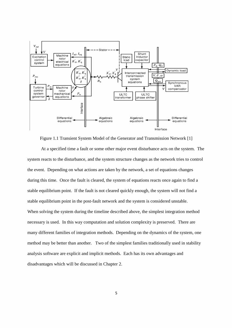
Figure 1.1 depicts the model of the machines and how they are connected to the network. It is a

representation of the aggregated power system components and the shows how they interact with

each other. More components can be added to the drawing as they are added to the system

model.

Interfacing the equations between the state equations and the dynamic equations becomes

a necessary task. For interfacing to happen, equations must share the same reference frame. The

classical machine model equations and their transformation into the industry standard reference

frame are detailed in [9] and [10]. Once all the model equations share the same reference frame,

interfacing of the equations becomes possible with interactions between different models shown

in Figure 1.1.

Typically a stability analysis is an initial value problem of the equations (1.1) and (1.2).

The solution is found through the use of a numerical integration method of choice. In a stability

study, the network achieves different states at different times. Initially the system is in steady

state equilibrium. This initialization process becomes an important step to ensure stability. If an

initial operating point of a machine is not obtained correctly, the integration method may not

converge to a proper value [1]. A discussion of the calculation of initial conditions appears in

the appendix of [1].

5

Figure 1.1 Transient System Model of the Generator and Transmission Network [1]

At a specified time a fault or some other major event disturbance acts on the system. The

system reacts to the disturbance, and the system structure changes as the network tries to control

the event. Depending on what actions are taken by the network, a set of equations changes

during this time. Once the fault is cleared, the system of equations reacts once again to find a

stable equilibrium point. If the fault is not cleared quickly enough, the system will not find a

stable equilibrium point in the post-fault network and the system is considered unstable.

When solving the system during the timeline described above, the simplest integration method

necessary is used. In this way computation and solution complexity is preserved. There are

many different families of integration methods. Depending on the dynamics of the system, one

method may be better than another. Two of the simplest families traditionally used in stability

analysis software are explicit and implicit methods. Each has its own advantages and

disadvantages which will be discussed in Chapter 2.

6

CHAPTER 2 NUMERICAL INTEGRATION METHODS

2.1 Explicit Methods

Explicit methods are used in most power system software packages. These integration

methods are easy to implement; however, there are many issues with numerical stability of the

solution method. Stiff systems create numerical stability of explicit methods. This stability

occurs when there is a large difference between the eigenvalues of the Jacobian matrix of a

system. This difference reflects a part of the system that reacts faster to a disturbance than other

areas of the system.

When determining the stability of the numerical integration scheme, the two error terms

are considered. The truncation error concerns the error that occurs from the discrete

approximation in the algorithm. Round-off error arises from the limitations of the finite word

length of the computer. For the algorithm to be considered numerically stable, the total local

error must be decreasing [11].

2.1.1 Euler

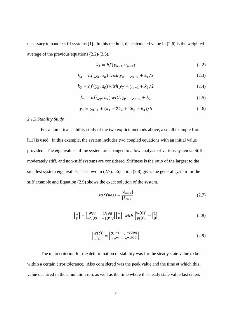
The explicit Euler method is the least complex and least accurate solution method. The

entire algorithm is shown in equation (2.1).

�� � ���� � ������ (2.1)

This method requires a very small step size on anything but the simplest of models. This method

typically takes a long time to converge due to its trivial implementation [1].

2.1.2 Runge-Kutta

The Runge-Kutta algorithm is displayed below in equations (2.2)-(2.6). This method is

discussed in detail by Dandeno and Kundur [12]. There are many different variations of this

method. One can use as many orders as they deem necessary. Typically a fourth-order is

7

necessary to handle stiff systems [1]. In this method, the calculated value in (2.6) is the weighted

average of the previous equations (2.2)-(2.5).

�� � �������, ����� (2.2)

�� � ����� , ��������� � ���� � �� 2⁄ (2.3)

�! � ����" , �"������" � ���� � �� 2⁄ (2.4)

�# � ����$ , �$������$ � ���� � �! (2.5)

�� � ���� � ��� � 2�� � 2�! � �#�/6 (2.6)

2.1.3 Stability Study

For a numerical stability study of the two explicit methods above, a small example from

[11] is used. In this example, the system includes two coupled equations with an initial value

provided. The eigenvalues of the system are changed to allow analysis of various systems. Stiff,

moderately stiff, and non-stiff systems are considered. Stiffness is the ratio of the largest to the

smallest system eigenvalues, as shown in (2.7). Equation (2.8) gives the general system for the

stiff example and Equation (2.9) shows the exact solution of the system.

'����()'' � |+,-.||+,/�| (2.7)

0��1� 2 � 0 998 19986999 619992 0�12 ���� 7��0�1�0�8 � 0102 (2.8)

7����1���8 � 72)�9 6 )��:::96)�9 6 )��:::98 (2.9)

The main criterion for the determination of stability was for the steady state value to be

within a certain error tolerance. Also considered was the peak value and the time at which this

value occurred in the simulation run, as well as the time where the steady state value last enters

8

the range of error tolerance. Different time steps were considered to determine the accuracy and

stability of the method as well.

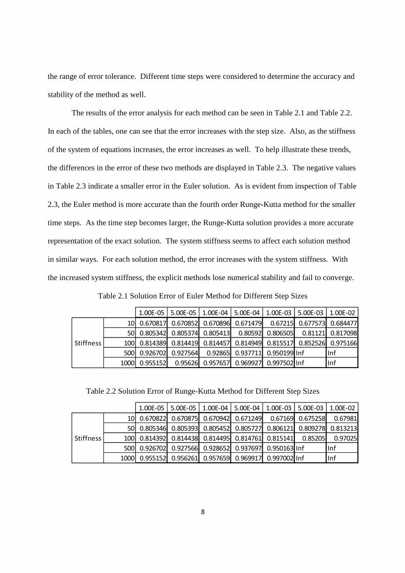
The results of the error analysis for each method can be seen in Table 2.1 and Table 2.2.

In each of the tables, one can see that the error increases with the step size. Also, as the stiffness

of the system of equations increases, the error increases as well. To help illustrate these trends,

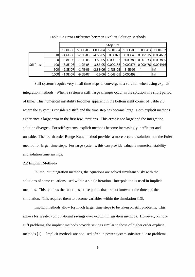
the differences in the error of these two methods are displayed in Table 2.3. The negative values

in Table 2.3 indicate a smaller error in the Euler solution. As is evident from inspection of Table

2.3, the Euler method is more accurate than the fourth order Runge-Kutta method for the smaller

time steps. As the time step becomes larger, the Runge-Kutta solution provides a more accurate

representation of the exact solution. The system stiffness seems to affect each solution method

in similar ways. For each solution method, the error increases with the system stiffness. With

the increased system stiffness, the explicit methods lose numerical stability and fail to converge.

Table 2.1 Solution Error of Euler Method for Different Step Sizes

1.00E-05 5.00E-05 1.00E-04 5.00E-04 1.00E-03 5.00E-03 1.00E-02

10 0.670817 0.670852 0.670896 0.671479 0.67215 0.677573 0.684477

50 0.805342 0.805374 0.805413 0.80592 0.806505 0.81121 0.817098

100 0.814389 0.814419 0.814457 0.814949 0.815517 0.852526 0.975166

500 0.926702 0.927564 0.92865 0.937711 0.950199 Inf Inf

1000 0.955152 0.95626 0.957657 0.969927 0.997502 Inf Inf

Stiffness

Table 2.2 Solution Error of Runge-Kutta Method for Different Step Sizes

1.00E-05 5.00E-05 1.00E-04 5.00E-04 1.00E-03 5.00E-03 1.00E-02

10 0.670822 0.670875 0.670942 0.671249 0.67169 0.675258 0.67981

50 0.805346 0.805393 0.805452 0.805727 0.806121 0.809278 0.813213

100 0.814392 0.814438 0.814495 0.814761 0.815141 0.85205 0.97025

500 0.926702 0.927566 0.928652 0.937697 0.950163 Inf Inf

1000 0.955152 0.956261 0.957659 0.969917 0.997002 Inf Inf

Stiffness

9

Table 2.3 Error Difference between Explicit Solution Methods

1.00E-05 5.00E-05 1.00E-04 5.00E-04 1.00E-03 5.00E-03 1.00E-02

10 -4.6E-06 -2.3E-05 -4.6E-05 0.00023 0.00046 0.002315 0.004667

50 -3.8E-06 -1.9E-05 -3.8E-05 0.000192 0.000385 0.001933 0.003885

100 -3.8E-06 -1.9E-05 -3.8E-05 0.000188 0.000376 0.000476 0.004916

500 -2.8E-07 -1.4E-06 -2.8E-06 1.43E-05 3.6E-05 Inf Inf

1000 -1.9E-07 -9.6E-07 -2E-06 1.04E-05 0.000499 Inf Inf

Stiffness

Step Size

Stiff systems require very small time steps to converge to a solution when using explicit

integration methods. When a system is stiff, large changes occur in the solution in a short period

of time. This numerical instability becomes apparent in the bottom right corner of Table 2.3,

where the system is considered stiff, and the time step has become large. Both explicit methods

experience a large error in the first few iterations. This error is too large and the integration

solution diverges. For stiff systems, explicit methods become increasingly inefficient and

unstable. The fourth order Runge-Kutta method provides a more accurate solution than the Euler

method for larger time steps. For large systems, this can provide valuable numerical stability

and solution time savings.

2.2 Implicit Methods

In implicit integration methods, the equations are solved simultaneously with the

solutions of some equations used within a single iteration. Interpolation is used in implicit

methods. This requires the functions to use points that are not known at the time t of the

simulation. This requires them to become variables within the simulation [13].

Implicit methods allow for much larger time steps to be taken on stiff problems. This

allows for greater computational savings over explicit integration methods. However, on non-

stiff problems, the implicit methods provide savings similar to those of higher order explicit

methods [1]. Implicit methods are not used often in power system software due to problems

10

associated with limits. When saturation limits are modeled into the system, the matrices A and B

of (1.3) have nonlinearities introduced into them. This prevents the method from having a direct

solution and convergence is questionable [1]. Many times the saturation limits are ignored with

implicit methods, thus creating some inaccuracies in the solution.

2.3 Multirate Method

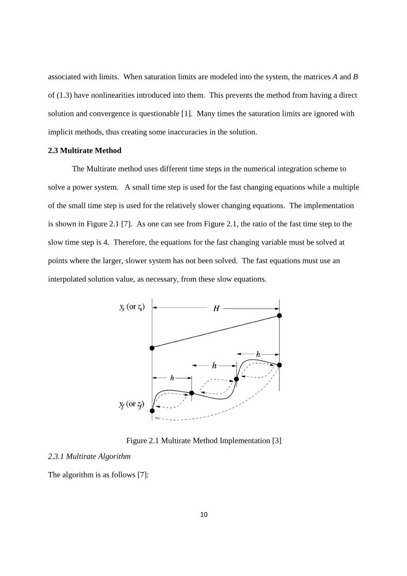
The Multirate method uses different time steps in the numerical integration scheme to

solve a power system. A small time step is used for the fast changing equations while a multiple

of the small time step is used for the relatively slower changing equations. The implementation

is shown in Figure 2.1 [7]. As one can see from Figure 2.1, the ratio of the fast time step to the

slow time step is 4. Therefore, the equations for the fast changing variable must be solved at

points where the larger, slower system has not been solved. The fast equations must use an

interpolated solution value, as necessary, from these slow equations.

Figure 2.1 Multirate Method Implementation [3]

2.3.1 Multirate Algorithm

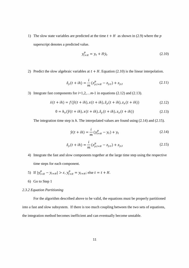
The algorithm is as follows [7]:

11

1) The slow state variables are predicted at the time � � ; as shown in (2.9) where the <

superscript denotes a predicted value.

2) Predict the slow algebraic variables at � � ;. Equation (2.10) is the linear interpolation.

3) Integrate fast components for i=1,2,…m-1 in equations (2.12) and (2.13).

The integration time step is �. The interpolated values are found using (2.14) and (2.15).

4) Integrate the fast and slow components together at the large time step using the respective

time steps for each component.

5) If |�9=>? 6 �9=>| @ A, �9=>? � �9=>; else � � � � ;. 6) Go to Step 1

2.3.2 Equation Partitioning

For the algorithm described above to be valid, the equations must be properly partitioned

into a fast and slow subsystem. If there is too much coupling between the two sets of equations,

the integration method becomes inefficient and can eventually become unstable.

�9=>? � �9 �;��9 (2.10)

CE�� � ��� � �F �CE,9=>? 6 CE,9� � CE,9 (2.11)

�� �� � ��� � ���G�� � ���, ��� � ���, CE�� � ���, C.�� � ���� (2.12)

0 � �.��G�� � ���, ��� � ���, CE�� � ���, C.�� � ���� (2.13)

�G�� � ��� � �F ��9=>? 6 �9� � �9 (2.14)

CE�� � ��� � �F �CE,9=>? 6 CE,9� � CE,9 (2.15)

12

The Multirate method achieves speed-up when the ratio of the number of fast variables to

the number of slow variables is great. Since most power systems have a large number of buses

compared to generators, there will be a greater number of algebraic variables than state variables.

This naturally warrants using the Multirate method for a large system because the ratio of slow to

fast variables is guaranteed to be large [7].

Besides the ratio of slow to fast components, the local truncation error plays a strong role

in determining the partitioning of the state variables. When the local truncation error is large, the

state variable is changing rapidly. Therefore, when state variables have a large local truncation

error (LTE), they can be considered fast variables. The error analysis of the Multirate method is

detailed in [8].

13

CHAPTER 3 METHODOLOGY

3.1 Procedure

To study the Multirate method, power system transient stability simulations are

performed. PowerWorld Simulator is the simulation software package used in the transient

analysis studies. This software package includes a feature to use “subintervals” on any control or

machine model applied to the system. The subintervals allow the operator to use smaller time

steps when the model is solved in the integration method used in the software.

Two main power systems are used in the study. The first system is a small 4-bus system

and the other is a large industry modeled power system. The transient stability tool of the

simulator is mainly used in the simulation and analysis of the two systems. Within each system,

individual control models and generator models with known fast transients are considered. The

behavior of the system’s stability due to the nature of the models is a major focus.

To start, a default simulation with default model parameters is run using a small time

step. This gives a system solution with which to compare subsequent simulation runs. Bus

voltage magnitude and voltage angle data are used as a basis for demonstration of system

stability. A simulation is considered stable when the simulation in question converges to within

5% of the default value for the bus voltage and 10% of the default value for the bus voltage angle

within a reasonable time frame.

Basic control method analysis is used to help determine which control models have a

significant effect on the stability of the system. Three exciter models are studied as they seem to

have a large impact on the overall system stability with regard to the large system. These include

the EXST1_GE, EXAC1, and EXDC2_GE models. Block diagrams of these models are from

PowerWorld Simulator but are publicly available and can be seen in Figures A.1-A.3. Each

14

control model contributes fast decaying transients. These transients arise from feedback loops

determined as fast using basic control theory.

Parameter variation is executed on the models to determine how the system reacts to

perturbations. The changing of parameters allows the user some insight into the control model.

When a parameter is changed, the eigenvalues of the model will change. The insight from basic

control theory analysis of the model block diagrams helps the user regulate which parameters

have the greatest effect on eigenvalues.

After any parameters are changed, a new simulation is run. Bus voltage magnitude and

voltage angle data of the bus with the largest eigenvalue are considered. With the constraints

mentioned before, the simulation is determined as stable or unstable. For unstable simulations,

the next step is to apply subintervals to the model contributing to the large eigenvalue. The

subintervals considered are 2, 4, 8, 16, 32, 64, and 128. These numbers correspond to the ratio

of the system time step to the smaller time step to be used on the individual model. Results of the

simulations on each system are discussed in the following sections.

3.2 Eigenanalysis

Eigenvalue analysis becomes an important tool when studying large power systems. It

allows an operator to understand the various dynamics related to a generator and its associated

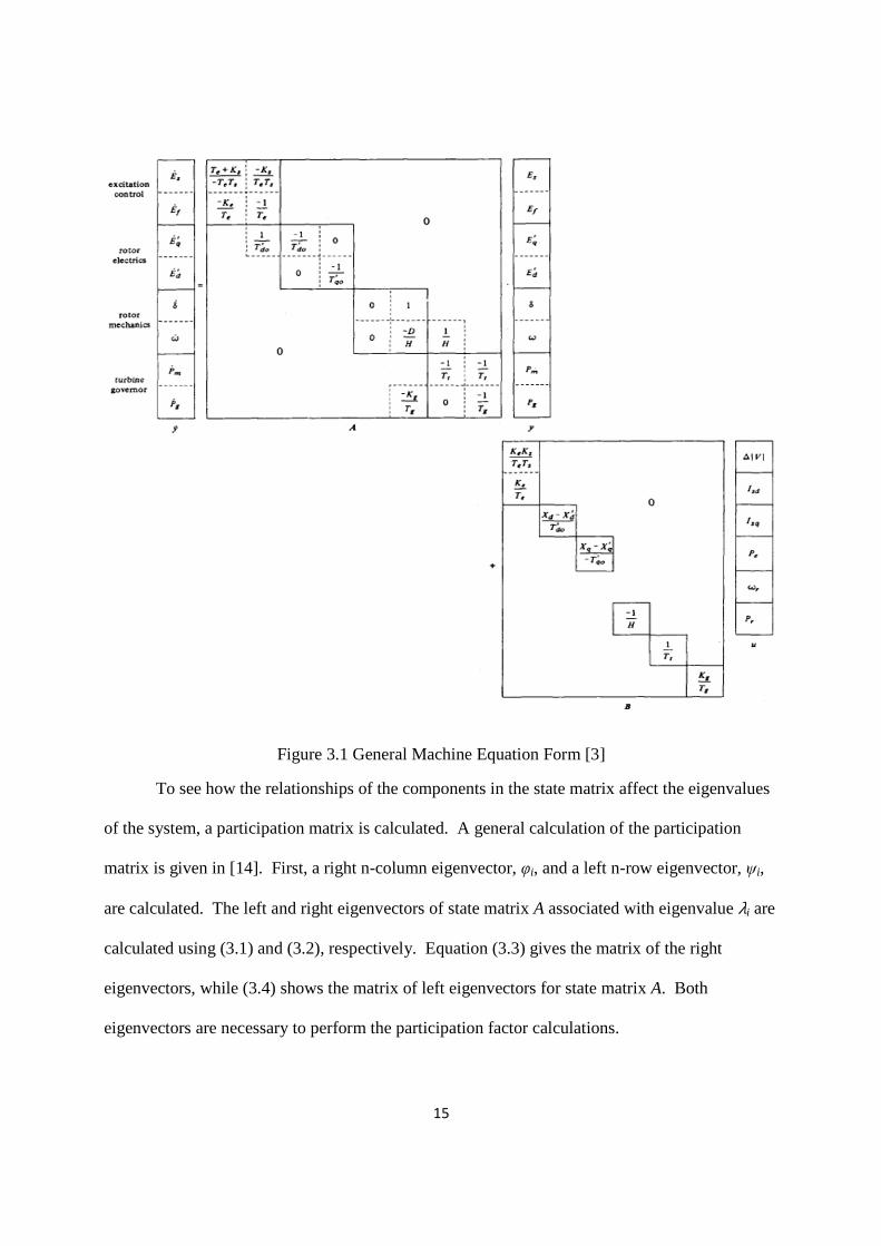
control models. The results of a stability study include the A matrix. Figure 3.1 shows the

general form of equation (1.3) [1]. As seen in Figure 3.1, the A matrix contains the coupling

between the different components of the machine and control models, the state variables.

15

Figure 3.1 General Machine Equation Form [3]

To see how the relationships of the components in the state matrix affect the eigenvalues

of the system, a participation matrix is calculated. A general calculation of the participation

matrix is given in [14]. First, a right n-column eigenvector, φi, and a left n-row eigenvector, ψi,

are calculated. The left and right eigenvectors of state matrix A associated with eigenvalue λi are

calculated using (3.1) and (3.2), respectively. Equation (3.3) gives the matrix of the right

eigenvectors, while (3.4) shows the matrix of left eigenvectors for state matrix A. Both

eigenvectors are necessary to perform the participation factor calculations.

16

I/ � +/I/ (3.1)

J/ � +/J/ (3.2)

K � LI�I�I!…I�N (3.3)

O � LJ�PJ�PJ!P…J�PNP (3.4)

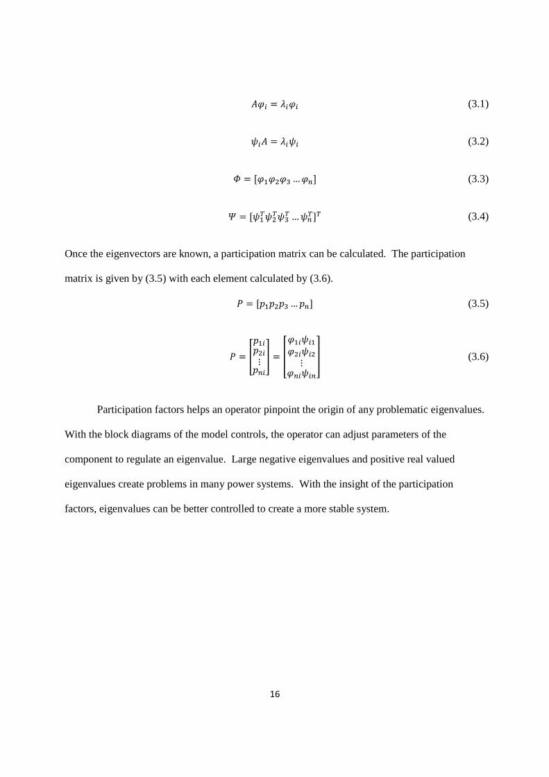
Once the eigenvectors are known, a participation matrix can be calculated. The participation

matrix is given by (3.5) with each element calculated by (3.6).

Q � L<�<�<!…<�N (3.5)

Q � R<�/<�/⋮<�/T � UI�/J/�I�/J/�⋮I�/J/�V (3.6)

Participation factors helps an operator pinpoint the origin of any problematic eigenvalues.

With the block diagrams of the model controls, the operator can adjust parameters of the

component to regulate an eigenvalue. Large negative eigenvalues and positive real valued

eigenvalues create problems in many power systems. With the insight of the participation

factors, eigenvalues can be better controlled to create a more stable system.

17

CHAPTER 4 SYSTEMS OF STUDY

4.1 Small System

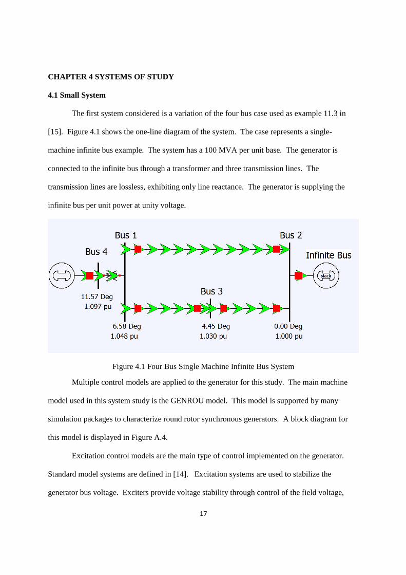
The first system considered is a variation of the four bus case used as example 11.3 in

[15]. Figure 4.1 shows the one-line diagram of the system. The case represents a single-

machine infinite bus example. The system has a 100 MVA per unit base. The generator is

connected to the infinite bus through a transformer and three transmission lines. The

transmission lines are lossless, exhibiting only line reactance. The generator is supplying the

infinite bus per unit power at unity voltage.

Figure 4.1 Four Bus Single Machine Infinite Bus System

Multiple control models are applied to the generator for this study. The main machine

model used in this system study is the GENROU model. This model is supported by many

simulation packages to characterize round rotor synchronous generators. A block diagram for

this model is displayed in Figure A.4.

Excitation control models are the main type of control implemented on the generator.

Standard model systems are defined in [14]. Excitation systems are used to stabilize the

generator bus voltage. Exciters provide voltage stability through control of the field voltage,

18

. With adjustments to the field voltage, the field current changes and the terminal voltage of

the generator will adjust as well [10]. For each simulation, the same contingency event is used.

At t=1 second, a balanced 3-phase fault is applied to bus 3. The fault is cleared by opening the

lines from 3 to 4 and 3 to 1 at time t=1.34 seconds.

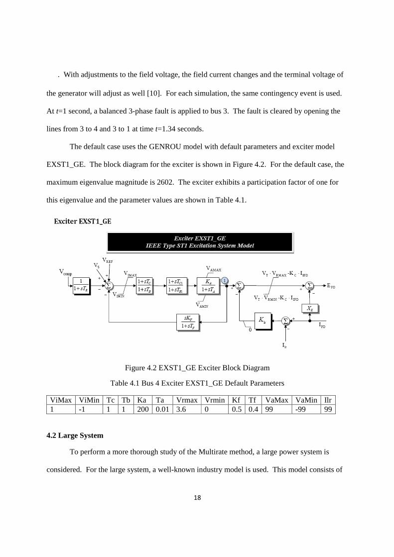
The default case uses the GENROU model with default parameters and exciter model

EXST1_GE. The block diagram for the exciter is shown in Figure 4.2. For the default case, the

maximum eigenvalue magnitude is 2602. The exciter exhibits a participation factor of one for

this eigenvalue and the parameter values are shown in Table 4.1.

Figure 4.2 EXST1_GE Exciter Block Diagram

Table 4.1 Bus 4 Exciter EXST1_GE Default Parameters

ViMax ViMin Tc Tb Ka Ta Vrmax Vrmin Kf Tf VaMax VaMin Ilr 1 -1 1 1 200 0.01 3.6 0 0.5 0.4 99 -99 99

4.2 Large System

To perform a more thorough study of the Multirate method, a large power system is

considered. For the large system, a well-known industry model is used. This model consists of

19

16,386 buses, 3,246 generators, and 8,106 system loads. Two contingency events occur in the

system of study. Two generators are opened at time t=1.0 seconds. The generators remain open

and the system settles to a steady state. Simulations are run for 35 seconds to obtain a reasonable

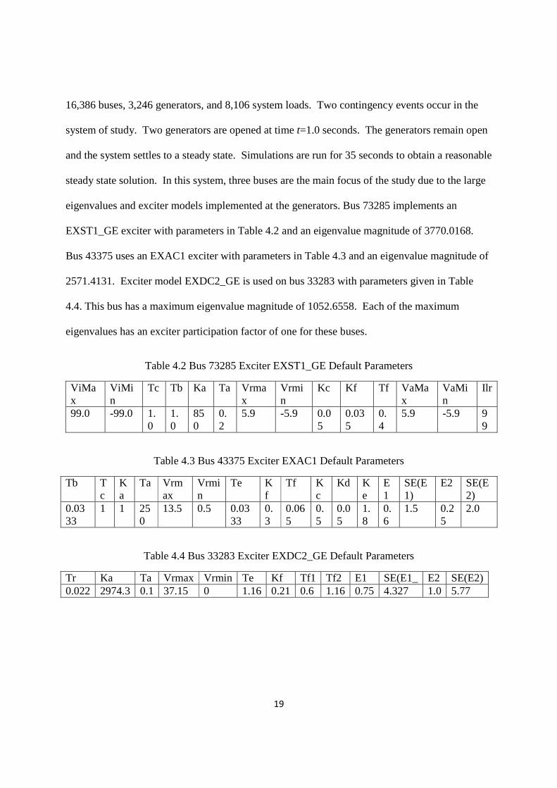
steady state solution. In this system, three buses are the main focus of the study due to the large

eigenvalues and exciter models implemented at the generators. Bus 73285 implements an

EXST1_GE exciter with parameters in Table 4.2 and an eigenvalue magnitude of 3770.0168.

Bus 43375 uses an EXAC1 exciter with parameters in Table 4.3 and an eigenvalue magnitude of

2571.4131. Exciter model EXDC2_GE is used on bus 33283 with parameters given in Table

4.4. This bus has a maximum eigenvalue magnitude of 1052.6558. Each of the maximum

eigenvalues has an exciter participation factor of one for these buses.

Table 4.2 Bus 73285 Exciter EXST1_GE Default Parameters

ViMax

ViMin

Tc Tb Ka Ta Vrmax

Vrmin

Kc Kf Tf VaMax

VaMin

Ilr

99.0 -99.0 1.0

1.0

850

0.2

5.9 -5.9 0.05

0.035

0.4

5.9 -5.9 99

Table 4.3 Bus 43375 Exciter EXAC1 Default Parameters

Tb Tc

Ka

Ta Vrmax

Vrmin

Te Kf

Tf Kc

Kd Ke

E1

SE(E1)

E2 SE(E2)

0.0333

1 1 250

13.5 0.5 0.0333

0.3

0.065

0.5

0.05

1.8

0.6

1.5 0.25

2.0

Table 4.4 Bus 33283 Exciter EXDC2_GE Default Parameters

Tr Ka Ta Vrmax Vrmin Te Kf Tf1 Tf2 E1 SE(E1_ E2 SE(E2) 0.022 2974.3 0.1 37.15 0 1.16 0.21 0.6 1.16 0.75 4.327 1.0 5.77

20

CHAPTER 5 DISCUSSION OF RESULTS

5.1 Eigenvalue Limits

Insight into the subinterval effectiveness of maintaining system stability was gained

during the simulations on the small system. During these simulations, parameter variation of all

generator and control models provided different insights into the system. In each case, exciter

models were used with the generator. The exciter models EXST1_GE, EXAC1, and

EXDC2_GE proved to be the most problematic in the system. From the eigenvalue and

participation matrix analysis, the exciter was found to cause stability problems in each simulation

studied. The participation matrix also gives the location of the large eigenvalue on the exciter

model block diagram.

Once the origin of the large eigenvalue of the system is known, the parameters

contributing to the large eigenvalue are varied. First, the EXST1_GE exciter was studied. The

first feedback loop shown in Figure 4.1 caused the greatest response to the large eigenvalues of

the system. Parameters of this feedback loop were varied to change the magnitude of the largest

eigenvalue. A subinterval was placed on the exciter system and the feedback loop parameters

were changed until the system lost stability. This was repeated for each subinterval value and for

the EXAC1 and EXDC2_GE exciter models as well.

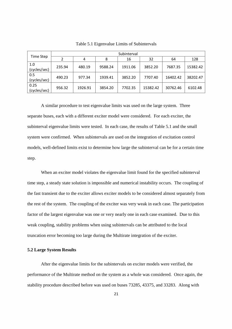
In each exciter case, the results were very similar. The exciter contributed a participation

factor of 1 to the largest eigenvalue magnitude in each case. Table 5.1 shows the upper

eigenvalue limits for stability of the system when using the specified subinterval on the

excitation model and integration time step. The eigenvalue stability limits for each of the exciter

models were very close to one another and the values in the table are the limit averages.

21

Table 5.1 Eigenvalue Limits of Subintervals

Time Step Subinterval

2 4 8 16 32 64 128

1.0

(cycles/sec) 235.94 480.19 9588.24 1911.06 3852.20 7687.35 15382.42

0.5

(cycles/sec) 490.23 977.34 1939.41 3852.20 7707.40 16402.42 38202.47

0.25

(cycles/sec) 956.32 1926.91 3854.20 7702.35 15382.42 30762.46 6102.48

A similar procedure to test eigenvalue limits was used on the large system. Three

separate buses, each with a different exciter model were considered. For each exciter, the

subinterval eigenvalue limits were tested. In each case, the results of Table 5.1 and the small

system were confirmed. When subintervals are used on the integration of excitation control

models, well-defined limits exist to determine how large the subinterval can be for a certain time

step.

When an exciter model violates the eigenvalue limit found for the specified subinterval

time step, a steady state solution is impossible and numerical instability occurs. The coupling of

the fast transient due to the exciter allows exciter models to be considered almost separately from

the rest of the system. The coupling of the exciter was very weak in each case. The participation

factor of the largest eigenvalue was one or very nearly one in each case examined. Due to this

weak coupling, stability problems when using subintervals can be attributed to the local

truncation error becoming too large during the Multirate integration of the exciter.

5.2 Large System Results

After the eigenvalue limits for the subintervals on exciter models were verified, the

performance of the Multirate method on the system as a whole was considered. Once again, the

stability procedure described before was used on buses 73285, 43375, and 33283. Along with

22

the convergence of the bus voltage magnitude and voltage angle, the integration solution details

of the system are used to judge the performance of a solution run. The solution results include

the overall simulation time, maximum angle difference, time of the maximum angle difference,

total number of Newton solutions, number of Jacobian factorizations, and the number of forward

and backward substitutions. For each simulation run, the same computer was used so as to keep

consistency with the simulation time.

A default simulation run with a time step of 0.1 cycles was run to give a steady state

value to prove convergence of the bus voltage magnitude and voltage angle. The eigenvalue

limits in Table 5.1 help when determining an appropriate subinterval to place on the exciter

model. The same three system time steps were examined. For each time step, a myriad of

different combinations were considered when placing subintervals on system components

including machine models and stabilizers. No definite conclusion or intuition was gained

through these simulations, so the focus of the study returned to studying the effect of the

Multirate method on excitation controls.

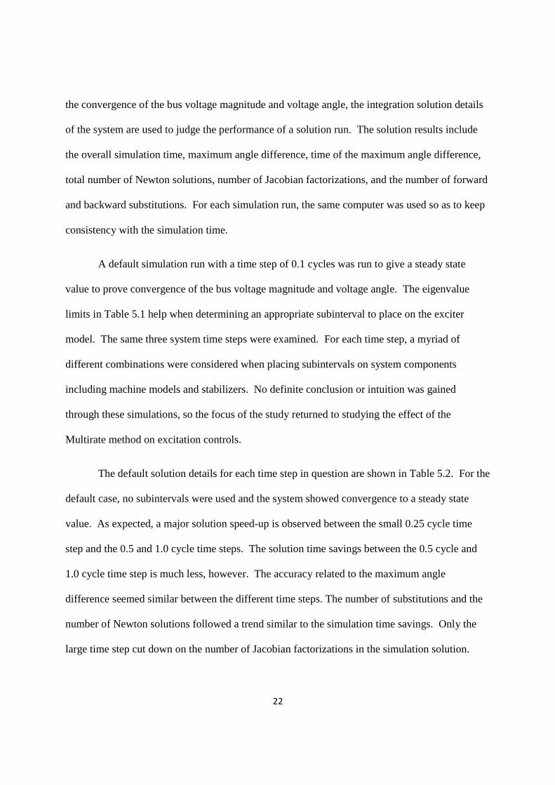
The default solution details for each time step in question are shown in Table 5.2. For the

default case, no subintervals were used and the system showed convergence to a steady state

value. As expected, a major solution speed-up is observed between the small 0.25 cycle time

step and the 0.5 and 1.0 cycle time steps. The solution time savings between the 0.5 cycle and

1.0 cycle time step is much less, however. The accuracy related to the maximum angle

difference seemed similar between the different time steps. The number of substitutions and the

number of Newton solutions followed a trend similar to the simulation time savings. Only the

large time step cut down on the number of Jacobian factorizations in the simulation solution.

23

Table 5.2 Default Simulation Solution Details

0.25 cycles 0.5 cycles 1.0 cycles Sim. Time (secs) 1015.753 535.115 450.203 Max. Angle Diff. (Deg)

397.118 397.010 397.300

Time of Max Angle Difference (secs)

4.358 4.358 4.367

Total Newton Solutions

12622 6325 4174

Jacobian Factorizations

73 73 71

Forward/Backward Subs

12345 6205 4183

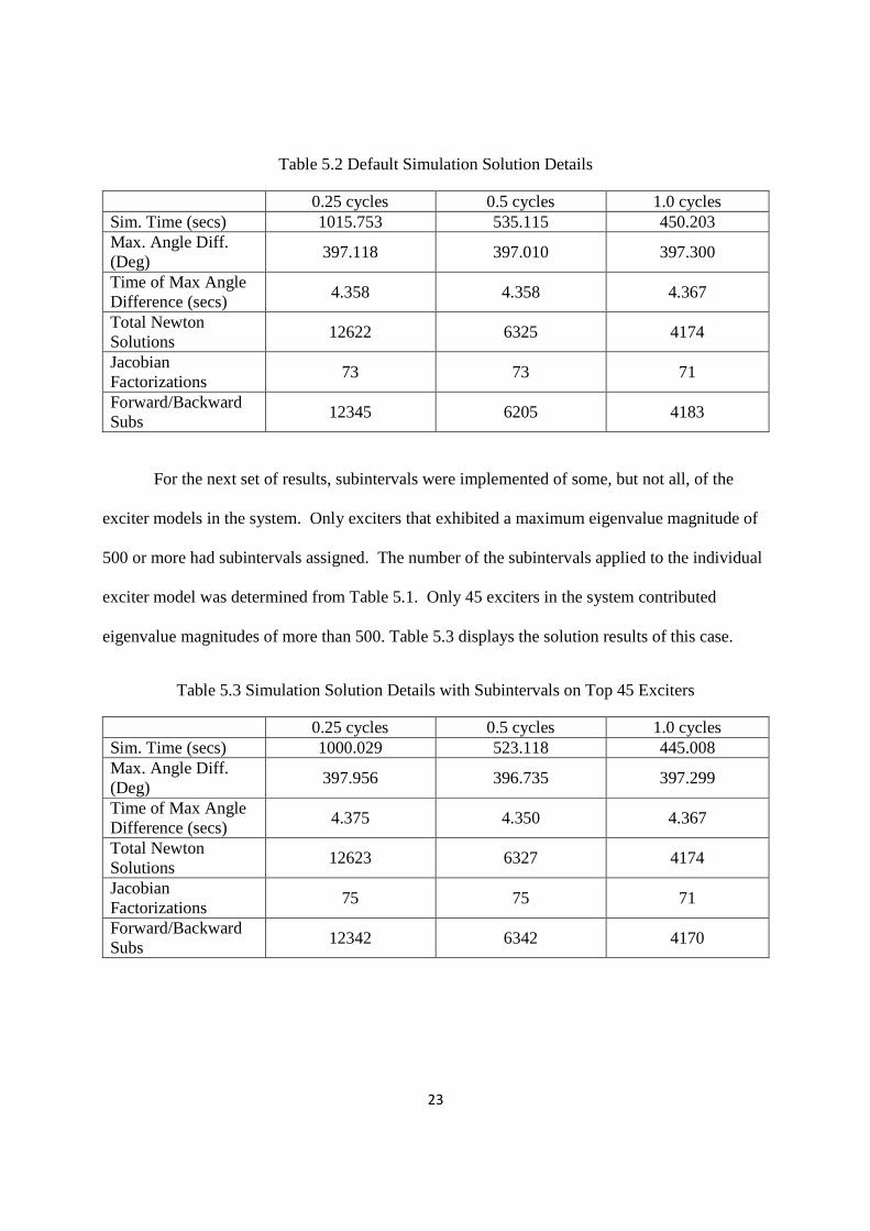
For the next set of results, subintervals were implemented of some, but not all, of the

exciter models in the system. Only exciters that exhibited a maximum eigenvalue magnitude of

500 or more had subintervals assigned. The number of the subintervals applied to the individual

exciter model was determined from Table 5.1. Only 45 exciters in the system contributed

eigenvalue magnitudes of more than 500. Table 5.3 displays the solution results of this case.

Table 5.3 Simulation Solution Details with Subintervals on Top 45 Exciters

0.25 cycles 0.5 cycles 1.0 cycles Sim. Time (secs) 1000.029 523.118 445.008 Max. Angle Diff. (Deg)

397.956 396.735 397.299

Time of Max Angle Difference (secs)

4.375 4.350 4.367

Total Newton Solutions

12623 6327 4174

Jacobian Factorizations

75 75 71

Forward/Backward Subs

12342 6342 4170

24

For each time step, little solution time savings was realized: only 15 seconds for the best

case. Also, additional calculations are necessary for the half-cycle and quarter-cycle time step

solutions.

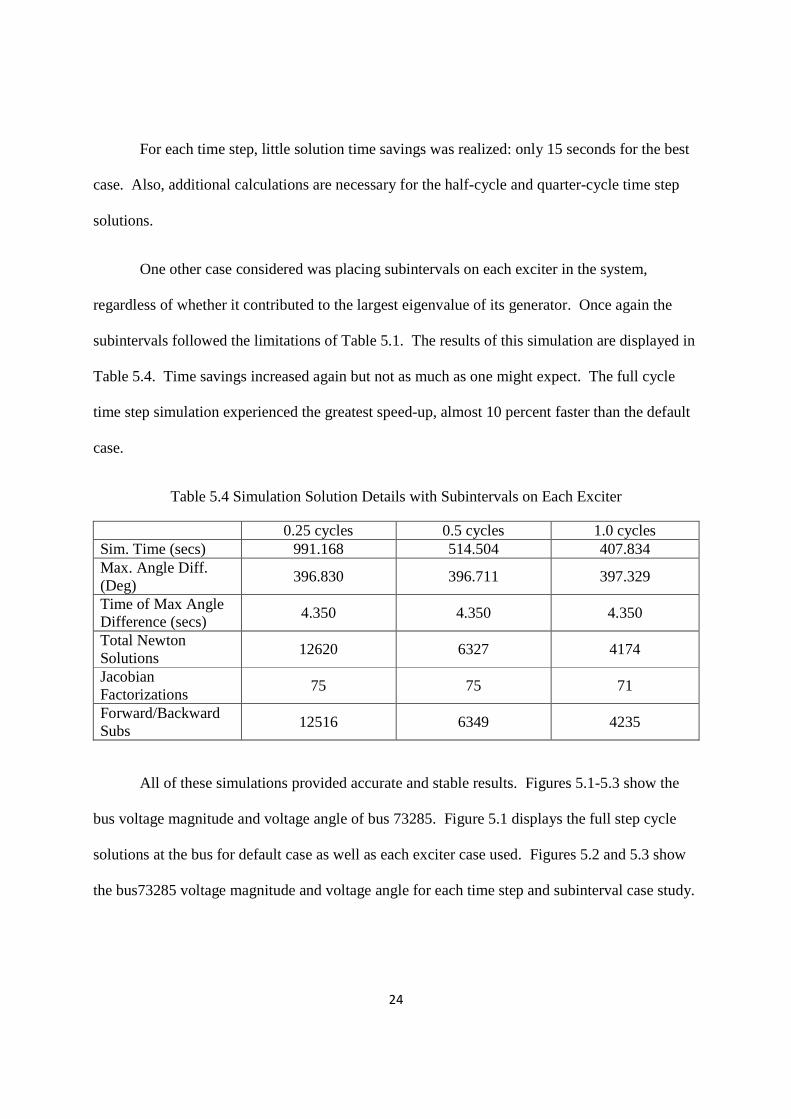
One other case considered was placing subintervals on each exciter in the system,

regardless of whether it contributed to the largest eigenvalue of its generator. Once again the

subintervals followed the limitations of Table 5.1. The results of this simulation are displayed in

Table 5.4. Time savings increased again but not as much as one might expect. The full cycle

time step simulation experienced the greatest speed-up, almost 10 percent faster than the default

case.

Table 5.4 Simulation Solution Details with Subintervals on Each Exciter

0.25 cycles 0.5 cycles 1.0 cycles Sim. Time (secs) 991.168 514.504 407.834 Max. Angle Diff. (Deg)

396.830 396.711 397.329

Time of Max Angle Difference (secs)

4.350 4.350 4.350

Total Newton Solutions

12620 6327 4174

Jacobian Factorizations

75 75 71

Forward/Backward Subs

12516 6349 4235

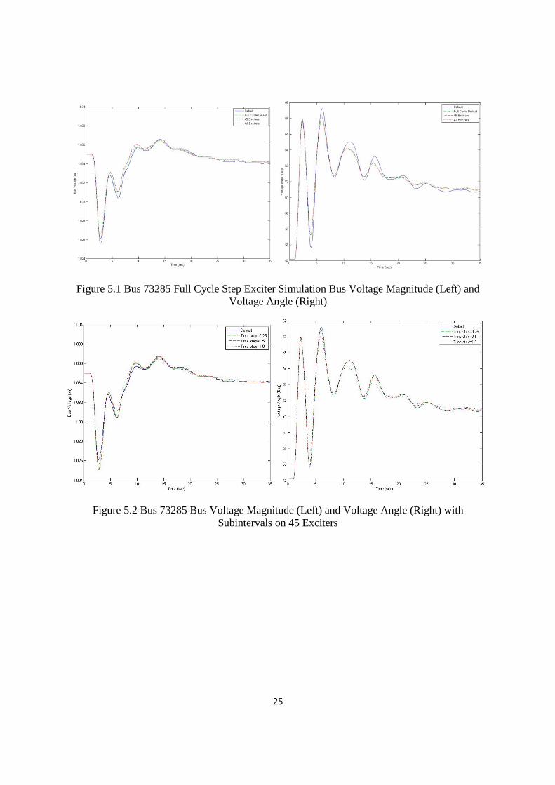
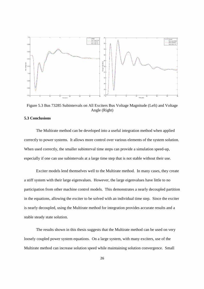
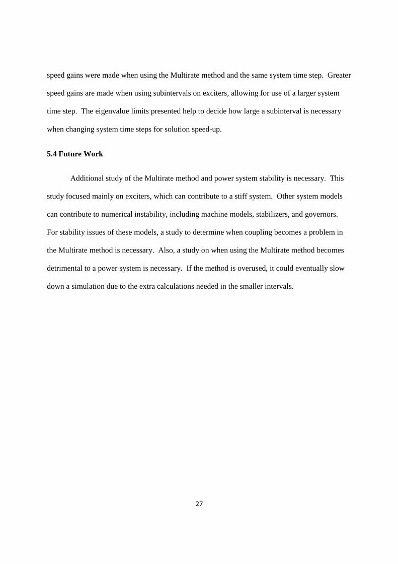
All of these simulations provided accurate and stable results. Figures 5.1-5.3 show the

bus voltage magnitude and voltage angle of bus 73285. Figure 5.1 displays the full step cycle

solutions at the bus for default case as well as each exciter case used. Figures 5.2 and 5.3 show

the bus73285 voltage magnitude and voltage angle for each time step and subinterval case study.

25

Figure 5.1 Bus 73285 Full Cycle Step Exciter Simulation Bus Voltage Magnitude (Left) and Voltage Angle (Right)

Figure 5.2 Bus 73285 Bus Voltage Magnitude (Left) and Voltage Angle (Right) with Subintervals on 45 Exciters

26

Figure 5.3 Bus 73285 Subintervals on All Exciters Bus Voltage Magnitude (Left) and Voltage Angle (Right)

5.3 Conclusions

The Multirate method can be developed into a useful integration method when applied

correctly to power systems. It allows more control over various elements of the system solution.

When used correctly, the smaller subinterval time steps can provide a simulation speed-up,

especially if one can use subintervals at a large time step that is not stable without their use.

Exciter models lend themselves well to the Multirate method. In many cases, they create

a stiff system with their large eigenvalues. However, the large eigenvalues have little to no

participation from other machine control models. This demonstrates a nearly decoupled partition

in the equations, allowing the exciter to be solved with an individual time step. Since the exciter

is nearly decoupled, using the Multirate method for integration provides accurate results and a

stable steady state solution.

The results shown in this thesis suggests that the Multirate method can be used on very

loosely coupled power system equations. On a large system, with many exciters, use of the

Multirate method can increase solution speed while maintaining solution convergence. Small

27

speed gains were made when using the Multirate method and the same system time step. Greater

speed gains are made when using subintervals on exciters, allowing for use of a larger system

time step. The eigenvalue limits presented help to decide how large a subinterval is necessary

when changing system time steps for solution speed-up.

5.4 Future Work

Additional study of the Multirate method and power system stability is necessary. This

study focused mainly on exciters, which can contribute to a stiff system. Other system models

can contribute to numerical instability, including machine models, stabilizers, and governors.

For stability issues of these models, a study to determine when coupling becomes a problem in

the Multirate method is necessary. Also, a study on when using the Multirate method becomes

detrimental to a power system is necessary. If the method is overused, it could eventually slow

down a simulation due to the extra calculations needed in the smaller intervals.

28

REFERENCES

[1] B. Stott, “Power system dynamic response calculations,” Proceedings of the IEEE, vol. 67, no. 2, pp. 219-241, Feb. 1979.

[2] D. Koester, S. Ranka, and G. Fox, “Power systems transient stability-a grand computing challenge,” Northeast Parallel Architectures Center, Syracuse, NY, Tech. Rep. SCCS 549, Aug. 1992.

[3] A. Kurita, H. Okubo, K. Oki, S. Agematsu, D. B. Klapper, N. W. Miller, W. W. Price Jr., J. J. Sanchez-Gasca, K. A. Wirgau, and T. D. Younkins, “Multiple time-scale power system dynamic simulation,” IEEE Transactions on Power Systems, vol. 8, no. 1, pp. 216-223, Feb 1993.

[4] C. Gear, “Multirate methods for ordinary differential equations,” University of Illinois at Urbana-Champaign, Tech. Rep. UIUCDCS- 74-880, 1974.

[5] M. L. Crow and J. G. Chen, “The multirate method for simulation of power system dynamics,” IEEE Transactions on Power Systems, vol. 9, no. 3, pp. 1684-1690, Aug 1994.

[6] M. L. Crow and J. G. Chen, “The multirate simulation of FACTS devices in power system dynamics,” IEEE Transactions on Power Systems, vol. 11, no. 1, pp. 376-382, Feb. 1996.

[7] M. L. Crow and J. G. Chen, “A variable partitioning strategy for the multirate method in power systems,” IEEE Transactions on Power Systems, vol. 23, no. 2, pp. 259-266, May 2008.

[8] J. G. Chen, M. L. Crow, B. H. Chowdhury, and L. Acar, “An error analysis of the multirate method for power system transient stability simulation,” Power Systems Conference and Exposition, vol. 2, pp. 982-986, 2004.

[9] P. Kundur, Power System Stability and Control. New York, NY: McGraw-Hill, 1994.

[10] P. W. Sauer and M. A. Pai, Power System Dynamics and Stability. Upper Saddle River, NJ: Prentice Hall, 1997.

[11] G. Gross, “Analysis techniques for large-scale electrical systems,” class notes for ECE 530, Department of Electrical and Computer Engineering, University of Illinois at Urbana-Champaign, Oct. 15, 2009.

[12] P. L. Dandeno and P. Kundur, “A non-iterative transient stability program including the effects of variable load-voltage characteristics,” IEEE Transactions on Power Apparatus and Systems, vol. PAS-92, no. 5, pp. 1478-1484, Sept. 1973.

[13] H. W. Dommel and N. Sato, “Fast transient stability solutions,” IEEE Transactions on Power Apparatus and Systems, vol. PAS-91, no. 4, pp. 1643-1650, July 1972.

29

[14] F. A. Moreira and J. R. Martí, “Latency suitability for the time-domain simulation of electromagnetic transients through network eigenanalysis,” in Proc. Int. Conf. on Power Systems Transients (IPST), New Orleans, LA, 2003, Session 3a, Paper 4. [Online]. Available: http://www.ipst.org/IPST03Papers.htm.

[15] J. D. Glover, M. S. Sarma, and T. J. Overbye, Power System Analysis and Design, 5th ed.

Toronto, Canada: Thomson Learning, 2011.

[16] IEEE Working Group on Computer Modelling of Excitation Systems, “Excitation system models for power system stability studies: IEEE committee report,” IEEE Transactions on Power Apparatus Systems, vol. PAS-100 no. 2, pp. 494-507, Feb. 1981.

30

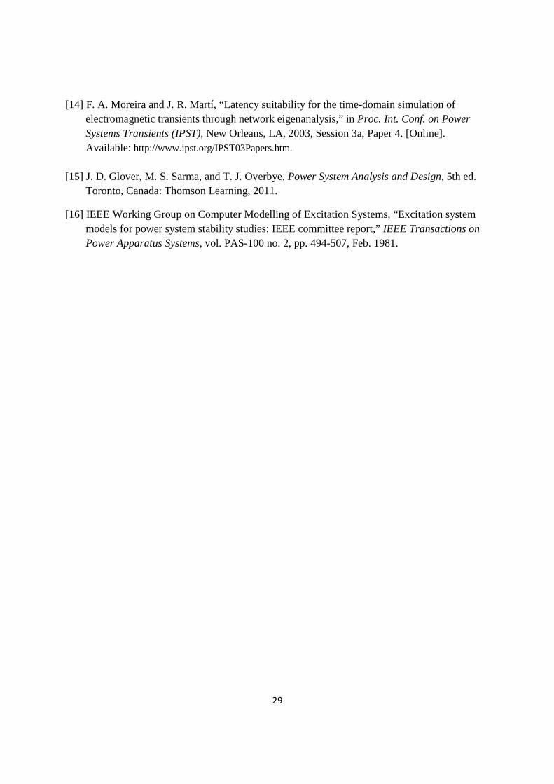
APPENDIX A

MODEL BLOCK DIAGRAMS

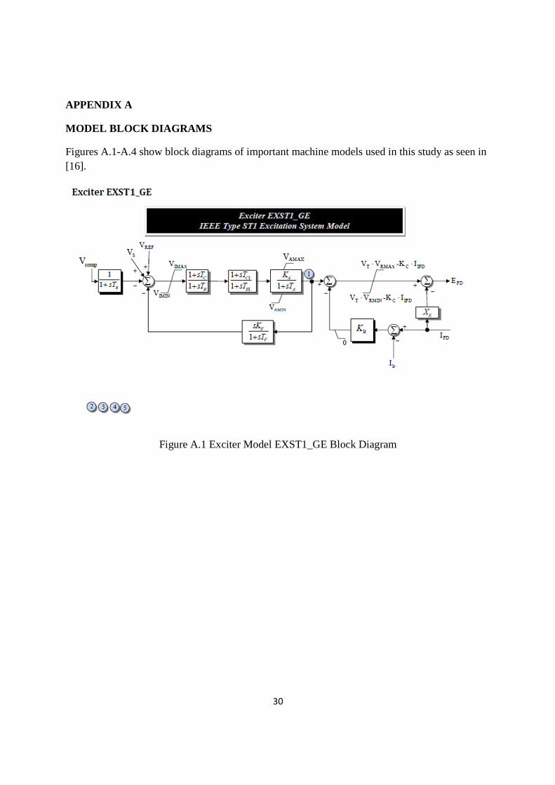
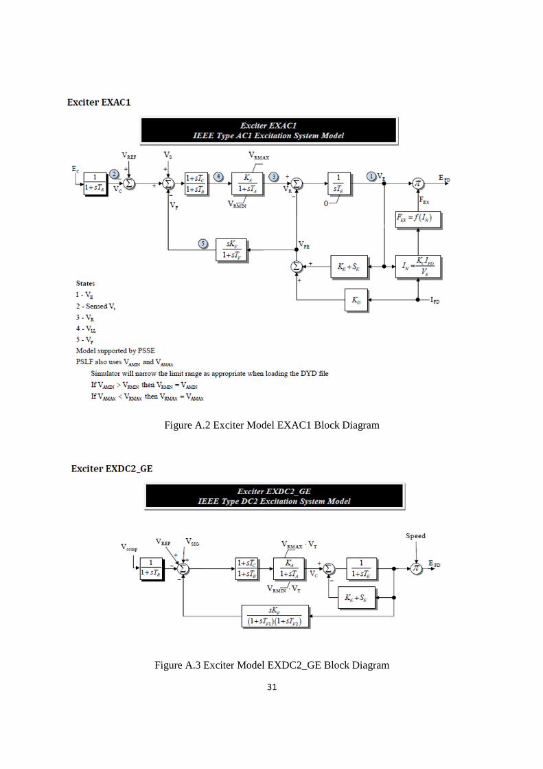
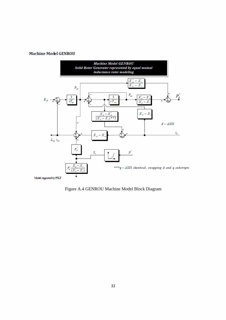
Figures A.1-A.4 show block diagrams of important machine models used in this study as seen in [16].

Figure A.1 Exciter Model EXST1_GE Block Diagram

31

Figure A.2 Exciter Model EXAC1 Block Diagram

Figure A.3 Exciter Model EXDC2_GE Block Diagram

32

Figure A.4 GENROU Machine Model Block Diagram