power system transient stability simulation · ! 1! power system transient stability simulation...
TRANSCRIPT
1
Power System Transient
Stability Simulation
Ashley Cliff
Mentors: Srdjan Simunovic, Aleksandar Dimitrovski, Kwai Wong
2
Overview Electricity is an intrinsic part of modern culture, and having reliable access is a
necessity. Power supply systems, i.e. power grids, have the responsibility to produce and
distribute steady power to all consumers. Due to the nature of power, and of alternating
currents, slight disturbances can cause large amounts of fluctuation and damage quickly.
These can cause power outages that can range in severity from a single downed line to an
entire country or more without power.
The purpose of this project is to create accurate simulations of power outages that
can be used to avoid actual power failures. For the simulations to be useful, they must be
able to run faster than real time, to determine what will happen when there’s an outage
before the outcome occurs. To accomplish this, the Parareal in Time Algorithm is being
implemented to increase speed up and aid in a logical way to parallelize the code.
Steady State System To simulate power outages, one must first be able to simulate and model a steady
state power system that has no issues. A simulation is accurate when the amount of power
generated is very closely matched to the amount of power used, and all voltages and
voltage angles are known. This starts with the physics of electricity, magnetism, and
circuits, and the design of power grids. An accurate representation of a power grid
includes all the lines, buses, transformers, generators, loads, and many other pieces. Each
line has an impedance (z) associated with it, where impedance is the total opposition to
the alternating current (Dictionary.com).
Admittances (y) are more commonly used in calculations, and are the inverses of
each impedance value. The admittances for each line are put into an admittance matrix
(Y) with the diagonal entries being all values flowing into a bus, and the rest being the
value between two buses, with unconnected buses having a value of zero.
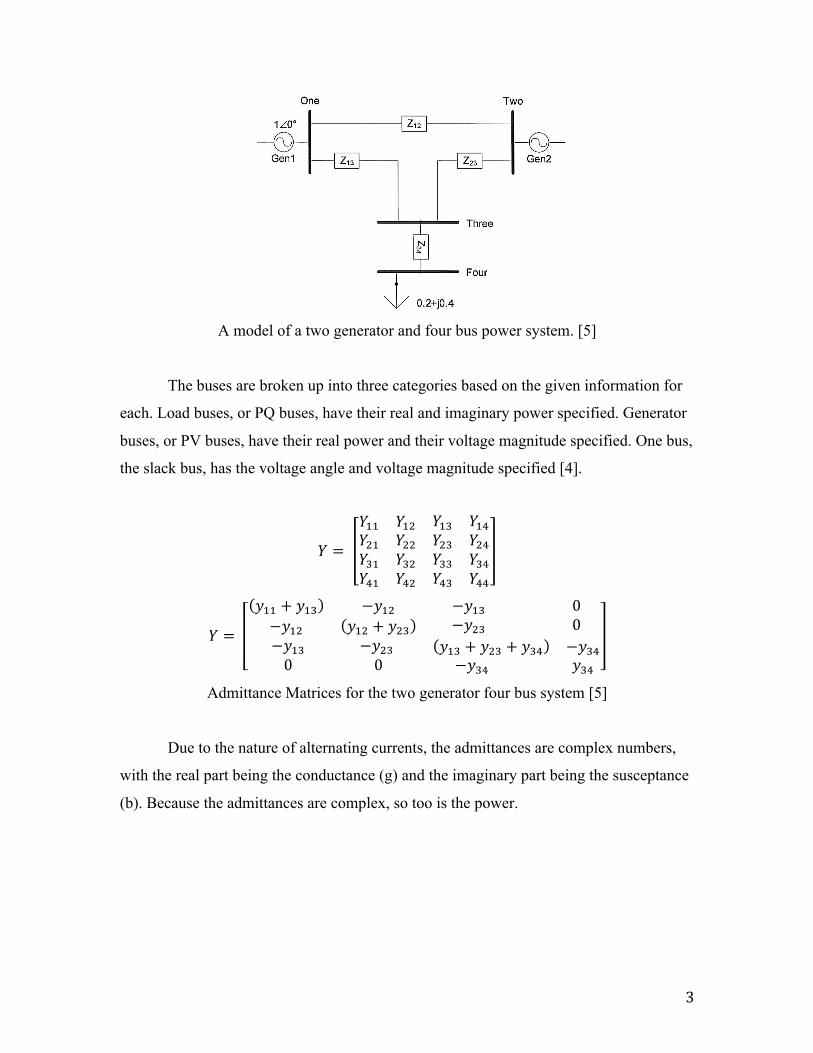
3
A model of a two generator and four bus power system. [5]
The buses are broken up into three categories based on the given information for
each. Load buses, or PQ buses, have their real and imaginary power specified. Generator
buses, or PV buses, have their real power and their voltage magnitude specified. One bus,
the slack bus, has the voltage angle and voltage magnitude specified [4].
𝑌 =
𝑌!! 𝑌!"𝑌!" 𝑌!!
𝑌!" 𝑌!"𝑌!" 𝑌!"
𝑌!" 𝑌!!𝑌!" 𝑌!"
𝑌!! 𝑌!"𝑌!" 𝑌!!
𝑌 =
𝑦!! + 𝑦!" −𝑦!"−𝑦!" 𝑦!" + 𝑦!"
−𝑦!" 0−𝑦!" 0
−𝑦!" −𝑦!"0 0
𝑦!" + 𝑦!" + 𝑦!" −𝑦!"−𝑦!" 𝑦!"
Admittance Matrices for the two generator four bus system [5]
Due to the nature of alternating currents, the admittances are complex numbers,
with the real part being the conductance (g) and the imaginary part being the susceptance
(b). Because the admittances are complex, so too is the power.
4
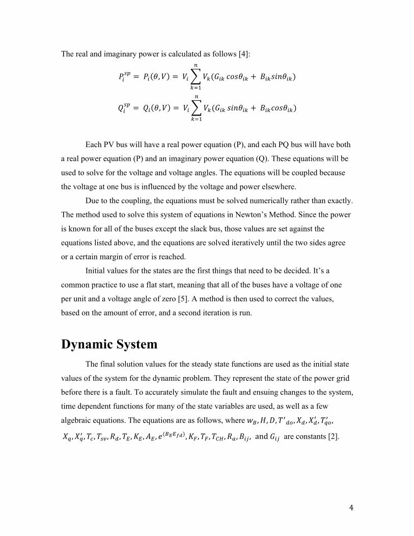
The real and imaginary power is calculated as follows [4]:
𝑃!!" = 𝑃! 𝜃,𝑉 = 𝑉! 𝑉!(𝐺!"
!
!!!
𝑐𝑜𝑠𝜃!" + 𝐵!"𝑠𝑖𝑛𝜃!")
𝑄!!" = 𝑄! 𝜃,𝑉 = 𝑉! 𝑉!(𝐺!"
!
!!!
𝑠𝑖𝑛𝜃!" + 𝐵!"𝑐𝑜𝑠𝜃!")
Each PV bus will have a real power equation (P), and each PQ bus will have both
a real power equation (P) and an imaginary power equation (Q). These equations will be
used to solve for the voltage and voltage angles. The equations will be coupled because
the voltage at one bus is influenced by the voltage and power elsewhere.
Due to the coupling, the equations must be solved numerically rather than exactly.
The method used to solve this system of equations in Newton’s Method. Since the power
is known for all of the buses except the slack bus, those values are set against the
equations listed above, and the equations are solved iteratively until the two sides agree
or a certain margin of error is reached.
Initial values for the states are the first things that need to be decided. It’s a
common practice to use a flat start, meaning that all of the buses have a voltage of one
per unit and a voltage angle of zero [5]. A method is then used to correct the values,
based on the amount of error, and a second iteration is run.
Dynamic System The final solution values for the steady state functions are used as the initial state
values of the system for the dynamic problem. They represent the state of the power grid
before there is a fault. To accurately simulate the fault and ensuing changes to the system,
time dependent functions for many of the state variables are used, as well as a few
algebraic equations. The equations are as follows, where 𝑤! ,𝐻,𝐷,𝑇!!" ,𝑋! ,𝑋!! ,𝑇!"! ,
𝑋! ,𝑋!! ,𝑇! ,𝑇!" ,𝑅! ,𝑇! ,𝐾! ,𝐴! , 𝑒(!!!!"),𝐾! ,𝑇! ,𝑇!" ,𝑅! ,𝐵!" , and 𝐺!" are constants [2].
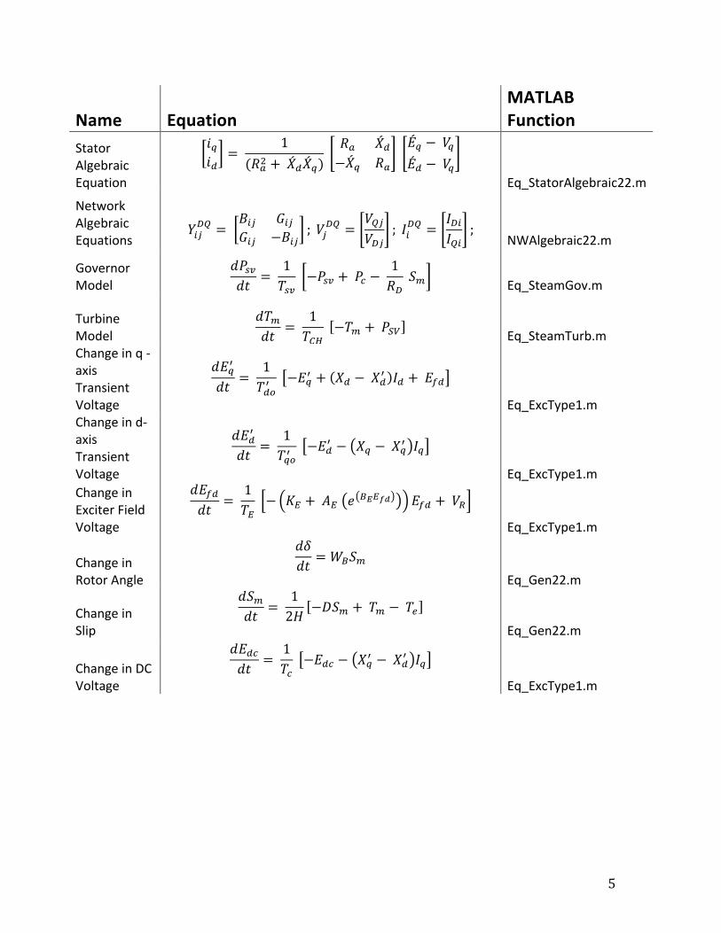
5
Name Equation MATLAB Function
Stator Algebraic Equation
𝑖!𝑖!
= 1
(𝑅!! + 𝑋!𝑋!) 𝑅! 𝑋!−𝑋! 𝑅!
𝐸! − 𝑉!𝐸! − 𝑉!
Eq_StatorAlgebraic22.m
Network Algebraic Equations
𝑌!"!" =
𝐵!" 𝐺!"𝐺!" −𝐵!"
; 𝑉!!" =
𝑉!"𝑉!"
; 𝐼!!" =
𝐼!"𝐼!"
; NWAlgebraic22.m
Governor Model
𝑑𝑃!"𝑑𝑡 =
1𝑇!"
−𝑃!" + 𝑃! − 1𝑅! 𝑆! Eq_SteamGov.m
Turbine Model
𝑑𝑇!𝑑𝑡 =
1𝑇!"
−𝑇! + 𝑃!" Eq_SteamTurb.m Change in q -‐ axis Transient Voltage
𝑑𝐸!!
𝑑𝑡 = 1𝑇!"!
−𝐸!! + 𝑋! − 𝑋!! 𝐼! + 𝐸!"
Eq_ExcType1.m Change in d-‐ axis Transient Voltage
𝑑𝐸!!
𝑑𝑡 = 1𝑇!"!
−𝐸!! − 𝑋! − 𝑋!! 𝐼!
Eq_ExcType1.m Change in Exciter Field Voltage
𝑑𝐸!"𝑑𝑡 =
1𝑇! − 𝐾! + 𝐴! 𝑒 !!!!" 𝐸!" + 𝑉!
Eq_ExcType1.m
Change in Rotor Angle
𝑑𝛿𝑑𝑡 =𝑊!𝑆!
Eq_Gen22.m
Change in Slip
𝑑𝑆!𝑑𝑡 =
12𝐻 −𝐷𝑆! + 𝑇! − 𝑇!
Eq_Gen22.m
Change in DC Voltage
𝑑𝐸!"𝑑𝑡 =
1𝑇! −𝐸!" − 𝑋!! − 𝑋!! 𝐼!
Eq_ExcType1.m
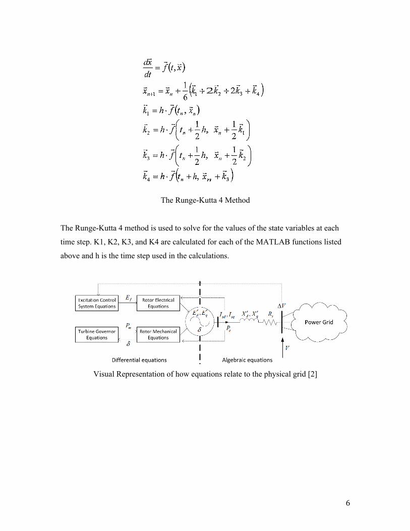
6
The Runge-Kutta 4 Method
The Runge-Kutta 4 method is used to solve for the values of the state variables at each
time step. K1, K2, K3, and K4 are calculated for each of the MATLAB functions listed
above and h is the time step used in the calculations.
Visual Representation of how equations relate to the physical grid [2]
7
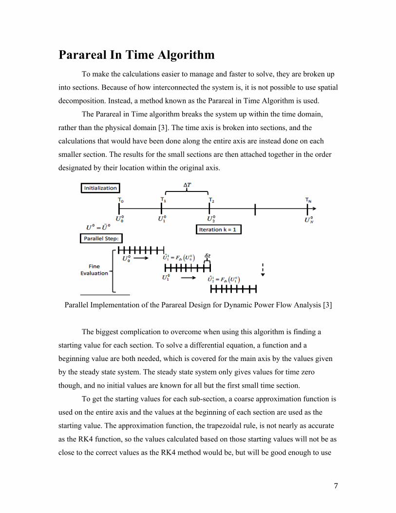
Parareal In Time Algorithm To make the calculations easier to manage and faster to solve, they are broken up
into sections. Because of how interconnected the system is, it is not possible to use spatial
decomposition. Instead, a method known as the Parareal in Time Algorithm is used.
The Parareal in Time algorithm breaks the system up within the time domain,
rather than the physical domain [3]. The time axis is broken into sections, and the
calculations that would have been done along the entire axis are instead done on each
smaller section. The results for the small sections are then attached together in the order
designated by their location within the original axis.
Parallel Implementation of the Parareal Design for Dynamic Power Flow Analysis [3]
The biggest complication to overcome when using this algorithm is finding a
starting value for each section. To solve a differential equation, a function and a
beginning value are both needed, which is covered for the main axis by the values given
by the steady state system. The steady state system only gives values for time zero
though, and no initial values are known for all but the first small time section.
To get the starting values for each sub-section, a coarse approximation function is
used on the entire axis and the values at the beginning of each section are used as the
starting value. The approximation function, the trapezoidal rule, is not nearly as accurate
as the RK4 function, so the values calculated based on those starting values will not be as
close to the correct values as the RK4 method would be, but will be good enough to use
8
as a starting point. Once a fine solve iteration has run, the coarse value is corrected, the
coarse method is reran with a more accurate value and the system runs again. This
iterative method is used until the value is within a specified margin of error, or the
maximum number of iterations is reached.
To make this process run faster than simply solving each time step one after the
other, the calculations for each of the sub-intervals are done in parallel. When the number
of sub-intervals is large, doing the calculations in parallel can provide a significant speed
up. The speed up is offset by the time it takes for the coarse solver and coarse corrector to
run, which a simple serial calculation would not have.
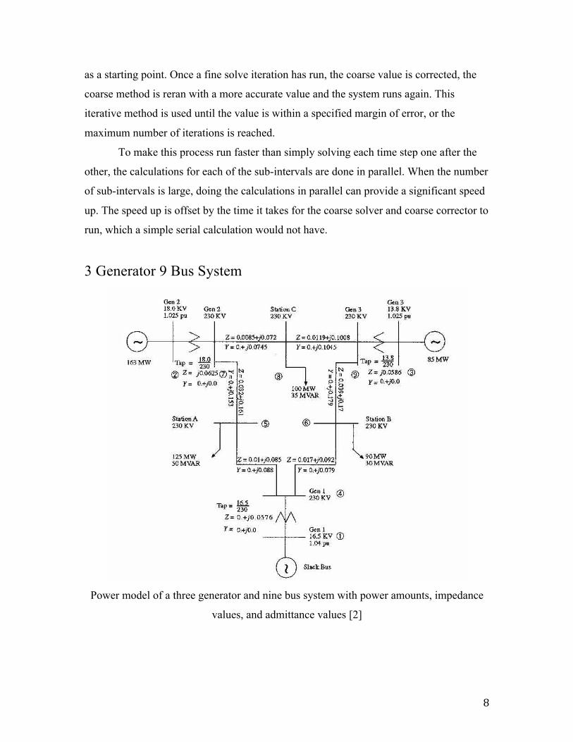
3 Generator 9 Bus System
Power model of a three generator and nine bus system with power amounts, impedance
values, and admittance values [2]
9
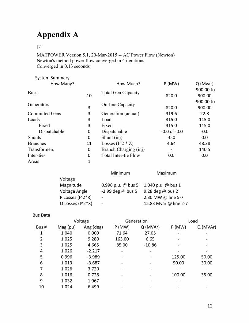
The starting values for the 3 generator 9 bus system are as shown in the above
diagram. The steady state system is solved using MatPower (matpower5.1) [7], a module
added into the MATLAB code framework. Results in Appendix A. All results have been
found using this system.
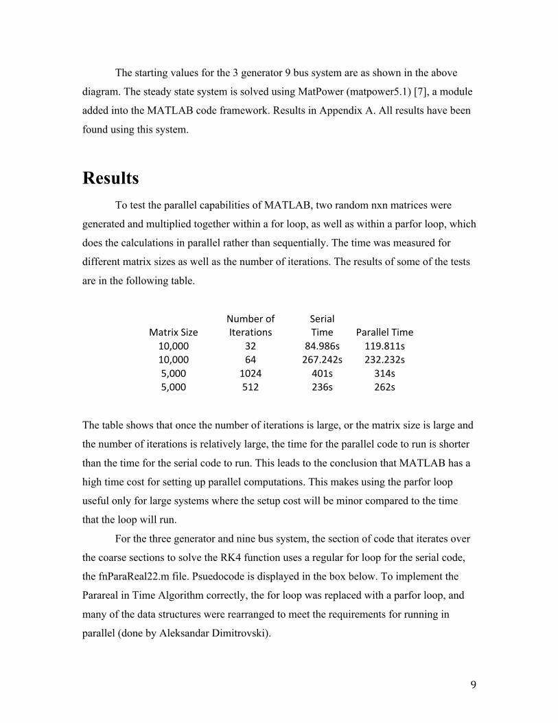
Results To test the parallel capabilities of MATLAB, two random nxn matrices were
generated and multiplied together within a for loop, as well as within a parfor loop, which
does the calculations in parallel rather than sequentially. The time was measured for
different matrix sizes as well as the number of iterations. The results of some of the tests
are in the following table.
Matrix Size Number of Iterations
Serial Time Parallel Time
10,000 32 84.986s 119.811s 10,000 64 267.242s 232.232s 5,000 1024 401s 314s 5,000 512 236s 262s
The table shows that once the number of iterations is large, or the matrix size is large and
the number of iterations is relatively large, the time for the parallel code to run is shorter
than the time for the serial code to run. This leads to the conclusion that MATLAB has a
high time cost for setting up parallel computations. This makes using the parfor loop
useful only for large systems where the setup cost will be minor compared to the time
that the loop will run.
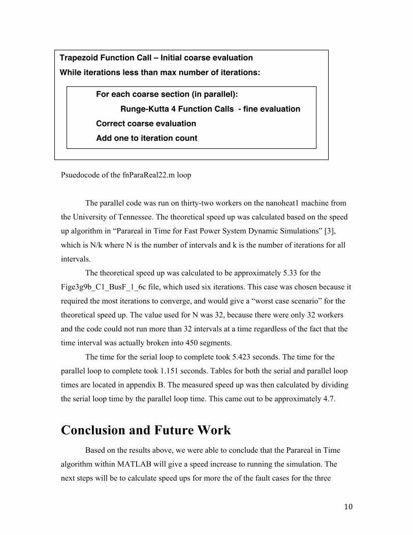
For the three generator and nine bus system, the section of code that iterates over
the coarse sections to solve the RK4 function uses a regular for loop for the serial code,
the fnParaReal22.m file. Psuedocode is displayed in the box below. To implement the
Parareal in Time Algorithm correctly, the for loop was replaced with a parfor loop, and
many of the data structures were rearranged to meet the requirements for running in
parallel (done by Aleksandar Dimitrovski).
10
Psuedocode of the fnParaReal22.m loop
The parallel code was run on thirty-two workers on the nanoheat1 machine from
the University of Tennessee. The theoretical speed up was calculated based on the speed
up algorithm in “Parareal in Time for Fast Power System Dynamic Simulations” [3],
which is N/k where N is the number of intervals and k is the number of iterations for all
intervals.
The theoretical speed up was calculated to be approximately 5.33 for the
Fige3g9b_C1_BusF_1_6c file, which used six iterations. This case was chosen because it
required the most iterations to converge, and would give a “worst case scenario” for the
theoretical speed up. The value used for N was 32, because there were only 32 workers
and the code could not run more than 32 intervals at a time regardless of the fact that the
time interval was actually broken into 450 segments.
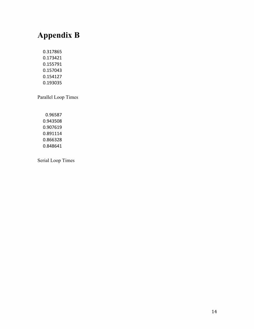
The time for the serial loop to complete took 5.423 seconds. The time for the
parallel loop to complete took 1.151 seconds. Tables for both the serial and parallel loop
times are located in appendix B. The measured speed up was then calculated by dividing
the serial loop time by the parallel loop time. This came out to be approximately 4.7.
Conclusion and Future Work Based on the results above, we were able to conclude that the Parareal in Time
algorithm within MATLAB will give a speed increase to running the simulation. The
next steps will be to calculate speed ups for more the of the fault cases for the three
For each coarse section (in parallel):
Runge-Kutta 4 Function Calls - fine evaluation
Correct coarse evaluation
Add one to iteration count
Trapezoid Function Call – Initial coarse evaluation
While iterations less than max number of iterations:

11
generator and nine bus system and then run the simulation for large systems and see how
the speed up scales with the system. Once it has been determined that the speed up is
consistent across multiple systems, C, C++, or Fortran code should be written from
scratch. The new code would be more flexible with parallel implementation and code
optimization.
12
Appendix A [7]
MATPOWER Version 5.1, 20-Mar-2015 -- AC Power Flow (Newton) Newton's method power flow converged in 4 iterations. Converged in 0.13 seconds System Summary
How Many? How Much? P (MW) Q (Mvar)
Buses 10 Total Gen Capacity 820.0 -‐900.00 to 900.00
Generators 3 On-line Capacity 820.0 -‐900.00 to 900.00
Committed Gens 3 Generation (actual) 319.6 22.8 Loads 3 Load 315.0 115.0 Fixed 3 Fixed 315.0 115.0 Dispatchable 0 Dispatchable -‐0.0 of -‐0.0 -‐0.0 Shunts 0 Shunt (inj) -‐0.0 0.0 Branches 11 Losses (I^2 * Z) 4.64 48.38 Transformers 0 Branch Charging (inj) -‐ 140.5 Inter-ties 0 Total Inter-tie Flow 0.0 0.0 Areas 1
Minimum Maximum
Voltage Magnitude 0.996 p.u. @ bus 5 1.040 p.u. @ bus 1 Voltage Angle -‐3.99 deg @ bus 5 9.28 deg @ bus 2 P Losses (I^2*R) -‐ 2.30 MW @ line 5-‐7 Q Losses (I^2*X) -‐ 15.83 Mvar @ line 2-‐7
Bus Data
Voltage Generation Load Bus # Mag (pu) Ang (deg) P (MW) Q (MVAr) P (MW) Q (MVAr) 1 1.040 0.000 71.64 27.05 -‐ -‐ 2 1.025 9.280 163.00 6.65 -‐ -‐ 3 1.025 4.665 85.00 -‐10.86 -‐ -‐ 4 1.026 -‐2.217 -‐ -‐ -‐ -‐ 5 0.996 -‐3.989 -‐ -‐ 125.00 50.00 6 1.013 -‐3.687 -‐ -‐ 90.00 30.00 7 1.026 3.720 -‐ -‐ -‐ -‐ 8 1.016 0.728 -‐ -‐ 100.00 35.00 9 1.032 1.967 -‐ -‐ -‐ -‐ 10 1.024 6.499 -‐ -‐ -‐ -‐
13
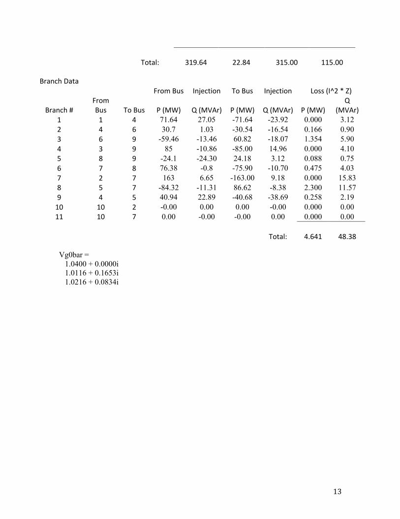
Total: 319.64 22.84 315.00 115.00
Branch Data
From Bus Injection To Bus Injection Loss (I^2 * Z)
Branch # From Bus To Bus P (MW) Q (MVAr) P (MW) Q (MVAr) P (MW)
Q (MVAr)
1 1 4 71.64 27.05 -71.64 -23.92 0.000 3.12 2 4 6 30.7 1.03 -30.54 -16.54 0.166 0.90 3 6 9 -59.46 -13.46 60.82 -18.07 1.354 5.90 4 3 9 85 -10.86 -85.00 14.96 0.000 4.10 5 8 9 -24.1 -24.30 24.18 3.12 0.088 0.75 6 7 8 76.38 -0.8 -75.90 -10.70 0.475 4.03 7 2 7 163 6.65 -163.00 9.18 0.000 15.83 8 5 7 -84.32 -11.31 86.62 -8.38 2.300 11.57 9 4 5 40.94 22.89 -40.68 -38.69 0.258 2.19 10 10 2 -0.00 0.00 0.00 -0.00 0.000 0.00 11 10 7 0.00 -0.00 -0.00 0.00 0.000 0.00
Total: 4.641 48.38
Vg0bar = 1.0400 + 0.0000i 1.0116 + 0.1653i 1.0216 + 0.0834i
14
Appendix B
0.317865 0.173421 0.155791 0.157043 0.154127 0.193035
Parallel Loop Times
0.96587 0.943508 0.907619 0.891114 0.866328 0.848641
Serial Loop Times
15
Sources [1] Dictionary.com. Dictionary.com. Web. 6 Aug. 2015.
[2] Gurrala, Gurunath. "Power System Parallel Dynamic Simulation Framework for Real
Time Wide-Area Protection and Control."
[3] Gurrala, Gurunath, Aleksandar Dimitrovski, Pannala Sreekanth, Srdjan Simunovic,
and Michael Starke. "Parareal in Time for Fast Power System Dynamic Simulations."
[4] Idema, Reijer, and Domenico Lahaye. Computational Methods in Power System
Analysis. Delft: Atlantis, 2014. Print.
[5] McCalley, James. The Power Flow Problem. Ames. Print.
[6] Meier, Alexandra Von. Electric Power Systems A Conceptual Introduction. Hoboken,
N.J.: IEEE :, 2006. Print.
[7] Zimmerman, Ray D., and Carlos E. Murillo-Sanchez. MatPower. Computer software.
MatPower. Vers. 5.1. N.p., 20 Apr. 2015. Web.
<http://www.pserc.cornell.edu//matpower/>.