PostGISTips for Power Users

pramsey@opengeo.org

PostGIS and PostgreSQL can be intimidating, and there are a lot of things to learn!There are hundreds of functions available, and it is hard to get past simple things like ST_Intersects and ST_DWithin to the next level.But once you get to the next level, youʼll find that PostGIS is as powerful (or more) than many desktop GIS systems.

My son suggested the following topical breakdown.

• Putting things together

• Taking things apart

• Fixing broken things

• Copying other people

• Playing with balls

• Going really fast

Putting things together

ST_GeomFromText( 'POINT('||x||' '||y||')')

We may only be able to cover the first few in the time available.

There are lots of functions that build new geometries from parts

The standard constructors you might see are ST_GeometryFromText() or perhaps one of the new ones like ST_GeometryFromGML(). Because they read from text, they lead to ugly statements like this one.

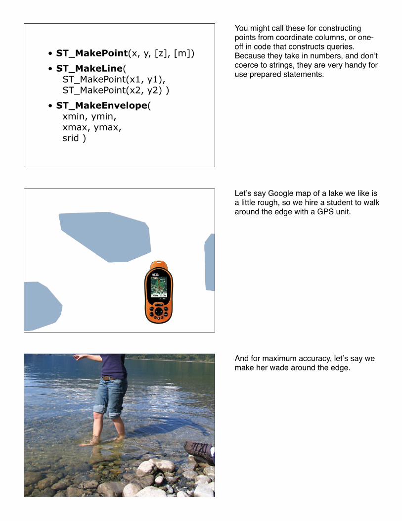
• ST_MakePoint(x, y, [z], [m])

• ST_MakeLine( ST_MakePoint(x1, y1), ST_MakePoint(x2, y2) )

• ST_MakeEnvelope( xmin, ymin, xmax, ymax, srid )

You might call these for constructing points from coordinate columns, or one-off in code that constructs queries. Because they take in numbers, and donʼt coerce to strings, they are very handy for use prepared statements.

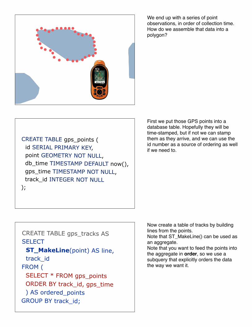
Letʼs say Google map of a lake we like is a little rough, so we hire a student to walk around the edge with a GPS unit.

And for maximum accuracy, letʼs say we make her wade around the edge.

CREATE TABLE gps_points ( id SERIAL PRIMARY KEY, point GEOMETRY NOT NULL, db_time TIMESTAMP DEFAULT now(), gps_time TIMESTAMP NOT NULL, track_id INTEGER NOT NULL);

CREATE TABLE gps_tracks AS SELECT ST_MakeLine(point) AS line, track_id FROM ( SELECT * FROM gps_points ORDER BY track_id, gps_time ) AS ordered_points GROUP BY track_id;

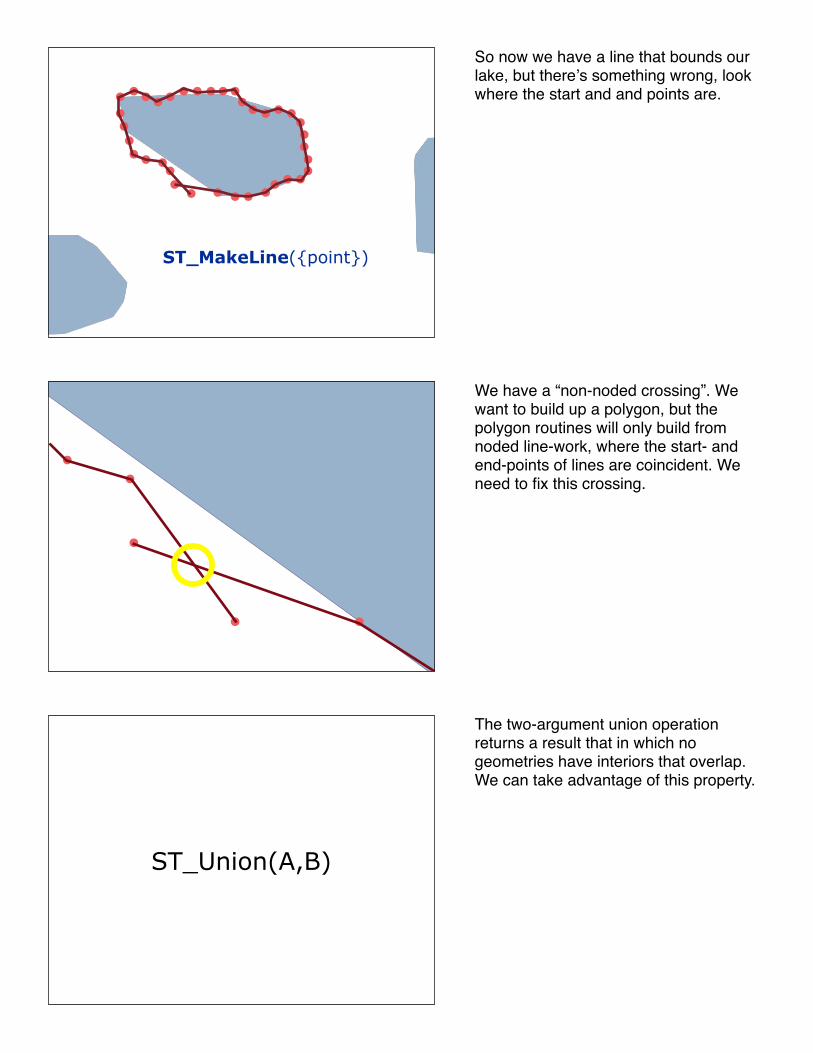
We end up with a series of point observations, in order of collection time. How do we assemble that data into a polygon?

First we put those GPS points into a database table. Hopefully they will be time-stamped, but if not we can stamp them as they arrive, and we can use the id number as a source of ordering as well if we need to.

Now create a table of tracks by building lines from the points.Note that ST_MakeLine() can be used as an aggregate.Note that you want to feed the points into the aggregate in order, so we use a subquery that explicitly orders the data the way we want it.

ST_MakeLine({point})

ST_Union(A,B)

So now we have a line that bounds our lake, but thereʼs something wrong, look where the start and and points are.

We have a “non-noded crossing”. We want to build up a polygon, but the polygon routines will only build from noded line-work, where the start- and end-points of lines are coincident. We need to fix this crossing.

The two-argument union operation returns a result that in which no geometries have interiors that overlap. We can take advantage of this property.

ST_Union(A,B)

UPDATE gps_tracksSET line = ST_Union(

line, ‘LINESTRING EMPTY’

)

CREATE TABLE gps_lakes AS SELECT ST_BuildArea(line) AS lake, track_id FROM gps_tracks;

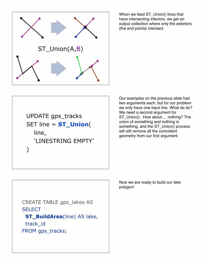
When we feed ST_Union() lines that have intersecting interiors, we get an output collection where only the exteriors (the end points) intersect.

Our examples on the previous slide had two arguments each, but for our problem we only have one input line. What do do?We need a second argument for ST_Union(). How about ... nothing? The union of something and nothing is something, and the ST_Union() process will still remove all the coincident geometry from our first argument.

Now we are ready to build our lake polygon!

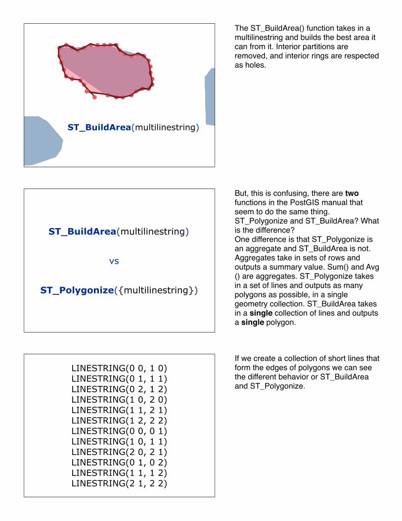
ST_BuildArea(multilinestring)

ST_BuildArea(multilinestring)

ST_Polygonize({multilinestring})

vs

LINESTRING(0 0, 1 0)LINESTRING(0 1, 1 1)LINESTRING(0 2, 1 2)LINESTRING(1 0, 2 0)LINESTRING(1 1, 2 1)LINESTRING(1 2, 2 2)LINESTRING(0 0, 0 1)LINESTRING(1 0, 1 1)LINESTRING(2 0, 2 1)LINESTRING(0 1, 0 2)LINESTRING(1 1, 1 2)LINESTRING(2 1, 2 2)

The ST_BuildArea() function takes in a multilinestring and builds the best area it can from it. Interior partitions are removed, and interior rings are respected as holes.

But, this is confusing, there are two functions in the PostGIS manual that seem to do the same thing. ST_Polygonize and ST_BuildArea? What is the difference?One difference is that ST_Polygonize is an aggregate and ST_BuildArea is not. Aggregates take in sets of rows and outputs a summary value. Sum() and Avg() are aggregates. ST_Polygonize takes in a set of lines and outputs as many polygons as possible, in a single geometry collection. ST_BuildArea takes in a single collection of lines and outputs a single polygon.

If we create a collection of short lines that form the edges of polygons we can see the different behavior or ST_BuildArea and ST_Polygonize.

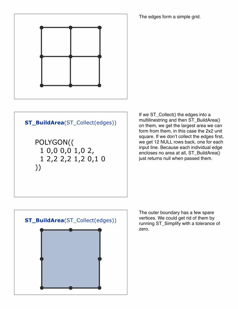
ST_BuildArea(ST_Collect(edges))

POLYGON(( 1 0,0 0,0 1,0 2, 1 2,2 2,2 1,2 0,1 0))

ST_BuildArea(ST_Collect(edges))

The edges form a simple grid.

If we ST_Collect() the edges into a multilinestring and then ST_BuildArea() on them, we get the largest area we can form from them, in this case the 2x2 unit square. If we donʼt collect the edges first, we get 12 NULL rows back, one for each input line. Because each individual edge encloses no area at all, ST_BuildArea() just returns null when passed them.

The outer boundary has a few spare vertices. We could get rid of them by running ST_Simplify with a tolerance of zero.

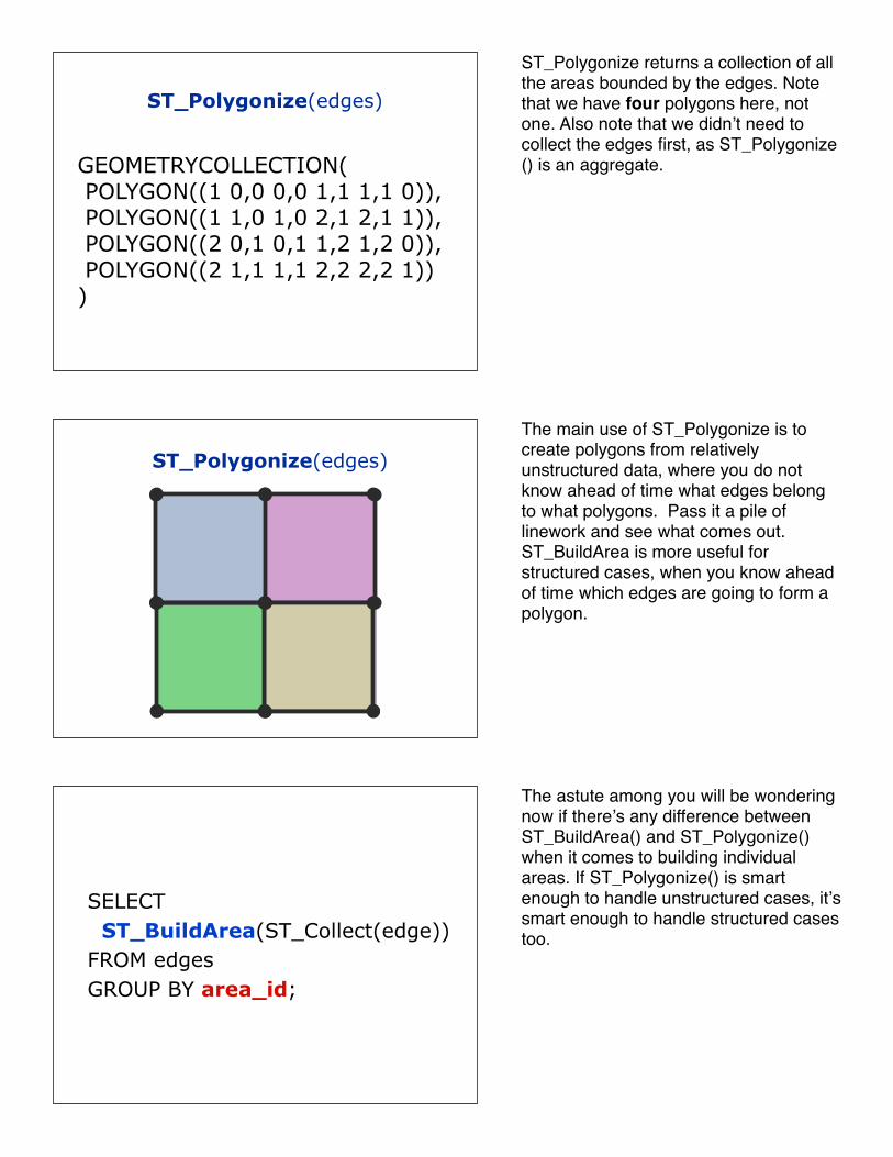
GEOMETRYCOLLECTION( POLYGON((1 0,0 0,0 1,1 1,1 0)), POLYGON((1 1,0 1,0 2,1 2,1 1)), POLYGON((2 0,1 0,1 1,2 1,2 0)), POLYGON((2 1,1 1,1 2,2 2,2 1)))

ST_Polygonize(edges)

ST_Polygonize(edges)

SELECT ST_BuildArea(ST_Collect(edge)) FROM edges GROUP BY area_id;

ST_Polygonize returns a collection of all the areas bounded by the edges. Note that we have four polygons here, not one. Also note that we didnʼt need to collect the edges first, as ST_Polygonize() is an aggregate.

The main use of ST_Polygonize is to create polygons from relatively unstructured data, where you do not know ahead of time what edges belong to what polygons. Pass it a pile of linework and see what comes out.ST_BuildArea is more useful for structured cases, when you know ahead of time which edges are going to form a polygon.

The astute among you will be wondering now if thereʼs any difference between ST_BuildArea() and ST_Polygonize() when it comes to building individual areas. If ST_Polygonize() is smart enough to handle unstructured cases, itʼs smart enough to handle structured cases too.

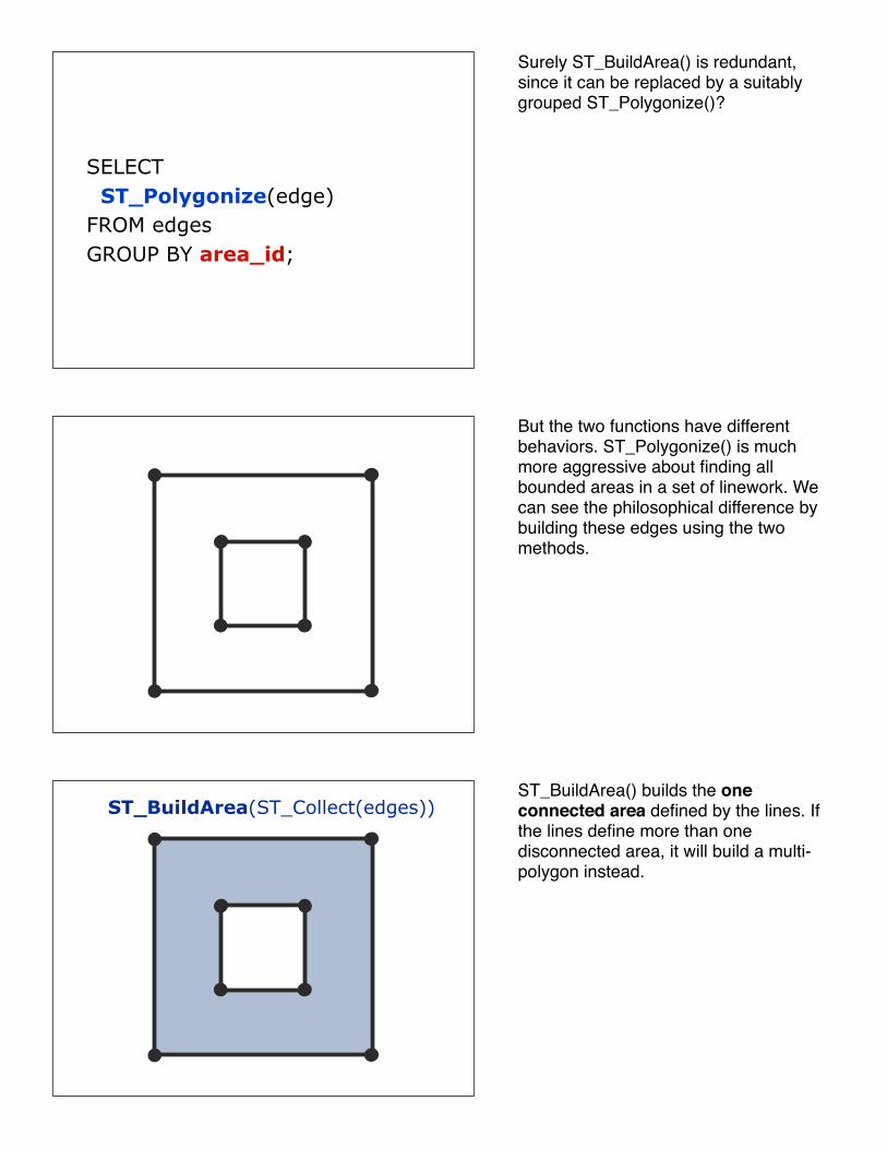
SELECT ST_Polygonize(edge) FROM edges GROUP BY area_id;

ST_BuildArea(ST_Collect(edges))

Surely ST_BuildArea() is redundant, since it can be replaced by a suitably grouped ST_Polygonize()?

But the two functions have different behaviors. ST_Polygonize() is much more aggressive about finding all bounded areas in a set of linework. We can see the philosophical difference by building these edges using the two methods.

ST_BuildArea() builds the one connected area defined by the lines. If the lines define more than one disconnected area, it will build a multi-polygon instead.

ST_Polygonize(edges)

Taking things apart

geom name

GEOMETRYCOLLECTION( POINT(0 0), POINT(1 1))

Paul

geom name

POINT(0 0) Paul

POINT(1 1) Paul

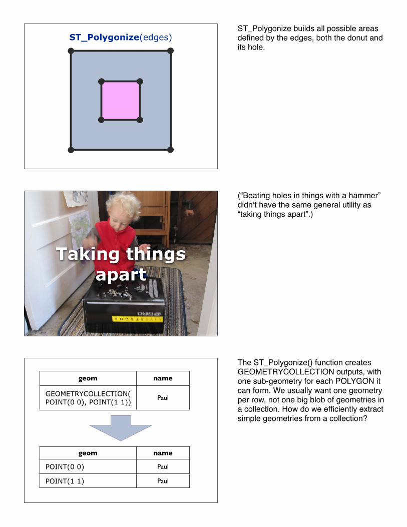
ST_Polygonize builds all possible areas defined by the edges, both the donut and its hole.

(“Beating holes in things with a hammer” didnʼt have the same general utility as “taking things apart”.)

The ST_Polygonize() function creates GEOMETRYCOLLECTION outputs, with one sub-geometry for each POLYGON it can form. We usually want one geometry per row, not one big blob of geometries in a collection. How do we efficiently extract simple geometries from a collection?

ST_GeometryN(collection, n)

ST_Dump(collection)

vs

SELECT ST_GeometryN(geom,1), nameFROM the_table;

st_geometryn name

POINT(0 0) Paul

SELECT ST_GeometryN(geom, generate_series( 1, ST_NumGeometries(geom))), nameFROM the_table;

st_geometryn name

POINT(0 0) Paul

POINT(1 1) Paul

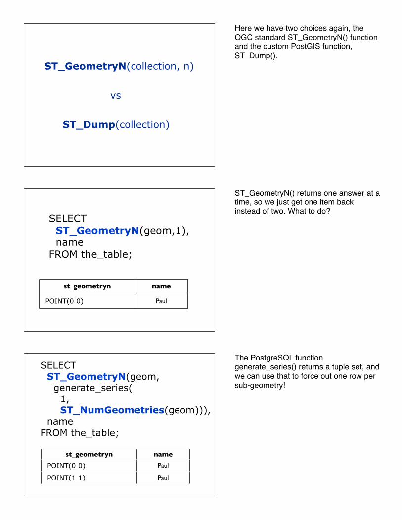
Here we have two choices again, the OGC standard ST_GeometryN() function and the custom PostGIS function, ST_Dump().

ST_GeometryN() returns one answer at a time, so we just get one item back instead of two. What to do?

The PostgreSQL function generate_series() returns a tuple set, and we can use that to force out one row per sub-geometry!

SELECT ST_Dump(geom), nameFROM the_table;

st_dump name

({1},0101...000000) Paul

({2},0101...000000) Paul

geometry_dump [ path: array(int) geom: geometry]

SELECT (ST_Dump(geom)).geom, nameFROM the_table;

geom name

POINT(0 0) Paul

POINT(1 1) Paul

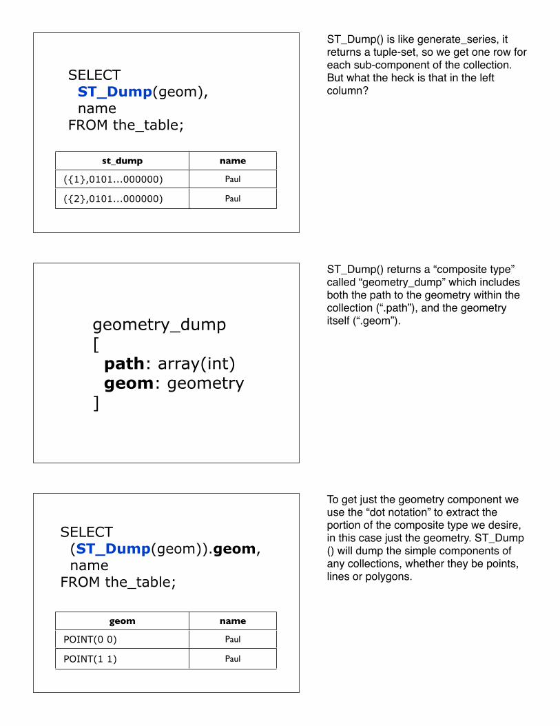
ST_Dump() is like generate_series, it returns a tuple-set, so we get one row for each sub-component of the collection. But what the heck is that in the left column?

ST_Dump() returns a “composite type” called “geometry_dump” which includes both the path to the geometry within the collection (“.path”), and the geometry itself (“.geom”).

To get just the geometry component we use the “dot notation” to extract the portion of the composite type we desire, in this case just the geometry. ST_Dump() will dump the simple components of any collections, whether they be points, lines or polygons.

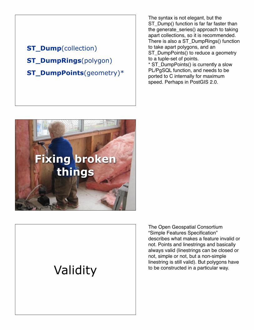
ST_Dump(collection)

ST_DumpRings(polygon)

ST_DumpPoints(geometry)*

Fixing broken things

Validity

The syntax is not elegant, but the ST_Dump() function is far far faster than the generate_series() approach to taking apart collections, so it is recommended.There is also a ST_DumpRings() function to take apart polygons, and an ST_DumpPoints() to reduce a geometry to a tuple-set of points.* ST_DumpPoints() is currently a slow PL/PgSQL function, and needs to be ported to C internally for maximum speed. Perhaps in PostGIS 2.0.

The Open Geospatial Consortium “Simple Features Specification” describes what makes a feature invalid or not. Points and linestrings and basically always valid (linestrings can be closed or not, simple or not, but a non-simple linestring is still valid). But polygons have to be constructed in a particular way.

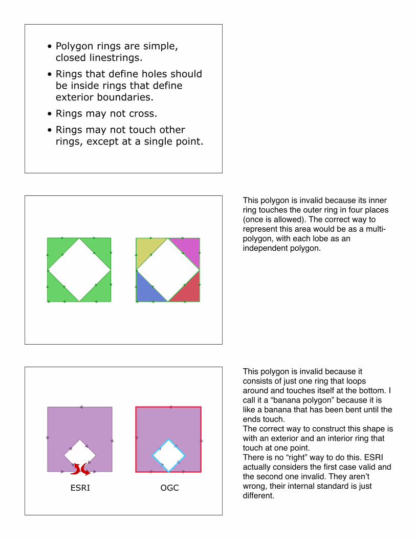
• Polygon rings are simple, closed linestrings.

• Rings that define holes should be inside rings that define exterior boundaries.

• Rings may not cross.

• Rings may not touch other rings, except at a single point.

ESRI OGC

This polygon is invalid because its inner ring touches the outer ring in four places (once is allowed). The correct way to represent this area would be as a multi-polygon, with each lobe as an independent polygon.

This polygon is invalid because it consists of just one ring that loops around and touches itself at the bottom. I call it a “banana polygon” because it is like a banana that has been bent until the ends touch. The correct way to construct this shape is with an exterior and an interior ring that touch at one point. There is no “right” way to do this. ESRI actually considers the first case valid and the second one invalid. They arenʼt wrong, their internal standard is just different.

SELECT ST_Area( );

0

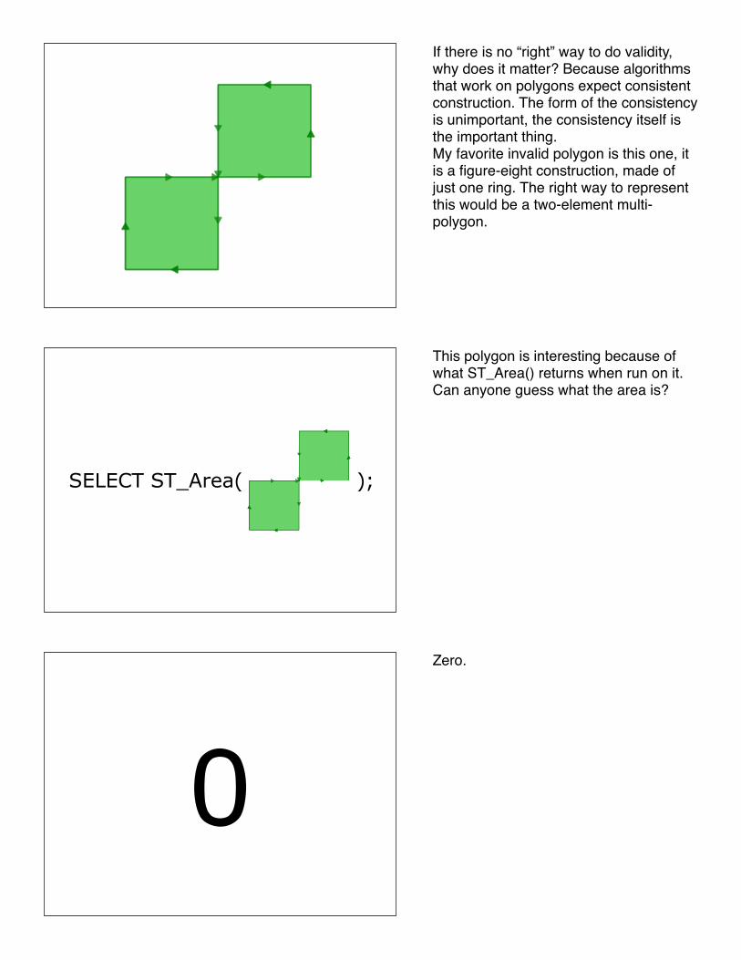
If there is no “right” way to do validity, why does it matter? Because algorithms that work on polygons expect consistent construction. The form of the consistency is unimportant, the consistency itself is the important thing.My favorite invalid polygon is this one, it is a figure-eight construction, made of just one ring. The right way to represent this would be a two-element multi-polygon.

This polygon is interesting because of what ST_Area() returns when run on it.Can anyone guess what the area is?

Zero.

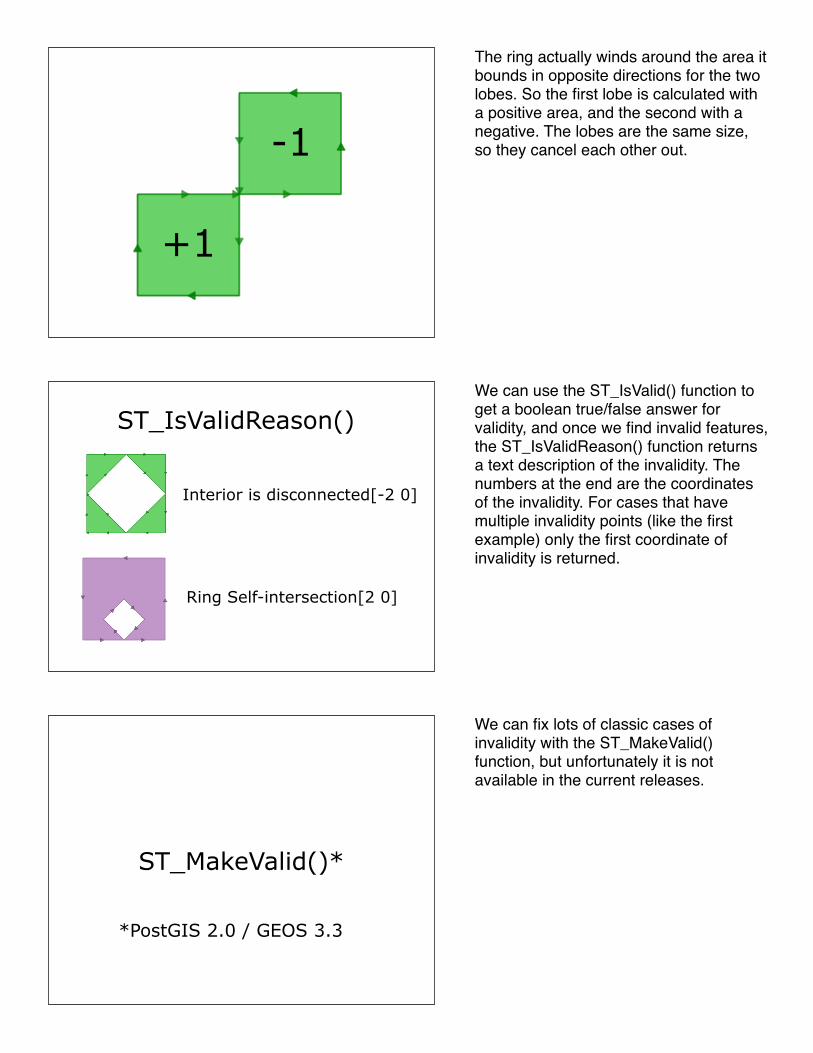
+1

-1

ST_IsValidReason()

Interior is disconnected[-2 0]

Ring Self-intersection[2 0]

ST_MakeValid()*

*PostGIS 2.0 / GEOS 3.3

The ring actually winds around the area it bounds in opposite directions for the two lobes. So the first lobe is calculated with a positive area, and the second with a negative. The lobes are the same size, so they cancel each other out.

We can use the ST_IsValid() function to get a boolean true/false answer for validity, and once we find invalid features, the ST_IsValidReason() function returns a text description of the invalidity. The numbers at the end are the coordinates of the invalidity. For cases that have multiple invalidity points (like the first example) only the first coordinate of invalidity is returned.

We can fix lots of classic cases of invalidity with the ST_MakeValid() function, but unfortunately it is not available in the current releases.

ST_Buffer(geom, 0.0)

ST_Buffer(geom, 0.0)

ST_Buffer(geom, 0.0)

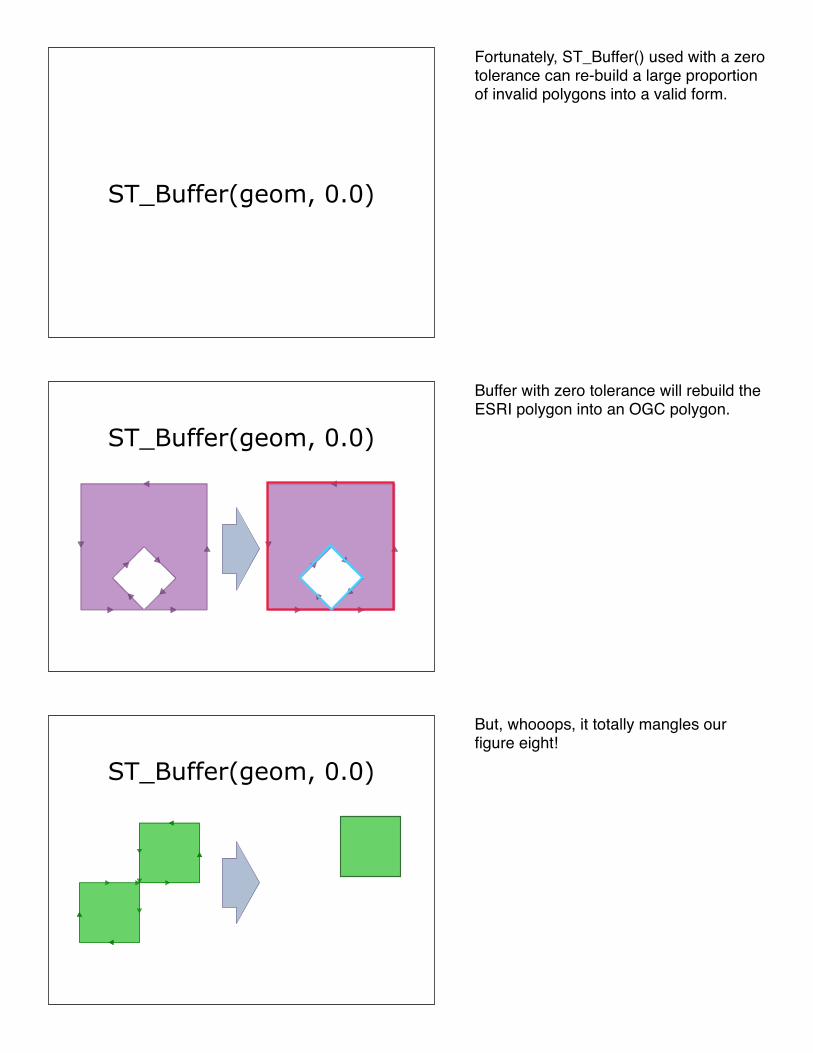
Fortunately, ST_Buffer() used with a zero tolerance can re-build a large proportion of invalid polygons into a valid form.

Buffer with zero tolerance will rebuild the ESRI polygon into an OGC polygon.

But, whooops, it totally mangles our figure eight!

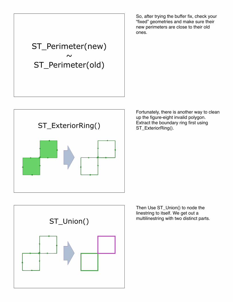
ST_Perimeter(new)~

ST_Perimeter(old)

ST_ExteriorRing()

ST_Union()

So, after trying the buffer fix, check your “fixed” geometries and make sure their new perimeters are close to their old ones.

Fortunately, there is another way to clean up the figure-eight invalid polygon.Extract the boundary ring first using ST_ExteriorRing().

Then Use ST_Union() to node the linestring to itself. We get out a multilinestring with two distinct parts.

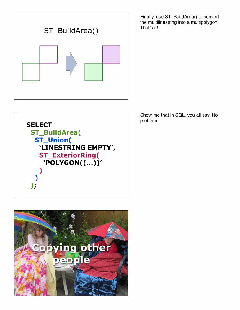
ST_BuildArea()

SELECT ST_BuildArea( ST_Union( ‘LINESTRING EMPTY’, ST_ExteriorRing( ‘POLYGON((...))’ ) ) );

Copying other people

Finally, use ST_BuildArea() to convert the multilinestring into a multipolygon. Thatʼs it!

Show me that in SQL, you all say. No problem!

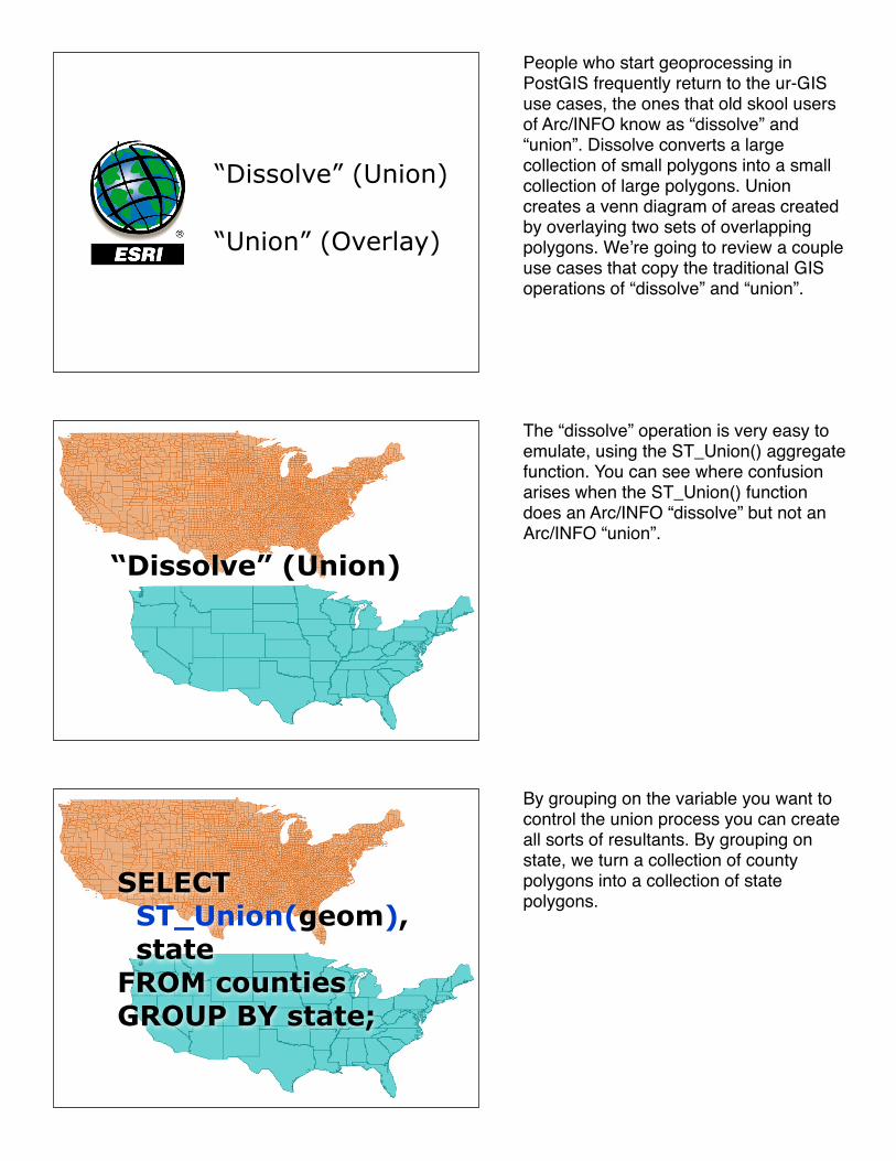
“Dissolve” (Union)

“Union” (Overlay)

“Dissolve” (Union)

SELECT ST_Union(geom), stateFROM countiesGROUP BY state;

People who start geoprocessing in PostGIS frequently return to the ur-GIS use cases, the ones that old skool users of Arc/INFO know as “dissolve” and “union”. Dissolve converts a large collection of small polygons into a small collection of large polygons. Union creates a venn diagram of areas created by overlaying two sets of overlapping polygons. Weʼre going to review a couple use cases that copy the traditional GIS operations of “dissolve” and “union”.

The “dissolve” operation is very easy to emulate, using the ST_Union() aggregate function. You can see where confusion arises when the ST_Union() function does an Arc/INFO “dissolve” but not an Arc/INFO “union”.

By grouping on the variable you want to control the union process you can create all sorts of resultants. By grouping on state, we turn a collection of county polygons into a collection of state polygons.

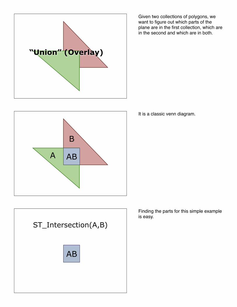
“Union” (Overlay)

A

B

AB

AB

ST_Intersection(A,B)

Given two collections of polygons, we want to figure out which parts of the plane are in the first collection, which are in the second and which are in both.

It is a classic venn diagram.

Finding the parts for this simple example is easy.

A

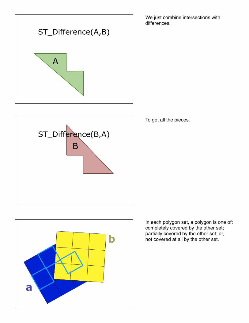
ST_Difference(A,B)

ST_Difference(B,A)

B

a

b

We just combine intersections with differences.

To get all the pieces.

In each polygon set, a polygon is one of:completely covered by the other set;partially covered by the other set; or,not covered at all by the other set.

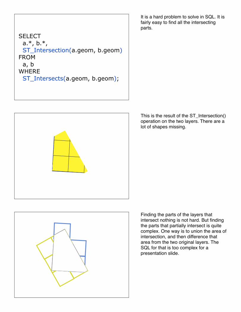
SELECT a.*, b.*, ST_Intersection(a.geom, b.geom)FROM a, bWHERE ST_Intersects(a.geom, b.geom);

It is a hard problem to solve in SQL. It is fairly easy to find all the intersecting parts.

This is the result of the ST_Intersection() operation on the two layers. There are a lot of shapes missing.

Finding the parts of the layers that intersect nothing is not hard. But finding the parts that partially intersect is quite complex. One way is to union the area of intersection, and then difference that area from the two original layers. The SQL for that is too complex for a presentation slide.

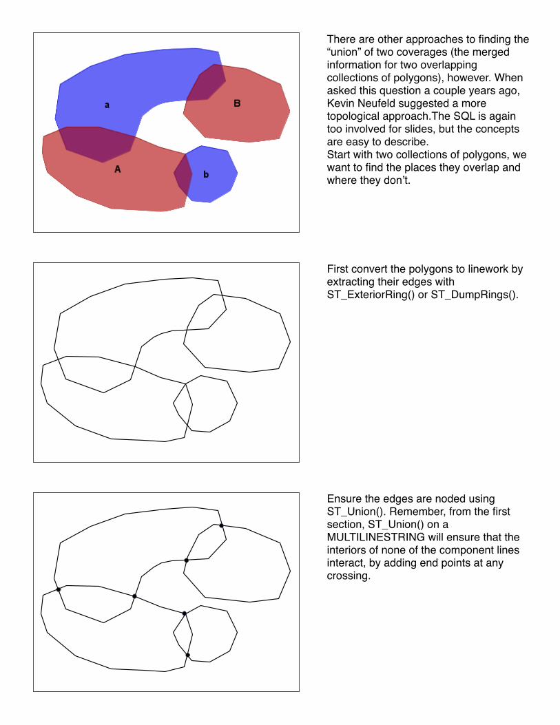
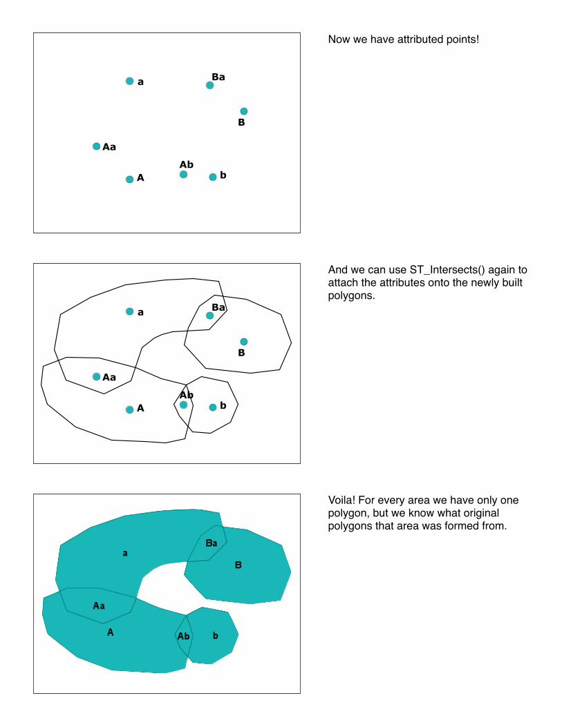
There are other approaches to finding the “union” of two coverages (the merged information for two overlapping collections of polygons), however. When asked this question a couple years ago, Kevin Neufeld suggested a more topological approach.The SQL is again too involved for slides, but the concepts are easy to describe.Start with two collections of polygons, we want to find the places they overlap and where they donʼt.

First convert the polygons to linework by extracting their edges with ST_ExteriorRing() or ST_DumpRings().

Ensure the edges are noded using ST_Union(). Remember, from the first section, ST_Union() on a MULTILINESTRING will ensure that the interiors of none of the component lines interact, by adding end points at any crossing.

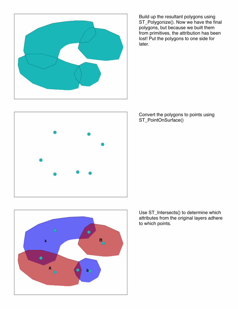
Build up the resultant polygons using ST_Polygonize(). Now we have the final polygons, but because we built them from primitives, the attribution has been lost! Put the polygons to one side for later.

Convert the polygons to points using ST_PointOnSurface()

Use ST_Intersects() to determine which attributes from the original layers adhere to which points.

A

Aa

a

bAb

B

Ba

A

Aa

a

bAb

B

Ba

Now we have attributed points!

And we can use ST_Intersects() again to attach the attributes onto the newly built polygons.

Voila! For every area we have only one polygon, but we know what original polygons that area was formed from.

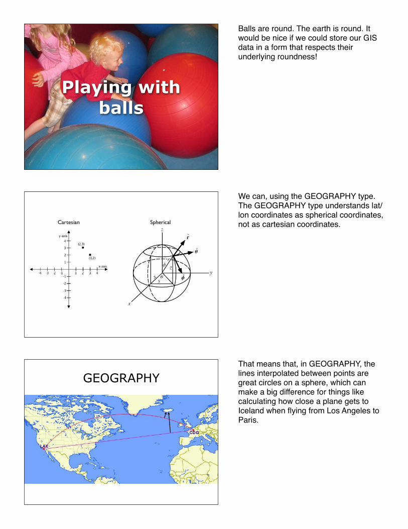
Playing with balls

GEOGRAPHY

Balls are round. The earth is round. It would be nice if we could store our GIS data in a form that respects their underlying roundness!

We can, using the GEOGRAPHY type. The GEOGRAPHY type understands lat/lon coordinates as spherical coordinates, not as cartesian coordinates.

That means that, in GEOGRAPHY, the lines interpolated between points are great circles on a sphere, which can make a big difference for things like calculating how close a plane gets to Iceland when flying from Los Angeles to Paris.

• Index over sphere

• Calculate over poles / dateline

• Precise calculations on spheroid

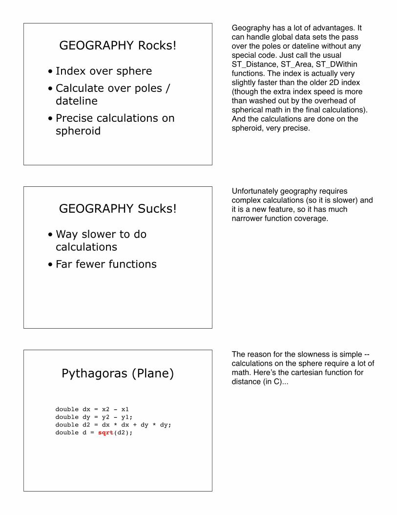
GEOGRAPHY Rocks!

• Way slower to do calculations

• Far fewer functions

GEOGRAPHY Sucks!

double dx = x2 - x1double dy = y2 - y1;double d2 = dx * dx + dy * dy;double d = sqrt(d2);

Pythagoras (Plane)

Geography has a lot of advantages. It can handle global data sets the pass over the poles or dateline without any special code. Just call the usual ST_Distance, ST_Area, ST_DWithin functions. The index is actually very slightly faster than the older 2D index (though the extra index speed is more than washed out by the overhead of spherical math in the final calculations). And the calculations are done on the spheroid, very precise.

Unfortunately geography requires complex calculations (so it is slower) and it is a new feature, so it has much narrower function coverage.

The reason for the slowness is simple -- calculations on the sphere require a lot of math. Hereʼs the cartesian function for distance (in C)...

double R = 6371000; /* meters */double d_lat = lat2-lat1; /* radians */double d_lon = lon2-lon1; /* radians */double a = sin(d_lat/2) * sin(d_lat/2) +        cos(lat1) * cos(lat2) *         sin(d_lon/2) * sin(d_lon/2); double c = 2 * atan2(sqrt(a), sqrt(1-a)); double d = R * c;

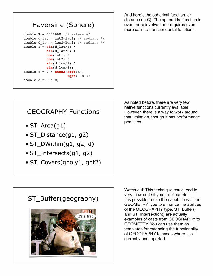
Haversine (Sphere)

• ST_Area(g1)

• ST_Distance(g1, g2)

• ST_DWithin(g1, g2, d)

• ST_Intersects(g1, g2)

• ST_Covers(gpoly1, gpt2)

GEOGRAPHY Functions

ST_Buffer(geography)

And hereʼs the spherical function for distance (in C). The spheroidal function is even more involved and requires even more calls to transcendental functions.

As noted before, there are very few native functions currently available. However, there is a way to work around that limitation, though it has performance penalties.

Watch out! This technique could lead to very slow code if you arenʼt careful!It is possible to use the capabilities of the GEOMETRY type to enhance the abilities of the GEOGRAPHY type. ST_Buffer() and ST_Intersection() are actually examples of casts from GEOGRAPHY to GEOMETRY. You can use them as templates for extending the functionality of GEOGRAPHY to cases where it is currently unsupported.

ST_Transform( _ST_BestSRID($1) ),

ST_Buffer( $2),

ST_Transform( 4326)

SELECT geography( )

geometry($1),

ST_Buffer(geography)

_ST_BestSRID(geog)

_ST_BestSRID(geog)

_ST_BestSRID(geog1, geog2)

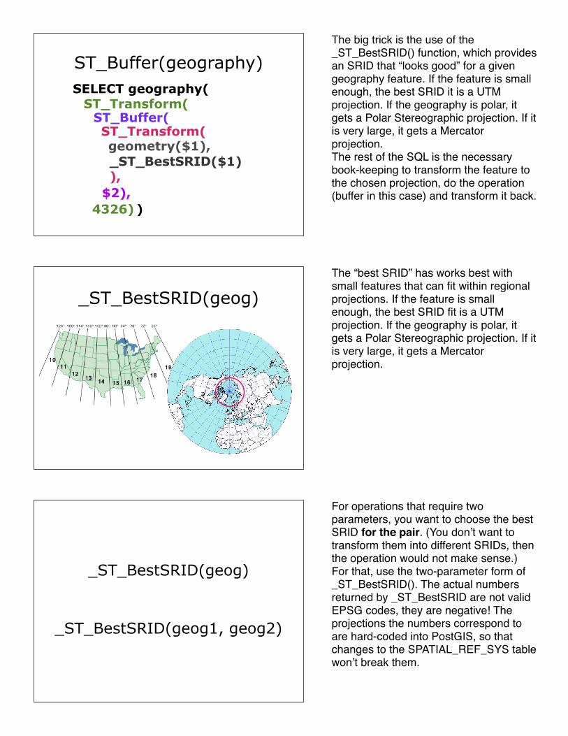
The big trick is the use of the _ST_BestSRID() function, which provides an SRID that “looks good” for a given geography feature. If the feature is small enough, the best SRID it is a UTM projection. If the geography is polar, it gets a Polar Stereographic projection. If it is very large, it gets a Mercator projection.The rest of the SQL is the necessary book-keeping to transform the feature to the chosen projection, do the operation (buffer in this case) and transform it back.

The “best SRID” has works best with small features that can fit within regional projections. If the feature is small enough, the best SRID fit is a UTM projection. If the geography is polar, it gets a Polar Stereographic projection. If it is very large, it gets a Mercator projection.

For operations that require two parameters, you want to choose the best SRID for the pair. (You donʼt want to transform them into different SRIDs, then the operation would not make sense.) For that, use the two-parameter form of _ST_BestSRID(). The actual numbers returned by _ST_BestSRID are not valid EPSG codes, they are negative! The projections the numbers correspond to are hard-coded into PostGIS, so that changes to the SPATIAL_REF_SYS table wonʼt break them.

SELECT geography( ST_StartPoint( geometry($1) ))

ST_StartPoint(geography)

Going really fast

CREATE INDEX your_geoindexON your_table

USING GIST (your_geocolumn);

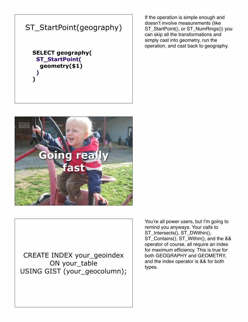
If the operation is simple enough and doesnʼt involve measurements (like ST_StartPoint(), or ST_NumRings()) you can skip all the transformations and simply cast into geometry, run the operation, and cast back to geography.

Youʼre all power users, but Iʼm going to remind you anyways. Your calls to ST_Intersects(), ST_DWithin(), ST_Contains(), ST_Within(), and the && operator of course, all require an index for maximum efficiency. This is true for both GEOGRAPHY and GEOMETRY, and the index operator is && for both types.

Server Memory

OS shared_buffers *_mem

15% 65% 20%

Run-time Parameters!

• SET work_mem TO 2GB;

• SET maintenance_work_mem TO 1GB;

• SET client_min_messages TO DEBUG;

Spend some money

• I/O is biggest bottleneck

• Invest in

• Great file system

• Good memory

• Adequate CPU(s)

Do not starve your system of memory. The defaults are low low low!Go into postgresql.conf and set up PostgreSQL to make good use of your server RAM. Assuming you have a dedicated database server, these are simple rules of thumb. You have to re-start the database for the shared_buffers parameter to take effect.

Some of the memory parameters are actually run-time! This is hugely powerful. Building an index on a 100M record table? Increase your work_mem to 3GB and watch your index build time drop 75%. Vacuuming after a big update? Increase your maintenance_work_mem and watch the process zip along. Doing some coding on PL/PgSQL functions? Turn up client_min_messages to ʻDEBUGʼ and just your session will see the extra debugging information you need to work.

Once the size of your database is larger than your main memory, you are going to bottleneck at the I/O bus. Get a RAID10 array, and a good quality controller to back it. (Incidentally, one of the reasons cloud PostgreSQL is dicey is because the I/O on the cloud systems is slow and flakey.) Get as much memory as you can -- the more things that are in memory cache, the faster things go. A “good enough” CPU (or four) will do.

Clustering

Clustering

Cluster on R-Tree

CLUSTER your_table USING your_geoindex;

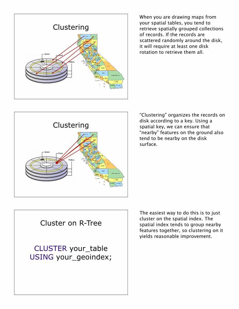
When you are drawing maps from your spatial tables, you tend to retrieve spatially grouped collections of records. If the records are scattered randomly around the disk, it will require at least one disk rotation to retrieve them all.

“Clustering” organizes the records on disk according to a key. Using a spatial key, we can ensure that “nearby” features on the ground also tend to be nearby on the disk surface.

The easiest way to do this is to just cluster on the spatial index. The spatial index tends to group nearby features together, so clustering on it yields reasonable improvement.

Cluster on GeoHash

CREATE INDEX your_geohash_index ON your_table (ST_GeoHash(your_geocolumn));

CLUSTER your_table USING your_geohash_index;

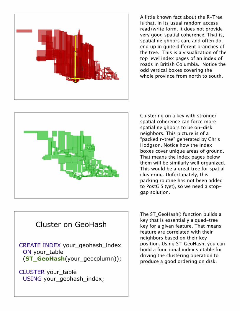
A little known fact about the R-Tree is that, in its usual random access read/write form, it does not provide very good spatial coherence. That is, spatial neighbors can, and often do, end up in quite different branches of the tree. This is a visualization of the top level index pages of an index of roads in British Columbia. Notice the odd vertical boxes covering the whole province from north to south.

Clustering on a key with stronger spatial coherence can force more spatial neighbors to be on-disk neighbors. This picture is of a “packed r-tree” generated by Chris Hodgson. Notice how the index boxes cover unique areas of ground. That means the index pages below them will be similarly well organized. This would be a great tree for spatial clustering. Unfortunately, this packing routine has not been added to PostGIS (yet), so we need a stop-gap solution.

The ST_GeoHash() function builds a key that is essentially a quad-tree key for a given feature. That means feature are correlated with their neighbors based on their key position. Using ST_GeoHash, you can build a functional index suitable for driving the clustering operation to produce a good ordering on disk.

Stay curious

• Join the mailing listhttp://postgis.org/mailman/listinfo/postgis-users

• Read the wiki! And add stuff!http://trac.osgeo.org/postgis

• Buy the bookhttp://www.manning.com/obe/

• Read GIS StackExchangehttp://gis.stackexchange.com/

• Start using PL/R!http://www.joeconway.com/plr/

• Use R Geostatistics!http://geodacenter.asu.edu/r-spatial-projects

• Join IRC!irc://irc.freenode.net/postgis

• Use the sourcehttp://svn.osgeo.org/postgis/trunk/

PostGIS has gotten really huge! There is always more to learn!

Thanks

http://s3.opengeo.org/postgis-power.pdf

Thanks, from me and PT.

You can download the slides and notes for this talk from this URL.