GEOHORIZONS December 2007/5

Brief about the field and need for 4D Seismic

Based on 2D seismic data, the Neelam field wasmapped as two independent culminations and two exploratorywells, E1 on south and E2 on north, were drilled. Both turnedout to be prolific producers of Oil and Gas. Subsequentdrilling of another exploratory well E3 in-between E1 and E2,which falls in a saddle, also produced hydrocarbon. A 3Dsurvey was conducted in 1989, with a bin size of 12.5m X87.5m, to image the subsurface and the field was put onproduction since 1990. The structure map and the wells drilledare as shown in Fig.1. The base survey(89) due to its coarsebin size failed to image minor and subtle faults especiallythose which were aligned to cross line direction. These minorand subtle faults were in fact working as conduit for earlywater break through from injectors to producers. In order tohave a more detailed picture of the subsurface, it was decidedto re-shoot the area with smaller bin size of 12.5m X 37.5 m.The brief acquisition parameters are given in Table-1. Thefield reached its production peak in 1995 but soon theproduction steadily declined to one third and by the time therepeat survey was completed an estimated 16% of initial oilin place had been produced. Despite fall in production, itwas believed that the field had the potential to produce moreand the field was identified for the first offshore 4D seismicproject in India for reservoir surveillance and detailedsubsurface imaging. In order to understand the complexity, a

Post Stack 4D Seismic Data Conditioning, Matching and Validationto Map the Changes in Fluid Phase

Partha P.Mitra, J.V.S.S.N.Murty, B.S.Josyulu, Mohan Menon and Gautam Sen

Summary

4D seismic has emerged as a powerful reservoir surveillance tool to map the changes in fluid phaseswithin a reservoir in a producing field. Though it has worked excellently well in clastic reservoir, monitoringthe same within a carbonate reservoir in a producing field is still a challenging task as the Gassman's equation'doesn't predict the nature of velocity sensitivity to fluid change in most carbonate rocks'. Moreover thedifference in seismic signature due to hydrocarbon extraction is often buried within the background noise.Therefore, the success lies how well, one can preserve the subtle variations in the seismic signature throughproper conditioning, matching and subsequent validation before deciding about any investment propositionto improve the ultimate recovery from the field. The paper presents a post stack conditioning and equalizationof two 3D seismic surveys or in other words 4D seismic carried out over a field called Neelam in westernoffshore of India. The field produces from Eocene limestone which is affected by Karstification of differenttypes and of different degree. The initial or base survey was carried out before the commencement of productionin 1989 and the repeat survey was conducted after a time lapse of ten years. The field was initially developedwith peripheral water injection and had produced about 16% of initial oil in place by the time the repeat surveywas completed. The two survey parameters were different and basic processing of two vintages was carriedout by two different vendors. However, more or less the same processing sequences were followed. Variousinnovative methods for conditioning and equalization techniques were used to arrive at a most robustconditioned data. Individual as well as difference volumes were generated. At non reservoir level, the differenceseismic volume showed almost negligible difference and this led to a high level of confidence in mapping thechange in fluid phase within the reservoir. It has been concluded that the effect of Karstification has playedan important role in bringing out the seismic observables in time lapse datasets. The study has helped to mapthe areas of bypassed oil and also the areas affected by water flooding.

Fig. 1. Structure map of the field.

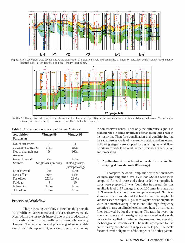
detailed core study, reprocessing of wire-line logs and specialprocessing of existing 3D seismic and 4D seismic were carriedout. The core & processed logs revealed the presence ofkarstification of varied intensity. The process of karstificationhas significantly contributed in porosity generation anddevelopment of the major hydrocarbon reserve and believedto be the major factor causing change in seismic signaturesduring production cycle. Fig.2 brings out two major geologicalprofiles one in NS and other one in EW direction depictingthe types of karst present within the reservoir and theirseverity.

GEOHORIZONS December 2007/6

Processing Workflow

The processing workflow is based on the principlethat the differential seismic signals of elapsed surveys mainlyoccur within the reservoir interval due to the production ofhydrocarbons and can be attributed to reservoir propertychanges. The acquisition and processing of seismic datashould ensure the repeatability of seismic character pertaining

to non-reservoir zones. Then only the difference signal canbe interpreted in terms amplitude of changes in fluid phase inthe reservoir. Therefore equalization and conditioning thedata at non-reservoir level is extremely critical and important.Following stages were adopted for designing the workflow.Efforts were made to account for the differences in acquisitionand processing.

i) Application of time invariant scale factors for De-striping of base dataset (’89 vintage).

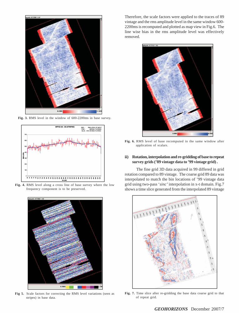
To compare the overall amplitude distribution in bothvintages, rms amplitude level over 600-2200ms window iscomputed for each trace and colour coded rms amplitudemaps were prepared. It was found that in general the rmsamplitude level in 89 vintage is about 160 times less than thatof 99 vintage. In addition, the rms amplitude map of 89 vintageshown in Fig.3 brought out the line to line rms amplitudevariation seen as stripes. Fig.4 shows a plot of rms amplitudevs in-line number along a cross line. The high frequencyvariation in rms amplitude level is smoothened by a medianfilter followed by local averaging. The ratio between thesmoothed curve and the original curve is saved as the scalefactor to be applied for bringing the rms amplitude level tothe background smooth level. The scalars computed for theentire survey are shown in map view in Fig.5. The scalefactors show the alignment of the stripes and no other pattern.

Fig 2a. A NS geological cross section shows the distribution of Karstified layers and dominance of intensely karstified layers. Yellow shows intenslykarstfied zone, green fractured and blue chalky karst zones.

Fig 2b. An EW geological cross section shows the distribution of Karstified layers and dominance of intenselykarstified layers. Yellow showsintensly karstfied zone, green fractured and blue chalky karst zones.

Table 1: Acquisition Parameters of the two Vintages

Acquisition Vintage 89 Vintage 99Parameter

No. of streamers 2 4Streamer separation 175m 150mNo. of channels per 96 160mstreamerGroup Interval 25m 12.5mSources Single Air gun array Dual Air gun arrays

(flip/flop shooting)Shot Interval 25m 12.5mNear offset 165m 140mFar offset 2513m 2140mFoldage 48 80In line Bin 12.5m 12.5mX line Bin 87.5m 37.5m

GEOHORIZONS December 2007/7

Therefore, the scale factors were applied to the traces of 89vintage and the rms amplitude level in the same window 600-2200ms is recomputed and plotted as map view in Fig.6. Theline wise bias in the rms amplitude level was effectivelyremoved.

Fig. 3. RMS level in the window of 600-2200ms in base survey.

Fig. 4. RMS level along a cross line of base survey where the lowfrequency component is to be preserved.

Fig 5. Scale factors for correcting the RMS level variations (seen asstripes) in base data.

Fig. 6. RMS level of base recomputed in the same window afterapplication of scalars.

ii) Rotation, interpolation and re-gridding of base to repeatsurvey grids (’89 vintage data to ’99 vintage grid) .

The fine grid 3D data acquired in 99 differed in gridrotation compared to 89 vintage. The coarse grid 89 data wasinterpolated to match the bin locations of ’99 vintage datagrid using two-pass ‘sinc’ interpolation in x-t domain. Fig.7shows a time slice generated from the interpolated 89 vintage

Fig. 7. Time slice after re-gridding the base data coarse grid to thatof repeat grid.

GEOHORIZONS December 2007/8

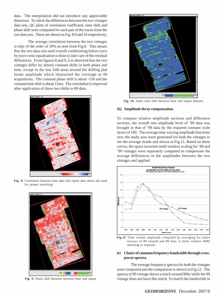
data. The interpolation did not introduce any appreciabledistortion. To check the differences between the two vintagesdata sets, QC plots of correlation coefficient, time shift andphase shift were computed for each pair of the traces from thetwo data sets. These are shown in Fig. 8,9 and 10 respectively.

The average correlation between the two vintagesis only of the order of 50% as seen from Fig.8. This meansthat the two data sets need overall conditioning before traceby trace cross equalisation is done to take care of the residualdifferences. From figures 8 and 9, it is observed that the twovintages differ by almost constant shifts in both phase andtime, except in the low fold areas around the drilling platforms amplitude which obstructed the coverage in 99acquisitions. The constant phase shift is about -150 and theconstant time shift is about 12ms. The correlation is improvedafter application of these two shifts to 89 data.

iii) Amplitude decay compensation.

To compare relative amplitude sections and differencesections, the overall rms amplitude level of ’89 data wasbrought to that of ’99 data by the required constant scalefactor of 160. The average time varying amplitude functionsover the study area were generated for both the vintages tosee the average trends and shown in Fig.11. Based on thesecurves, the space invariant multi window scaling for ’89 and’99 vintages were separately computed to compensate theaverage differences in the amplitudes between the twovintages and applied.

Fig. 8. Correlation between base data and repeat data shows the needfor proper matching.

Fig. 9. Phase shift between between base and repeat

Fig. 10. Static time shift between base and repeat datasets

Fig.11. Time variant amplitude computed by averaging for entiresurveys of 89 rotated and 99 data. A multi window RMSmatching is required.

iv) Choice of common frequency bandwidth through cross-power spectra.

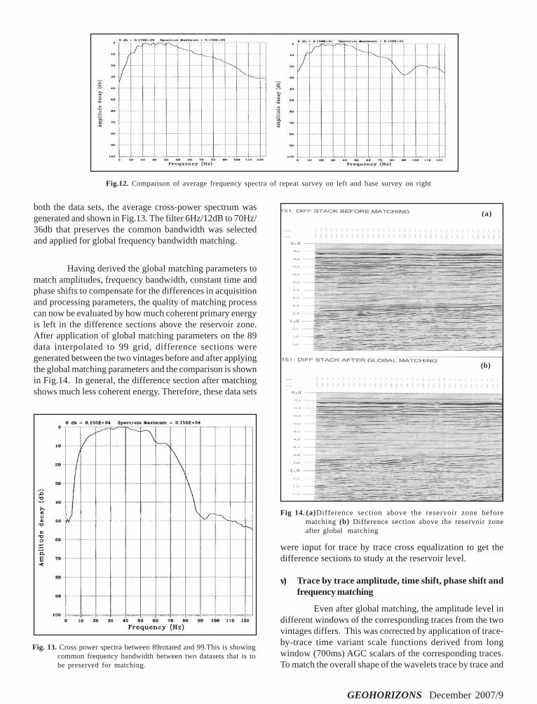
The average frequency spectra for both the vintageswere computed and the comparison is shown in Fig.12. Thespectra of 89 vintage shows a notch around 90hz while the 99vintage does not have this notch. To match the bandwidth in

GEOHORIZONS December 2007/9

were input for trace by trace cross equalization to get thedifference sections to study at the reservoir level.

v) Trace by trace amplitude, time shift, phase shift andfrequency matching

Even after global matching, the amplitude level indifferent windows of the corresponding traces from the twovintages differs. This was corrected by application of trace-by-trace time variant scale functions derived from longwindow (700ms) AGC scalars of the corresponding traces.To match the overall shape of the wavelets trace by trace and

Fig. 13. Cross power spectra between 89rotated and 99.This is showingcommon frequency bandwidth between two datasets that is tobe preserved for matching.

both the data sets, the average cross-power spectrum wasgenerated and shown in Fig.13. The filter 6Hz/12dB to 70Hz/36db that preserves the common bandwidth was selectedand applied for global frequency bandwidth matching.

Having derived the global matching parameters tomatch amplitudes, frequency bandwidth, constant time andphase shifts to compensate for the differences in acquisitionand processing parameters, the quality of matching processcan now be evaluated by how much coherent primary energyis left in the difference sections above the reservoir zone.After application of global matching parameters on the 89data interpolated to 99 grid, difference sections weregenerated between the two vintages before and after applyingthe global matching parameters and the comparison is shownin Fig.14. In general, the difference section after matchingshows much less coherent energy. Therefore, these data sets

Fig 14. (a)Difference section above the reservoir zone beforematching (b) Difference section above the reservoir zoneafter global matching

(a)

(b)

Fig.12. Comparison of average frequency spectra of repeat survey on left and base survey on right

GEOHORIZONS December 2007/10

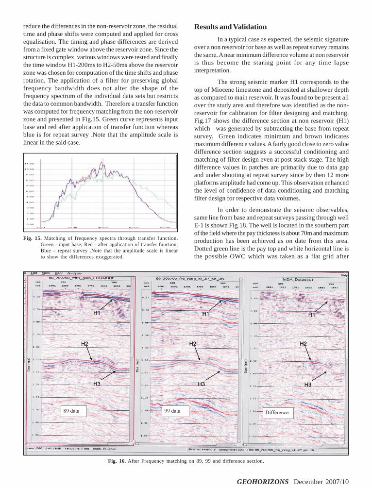
reduce the differences in the non-reservoir zone, the residualtime and phase shifts were computed and applied for crossequalisation. The timing and phase differences are derivedfrom a fixed gate window above the reservoir zone. Since thestructure is complex, various windows were tested and finallythe time window H1-200ms to H2-50ms above the reservoirzone was chosen for computation of the time shifts and phaserotation. The application of a filter for preserving globalfrequency bandwidth does not alter the shape of thefrequency spectrum of the individual data sets but restrictsthe data to common bandwidth. Therefore a transfer functionwas computed for frequency matching from the non-reservoirzone and presented in Fig.15. Green curve represents inputbase and red after application of transfer function whereasblue is for repeat survey .Note that the amplitude scale islinear in the said case.

Results and Validation

In a typical case as expected, the seismic signatureover a non reservoir for base as well as repeat survey remainsthe same. A near minimum difference volume at non reservoiris thus become the staring point for any time lapseinterpretation.

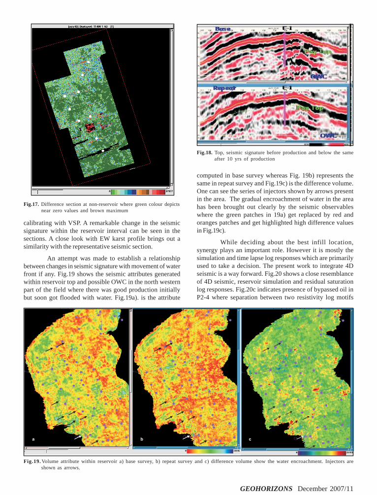
The strong seismic marker H1 corresponds to thetop of Miocene limestone and deposited at shallower depthas compared to main reservoir. It was found to be present allover the study area and therefore was identified as the non-reservoir for calibration for filter designing and matching.Fig.17 shows the difference section at non reservoir (H1)which was generated by subtracting the base from repeatsurvey. Green indicates minimum and brown indicatesmaximum difference values. A fairly good close to zero valuedifference section suggests a successful conditioning andmatching of filter design even at post stack stage. The highdifference values in patches are primarily due to data gapand under shooting at repeat survey since by then 12 moreplatforms amplitude had come up. This observation enhancedthe level of confidence of data conditioning and matchingfilter design for respective data volumes.

In order to demonstrate the seismic observables,same line from base and repeat surveys passing through wellE-1 is shown Fig.18. The well is located in the southern partof the field where the pay thickness is about 70m and maximumproduction has been achieved as on date from this area.Dotted green line is the pay top and white horizontal line isthe possible OWC which was taken as a flat grid after

Fig. 15. Matching of frequency spectra through transfer function.Green - input base; Red - after application of transfer function;Blue – repeat survey .Note that the amplitude scale is linearto show the differences exaggerated.

Fig. 16. After Frequency matching on 89, 99 and difference section.

GEOHORIZONS December 2007/11

calibrating with VSP. A remarkable change in the seismicsignature within the reservoir interval can be seen in thesections. A close look with EW karst profile brings out asimilarity with the representative seismic section.

An attempt was made to establish a relationshipbetween changes in seismic signature with movement of waterfront if any. Fig.19 shows the seismic attributes generatedwithin reservoir top and possible OWC in the north westernpart of the field where there was good production initiallybut soon got flooded with water. Fig.19a). is the attribute

Fig.18. Top, seismic signature before production and below the sameafter 10 yrs of production

Fig.17. Difference section at non-reservoir where green colour depictsnear zero values and brown maximum

computed in base survey whereas Fig. 19b) represents thesame in repeat survey and Fig.19c) is the difference volume.One can see the series of injectors shown by arrows presentin the area. The gradual encroachment of water in the areahas been brought out clearly by the seismic observableswhere the green patches in 19a) get replaced by red andoranges patches and get highlighted high difference valuesin Fig.19c).

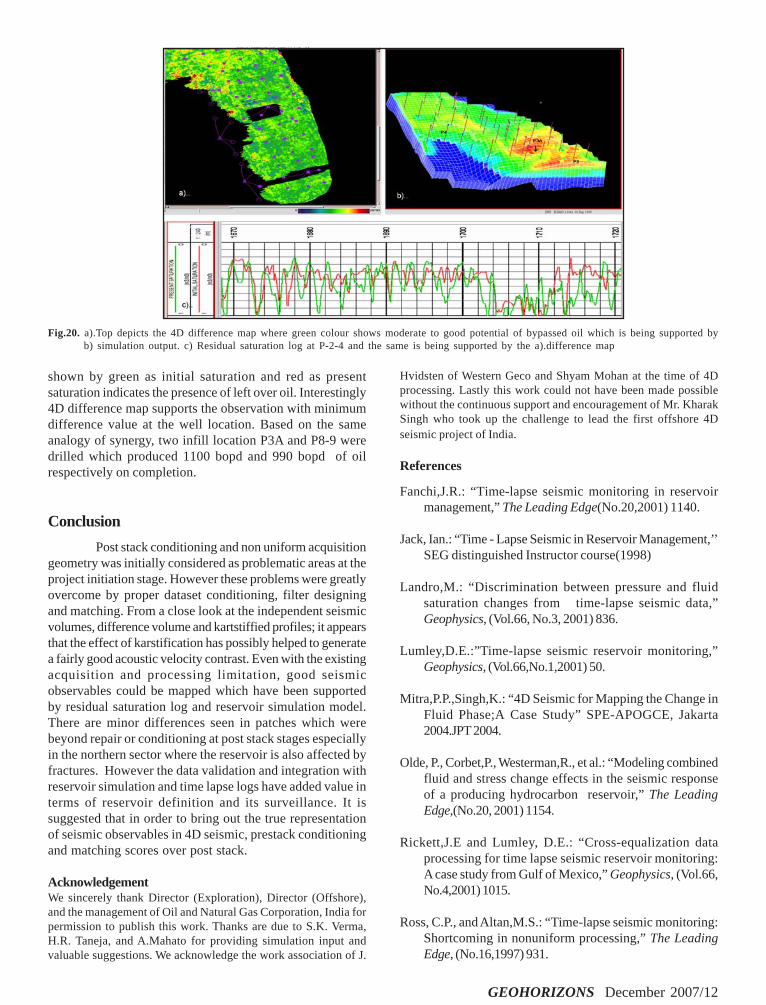
While deciding about the best infill location,synergy plays an important role. However it is mostly thesimulation and time lapse log responses which are primarilyused to take a decision. The present work to integrate 4Dseismic is a way forward. Fig.20 shows a close resemblanceof 4D seismic, reservoir simulation and residual saturationlog responses. Fig.20c indicates presence of bypassed oil inP2-4 where separation between two resistivity log motifs

Fig.19. Volume attribute within reservoir a) base survey, b) repeat survey and c) difference volume show the water encroachment. Injectors areshown as arrows.

GEOHORIZONS December 2007/12

shown by green as initial saturation and red as presentsaturation indicates the presence of left over oil. Interestingly4D difference map supports the observation with minimumdifference value at the well location. Based on the sameanalogy of synergy, two infill location P3A and P8-9 weredrilled which produced 1100 bopd and 990 bopd of oilrespectively on completion.

Conclusion

Post stack conditioning and non uniform acquisitiongeometry was initially considered as problematic areas at theproject initiation stage. However these problems were greatlyovercome by proper dataset conditioning, filter designingand matching. From a close look at the independent seismicvolumes, difference volume and kartstiffied profiles; it appearsthat the effect of karstification has possibly helped to generatea fairly good acoustic velocity contrast. Even with the existingacquisition and processing limitation, good seismicobservables could be mapped which have been supportedby residual saturation log and reservoir simulation model.There are minor differences seen in patches which werebeyond repair or conditioning at post stack stages especiallyin the northern sector where the reservoir is also affected byfractures. However the data validation and integration withreservoir simulation and time lapse logs have added value interms of reservoir definition and its surveillance. It issuggested that in order to bring out the true representationof seismic observables in 4D seismic, prestack conditioningand matching scores over post stack.

AcknowledgementWe sincerely thank Director (Exploration), Director (Offshore),and the management of Oil and Natural Gas Corporation, India forpermission to publish this work. Thanks are due to S.K. Verma,H.R. Taneja, and A.Mahato for providing simulation input andvaluable suggestions. We acknowledge the work association of J.

Hvidsten of Western Geco and Shyam Mohan at the time of 4Dprocessing. Lastly this work could not have been made possiblewithout the continuous support and encouragement of Mr. KharakSingh who took up the challenge to lead the first offshore 4Dseismic project of India.

References

Fanchi,J.R.: “Time-lapse seismic monitoring in reservoirmanagement,” The Leading Edge(No.20,2001) 1140.

Jack, Ian.: “Time - Lapse Seismic in Reservoir Management,’’SEG distinguished Instructor course(1998)

Landro,M.: “Discrimination between pressure and fluidsaturation changes from time-lapse seismic data,”Geophysics, (Vol.66, No.3, 2001) 836.

Lumley,D.E.:”Time-lapse seismic reservoir monitoring,”Geophysics, (Vol.66,No.1,2001) 50.

Mitra,P.P.,Singh,K.: “4D Seismic for Mapping the Change inFluid Phase;A Case Study” SPE-APOGCE, Jakarta2004.JPT 2004.

Olde, P., Corbet,P., Westerman,R., et al.: “Modeling combinedfluid and stress change effects in the seismic responseof a producing hydrocarbon reservoir,” The LeadingEdge,(No.20, 2001) 1154.

Rickett,J.E and Lumley, D.E.: “Cross-equalization dataprocessing for time lapse seismic reservoir monitoring:A case study from Gulf of Mexico,” Geophysics, (Vol.66,No.4,2001) 1015.

Ross, C.P., and Altan,M.S.: “Time-lapse seismic monitoring:Shortcoming in nonuniform processing,” The LeadingEdge, (No.16,1997) 931.

Fig.20. a).Top depicts the 4D difference map where green colour shows moderate to good potential of bypassed oil which is being supported byb) simulation output. c) Residual saturation log at P-2-4 and the same is being supported by the a).difference map