1

Post-Estimation Techniques in Statistical Analysis:

Introduction to Clarify and S-Post in Stata

PRISM BrownbagNovember 16, 2004

By: Kevin Sweeney and Brandon Bartels Presenters: Dave Darmofal and Corwin Smidt

(Note: If you’re not in Political Science come talk to me to log in.)

Preliminaries

• We will be posting these Powerpoint presentations to the PRISM “Luncheons” webpage:

http://psweb.sbs.ohio-state.edu/prism/luncheons.htm

• Also, you will be logging—via a .log file—all of the S-Post and Clarify procedures you are about to run.

• Bottom line: Everything said and done here will be on the record, so there’s less of a need to take extensive notes.

• Commands we’ll be using in S-Post:– Open Notepad. StartàProgramsàAccessoriesàNotepad– I: àgeneralàSpost&ClarifyàPost-estimation commands.txt

2

Introduction

• Three S’s of statistical analysis:– Sign– Significance– Strength, or substantive importance

• The effect of an independent variable on the dependent variable is “a change in an outcome for a change in an independent variable, holding all other variables constant” (Long 1997, 6).

• Most quantitative articles in leading journals contain post-estimation calculations of substantive effects of the independent variables of interest.

Effects in Linear and Non-Linear Models• Examining marginal effects in OLS is easy: β . A one-unit

change in X produces a β -unit change in Y, holding other variables constant.

• Examining effects in nonlinear models, such as logit, probit, ordered probit, and other ML models, is less straightforward. Marginal effects with respect to X are not constant (note: but not interactive).

• In nonlinear models, the magnitude of the change in the probability of an event occurring, given a change in a particular independent variable, depends on the levels of the other independent variables.

• S-Post (Long) and Clarify (Tomz, Wittenberg, and King) make post-estimation easy and offer a powerful means of presenting the substantive results from a statistical analysis.

3

What S-Post Can Do

• For a comprehensive presentation of S-Post, see:– Long, J. Scott, and Jeremy Freese. 2001. Regression Models for

Categorical Dependent Variables Using Stata. College Station, TX: Stata Press.

– Once S-Post is installed, the “help” files provide very good information on the commands. E.g, “help prchange”.

• For those who don’t usually use Stata, J. Scott Long and Simon Cheng also have Excel spreadsheets available to download which are easy to use and present nice graphs. Download at: http://www.indiana.edu/~jslsoc/xpost.htm

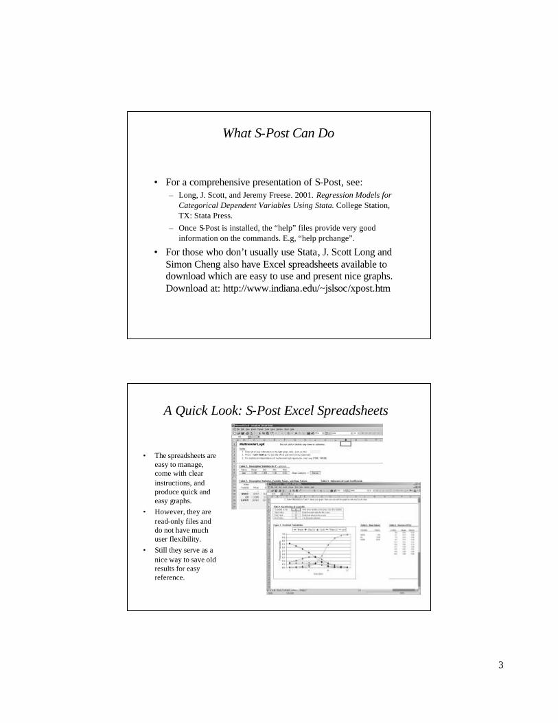
A Quick Look: S-Post Excel Spreadsheets

• The spreadsheets are easy to manage, come with clear instructions, and produce quick and easy graphs.

• However, they are read-only files and do not have much user flexibility.

• Still they serve as a nice way to save old results for easy reference.

4

What S-Post Can Do – Key Commands

• fitstat – goodness-of-fit measures• listcoef – odds ratios• prvalue & prtab – predicted probabilities for

particular covariate profiles.• prchange – first differences• prgen – setup for graphing• Again, use the “help” files in Stata if you get stuck on

these.• These commands can be used in:

– regress, logit, probit, ologit, oprobit, mlogit, clogit, cloglog, poisson, nbreg,cnreg, intreg, tobit, zip, zinb

Open a Log File

5

Open a Log File

Use pull-down menu and change from “Formatted Log” to “Log” – makes it easy to open in Word or Textpad. Save to K-drive.

Installing S-PostStep 1

net from http://www.indiana.edu/~jslsoc/stata/

6

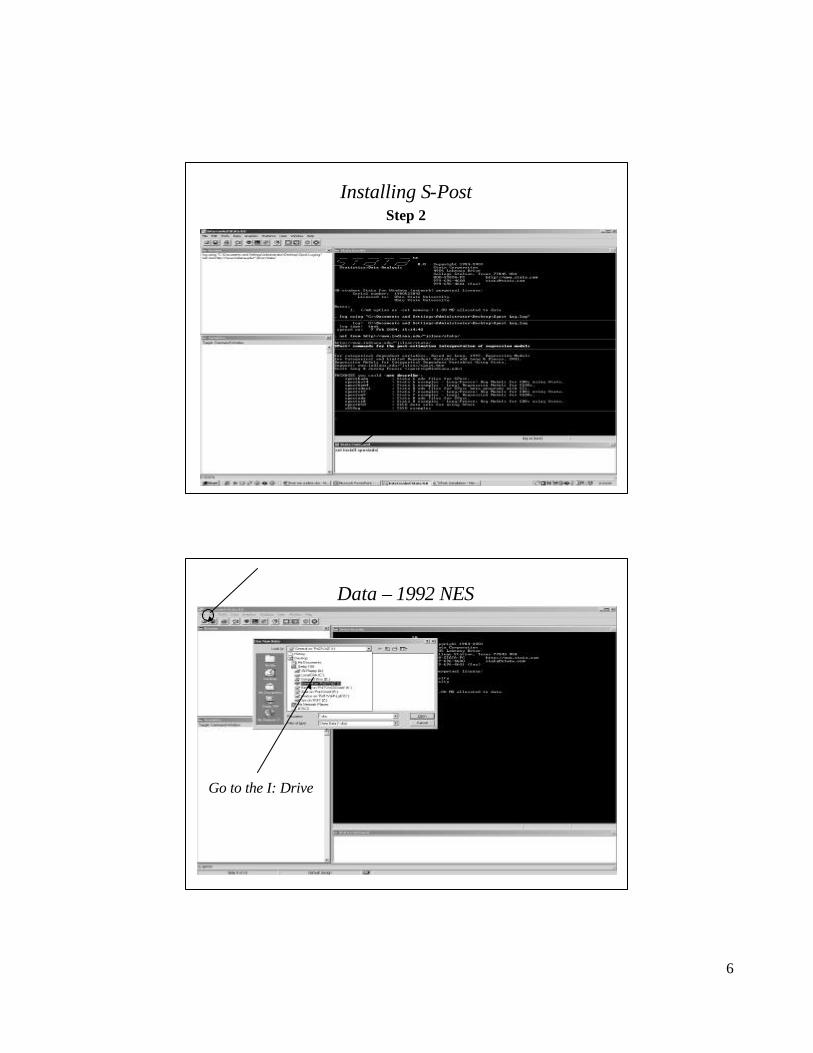
Installing S-PostStep 2

net install spostado

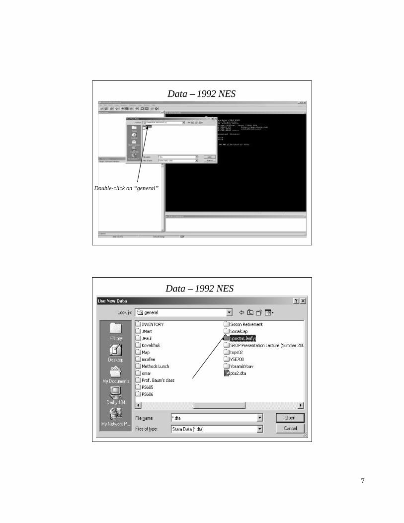
Data – 1992 NES

Go to the I: Drive

7

Data – 1992 NES

Double-click on “general”

Data – 1992 NES

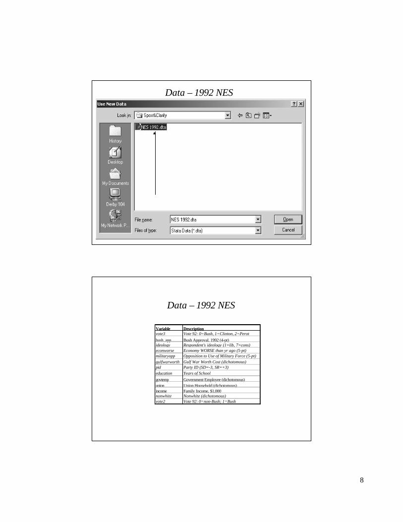
Double-click on “NES 1992.dta”

8

Data – 1992 NES

Data – 1992 NES

Variable Descriptionvote3 Vote 92: 0=Bush, 1=Clinton, 2=Perotbush_app Bush Approval, 1992 (4-pt)ideology Respondent's ideology (1=lib, 7=cons)econworse Economy WORSE than yr ago (5-pt)militaryopp Opposition to Use of Military Force (5-pt)gulfwarworth Gulf War Worth Cost (dichotomous)pid Party ID (SD=-3, SR=+3)education Years of Schoolgovtemp Government Employee (dichotomous)union Union Household (dichotomous)income Family Income, $1,000nonwhite Nonwhite (dichotomous)vote2 Vote 92: 0=non-Bush; 1=Bush

9

Goodness-of-Fit Measuresfitstat

• Logit and Probit report one pseudo-R2 measure: McFadden’s R2: (init LL – final LL)/(init LL).

• There are other pseudo-R2 measures, too; see Long (1997, 104-113). • Two statistics that are often reported in journal articles: percent

correctly predicted (PCP; using a 0.5 threshold) and proportional reduction in error (PRE) – although see Train 2003, p.73 for why their theoretical basis is questionable.

• PRE is a measure comparing the predictive success of the estimated model to a null model, i.e., proportion of the DV in the modal category (PMC).

• PRE = (PCP – PMC)/(1 – PMC)• The fitstat command can give these to you in an instant! Also

available for models other than logit and probit.• Let’s estimate a simple vote choice model to check it out.• logit vote2 pid econworse militaryopp education nonwhite

Goodness-of-Fit Measures

10

Goodness-of-Fit Measures

Simply type “fitstat” in the command window

“Count R2” is PCP “Adj Count R2” is PRE

Goodness-of-Fit Measures

PRE

11

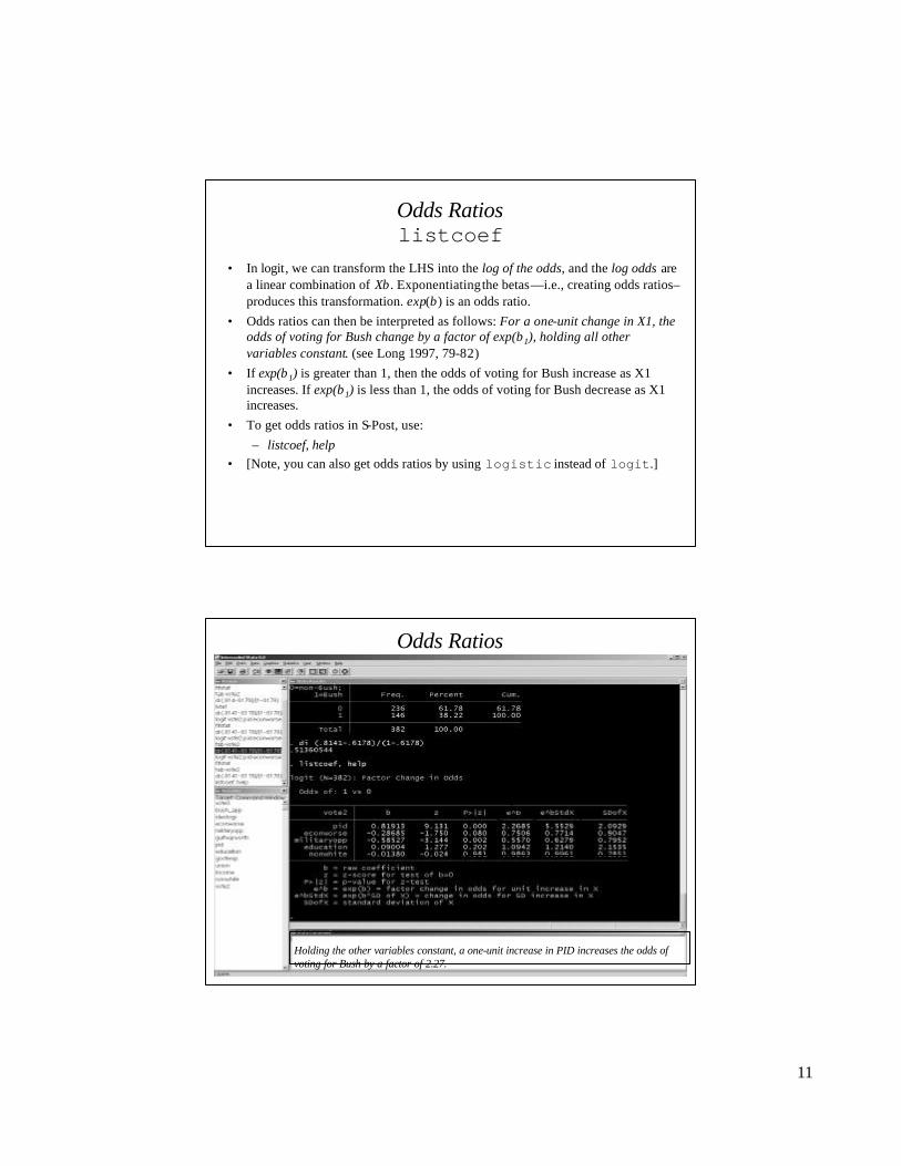
• In logit, we can transform the LHS into the log of the odds, and the log odds are a linear combination of Xβ. Exponentiatingthe betas—i.e., creating odds ratios–produces this transformation. exp(β) is an odds ratio.

• Odds ratios can then be interpreted as follows: For a one-unit change in X1, the odds of voting for Bush change by a factor of exp(β1), holding all other variables constant. (see Long 1997, 79-82)

• If exp(β1) is greater than 1, then the odds of voting for Bush increase as X1 increases. If exp(β1) is less than 1, the odds of voting for Bush decrease as X1 increases.

• To get odds ratios in S-Post, use:– listcoef, help

• [Note, you can also get odds ratios by using logistic instead of logit.]

Odds Ratioslistcoef

Odds Ratios

Odds Ratios for a 1-unit change in X

Odds Ratios for a 1-SD change in X

Holding the other variables constant, a one-unit increase in PID increases the odds of voting for Bush by a factor of 2.27.

12

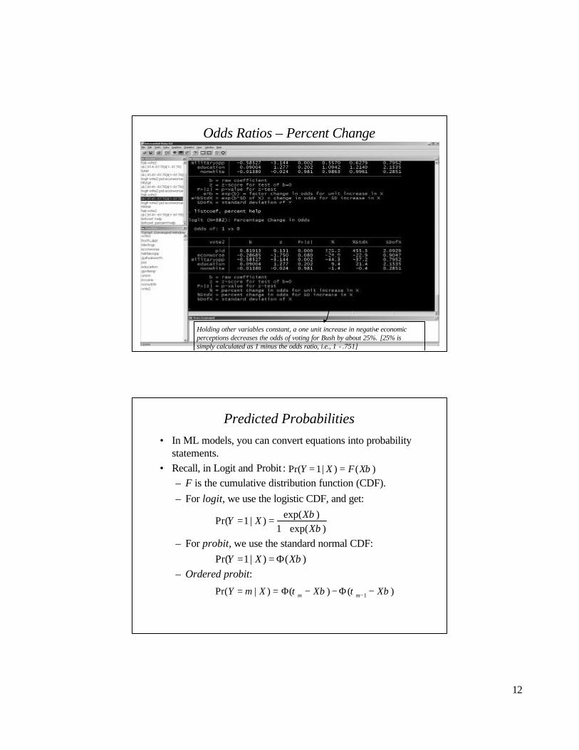
Odds Ratios – Percent Change

Holding other variables constant, a one unit increase in negative economic perceptions decreases the odds of voting for Bush by about 25%. [25% is simply calculated as 1 minus the odds ratio, i.e., 1 - .751]

Percent change in the odds instead of factor change.

Predicted Probabilities• In ML models, you can convert equations into probability

statements. • Recall, in Logit and Probit :

– F is the cumulative distribution function (CDF). – For logit, we use the logistic CDF, and get:

– For probit, we use the standard normal CDF:

– Ordered probit:

)()|1Pr( βXFXY ==

)exp(1)exp(

)|1Pr(β

βX

XXY

+==

)()|1Pr( βXXY Φ==

)()()|Pr( 1 βτβτ XXXmY mm −Φ−−Φ== −

13

Predicted Probabilities• In our logit model of vote choice:

• Present results in terms of probability to draw conclusions about the substantive importance of variables.

• A number of ways to do this:– Predicted probabilities for various covariate profiles . – First differences . Change in the probability of an event occurring

given a particular change in an IV, holding other variables constant at baseline values.

– Graphing the probability of an event occurring as a function of an IV of interest, holding other variables constant at baseline values.

)exp(1)exp(

)|1Pr(543210

543210

NonwhiteEducMilitEconPIDNonwhiteEducMilitEconPID

XYββββββ

ββββββ++++++

+++++==

Predicted Probabilities for Covariate Profilesprvalue

• Let’s say I wanted to know the probability that a highly educated individual who is strongly opposed to military force voted for Bush.

• Use prvalue to set these two particular variables to the desired values, and set the other variables to baseline values (I will set everything to mean levels).

• Basic syntax: prvalue, x(education max militaryopp max) rest(mean)

14

Predicted Probabilities for Covariate Profiles

Probability of a highly educated individual who is strongly opposed to military force (holding the other variables constant at their means) voting for Bush is about 0.14.

Cross-Tabs of Predicted Probabilitiesprtab

• Another way to present probabilities for particular covariate profiles is by creating a cross-tab of probabilities.

• S-Post’s prtab command computes a table of predicted probabilities for all combinations of as many as 4 categorical variables.

• Let’s say I wanted to examine the probability of voting Bush given all possible covariate profiles of PID and negative economic perceptions, holding other variables constant at their mean values.

• Syntax: prtab pid econworse, rest(mean)

15

Cross-Tabs of Predicted Probabilities

35 covariate profiles

First Differencesprchange

• First difference: The change in the probability of voting for Bush given a particular change in an independent variable, holding all other variables constant at some baseline value (e.g., means or modes for dichotomous variables). I recommend using Clarify to do these, but I’ll quickly run through the syntax.

• prchange calculates these for you.• First, do a set mat command to expand the matrix in Stata.

set mat 60prchange, help

16

First Differencesprchange

First Differencesprchange, fromto

prchange, fromto help

17

Graphsprgen

• Graphing is a very powerful way to present the results of a statistical model.

• Let’s say we wanted to graph the probability of an event occurring as a function of an independent variable of interest.

• To show you that I can use S-Post outside of logit, let’s run a multinomial logit model of vote choice, with Bush, Clinton, and Perot as the three nominal outcomes of the DV.

mlogit vote3 pid econworse militaryopp education nonwhite, basecategory(0)

• [Note: One can test whether this model violates the I.I.A. assumption using S-Post’s mlogtest command. Do “help mlogtest” for more info.]

Graphsprgen

18

Graphsprgen

• Effect of economic perceptions on vote choice? Graph the probabilities of voting for Bush, Clinton, and Perot as a function of economic perceptions, holding other variables constant at a baseline value.

prgen econworse, gen(econ)• Note: the default settings generate predicted probabilities of voting

for each of the three candidates as “econworse” ranges from its minimum (1) to maximum (5) value (holding other variables at their mean levels).

• See “help prgen” for more options.

Graphsprgen

7 new variables

19

Graphsprgen

• To produce a simple graph of the effect of economic perceptions,use the line function:

line econp0 econp1 econp2 econx, ytitle(Probability) xtitle(Negative Economic Perceptions)

• One always lists the y-axis variables upfront with the x-axis variable (econx) coming last.

Graphsprgen

20

Graphing Hints in Stata

• The problem with the line command is that it is only useful if you have a color printer since it doesn’t allow line symbols for differentiation.

• While some individuals resort to using Excel for graphs, it would be well worth your time to learn the graphing capabilities of Stata, especially scatter in this case.

• scatter is Stata’s scatterplot graph command which allows for symbols to mark the lines. One only needs to make a few simple adjustments to it for one to produce a clean and highly informative graph. Since Stata’s graphing help file is huge, I thought I would highlight a few, key commands to implement.

Scatter Commands• First, graph adjustment commands are all made after the comma:

scatter var1 var2 varx, adjustment commands…..• One should first use msymbol() to assign symbols to each y-variable

and then connect the symbols with lines using connect():scatter var1 var2 varx, msymbol(d x) connect(l l)

where msymbol options include:d – diamond, x – x-mark, s – square, + --plus, o – circle, . -dot, Dh – large hollow diamond,

Sh – large hollow square, Oh – large hollow circle, and many more…

and l within connect connects each variable by a line. • Note: the symbol and connect commands apply in order to each y-

variable, where one uses a space to distinguish between variables. • To title each axis use the xtitle(…) and ytitle(…) commands, with the

titles typed within the parentheses. Use the label var command to label the variables so the legend is more descriptive.

21

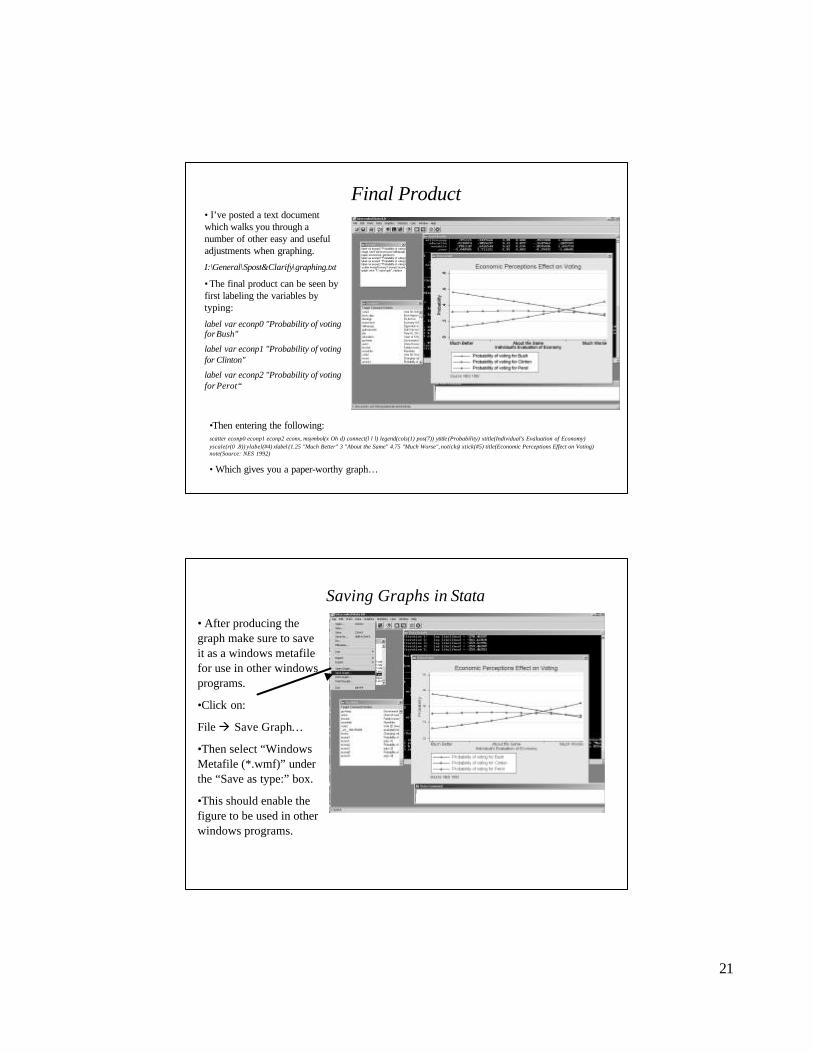
Final Product• I’ve posted a text document which walks you through a number of other easy and useful adjustments when graphing.

I:\General\Spost&Clarify\graphing.txt

• The final product can be seen by first labeling the variables by typing:

label var econp0 "Probability of voting for Bush"

label var econp1 "Probability of voting for Clinton"

label var econp2 "Probability of voting for Perot“

•Then entering the following:scatter econp0 econp1 econp2 econx, msymbol(x Oh d) connect(l l l) legend(cols(1) pos(7)) ytitle (Probability) xtitle(Individual's Evaluation of Economy)yscale(r(0 .8)) ylabel(#4) xlabel (1.25 "Much Better" 3 "About the Same" 4.75 "Much Worse", noticks) xtick(#5) title(Economic Perceptions Effect on Voting) note(Source: NES 1992)

• Which gives you a paper-worthy graph…

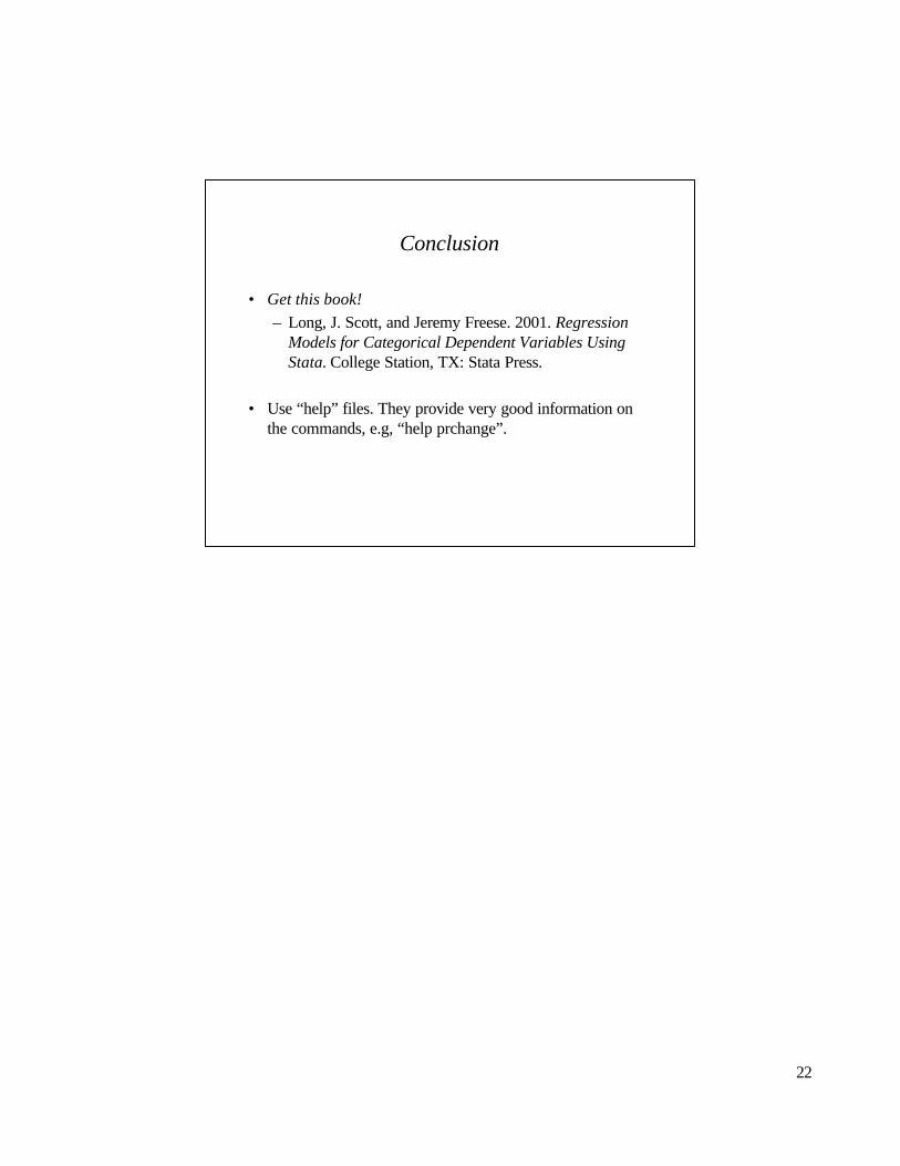
Saving Graphs in Stata

• After producing the graph make sure to save it as a windows metafile for use in other windows programs.

•Click on:

File à Save Graph…

•Then select “Windows Metafile (*.wmf)” under the “Save as type:” box.

•This should enable the figure to be used in other windows programs.

22

Conclusion

• Get this book!– Long, J. Scott, and Jeremy Freese. 2001. Regression

Models for Categorical Dependent Variables Using Stata. College Station, TX: Stata Press.

• Use “help” files. They provide very good information on the commands, e.g, “help prchange”.