ARTICLE IN PRESS

0378-4371/$ - se

doi:10.1016/j.ph

�CorrespondE-mail addr

1Conditional

models are desi

Physica A 375 (2007) 612–624

www.elsevier.com/locate/physa

Portfolio management under sudden changes in volatility andheterogeneous investment horizons

Viviana Fernandeza,�, Brian M. Luceyb

aCenter for Applied Economics (CEA), Department of Industrial Engineering of the University of Chile, Santiago, ChilebInstitute for International Integration Studies, Trinity College Dublin, Ireland

Received 6 April 2006; received in revised form 26 September 2006

Available online 27 October 2006

Abstract

We analyze the implications for portfolio management of accounting for conditional heteroskedasticity and sudden

changes in volatility, based on a sample of weekly data of the Dow Jones Country Titans, the CBT-municipal bond, spot

and futures prices of commodities for the period 1992–2005. To that end, we first proceed to utilize the ICSS algorithm to

detect long-term volatility shifts, and incorporate that information into PGARCH models fitted to the returns series. At

the next stage, we simulate returns series and compute a wavelet-based value at risk, which takes into consideration the

investor’s time horizon. We repeat the same procedure for artificial data generated from semi-parametric estimates of the

distribution functions of returns, which account for fat tails. Our estimation results show that neglecting GARCH effects

and volatility shifts may lead to an overestimation of financial risk at different time horizons. In addition, we conclude that

investors benefit from holding commodities as their low or even negative correlation with stock and bond indices

contribute to portfolio diversification.

r 2006 Elsevier B.V. All rights reserved.

Keywords: Structural volatility shifts; Heterogeneous investors; Wavelets; Value at risk

1. Introduction

To date, there is an extensive literature on the behavior of volatility of assets returns and the effect of this onboth the value and composition of investors portfolios. Indeed, the GARCH model and its numerousextensions have been widely used to account for the existence of conditional heteroskedasticity in financialtime series (see, for instance, the survey by Poon and Granger [1]).1 However, less attention has been paid tothe detection of multiple shifts in unconditional variance over time. For example Ref. [2] et seq. conclude thatpersistence in variance may be overstated by not accounting for deterministic structural breakpoints in thevariance model.

e front matter r 2006 Elsevier B.V. All rights reserved.

ysa.2006.10.004

ing author. Tel.: +56 2 978 4072; fax: +56 2 689 7895.

esses: vfernand@dii.uchile.cl (V. Fernandez), blucey@tcd.ie (B.M. Lucey).

heteroskedasticity means that the variance of a return series changes over time, conditional on past information. GARCH

gned to capture the time-series dynamics of returns, in which we observe persistence or serial correlation in volatility.

ARTICLE IN PRESSV. Fernandez, B.M. Lucey / Physica A 375 (2007) 612–624 613

A relatively recent approach to testing for volatility shifts is the Iterative Cumulative Sums of Squares(ICSS) approach of Ref. [3]. This algorithm allows for detecting multiple breakpoints in variance in a timeseries. Examples of this approach to equity markets include [4–6]. Another subject, which has receivedattention in recent research and that also has important implications for portfolio management, is theexistence of heterogeneous investors. Ref. [7] points out that, for the specific case of commodity markets, long-horizon traders will essentially focus on price fundamentals that drive overall trends, whereas short-termtraders react to incoming information within a short-term horizon. Hence, market dynamics in the aggregatewill be the result of the interaction of agents with heterogeneous time horizons. In order to model the behaviorof financial series at different time spans, researchers have resorted to wavelet analysis. Wavelet analysis is arefinement of Fourier analysis that allows for decomposing a time series into its high frequency or noisycomponents and its low frequency or trend components, among many other applications. See Refs. [7–9] forcommodity and derivative markets, for interest and foreign exchange rates see Refs. [10,11], and for equitymarkets see Refs. [12–18]. Finally, one of the main issues in the analysis of portfolios is that of what thelikelihood is of a loss of a particular magnitude. This Value at Risk (VaR) analysis has attracted verysignificant attention in the economics and finance literature (see for example Refs. [19–21]) but relatively littlein econophysics (see Refs. [22–24] as exceptions). In essence the VaR approach provides an integratedapproach to examine and assess the probability of a given percentage loss of wealth over a given time period.

The aim of this article is two-fold. First, we analyze whether accounting for conditional heteroskedasticityand long-term volatility shifts in asset returns really matters when comes to quantifying the potential marketrisk an investor faces. In doing so, we consider different time horizons by resorting to a wavelet-baseddecomposition of VaR. Second, we look at the potential diversification gains in terms of the VaR decreaseobtained by adding commodities to a portfolio.

This article is organized as follows. Section 2 presents the main methodological tools utilized in theempirical section of the article. Section 3 presents some descriptive statistics of the data used in the simulationscarried out later on. Section 4 presents the simulation exercises involving a portfolio primarily composed ofstock indices and a portfolio that also include spot and futures positions in commodities. We discuss theimplications of not accounting for correlated volatility and volatility shifts for risk quantification. In addition,we focus on the benefits of holding commodities for portfolio diversification. Section 5 concludes.

2. Methodology

2.1. The ICSS algorithm

The derivation of the ICSS algorithm is based on the assumption that a time series has a stationaryunconditional variance over an initial time period until a sudden break takes place. The unconditionalvariance is then stationary until the next sudden change occurs. This process repeats through time, giving atime series of observations with M breakpoints in the unconditional variance along the sample:

s2t ¼

t20; 1otoi1;

t21; i1otoi2;

::::

t2M ; iMoton:

8>>>><>>>>:

(1)

In order to estimate the number of variance shifts and the point in time at which they occur, a cumulativesum of squares is computed, Ck ¼

Pkt¼1z

2t , k ¼ 1, 2,y,n, where {zt} is a series of uncorrelated random

variables with zero mean and unconditional variance s2t , as in (1). Define the statistic

� k ¼Ck

Cn

�k

n; k ¼ 1; 2; . . . ; n; � 0 ¼ � n ¼ 0 (2)

as the centered and normalized sum of squares.If no variance shifts are observed under the time period under consideration, � k will oscillate around zero.

Otherwise, if there is one or more sudden changes in variance, � k will breach given boundaries with high

ARTICLE IN PRESSV. Fernandez, B.M. Lucey / Physica A 375 (2007) 612–624614

probability. These boundaries are obtained from the asymptotic distribution of � k under the null hypothesisof constant variance.2 The ICSS algorithm systematically looks for breakpoints along the time period ofinterest. A full description of the algorithm is given in Ref. [3].

2.2. Wavelet-based betas

Wavelet-variance analysis consists of partitioning the variance of a time series into components that areassociated to different time scales. That is, this methodology enables us to conclude what scales are importantcontributors to the overall variability of a series (see Ref. [25]).

Let x1;x2; . . . ;xn be a time series of interest, assumed to be a realization of a stationary process withvariance s2X . If u

2X ðtjÞ denotes the wavelet variance for scale tj�2

j�1, then the following relationship holds:

s2X ¼X1j¼1

u2xðtjÞ. (3)

where the square root of the wavelet variance is expressed in the same units as the original data.Let n0j ¼ n=2j

� �be the number of discrete-wavelet transform (DWT) coefficients at level j, where n is the

sample size, and let L0j � ðL� 2Þð1� 1=2jÞ� �

be the number of DWT boundary coefficients3 at level j

(provided that n0j4L0j), where L is the width of the wavelet filter. An unbiased estimator of the waveletvariance is defined as

~u2X ðtjÞ �1

ðn0j � L0jÞ2j

Xn0j�1t¼L0

j�1

d2j;t. (4)

Given that the DWT de-correlates the data, the non-boundary wavelet coefficients at a given level (dj) arezero-mean Gaussian white-noise processes.

Similarly, the unbiased wavelet covariance between time series X and Y, at scale j, can be defined as

~u2XY ðtjÞ �1

ðn0j � L0jÞ2j

Xn0j�1t¼L0

j

dðX Þj;t d

ðY Þj;t , (5)

provided that n0j4L0j.However, as pointed out in Ref. [25], the sample properties of the DWT variance and covariance estimators

are inferior to those of non-decimated discrete wavelet transforms, also known as stationary wavelettransforms. The non-decimated DWT is a non-orthogonal variant of the DWT, which is time-invariant. Thatis, unlike the classical DWT, the output is not affected by the date at which we start recording a time series. Inaddition, the number of coefficients at each scale equals the number of observations in the original time series.A non-decimated form of the DWT is known as the maximal overlap DWT (MODWT).4 The unbiasedMODWT estimator of the wavelet variance is given by

u2X ðtjÞ �1

Mj

Xn�1t¼Lj�1

~d2

j;t (6)

where ~d2

j;t is the MODWT-wavelet coefficient at level j and time t, Mj � n2Lj þ 1, Lj � ð2j � 1ÞðL� 1Þ þ 1 is

the width of the MODWT filter for level j, and n is the number of observations in the original time series.While there are n MODWT-wavelet coefficients at each level j, the first (Lj21)-boundary coefficients arediscarded. (Retaining such boundary coefficients leads to a biased estimate.)

2Under the null hypothesis,ffiffiffiffiffiffiffiffin=2

p� k behaves asymptotically like a Brownian bridge.

3The bxc and dxe terms represent the greatest integer px and the smallest integer Xx, respectively. Boundary coefficients are those that

are formed by combining together some values from the beginning and the end of the time series.4The scaling ð~lkÞ and wavelet ð ~hkÞ filter coefficients for the MODWT are rescaled versions of those of the DWT. Specifically, ~lk � lk=

ffiffiffi2p

and ~hk � hk=ffiffiffi2p

.

ARTICLE IN PRESSV. Fernandez, B.M. Lucey / Physica A 375 (2007) 612–624 615

Likewise, the unbiased MODWT estimator of the wavelet covariance can be obtained as

u2XY ðtjÞ �1

Mj

Xn�1t¼L0

j

~dðX Þ

j;t~dðY Þ

j;t . (7)

In the asset-pricing model of Ref. [26], the wavelet-beta estimator for asset i, at scale j, is defined as

biðtjÞ ¼u2RiRm

ðtjÞ

u2RmðtjÞ

, (8)

where u2RiRmðtjÞ is the wavelet covariance of asset i and the market portfolio at scale j, and u2Rm

ðtjÞ is the waveletvariance of the market portfolio at scale j.

An R2 for each scale can be computed as follows (see Ref. [18]):

R2i ðtjÞ ¼ biðtjÞ

2u2RmðtjÞ

u2RiðtjÞ

. (9)

2.3. Wavelet-based value at risk

As discussed in Ref. [18], the empirical representation of the capital asset pricing model (CAPM) is given by

Ri � Rf ¼ ai þ biðRm � Rf Þ þ �i; k ¼ 1; 2; . . . ; k, (10)

where Ri, Rf, Rm are, respectively, the returns on asset i, the risk-free asset and the market portfolio, and ei isan error term with zero mean and variance s2� .

From Eq. (10), the variance of the excess return on asset i and the covariance of the excess returns on assets i

and j are given, respectively, by

s2i ¼ b2i s2m þ s2� ; i ¼ 1; 2; . . . ; k,

sij ¼ bibjs2m; i; j ¼ 1; 2; . . . ; k; iaj,

where Eð�2i Þ ¼ s2�i and Eð�i�jÞ ¼ 0 8iaj.Consequently, the variance–covariance matrix of the k excess returns is given by

X ¼ bb0s2m þ E, (11)

where b ¼

b1b2

..

.

bk

0BBBBB@

1CCCCCAand E ¼

s2�1 0 � � � 0

0 s2�2 � � � 0

..

. ... . .

. ...

0 0 . . . s2�k

0BBBBBB@

1CCCCCCA.

The (12a) %-Value at Risk (VaR) of a portfolio of k assets is then

VaRðaÞ ¼ V 0lðaÞffiffiffiffiffiffiffiffiffiffiffiffiffiffiffiffiffiffiffiffiffiffiffiffiffiffiffiffiffiffiffiffix0ðbb0s2m þ EÞx

q, (12)

where x is a k� 1 vector of portfolio weights, V0 is the initial value of the portfolio, and lðaÞ � F�1ð1� aÞ,where F(.) is the cumulative distribution function of the standard normal.

For an equally weighted portfolio, such that oi ¼ 1=k8i, the VaR boils down to

VaRðaÞ ¼ V 0lðaÞ

ffiffiffiffiffiffiffiffiffiffiffiffiffiffiffiffiffiffiffiffiffiffiffiffiffiffiffiffiffiffiffiffiffiffiffiffiffiffiffiffiffiffiffiffiffiffiffiffiffiffiffiffiffiffiffiffis2m

Xk

i¼1

bi=k

!2

þ1

k2

Xk

i¼1

s2�i

vuut . (13)

As k becomes large, VaRðaÞ � V 0lðaÞ

ffiffiffiffiffiffiffiffiffiffiffiffiffiffiffiffiffiffiffiffiffiffiffiffiffiffiffiffiffiffiffiffiffis2m

Pki¼1bi=k

� �2r. That is, for a well-diversified portfolio, all that

matters is systematic risk.

ARTICLE IN PRESSV. Fernandez, B.M. Lucey / Physica A 375 (2007) 612–624616

The VaR at scale j can be obtained by evaluating Eq. (13) at the j-scale components of the variance of themarket portfolio return, the betas of the k stocks, and of the variances of the error terms that capture non-systematic risk:

VaRtjðaÞ ¼ V 0lðaÞ

ffiffiffiffiffiffiffiffiffiffiffiffiffiffiffiffiffiffiffiffiffiffiffiffiffiffiffiffiffiffiffiffiffiffiffiffiffiffiffiffiffiffiffiffiffiffiffiffiffiffiffiffiffiffiffiffiffiffiffiffiffiffiffiffiffiffiffiffiffiffiffiffiffiffiffiffis2mðtjÞ

Xk

i¼1

biðtjÞ=k

!2

þ1

k2

Xk

i¼1

s2�i ðtjÞ

vuut . (14)

The variance of the error term at scale j is computed as

s2� ðtjÞ ¼ s2i ðtjÞ � b2i ðtjÞs2mðtjÞ, (15)

whereas the variance of stock i at scale j, s2i ðtjÞ, the beta of stock i return at scale j, biðtjÞ, and the variance ofthe market portfolio at scale j, s2mðtjÞ, can be computed using Eqs. (6) and (8).

2.4. Long-memory processes

Ref. [7] discusses how to obtain the long-memory parameter of a time series from wavelet analysis.Specifically, a time series yt is said to be a long-memory process if its autocovariance sequence decays at a rateslower than that of an autoregressive moving average (ARMA) process. Mathematically, if ls ¼

covðyt; ytþsÞ; s ¼ �1; 0; 1 and there exist constants C and b, such that lims!1ðls=CsbÞ ¼ 1, then yt is longmemory process. Furthermore, lims!1ðls=CsbÞ ¼ 1 if and only if limf!0ðSðf Þ=K jf jaÞ ¼ 1, where aþ b ¼ �1,K is a constant, jf jo1=2, and S(f) is the spectral density function of the process.

The exponent a is called the spectral exponent, and it has been shown to equal �2d, where d represents thelong-memory parameter, as usually referred to in time series analysis. Ref. [7] points out that d can beestimated from a regression of the logarithm of the wavelet variance on the logarithm of the scale. If 0odo1,yt is a long memory process. In particular, if 0odo0:5, yt is stationary but shocks decay at a hyperbolic rate,while if 0:5pdo1, yt is non-stationary. On the other hand, if �0:5oyto0 is stationary and has short memory.

3. The data

Our sample consists of weekly returns on the Dow Jones Country Titans Stock Indices (for Australia,Canada, Germany, Hong Kong, Italy, Japan, The Netherlands, Spain, Sweden, Switzerland, and The UnitedKingdom), the Dow Jones Global 50 stock index,5 the Dow Jones Industrial Average Stock index, Moody’scommodities index6, the CBT-municipal bond and CBT-10 year US T-note rates, the London Metal Exchangespot prices of copper, nickel and zinc, and the CME futures prices of corn and wheat. All indices and prices areexpressed in US dollars and span the period from January 1992 to December 2005. The data sources areDatastream and Ecowin.

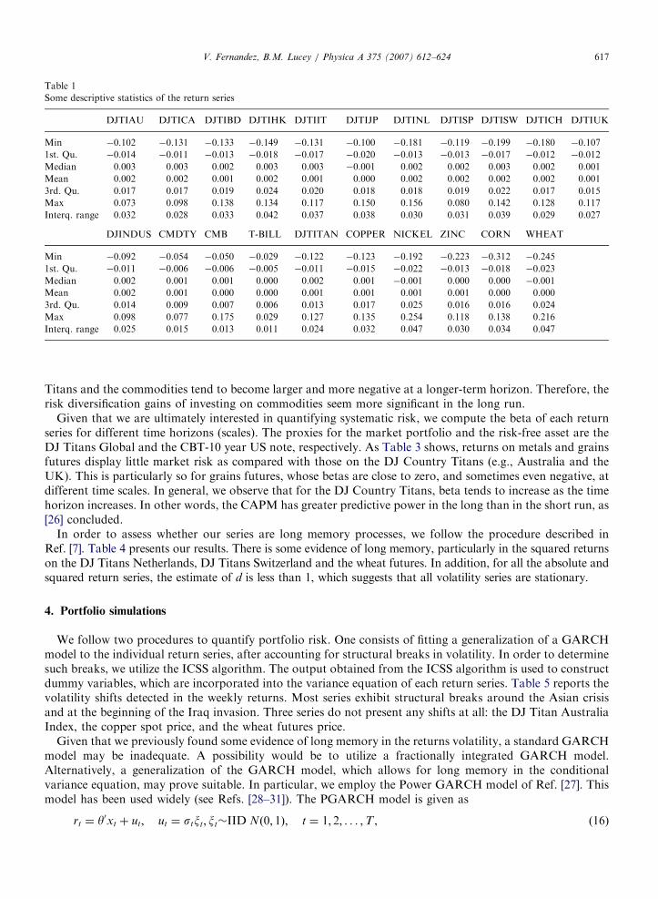
Table 1 presents some descriptive statistics of the data. The returns on the nickel spot price and the wheatfutures price stand out for their high volatility, measured by the interquartile range, followed by the DJ HongKong Titan. The least volatile return series are those on the Moody’s commodity index, the CBT-municipalbond and the CBT-10 year US note. As is usual for financial series, all return series strongly reject theassumption of normality, according to the Shapiro-Wilk and Jarque-Bera tests.

As pointed out earlier, recent research has shown the importance of the time scale when assessing financialrisk. As reported in Panels (a) and (b) of Table 2, the wavelet pair-wise correlation coefficients change overtime, suggesting that risk diversification depends on the investor’s time horizon. As we see, the correlationsbetween the DJ Titans tend to increase as we move to the upper scales, and the correlations between the DJ

5The Dow Jones Global Titans is made up of 50 internationally based and globally oriented companies, such as Microsoft, Nestle,

Toyota Motor Corp., Time Warner Inc., and Coca-Cola. The Dow Jones Country Titans in turn generally represent the biggest and most

liquid stocks traded in individual countries.6Moody’s commodity index is an average of 18 leading commodities, including corn, soybeans, wheat, coffee, hogs, steers, sugar, cotton,

wool, aluminum, copper scrap, lead, steel scrap, zinc, rubber, hides, and silver. The index is based on daily closing spot prices.

ARTICLE IN PRESS

Table 1

Some descriptive statistics of the return series

DJTIAU DJTICA DJTIBD DJTIHK DJTIIT DJTIJP DJTINL DJTISP DJTISW DJTICH DJTIUK

Min �0.102 �0.131 �0.133 �0.149 �0.131 �0.100 �0.181 �0.119 �0.199 �0.180 �0.107

1st. Qu. �0.014 �0.011 �0.013 �0.018 �0.017 �0.020 �0.013 �0.013 �0.017 �0.012 �0.012

Median 0.003 0.003 0.002 0.003 0.003 �0.001 0.002 0.002 0.003 0.002 0.001

Mean 0.002 0.002 0.001 0.002 0.001 0.000 0.002 0.002 0.002 0.002 0.001

3rd. Qu. 0.017 0.017 0.019 0.024 0.020 0.018 0.018 0.019 0.022 0.017 0.015

Max 0.073 0.098 0.138 0.134 0.117 0.150 0.156 0.080 0.142 0.128 0.117

Interq. range 0.032 0.028 0.033 0.042 0.037 0.038 0.030 0.031 0.039 0.029 0.027

DJINDUS CMDTY CMB T-BILL DJTITAN COPPER NICKEL ZINC CORN WHEAT

Min �0.092 �0.054 �0.050 �0.029 �0.122 �0.123 �0.192 �0.223 �0.312 �0.245

1st. Qu. �0.011 �0.006 �0.006 �0.005 �0.011 �0.015 �0.022 �0.013 �0.018 �0.023

Median 0.002 0.001 0.001 0.000 0.002 0.001 �0.001 0.000 0.000 �0.001

Mean 0.002 0.001 0.000 0.000 0.001 0.001 0.001 0.001 0.000 0.000

3rd. Qu. 0.014 0.009 0.007 0.006 0.013 0.017 0.025 0.016 0.016 0.024

Max 0.098 0.077 0.175 0.029 0.127 0.135 0.254 0.118 0.138 0.216

Interq. range 0.025 0.015 0.013 0.011 0.024 0.032 0.047 0.030 0.034 0.047

V. Fernandez, B.M. Lucey / Physica A 375 (2007) 612–624 617

Titans and the commodities tend to become larger and more negative at a longer-term horizon. Therefore, therisk diversification gains of investing on commodities seem more significant in the long run.

Given that we are ultimately interested in quantifying systematic risk, we compute the beta of each returnseries for different time horizons (scales). The proxies for the market portfolio and the risk-free asset are theDJ Titans Global and the CBT-10 year US note, respectively. As Table 3 shows, returns on metals and grainsfutures display little market risk as compared with those on the DJ Country Titans (e.g., Australia and theUK). This is particularly so for grains futures, whose betas are close to zero, and sometimes even negative, atdifferent time scales. In general, we observe that for the DJ Country Titans, beta tends to increase as the timehorizon increases. In other words, the CAPM has greater predictive power in the long than in the short run, as[26] concluded.

In order to assess whether our series are long memory processes, we follow the procedure described inRef. [7]. Table 4 presents our results. There is some evidence of long memory, particularly in the squared returnson the DJ Titans Netherlands, DJ Titans Switzerland and the wheat futures. In addition, for all the absolute andsquared return series, the estimate of d is less than 1, which suggests that all volatility series are stationary.

4. Portfolio simulations

We follow two procedures to quantify portfolio risk. One consists of fitting a generalization of a GARCHmodel to the individual return series, after accounting for structural breaks in volatility. In order to determinesuch breaks, we utilize the ICSS algorithm. The output obtained from the ICSS algorithm is used to constructdummy variables, which are incorporated into the variance equation of each return series. Table 5 reports thevolatility shifts detected in the weekly returns. Most series exhibit structural breaks around the Asian crisisand at the beginning of the Iraq invasion. Three series do not present any shifts at all: the DJ Titan AustraliaIndex, the copper spot price, and the wheat futures price.

Given that we previously found some evidence of long memory in the returns volatility, a standard GARCHmodel may be inadequate. A possibility would be to utilize a fractionally integrated GARCH model.Alternatively, a generalization of the GARCH model, which allows for long memory in the conditionalvariance equation, may prove suitable. In particular, we employ the Power GARCH model of Ref. [27]. Thismodel has been used widely (see Refs. [28–31]). The PGARCH model is given as

rt ¼ y0xt þ ut; ut ¼ stxt; xt�IID Nð0; 1Þ; t ¼ 1; 2; . . . ;T , (16)

ARTIC

LEIN

PRES

STable 2

Wavelet-based correlation coefficients

DJTIAU DJTICA DJTIBD DJTIHK DJTIIT DJTIJP DJTINL DJTISP DJTISW DJTICH DJTIUK DJINDUS CMDTY CMB T-BILL DJTITAN COPPER NICKEL ZINC CORN WHEAT

(a) Scale 1

DJTIAU 1.00 0.42 0.41 0.40 0.36 0.25 0.38 0.41 0.41 0.37 0.38 0.34 0.09 0.10 0.02 0.45 0.23 0.16 0.21 0.01 0.05

DJTICA 0.42 1.00 0.51 0.36 0.41 0.33 0.48 0.46 0.48 0.43 0.48 0.63 0.03 0.04 �0.04 0.49 0.11 0.10 0.09 0.07 0.06

DJTIBD 0.41 0.51 1.00 0.36 0.66 0.30 0.84 0.75 0.71 0.82 0.71 0.57 0.06 �0.03 �0.12 0.60 0.07 0.11 0.10 0.06 0.10

DJTIHK 0.40 0.36 0.36 1.00 0.32 0.24 0.34 0.35 0.37 0.28 0.39 0.34 0.03 �0.03 �0.16 0.39 0.09 0.01 0.07 �0.02 �0.08

DJTIIT 0.36 0.41 0.66 0.32 1.00 0.28 0.63 0.64 0.58 0.57 0.60 0.43 0.07 0.05 �0.02 0.49 0.05 0.03 0.10 0.03 0.10

DJTIJP 0.25 0.33 0.30 0.24 0.28 1.00 0.29 0.26 0.26 0.26 0.31 0.28 �0.01 �0.03 �0.10 0.42 0.04 0.06 0.08 �0.02 �0.02

DJTINL 0.38 0.48 0.84 0.34 0.63 0.29 1.00 0.73 0.72 0.81 0.75 0.53 0.06 �0.04 �0.14 0.63 0.11 0.16 0.12 0.05 0.10

DJTISP 0.41 0.46 0.75 0.35 0.64 0.26 0.73 1.00 0.65 0.66 0.66 0.45 0.08 0.05 �0.03 0.49 0.05 0.09 0.08 0.08 0.11

DJTISW 0.41 0.48 0.71 0.37 0.58 0.26 0.72 0.65 1.00 0.67 0.65 0.53 0.09 0.04 �0.06 0.61 0.12 0.14 0.13 0.06 0.06

DJTICH 0.37 0.43 0.82 0.28 0.57 0.26 0.81 0.66 0.67 1.00 0.69 0.50 0.05 �0.04 �0.12 0.61 0.10 0.16 0.13 0.10 0.13

DJTIUK 0.38 0.48 0.71 0.39 0.60 0.31 0.75 0.66 0.65 0.69 1.00 0.56 0.07 0.03 �0.07 0.64 0.15 0.11 0.10 0.01 0.07

DJINDUS 0.34 0.63 0.57 0.34 0.43 0.28 0.53 0.45 0.53 0.50 0.56 1.00 0.02 0.03 �0.07 0.62 0.10 0.10 0.09 0.00 0.04

CMDTY 0.09 0.03 0.06 0.03 0.07 �0.01 0.06 0.08 0.09 0.05 0.07 0.02 1.00 �0.09 �0.12 0.04 0.22 0.15 0.18 0.23 0.15

CMB 0.10 0.04 �0.03 �0.03 0.05 �0.03 �0.04 0.05 0.04 �0.04 0.03 0.03 �0.09 1.00 0.70 0.01 �0.07 �0.03 �0.08 �0.02 �0.03

T-BILL 0.02 �0.04 �0.12 �0.16 �0.02 �0.10 �0.14 �0.03 �0.06 �0.12 �0.07 �0.07 �0.12 0.70 1.00 �0.07 �0.13 �0.06 �0.08 0.00 �0.03

DJTITAN 0.45 0.49 0.60 0.39 0.49 0.42 0.63 0.49 0.61 0.61 0.64 0.62 0.04 0.01 �0.07 1.00 0.16 0.19 0.13 �0.06 0.00

COPPER 0.23 0.11 0.07 0.09 0.05 0.04 0.11 0.05 0.12 0.10 0.15 0.10 0.22 �0.07 �0.13 0.16 1.00 0.49 0.44 0.00 �0.07

NICKEL 0.16 0.10 0.11 0.01 0.03 0.06 0.16 0.09 0.14 0.16 0.11 0.10 0.15 �0.03 �0.06 0.19 0.49 1.00 0.42 0.05 0.00

ZINC 0.21 0.09 0.10 0.07 0.10 0.08 0.12 0.08 0.13 0.13 0.10 0.09 0.18 �0.08 �0.08 0.13 0.44 0.42 1.00 0.07 �0.05

CORN 0.01 0.07 0.06 �0.02 0.03 �0.02 0.05 0.08 0.06 0.10 0.01 0.00 0.23 �0.02 0.00 �0.06 0.00 0.05 0.07 1.00 0.40

WHEAT 0.05 0.06 0.10 �0.08 0.10 �0.02 0.10 0.11 0.06 0.13 0.07 0.04 0.15 �0.03 �0.03 0.00 �0.07 0.00 �0.05 0.40 1.00

(b) Scale 5

DJTIAU 1.00 0.79 0.67 0.76 0.56 0.38 0.70 0.70 0.66 0.53 0.73 0.79 0.14 0.01 �0.23 0.70 0.31 0.31 0.34 �0.12 0.00

DJTICA 0.79 1.00 0.63 0.64 0.54 0.30 0.72 0.71 0.70 0.51 0.73 0.83 0.15 0.00 �0.26 0.74 0.29 0.19 0.39 �0.28 �0.19

DJTIBD 0.67 0.63 1.00 0.41 0.72 0.30 0.89 0.77 0.82 0.72 0.70 0.75 0.26 �0.06 �0.27 0.75 0.27 0.23 0.33 �0.11 �0.25

DJTIHK 0.76 0.64 0.41 1.00 0.19 0.45 0.52 0.50 0.41 0.33 0.58 0.69 �0.07 0.09 0.03 0.53 0.26 0.03 0.40 �0.27 0.09

DJTIIT 0.56 0.54 0.72 0.19 1.00 0.20 0.65 0.72 0.73 0.40 0.49 0.53 0.34 �0.17 �0.38 0.60 0.32 0.37 0.18 0.17 �0.27

DJTIJP 0.38 0.30 0.30 0.45 0.20 1.00 0.40 0.36 0.18 0.40 0.19 0.39 0.16 �0.17 �0.20 0.42 0.17 �0.01 0.29 �0.35 �0.24

DJTINL 0.70 0.72 0.89 0.52 0.65 0.40 1.00 0.80 0.83 0.85 0.80 0.83 0.30 �0.13 �0.30 0.84 0.31 0.16 0.47 �0.16 �0.15

DJTISP 0.70 0.71 0.77 0.50 0.72 0.36 0.80 1.00 0.72 0.67 0.76 0.66 0.25 �0.01 �0.13 0.69 0.33 0.22 0.33 �0.03 �0.11

DJTISW 0.66 0.70 0.82 0.41 0.73 0.18 0.83 0.72 1.00 0.65 0.67 0.70 0.22 �0.22 �0.45 0.71 0.29 0.38 0.44 �0.06 �0.10

DJTICH 0.53 0.51 0.72 0.33 0.40 0.40 0.85 0.67 0.65 1.00 0.75 0.61 0.22 �0.08 �0.19 0.70 0.11 0.05 0.33 �0.24 �0.22

DJTIUK 0.73 0.73 0.70 0.58 0.49 0.19 0.80 0.76 0.67 0.75 1.00 0.77 0.03 0.17 0.00 0.80 0.13 0.10 0.27 �0.19 �0.05

DJINDUS 0.79 0.83 0.75 0.69 0.53 0.39 0.83 0.66 0.70 0.61 0.77 1.00 0.23 �0.10 �0.31 0.88 0.39 0.22 0.43 �0.25 �0.16

CMDTY 0.14 0.15 0.26 �0.07 0.34 0.16 0.30 0.25 0.22 0.22 0.03 0.23 1.00 �0.44 �0.52 0.19 0.30 0.45 0.29 0.38 �0.11

CMB 0.01 0.00 �0.06 0.09 �0.17 �0.17 �0.13 �0.01 �0.22 �0.08 0.17 �0.10 �0.44 1.00 0.75 �0.08 �0.33 �0.39 �0.18 �0.10 0.09

T-BILL �0.23 �0.26 �0.27 0.03 �0.38 �0.20 �0.30 �0.13 �0.45 �0.19 0.00 �0.31 �0.52 0.75 1.00 �0.21 �0.33 �0.59 �0.24 �0.07 0.13

DJTITAN 0.70 0.74 0.75 0.53 0.60 0.42 0.84 0.69 0.71 0.70 0.80 0.88 0.19 �0.08 �0.21 1.00 0.25 0.10 0.39 �0.26 �0.21

COPPER 0.31 0.29 0.27 0.26 0.32 0.17 0.31 0.33 0.29 0.11 0.13 0.39 0.30 �0.33 �0.33 0.25 1.00 0.42 0.48 �0.17 �0.12

NICKEL 0.31 0.19 0.23 0.03 0.37 �0.01 0.16 0.22 0.38 0.05 0.10 0.22 0.45 �0.39 �0.59 0.10 0.42 1.00 0.33 0.19 0.03

ZINC 0.34 0.39 0.33 0.40 0.18 0.29 0.47 0.33 0.44 0.33 0.27 0.43 0.29 �0.18 �0.24 0.39 0.48 0.33 1.00 �0.24 �0.03

CORN �0.12 �0.28 �0.11 �0.27 0.17 �0.35 �0.16 �0.03 �0.06 �0.24 �0.19 �0.25 0.38 �0.10 �0.07 �0.26 �0.17 0.19 �0.24 1.00 0.44

WHEAT 0.00 �0.19 �0.25 0.09 �0.27 �0.24 �0.15 �0.11 �0.10 �0.22 �0.05 �0.16 �0.11 0.09 0.13 �0.21 �0.12 0.03 �0.03 0.44 1.00

Note: A formula for a wavelet-based correlation coefficient between X and Y at scale j can be defined as rXY ðtjÞ ¼u2XY ðtj Þffiffiffiffiffiffiffiffiffiffiffiffiffiffiffiffiffiffiffiu2

Xðtj Þu

2Yðtj Þ

p .

V.

Fern

an

dez,

B.M

.L

ucey

/P

hy

sicaA

37

5(

20

07

)6

12

–6

24

618

ARTICLE IN PRESS

Table 4

Long-memory in volatility

Series Absolute returns Squared returns

d s.e. d s.e.

DJTIAU �0.02 0.03 0.04 0.03

DJTICA 0.08 0.03 0.08 0.03

DJTIBD 0.08 0.03 0.15 0.03

DJTIHK 0.05 0.03 0.10 0.03

DJTIIT 0.07 0.03 0.08 0.03

DJTIJP 0.06 0.03 0.05 0.03

DJTINL 0.18 0.03 0.23 0.03

DJTISP 0.08 0.03 0.12 0.03

DJTISW 0.11 0.03 0.12 0.03

DJTICH 0.12 0.03 0.18 0.03

DJTIUK 0.17 0.03 0.22 0.03

DJINDUS 0.10 0.03 0.13 0.03

CMDTY 0.04 0.03 0.07 0.03

CMB �0.01 0.03 �0.13 0.02

T-BILL �0.03 0.03 0.00 0.03

DJTITAN 0.14 0.03 0.22 0.02

COPPER 0.10 0.03 0.16 0.03

NICKEL 0.03 0.03 0.07 0.03

ZINC 0.06 0.03 0.08 0.03

CORN 0.08 0.03 0.09 0.02

WHEAT 0.12 0.03 0.21 0.02

Table 3

Wavelet-based betas of the return series

Betas R2

Raw Scale 1 Scale 2 Scale 3 Scale 4 Scale 5 Raw Scale 1 Scale 2 Scale 3 Scale 4 Scale 5

DJTIAU 0.540 0.518 0.522 0.638 0.612 0.767 0.312 0.263 0.314 0.470 0.528 0.628

DJTICA 0.533 0.536 0.518 0.659 0.525 0.521 0.352 0.311 0.388 0.450 0.470 0.638

DJTIBD 0.509 0.493 0.528 0.582 0.482 0.583 0.458 0.424 0.491 0.556 0.485 0.666

DJTIHK 0.330 0.345 0.350 0.340 0.259 0.264 0.245 0.230 0.299 0.284 0.220 0.286

DJTIIT 0.366 0.386 0.382 0.263 0.321 0.446 0.274 0.287 0.285 0.166 0.290 0.517

DJTIJP 0.386 0.368 0.373 0.517 0.406 0.365 0.291 0.244 0.300 0.465 0.318 0.296

DJTINL 0.559 0.527 0.582 0.645 0.606 0.654 0.508 0.471 0.504 0.609 0.649 0.790

DJTISP 0.481 0.474 0.469 0.502 0.552 0.552 0.326 0.305 0.312 0.354 0.530 0.561

DJTISW 0.446 0.437 0.445 0.494 0.551 0.520 0.443 0.421 0.429 0.504 0.646 0.662

DJTICH 0.574 0.566 0.555 0.660 0.557 0.597 0.472 0.449 0.438 0.572 0.653 0.588

DJTIUK 0.677 0.644 0.659 0.845 0.905 0.948 0.488 0.473 0.454 0.563 0.709 0.724

DJINDUS 0.757 0.741 0.710 0.875 0.843 0.807 0.526 0.461 0.543 0.727 0.800 0.837

CMDTY 0.402 0.408 0.426 0.406 0.436 0.673 0.072 0.067 0.091 0.069 0.067 0.274

CMB 0.192 0.198 0.282 0.080 �0.040 0.336 0.005 0.005 0.012 0.001 0.000 0.013

COPPER 0.214 0.253 0.217 0.148 0.119 0.354 0.071 0.082 0.091 0.036 0.027 0.214

NICKEL 0.143 0.164 0.122 0.158 0.074 0.195 0.064 0.072 0.058 0.078 0.020 0.153

ZINC 0.207 0.222 0.198 0.159 0.200 0.413 0.062 0.061 0.063 0.036 0.060 0.302

CORN 0.045 0.034 0.068 0.069 0.010 �0.035 0.004 0.002 0.012 0.011 0.000 0.004

WHEAT 0.050 0.058 0.082 0.014 �0.044 �0.054 0.006 0.008 0.021 0.000 0.005 0.007

Notes: (1) Scale 1: 2–4 weeks, scale 2: 4–8 weeks scale 3: 8–16 weeks, scale 4: 16–32 weeks, and scale 5: 32–64 weeks. (2) The wavelet-beta

estimate for asset i, at scale j, is computed as biðtjÞ ¼ u2RiRmðtjÞ=u

2RmðtjÞ, whereas the corresponding R2 is calculated as

R2i ðtjÞ ¼ biðtjÞ

2ðu2RmðtjÞ=u

2RiðtjÞÞ.

V. Fernandez, B.M. Lucey / Physica A 375 (2007) 612–624 619

ARTICLE IN PRESS

Table 5

ICSS-volatility breakpoints

DJTIAU DJTICA DJTIBD DJTIHK DJTIIT DJTIJP DJTINL DJTISP

— 22-Jul-98 22-Jul-98 29-Sep-93 5-Oct-94 7-Apr-93 12-Feb-97 17-May-95

20-Jun-01 23-Apr-03 15-Mar-95 19-Mar-03 10-Sep-97 1-Apr-98 10-Sep-97

27-Nov-02 19-May-04 24-Sep-97 19-May-04 17-Mar-99 24-Mar-99 18-Feb-98

21-Oct-98 10-Dec-03 10-Jul-02 19-Mar-03

10-Oct-01 19-Mar-03

5-Dec-01 19-May-04

DJTISW DJTICH DJTIUK DJINDUS CMDTY CMB

24-Aug-94 7-Jan-98 14-Apr-93 13-Dec-95 6-Jul-94 1-Dec-93

20-Mar-96 5-Aug-98 7-May-97 26-Mar-97 20-Jul-94 31-May-95

12-Mar-97 10-Jul-02 8-Jul-98 13-Sep-00 3-Jun-98 7-Jun-95

29-Jul-98 19-Mar-03 28-Apr-99 19-Mar-03 4-Sep-96

17-Jul-02 16-Apr-03 10-Jul-02 29-Aug-01

6-Nov-02 19-Mar-03 9-Oct-02

19-May-04 4-Dec-02

14-Apr-04

T-BILL DJTITAN COPPER NICKEL ZINC CORN WHEAT

29-Aug-01 9-Feb-94 — 24-May-00 21-Apr-93 27-Mar-96 —

14-Apr-04 1-Oct-97 13-Oct-93 2-Oct-96

29-Jul-98 5-Feb-97

V. Fernandez, B.M. Lucey / Physica A 375 (2007) 612–624620

where

sdt ¼ a0 þXp

i¼1

aiðjut�ij þ giut�iÞdþXq

j¼1

bjsdt�j

and a040, d40, aiX0, i ¼ 1; . . . ; p, bjX0, j ¼ 1; . . . ; q, and jgijo1, i ¼ 1; . . . ; p.Many GARCH variants can be nested in the PGARCH model. For instance, if d ¼ 2 and gi ¼ 08i, we have

a GARCH model; if d ¼ 1, we have the threshold GARCH model, etc. For some of our return series, theestimated d is close to 2, indicating that a GARCHmodel seems satisfactory.7 Given the existence of structuralbreaks in unconditional variance in most return series, we consider a more general function for the conditionalvariance equation,

sdt ¼ a0 þXp

i¼1

aiðjut�ij þ giut�iÞdþXq

j¼1

bjsdt�j þ

Xm�1k¼1

$kdk,

where dk is a dummy variable that takes on the value of 1 between dates of breakpoints and zero otherwise. Ifthere are m structural breakpoints, m� 1 dummy variables are included in the conditional variance equation.

The second approach we use to model the behavior of returns consists of a semi-parametric procedure,which is discussed in more general [32]. Specifically, the tails of the distribution can be modeled by means ofthe generalized Pareto distribution, while the empirical, estimated, distribution can be used to model the centerof the distribution. That is, parametric and non-parametric approaches are used to model the tails and thecenter of the distribution, respectively.

To carry out the simulation exercises, we first form an equally weighted portfolio made up of 19 assets—theDJ Country Titans, The Dow Jones Industrial, Moody’s commodity index, the municipal bond, the threemetals (copper, nickel, zinc), and the grains futures (corn and wheat). The first simulation exercise consists offitting PGARCH models to the returns on the 19 portfolio assets and simulating returns data from the fitted

7We fitted FIGARCH(1,1) models to the return series, but in some cases the sum of the ARCH and GARCH coefficients was greater

than 1, giving rise to a non-stationary process.

ARTICLE IN PRESS

Table 6

Value at Risk (VaR) of an equally weighted portfolio: simulation results

Raw data Scale 1 Scale 2 Scale 3 Scale 4 Scale 5

(a) PGARCH(1,1) model accounting for volatility breakpoints (base portfolio)

Average 95%-VaR (USD) 9.73 7.28 4.61 3.48 2.21 1.69

Std (USD) 0.35 0.24 0.21 0.16 0.13 0.18

(b) PGARCH(1,1) model accounting for volatility breakpoints, excluding metals and grains

Average 95%-VaR (USD) 13.21 9.88 6.26 4.72 3.00 2.30

Std (USD) 0.47 0.32 0.29 0.22 0.18 0.24

(c) Semi-parametric procedure (base portfolio)

Average 95%-VaR (USD) 17.42 12.18 8.60 7.16 4.64 3.45

Std (USD) 0.18 0.14 0.16 0.19 0.17 0.19

(d) Semi-parametric procedure, excluding metals and grains

Average 95%-VaR (USD) 23.65 16.53 11.68 9.71 6.30 4.68

Std (USD) 0.25 0.19 0.21 0.26 0.22 0.26

Notes: (1) In panels (a) and (c), the equally-weighted portfolio (base portfolio) is made up by the DJ Country Titans, The Dow Jones

Industrial, Moody’s commodity index, the municipal bond, the three metals (copper, nickel, zinc), and the grains futures (corn and wheat).

In panels (b) and (d), the metals and grain are excluded. (2) The portfolio investment is USD 1000 and the VaR is expressed on a weekly

basis. (3) The number of simulation is 100 in each case. (3) Scale 1: 2–4 weeks, scale 2: 4–8 weeks, scale 3: 8–16 weeks, scale 4: 16–32 weeks,

and scale 5: 32–64 weeks.

V. Fernandez, B.M. Lucey / Physica A 375 (2007) 612–624 621

models.8 The simulated data is used at the next stage to compute the portfolio VaR for the raw data and the five-wavelet scales, as described in Section 2.3. The same procedure is repeated one hundred times. The secondsimulation exercise is meant to quantify the diversification loss incurred by not investing on the metals and thegrains. The third and fourth simulation exercises are in the same vein, but they are based on the semi-parametricprocedure referred to above. The computer code involved in the estimation process was written in S-Plus 7.0.

The simulation results are shown in Table 6. Examining Panels (a) and (b), where the PGARCH models arereported, we see that there is a clear diversification benefit from investing on metals and grains. Indeed, for theraw data, the 95-percent weekly VaR for a $1000 investment on the portfolio made up of the 19 assets (baseportfolio) is $9.73, whereas for the portfolio excluding the metals and grains the weekly 95-percent VaRincreases to $13.21, some 35 percent greater. If we look at different time horizons, we see that short-terminvestors are subject to greater potential losses than long-term investors. For instance, for an 8–16 weekhorizon (scale 3), the 95-percent weekly VaR of the base portfolio is $3.48, whereas this amounts to only $1.69for a 32–64 week horizon (scale 5).

On the other hand, our simulations based on the semi-parametric procedure show that neglectingconditional heteroskedasticity and volatility shifts can lead us to overestimate market risk substantially.Indeed, as Panels (c) and (d) of Table 6 show, the semi-parametric method yields VaR estimates that are twiceas large as those reported in Panels (a) and (b), respectively.

In sum, our simulations show that sudden variance shifts and the heterogeneity of investment horizons aretwo key elements of which portfolio managers should be aware when quantifying the potential losses of aportfolio. Failing to do so can lead to considerable bias. In addition, we conclude that commodities representan appealing investment opportunity as their returns are usually barely or negatively correlated with stocksand bonds returns.

5. Conclusions

In this study, we primarily focus on two themes that have received attention in the finance literature inrecent years: structural shifts in variance and heterogeneous investment horizons. These two subjects are of

8We also fit PGARCHmodels to our proxies of the market portfolio and the risk-free rate in order to simulate returns series for the two

of them.

ARTICLE IN PRESSV. Fernandez, B.M. Lucey / Physica A 375 (2007) 612–624622

particular importance to portfolio managers at the time of quantifying accurately the risk of their positions.Indeed, an incorrect model specification of returns volatility will pervade the quantification of financial risk, asit will yield biased estimates of long-term volatility. On the other hand, market dynamics will be the result ofthe interaction of heterogeneous investors: long-term investors will focus on price fundamentals, while short-term investors will be more sensitive to incoming information within a short time span. Acknowledging suchheterogeneity will allow us to have a proper risk measure depending on the time horizon under consideration.A third subject we tackle is the diversification gains arising from commodities investment.

Specifically, we formulate a statistical specification that enables us to quantify the extent to whichaccounting for conditional heteroskedasticity and long-term volatility shifts has a quantitatively significantimpact on a portfolio value at risk. In order to accommodate for heterogeneous investment horizons, weutilize a time-scale decomposition of value at risk based on wavelet analysis. Our simulation results, based onweekly data of the Dow Jones Country Titans and spot and futures prices of commodities for the period1992–2005, show that neglecting GARCH effects and volatility shifts may lead us to overestimate financialrisk considerably, at various investment horizons. In addition, we conclude that investors benefit from holdingcommodities—particularly futures—as their low or even negative correlation with stock and bond indicescontribute to portfolio diversification.

Our results have important policy implications for portfolio managers. First of all, in order to forecastfuture volatility accurately, a model built on historical data must incorporate volatility shifts observed in thepast. Otherwise, estimates of potential portfolio losses, at a given confidence level, can exhibit a severe upwardbias. Second, an investor’s time horizon is also a key element to determine the value at risk of his/her position.This issue has been discussed in recent financial applications of wavelet analysis. Third, commodities are arisk-reduction source, which investors should resort to when considering financial diversification.

A potential extension of this research would be to account for cross correlations of assets returns whencarrying out the simulations. To that end, the statistical technique of copulas should be suitable. In essence,copulas enable us to extract the dependence structure from the joint distribution function of a set of randomvariables, and simultaneously to separate the dependence structure from the univariate marginal behavior.Recent applications of this technique in the financial field have shown that the Gaussian and t-Student’scopulas are suitable choices. It is likely that we would have to consider a smaller number of assets in order tomake the estimation process computationally tractable.

Acknowledgments

This manuscript was written at the Institute for International Integration Studies (IIIS), Trinity College,Dublin, while the corresponding author held a Visiting Research Fellowship during January–March 2006.Financial support from FONDECYT Grant No. 1050486 and from the IIIS is greatly acknowledged.

Support from the Irish Government under the Programme for Research in Third Level Institutions isacknowledged.

Appendix A. Data description

Abbreviation

Description

DJTIAU

DOW JONES AUSTRALIA TITANS 30, USD DJTICA DOW JONES CANADA TITANS 40 ,USD DJTIBD DOW JONES GERMANY TITANS 30, USD DJTIHK DOW JONES HONG KONG TITANS 30, USD DJTIIT DOW JONES ITALY TITANS 30, USD DJTIJP DOW JONES JAPAN TITANS 100, USD DJTINL DOW JONES NETHERLAND TITANS 30, USD DJTISP DOW JONES SPAIN TITANS 30, USD DJTISW DOW JONES SWEDEN TITANS 30, USD DJTICH DOW JONES SWISS TITANS 30, USD

ARTICLE IN PRESSV. Fernandez, B.M. Lucey / Physica A 375 (2007) 612–624 623

DJTIUK

DOW JONES UK TITANS 50, USD DJINDUS DOW JONES INDUSTRIALS DJTITAN DOW JONES GLOBAL TITANS 50, USD CMDTY MOODY’S COMMODITIES INDEX CMB CBT-MUNICIPAL BOND T-BILL CBT-10 YEAR US T-NOTE COPPER COPPER, SPOT, LME, USD NICKEL NICKEL, SPOT, LME, ASK, SETTLEMENT, USD ZINC ZINC, SPOT, LME, ASK, SETTLEMENT, USD CORN CORN, FUTURES 1-POS, CBT, CLOSE, USD WHEAT WHEAT, FUTURES 1-POS, CBT, CLOSE, USD

References

[1] S.-H. Poon, C.W.J. Granger, Forecasting volatility in financial markets: a review, J. Econ. Lit. 41 (2) (2003) 478–539.

[2] C.G. Lamoureux, W.D. Lastrapes, Persistence in variance, structural change, and the GARCHModel, J. Bus. Econ. Stat. 8 (2) (1990)

225–234.

[3] C. Inclan, G.C. Tiao, Use of cumulative sums of squares for retrospective detection of changes of variance, J. Am. Stat. Assoc. 89

(427) (1994) 913–923.

[4] R. Aggarwal, C. Inclan, R. Leal, Volatility in emerging stock markets, J. Financial Quant. Anal. 34 (1) (1999) 33–55.

[5] S. Hammoudeh, H. Li, Sudden changes in volatility in emerging markets: the case of Gulf Arab stock markets, Int. Rev. Financial

Anal. (2006), in press, corrected proof.

[6] V. Fernandez, The impact of major global events on volatility shifts: evidence from the Asian crisis and 9/11, Econ. Systems 30 (1)

(2006) 79–97.

[7] J. Connor, R. Rossiter, Wavelet transforms and commodity prices, Stud. Nonlinear Dyn. Econometrics 9 (1) (2005) 1–20.

[8] S. Lin, S. Stevenson, Wavelet analysis of the cost of carry model, Stud. Nonlinear Dyn. Econometrics 5 (1) (2001).

[9] I. Simonsen, Measuring anti-correlations in the nordic electricity spot market by wavelets, Physica A 322 (2003) 597–606.

[10] J.B. Ramsey, Z. Zhang, The analysis of foreign exchange data using waveform dictionaries, J. Empirical Finance 4 (4) (1997)

341–372.

[11] J. Karuppiah, C.A. Los, Wavelet multiresolution analysis of high-frequency Asian FX rates, Summer 1997, Int. Rev. Financial Anal.

14 (2) (2005) 211–246.

[12] J.B. Ramsey, Z. Zhang, The applicability of waveform dictionaries to stock market data, in: Y. Krastov, J. Kadtke (Eds.),

Predictability of Dynamic Systems, Springer, New York, 1996, pp. 189–205.

[13] Z.R. Struzik, Wavelet methods in (financial) time-series processing, Physica A 296 (1–2) (2001) 307–319.

[14] P.C. Biswal, B. Kamaiah, P.K. Panigrahi, Wavelet analysis of the Bombay stock exchange index, J. Quant. Econ. New Ser. 2 (1)

(2004) 133–146.

[15] E. Capobianco, Multiscale analysis of stock index return volatility, Comput. Econ. 23 (3) (2004) 219–237.

[16] A. Antoniou, C.E. Vorlow, Price clustering and discreteness: is there chaos behind the noise?, Physica A 348 (2005)

389–403.

[17] V. Fernandez, The International CAPM and a wavelet based decomposition of value at risk, Stud. Nonlinear Dyn. Econometrics 9

(4) (2005).

[18] V. Fernandez, The CAPM and value at risk at different time-scales, Int. Rev. Financial Anal. 15 (3) (2006) 203–219.

[19] I. Khindanova, S. Rachev, E. Schwartz, Stable modeling of value at risk, Math. Comput. Modelling 34 (9–11) (2001)

1223–1259.

[20] N.D. Pearson, What’s new in value-at-risk? A selective survey, Int. Finance Rev. 3 (2002) 15–37.

[21] P. Giot, S. Laurent, Modelling daily value-at-risk using realized volatility and ARCH type models, J. Empirical Finance 11 (3) (2004)

379–398.

[22] S. Pafka, I. Kondor, Evaluating the RiskMetrics methodology in measuring volatility and Value-at-Risk in financial markets, Physica

A 299 (1–2) (2001) 305–310.

[23] A.P. Mattedi, F.M. Ramos, R.R. Rosa, R.N. Mantegna, Value-at-risk and Tsallis statistics: risk analysis of the aerospace sector,

Physica A 344 (3–4) (2004) 554–561.

[24] F. Lillo, R.N. Rosario, N. Mantegna, Dynamics of a financial market index after a crash, Physica A 338 (1–2) (2004)

125–134.

[25] D. Percival, A. Walden, Wavelet Analysis for Time Series Analysis, Cambridge University Press, Cambridge, 2000.

[26] R. Gencay, F. Selcuk, B. Whitcher, Systematic risk and timescales, Quant. Finance 3 (2) (2003) 108–116.

[27] Z. Ding, C.W.J. Granger, R.F. Engle, A long memory property of stock market returns and a new model, J. Empirical Finance 1 (1)

(1993) 83–106.

ARTICLE IN PRESSV. Fernandez, B.M. Lucey / Physica A 375 (2007) 612–624624

[28] T. Ane, An analysis of the flexibility of Asymmetric Power GARCH models. Comput. Stat. Data Anal. (2006), in press, corrected

proof.

[29] M.K.P. So, S.W.Y. Kwok, A multivariate long memory stochastic volatility model, Physica A 362 (2) (2006) 450–464.

[30] A. Tan, Long-memory volatility in derivative hedging, Physica A (2006), in press, corrected proof.

[31] T.-L. Tang, S.-J. Shieh, Long memory in stock index futures markets: A value-at-risk approach, Physica A (2006), in press, corrected

proof.

[32] R. Carmona, Statistical Analysis of Financial Data in Splus, Springer, New York, 2004.