PORT LOGISTICS FROM A NETWORK PERSPECTIVE A generic model for port terminal optimisation

JONAS WAIDRINGER Department of Transportation and Logistics School of Technology Management and Economics Chalmers University of Technology Göteborg, Sweden 1999

Thesis for the degree of Licentiate of Engineering

Report 41

PORT LOGISTICS FROM A NETWORK PERSPECTIVE A generic model for port terminal optimisation

by

Jonas Waidringer

Submitted to the School of Technology Management and Economics

Chalmers University of Technology in partial fulfilment of the requirements for the

degree of Licentiate of Engineering

Department of Transportation and Logistics Chalmers University of Technology

SE 412 96 Göteborg, Sweden

Göteborg 1999

Report 41 PORT LOGISTICS FROM A NETWORK PERSPECTIVE A generic model for port terminal optimisation Jonas Waidringer ISSN 0283-3611 Published by: Department of Transportation and Logistics Chalmers University of Technology SE 412 96 Göteborg, Sweden Bibliotekets Reproservice CTHB, Göteborg 1999

THESIS FOR THE DEGREE OF LICENTIATE OF ENGINEERING This thesis is based on the work contained in the following papers, in the text referred to by roman numbers, e.g. Paper I etc. Paper I Modelling a port terminal from a network perspective Waidringer, J. & Lumsden, K.R. Presented at the 13th International Conference on Automatic Control, Chania, Greece, June 16-18 1997. Published in proceedings. Paper II Simulation and optimisation of port terminals using a network concept Waidringer, J. & Lumsden, K.R. Presented at the 8th World Conference on Transport Research, Antwerp, Belgium, July 12-17, 1998. Currently considered for publication in the International Journal of Maritime Economics. Paper III Results from the development and use of an optimisation and simulation tool, NeuComb/Port Waidringer, J. Presented at the 22nd Australasia Transport Research Forum, Sydney, Australia, September 30-October 2, 1998. Published in proceedings.

I

PREFACE The idea of studying port terminals and their efficiency was introduced to me by my tutor, associate professor Kenth Lumsden. To assess the necessary knowledge and expertise in the industry I got involved in two European Union projects: EUROBORDER and INTERPORT. Throughout my research I have been reassured about the necessity and importance of this research area both by professionals and the academic community. I would like to apologise to the reader for any language and grammatical errors and the fact that I have used some material that is only available in Swedish. Acknowledgements Associate professor Kenth Lumsden who has been my tutor and guided me through the first steps in the fields of science, and who has always been very helpful. Dr. Lars Hulthén who has been my support and tutor in the specific field of maritime transport and management, and who has always had time to discuss my more or less relevant questions. Professor Stig I. Andersson for his support and willingness to share his insights about modelling and network mathematics with me. Professor Lars Sjöstedt for the help in finalising the report. All the ports, organisations and companies involved in the EUROBORDER and INTERPORT projects who let me work with them and shared their knowledge with me at the same time as providing me with the empirical basis for this thesis. I would also like to thank all my senior colleagues at the Department of Transportation and Logistics, thanks to their extensive work and publications my work has been so much easier. Finally I would like to express my deepest gratitude to my wife Amina, for her support and that she has been able to put up with the inevitable frustration that this kind of work creates. This thesis was made possible by the financial support of the Center at Eriksberg for Communication, Information and Logistics (CECIL). Their support is highly appreciated. Göteborg, May 1999 Jonas Waidringer

II

Man is limited not so much by his tools as by his visions C. Columbus

III

PORT LOGISTICS FROM A NETWORK PERSPECTIVE

Jonas Waidringer Department of Transportation and Logistics

Chalmers University of Technology SE 412 96 Göteborg, Sweden

jowa@mot.chalmers.se

ABSTRACT Ports have always been the gateway to extended markets and have in that sense always been an important part of the global logistics chain. This is particularly true for Europe where also Shortsea shipping plays an important role in connecting the different European countries. Therefore it is important and necessary to investigate possibilities to enhance the efficiency of ports, especially since the ports currently are regarded as the bottleneck in the total supply chain. This thesis addresses the problem of port terminal efficiency in the European context, specifically the small and medium sized ports. Building a functional port terminal model from a network perspective has assessed this problem. This model has thereafter been implemented into a computerised port terminal tool, called NeuComb/Port. To test the theories, models and tool some cases were constructed and run in the tool to get empirical data. The model and tool as well as the tests have been performed within two, three-year European Union projects including 6 different ports in Europe. The problem was applied to a maritime environment but the concept is applicable to any kind of terminal, since the basic principles, e.g. functions, are general enough as well as the level of aggregation chosen. The thesis is based on two different but complementary theories, the theory of networks and systems theory. These theories have contributed with insights that have helped developing the thesis into its present shape. The bearing idea behind the work was to study whether it is possible to enhance terminal efficiency with the new technology at hand together with new theories and knowledge about logistics. The main results of the thesis are twofold. •

A port terminal model from a network perspective has been developed and tested. It is based on network theory and systems science and has been received positively by users in the ports participating in the project.

• A port terminal tool has also been built and tested in the same environment. The tool can be used for simulation and optimisation of internal resources in a port terminal.

KEYWORDS: Terminal, Port, Optimisation, Simulation, Network,

Complexity, Freight transportation

IV

V

TABLE OF CONTENTS PREFACE ..........................................................................................................................................................I

ABSTRACT.....................................................................................................................................................III

TABLE OF CONTENTS ................................................................................................................................. V

LIST OF ABBREVIATIONS ..........................................................................................................................VI

TABLE OF FIGURES .................................................................................................................................. VII

1 INTRODUCTION .................................................................................................................................... 1

1.1 PROBLEM BACKGROUND AND RELEVANCE ........................................................................................... 1 1.2 PREVIOUS RESEARCH........................................................................................................................... 2 1.3 PROBLEM DESCRIPTION AND LIMITATIONS ............................................................................................ 3 1.4 PURPOSE AND SCOPE .......................................................................................................................... 5

2 METHODOLOGY ................................................................................................................................... 6

2.1 THEORY OF SCIENCE - METHODOLOGY ............................................................................................... 6 2.2 RESEARCH APPROACH – METHOD USED .............................................................................................. 8 2.3 METHOD AND VALIDATION OF SIMULATION AND OPTIMISATION ............................................................ 13 2.4 SYSTEM BOUNDARIES - CRITICISM ...................................................................................................... 14

3 FRAME OF REFERENCE .................................................................................................................... 15

3.1 TRANSPORT NETWORKS AND TERMINALS ........................................................................................... 15

4 SYSTEMS SCIENCE AND CYBERNETICS...................................................................................... 23

4.1 SYSTEMS SCIENCE ............................................................................................................................. 23 4.2 CYBERNETICS .................................................................................................................................... 25

5 SUMMARY OF APPENDED PAPERS ............................................................................................... 27

5.1 RESEARCH BASIS FOR THE PAPERS .................................................................................................... 27 5.2 THE PORT TERMINAL FROM A NETWORK PERSPECTIVE ........................................................................ 27 5.3 SIMULATION AND OPTIMISATION OF A PORT TERMINAL ........................................................................ 28 5.4 RESULTS FROM USING THE NEUCOMB/PORT TOOL ........................................................................... 29 5.5 OPTIMISATION CRITERIA AND FREEDOM OF CHOICE ............................................................................ 32

6 CONCLUSIONS & FUTURE RESEARCH ......................................................................................... 33

6.1 NETWORK AS A METAPHOR ................................................................................................................ 33 6.2 THE MODEL ........................................................................................................................................ 33 6.3 RESULTS ............................................................................................................................................ 34 6.4 FUTURE RESEARCH - COMPLEX DYNAMIC LOGISTICS SYSTEMS .......................................................... 36

REFERENCES ............................................................................................................................................... 39

VI

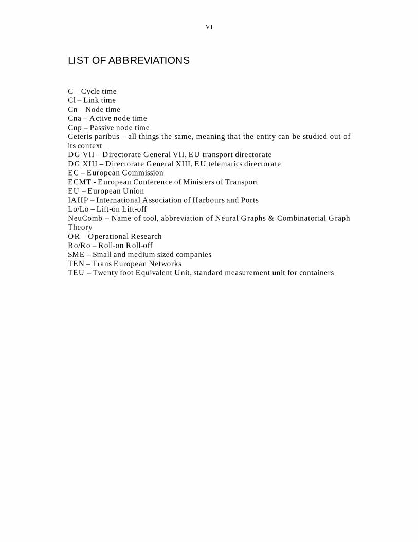
LIST OF ABBREVIATIONS C – Cycle time Cl – Link time Cn – Node time Cna – Active node time Cnp – Passive node time Ceteris paribus – all things the same, meaning that the entity can be studied out of its context DG VII – Directorate General VII, EU transport directorate DG XIII – Directorate General XIII, EU telematics directorate EC – European Commission ECMT - European Conference of Ministers of Transport EU – European Union IAHP – International Association of Harbours and Ports Lo/Lo – Lift-on Lift-off NeuComb – Name of tool, abbreviation of Neural Graphs & Combinatorial Graph Theory OR – Operational Research Ro/Ro – Roll-on Roll-off SME – Small and medium sized companies TEN – Trans European Networks TEU – Twenty foot Equivalent Unit, standard measurement unit for containers

VII

TABLE OF FIGURES Figure 1 Ultimate Presumptions → Paradigm →Methodological Approach ...............6 Figure 2 Methodological Approach → Operative Paradigm → Study Area ................7 Figure 3 Research approach...................................................................................................9 Figure 4 Reality – Model – Tool, interest area for Thesis ............................................. 10 Figure 5 Research workflow diagram................................................................................ 10 Figure 6 Phase I in the research work................................................................................ 11 Figure 7 Phase II in the research work.............................................................................. 11 Figure 8 Phase III in the research work ............................................................................ 12 Figure 9 The transport network, resources and infrastructure ..................................... 16 Figure 10 Network components.......................................................................................... 17 Figure 11 The network model ............................................................................................. 18 Figure 12 The logistics systems and its three subsystems............................................... 21 Figure 13 The port terminal as a network......................................................................... 22 Figure 14 Classification of systems..................................................................................... 25 Figure 15 The port terminal’s three foliated networks................................................... 27 Figure 16 Flow scheme for the optimisation .................................................................... 28 Figure 17 Efficiency figures for the current scenario...................................................... 30 Figure 18 Efficiency figures for the future scenario........................................................ 31 Figure 19 Complex dynamic logistics systems.................................................................. 37

VIII

1

1 INTRODUCTION This thesis is based on three years of research in close co-operation with ports and users in Europe within two EU projects EUROBORDER, sponsored by DG VII and INTERPORT sponsored by DG XIII. Five papers have been written three of, which are included, and constitute the thesis. The final result of the research is an optimisation and simulation tool called NeuComb/Port, which in all essential parts is built on information about the port terminals accumulated within the project and in close co-operation with the users. The main source of input comes from the analysis of problems and bottlenecks in the project and the definition of a functional port model. The name NeuComb is an abbreviation of Neural Networks and Combinatorial Graphs, on which the model/tool in some parts is based. 1.1 Problem background and relevance Short sea shipping plays a significant role in the European transport network. However, there is still much to be done to make it more competitive. (EC Green paper on Ports, 1998). The search for improvements is focusing on the ports as the interface between land and sea transport. The ports have been and still are an important but weak link in the transport chain, which gives great value to new ideas on how it is possible to change the port operations (Frankel, 1987). The traditional approach to enhance the efficiency of ports and port terminals has been to make large capital investments, either by new machines, expanding the area available for operation or hiring more labour. Currently there is a large pressure and competition among ports all around the world to become hubs for the different large shipping lines. The overall global trend in logistics is that there is a consolidation of goods in all different transport chains, but this is especially visible in the maritime sector. The European Commission among others has acknowledged this in their recent Green paper on Ports (EC, 1998) Another problem especially for the large hub ports, as for example Rotterdam and Hamburg, are heavy congestions and in particular there are problems getting the goods in and out of the ports. This is above all an infrastructure-related problem at the landside, creating bottlenecks and congestions in and around the larger ports. There are also problems with dwell times for vessels offshore but it is so far a smaller problem at least in Europe. In Southeast Asia e.g. Hongkong, Singapore and Shanghai this already is a problem. The small and medium sized ports on the other hand lack the operational efficiency of the large ports and are often situated at somewhat remote places with bad infrastructure connections to the main markets in Europe. The ports are currently the bottleneck in the international transport system, due to primarily two facts; firstly port management is a very traditional business

2

that adapts slowly to changes. The reason for this being the large costs associated with changes in the port terminal. There is also a basic difference in size between the trailers or trains feeding the port and the ships. This creates a necessary dwell time for the goods, simply because it takes time to accumulate the volumes necessary.1 The leading idea behind this thesis is that if the consolidation is continuing and there will be more and more goods exchanged at each port and each call, the throughput has to be enhanced. The other possibility is of course to expand the port terminal area, but this is not a realistic option in most cities since the port by tradition is located near the centre of the city. Some cities, like Helsinki, Bilbao, Hongkong, Los Angeles, to mention a few, are actually building completely new terminals outside the city to get rid of the problem. This is of course a very good solution, since it also handles the other problem namely the heavy traffic load through the city centres. It is, however, a very expensive solution and it takes a long time to build a port terminal from scratch. Therefore, the first option of trying to enhance the throughput is seen as a cheaper and more efficient solution especially in the short run. The relation between throughput time and land area needed is about linear, which means that if the throughput time can be halved, the land area needed can be halved too. This is ultimately the reason for the interest in advanced methods and tools for assessing the problem of terminal efficiency. There is a large potential of applying intelligent models and tools to the particular problems of designing the port terminal structure and use of the resources in the port terminal, some of which have been described above. This thesis concentrate on the problem of managing the port resources in a long-range view, e.g. the tactical and strategic level. Currently there exist few, if any models describing the port terminal from a pure network perspective (Ojala 1992, and references therein). In this thesis an optimisation and simulation tool is built that works with three foliated networks: an information flow network, a physical flow network and a set of resources constituting these networks. This relates closely to a conceptual framework developed for resources (Manheim, 1979). 1.2 Previous research This is a very brief recollection of some of the work done about simulation and optimisation of terminals and transport networks. This field has been quite extensively researched mainly in the context of Operations Research (OR). The most extensive research has probably been done at the Université de Quebec a Montréal, Centre de recherche sur les

1 To give a short example; a post-panamamax vessel carries around 6000 TEUs. To accumulate that volume in the terminal with a frequency of one trailer a minute takes 100 hours corresponding to circa 4 days and nights of an unbroken chain of trailers. To unload and load the vessel with a turnover rate of 160 TEU/hour which means 4 cranes working simultaneously, takes 75 hours corresponding to 3 days and nights of unbroken work. This totals 11 days of constant work to accumulate, load, unload and dispatch the containers.

3

transports. There a number of papers describing OR-algorithms for optimisation purposes and terminal and fleet management have been issued, the most prominent researchers being Crainic, Dejax and Gendrau. The group suggests that the container fleet management problem should be divided into two hierarchical levels – strategical/tactical and operational. The second level should be further divided into allocation, according to known and forecasted demand and routing of the transports of the containers (Crainic, Dejax and Delorme, 1989). They have worked with a lot of different approaches spanning from rolling horizon algorithms to using game theory and simulation techniques. In the area of simulation of seaport terminals Kondratowicz has done some interesting research (Kondratowicz, 1990, 1993). His work is concentrated to the area of simulation regarding terminals in general, for which he has developed a methodology. He has also developed a simulation tool called MULTIMOD, with which it is possible to simulate a seaport terminal. The problems of stochasticity in demand and system performance as well as the dynamics of network structures have been researched by Beaujon and Turnquist, acknowledging the difficulty with creating robust models as well as predicting demand (Hulthén, 1997). In a paper from 1992 Ojala describes different modelling approaches in port planning and analysis. He classifies them as three different approaches: econometric, analytic and simulation (Ojala, 1992). This classification was used in Paper I. In his book from 1987 about port planning, Frankel discusses and gives some valid thoughts about the importance of advanced methods, models and tools in order to, in an efficient way, assess the problem of planning and development of ports (Frankel, 1987). One of my senior colleagues at the department has also looked into the problem of simulation and optimisation of transport and logistic problems. In his dissertation Hulthén gives a broad view of the concept of container logistics and its management. He discusses the advantages and disadvantages of OR and more qualitative approaches. For a deeper insight is referred to his work (Hulthén, 1997). 1.3 Problem description and limitations In all sorts of terminal systems the resources operate on a network, sometimes according to a time schedule and on other occasions triggered by the arrival of a carrier of some sort e.g. a vessel or trailer. In any case there exists a problem in managing the resources, labour, machines etc. in the most efficient way. This thesis addresses the particular problem of optimising the use of resources within a port terminal, e.g. a Lo/Lo or Ro/Ro terminal.

4

From a logistic point of view the change or break of transport mode in a port, e.g. from rail or road to sea, causes substantial problems. These modes are at the same time quite different when it comes to capacity, which makes them even harder to integrate. This is especially true when the intermodal change is between sea transport and other modes. There is by default a waiting time (or build-up time) for goods that are to be transported by sea. This has been described more in detail in section 1.1 above. Every mode of transport and every large player, especially the large carriers, have their specific requirements on physical handling and information exchange facilities, which creates demands for true intermodality in the ports. There are a lot of definitions of intermodal, bimodal etc. The definition used here is the definition issued by the European Conference of Ministers of Transport (ECMT) since it is regarded as the most straightforward and useful of the definitions available (ECMT, 1993).

“The movement of goods in one and the same loading unit or vehicle which uses successively several modes of transport without handling the goods themselves in changing modes”

The ports are in the true sense integrated in the international transport chain, i.e. they are the main interface in international transport. Small and medium sized ports are particularly sensitive to changes and the new harder competition, since they have limited resources to implement the necessary developments and to go beyond their traditional role. This thesis assesses whether it is possible for small and medium sized ports to enhance their efficiency, without any large investments. There are a lot of terminals that work in a similar way as a port terminal when looking at the basic functions of the goods handling. The reason for choosing the port terminal as the object of study was twofold. The first being a very convenient opportunity to participate in a project aiming at enhancing port terminal efficiency for small and medium sized ports in Europe, and the other a personal interest in everything related to the maritime area. To assess the problem, three papers were written alongside the work in the project. The first paper (Paper I) outlines the basic framework for a model describing a terminal in general and a port terminal in specific. The second paper (Paper II) describes the functions and particular entities of the port terminal model, as being the drawing for the port terminal tool. The third and last paper (Paper III) describes the computerised port terminal tool, NeuComb/Port, that was built and some of the results from using the tool. For more detailed reading about the tool and the results, the reader is referred to the EUROBORDER project documents (EUROBORDER, 1998a, b). The limitations to this thesis are twofold. The first limitation is in the system studied, which has been limited to a single port terminal and its functions. The other limitations are that a quantitative perspective on modelling has been taken, when constructing the tool.

5

1.4 Purpose and scope The purpose of this thesis is fairly straightforward: Is it possible to enhance terminal efficiency without large capital investments? As it turned out this was a more complex and not that straightforward question after all, which will be obvious to the well-informed reader. The purpose can be further divided into three research questions:

• Can a port by modelling be treated like a generic terminal? •

What tools are needed to expand the flow in existing ports? • What limitations exist for this expansion and is there an upper limit?

These short questions have to be elaborated. The first question is basically assessing the possibility of treating a port as any terminal, because it would then be possible not only to model it but also to use ideas and other researchers’ results in that field. The second question is based on the need for further enhancements and increase of the flow (throughput of goods) through the terminals. The background is that currently the ports are the major bottlenecks in the intermodal chain, which has been described above. All ideas, models and tools that help us enhance the flow through the terminals will therefore be of great value. The third question is a consequence of the second one, and assesses the possible optimum and the absolute limit of these kinds of enhancements. To assess the purpose of the thesis, a theoretical model of a generic port terminal was built based on system and network theory together with Combinatorial Graph theory. This was then used as a base for a tool, called NeuComb/Port that was used to test several interesting cases relevant to the problem at hand. It should be pointed out that my personal knowledge of Combinatorial Graph theory is limited and there are others that have contributed to this part, which can be read in other papers (Jansen, 1998). The interested reader is also referred to the very extensive book on the subject written by Jungnickel (Jungnickel, 1994). The model was then developed into a computerised tool to be able to test different strategies and cases about port terminal efficiency.

6

2 METHODOLOGY This chapter addresses the issue of methodology, which consists of two parts; one addresses the presumptions about reality that this thesis is based on, which can be traced back to theoretical science. One addresses the actual handicraft of research, i.e. how the work was done. The chapter begins with a background presentation giving the reader the theories and the view of science on which this thesis is built. The end of the chapter has a more straightforward approach of giving the actual approach taken. The approach followed is a very pragmatic one, concentrated on understanding and applying the theories as described in different books about methodology. The in-depth penetration of methodology and theory of science has to be postponed to my doctoral thesis. 2.1 Theory of Science - Methodology A lot of factors, such as history of the field, basic assumptions about the reality, language etc. influence the way a researcher remains true to the subject of study. The importance of this is pointed out by Arbnor and Bjerke (1997) saying that we can hardly understand the data collected and try to understand and explain anything, if the researcher has not considered how the particular approach will shape the observations, understandings and explanations. Hence it is also clear that to be able to say anything at all about anything we have to take a stand on something, a platform of believes. These presumptions will affect everything that the researcher will do from choosing the subject to the recommendations made. This can be illustrated as in Figure 1 and Figure 2.

UltimatePresumptions

MethodologicalApproach

Paradigm Theory of Science

Figure 1 Ultimate Presumptions →→→→ Paradigm →→→→Methodological Approach (Arbnor&Bjerke, 1997)

The ultimate presumptions are our basic view on the world, for example that it is round and not flat. This has to do with philosophical ideas about our conception of the reality is actually constructed, and is foremost studied in the theory of science. Already Plato elaborated on this in his discussion about the world. However any deeper discussion about this is out of the scope of this thesis, but two more things have to be added since they constitute the idea. The

7

first is the concept of science that has to do with the way we have been taught and gained knowledge in our education. This obviously has an impact on how we approach problems in science. The second thing is scientific ideals that also influence the researcher, especially in choosing the area of study. The concept of paradigm was originally minted by Kuhn (1970)2 and describes the “ruling” view within a certain branch of science or the whole community, as the example with the world mentioned above. Kuhn argued that paradigms only shifted “violently” by a “revolution” of the young paradigm against the old ruling one. Finally there is the methodological approach which basically means the concept of how mankind builds knowledge.

MethodologicalApproach

StudyArea

OperativeParadigm Methodology

Figure 2 Methodological Approach →→→→ Operative Paradigm →→→→ Study Area (Arbnor&Bjerke, 1997)

The methodological approach is then transferred to an operative paradigm, which is actually the working method and approach used in the specific research. The operative paradigm is influenced by the methodology “tool-box”, e.g. the different methodologies possible to use regarding the specifications of the studied area of the reality. Most often there are methods more or less suitable for a specific research question and study area. There are three different methodological approaches, the Analytical approach, the Systems approach and the Actors approach (Arbnor&Bjerke, 1997). These approaches will be briefly described as a background to the basic approach taken in this thesis and as a link to the paradigm and method used which will end this chapter. The Analytical approach is what can be called the classical natural science approach. The reality is seen as independent from the observer, scientist, and conformable to “laws of nature”. The science is based on the assumption that the parts make up the whole and as long as the parts are described well enough the scientist merely has to put them together to get the whole picture. The knowledge is not dependent on individuals and parts can be explained by verified facts. The aim and the results the scientists strive for are causal relationships and ultimately laws of nature. 2 Here cited from Arbnor and Bjerke

8

The Systems approach was a reaction to the analytical approach and emphasises that the reality consists of mutually dependent systems. The best-known systems approach word is probably “synergy”, which means that the sum is not equivalent to the parts. This approach is dominating in social science today. All knowledge is according to this approach system-dependent or if preferable context-dependent. This means that the systems approach explains the parts out of a holistic approach. The aim and result the scientist strives for is to create logic models and representative cases. To build models of the systems as a way of explaining and understanding the reality is a basic feature in this approach. The Actors approach was in its turn a reaction to both the others and emphasises that the reality is a social construction, which does not exist independently of the scientist. As soon as we want to study something we interact with the studied object and in that sense influence the results. The actors approach, as opposed to the two others, has not as a main objective to explain how something works, instead the main issue is to understand social constructions. All knowledge is individual-dependent and both the scientist and the “object” will interact and learn something new. The whole is understood via the actors’ images of the reality. In this approach the scientists search for typical, descriptive cases for a class of systems. The scientists try to develop a descriptive language so as to be able to discuss different specific situations and to transfer knowledge in the whole community. A common technique is the dialectical interview. This thesis is built upon the systems approach and systems science together with the views of Cybernetics. (Cybernetics is, in short, the theory of automatic control please refer to chapter 4 for a more detailed discussion). The reason for this approach is the firm conviction that the various parts of reality are linked together and can only be understood by a holistic approach. It is also a consequence of a preference for using models of different kinds as a way of explaining thoughts and ideas. The approach taken is though not “classic” in the sense that the reality necessarily by itself is considered as being a system, but that it is a very convenient and strong metaphor. The notion of inevitable interaction between the scientist and the area of study is also taken into consideration, since this thesis in itself is proof of that. The handicraft of science is cyclic and therefor the moment of interaction and mutual dependence is inevitable. The knowledgeable reader will notice influences from all the different approaches by the language used. As a result there is a mix of analytical, systems and actor “words”. However the basic view is consistent with the systems approach. 2.2 Research approach – method used Since this thesis is based on three years of work with European ports it has been possible to test ideas and models continuously against what is contained in the triangle in Figure 3 below. The collective knowledge and industrial applications in this specific case consists of the knowledge of the member ports in the project, Helsinki and Rauma in Finland, Piraeus and Thessaloniki in

9

Greece, Oslo in Norway, Bilbao in Spain and Gothenburg in Sweden. These ports have provided the main influences but also other ports in Europe (Rotterdam, Antwerp), North America (Port of Los Angeles) and Southeast Asia (Singapore, Hongkong) have given inputs and shared their thoughts on the issue. By interacting with these ports the research has been redefined and refined several times, although the basic approach and research problem has been consistent. The systems context describes the knowledge of the senior colleagues of the department and all the literature in systems science, methodology, networks theory and articles that have helped defining the area of research. The analytical contribution (that should not be regarded as being based on the analytical approach) is the 5 papers written about port terminal efficiency and how to model port terminals in an adequate way.

Visible to industry

IndAppl

Sight depth

Analytic contribution

Collective knowledge

Individual knowledge

Systemscontext

Figure 3 Research approach (Applied from Sjöstedt)

A note about research in different context can be in its place here. Re and search stands for recreating something, which goes back on the analytical approach. The reality is of God created and our work as scientists is to try to recreate how this was done, and if we succeed we can add another law of nature to the pile that already exists. This is all well in the classical sciences of physics and so on, but in social science where transport and logistics in the broader sense has to have its place as a genuine interdisciplinary science, this is somewhat difficult. Applied sciences try to create something new to add to our basic knowledge rather than to recreate something that already exists. It is out of the scope of this thesis to discuss this at length but one should notice that this has a major impact on the notion of validity and validation of theories. If something new is created, against what are we then supposed to validate it? What is then our point of reference?

10

2.2.1 Method The method is based on the research area that has been the focus of the project and this thesis which considers the interface between the reality, that had to be described, and the tool describing the reality as well as possible. This is shown in Figure 4.

Figure 4 Reality – Model – Tool, interest area for Thesis

The figure tries to describe the difference and interaction between the reality, the theoretic model and the computerised tool. It also shows the area of study, correspondent to the interest area of this thesis. The approach has as mentioned before been pragmatic, which is described in Figure 5 below that, in a more formal way, tries to describe the workflow of this thesis.

Figure 5 Research workflow diagram

The research as such went through three phases as described in Figure 5 above: Phase I, which was explorative, Phase II which was descriptive and designing the tool, and finally Phase III that was deriving the results. The approach in this thesis has been holistic in the sense that an attempt has been made to give the whole picture of which the three different papers (see paper I-III) only give parts of the information.

Literature research

Thesis

Feedback

Case study

Model Tool Results

Feedback

Feed forward Feed forward

Phase I Phase II Phase III

Case study

Literature research

Reality Model Tool

Area of study

11

2.2.2 Explorative phase The explorative phase began immediately after the project had been started, by doing a quite extensive desk research the area of study was scanned for valid information. The methodology is schematically described in Figure 6 below.

Figure 6 Phase I in the research work This was done by assessing different databases at the libraries and by using Internet to search for references to articles and other interesting publications. Databases searched were among others COMPENDEX (Science & Engineering), ABI/INFORM (Business and Industry) for articles and CHANS (Chalmers University Library database) and GUNDA (Gothenburg University Library database) for books. This can be referred to as a literature survey, which is done just to establish a frame of reference (Hellevik, 1977). Together with this, a case study and a mail survey, where made in the project, from which results and issues were extracted. For more information about the mail survey is referred to the EUROBORDER project (EUROBORDER, 1997). This resulted in Paper I, describing the basis and thoughts behind using the network concept for modelling a port terminal. 2.2.3 Descriptive and design phase The descriptive phase was strongly interrelated with the explorative phase as shown by the feedback and feed forward loops in Figure 7.

Figure 7 Phase II in the research work

Literature research

Feedback

Case study

Model Tool

Feed forward

Phase I

Tool Results

Feedback

Feed forward Feed forward

Phase II

Case study

12

Since the model was the base for the actual computerised tool, this phase had to be more descriptive giving the different interrelations and parameters that could be used for implementing the theoretic model into a working tool. The main work in this phase was to define and describe the actual parameters that could transfer the reality to a model, actually valid to use as a base for a computerised tool. This was done as a case study, assessing the problems and special structures of the different port terminals participating in the project. The goal was to have such a good view of the different terminals, so as to be able to assess what parameters were especially sensitive, and therefore had to be included, and which were expandable. These kinds of tools are purely quantitative why choosing relevant parameters and design of the tool is very essential (Kondratowicz, 1990). This work resulted in Paper II, which is a fairly comprehensive paper describing the tool, the working interface as well as how to work with the tool. 2.2.4 Result phase The last phase consisted of the practical work of adjusting and readjusting the tool together with the final users, i.e. planning managers of the port terminals. This was an extensive work since the port terminals differed quite a bit regarding their organisation and the handling of the goods. The iterative work is shown by the second feedback and feed forward loops in Figure 8, since the results implicated changes in the tool repeatedly.

Figure 8 Phase III in the research work At the same time a few representative and interesting cases were created to test the potential of the tool and this kind of approach to modelling and assessing the problem. This work resulted in Paper III describing some of the results from running the tool, primarily at the port terminal of Ormsund, Port of Oslo, Norway. Finally, in this phase, a second literature survey was made to assess the latest articles and publications in the field.

Thesis Results

Feed forward

Phase III

Literature research

13

2.3 Method and validation of simulation and optimisation In this section a short description of the method used for the simulation and optimisation together with the validation of the actual tool is included. The reason is that it is seen as an integrated part of the thesis although not central. 2.3.1 Method The method used for the development of the NeuComb/Port tool was straightforward containing 4 steps. •

Development of a theoretical model as base for the tool • Development of a mathematical model •

Implementation of the model into a computerised tool • Testing, validation and reiteration This approach is comparable to the process of quantitative analysis described in “Principles of Operations Research” (Wagner, 1975) The approach is divided into four stages. Formulating the problem, which contains which variables that are controllable and which are not, the basic structure of the problem etc. Building the model, which is to decide in detail what simplifications to make and identify the dynamic as well as the static structural elements. Performing the analyses, in this part the mathematical solution to the problem is calculated. As pointed out by Wagner there is always a risk of formulating the model to complex or to simplistic, why the approach is iterative in its implementation. The final phase is implementing the findings and updating the model, this part is very essential since it is highly unrealistic to believe in a step-to-step solution where nothing is going wrong or simply has to be redone due to misinterpretations of the formulated problem 2.3.2 Validation This short introduction outlines the rationale behind the validation approach. The work done validating the soundness of the NeuComb/Port tool was based on the principle of simplicity. The rationale behind the approach was to build a simple model with a supposedly simple and predictable behaviour, and to check that this model behaved as expected. This test was a matching of behaviour against the intuition of the domain expertise within the group, in particular the Oslo Port Authority. The model used to check was a model of the Ormsund terminal of the Oslo Port. (EUROBORDER, 1998d) The validation considered only time simulation and optimisation, as cost data were at best crude approximations. as a consequence only ordinary cargo types, and no special handling of reefer or dangerous goods were used. A more formal approach could start out by showing the correctness of the algorithm, by deducing an invariant for the algorithm, proving that the algorithm preserves

14

the invariant, and then to show that the invariant leads to a fix point, in which the solution is reached. Another, possibly complementary approach, could be to generate a representative selection of models samples, and then, by statistical means, showing that the expected behaviour correspond to the actual behaviour, i.e., that hypotheses predicting specific results were confirmed. The problem of delineating the borderline between testing the tool and testing the actual models would then have to be addressed. The issues mentioned above concerns all formal verification of software systems, and particularly simulation software. (EUROBORDER, 1998d) Due to the highly complex technical nature of these approaches, compared to the relatively modest resources this more down-to-earth approach was chosen. 2.4 System boundaries - criticism The system boundaries were more or less automatically decided to be the port terminal since that is the most suitable entity in the port for building a model around. In most ports the port terminals are very self-dependent, especially when talking about Lo/Lo and Ro/Ro terminals handling container and trailer traffic. They are normally seen as an entity of their own, dating back to the formation of the ECT terminal in Rotterdam in the mid-sixties, which was set up by a number of Rotterdam stevedores at the instigation of the Municipal Port Management, as a dedicated container terminal. It was decided to include the physical handling, the resources in the system as well as the information systems and administrative routines in the model. This was due to the fact that the project was aiming at enhancing port terminal efficiency by assessing organisational, administrational and information issues. In retrospective this was perhaps a little too much and we had to rethink the original design in a couple of steps. One of the shortcomings of this thesis was the ambition to place my own research in a context of all other research done in this area, methodological as well as from the practical research perspective. There is no option but to admit that this goal has not been possible to reach and that it has to be deferred to the doctoral thesis. Since most of the work has been performed during the last three years and published in papers along the way, a certain redundancy between especially chapters 3 and 5, and the papers is inevitable but hopefully this does not disturb the reader more than necessary.

15

3 FRAME OF REFERENCE This chapter is an extension of the frame of reference that is primarily described in Paper I-III. It was considered necessary to extend and enhance the frame of reference that this thesis is built on after the second literature review in phase 3, described in section 2.2.4. 3.1 Transport networks and terminals The work in this thesis is based on two fields of science, one being the theory of networks, which describes transport systems as being networks. The other field is systems science that is described in chapter 4. The network as a metaphor is widely used and has because of its extensive use also become less precise in its definition. Therefore this chapter begins with a description of three different ways of using the network metaphor: the network as a transport metaphor, the Network approach according to the Uppsala school and mathematical networks. 3.1.1 The network as a transport systems metaphor A network basically exists of nodes and links describing an interconnected web which is a very good metaphor for both transport networks and terminals. This is a common theory base that is used at the Department of Transportation and Logistics. Wandel and Ruijgrok make the basic notion of networks and the correlation between the description of the transport industry as a network very clear in their paper (Wandel & Ruijgrok, 1995). The correlation between the infrastructure, the resources that move on the infrastructure and constitute the transportation network is shown in Figure 9. The figure describes the correlation between the aggregation level and the components of the system and the markets. The traffic is regarded as a market for infrastructure services, e.g. the trade of space and time. Transport is the market for the movement of vehicles on the infrastructure. The accessibility market are the market for flows (or slots) made available by the service providers operating on the transport market. Finally there is a market for functionality that is derived from the producer and consumer relations. The consumers buys (with money or equivalent) articles that gives the users a certain kind of functionality. The model could possibly be expanded to include the financial market including the macro economic scale but it was not regarded as useful to expand the model that far in this context.

16

Flows

Vehicles

Infrastructure

TRANSPORT

TRAFFIC

MICRO

MACRO

AGGREGATION MARKETS

Articles

Money

ACCESSIBILITY

FUNCTIONALITY

$

$$

$

$

$

$ $

P

PP

P

P

P

P P

COMPONENT

Figure 9 The transport network, resources and infrastructure (Wandel & Ruijgrok, 1995), (Here adapted and modified from Lumsden 1999)

A network consists of nodes and links and there are at least two ways of describing networks. One is that the network consists of nodes and links, where the nodes correspond to an activity performed and a halt of the flow in the network and all movements are represented by links (Lumsden, 1998). The other describes the nodes as just being intersections or states and all movement and handling is done in the links. The main difference between these two ways of describing a network is that in the first case the activity creates an added value, which does not exist in the second case.

17

C

C

Node

Link

Cycle time

A B

Figure 10 Network components

On the network, described in Figure 10 above, the goods and resources are moved according to specified routes. The time or capacity for a node or a link can be different which means that the network has to be configured with the parameters constituting it. One way of doing this is to describe the network by the cycle time as shown in Figure 10. The cycle time ( c ) can be divided into

link time ( lc ) and node time ( nc ), the link time describing the part of the time necessary to perform the transport or movement of goods from one address to another. The node time can in its turn be divided further into active node time ( nac ) and passive node time ( npc ). The active node time consists of the time it

takes for handling the goods in the node and the passive node time is the time the goods are stored without any handling. (Lumsden, 1995). A network can also be described as a physical network or an abstract network. The physical network is the actual infrastructure where the goods and vehicles are moving. The abstract network is the “trade network” meaning the O/D matrices building up the connections between for example suppliers and retailers, which is shown by the O/D pair A and B in Figure 10 above (Lumsden, 1995). There are other definitions of the same concept referred to as a cycle in this thesis, but the definition above is regarded as a straightforward and easy to convey one, why it has been chosen. The different topics captured by the network model are another way of describing it (Magnanti and Wong, 1984).

“Indeed, network design issues pervade the full hierarchy of strategic, tactical and operational decision-making situations that arise in transportation.”

3.1.2 The network approach according to the Uppsala school The Network Approach to studies of market structures was developed at the University of Uppsala and the Stockholm School of Economics together with researchers from other countries within the framework of the Industrial Marketing and Purchasing group (IMP). Key researchers in the development of

18

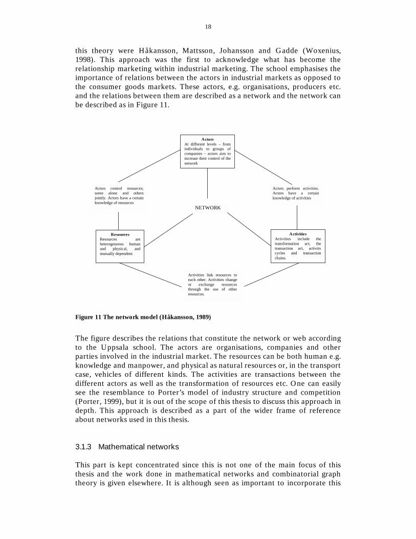
this theory were Håkansson, Mattsson, Johansson and Gadde (Woxenius, 1998). This approach was the first to acknowledge what has become the relationship marketing within industrial marketing. The school emphasises the importance of relations between the actors in industrial markets as opposed to the consumer goods markets. These actors, e.g. organisations, producers etc. and the relations between them are described as a network and the network can be described as in Figure 11.

ActorsAt different levels – fromindividuals to groups ofcompanies – actors aim toincrease their control of thenetwork

ActivitiesActivities include thetransformation act, thetransaction act, activitycycles and transactionchains.

ResourcesResources areheterogeneous humanand physical, andmutually dependent

Actors control resources;some alone and othersjointly. Actors have a certainknowledge of resources

Actors perform activities.Actors have a certainknowledge of activities

Activities link resources toeach other. Activities changeor exchange resourcesthrough the use of otherresources.

NETWORK

Figure 11 The network model (Håkansson, 1989)

The figure describes the relations that constitute the network or web according to the Uppsala school. The actors are organisations, companies and other parties involved in the industrial market. The resources can be both human e.g. knowledge and manpower, and physical as natural resources or, in the transport case, vehicles of different kinds. The activities are transactions between the different actors as well as the transformation of resources etc. One can easily see the resemblance to Porter’s model of industry structure and competition (Porter, 1999), but it is out of the scope of this thesis to discuss this approach in depth. This approach is described as a part of the wider frame of reference about networks used in this thesis. 3.1.3 Mathematical networks This part is kept concentrated since this is not one of the main focus of this thesis and the work done in mathematical networks and combinatorial graph theory is given elsewhere. It is although seen as important to incorporate this

19

part as a complement to the other definitions. Network theory is a very efficient tool to be used as a base for describing a port terminal. In this section the ideas and theory of networks coupled to the frame of reference is given. A network can be defined as nothing more (or less) than a system (Casti, 1995):

network objects connections system= + =

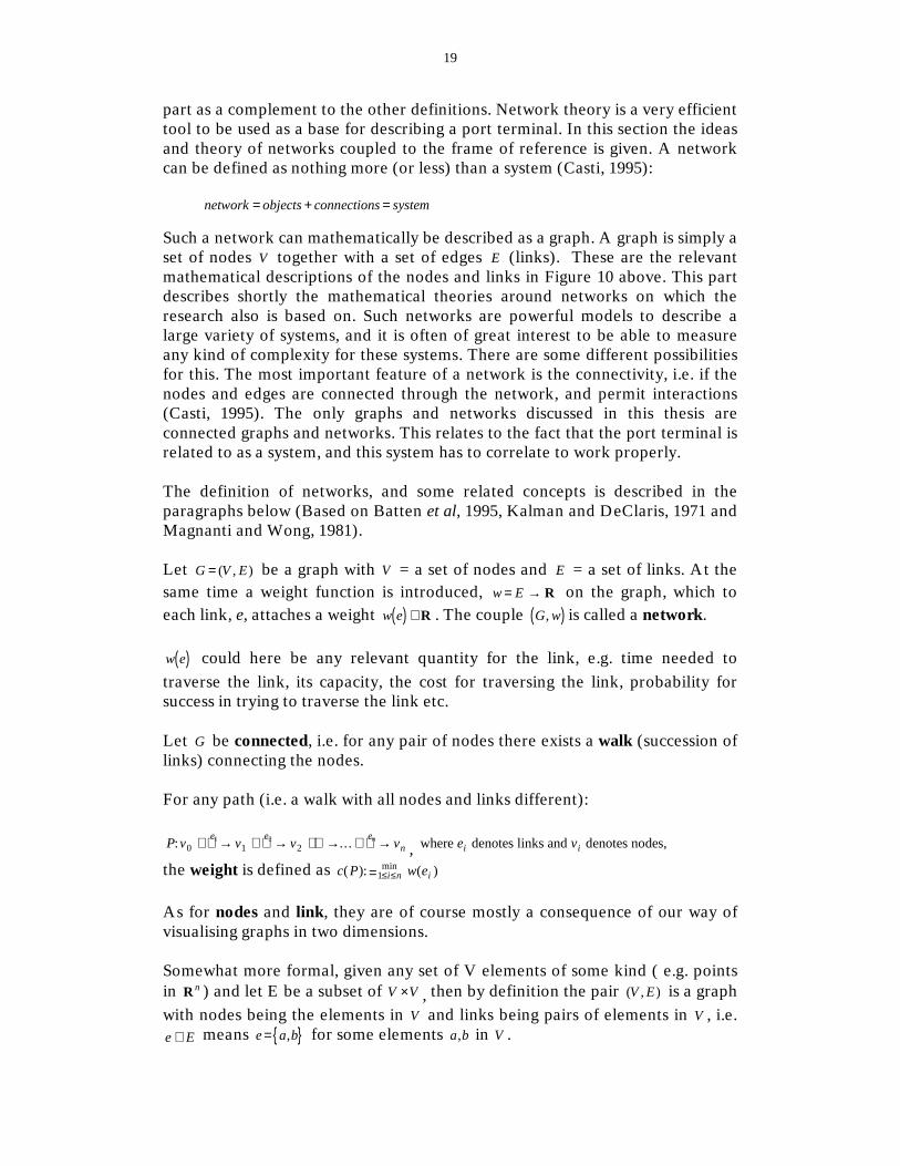
Such a network can mathematically be described as a graph. A graph is simply a set of nodes V together with a set of edges E (links). These are the relevant mathematical descriptions of the nodes and links in Figure 10 above. This part describes shortly the mathematical theories around networks on which the research also is based on. Such networks are powerful models to describe a large variety of systems, and it is often of great interest to be able to measure any kind of complexity for these systems. There are some different possibilities for this. The most important feature of a network is the connectivity, i.e. if the nodes and edges are connected through the network, and permit interactions (Casti, 1995). The only graphs and networks discussed in this thesis are connected graphs and networks. This relates to the fact that the port terminal is related to as a system, and this system has to correlate to work properly. The definition of networks, and some related concepts is described in the paragraphs below (Based on Batten et al, 1995, Kalman and DeClaris, 1971 and Magnanti and Wong, 1981). Let G V E= ( , ) be a graph with V = a set of nodes and E = a set of links. At the same time a weight function is introduced, w E= → R on the graph, which to each link, e, attaches a weight ( )w e ∈ R . The couple ( )G w, is called a network.

( )w e could here be any relevant quantity for the link, e.g. time needed to traverse the link, its capacity, the cost for traversing the link, probability for success in trying to traverse the link etc. Let G be connected, i.e. for any pair of nodes there exists a walk (succession of links) connecting the nodes. For any path (i.e. a walk with all nodes and links different): P v v v ve e e

nn: ...0 1 2

1 2 → → → → , where e vi i denotes links and denotes nodes,

the weight is defined as c P w ei n i( ): ( )min= ≤ ≤1 As for nodes and link, they are of course mostly a consequence of our way of visualising graphs in two dimensions. Somewhat more formal, given any set of V elements of some kind ( e.g. points in R n ) and let E be a subset of V V× , then by definition the pair ( , )V E is a graph with nodes being the elements in V and links being pairs of elements in V , i.e. e E∈ means { }e a b= , for some elements a b, in V .

20

Drawing the graph ( , )V E , { }e a b= , is of course identified as the straight line, ”link”, between a and b. 3.1.4 Summary and approach taken in the thesis The approach to networks taken in this thesis is clearly correspondent with the network as a transport systems model, described above. Some parts of the other approaches are used as a frame of references and as a complement to the main approach. The Uppsala school network approach is very useful to describe the qualitative effects in a transportation system, and the definition of a network by Casti is regarded as very elegant and to the point why it is used as the base definition of a network. Here repeated.

network objects connections system= + =

The objects are regarded as the nodes in the transport system, e.g. terminals in the large system and storage areas in the context of terminals, as used in this thesis. The connections are the links/roads between the terminals or within the terminals between the different storage and transfer areas etc. There is still a problem of assessing the different networks, information, physical and resource, in the same model and tool. One of my senior colleagues at the department a model has developed a model that is coping with this problem in an elegant way that is described in Figure 12 below. In this model, which resembles Figure 9, there are three levels. The higher levels always containing the lower levels. The general level is called the abstract system and contains all activities seen as economic activities. This corresponds to the OD networks in Figure 9 and Figure 10. This flow is abstract in the sense that the flow is not physical, rather it is economic and legal transactions. It is also mapping the relations described in Figure 11, since this level is purely descriptive. This system is then transformed down to the information, or virtual system, which transforms the relations and transactions into a virtual network describing the actual components of the system. The physical system is contained in the virtual system, since the physical components, the resources etc. are seen as parts of information building the virtual system. The lowest level is the physical level which contains the infrastructure and the resources as seen in most models.

21

(transaction)

Information SystemVirtual System

Physical System

Abstract SystemEconomic Activities

Physical System

Indicators/criteria for

economic efficiency

(transaction)

“Information”

(transaction)

Physical Flow

Information Flow

Abstract FlowAccessibility System

Transportation System

Logistics System

Figure 12 The logistics systems and its three subsystems (Carlsson, 1999)

It is possible to expand this model to include the traffic system with the resources and then connect it tighter to the model shown in Figure 9. This is though out of the scope for this thesis. The approach taken in Figure 12 corresponds to the approach taken in this thesis and the approach that was taken in the project as a base for the NeuComb/Port tool. The reason being that all parts of a system, infrastructure, resources information etc. are described by parameters enabling us to build a computerised tool of the network and mathematical models used. As a consequence the computerised tool will handle all networks at the virtual level, and they will all be transferred to the same level avoiding the problems of handling information and physical networks in the same model or tool. The network design is very important for the actual model, and what it is supposed to be modelling. The model serves as a base for both a vehicle routing problem, i.e. how the flow is going through the network, and a facility location problem, i.e. the network lay-out. There are possible interactions in both the links and the nodes. This means that a combination of the two most common ways of describing a network is done. A network is described as a combination of nodes connected by links. Either the nodes are characterised by parameters or the links are only connecting them, or the nodes are only expressing the

22

topology of the network and all other characteristics are associated with the links as described above.

R/D

T S L/U

I1 I2 R1

CargoType 1 IN

CargoType 2 IN

= Cargo

= Information

= Resource

CargoType 1 OUT

CargoType 2 OUT

R/D

T

T

T

T

T

T

S R/D

= Transfer

= Storage = Receive/Delivery

L/U = Load/Unload

SEASIDELANDSIDE PORT TERMINAL

Nodes Areas Functions

Figure 13 The port terminal as a network (Waidringer & Lumsden, 1997)

Figure 13 shows an example of how to describe a port terminal, with a network model. It serves as an applied example to the theory described above. It is of course possible to make this model much more complex, but to make it fairly easy to describe and discuss, no other nodes, links and resources have been added than those described above.

23

4 SYSTEMS SCIENCE AND CYBERNETICS Systems science and cybernetics have strongly influenced this thesis’ view of reality and therefore the two interrelated science fields have been given a separate chapter. Research about transportation and logistics is a truly interdisciplinary subject why it is often useful, not so say necessary, to search for theories from other fields. Working with the project and this thesis led to contact with systems science and the notion of cybernetics, which both were perceived as good complements to network theory to complete the structure of this thesis. By using networks to explain and model port terminals, the work is already headed in the direction of systems science, since an interconnected network by definition is a system. 4.1 Systems science Systems science is based on the notion of the reality being possible to describe as a system, and that it is possible to understand the parts from studying the whole system. It is systems science that has given us words and expressions as “synergy” “2+2 ≠ 4 (Arbnor and Bjerke, 1997). It was originally an attempt to go beyond the analytical approach, which was and still is the dominating approach in all natural sciences, as for example Physics. To give an example of the power of systems science, think about Ohm’s law “U=RI”. This law is not applicable at the atomic level but instead its strength is just that it studies the problem from an aggregated systems level and therefore can provide accurate answers for a whole set. This example originates from mathematical statistics and is therefore not primarily connected to systems science, but all the same a good example of what systems science is all about. Analytical findings at various levels of resolution in for example physics can only be understood simultaneously in a systems context. This approach corresponds in all important parts with the earlier stated view of how the reality is constructed.3 The importance of taking a holistic approach cannot be emphasised enough when dealing with complex dynamic systems like terminals and transportation and logistic systems. Even though the notion of systems science is not new, there have been references to the old Greeks as being the first. It is commonly considered that von Bertalanffy with his research in the 1940’s is the father of modern systems science. He was using the systems context in his biological area and developed a theory based on this research (von Bertalanffy, 1968). Otherwise there are two scientists that are both intimately connected with the systems science, Checkland and Churchman have both contributed to the context of systems science. Checkland is discussing systems science out of the basic structure used by von Bertalanffy, but he concentrates on how to create a common language and understanding about what the systems science approach is really signifying and how it can be used in everyday practice by the scientists (Checkland, 1981). 3 See discussion in the preceding chapters

24

Churchman has contributed, among other things, with a five basic beliefs that the scientist keeps in mind when thinking about the meaning of a system (Churchman, 1981) He made this list as a help in defining and thinking about systems and what constitutes them.

•

The total system objectives and, more specifically, the performance measures of the whole system

• The system’s environment, the fixed constraints •

the resources of the system • the components of the system, their activities, goals and measures of

performance •

the management of the system One may distinguish between two aspects of the systems approach: efficiency and necessity. Efficiency meaning that in the analysis of complex systems the systems approach is more efficient than reductionistic, necessity meaning that the approach is necessary because reductionistic analysis is incorrect, no matter how detailed the analysis (Hulthén, 1997). One of the main problems when performing research on large transport systems is the complexity of the industry. If the research efforts are too specific it easily leads to suboptimisation since a ceteris paribus approach is not suitable for analysing the individual components. An aggregated systems approach is thus a prerequisite, together with a profound knowledge of the industry at study, for researchers who want to achieve scientifically reliable results. (Woxenius, 1998) One of the cornerstones of the systems science approach is models and how to construct them in a meaningful way. Often the reality we want to describe is of such magnitude or connected in so many ways that we cannot map it by just transferring the reality directly, and thus it is most useful to create a model of the real system. The model is by default a simplification of the real system (otherwise it would be the real system in itself and we would have gained nothing) and the main skill and purpose is to make the transcription to a model as well as possible. It is therefore important to identify the main characteristics of the real systems so as to incorporate them into the model. It is also crucial to test the model for sensitivity since it is a well-known fact that there are always some aspects (parameters) of the reality that will influence the model more than others. It is possible to distinguish between isomorphic and homomorphic models. An isomorphic model from the real system is a one-to-one transformation, e.g. each characteristic in the real system is transferred to the model. When dealing with complex or large systems it is often necessary to simplify the model and make a many-to-one transformation, meaning that characteristics from the real systems are grouped together and being represented by a single parameter in the model. The last model is a homomorphic model (Hulthén, 1997). This is often the case when dealing with any real system of some magnitude.

25

4.2 Cybernetics The field of cybernetics was in a sense born with the interdisciplinary group of scientists that gathered around Wiener, just after World War II. They were all interested in control theory but from different perspectives, and fields of research, but they acknowledged the similarities in their problems. This section though starts with two cites from Beer (Beer, 1959)

“Cybernetics is the science of communication and control”

“Cybernetic systems are exceedingly complex, and their controls cannot be defined in specific detail”

These cites are seen as essential as a definition of cybernetics and an explanation of why the science of cybernetics, is regarded as so interesting as a frame of reference in this thesis. The approach taken is perfectly in line with the thoughts of cybernetics (although this was not fully understood at the time the subject was chosen). The research problem considers if it is possible to use advanced methods and tools for solving management and control problems. Beer also classifies systems according to if they are deterministic or probabilistic and their level of complexity as shown in Figure 14.

SYSTEMS Simple Complex Exceedingly complex

Deterministic Window catch Computer Empty Billiards Planetary systems Machine-shop lay-out Automation Probabilistic Penny tossing Stockholding The economy Jellyfish movements Conditioned reflexes The brain Statistical quality control Industrial profitability The Company

Figure 14 Classification of systems (Beer, 1959)

In Wieners book about cybernetics (Wiener, 1948) he describes the work and findings that he and the group of scientists around him had completed so far. It gives insights into several fields of science, since the group was very heterogeneous and only used cybernetics as a tool for research in their respective area of research. It should though be read with the history in mind, since a lot of their hopes have exceeded their wildest expectations and others have proven not to hold. The reader might think that it is a waste of time trying to use “old” knowledge since a lot of the expectations, after all, have been put to rest indefinitely. The latest advances in mathematics methods and computer science, though, imply differently. With today’s enhanced tools and methods, cybernetics offers an interesting field of thoughts to investigate. Another prominent scientist in the field is Ashby that in one of his publications provides a very good introduction to cybernetics (Ashby, 1956). In this book he gives a very thorough survey of cybernetics, but his major contribution is the “law of Requisite Variety”, which says that in order to control a system the control mechanism must mirror the variety of the real system. This is a very

26

useful law to classify systems and for building control and regulating systems. The chapter about systems science and cybernetics is intentionally kept short but is regarded as essential to the thesis, since it presents the fundamental thought behind the research, on which this thesis is built.

27

5 SUMMARY OF APPENDED PAPERS

5.1 Research basis for the papers Here a citation, a shared favourite by a senior colleague of mine and myself, has to be included, since I feel that it is most appropriate to quote Stafford Beer in (Beer, 1985):

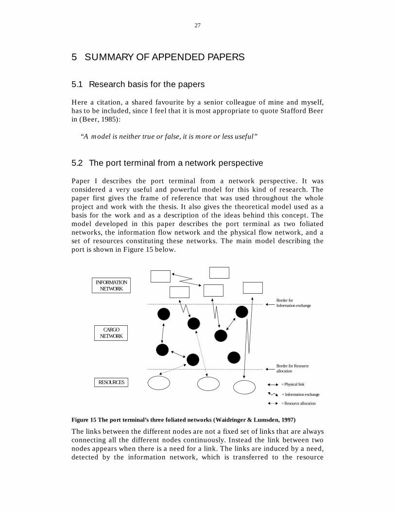
“A model is neither true or false, it is more or less useful” 5.2 The port terminal from a network perspective Paper I describes the port terminal from a network perspective. It was considered a very useful and powerful model for this kind of research. The paper first gives the frame of reference that was used throughout the whole project and work with the thesis. It also gives the theoretical model used as a basis for the work and as a description of the ideas behind this concept. The model developed in this paper describes the port terminal as two foliated networks, the information flow network and the physical flow network, and a set of resources constituting these networks. The main model describing the port is shown in Figure 15 below.

INFORMATIONNETWORK

CARGONETWORK

RESOURCES

Border forInformation exchange

Border for Resourceallocation

= Physical link

= Information exchange

= Resource allocation

Figure 15 The port terminal’s three foliated networks (Waidringer & Lumsden, 1997)

The links between the different nodes are not a fixed set of links that are always connecting all the different nodes continuously. Instead the link between two nodes appears when there is a need for a link. The links are induced by a need, detected by the information network, which is transferred to the resource

28

network. After that a resource, i.e. a machine, personnel etc., is assigned to solve that need, by creating the desired link. The status from the physical network is transferred to the information network. This network detects the need and assigns a resource, creating the link, for that need. In the information network information is also sent to the next node corresponding to the physical node receiving the goods. 5.3 Simulation and optimisation of a port terminal Given in Paper II is the basis for the NeuComb/Port model and tool. The program is an implementation of mathematical algorithms adjusted to a port terminal environment. The NeuComb/Port tool is a theoretical research tool ready to use and adjust to the situations in different port terminals. Paper II is in all essential parts built on the first paper and shares the same frame of reference and view of reality. This paper describes the decision made when designing the tool and gives a detailed description of the tool. All the different functions and possibilities with the tool are described as well as the limitations that necessarily are connected to these kinds of tools. The model works as follows:

• Simulation of the physical and information flows • Optimisation of the physical and information flows •

Optimal matching of the resources under the boundary constraints

Scanning thesystem

Free flowoptimisation

Optimalassignment

Resourceallocation

Scanning thesystem

Figure 16 Flow scheme for the optimisation (Waidringer & Lumsden, 1998)

To show the principle method of the optimisation Figure 16 is incorporated. The tool works in the following way; first the system is scanned for input about the status of the system, and after that the free flow optimisation part is performed. When this is done a new scan of the system is done for the assignments to be performed and after an optimal assignment and resource allocation the cycle is completed. The approach taken above is seen as a very useful one, since it creates a way around a both, practically and theoretically, unsolvable problem. The notion of optimising a dynamic and unlinear system is known as being an NP hard problem in network mathematics, which means that it is not even theoretically possible to solve! By linearising the problem in time steps and dividing it into a flow optimisation and an optimal assignment problem it is possible to actually optimise the flow throughput or the resource utilisation.

29

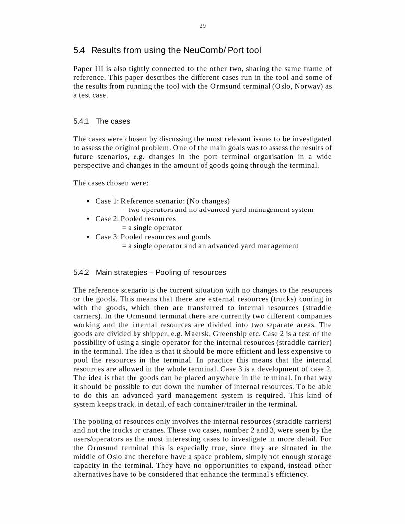
5.4 Results from using the NeuComb/Port tool Paper III is also tightly connected to the other two, sharing the same frame of reference. This paper describes the different cases run in the tool and some of the results from running the tool with the Ormsund terminal (Oslo, Norway) as a test case. 5.4.1 The cases The cases were chosen by discussing the most relevant issues to be investigated to assess the original problem. One of the main goals was to assess the results of future scenarios, e.g. changes in the port terminal organisation in a wide perspective and changes in the amount of goods going through the terminal. The cases chosen were:

•

Case 1: Reference scenario: (No changes) = two operators and no advanced yard management system

• Case 2: Pooled resources = a single operator

•

Case 3: Pooled resources and goods = a single operator and an advanced yard management

5.4.2 Main strategies – Pooling of resources The reference scenario is the current situation with no changes to the resources or the goods. This means that there are external resources (trucks) coming in with the goods, which then are transferred to internal resources (straddle carriers). In the Ormsund terminal there are currently two different companies working and the internal resources are divided into two separate areas. The goods are divided by shipper, e.g. Maersk, Greenship etc. Case 2 is a test of the possibility of using a single operator for the internal resources (straddle carrier) in the terminal. The idea is that it should be more efficient and less expensive to pool the resources in the terminal. In practice this means that the internal resources are allowed in the whole terminal. Case 3 is a development of case 2. The idea is that the goods can be placed anywhere in the terminal. In that way it should be possible to cut down the number of internal resources. To be able to do this an advanced yard management system is required. This kind of system keeps track, in detail, of each container/trailer in the terminal. The pooling of resources only involves the internal resources (straddle carriers) and not the trucks or cranes. These two cases, number 2 and 3, were seen by the users/operators as the most interesting cases to investigate in more detail. For the Ormsund terminal this is especially true, since they are situated in the middle of Oslo and therefore have a space problem, simply not enough storage capacity in the terminal. They have no opportunities to expand, instead other alternatives have to be considered that enhance the terminal’s efficiency.

30

5.4.3 Definition of efficiency This section is included to explain how the efficiency for the resources is defined in the tool. Efficiency as a measure is very hard to define in an exact meaning, but in this tool the efficiency of the resources is defined as:

t

ttteff T

QNLR ++=

effR is the occupied time divided by the total time. tL is the time in link, tN is

the time in node and tQ is the time in queue, all counted when the resource is occupied with cargo. All the resources have the same measure. It could be argued that other measures can be used and that different measure should be used for different resources, but this was the measure chosen. 5.4.4 Results Included here are two of the diagrams and the discussions about the results shown in Paper III to give the essence of the results from the use of the tool. The model/tool as such is a tactical/strategic tool that can be used for long term reorganisation issues in the port terminal. There are two ways of using the tool. The first is to use it as an optimisation tool for an already existing port terminal. The second is to use it as a simulation tool, where it is possible to simulate any given set of parameters in the port terminal. Figure 17 gives the efficiency figures for the current situation as described in section 5.4.1, the efficiency figures calculated as described in section 5.4.3 above. Figure 18 corresponds in its construction to Figure 17. The reason for including also figures without queues was that the users regarded it as useful to see the difference.

Current situation - Efficiency

100 100100,0 100,086,2

96,2

0

20

40

60

80

100

120

Efficiency with queues Efficiency withoutqueues

ReferencePooled resourcesPooled resources & cargo

Figure 17 Efficiency figures for the current scenario

31

The figures are indexed and related to the reference case (business as usual) terminal efficiency, which has been given the index of 100. The reason for this marginal cost reasoning is that if the basic figures for the cases, throughput volume, available resources etc. are the same, the system deviation will be marginal if only the changes are compared. This is a way of compensating for the eventual systematic deviations caused by errors in the figures used for building the models.

Future scenario - Efficiency

100 100

118,9

100,0

118,9111,4

0

20

40

60

80

100

120

140

Efficiency with queues Efficiency withoutqueues

Reference

Pooled resources

Pooled resources &cargo

Figure 18 Efficiency figures for the future scenario

When analysing the results some general remarks can be done. For the in-depth discussion is referred to Paper III. In the current situation where the throughput is fairly low, there is almost no difference between the cases except that there are substantially more queues in case 3, the pooled resources and cargo case. This is not intuitively clear. The reason is that when the cargo is pooled the tool will use the basic strategy that is a first come first serve basis. This means that the cargo chose the shortest path and therefor queues will be created. The small difference in efficiency without queues is due to more transhipments of the cargo. For the future scenario, with a much larger throughput, there are queues in all the cases. Here the highest efficiency is reached in the pooled resources case, which is expected since the queues and resource utilisation, is more evenly spread in a basically overloaded system. The pooled resources case gives less efficiency and considerable more queues. The reason is the same that was explained above. The interesting thing is that the efficiency without queues is almost the same. The explanation is that the cargo is more evenly spread in this case, and therefore the internal resources can be utilised better when pooled. The current situation is a sparse system that does not possess any large potentials for optimisation. For an elaboration of the issue see 5.5 below. The future scenario on the other hand is a much more dense system why the effect of an optimisations is larger.

32

5.5 Optimisation criteria and freedom of choice This part describes how the model is optimising the port terminal and what features/functions it is optimising. The reason for including this part is to create a base for understanding the choices that have to be made during the development of this kind of tool. The optimisation is divided into two parts: First there is one algorithm seeking out the maximum possible physical flow through the terminal. Secondly there is an algorithm optimising the resource utilisation on the boundary condition that the resources should interfere as little as possible with the principle of maintaining the maximum flow. This is a so-called optimal assignment problem. The problem to solve is that of performing a number of missions with a limited set of resources. After going through these two phases of optimisation the result is an optimal use of the available resources in the system. As mentioned above these optimisations are done according to the boundary conditions determined by the actual situation in the port terminal. A very crucial point when working with optimisation models, in contrast to simulation, is that there has to be certain numbers of degrees of freedom. This means that if everything is set to a specific value in the model, there will be no optimisation potential. This might be the reason why these kinds of models/tools are perceived as somewhat hard to follow, since it makes them less specific and more general. A large part of the work for this thesis has been dedicated to gather enough information to be able to understand what kind of decision rules are the most important to implement in this type of tool. Another consequence of this is that there have to be approximations about each port terminal and the functions within it. The result is that all the access control functions, corresponding to the gate, are considered equivalent, i.e. it is inessential, through which gate the goods pass. This is applicable to all the functions in the model/tool. It will of course always be possible to specify the model more, but then it will also be fewer possibilities to optimise the port terminal.

33

6 CONCLUSIONS & FUTURE RESEARCH This chapter gives the conclusions divided into two parts, the first about using the network approach as a base for assessing this kind of problem and the second one about the model and tool assessing the outcome of the project. The chapter ends with a short discussion about future research. 6.1 Network as a metaphor This way of describing a port terminal is seen as very useful, and actually any terminal or enterprise functioning in a similar way can be described. It has been presented within the EUROBORDER project and at several conferences and seminars and been positively received by both users in port terminals and academics. The model has been used to describe 6 different ports within this project. By using the network approach, that is a very common metaphor in the society (Casti, 1995), the port terminal model used in the project and in this thesis is easy to understand and use as base for discussions. Yet it is very useful from a pure modelling view, as in programming where it has been used in this project. The network approach allows us to break down the model from the aggregated level all the way down to the parameter level. This makes it very transparent and it is easy to choose the level of abstraction or detail needed. The model is flow oriented which makes it close to reality. 6.2 The model The results from working with the model and ultimately the tool is somewhat divided. On one hand some very interesting results have been extracted from runs with the tool, and it is clear that this approach is valid as abase for developing tools like this. It is also clear that it is a very useful way of assessing these kinds of problems. Port terminals, or e.g. any infrastructure dependent entity (which practically means all transport related activities) with large fixed costs and high barriers to change in the sense of capital investments can in an easy and cost efficient way evaluate different scenarios. On the other hand it is (and has been) a limitation to work with models and tools that are dependent on a quantitative approach. There exists a quite extensive research on optimisation and simulation, but few if any can handle a pure dynamic situation and none as far as the author is aware of can handle qualitative aspects. Despite the developments of both mathematical and computer science it is still hard to find a way to create a tool to assess the issue of the full complexity of an organisation that is dynamically changing. This was

34

one of the reasons why cybernetics was investigated, since it is a science that deals with automatic control and the notion of the black box theory. There are, in the author’s opinion a lot more to do in the field of optimisation as opposed to simulation, for instance incorporating qualitative aspects. There exist today a lot of good and well working simulation systems, e.g. Arena, etc. that can handle almost any type of systems in an acceptable way. The development here is only a difference in degree. In optimisation the situation is a bit different. There exist few, if any, really good working optimisation tools on the market today. The reason for this being the problem of incorporating the dynamic features of almost any system that is viable. Here a waste area of research is open, where knowledge from logistics, network theory and mathematics as well as computer science has to be incorporated. The conclusion can be summarised by stating that the value of the network approach and tools for assessing complex problems is confirmed to a certain degree. The project and thesis though also confirms that there is still quite a long way to go before we can handle truly dynamic systems. 6.3 Results The results can be divided in two parts, the first and most obvious results are those from the project and then primarily the use of the NeuComb/Port tool. The other part is coupled to the purpose and scope of this Thesis. The more tangible results from the use of the tool have been described in section 5.4 above and in Paper III. These results are not very detailed and deep, but what was shown was that this tool is suitable for pointing out areas suitable for changes and also to show these changes in a more general sense. It is also possible to show tendencies as answers to both theoretical and practical problems. An explanation may be in its place. It is of course possible to get answers like: The resource efficiency is 12,76% better, but due to rough input data and the constraints of quantitative tools, this is only a tendency that the system tested is better than the original one. The actual figure stated is false in its numeric value. This is also one of the major setbacks of quantitative tools like the one developed. It is necessary to develop these kinds of tools so that both qualitative and quantitative aspects can be incorporated in future models and tools. The NeuComb/Port tool is at least a first good step towards these kind of new tools made possible by advances in both Mathematical and Computer science.

35

The overall research question and the three more detailed questions are repeated below. Is it possible to enhance terminal efficiency without large capital investments?

• Can a port by modelling be treated like a generic terminal? • What tools is needed to expand the flow in existing ports? • What limitations exist for this expansion and are there an upper limit?

The answer to the overall research question is yes it is possible but it is hard to say how much, and it is highly dependent on which kind of terminal it is. As a general statement it is possible to say that the effect of changes in organisation, resource allocation etc. are better in more dense systems than better in more dense than sparse systems. This unfortunately corresponds to the effects of capital investments, it is a combination of economies of scale and scope, which also have an effect on more unorthodox methods. There is most probably an optimum between sparse and dense systems defining when those kind of enhancements have most effect, but that optimum has not been able to assess in this thesis. The project and Paper I-III describes the port as a terminal and it was used as a base for the port terminal model as well as the tool. It was seen as a very useful metaphor to describe both the structures in the port as well as the qualitative aspects. The terminal approach also made it possible to divide the port in separate areas that could be modelled together. The question about tools was actually aimed at the possibilities to enhance port terminal efficiency and as a consequence their throughput. It is an essential question since most ports are currently the bottleneck in the intermodal chain. One very simple answer to this is that the ship-to-shore cranes are the bottleneck in most cases. They decide the overall throughput for the port terminal, since the interface between the ship and the port is the crucial one of the simple reason that it takes up the most time. Other tools are of course terminal layout planning, advanced operative tools for allocation of resources in the terminals. The small and medium sized port against should take a benchmark process and best practice approach. The Southeast Asian ports have already implemented a lot of these kinds of systems and tools with Singapore as the leader. It is also possible to transfer knowledge from other areas as production simulation and optimisation in among others the car manufacturing industry. Other interesting industries are the aviation and railway industries tools for resource allocation, especially the crew scheduling models. The last question is actually quite easy to both assess and answer. Yes there is an optimum and it depends on the physical infrastructure and the resources available. This optimum can be calculated quite easily with the NeuComb/tool. It is called the theoretical optimum. The economical optimum is though a completely different thing. It is a well known fact that when the optimum is approached the cost groves exponentially.

36

6.4 Future research - Complex dynamic logistics systems During these years of my research I have become more and more aware of the effects the dynamic dimension of systems has on the complexity they possess. It is therefore not very hard to define my future research, which has actually already begun with an article written together with two of my senior colleagues at the department (Lumsden et al, 1998). This thesis can be seen as a specific case of what is to be the future research for me; complex dynamic systems. While working on this thesis and the papers constituting it, I became aware of the surprisingly complex structures and interactions that these kinds of systems contain. Therefore my intention is to develop these thoughts by concentrate upon complex dynamic systems trying to apply the knowledge from other research fields, e.g. Systems science, Cybernetics, Network Theory and Automatic control to Logistic systems. Especially cybernetics is seen as a promising field. The initiated reader can object that this is an old science that has not solved the problem either. This is true so far, but since cybernetics was born and developed the computer and mathematical sciences have made great progresses, which gives us the possibility to further research the possibilities of assessing that kind of very hard questions. It is though not very probable that it will be possible to include all the qualitative aspects necessary to correctly describe and control highly complex systems, but perhaps it is possible to get closer and closer in course of time. To be a bit more explicit the future research will be focused on assessing the problem of the increasingly complex systems and solutions that exist within the transport and logistics field. With a worldwide consolidation going on and more and more companies merging into larger corporations this field of research will be highly interesting. The research will be based on the concept of complexity applied to the transport and logistics context. Especially interesting to study is the possibilities of information systems and the possibility of using them to either make the systems less complex or as a possibility to actually handle the full complexity of real world systems. It is in today’s science seen as the very edge of science to study the effects of advanced information systems and their impact on decisions, profitability etc.4. A lot has been written about complexity and there are already definitions of complexity in other fields as for example very exact definitions in mathematics and Ashby’s definition belonging to systems science and cybernetics (Ashby, 1956). This research will be the base

4 To give some perspective on the concept of the value of information, especially information that can be given in advance, a short story told by Aristotle is cited (Aristotle, 1993). There was a man called Thales from Miletos who was known to be very sage, but living his life in peace and not much wealth to his name. When people asked him why he as being so wise was so poor, he answered that wealth was not his ultimate goal. However he decided to give them an example, and since he knew a lot about the nature and the weather he could in the winter see that it would be a rich harvest of olives that year. He then signed up all available capacity for pressing the olives in the valley where he lived. When the autumn came he rented them for twice the sum he had hired them for. An ancient example of the value of information.

37

for developing the concept for the transport and logistics case, including network theory and qualitative aspects.

INTERFACES (Node-Link)

DECOMPOSITION INTEGRATION

SIMPLICITY COMPLEXITY

SURPLUS CAPACITY SURPLUS TRANSPORT VERTICALINFORMATION

HORIZONTALINFORMATION

STRATEGY

SYSTEM

CONSEQUENCES

Figure 19 Complex dynamic logistics systems (Adapted from Lumsden et al, 1998)

To give a context to the future area of research, Figure 19 has been included. It describes 3 different levels of the logistics system (the original figure consists of 4 different levels, but the lowest level tools has been cut out since it does not refer to the same “tools” as referred to in this thesis). The highest level is the strategy level, where the basic decision is whether to choose disintegration or an integration strategy. The traditional approach has been to choose the disintegration strategy, which gives the next level, a simple system. We have not had knowledge or tools to handle the problems arising in complex systems why this strategy is the predominating in the transport industry today. The lowest level is the systems level showing the two dominating ways of creating simple enough systems to handle a complex demand or environment, surplus capacity or surplus transport e.g. frequency. The right hand side describes the other choice, which considers the area of interest for future research, complex solutions to match the complex problem. This is in line with Ashby’s Law of Requisite Variety mentioned earlier. This is currently handle by a combination of horizontal and vertical information and the extensive use of information systems. There is though very little research done about the reasons for transport systems being so complex and hard to handle efficiently. Most people conceive transport and logistics as something basically very simple, which is true on the basic level of getting a package from A to B, but as soon as the system grows and the connectivity in the network expands it soon gets out of our hands. 5 The main issue with future research must be to try to explain the underlying reasons and to define complexity in the transport and logistics context. 5 To prove my point I want the reader to consider the Box mentioned by Bowman (Here cited from Beer, 1959) The box has only 8 inputs and 1 output: a sufficiently simple system or machine as it is referred to in the original text. Adopting the constraint that the input and output can only take on one of only two values, (compare with binary states in today’s computers) how many possible machines can the Box represent? There are 82 input states. Now with an output of two possible states, the number of possible machines which the Box can simulate is n2 , where n is the number of distinguishable input states. So the number of

distinguishable states are 822 or 2562 ! Just how large a number this is becomes fully apparent

when it is compared with Eddington’s Cosmical Number; for according to Eddington, the total number of protons and electrons in the universe is 3/2.136. 2562 . Thus so simple-looking a Box has sufficient variety in its distinct manifest to parallel the variety of the universe (Beer, 1959).

38

The research will be divided into three stages most probably resulting in three papers. Firstly there will be a theoretical assessment of how complexity in transport and logistics systems can be described, aiming at a first attempt to give a “working” definition of complexity applied to the area of transportation and logistics. Secondly, a case study on a large enough system will be performed to test the ideas and concepts developed in the first phase. Finally the results will be analysed and a second refined assessment of the concept of complexity in dynamic logistics systems will be done.

39

7 REFERENCES Arbnor, I. and Bjerke, B. (1997). Methodology for Creating Business

Knowledge (2nd ed.), Sage Publications, Thousand Oaks, USA Aristotle (1993) Politiken, (Blomqvist, K. Ed.) Paul Åströms förlag, Jonsered,

Sverige Ashby, R.W. (1956) An Introduction to Cybernetics, Chapman & Hall Ltd,

London, Great Britain Beer, S (1959) Cybernetics and Management, The English universities press Ltd,

London Great Britain Beer, S (1985) Diagnosing the System for organisations, The Managerial

Cybernetics of Organisation, John Wiley & Sons von Bertalanffy, L. (1968) General Systems Theory, George Braziller, New

York, USA Bowman, J.R. (1953). Reduction of the Number of Possible Boolean Functions,

Transactions of Ninth American Conference on Cybernetics, Josiah Macy Jr. Foundation, New York, USA

Carlsson, Jan-Olof (1999), Agile Distribution and a Dynamic Coupled Logistical

Systems Approach. Working Paper, Breakpoint Consulting, Göteborg, Sweden.

Casti, J. (1995). The Theory of Networks. In: Networks in Action , (Batten D.

Casti J. and Thord R. Ed.) Springer-Verlag, Berlin, Germany Checkland, P.B. (1981). Systems Thinking – Systems Practice, John Wiley &

Sons, Chichester, USA Churchman W.C. (1981). The Systems Approach. Dell Publishing Co. Inc., New York, USA Crainic, T.G., Dejax, P. and Delorme, L. (1989). Models for Multimode

Multicommodity Location Problems with Interdepot Balancing Requirements, Annals of Operations Research, 18 , pp. 279-302.

ECMT (1993) Terminology on Combined Transport, OECD, Publications

Services, Paris, France European Commission Green paper on Ports, (1998). European Union,

Brussels, Belgium EUROBORDER D3.1. (1997) TFK Hamburg, Germany

40

EUROBORDER D5. (1998a). TFK Hamburg, Germany EUROBORDER Program manual. (1998b). TFK Hamburg, Germany EUROBORDER internal validation report. (1998d). CECIL, Göteborg,

Sweden Frankel E.G. (1987). Port Planning and Development. John Wiley & Sons, New

York, USA Hellevik, O. (1977). Forskningsmetoder i sociologi och statsvetenskap, Natur &

Kultur, Lund, Sweden Hulthén, L.A.R.(1997). Container logistics and its management, Report 32,

Department of Transportation and Logistics, Chalmers University of Technology, Göteborg, Sweden

Håkansson, H. (1989) Corporate Technological Behaviour – Co-operation and

Networks, Routhledge, London, Great Britain Jansen, K. (1998). Background of a tool for optimising resources on a

transportation network, Mathematics in Transport Planning and Control, (Griffiths, J. D. Ed.) - Proceedings of the 3rd IMA International Conference on Mathematics on Transport Planning and Control, pp 187-195, Pergamon, 1998, Great Britain

Jungnickel, D. (1994). Graphen, Netzwerke und Algorithmen, BI

Wissenschaftsverlag, Berlin, Germany Kalman R.E and DeClaris N. (1971). Aspects of Network and System Theory.

Holt, Rinehart and Winston, Inc., New York, USA Kondratowicz, L.J. (1990). Simulation methodology for intermodal freight

transportation terminal. Simulation, July, pp. 49-57 Kondratowicz, L.J. (1993). MULTIMOD – The system for simulation modelling

of seaports and terminals as logistics centres in intermodal freight transport / Simulation in logistics planning, Publications from the center for maritime studies, University of Turku, Turku, Finland.

Kuhn, T.S. (1970) The structure of scientific revolutions (2nd ed.), The University

of Chicago Press, Chicago, USA Lumsden, K.R. (1995). Transportekonomi – Logistiska modeller för

resursflöden, Studentlitteratur, Lund, Sweden Lumsden, K.R. (1998). Logistikens grunder, teknisk logistik, Studentlitteratur,

Lund, Sweden

41

Lumsden, K.R. (1999), Logistics complexity in mobility systems, Working paper, Department of Transportation and logistics, Chalmers University of Technology, Göteborg Sweden. Lumsden, K.R., Hulthén, L.A.R., Waidringer, J. (1998). Outline for a

Conceptual Framework on Complexity in Logistic Systems, Opening markets for Logistics, (Bask, A.H. and Vespäläinen, A.P.J. Ed.) Proceedings of the Annual Conference for Nordic Researchers in Logistics – 10th NOFOMA 98, Finnish Association of Logistics, Helsinki, Finland

Magnanti T.L. and Wong T.R. (1984). Network Design and Transportation

Planning: Models and Algorithms. Transportation Science, 18, pp. 55 Manheim M.L. (1984). Fundamentals of Transportation Systems Analysis;

Volume 1: Basic Concepts, The MIT Press, Cambridge, USA Ojala L. (1992). Modelling approaches in port planning and analysis,

Publications of the Turkuu school of economics and business administration, Series A-4:1992, Turkuu, Finland

Sjöstedt, L (1999). Unpublished lecture notes, Department of Transportation and logistics, Chalmers University of Technology, Göteborg Sweden Waidringer J. & Lumsden K. (1997). Modelling a Port terminal from a Network

perspective, Proceedings of the 13th International Conference on Automatic Control, Chania, Greece.

Waidringer, J. & Lumsden, K. (1998). Simulation and optimisation of Port terminals, using a network concept, presented, 8th World Conference on Transport Research, Antwerp, Belgium, Wagner, H.M (1975). Principles of Operations Research, with applications to

managerial decisions, (2nd ed.) Prentice Hall, Englewoods Cliffs, New Jersey, USA

Wandel, S. & Ruijgrok, C. (1995) Information Technologies for the

Development of Transport and logistics; A Systems Model and Examples, ATAS Bulletin Information Technology for Development, United Nations, New York, USA.

Wiener, N. (1948) CYBERNETICS or control and communication in the animal

and the machine, The M.I.T. press and John Wiley & Sons, New York, USA Woxenius.(1998). Development of small-scale intermodal freight transportation

in a systems context, Report 34, Department of Transportation and Logistics, Chalmers University of Technology, Göteborg, Sweden

APPENDIX I Modelling a port terminal from a network perspective

Waidringer, J. & Lumsden, K.R. Presented at the 13th International Conference on Automatic Control, Chania, Greece, June 16-18 1997. Published in proceedings.

1

MODELLING A PORT TERMINAL FROM A NETWORK PERSPECTIVE

Jonas Waidringer*, **, M.Sc. & Kenth Lumsden*, PhD.

* Department of Transportation and Logistics, Chalmers University of Technology, 412 96 Göteborg, Sweden

** Center at Eriksberg for Communication, Information and Logistics,

Blå Hallen, Eriksberg, 417 64 Göteborg, Sweden Abstract: This paper gives an efficient way of describing a Port terminal at a micro level, where it uses two foliated networks, an information flow network and a cargo flow network. The model works with nodes and links that both are characterised by a set of parameters, the real characteristics of a Port terminal as a base for mathematical functions. There is a strong need for theoretical, and practical, tools to simulate and optimise the operations in a Port terminal. The ports are today an important link, which gives great value to knew ideas how to change the port operations. The model is tested against port operators and scientist within an EU research project. Keywords: Network theory, Simulation, Optimisation, Port terminals

1 INTRODUCTION The ports are an important but week link in the transport chain, which gives great value to knew ideas how it is possible to change the port operations (Frankel, 1987). Currently there exist few, if any, models describing the Port terminal from a pure network perspective (Ojala 1992, and references therein). This paper derives from the need for a model of a Port terminal, described out of a network concept. The model is used in an EU research project; EUROBORDER. In this project an optimisation tool will be built that works with two foliated networks; an information flow network, a cargo flow network and a set of resources constituting these networks. This relates closely to a conceptual framework developed for resources (Manheim, 1979). The core of the model is the cargo flow and the corresponding network, since this is seen as the Port terminal’s main function, and the essence of its activities. This generic model of a Port terminal has also an academic interest since it is a different and structured way of describing the interrelations within the Port terminal system.

2

2 FRAME OF REFERENCE: THE PORT The port environment is described first to define the port as a part of an overall transport chain.

Industrial system

Market system

Port system

Transport system

Political system

Supplier system

SupplyDemand

RegulationStimulation

ProductsServices

Services

Demand ProductsServices

RegulationStimulation

RegulationStimulation

Fig. 1: The environment of the port (Hulthén and IAHP, 1996) How the environment influences the port system can be described with activity relations (figure 1). No detailed description about the port system and how the environment and the port system interacts will be done. Instead this should be seen as a way of defining the reference system for this paper. Port models used as a base for planning and analysis may be classified in the following way (Ojala, 1992 and references therein): • Models with an econometric approach • Models with an analytic approach • Models using simulation technique Econometric models deals normally with the macro-level aspects, and are widely used in research problems related to demand and supply. A system is described as a casual network of relationships between a set of variables. Analytic models are created within the framework of Operations Research (OR). The basic idea is to develop a mathematical function which can be solved by an algorithm under certain constraints. Simulation models use a numerical technique for specific mathematical models to analyse time-bound flows of events within a system, consisting of a large number of variables and constraints. To give a background to our model some examples of how to describe a Port terminal is given, beginning with the Port terminal as a "black box" , as shown in figure 2.

3

PORTTERMINAL

CARGOTYPE 1 IN

CARGOTYPE 2 IN

CARGOTYPE 1 OUT

CARGOTYPE 2 OUT

INFORMATIONIN/OUT

RESOURCESIN/OUT

Fig. 2. Different flows through the Port terminal The description above is the simplest possible way of describing a Port terminal, in terms of logistical flows. The Port terminal is seen as a "black box" with cargo, information and resources going in and out of the box. What happens with the different flows is not taken into account, instead focus is on the results, i.e. what is actually going in and out of the model. This is in line with the systems approach (Churchman, 1981): “The way to describe an automobile is first by thinking about what it is for, about its function, and not the list of items that make up its structure” Within this frame the Port terminal is described with 3 main functions, receive/delivery, load/unload and transfer as shown in figure 3 below.

L o a d /U n lo a d

R e c e iv e /D e liv e ry

T ra n s fe r

L a n d s id e P o rt te rm in a l S e a s id e

Fig. 3: The Port terminal described by its functions The analytical approach described above is used as a frame of reference for this paper, since the model developed is created as a base and as a tool for simulation and optimisation.

4

3 NETWORK THEORY Network theory is used in this paper as a base for describing a Port terminal and to build the model. In this chapter the ideas and theory of networks coupled to the frame of reference is given. A network can be defined as nothing more (or less) than a system (Casti, 1995). network objects connections system= + = Such a network can mathematically be described as a graph. A graph is simply a set of nodes V together with a set of edges E . The most important feature of a network is the connectivity, i.e. if the nodes and edges are connected through the network, and permits interactions (Casti, 1995). This paper only discusses graphs and networks that are connected. This relates to the fact that the Port terminal is related to as a system, and this system has to correlate, to work properly. The different topics captured by the network model are another way of describing it (Magnanti and Wong, 1984). “Indeed, network design issues pervade the full hierarchy of strategic, tactical and operational decision-making situations that arise in transportation.” The network design is very important for the actual model, and what it is supposed to be modelling. Our model serves as a base for both a vehicle routing problem, i.e. how the flow is going through the network, and a facility location problem, i.e. the network lay-out. Another crucial point in the model is based on Neural Networks and Combinatorial Graph theory. There are possible interactions in both the links and the nodes. A combination of the two most common ways of describing a network is done. Either as a network of nodes connected by links, where only the nodes are characterised by parameters, or with the nodes only expressing the topology of the network and all other characteristics are associated with the links.

R/D

R/D

T T

T T

T S S L/U

I1 I2 R1

CargoType 1 IN

CargoType 1 IN

=Cargo node =Information node

=Resource node

CargoType 1 OUT

CargoType 2 OUT

Fig 4. The Port terminal as a combination of different nodes and links

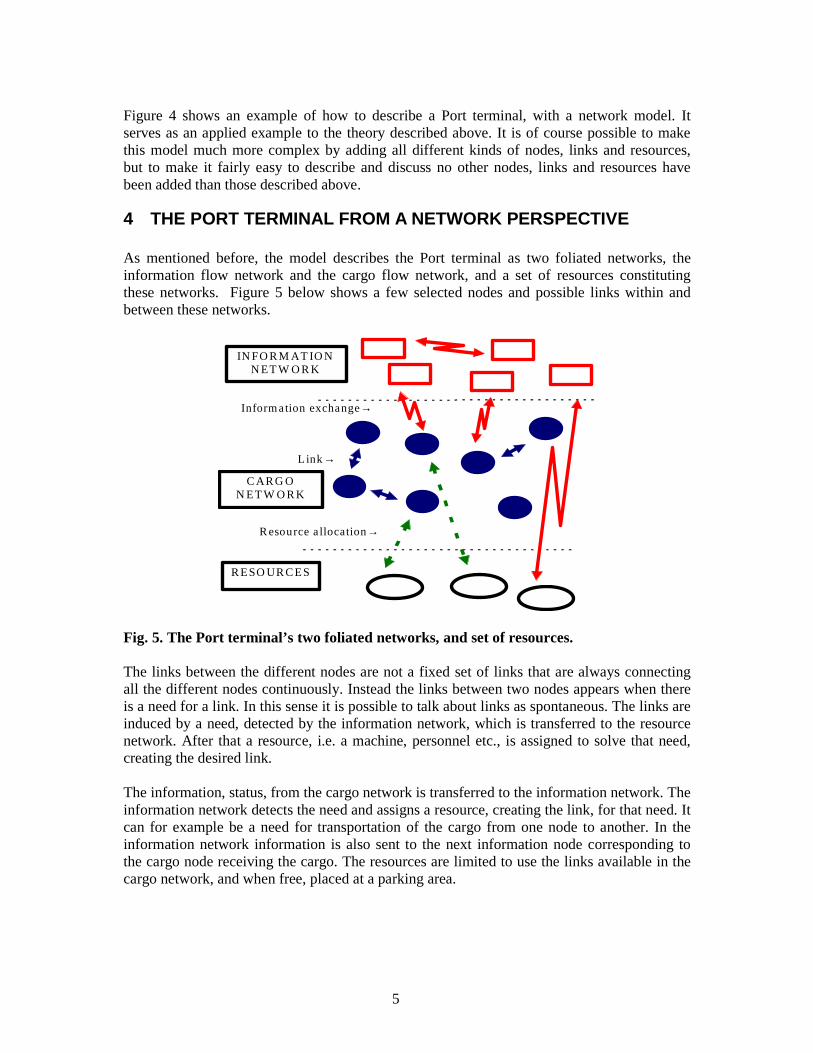
5

Figure 4 shows an example of how to describe a Port terminal, with a network model. It serves as an applied example to the theory described above. It is of course possible to make this model much more complex by adding all different kinds of nodes, links and resources, but to make it fairly easy to describe and discuss no other nodes, links and resources have been added than those described above.

4 THE PORT TERMINAL FROM A NETWORK PERSPECTIVE As mentioned before, the model describes the Port terminal as two foliated networks, the information flow network and the cargo flow network, and a set of resources constituting these networks. Figure 5 below shows a few selected nodes and possible links within and between these networks.

IN FO R M AT IO NN ET W O R K

C AR G ON ET W O R K

R ESO UR C ES

R esource a llocation→

Inform ation exchange→

Link→

Fig. 5. The Port terminal’s two foliated networks, and set of resources. The links between the different nodes are not a fixed set of links that are always connecting all the different nodes continuously. Instead the links between two nodes appears when there is a need for a link. In this sense it is possible to talk about links as spontaneous. The links are induced by a need, detected by the information network, which is transferred to the resource network. After that a resource, i.e. a machine, personnel etc., is assigned to solve that need, creating the desired link. The information, status, from the cargo network is transferred to the information network. The information network detects the need and assigns a resource, creating the link, for that need. It can for example be a need for transportation of the cargo from one node to another. In the information network information is also sent to the next information node corresponding to the cargo node receiving the cargo. The resources are limited to use the links available in the cargo network, and when free, placed at a parking area.

6

Realisable links

Desired links

Realised links

Fig. 6. Different sets of links Figure 6 above explains the way different types of links used in this modelling process are defined. The realisable links are all links between all nodes in the network, that are realisable defined by some kind of criteria such as cost etc. Desired links are links one would like to use if there were no constraints on the network. Realised (physical) links are the links finally realised, by the set of resources, when all constraints have been imposed to the network. The total set of links in the network, called abstract (AL) or theoretical links, are the union of the realisable (RL) and desired (DL) links. AL RL DL= � Cargo flow network - Cargo nodes The type of node is defined by the network it belongs to. A cargo node is therefore a node belonging to the cargo network. 4 different types of nodes describe the cargo network, in line with the reference model described in chapter 2 and related to the four terminal functions described by Chadwin et al. (1990) Receive/Delivery (Land side), this is the Port terminal’s interface with the land side, i.e. road and rail. This node contains functions like id-control, physical entrance etc. Load/Unload (Sea side), this is the Port terminal’s interface with the seaside, i.e. all waterborne transport. This node is the mirror node to the receive/delivery node. Due to the difference in functions between these two, there are different nodes. Transfer, this is where all the transfer between different transport modes is taking place. On an aggregated level it is the essence of a Port terminal, the transfer between land based and sea based transportation modes. Storage, this is where the cargo is stored in between the different transportation modes. A more correct name would be “waiting” node, since the cargo does not necessary has to be stored in the common sense. Instead the cargo has to be accumulated in the Port terminal because of the difference in size between the cargo carriers, which creates a necessary waiting time. Information flow network - Information nodes There are also a number of information nodes, but only two different types are needed in this network model.

7

External system information node, which causes constraints on the cargo flow. This information comes from outside the system modelled, outside the Port terminal. For example all the documents needed for customs clearance are, if they are not available causing a constraint on the cargo flow. Internal system information node, which supports the cargo flow and allows us to optimise. This information is generated within the system. For example information about a storage area being full, gives us the opportunity to redirect the cargo flow. A note on external and internal information on a given network external information can not give a faster throughput, but internal information can. The external information is though capable of changing the whole network. Set of resources - Resource nodes The third and last kind of node is the resource node, and it is sufficient with one kind. This node contains a resource, for example machines, personnel etc., which can be used to handle the cargo and/or information flow. All these different nodes are in the next level divided into several subnodes, that together give the full description of the node. The nodes can also be described with parameters as described in figure 7 below.

A B C D E

I1 I2

IN OUT

F

R

Node border Fig. 7. A node described as a combination of parameters Our model is based on an analytical model approach, and it is hence necessary to be able to quantify the functions. This is done by describing the node, links and resources with parameters. Figure 7 above shows the parameters for a node that belongs to the cargo flow network. It is a convenient and sufficient way to describe a node. The parameters describe the flow through the node, whether it is cargo or information. For example; the speed parameter describes the speed of the flow through the node. The parameters are: A. Cargo type Ct], dangerous, reefer etc. B. Time [t] C. Length [s], length of the transportation of the cargo within the node D. Speed [v], the speed which the cargo moves through the node E. Cost [c], the cost of handling the cargo in the node F. Transformation [St - St’], the status of the cargo, i.e. entered, finished etc.

8

The function describing the node is realised by the parameters given above: f f A B C D E F= ( , , , , , )

It is possible to use more parameters, but since this is only an introduction to this idea of describing a node there are no more parameters added than those described. The information and resource nodes correspond to the cargo nodes described above, and are in the same way described by similar parameters. In this model the nodes are described and defined in the following way: • Type of node, defined by which network it belongs to, i.e. the cargo-, information or set of

resources. • The parameters constituting the node • Description of the node in words, and subnodes A link can be defined in a way similar to the definition of nodes. A link is defined by its type, parameters, a description, and by its start and end nodes. The definition of a link: • Type of link, defined by which network it belongs to • Parameters constituting the link • Description of the link in words • The start and the end nodes of the link The difference though, from the nodes, is that the links are dynamic, only appearing for short time periods when they are actually needed. There are no static connections in the form of links between the different nodes. The nodes however are static in the sense that even if there is no activity in the node it still exists, as are the resources. Hence the total network per se, does not exist the resources are assigned to establish the links and thereby constitute the network. This means that the cargo network can not exist without the information network and the set of resources, which creates the links in the cargo network. In a similar way, the information network does not exist without resources creating the links in it. The resources are of course different from the resources in the cargo network. These links are constituted by their parameters in the same way as described for the links above. There are also links between the information network and the two other networks as shown in figure 5 above. In the model the terms functions and subfunctions are used to describe the cargo network and the term process to describe the information network. Figure 8 below illustrates this.

9

Information flow

Cargo flow

Resources

Time

ActionProcess

Function

Fig. 8. Information processes and cargo functions, and the interaction between the

information processes, cargo functions and resources It also describes the interaction between the cargo flow, information flow and the resources. Both the information flow and the resources (availability) put constraints on the cargo flow. When the cargo flow reaches a node it stops. There is no cargo flow within the node, at the current level of abstraction, but a flow through it. When the cargo flow stops in the node, an information process is activated. When this process is finished, the cargo flow continues. If a resource is available at the time needed the transport assignment is performed, otherwise the cargo flow is stopped until a resource is available. The graph describing the cargo network above can be expressed mathematically in the following way:

( )G V E= , V = the set of nodes E ⊂ R 2 ,a set of links within the set of resources E is also defined by the information that is assigning the resource to the cargo network. (For further definitions and explanations, please see the appendix)

5 CONCLUSIONS In this paper the frame of reference; the Port terminal and the network theory has been described and finally these two were combined into a network model of a Port terminal. This way of describing a Port terminal is seen as very useful, and actually any terminal or enterprise functioning in a similar way can be described. It has been presented within the EUROBORDER project, and received positively by users in Port terminals, and those users are Port terminal planners and others that work with planning and organisation of ports. The model has been used to describe 6 different ports within this project. By using the network approach, that is a very common metaphor in the society (Casti, 1995) our Port terminal model is easy to understand and use as base for discussions. Yet it is very

10

useful from a pure modelling view, as in programming where it has been used in the EUROBORDER project. The network approach allows us to break down the model from the aggregated level all the way down to the parameter level. This makes it very transparent and it is easy to chose the level of abstraction or detail needed. The model is flow oriented which makes it close to reality. There remain things to do within this area, such as look deeper into the connections, and interactions between the networks and the set of resources. There is also still a need for a good description of a pure information network, and its possible utilisation as the management tool for networks.

6 REFERENCES Casti, J. (1995). The Theory of Networks. In: Networks in Action , (Batten D. Casti J. and

Thord R. Ed.) Springer-Verlag, Berlin Chadwin M.L. Pope J.A. Talley W.K. (1990). Ocean container transportation: an operations

perspective. Taylor & Francis, New York Churchman W.C. (1981). The Systems Approach. Dell Publishing Co. Inc., New York Frankel E.G. (1987). Port Planning and Development. John Wiley & Sons, New York IAHP. (1996). Future Role of Ports in Combined Transport (Hulthén. L. Ed.) IAHP Head

Office, Japan. Kalman R.E and DeClaris N. (1971). Aspects of Network and System Theory. Holt, Rinehart

and Winston, Inc., New York Magnanti T.L. and Wong T.R. (1984). Network Design and Transportation Planning: Models

and Algorithms. Transportation Science, 18, 1-55 Manheim M.L. (1984). Fundamentals of Transportation Systems Analysis; Volume 1: Basic

Concepts, The MIT Press, Cambridge Ojala L. (1992). Modelling approaches in port planning and analysis, Publications of the

Turkuu school of economics and business administration, Series A-4:1992, Turkuu

11

A. MATHEMATICAL DEFINITIONS Networks, and some related concepts (Based on Batten et al, 1995, Kalman and DeClaris, 1971 and Magnanti and Wong, 1981). Let G V E= ( , ) be a graph with V = a set of nodes and E = a set of links. At the same time a weight function is introduced, w E= → R on the graph, which to each link, e, attaches a weight ( )w e ∈ R . The couple ( )G w, is called a network.

( )w e could here be any relevant quantity for the link, e.g. time needed to traverse the link, its capacity, the cost for traversing the link, probability for success in trying to traverse the link etc. Let G be connected, i.e. for any pair of nodes there exist a walk (succession of links) connecting the nodes. For any path (i.e. a walk with all nodes and links different): P v v v ve e e

nn: ...0 1 2

1 2 → → → → , where e vi i denotes links and denotes nodes,

the weight is defined as c P w ei n i( ): ( )min= ≤ ≤1 As for nodes and link, they are of course mostly a consequence of our way of visualising graphs in two dimensions. Somewhat more formal, given any set of V elements of some kind ( e.g. points in R n ) and let E be a subset of V V× then by definition the pair ( , )V E is a graph with nodes being the elements in V and links being pairs of elements in V , i.e. e E∈ means

{ }e a b= , for some elements a b, in V . Drawing the graph ( , )V E , { }e a b= , is of course identified as the straight line, ”link”, between a and b.

Paper II Simulation and optimisation of port terminals using a network concept

Waidringer, J. & Lumsden, K.R. Presented at the 8th World Conference on Transport Research, Antwerp, Belgium, July 12-17, 1998. Considered for publication in the International Journal of Maritime Economics.

1

SIMULATION AND OPTIMISATION OF PORT TERMINALS, USING A NETWORK CONCEPT

Jonas Waidringer*, **, M.Sc. & Kenth Lumsden*, PhD.

* Department of Transportation and Logistics, Chalmers University of Technology, 412 96 Göteborg, Sweden

** Center at Eriksberg for Communication, Information and Logistics,

Blå Hallen, Eriksberg, 417 64 Göteborg, Sweden Abstract: This paper describes the theoretical basis for a newly develop tool, NeuComb/Port, as well as the actual tool itself. The basis for this tool is neural networks and combinatorial graph theory. In the paper some results from a set of runs on a real case, the Oslo port, are given. A short discussion about the implications of possible changes of a port terminal out of the results from an optimisation of the Port terminal is also given. The results are derived from a set of simulations and optimisations done in co-operation with a number of European ports, within the EU project, EUROBORDER

1. INTRODUCTION There exist a number of ways of describing a port, e.g. any terminal, but few from the network perspective. This paper addresses the issue of evaluating and choosing different parameters to describe the port out of a network perspective, and as a result proposes a model, NeuComb/Port. The need for this kind of description and model derives from the need to create a simulation and optimisation tool at a micro level. Since the network is a set of nodes and links, the parameters have to be consistent. The model, which is the result of this paper, is built on network theory in general and neural1 networks and combinatorial graph theory in specific. Another restriction is that the parameters have to be quantitative, since the network model is based on mathematical operations. The model as such is a tactical/strategic tool that can be used for long term reorganisation issues in a Port terminal, since the model is developed into a PC based optimisation and simulation tool. This means either to simulate physical reconstruction, with corresponding changes in the terminal flow, or reorganisation of the work in the Port terminal e.g. changes in the resource distribution. There are two ways of using the tool. The first is to use it as an optimisation tool for an already existing Port terminal. The second is to use it as a simulation tool, where it is possible to simulate any given set of parameters in a Port terminal. The simulation is also used as a way of validating the model. The cargo throughput and the resource utilisation are the main issues for optimisation, under the consideration of the constraints implied by the information, administration and legal factors. The networks are just a way of explaining abstract interactions and interrelations in the model.

1 The part of neural nets that is used in this paper is the possibility to have information in both nodes and links

2

The optimisations are done according to the boundary conditions determined by the information, organisation and legal conditions in the Port terminal. The model works with a superposition of three networks, which is though only a way of describing it graphically and in words. In the model/tool boundary conditions are used to be able to take information, organisation and legal constraints into consideration when optimising, as well as simulating the Port terminal. The NeuComb/Port tool makes it possible to build a model of any Port terminal with its specific characteristics. The result from the model is either an optimal use of the resources according to a given flow or an optimal flow according to a given set of resources. There is also a result from the simulation part that shows the flow and the resource utilisation according to the parameters set in the model. The result is displayed graphically as well as numerically. The tool is made with a generic2 Port terminal model as a demo and with default values on all the parameters involved.

2. FRAME OF REFERENCE In this chapter the port environment is described to define the port as a part of an overall transport chain. A short description of different possible models that can be used is also included, as well as the main parts of a Port terminal.

Industrial system

Market system

Port system

Transport system

Political system

Supplier system

SupplyDemand

RegulationStimulation

ProductsServices

Services

Demand ProductsServices

RegulationStimulation

RegulationStimulation

Figure 1 The environment of the port (Hulthén and IAHP, 1996) How the environment influences the port system can be described with activity relations as shown in figure 1. No detailed description about the port system and how the environment and the port system interact will be done. Instead this should be seen as a way of defining the reference system for this paper. Port models used as a base for planning and analysis may be classified in the following way (Ojala, 1992 and references therein): • Models with an econometric approach • Models with an analytic approach • Models using simulation technique

2 Generic is used in the sense of an aggregated, non-specific, model

3

Econometric models normally deal with the macro-level aspects, and are widely used in research problems related to demand and supply. A system is described as a casual network of relationships between a set of variables. Analytic models are created within the framework of Operations Research (OR). The basic idea is to develop a mathematical function, which can be solved by an algorithm under certain constraints. Simulation models use a numerical technique for specific mathematical models to analyse time-bound flows of events within a system, consisting of a large number of variables and constraints. To give a background to the model some examples of how to describe a Port terminal is given, beginning with the Port terminal as a "black box", as shown in figure 2 below.

PORTTERMINAL

CARGOTYPE 1 IN

CARGOTYPE 2 IN

CARGOTYPE 1 OUT

CARGOTYPE 2 OUT

INFORMATIONIN/OUT

RESOURCESIN/OUT

Figure 2 Different flows through the Port terminal The description above is the simplest possible way of describing a Port terminal, in terms of logistical flows. The Port terminal is seen as a "black box" with cargo, information and resources going in and out of the box. What happens with the different flows is not taken into account, instead focus is on the results, i.e. what is actually going in and out of the model. This is in line with the systems approach (Churchman, 1981): “The way to describe an automobile is first by thinking about what it is for, about its function, and not the list of items that make up its structure” Within this frame the Port terminal is described with 3 main functions, receive/deliver, transfer and load/unload as shown in figure 3 below.

4

Load /U n load

R eceive/D eliver

T ran sfer

Lan d sid e Port term in al S ea s id e

Figure 3 The Port terminal described by its functions The analytical approach described above is used as a frame of reference for this paper, since the model developed is created as a base and as a tool for simulation and optimisation.

3. THE MODEL The NeuComb/Port model is developed to support the analysis of how the efficiency of a Port terminal as a part of the transport chain can be improved and thereby improving the competitive position of shipping in relation to the other transport modes. The boundary for the model is the Port terminal since it would not be feasible to model a larger environment within a quantitative model as this. The complexity of the Port terminal is also enough to make it impossible to model without making approximations about the environment. The NeuComb/Port model has a pure research dimension to it, since it is the first model developed with the aim to give, in an absolute sense, an optimal solution to the flows through a Port terminal. Given here is a description of the NeuComb/Port model. The program is an implementation of strong mathematical algorithms adjusted to a port environment. The optimisation is divided into two parts: First there is one algorithm seeking out the maximum possible physical flow through the terminal. Secondly there is an algorithm optimising the resource utilisation under the boundary condition that the resources should interfere as little as possible with the principle of maintaining the maximum flow. This is a so-called optimal assignment problem. The problem to solve, is that of performing a number of missions with a limited set of resources. The result after going through these two phases of optimisation is an optimal use of the available resources in the system. As mentioned above these optimisations are done according to the boundary conditions determined by the information, organisation and legal conditions in the Port terminal. This is in line with what has been described in a paper about distribution planning of containers in the Port of Singapore (W.S. Shen & C.M. Khoong, 1995).

Figure 4 Flow scheme for the optimisation

Scanning the system

Free flow optimisation

Scanning the system

Optimal assignment

Resource allocation

5

A crucial point when working with optimisation models, in contrast to simulation, is that there has to be a certain degree of freedom. This means that if everything is set to a specific value in the model, there will be no optimisation potential. This might make users perceive the model/tool as somewhat rough to follow, since it makes it less specific and more general. A large part of the work with the model has been dedicated to gather enough information as a base for a decision about what is possible to optimise within a Port terminal. Another consequence of this is that there have to be approximations about each Port terminal and the functions within it. The result is for example that all the access control functions, corresponding to the gate, are considered equivalent, i.e. it is inessential, which gate the cargo passes through. This is applicable to all the functions in the model. It will of course always be possible to specify the model more, but then it will also be fewer possibilities to optimise the Port terminal. The model basically works as follows: • Simulation of the physical and information flows • Optimisation of the physical and information flows • Optimal matching of the resources under the boundary constraints The data input will be made in three steps: • “Static” configuration, i.e. the infrastructure of the Port terminal. All nodes and

links possible, with associated capacities, costs, times, types etc. • “Dynamic” configuration, i.e. all constraints, put on the static configuration, such

as boundary conditions associated with the information. Here will also the distributions of different flows be put in.

• “Operative” configuration, i.e. the specific conditions associated with the scenario that is going to be implemented. It can be cargo throughput, changes in resource allocation etc.

The parameters keyed into the static configuration will be more or less static parameters that are describing the specific port. In short, this phase is creating a model of that specific port. When this is done the model/tool will also be calibrated to that specific port, since the parameters keyed in is specific for that port and not the generic ones. This part is crucial, since the validity of the model/tool is directly depending on the accuracy of the parameters keyed in. If the values of these parameters are inaccurate then the model will be false. This is of course true for any model; no model is better than the quality of the numerical values of the appropriate parameters. Before describing the program more in detail the concepts of the model are described. The first thing to note is that the model only works with unit loads, secondly the port functions, have to be broken down into smaller elements in order to be able to simulate and optimise the Port terminal operations. In the model there are four elements which in different combinations constitute the port functions. These four elements, which describe the infrastructure of the physical flow, are action nodes, queue nodes, wait nodes and links. In the NeuComb/Port model nodes are instances where the cargo is not undergoing physical transition or instances where the cargo

6

change transportation mode. Links are connections between nodes. In a link the cargo undergoes physical transition. Information is added on to the system as boundary constraints. In an action node some kind of action, which takes a specified amount of time is carried out. There is only one kind of action node regardless of what the action is. In the model an action node only has place for one cargo unit at the same time. Queue and wait nodes have place for more than one cargo unit, and the time in the node depends on the following nodes and not on the node itself. In queue nodes cargo units are accessed based on first come first served basis, FIFO. In wait nodes any cargo unit can be accessed at all time. The links in the physical network are described by the same parameters as the nodes, i.e. capacity, time and cost for that specific link. The links in the information network are just connecting the information nodes and the physical nodes, since the capacity is regarded as unlimited, time very short and almost no costs. The nodes correspond to the actions performed in a port terminal, such as ID-control, gates, storage areas and so on. Each node in the model is represented by a combination of the model specific nodes to be able to describe it as exact as possible. For example, three model specific nodes describe a transfer node. First a queue node to handle the possibility of a queue in to the node. Then an action node where the actual handling is performed, and finally another queue node that makes it possible to handle the possibility of a queue out of the node, if there are no available resources at that time. For a complete description and names of these nodes, see (J. Waidringer & K. Lumsden, 1997) for further descriptions. To handle the constraints imposed by lack of information, other administrative and legal issues the information network is constructed as a delay function. Each node can be assigned a delay in form of an exponential distribution. The actual information delay is then randomly distributed within the limits given by the specific exponential distribution, determined by the maximum value and lambda value. The limits are decided and entered into the model in the initiation phase of the modelling. To give a concrete example; if a Port terminal in average experience a delay of about 5 minutes and a maximum delay of about 10 minutes in the gate function the user will enter the maximum value and a constant corresponding to the shape of the distribution. Then the model is randomly giving delays within these frames.

To be more exact the delay and distribution is done in the following way: The delay can vary between 0 and maxτ .

( )ξτττ fmax+=

Where τ is the time in the node, τ is the average time in the node without the information delay, maxτ is the maximum time delay imposed by the information and

( )ξf is a random distribution described as ( ) 10 ≤≤ ξf . For the exponential distribution the following applies:

( )min

1fef

λξξ

−−=

7

Where ξ is a random figure between 0 and 1, λ is a constant giving the shape of the distribution i.e. the shape of the curve.

4. THE PROGRAM DESCRIPTION This chapter gives an extensive description of the program that was developed with the NeuComb/Port model and methodology as a base. There are a lot of definitions of nodes and links in the cargo network, as well as for the information network and the set of resources.

Figure 5 The generic model lay-out To create a new model, the user has to chose New under the file menu in the program, if another model is open at that time it will take a while since the program has to save all the data connected to that model. In figure 5 a generic model layout is shown to giver the reader an idea of what the program interface looks like. Choosing Save under the file menu saves changes in a model, or a new model. This will also save everything except the current traffic situation in the program i.e., the system characteristics such as nodes and links and the parameters associated with them. The whole infrastructure of the model built. Also the initial cargo and the land and seaside distributions will be saved. The editing and building of the model is done in 5 different editing modules, which are chosen with the buttons on the left hand side of the interface, Move, Add, Delete, Cargo and Resources. These can be seen in figure 5 above.

8

Figure 6 The cargo node editor To add a node the user has to choose the Add button (entering Add mode), and then place the node in the interface by using the left mouse button in the interface. When the node is geographically placed the node editor appears on the screen, see figure 6 above, and has to be filled in correctly otherwise it is not possible to exit it and to get a new node. Observe that the type is selected with the Type button, where a list of available types will appear. Cancel will exit the node editor and cancel the node that has been placed in the interface. There is also possible to add a delay to a specific node to simulate delays caused by for example lack of information, ineffective organisation and management etc. This is described more in detail in chapter 3 above. To add a link in the Add mode a node is chosen with the left mouse button and then the pointer is pulled from that node to the node a link is supposed to be created to, while holding down the left mouse button all the time. The link is temporary and can be moved until the left mouse button is released. When releasing the left mouse button the link is geographically fixed and the link editor appears on the screen, see figure 7 below. The link editor has to be filled in correctly, observe that the links is doubly directed, why there has to be values entered in both directions.

Figure 7 The link editor for the physical network To delete a node the delete mode has to be entered with the Delete button. To delete a node or link just click on it with the left mouse button, and it will disappear. This will take some time, since the system has to check all the configurations before deleting. To get an overview of the edited values it is possible to enter the Edit menu and choose distance/time, cost or capacity and then all the nodes and links can be viewed, and the values can be edited in an overview matrix. To enter the cargo type edit mode the Cargo type button has to be selected. The cargo type editor appears on the screen, see figure 8 below, and will stay there until another

9

mode is chosen, and it will look like the figure below. Filling in a name and choosing the Add button gives the cargo type. To delete a cargotype select it from the list and click on the Delete button.

Figure 8 The cargo type editor When a cargotype is chosen it is possible to edit the nodes where this cargotype is supposed to be allowed, i.e. define its working area, by selecting the node with the left mouse button. The end node is chosen with the right mouse button.

A short example: A cargotype can be imported reefer cargo. This is allowed to come in to any of the ship nodes, to the reefer storage area and to the exit gate, which will be its end node.

The resources are handled in the same way as the of cargo types with a similar interface

Land side arrivals: The land side distributions, e.g. how the cargo flow is varying over time in and out of the terminal has to be entered before running the program. The editor for this is chosen under the Edit menu and looks like figure 9 below. The editor runs over 2 weeks, 14 days. The green field is the first week and the yellow field is the second week. In the editor the amount of cargo of each type has to be entered for a full 2-week period. The resource type is chosen with the button in the below left-hand side corner.

Figure 9 The land side arrivals editor Sea side arrivals: For the seaside a similar editor as the land side editor has to be filled in, as shown in figure 10 below. Here for each ship the arrival time as

10

day_hh:mm, departure time in the same way, quay number corresponding to the node assigned, ship identity, and the import and export of the different cargo types that the ship will load and unload, has to be entered.

Figure 10 The sea side arrivals editor Initial cargo: There is also a possibility to enter the initial values for the cargo already in the system when starting it, if no initial cargo is entered the system will start empty. This editor is also chosen from the Edit menu, and it looks like in figure 11 below.

Figure 11 The initial cargo editor The cargo types are automatically up-dated when choosing them in the resource editor. To run the program one of the program options in the Execution menu has to be chosen. A calculation window will appear on the screen on top of the graphical interface of the model/terminal, looking like figure 12 below.

Figure 12 The calculation window at start-up In this window a start time and a stop time has to be entered, where it should be observed that the day could have a value between 1 and 14. It is possible to change the break points for the occupation during run time (default value 0-30 green, 30-80 yellow, 80-100 red). It is also possible to chose to check the File dump button and then it is possible to get 4 different Result files:

11

1. A detailed result file of the run 2. A file showing the arrival and departure times of the ships 3. A file showing the resource movements in the run 4. A file showing the cargo movements in the run If the Show map button is checked the graphic interface is updated continuously during the run. The initiation phase takes about 5 minutes for the generic model and when it is finished the nodes and links of the model will be updated with the initial data on the screen. When the program has finished the results are shown in three different ways. It is printed to an aggregated result file, to the result files chosen in the calculation window as described above and it is also possible to look at the results for a specific node or link by selecting it when the program is finished or temporarily stopped. Then a screen as shown in figure 12 below, will appear. This will also be done whenever the program is stopped during a run. To access this just click on the Result button.

Figure 12 The result window for a specific node The results for each node and link are divided in two main categories, the queues on each side of the node/link, i.e. the queue from the landside and the queue from the seaside. The second main result is the occupation over time in the node, i.e. the bottlenecks in the system. The results are divided in maximum, average and minimum values. The aggregated results give the total figures for the whole system, port terminal. The time and cost efficiency for the resources is given in % of the absolute optimum possible in the system. It also gives the total costs for all the activities in the system during the run, and the total costs for the resources.

12

5. RESULTS The project is currently in its final phase and all the runs and subsequently all the results can not be displayed here. Instead a short summary of what kind of cases that have been run so far and what results they implicate will be done in this chapter. So far most of the simulation and optimisation runs have been done for the port of Oslo, which is involved strongly in the project. The simulations and optimisations are made from real data combined with good estimates for those values that have not yet been able to get. The results s displayed here are all based on simulations and optimisations done with time as the main parameter. This out of two reasons: firstly there is very hard to get hold of real life statistics regarding the costs in a port terminal, and secondly out of a strategic issue, the ports are somewhat reluctant to hand out theses figures since they regard it as strategic information. Basically 2 cases have been run so far: Resource utilisation and different capacities in the system. The first test: How resource utilisation and queues are affected when more resources are assigned to the system shows that the resource utilisation goes done when more resources are assigned to the system, but the queues and throughput times are better. This is an expected result of course, but the interesting thing is that if an intelligent strategy (algorithm) for resource allocation is used together with some other measures as described in the chapters above, what is called optimisation of the resources, the resource utilisation can be increased dramatically. Since these are just preliminary results from a limited set of runs in one port the exact figures are not displayed here. The second test: How capacities in the nodes effect queues and service times in the system shows that the service times are cut if a larger capacity is assigned to the nodes, which also was expected. The interesting part here is that instead of increasing the capacity in the nodes, which actually corresponds to capital investments, it is possible to use the optimisation feature instead and get a better result or at least the same. This is of particular interest for small and medium sized ports that do not have the capital power to expand and also for ports like Oslo that out of physical and political reason can not expand. Of course it is interesting for all ports to enhance their operation instead of having to invest heavily, but it can be crucial to have this alternative for a small or medium sized port.

13

6. CONCLUSIONS In this paper the frame of reference; the Port terminal and the bases for the model has been shortly described and finally the actual program has been described more in detail together with some preliminary results from working with some real life cases. This way of describing a Port terminal is seen as very useful, and actually any terminal or enterprise functioning in a similar way can be described. The model and program has been presented and used within the EUROBORDER project, and received positively by users in Port terminals, and those users are Port terminal planners and others that work with planning and organisation of ports. The model and the program are now used for building customised models of each of the 6 Ports that are involved in the project. The results of the program are optimisation and simulation of resource utilisation at a given throughput (flow) and optimisation and simulation of throughput at given resources, and all different ways of combining the utilities into relevant questions as describe briefly in chapter 5 above. The possibilities for future developments within the framework set out in this paper can be divided in three parts. The first possibility is to use what is called network synthesis, which will make it possible to use the NeuComb/Port tool for new constructions. This can be done either in an existing Port terminal or in a completely new terminal, to get the optimal layout for that specific terminal. The network synthesis is basically a way of optimally assigning the different functions that have to be performed according to some given criteria. These criteria can be the desired flow through the terminal, a given cost etc. The second possibility is to look deeper into the connections, and interactions between the networks and the set of resources. There is especially a need for a good description of a pure information network, and its possible utilisation as the management tool for networks. This is so far an area where little work has been done, especially in the Port and marine environment. The third possibility is to develop a common economic system for the Port terminal operations and the information, administrative and legal issues in a Port. One of the obstacles within this workpackage has been to define the costs for different functions in the Port terminal, and especially for the information processes. This would be a good way of enhancing the competition among the Ports and between the shipping business and the other transport modes.

14

7 REFERENCES Chen, W-K. (1990) Theory of Nets: Flows in Networks, John Wiley & Sons Inc. Churchman W.C. (1981). The Systems Approach. Dell Publishing Co. Inc., New York IAHP. (1996). Future Role of Ports in Combined Transport (Hulthén. L. Ed.) IAHP

Head Office, Japan. Jungnickel, D. (1994), Graphen, Netzwerke und Algorithmen, BI Wissenschaftsverlag, Mannheim Ojala L. (1992). Modelling approaches in port planning and analysis, Publications of

the Turkuu school of economics and business administration, Series A-4:1992, Turkuu

Shen, W.S. & Khoong, C.M. (1995), A DSS for empty container distribution planning, Decision Support Systems, 15, 75-82 Waidringer J. & Lumsden K. (1997), Modelling a Port terminal from a Network perspective, Department of Transportation and Logistics, Göteborg

15

A MATHEMATICAL DESCRIPTIONS AND DEFINITIONS Let G V E= ( , ) be a graph with V = a set of nodes and E = a set of links. On the graph a weight function is introduced, w E= → R , which to each link, e, attaches a weight

( )w e ∈ R . The couple ( )G w, is called a network.

( )w e could here be any relevant quantity for the link, e.g. time needed to traverse the link, its capacity, the cost for traversing the link, probability for success in trying to traverse the link etc. Let G be connected, i.e. for any pair of nodes there exist a walk (succession of links) connecting the nodes. For any path (i.e. a walk with all nodes and links different): P v v v ve e e

nn: ...0 1 2

1 2 → → → → , where e vi i denotes links and denotes nodes,

the weight is defined as c P w ei n i( ): ( )min= ≤ ≤1 As for nodes and link, they are of course mostly a consequence of our way of visualising graphs in two dimensions. Somewhat more formal, given any set of V elements of some kind ( e.g. points in R n ) and let E be a subset of V V× then by definition the pair ( , )V E is a graph with nodes being the elements in V and links being pairs of elements in V , i.e. Ee ∈ means

{ }e a b= , for some elements a b, in V . Drawing the graph ( , )V E , { }e a b= , is of course identified as the straight line, ”link”, between a and b. The two main algorithms are also shortly described to give the reader a hint of what kind of mathematics that has been applied in this model. These algorithms are used as a base for the modelling and have been adjusted to match the requirements of the model. The interested reader can get more information through the reference list. The Hungarian algorithm This algorithm is used to solve the optimal assignment problem and is here given as a procedure (Jungnickel, 1995). Procedure HUNGARIAN (n,w; mate) (1) for ν∈ V do mate (ν) ← 0 od;

(2) for i = 1 to n do { }ui

wij

j ni

← = ←max : , , ;1 0� ν od

(3) nrex ← n;

(4) while nrex ≠ 0 do

16

(5) for i = 1 to n do m i p ii

( ) ; ( ) ;← ← ← ∞false 0 δ od;

(6) ( ){ }aug false; mate← ← ∈ =Q i S i: ;0

(7) repeat

(8) remove an arbitrary point i from Q; m i true j( ) ; ;← ← 1

(9) while aug = false and j n≤ do

(10) if mate(i) j≠ ′

(11) then if ui v j wij j+ − < δ

(12) then δ j ui v j wij p i i← + − ←; ( ) ;

(13) if δ j = 0

(14) then if mate(j ) = 0′

(15) then AUGMENT ( )mate, p, j ; mate ;′

(16) aug true; nrex nrex 1← ← −

(17) else { }Q Q mate(j )← ∪ ′

(18) fi

(19) fi

(20) fi

(21) fi;

(22) j j 1← +

(23) od;

(24) if aug=false and Q = ∅

(25) then { } { }J i S:m(i) true ;K j T:d j← ∈ = ← ′ ∈ = 0 ;

(26) { }δ δ← ′ ∈min j: j T \ K ;

(27) for i J ∈ do ui ui← − δ od;

(28) for ′ ∈j K do v j v j← + δ od;

(29) for ′ ∈j T K\ do δ δ δj j← − od

(30) { }X j T K j← ′ ∈ =\ : ;δ 0

(31) if mate(j ) 0′ ≠ for all ′ ∈j X

17

(32) then for ′ ∈j X do { }Q Q mate(j )← ∪ ′ od

(33) else choose ′ ∈j X with mate ( ) ;′ =j 0

(34) AUGMENT ( )mate, matep,j ;′ ;

(35) aug true; nrex nrex - 1← ←

(36) fi

(37) fi

(38) until aug = true

(39) od.

(40)

Procedure AUGMENT ( , , , )mate matep j ′

(1) repeat

(2) i p j j i i i j← ′ ← ← ← ′( ); ( ) ; ( ); ( ) ;mate next mate mate

(3) if next 0≠ then ′ ←j next fi

(4) until next=0

This algorithm has been used for this kind of problems before, and has proven to be efficient.

Minaddition of matrixes This idea is used to solve the problem of finding the least distances and costs, i.e. the weights in the networks. (Chen, 1990) The first thing to do is to define a special matrix binary operation denoted by the symbol ⊗ , called the minaddition. Given two square matrices of order n

[ ][ ]ij

ij

b

a

=

=

B

A

the minaddition of A and B is a matrix

[ ]ijw=⊗= BAW of the same order whose ith row and jth column element ijw is determined by the equation

( )kjbikak

ijw +=min (1.1)

In an ordinary matrix product the element ijw is defined by

18

∑=k

kjikij baw (1.2)

If in (1.2) the summation is replaced by the minimum operation, and the product kjikba is changed to addition, the minaddition operation (1.1) is obtained. The

minaddition is associative, but not commutative which is fairly straightforward to verify but it is not done here. This two algorithms, mathematical operations is, as said earlier, just showed here to give the reader some sense about what kind of mathematical operations that are used in the model.

Paper III Results from the development and use of an optimisation and simulation tool, NeuComb/Port

Waidringer, J. Presented at the 22nd Australasia Transport Research Forum, Sydney, Australia, September 30-October 2, 1998. Published in proceedings.

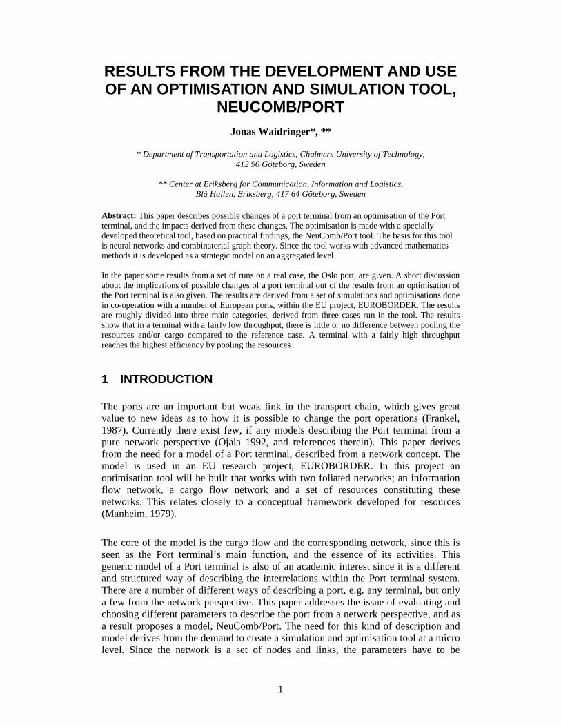
1

RESULTS FROM THE DEVELOPMENT AND USE OF AN OPTIMISATION AND SIMULATION TOOL,

NEUCOMB/PORT

Jonas Waidringer*, **

* Department of Transportation and Logistics, Chalmers University of Technology, 412 96 Göteborg, Sweden

** Center at Eriksberg for Communication, Information and Logistics,

Blå Hallen, Eriksberg, 417 64 Göteborg, Sweden Abstract: This paper describes possible changes of a port terminal from an optimisation of the Port terminal, and the impacts derived from these changes. The optimisation is made with a specially developed theoretical tool, based on practical findings, the NeuComb/Port tool. The basis for this tool is neural networks and combinatorial graph theory. Since the tool works with advanced mathematics methods it is developed as a strategic model on an aggregated level. In the paper some results from a set of runs on a real case, the Oslo port, are given. A short discussion about the implications of possible changes of a port terminal out of the results from an optimisation of the Port terminal is also given. The results are derived from a set of simulations and optimisations done in co-operation with a number of European ports, within the EU project, EUROBORDER. The results are roughly divided into three main categories, derived from three cases run in the tool. The results show that in a terminal with a fairly low throughput, there is little or no difference between pooling the resources and/or cargo compared to the reference case. A terminal with a fairly high throughput reaches the highest efficiency by pooling the resources

1 INTRODUCTION The ports are an important but weak link in the transport chain, which gives great value to new ideas as to how it is possible to change the port operations (Frankel, 1987). Currently there exist few, if any models describing the Port terminal from a pure network perspective (Ojala 1992, and references therein). This paper derives from the need for a model of a Port terminal, described from a network concept. The model is used in an EU research project, EUROBORDER. In this project an optimisation tool will be built that works with two foliated networks; an information flow network, a cargo flow network and a set of resources constituting these networks. This relates closely to a conceptual framework developed for resources (Manheim, 1979).

The core of the model is the cargo flow and the corresponding network, since this is seen as the Port terminal’s main function, and the essence of its activities. This generic model of a Port terminal is also of an academic interest since it is a different and structured way of describing the interrelations within the Port terminal system. There are a number of different ways of describing a port, e.g. any terminal, but only a few from the network perspective. This paper addresses the issue of evaluating and choosing different parameters to describe the port from a network perspective, and as a result proposes a model, NeuComb/Port. The need for this kind of description and model derives from the demand to create a simulation and optimisation tool at a micro level. Since the network is a set of nodes and links, the parameters have to be

2

consistent. The model, which is the result of this paper, is built upon network theory in general and neural3 networks and combinatorial graph theory in particular. Another restriction is that the parameters have to be quantitative, since the network model is based upon mathematical operations. The model as such is a tactical/strategic tool that can be used for long-term reorganisation issues in a Port terminal, since the model is a PC-based optimisation and simulation tool. This means either simulation of physical reconstruction, with corresponding changes in the terminal flow or reorganisation of the work in the Port terminal e.g. changes in the resource distribution. There are two ways of using the tool. The first is to utilise it as an optimisation tool for an already existing Port terminal. The second is to use it as a simulation tool, where it is possible to simulate any given set of parameters in a Port terminal. The simulation is also used as a way of validating the model. The cargo throughput and the resource utilisation are the main issues for optimisation, considering however the constraints implied by information, administration and legal factors. The networks are just a way of explaining abstract interactions and interrelations in the model. The optimisations are done according to the boundary conditions determined by the information, organisation and legal conditions in the Port terminal. The model works with a superposition of three networks, which is though only a way of describing it graphically and in words. In the model/tool, boundary conditions are used to be able to take information, organisation and legal constraints into consideration when optimising, as well as simulating, the Port terminal. The NeuComb/Port tool makes it possible to build a model of any Port terminal with its specific characteristics. The result from the model is either an optimal use of the resources according to a given flow or an optimal flow according to a given set of resources. The utilisation of the resources is also shown. The result is displayed graphically as well as numerically. The tool is made with a generic4 Port terminal model as a demonstration and with default values on all the parameters involved.

3 The part of neural nets that is used in this paper concerns the possibility to store information in both nodes and links 4 Generic is used in the sense of an aggregated, non-specific, model

3

2 FRAME OF REFERENCE - THE PORT First the port environment is described in order to define the port as a part of an overall transport and logistical chain.

Industrial system

Market system

Port system

Transport system

Political system

Supplier system

SupplyDemand

RegulationStimulation

ProductsServices

Services

Demand ProductsServices

RegulationStimulation

RegulationStimulation

Figure 1 The environment of the port (Hulthén and IAHP, 1996) The environmental influence on the port system can be described with activity relations (Figure 1). No detailed description about the port system and how the environment and the port system interact will be done. Instead Figure 1 should be seen as a way of defining the reference system for this paper. Port models used as a base for planning and analysis may be classified in the following way (Ojala, 1992):

• Models with an econometric approach • Models with an analytical approach • Models using simulation technique Econometric models normally deal with the macro-level aspects, and are widely used in research problems related to demand and supply. A system is described as a casual network of relationships between a set of variables. Analytic models are created within the framework of Operations Research (OR). The basic idea is to develop a mathematical function, which can be solved by an algorithm under certain constraints. Simulation models use a numerical technique for specific mathematical models to analyse time-bound flows of events within a system, consisting of a large number of variables and constraints. To provide our model with a background, some examples of how to describe a Port terminal are given, beginning with the terminal as a "black box”, as shown in Figure 2.

4

PORTTERMINAL

CARGOTYPE 1 IN

CARGOTYPE 2 IN

CARGOTYPE 1 OUT

CARGOTYPE 2 OUT

INFORMATIONIN/OUT

RESOURCESIN/OUT

Figure 2 Different flows through the Port terminal The description above is the simplest possible way of describing a Port terminal, in terms of logistical flows. The terminal is seen as a "black box" with cargo, information and resources going in and out of the box. The different flows and their future fate is not taken into account, instead the focus is on the results, i.e. what is actually going in and out of the model. This is in line with the systems approach (Churchman, 1981): “The way to describe an automobile is first by thinking about what it is for, about its function, and not the list of items that make up its structure” Within this frame the Port terminal is described with three main functions, receive/deliver, load/unload and transfer as shown in Figure 3 below.

L o a d /U n lo a d

R e c e iv e /D e liv e r

T ra n s fe r

L a n d s id e P o rt te rm in a l S e a s id e

Figure 3 The Port terminal described by its functions The analytical approach described above is used as a frame of reference for this paper, since the model developed is created as a base and as a tool for simulation and optimisation.

5

3 THE PORT TERMINAL FROM A NETWORK PERSPECTIVE As mentioned before, the model describes the Port terminal as two foliated networks, the information flow network and the cargo flow network, and a set of resources constituting these networks. Figure 4 below shows a few selected nodes and possible links within and between these networks.

INFORMATIONNETWORK

CARGONETWORK

RESOURCES

Resource allocation→

Information exchange→

Link→

Figure 4 The Port terminal’s two foliated networks, and set of resources. The links between the different nodes are not a fixed set of links constantly connecting all the different nodes continuously. Instead the links between two nodes appear when there is a need for a link. In this sense it is possible to talk about links as spontaneous. The links are induced by a need, detected by the information network, which is transferred to the resource network. According to that a resource, i.e. a machine, personnel etc., is assigned to solve that need, creating the desired link. The information, status, from the cargo network is transferred to the information network. It can for example be a need for transportation of the cargo from one node to another. In the information network data is also sent to the next node corresponding to the cargo node receiving the cargo. The resources are limited to use the links available in the cargo network, and when free, placed at a parking area.

Realisable links

Desired links

Realised links

Figure 5 Different sets of links

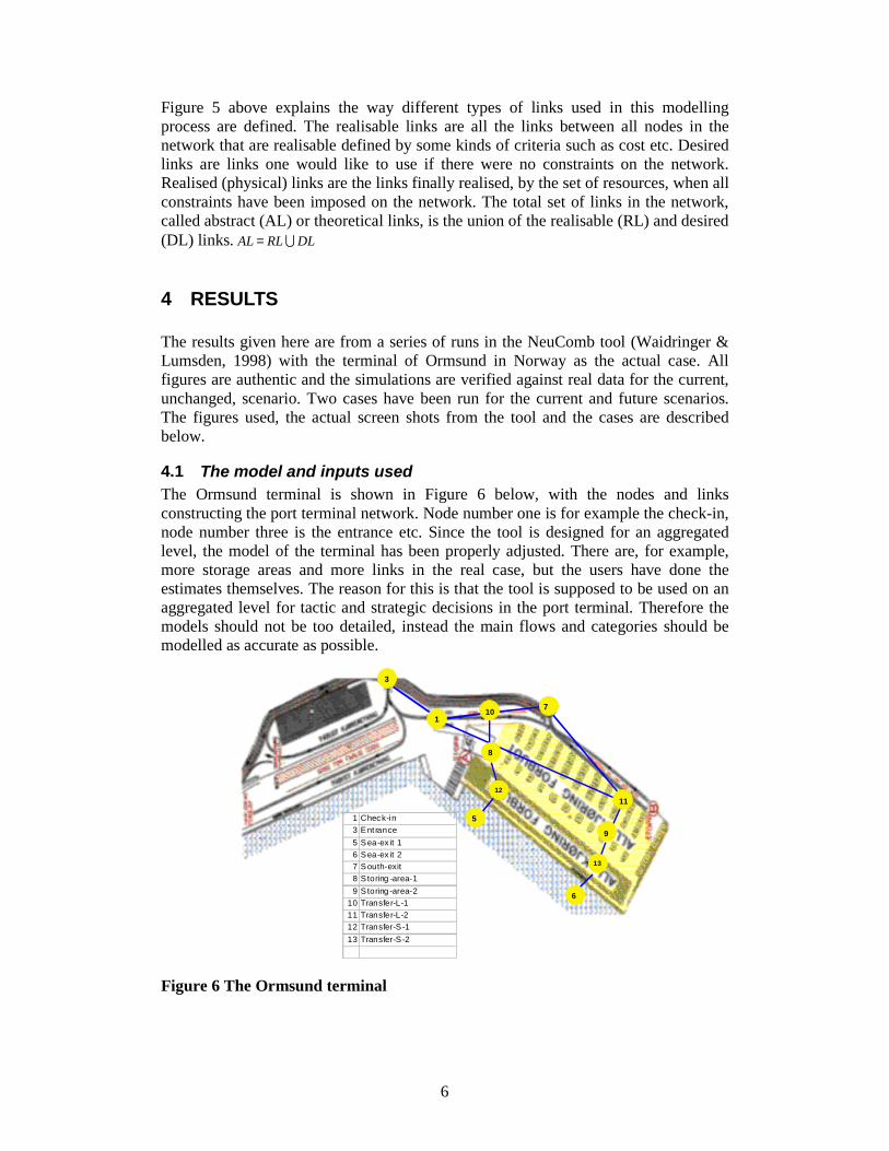
6

Figure 5 above explains the way different types of links used in this modelling process are defined. The realisable links are all the links between all nodes in the network that are realisable defined by some kinds of criteria such as cost etc. Desired links are links one would like to use if there were no constraints on the network. Realised (physical) links are the links finally realised, by the set of resources, when all constraints have been imposed on the network. The total set of links in the network, called abstract (AL) or theoretical links, is the union of the realisable (RL) and desired (DL) links. AL RL DL= �

4 RESULTS The results given here are from a series of runs in the NeuComb tool (Waidringer & Lumsden, 1998) with the terminal of Ormsund in Norway as the actual case. All figures are authentic and the simulations are verified against real data for the current, unchanged, scenario. Two cases have been run for the current and future scenarios. The figures used, the actual screen shots from the tool and the cases are described below.

4.1 The model and inputs used The Ormsund terminal is shown in Figure 6 below, with the nodes and links constructing the port terminal network. Node number one is for example the check-in, node number three is the entrance etc. Since the tool is designed for an aggregated level, the model of the terminal has been properly adjusted. There are, for example, more storage areas and more links in the real case, but the users have done the estimates themselves. The reason for this is that the tool is supposed to be used on an aggregated level for tactic and strategic decisions in the port terminal. Therefore the models should not be too detailed, instead the main flows and categories should be modelled as accurate as possible.

1 Check-in3 Ent rance5 Sea-ex it 16 Sea-ex it 27 South-exit8 S toring -area-19 Storing -area-2

10 Transfer-L-111 Transfer-L-212 Transfer-S -113 Transfer-S -2

3

110 7

11

5

12

9

13

6

8

Figure 6 The Ormsund terminal

7

The basic model, called “current”, is the Ormsund model and the model looks like Figure 7, when it is implemented in the NeuComb tool. The actual tool and its specifications are not described here. (Waidringer & Lumsden, 1998)

Figure 7 The NeuComb tool with the Ormsund terminal lay-out, current situation Figure 7 shows the layout of the terminal, with the check-in at the upper left-hand side corner, corresponding to the layout in Figure 6 above.

To give the reader a possibility to follow the construction of the model and cases, the actual inputs are shown in tables below. It also gives an understanding of the size of the model and cases. The landside distribution for different cargo types in the current and future situations are shown in Table 1 below. Landside distribution means truckloads coming in and out of the terminal over a specified day. Import is going out of the terminal and export is coming in to the terminal from the landside. The tool works with different cargo types, for example imp.-1, imp.-2 etc. to distinguish between cargo destined to different ships, and as a way of determining directions of the flows.

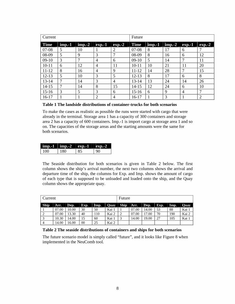
8

Current Future

Time imp.-1 imp.-2 exp.-1 exp.-2 Time imp.-1 imp.-2 exp.-1 exp.-2 07-08 5 10 1 2 07-08 8 17 6 7 08-09 5 9 3 7 08-09 8 16 6 12 09-10 3 7 4 6 09-10 5 14 7 11 10-11 6 12 4 11 10-11 10 21 11 20 11-12 8 16 4 9 11-12 14 28 7 15 12-13 5 10 3 5 12-13 8 17 6 8 13-14 7 14 3 4 13-14 13 24 14 26 14-15 7 14 8 15 14-15 12 24 6 10 15-16 3 5 3 6 15-16 6 9 4 7 16-17 1 1 2 4 16-17 1 3 1 2

Table 1 The landside distributions of container-trucks for both scenarios To make the cases as realistic as possible the runs were started with cargo that were already in the terminal. Storage area 1 has a capacity of 300 containers and storage area 2 has a capacity of 600 containers. Imp.-1 is import cargo at storage area 1 and so on. The capacities of the storage areas and the starting amounts were the same for both scenarios.

imp.-1 imp.-2 exp.-1 exp.-2 100 180 85 90

The Seaside distribution for both scenarios is given in Table 2 below. The first column shows the ship’s arrival number, the next two columns shows the arrival and departure time of the ship, the columns for Exp. and Imp. shows the amount of cargo of each type that is supposed to be unloaded and loaded onto the ship, and the Quay column shows the appropriate quay.

Current Future Ship Arr. Dep. Exp. Imp. Quay Ship Arr. Dep. Exp. Imp. Quay 1 07.00 10.00 30 50 Kai 1 1 07.00 14.00 53 88 Kai 1 2 07.00 13.30 40 110 Kai 2 2 07.00 17.00 70 190 Kai 2 3 10.30 14.00 15 60 Kai 1 3 14.00 19.00 27 105 Kai 1 4 14.00 16.00 00 25 Kai 2

Table 2 The seaside distributions of containers and ships for both scenarios The future scenario model is simply called “future”, and it looks like Figure 8 when implemented in the NeuComb tool.

9

Figure 8 The NeuComb tool with the Ormsund terminal lay-out, future scenario There are two main differences between the current situation and the future scenario. The first is that the amount of cargo of all types is more than double in the future scenario. The second is that there are 4 ships calling at the terminal in the current case and 3 ships in the future scenario. The extra blue lines (links) in figure 3 compared to figure 1 and 2 are links that allow the pooling of resources and cargo.

4.2 The cases run in the model The two models, the current and the future scenario, have been run in the tool with 3 cases in each model: • Case 1, Reference scenario: No changes = two operators and no advanced yard

management system • Case 2: Pooled resources = a single operator • Case 3: Pooled resources and cargo = a single operator and an advanced yard

management

A short clarification The reference scenario is the current situation with no changes to the resources or the cargo. This means that there are external resources (trucks) coming in with the cargo, the cargo is then transferred to internal resources (straddle carriers). Since there are two different companies working in the terminal today the internal resources are divided into two separate areas. The cargo is divided by shipper, Maersk, Greenship etc. Case 2 is a test of the possibility of using a single operator for the internal

10

resources (straddle carrier) in the terminal. The idea is that it should be more efficient and less expensive to pool the resources in the terminal. In practice this means that the internal resources are allowed in the whole terminal. Case 3 is a development of case 2. The idea is that the cargo can be placed anywhere in the terminal. In that way it should be possible to cut down the number of internal resources. To be able to do this an advanced yard management system is required. This kind of system keeps track, in detail, of each container/trailer in the terminal.

The pooling of resources only involves the internal resources (straddle carriers) and not the trucks or cranes. These two cases, number 2 and 3, were seen by the users/operators as the most interesting cases to investigate in more detail. For the Ormsund terminal this is especially true, since they are situated in the middle of Oslo and therefore have a space problem, simply not enough storage capacity in the terminal. They have no opportunities to expand, instead other alternatives have to be considered that enhance the terminals efficiency. The results based on an evaluation of the efficiency figures and queues for the internal resources (straddle carriers) are displayed in a couple of diagrams shown below.

In the EUROBORDER project the resource utilisation was chosen as the main measure, calculated as occupied time/total time, where occupied time means all time the resource (Straddle carrier) is carrying cargo, including the queue time. This measure was agreed on at an early stage of the project and has been kept. The efficiency given in Figure 9 below is a slightly different measure that gives the efficient utilisation of resources at a given throughput and a given set of resources. To be more specific, if we have an identical system regarding throughput volume, available resources and elapsed time, this means that the most efficient solution will carry out the assignments in the shortest time. This gives, bearing in mind the measure above (occupied time/total time), that if the occupied time decreases the utilisation figure as defined above will decline. The most efficient system will therefore have the lowest utilisation figure. This is the basis for the calculations of the efficiency figures given in this document.

To give an example: The resource utilisation figure for case 1 (Unchanged) is 0,25 and the same figure for case 3 (Pooled resources and cargo) is 0,29. This gives a less efficient use of the resource in case 3. As stated above, this discussion is valid for all the figures about efficiency that are given in this paper.

11

Current situation - Efficiency

100 100100,0 100,086,2

96,2

0

20

40

60

80

100

120

Efficiency with queues Efficiency withoutqueues

ReferencePooled resourcesPooled resources & cargo

Figure 9 Efficiency figures for the current scenario The figures are indexed and related to the reference (business as usual) terminal efficiency, which has been given the index of 100.

The reason for this marginal cost reasoning is that if the basic figures for the cases, throughput volume, available resources etc. are the same, the system deviation will be marginal if only the changes are compared. This is a way of compensating for the eventual systematic deviations caused by errors in the figures used for building the models.

Current situation - Queues

0,0 0,0

10,3

0,0

2,0

4,0

6,0

8,0

10,0

12,0

Time in queue

%

ReferencePooled resourcesPooled resources & cargo

Figure 10 Queues for the different cases in the current scenario The percentage in figure 10 shows the percentage of the total time that the resources are standing in queue related to the total occupied time of that resource. As can be seen in the figure, only case 3 causes queues in the system.

12

Some general comments to the current situation: • It is a sparse system with little overall activity, which gives less room for

improvements • Case 2, the pooled resources case and case 1, the reference case give the same

efficiency of resources • Case 3, the pooled resources and cargo case gives less efficient utilisation of

resources and also creates queues • The efficiency figures without queues are almost identical • There are two main bottlenecks in the system, the check-in function and the

container cranes

Future scenario - Efficiency

100 100

118,9

100,0

118,9111,4

0

20

40

60

80

100

120

140

Efficiency with queues Efficiency withoutqueues

Reference

Pooled resources

Pooled resources &cargo

Figure 11 Efficiency figures for the future scenario This figure corresponds to Figure 9 for the current situation, which means that it has the same basis for its construction. The reference case is set to 100 and the other cases are compared to this case. The future scenario’s throughput volume is about double the current situation for all the cargo types.

Future scenario - Queues

10,2

15,9

24,5

0,0

5,0

10,0

15,0

20,0

25,0

30,0

Time in queue

%

ReferencePooled resourcesPooled resources & cargo

Figure 12 Queues for the different cases in the future scenario

13

This figure corresponds to Figure 10 for the current situation, which means that it has the same basis for its construction. Some general comments to the future scenario: • This is a much more dense system with more overall activity, which gives more

room for improvements (and mistakes) • Case 2, the pooled resource case gives better efficiency than unpooled. • Case 3, the pooled resource and cargo case gives the same efficiency as the

reference case, but create more queues than the other two • The efficiency figures without queue show that the two, pooled cases are about

20% more efficient than the reference case for the actual transfers in the system • The two bottlenecks remain, check-in and container cranes and there are overall

more queues in the system • None of the cases can handle all the goods, so the ships can not leave in time. This

is mostly an affect caused by the capacity of the cranes. To conclude, some comments about the results have to be made. In the current situation where the throughput is fairly low, there is almost no difference between the cases except that there are substantially more queues in case 3, the pooled resources and cargo case. This is not intuitively clear. The reason is that when the cargo is pooled the tool will use the basic strategy that is a first come first serve basis. This means that the cargo chose the shortest path and therefor queues will be created. The small difference in efficiency without queues is due to more transhipments of the cargo. For the future scenario, with a much larger throughput, there are queues in all the cases. Here the highest efficiency is reached in the pooled resources case, which is expected since the queues and resource utilisation, is more evenly spread in a basically overloaded system. The pooled resources case gives less efficiency and considerable more queues. The reason is the same that was explained above. The interesting thing is that the efficiency without queues is almost the same. The explanation is that the cargo is more evenly spread in this case, and therefore the internal resources can be utilised better when pooled.

14

5 CONCLUSIONS - FURTHER RESEARCH In this paper the frame of reference, the Port terminal and network theory has been described and finally these two were combined into a network model of a Port terminal. This way of describing a terminal is seen as very useful, and actually any terminal or enterprise functioning in a similar way can be described. It has been presented within the EUROBORDER project, and received positively by users in Port terminals, since they are Port terminal planners and management that work with planning and organisation of ports. By using the network approach, which is a very common metaphor in the society (Casti, 1995), our Port terminal model is easy to understand and useful as basis for discussions. The network approach allows us to break down the model from the aggregated level all the way down to the parameter level. This makes it very transparent and it is easy to choose the level of abstraction or detail needed. The model is flow-oriented which brings it close to reality. Yet, it is very useful from a pure modelling view, as in e.g. programming, where it has been used in the EUROBORDER project.

6 REFERENCES Casti, J. (1995). The Theory of Networks. In: Networks in Action , (Batten D. Casti J. and Thord R. Ed.) Springer-Verlag, Berlin Churchman W.C. (1981). The Systems Approach. Dell Publishing Co. Inc., New York Frankel E.G. (1987). Port Planning and Development. John Wiley & Sons, New York IAHP. (1996). Future Role of Ports in Combined Transport (Hulthén. L. Ed.) IAHP Head Office, Japan. Manheim M.L. (1984). Fundamentals of Transportation Systems Analysis; Volume 1: Basic Concepts, The MIT Press, Cambridge Ojala L. (1992). Modelling approaches in port planning and analysis, Publications of the Turkuu school of economics and business administration, Series A-4:1992, Turkuu Waidringer, J. & Lumsden, K. (1998), Simulation and optimisation of Port terminals, using a network concept, presented, WCTR8, Antwerp

1

A. RESULTS FROM THE RAUMA CASE This appendix is essentially a compilation of an internal report from the EUROBORDER project. It is included as an extension of Paper III giving the results from another of the cases run in the tool, the Rauma port terminal in Finland. Unfortunately no more complete models were possible to test that extensively in the project and the others will therefore be excluded. All figures are authentic and the simulations are verified against real data for the current, unchanged, scenario. Two cases have been run for the current and future scenarios. The figures used, the actual screen shots from the tool and the cases are described below. The results given here are from a series of runs of the tool with the terminal of Rauma as the actual case. Two cases have been run for the current and future scenarios. The figures used, the actual screen shots from the tool and the cases are described and presented below. The Rauma terminal is shown in Figure 1 below, with the nodes and links constructing the port terminal network. The model of the Rauma terminal has been properly adjusted. There are, for example, more storage areas and more links in the real case, but the idea was to have one entire part of terminal for simulation. The reason for this, as already mentioned in the Ormsund case, is that the tool is supposed to be used on an aggregated level for tactic and strategic decisions in the port terminal. Therefore the models should not be too detailed, instead the main flows and categories should be modelled as accurately as possible.

12

354

6 78

910 11

12 13 14

15

1 Entrance2 Check-in3 Land transfer 14 Land transfer 25 Land transfer 36 Storing area 17 Storing area 28 Storing area 39 Sea transfer 110 Sea transfer 211 Sea transfer 312 Sea exit 113 Sea exit 214 Sea exit 315 Land exit

Figure 1 The Rauma terminal

2

The basic model for the current situation in the Rauma case looks like Figure 2 below, when implemented in the NeuComb tool.

Figure 2 The Rauma terminal lay-out, current situation

The figure above shows the lay-out of the terminal, with the entrance at the right-hand side, corresponding to the lay-out in Figure 2 above. The landside distribution for the different cargo types in the current and future situations are the same. Those are shown in table 1 below. The Rauma case is actually the export case of paper rolls transported to the terminal by train (unit is in tons). There are three different cargo types in the terminal. Each of those has their own “line” for the cargo flow. There is also some import cargo, which has not been taken into account in this case, since the amount of import is sufficiently less than the export. The import and export cases also have different processes for handling cargo, because of major differences in cargo type. It is, in other words, a highly imbalanced cargo flow. Table 1 The landside distributions for both scenarios

Current / Future Time Exp_1 Exp_2 07-08 200 200 08-09 200 200 09-10 200 200 10-11 200 200 11-12 200 200 12-13 200 13-14 200

3

Storage area 1 has a capacity of 3500 paper tons and storage area 2 has a capacity of 4500 paper tons for the examined type of cargo. In the future case the capacity is about 25 % of the current capacity, because of the different method for storing. Exp.-1 is export cargo at storage area 1 and so on. The initial cargo amounts in storing areas 1 and 2 are the same for both scenarios.

Exp.-1 Exp.-2 300 610

The seaside distribution for both scenarios is given in table 2 below. The first column shows the ship’s arrival number, the next two columns show the arrival and departure time of the ship, the columns for Exp. and Imp. show the amount of cargo of each type that is supposed to be unloaded and loaded onto the ship, and the Quay column shows the appropriate quay. Table 2 The seaside distributions for both scenarios

Current / Future Ship Arr. Dep. Exp1 Exp2 Imp Quay 1 07.30 10.30 1000 0 0 Exit 1 2 08.00 13.35 0 2010 0 Exit 2

The future pooled scenario model looks like Figure 3 below when implemented in the NeuComb tool.

Figure 3 The Rauma terminal lay-out, future pooled cases

4

A.1 The cases run in the Rauma model The test case in the Port of Rauma focuses on the reorganisation of methods for exporting rolls of paper. Rolls of paper are generally easily damaged in cargo handling. For this reason all unnecessary shifting in the terminal should be minimised. There is one main difference between the current situation and the future scenario. In the future scenario the paper rolls are stored and shipped in cassettes (used for transportation inside the terminal) in order to avoid damage. This causes lack of capacity in warehouses, because the rolls cannot be stored in high stacks. The two models, the current and the future scenario, have been run in the tool with 2 cases in each model:

• Case 1, Reference scenario: No changes = the two cargo streams have their own resources

• Case 2: Pooled resources = all internal resources are used for both cargo streams

The reference scenario is the current situation with no changes to the resources or the cargo. This means that there are external resources (railway cars) coming in with the cargo; then the cargo is transferred to internal resources (cassettes with tug-masters). The internal resources are dedicated to separate streams for each cargo and the cargo is divided by the target country, England, Germany, etc. Case 2 is a test of the possibility of using the internal resources (cassettes with tug-masters) in the terminal, not depending on cargo streams. The intention is to make it more efficient and less expensive to pool the resources in the terminal. The pooling of resources only involves the internal resources (cassettes with tug-masters). The users have regarded the future case as the most interesting case to investigate in more detail. As a result case 2, with pooled internal resources, caused queues in the system and queues occurred in the transfer (land) between train and cassettes. Somehow the resources were not able to serve both streams 1 and 2 impartially. Stream 1 was more efficient (+34 % in loading time) in case 2 than it was in case 1, but stream 2 was not (-44 %). Some general comments on the current situation:

• In Case 2, the pooled resources case and in case 1, the reference case, the efficiency of resources differs quite a lot

• Case 2, the pooled resources case, gives less efficient utilisation of resources and also creates queues.

• There is one main bottleneck in the system, the land transfer, mostly because of different type of transportation (volumes between terminal and rail transportation are different)

• The efficiency without queues is identical between the two cases.

5

Future case - Efficiency

020406080

100120140160

Reference Pooled resources

Figure 4 Efficiency figures for the future scenario

The reference case is set to 100 and the other case is compared to this case. In the future case the efficiency is higher in the pooled case than in the reference case.

Future case - Queues

05

10152025

Reference Pooled resources

Time in queues

%

Figure 5 Queues for the different cases in the future scenario

Some general comments on the future scenario:

• Case 2, the pooled resource case, gives better efficiency than not pooled, but create more queues than the pooled

• The same main bottleneck remains in the system as in the current case, the land transfer, mostly because the different types of transportation (volumes between terminal and rail transportation are different)

In the future scenario the time in queues is a little less than in the current reference case. This is mostly due to the different method of storing. The time for shifting cargo decreases by changing method of storing. Also the differences between pooled and

6

not pooled cases are smaller in the future cases than in the current cases. The reason for this is probably that the terminal processes are not so complicated as in the current situation. In the future cases the cargo can be considered as a special load unit (cassette).