political inequality in affluent democracies · political inequality in affluent democracies: the...
TRANSCRIPT
Political Inequality in Affluent Democracies:
The Social Welfare Deficit
Larry M. Bartels
Department of Political Science
Vanderbilt University
March 2017
DRAFT—Comments welcome
I examine the relationship between public opinion and social spending in thirty
affluent democracies over the past three decades. I find that governments’
responsiveness to citizens’ preferences was highly skewed in favor of affluent
citizens, who were generally less supportive of the welfare state than poor
citizens were. This bias in responsiveness reduced the equilibrium level of social
spending in most countries by 10-15%. Separate analyses of subsets of country-
years differentiated by political culture, democratic consolidation, electoral and
policy-making institutions, national wealth, and economic inequality produced
significant evidence of severe disparities in responsiveness in every case. These
findings suggest that political inequality is rampant in contemporary affluent
democracies.
Presented at a Workshop on Political Inequality and Democratic Innovations
(Democratic Participation—A Broken Promise?), Villa Vigoni, 14-17 March 2017,
and at the 4th Conference in Political Economy & Political Science (Assessing
Democratic Institutions), Toulouse, 23-24 March 2017.
Working Paper 5-2017
Research Concentration: Elections and Electoral Rules

Political Inequality in Affluent Democracies:
The Social Welfare Deficit 1
The preeminent scholar of modern democracy, Robert Dahl (1971, 1), argued that
“a key characteristic of a democracy” is “the continuing responsiveness of the
government to the preferences of its citizens, considered as political equals.” This
understanding has inspired a great deal of empirical research over the past half-
century examining the relationship between citizens’ policy preferences and the policy
choices of elected officials (e.g., Miller and Stokes 1963; Page and Shapiro 1983; Bartels
1991; Stimson, MacKuen, and Erikson 1995; Soroka and Wlezien 2010). According to
one prominent scholar (Shapiro 2011), this research has generated “evidence for strong
effects of public opinion on government policies,” providing “a sanguine picture of
democracy at work.”
Alas, in recent years scholars of American politics (e.g., Gilens 2005; 2012; Bartels
2008; 2016b; Gilens and Page 2014) have produced striking evidence that the apparent
“strong effects” of aggregate public opinion in these studies mask severe inequality in
responsiveness to the preferences of affluent, middle-class, and poor citizens—a
conspicuous violation of Dahl’s stipulation that government should respond to the
preferences of citizens “considered as political equals.” As Martin Gilens (2012, 1) put
it, “The American government does respond to the public’s preferences, but that
responsiveness is strongly tilted toward the most affluent citizens. Indeed, under most
1 Previous versions of the analysis reported here were presented at the University of California-
Berkeley, Nuffield College (Oxford), the University of Wisconsin-Madison, Vanderbilt University,
the 22nd International Conference of Europeanists, Sciences Po, Diego Portales University,
UCLA, Ohio University, Northwestern University, and Rutgers University. I am grateful for
criticism and advice from participants on those occasions and from Christopher Achen, Nate
Breznau, Martin Gilens, Hanspeter Kriesi, David Lewis, Benjamin Page, Efrén Pérez, G. Bingham
Powell, Mitchell Seligson, Stuart Soroka, and Christopher Wlezien.

1
circumstances, the preferences of the vast majority of Americans appear to have
essentially no impact on which policies the government does or doesn’t adopt.”
One possible interpretation of these findings is that the American political system
is anomalous in its apparent disregard for the preferences of middle-class and poor
citizens. In that case, the severe political inequality documented there would
presumably be accounted for by distinctive features of the United States such as its
system of private campaign finance, its weak labor unions, or its individualistic
political culture. On the other hand, it might be the case that severe political inequality
is endemic in affluent democracies, and that detailed studies of other countries would
produce similar results. Unfortunately, research on disparate responsiveness in other
democratic systems is at a very early stage. Thus, the broader relevance of the U.S.
evidence is by no means clear.
My aim here is to test the extent to which policy-makers in a variety of affluent
democracies respond to the preferences of their citizens considered as political equals.
My analysis focuses specifically on the relationship between public opinion and
government spending on social welfare programs, including (for example) old age
pensions, health, education, and unemployment benefits. These programs represent a
major share of government spending in every affluent democracy (Wilensky 2002) and,
arguably, an important source of public well-being (Radcliff 2013). As Gøsta Esping-
Anderson (1990, 106) argued in an influential study of welfare state structures,
“expenditures present a circumspect and possibly misleading picture of welfare-state
differences. If what we care about is the strength of social rights, equality,
universalism, and the institutional division between market and politics, social-
spending levels may camouflage more than they reveal.” Nevertheless, significant
variation across countries and over time in social spending levels is likely to be both
politically salient and economically and socially significant.
2
Another advantage of focusing on social spending is that it figures prominently in
the comparative literature on the political impact of public opinion in affluent
democracies, with major scholarly works suggesting that social spending is
significantly influenced by citizens’ preferences. For example, one prominent account
of Why Welfare States Persist concluded that “mass policy preferences are a powerful
factor behind welfare state output” (Brooks and Manza 2007, 141). Another influential
study of “dynamic representation” concluded that “the people ultimately decide” on
changes in government spending (Soroka and Wlezien 2010, 182), adding that
“representation” is “not the preserve of the attentive few or of a well-heeled elite”
(Soroka and Wlezien 2010, 165). Thus, there is good reason to expect significant
governmental responsiveness to the preferences of citizens in this domain—and even
some reason to expect responsiveness to the preferences of citizens considered as
political equals, notwithstanding the contrary evidence from the United States.
The availability of consistent, concrete data regarding both social spending and
related public opinion provides unusual scope for systematic analysis of policy
responsiveness. My analysis employs data on citizens’ views about social spending and
the welfare state from three major cross-national survey projects—the International
Social Survey Programme (ISSP), the World Values Survey (WVS), and the European
Values Survey (EVS).2 In combination, these three sources provide relevant opinion data
from 160 surveys conducted between 1985 and 2012 in 30 countries, including most
of the established democracies of Western Europe and the English-speaking world, as
well as newer democracies in Eastern Europe, Latin America, and Asia.3
2 Information and data are available from the respective project websites: http://www.issp.org/;
http://www.worldvaluessurvey.org/wvs.jsp; http://www.europeanvaluesstudy.eu/.
3 The complete list of surveys appears in Table A1. The sample is unbalanced, with as many as
eight or nine surveys in some countries (Germany, Great Britain, Spain, Sweden, and the United
States) but only one or two in others (Estonia, Iceland, Israel, and Mexico). Additional country-
3
In Section 1 of this paper I offer theoretical motivation for focusing on the
responsiveness of policy-makers to citizens’ preferences as a test of political equality. I
provide a brief overview of existing research in this area, emphasizing some key
distinctions in the literature—perhaps most importantly, the distinction between
policy responsiveness and policy congruence.
In Section 2 I use survey data from the ISSP Role of Government modules to
document a substantial, persistent unmet demand for social spending among citizens
in affluent democracies. This “social welfare deficit” seems to provide prima facie
evidence that the responsiveness of policy-makers to citizens’ preferences in this
domain is insufficient to produce congruence between preferences and policy—at least
in the estimation of citizens themselves.
In Section 3 I merge survey data on citizens’ views about social spending and the
welfare state with data on governments’ actual social expenditures in an effort to
assess the extent to which policy-makers in affluent democracies respond to public
opinion. My primary measure of policy outcomes in each country-year is total public
social spending per capita (in 2010 U.S. dollars, at purchasing power parity); spending
data are taken from the OECD’s Social Expenditure (SOCX) Database.4
In Section 4 I examine whether policy-makers respond to the preferences of
citizens “considered as political equals.” For each country-year, I tabulate separate
measures of opinion for citizens at the top and bottom of the income distribution and
repeat my analyses of policy responsiveness allowing for the possibility that affluent
and poor citizens have unequal influence.
years are excluded from my analysis because corresponding data on social spending or
economic conditions are unavailable.
4 The average level of social spending in the 141 country-years in my analysis is $6,182 per
capita; the range is from $312 per capita (in South Korea in 1990) to $12,051 per capita (in
Norway in 2007). Descriptions of variables and summary statistics appear in Table A2.
4
In Section 5 I outline a non-linear model of policy-making in which the same
explanatory factors considered in Section 4 are reconfigured to shed light on the
process of dynamic equilibration through which levels of social spending shift in
response to “effective demand” in each country-year reflecting public opinion and
other factors. In addition to illuminating the process of policy responsiveness, this
non-linear model provides a clearer statistical test of the relative political influence of
affluent and poor people in the domain of social spending.
In Section 6 I provide some rudimentary analyses of potential variation in patterns
of policy responsiveness across affluent democracies. I differentiate countries on the
basis of broad political cultures, comparing the “social democracies” of continental
Europe and Scandinavia with the “liberal democracies” of the English-speaking world
and Asia. I also compare countries with different political institutions, allowing for
distinct patterns of policy responsiveness in countries with federal or centralized
systems and proportional or majoritarian electoral systems. Finally, I provide separate
analyses of country-years differentiated on the basis of national wealth and economic
inequality in order to assess whether these economic factors have a discernible impact
on the relative political power of affluent and poor citizens.
My findings suggest two very important caveats to Brooks and Manza’s (2007, 141)
claim that “mass policy preferences are a powerful factor behind welfare state output.”
First, mass policy preferences do not seem to be powerful enough to produce welfare
policies that comport with those preferences. Both direct evidence from citizens’ own
assessments and indirect evidence from observed patterns of policy-making suggest
that affluent democracies spend much less on social programs than they would if
policy-makers were fully responsive to citizens’ preferences in this domain. And
second, the apparent impact of public opinion in this domain seems upon closer
inspection to reflect a highly unequal distribution of political influence, with policy-
makers responding powerfully to the preferences of affluent citizens but not at all (or
5
even negatively) to the preferences of poor citizens. In a domain where affluent and
poor citizens often express very different views, this disparity in apparent influence
has substantial implications for welfare state policies as well as for our understanding
of democratic politics.
1. Policy Responsiveness as a Test of Political Equality
As Sidney Verba and Gary Orren (1985, 15) noted more than thirty years ago,
“Political equality cannot be gauged in the same way as economic equality. There is no
metric such as money, no statistic such as the Gini index, and no body of data
comparing countries.” Thus, until recently, scholarship on political inequality has
generally focused on readily observable differences in citizens’ resources and behavior
as proxies for unobservable differences in political influence. For example, Verba, Kay
Schlozman, and Henry Brady (1995, 14) motivated their monumental study of political
participation, Voice and Equality, by stipulating that “inequalities in activity are likely
to be associated with inequalities in governmental responsiveness” (cf. Schlozman,
Verba, and Brady 2012). Unfortunately, however, social scientists know rather little
about the extent and consistency of the association between political participation and
political influence.5
In the past fifteen years, a variety of scholars employing a variety of data and
research designs have attempted to measure “inequalities in governmental
responsiveness” more directly. Lawrence Jacobs and Benjamin Page (2005) showed that
policy-makers’ views about foreign policy were significantly influenced by business
leaders and experts, but not by the opinions of ordinary citizens. My own analyses of
U.S. senators’ roll call votes found that they were influenced by the preferences of
5 Direct assessments of the impact of participation on political influence have produced mixed
results. For example, U.S. senators seemed to pay more attention to the views of constituents
who contacted them or their staffs, but not to the preferences of those who turned out to vote
(Bartels 2008, 275-280).
6
constituents in the top one-third of the income distribution but not at all by the
preferences of low-income constituents (Bartels 2008, chap. 8; 2016b, chap. 8). Patrick
Flavin (2012, 29) found that “citizens with low incomes receive little or no substantive
political representation (compared with more affluent citizens) in the policy decisions
made by their state governments.” Elizabeth Rigby and Gerald Wright (2013) found
that political parties in the states were generally unresponsive to low-income
preferences. At the national level, Martin Gilens (2005; 2012) used hundreds of specific
policy questions in opinion surveys to show that the likelihood of subsequent policy
shifts was strongly related to the views of affluent citizens, but not to the views of
middle-class or poor citizens when those groups’ policy preferences diverged.
While each of these analyses has significant limitations, the convergence of results
from independent studies employing different data and research designs is impressive;
and the remarkable extent of bias they portray casts considerable doubt on “a
sanguine picture” of American democracy. By comparison, it is hard to point to
credible empirical support for the hypothesis that policy-makers are influenced
equally, or approximately equally, by the preferences of affluent and poor citizens.
Studies purporting to cast doubt on the reality of biased responsiveness have either
been too underpowered to make much of their null results (Bhatti and Erikson 2011) or
motivated by a quite different question—who gets their way rather than whose
preferences matter (Soroka and Wlezien 2008; Enns 2015; but see Gilens 2009; 2015).
Scholars of political representation have long recognized a crucial distinction
between the concepts of proximity—how close or far a representative is from the
preferences of her constituents—and responsiveness—how much their preferences
influence her behavior (Achen 1978). From the standpoint of collective representation,
one might similarly ask how close or far a policy outcome is from the preferences of
citizens or, alternatively, how much citizens’ preferences influence the outcome. The
former is a descriptive feature of the political system; outcomes may reflect citizens’
7
preferences for a variety of reasons having nothing to do with their own political
influence. The latter is a measure of political power in the sense proposed by Achen
(1978, following Nagel 1975). While it is interesting to know who gets their way,
political inequality as I use the term here is a matter of whose preferences matter.
Attempting to infer responsiveness from proximity (or, for that matter, proximity
from responsiveness) is empirically perilous. In the realm of social spending, for
example, policy-makers may respond at the margin to public preferences for spending
increases or decreases, yet continue to spend much less (or much more) than citizens
want. On the other hand, spending may be roughly consistent with citizens’
preferences in an absolute sense (perhaps because policy-makers and citizens
preferences are similarly shaped by economic and social conditions) but unresponsive
to shifts in those preferences if and when they occur. The former situation reflects
responsiveness but not proximity; the latter situation reflects proximity but not
responsiveness.
Critics of the literature on biased responsiveness often conflate this distinction,
assuming that “inequality in representation” requires disparities in proximity across
groups. Since disparities in proximity across groups in turn require differences in the
preferences of those groups, the implication is that “where preferences are identical,
there is no basis for inequality” (Soroka and Wlezien 2008, 319).6 Leaving aside the
empirical question of whether the preferences of relevant groups are (even
approximately) identical (Gilens 2009), this view leaves no meaningful distinction
between Dahl’s notion of “continuing responsiveness of the government to the
preferences of its citizens, considered as political equals” and what Gilens and Page
(2014, 573) referred to as “democracy by coincidence, in which ordinary citizens get
6 If the preferences of different groups are nearly identical, it may be impossible to discern
statistically how much each group’s preferences matter. But that is a practical problem of
inference, not evidence that their preferences matter equally.

8
what they want from government only when they happen to agree with elites or
interest groups that are really calling the shots.”
The theoretical distinction between responsiveness and proximity has important
implications for research design. Perhaps most importantly, it underlines the
importance of assessing the relative influence of different groups’ political preferences
simultaneously within the framework of a reasonably realistic model of the policy-
making process. Soroka and Wlezien’s (2010, 165) claim that “representation” is “not
the preserve of the attentive few or of a well-heeled elite” was based on an analysis
relating policy shifts in the United States and Canada separately to the preferences of
distinct income, education, and partisan groups—assessing, for example, whether
policy “reflects the preferences” of low-income citizens in an analysis where the
preferences of middle- and high-income citizens are ignored, then assessing whether
policy “reflects the preferences” of middle-income citizens in an analysis where the
preferences of low- and high-income citizens are ignored, and so on (Soroka and
Wlezien 2010, 161-167). The results of such analyses obviously cannot tell us which, if
any, of these groups’ preferences actually influenced policy, or to what extent. If
governments only seem to be responsive to the views of ordinary citizens because
those views happen to coincide with the preferences of privileged elites, affluent
citizens, or powerful interest groups, then the appearance of popular political
influence is illusory.
Soroka and Wlezien (2010, 161) noted that more direct attempts to assess the
political influence of specific sub-groups are “complicated by very high
multicolinearity resulting from the substantial parallelism in preferences” across
groups within each country. True enough; but the appropriate response to that
analytical challenge, in my view, is not to sidestep it but to meet it as best we can,
accepting uncertain evidence for what it is worth and hoping that a variety of studies
in different settings employing different research designs will gradually provide a
9
persuasive picture of the contours of political inequality in democratic political
systems.7
Detailed studies of individual countries similar in design to Gilens’ (2012) study of
the United States are currently underway in Germany (by Lea Elsässer and Armin
Schäfer), Sweden (by Mikael Persson and Mikael Gilljam), and Switzerland (Rosset
2016). Studies of this sort will provide considerable insight regarding the ubiquity of
political inequality in affluent democracies. Here, I provide a more superficial but
broader examination of biases in responsiveness in a single policy domain across
dozens of political systems.
Much of the cross-national literature on political representation focuses on
congruence rather than responsiveness, and on broad ideological positions rather than
specific policy issues (e.g., Huber and Powell 1994). Nathalie Giger, Jan Rosset, and
Julian Bernauer (2012, 55) extended this paradigm to consider unequal representation
in 21 democracies in the first decade of the 21st century. They found that “in the
majority of countries, being relatively poor is associated with lower levels of
government congruence.”
Few studies have examined disparities in responsiveness in specific policy areas
cross-nationally. In the work closest in sprit to mine, Yvette Peters and Sander Ensink
(2015) related social expenditures in 25 European democracies to support for
redistribution among high- and low-income citizens (controlling for government
ideology and GDP growth). They interpreted their findings as reflecting “differential
7 Of course, the effect of multicollinearity in this context depends not only upon the correlation
between the preferences of affluent and poor citizens but also upon the total amount of
observed variability in preferences across country-years. The correlations between the
preferences of affluent and poor citizens in my analyses range from R=.83 in the case of social
spending preferences to R=.85 in the case of welfare state values. Nonetheless, as we will see,
the data seem to be quite informative regarding the relative impact of affluent and poor
citizens’ preferences on social spending.
10
responsiveness”; however, their statistical results actually seem to imply that high-
income preferences had no effect on spending (.010 with a standard error of .038),
while low-income preferences had a negative effect (−.088 with a standard error of
.048). These results are puzzling and, taken in isolation, probably not very informative
regarding the extent of political inequality in social spending.
In contrast, my own unpublished analysis of immigration in Europe (Bartels 2016)
produced “some surprising evidence of egalitarian responsiveness” by policy-makers
to the preferences of their citizens. Employing cross-national data on public opinion
and immigration flows in 24 countries from 2002 to 2014, I found that inflows of new
immigrants were strongly responsive to citizens’ support for immigration—and that
the opinions of affluent and poor citizens seemed to be roughly equally consequential.
As far as I know, this is the only study providing positive evidence of egalitarian
responsiveness to the preferences of affluent and poor people (rather than mere
failures to reject the null hypothesis of egalitarian responsiveness due to inadequate
statistical power). Whether the anomalous results reflect the peculiar politics of
immigration in contemporary Europe or flaws in the data or analysis or merely a
statistical fluke remains to be seen.
Finally, an unpublished paper by Michael Donnelly and Zoe Lefkofridi (2014)
provided a broader analysis of the relationship between high- and low-income citizens’
preferences and subsequent policy changes in fifteen distinct policy domains. They,
too, concluded that policy is “tilted toward the preferences of the wealthy.” However,
their analysis pooled fragmentary data from all fifteen policy domains and 36
European countries (ranging from France and Germany to Malta and Albania) in a
single regression analysis with constant coefficients, ignoring the fact that preferences

11
and (especially) policy changes were measured quite differently in each domain.8 Given
the likely heterogeneity of responsiveness to public preferences across these various
domains, settings, and policy outcomes, it seems hard to know how much stock to put
in this highly amalgamated analysis.
2. Evidence of a “Social Welfare Deficit”
Periodically since 1985, the International Social Survey Programme’s (ISSP) Role of
Government modules have included a battery of questions tapping respondents’ views
about spending on a variety of specific government programs. The battery of spending
questions was introduced as follows:
Listed below are various areas of government spending. Please show whether
you would like to see more or less government spending in each area.
Remember that if you say “much more,” it might require a tax increase to pay
for it.
Respondents were asked whether they wanted more or less spending on each of eight
programs: the environment, health, police and law enforcement, education, defense,
old age pensions, unemployment benefits, and culture and the arts. I focus here on the
four programs that cohere most clearly (both theoretically and empirically) in a
common dimension of support for social welfare spending: pensions, health,
education, and unemployment benefits.
By way of illustration, Table 1 shows the distribution of responses to each of these
questions for a single country and year, the United States in 2006. The most striking
pattern here is the strong net public support for increases in social spending. In the
cases of education and health, more than 80% of the survey respondents wanted to
8 Donnelly and Lefkofridi’s measures of policy outcomes ranged from police officers per capita
to “environmental policy intensity and scope” to ratios of tax rates and nuclear energy
production.
12
spend more (or “much more”), while only 4-6% wanted to spend less. In the case of old
age pensions, almost two-thirds of the respondents supported increased spending.
Even in the case of unemployment benefits, which were much less popular than the
bigger-ticket social welfare programs, supporters of increased spending outnumbered
those who wanted to spend less by more than two to one, producing a significant net
public demand for additional spending.
*** Table 1 ***
This substantial public demand for additional social welfare spending is by no
means limited to a single country or a single year. Here, I quantify spending
preferences using a simple scale ranging from zero (for respondents who want to
“spend much less” in a given policy domain) to 100 (for respondents who want to
“spend much more”). A score of 50 represents an equal balance between demands for
spending increases and decreases, while a score in excess of 50 indicates a net demand
for spending increases.9 Averaging the four separate measures of demand for spending
on pensions, health, education, and unemployment benefits provides an overall
measure of social spending preferences.10 Figure 1 summarizes the average net demand
for social welfare spending—demand in excess of the neutral value of 50 on the 0-to-
100 scale—in each of the 25 countries included in my analysis of the ISSP data.11 In
9 The length of the scale is, of course, arbitrary. However, the midpoint on the scale (for
respondents who want to “spend the same as now”) is meaningful, corresponding to
satisfaction with the perceived status quo spending level.
10 Specific measures of demand for spending on pensions, health, and unemployment benefits
can be related to subsequent spending shifts in those specific domains; however, analyses
along those lines (not reported here) generally support Brooks and Manza’s (2007, 143) claim
that “Politicians tend to incorporate mass opinion into social policymaking in a global fashion,
rather than adjusting each specific domain to match precisely citizen preferences.”
11 In countries with multiple ISSP surveys, Figure 1 reports the average net demand across
waves, with fixed effects for the first three waves to capture general shifts in spending
preferences over time in the OECD as a whole.

13
every country, the figure indicates significant demand for increased social spending.
The average values range from 10 or more in the “best” cases (France, the Netherlands,
and Switzerland) to more than 25—the equivalent of a unanimous public desire to
“spend more” in all four social policy domains—in the “worst” cases (Chile, Ireland,
Israel, Portugal, and Poland).
*** Figure 1 ***
In four countries—Australia, Germany, Great Britain, and the United States—the
ISSP spending questions have been asked four times over a period of two decades or
more. Repeated measurement of spending preferences using similar study designs and
identical questions makes it possible to track the magnitude of the social welfare
deficit over time in these four countries. The results are presented in Figure 2. In three
of the four countries, net unmet demand for social welfare spending increased
substantially over time. Only Great Britain saw a significant decline, from very high
levels under Conservative prime ministers Margaret Thatcher and John Major to a
much lower level after nine years of Tony Blair’s Labour government.
*** Figure 2 ***
Lest these four countries be considered anomalous, it is also possible to track
unmet demand for social welfare spending in a broader set of fifteen countries over
the decade between the mid-1990s and the mid-2000s.12 Again, the results produce no
evidence of convergence between spending preferences and policies. Indeed, the
average net demand for social spending in these countries increased by about 10%
between the mid-1990s and the mid-2000s; increases outnumbered decreases by nine
to six.
12 Australia, Canada, the Czech Republic, France, Germany, Great Britain, Ireland, Japan, New
Zealand, Norway, Poland, Spain, Sweden, Switzerland, and the United States.

14
According to Soroka and Wlezien (2010, 173), it is “not surprising” to observe
discrepancies between citizens’ preferences and policies at any given time due to
fluctuations in partisan control of government and other factors: “substantial
disjunctures with public preferences in the short term can exist even as policy reflects
those preferences over the long term.” However, persistent mismatches between
preferences and policies over periods of ten or twenty years seem much harder to
account for within the framework of dynamic representation, which implies that
responsiveness by public officials to citizens’ demands—and recognition of that
responsiveness by citizens—should erode “substantial disjunctures … over the long
term.” The large, persistent social welfare deficits evident in the ISSP data suggest that
one or both of these reciprocal connections must often fail in practice.
3. Policy Responsiveness
The ISSP survey data demonstrate that most citizens in affluent democracies over
the past thirty years have wanted their governments to spend more—often much
more—on a variety of major social programs. Moreover, these preferences for
additional spending have generally persisted over long periods of time. How does that
fact square with Soroka and Wlezien (2010, 128) claim that “When the public wants
more social spending policymakers usually provide it”?
The key to resolving this apparent paradox is to bear in mind that responsiveness
is a matter of degree. Even a “responsive” policy-making process may fail to reflect
public preferences, even over long periods of time, if the extent of responsive is
inadequate. Indeed, this sort of persistent incongruence between public preferences
and policy is evident in Soroka and Wlezien’s own data. At one point, they presented a
graph relating annual changes in social spending in the U.S. to public spending
preferences (based on responses to questions similar in form to those employed here)
in the preceding year (Soroka and Wlezien 2010, 128). The correlation between the two
15
series over the 33 years covered by their analysis is R=.61, suggesting a consistent
pattern of responsiveness. However, the two series are substantially offset in the graph
in order to make them overlap, with a net spending preference of zero implying an
annual decline in social spending of about $35 billion (2000 dollars) and a net
spending preference of more than 20 (corresponding to a net demand of more than 10
in my Figure 1) required to maintain social spending at its current level (adjusted for
inflation, but with no allowance for population growth or growth in per capita income).
The relationship is one of fairly consistent marginal responsiveness, but persistent
incongruence between preferences and policy.13
In this section, I attempt to shed light on the extent of policy responsiveness to
public opinion in the realm of social spending. I begin, in the spirit of the literature on
dynamic representation, with a simple description of the relationship between public
support for social spending in each country-year and subsequent changes in actual
spending levels. Are policy changes correlated with citizens’ spending preferences? In
order to allow time for policy changes to be implemented, I consider changes in
spending over the two years following each ISSP survey.14
The statistical results presented in the first column of Table 2 summarize the
simple bivariate relationship between public support for social spending and
subsequent changes in spending (Model 1). The parameter estimate of .349 implies
13 Most studies of dynamic representation measure public preferences and policies on
incommensurate scales, providing no clear way to assess the degree of congruence between
what citizens want and what they get. The specific survey questions employed by Soroka and
Wlezien (2010)—in which preferences for “more” or “less” government spending in a given
domain are implicitly calibrated to current spending levels—do provide indirect evidence
regarding (in)congruence, but their analyses did not exploit that fact.
14 Since some surveys were conducted toward the end of the indicated calendar year, and since
national policy-making processes vary considerably in their timing, it seems unrealistic to
require that public demand for social spending in year t be translated into additional spending
in year t+1. Thus, I allow policy-makers in year t+1 to respond to demand in year t, producing
changes in spending in year t+2 relative to those in year t.
16
that a difference of 6 points (one standard deviation) in aggregate public support for
social spending was associated with an expected difference of about two percentage
points in incremental spending over the next two years. On its face, this association
seems to provide solid evidence that “budgetary policy responds to public
preferences” (Soroka and Wlezien 2010, 142).
*** Table 2 ***
Figure 3 provides a graphical representation of this relationship between spending
preferences in each country-year and subsequent shifts in spending. One normatively
attractive feature of the relationship is that the regression line seems to imply that a
net public demand of 0—a balance between public preferences to increase social
spending and to decrease social spending—would produce a stable level of spending,
in contrast with the eroding level of spending implied by Soroka and Wlezien’s (2010,
128) analysis. On the other hand, it is clear from the scatterplot that the positive
relationship between spending preferences and subsequent increases in spending is
attributable in large part to just two country-years, Chile and Ireland in 2006.
Excluding these two country-years from the analysis reduces the slope of the
regression line by more than half (as reflected by the dashed line in Figure 3); the
adjusted R2 statistic falls from .14 to .01.15 Thus, the solid evidence of responsiveness
presented in the first column of Table 2 turns out to be rather less solid than it seems.
*** Figure 3 ***
The more elaborate statistical analysis reported in the second column of Table 2
(Model 2) sheds some additional light on the bivariate relationship between public
preferences and budgetary policy. Model 2 includes a variety of factors that might be
15 The regression parameter estimate with these two observations excluded is .143 (with a
standard error of .114).
17
expected to affect social spending regardless of public opinion, including the
dependency ratio (the population of retirement age relative to the population of
working age), national wealth (as measured by the natural log of GDP per capita), and
short-term changes in GDP and unemployment (Wilensky 2002). Once these factors are
taken into account, the apparent effect of public demand on spending two years later
is reduced by about 40%.16 That fact suggests that the bivariate relationship between
public preferences and policy—such as it is—is in large part spurious, with shifts in
spending driven by considerations that shape the preferences of both citizens and
policy-makers.
One possible reason for policy-makers to resist public demands for increased
social spending is that the public support for spending increases apparent in Table 1
(and more broadly in Figure 1) may be offset by concerns about the fiscal cost of an
expansive welfare state. Indeed, evidence from the ISSP Role of Government surveys
themselves suggests that public enthusiasm for social welfare spending coexists with a
strong contrary impulse to curb government spending. In the context of a battery of
questions focusing on “some things the government might do for the economy,”
respondents were asked whether they favored or opposed “cuts in government
spending.”17 In response to this question, the same respondents who expressed
substantial support for additional spending on the social programs that make up the
lion’s share of their governments’ budgets also expressed substantial enthusiasm for
cuts in government spending.18 Indeed, the distribution of responses to the budget-
16 In this specification, excluding Chile and Ireland in 2006 leaves no evidence at all of
responsiveness to public opinion; the regression parameter estimate for social spending
preferences with these two observations excluded is −.025 (with a standard error of .078).
17 The other items in the battery asked about controlling wages and prices, financing projects to
create new jobs, reducing regulation of businesses, supporting industrial research and
development, supporting declining industries to protect jobs, and reducing the work week.
18 The apparent contradiction between public enthusiasm for cuts in government spending and
strong support for increases in spending on specific social programs is heightened by the

18
cutting question is, if anything, even more skewed than for the questions on spending
for specific government programs. Averaging across countries and years, about two-
thirds of the respondents said they favored cuts in government spending, many
“strongly”; only 10% were opposed.
It is worth noting that budget-cutting preferences were only weakly related to
social spending preferences at the aggregate (country-year) level (R=−.25). The
countries with the greatest enthusiasm for budget-cutting include some, like France
and Japan, with relatively low levels of net demand for social spending but also some,
like Hungary and Portugal, with high levels of unmet demand for spending. The
countries with the lowest average levels of support for budget-cutting—Finland,
Denmark, and Britain—had moderate levels of unmet demand for social spending.
Is there any evidence that policy-makers were responsive to their citizens’ budget-
cutting preferences? Models 3 and 4 in Table 2 parallel Models 1 and 2, but with
budget-cutting preferences included along with spending preferences as potential
influences on social spending. Both analyses provide some evidence of responsiveness
to budget-cutting preferences, though the estimated effects are rather imprecise and
smaller in magnitude than those for spending preferences.19 Meanwhile, the apparent
impact of spending preferences on actual spending is not much affected by including
budget-cutting preferences in the analysis.
Table 3 presents additional statistical analyses paralleling those in Table 2, but
with a broader measure of public support for the welfare state. In their influential
proximity of these questions in the ISSP surveys: the spending battery consistently appeared
just six questions after the item about cutting government spending. Thus, within a matter of
two or three minutes the same survey respondents who were fervent budget hawks became
strong supporters of increased spending on a variety of major social programs.
19 Model 4 suggests that an increase of 6 points (one standard deviation) in spending
preferences would increase social spending two years later by about 1.1%, while an increase of
10 points (one standard deviation) in budget-cutting preferences would decrease social
spending two years later by about 0.5%.

19
analysis of Why Welfare States Persist, Brooks and Manza (2007, 39-41) measured
“mass policy preferences” using two more questions included in the ISSP Role of
Government surveys. One of these questions asked, “On the whole, do you think it
should or should not be the government’s responsibility to provide a job for everyone
who wants one?” The other asked, “On the whole, do you think it should or should not
be the government’s responsibility to reduce income differences between the rich and
the poor?” In order to distinguish the more general attitudes toward the welfare state
tapped by these questions from the specific, concrete policy preferences tapped by the
domain-specific spending questions, I shall refer to Brooks and Manza’s “mass policy
preferences” as a measure of support for the welfare state.20
*** Table 3 ***
Brooks and Manza (2007, 36) showed that these attitudes toward the welfare state
were strongly correlated with countries’ welfare state spending (measured as a
percentage of GDP). As Lane Kenworthy (2009) and Nate Breznau (2014) have pointed
out, it is hard to know what to make of this correlation. Cross-national differences in
welfare state effort tend to be rather stable over long periods of time, making it very
difficult to discern whether supportive public attitudes are a cause or an effect of
government policy. I shall attempt to shed some light on that causal ambiguity. In the
meantime, however, it seems plausible to suppose that broad welfare state values may
be more relevant than specific policy preferences in shaping social spending.
The statistical analyses presented in Table 3 allow for the possibility that policy-
makers responded to these broad “embedded preferences … grounded in a country’s
social structure, major institutions, and the collective memory of citizens” (Brooks and
20 My index of welfare state support is a simple average of responses to the two items, rescaled
to range from zero (for respondents who “disagree strongly” with both items) to 100 (for
respondents who “agree strongly” with both items).
20
Manza 2007, 7) rather than to specific, concrete preferences for more or less spending
in any given domain at any given time. More prosaically, they also allow for the
possibility that the measure of spending preferences derived from the ISSP survey data
fails, for one reason or another, to reflect politically relevant aspects of public opinion
regarding social spending.
Model 5 presents the simple bivariate relationship between public support for the
welfare state and subsequent changes in social spending. In contrast to the parallel
relationship for social spending preferences in Model 1, there is virtually no
correlation between public support for the welfare state and subsequent shifts in
policy. However, allowing for the same set of additional influences on social spending
as in Model 2 actually bolsters the apparent impact of public opinion on policy (Model
6). This analysis implies that a difference of 12 points (one standard deviation) in
aggregate public support for the welfare state was associated with an expected
difference of 1.2 percentage points in incremental spending over the next two years.
Finally, Models 7 and 8 examine the combined effects of public support for the
welfare state and for government budget-cutting on subsequent shifts in social
spending. As with Models 5 and 6, adding demographic and economic factors to the
analysis (in Model 8) produces much clearer evidence of a relationship between public
support for the welfare state and actual social spending than in the simpler analysis
focusing solely on public opinion (Model 7). Indeed, this version of the analysis
accounts for shifts in social spending slightly better than the parallel analysis (Model
4) employing concrete social spending preferences. Moreover, allowing for the greater
variability across country-years in public support for the welfare state, the implied
effect of public opinion on policy is slightly larger in magnitude. These results suggest
that welfare state support is a reasonably good proxy for social spending preferences
in accounting for policy changes.
21
Substituting welfare state support for spending preferences as a measure of public
opinion has the practical advantage of expanding considerably the range of cases
available for analysis. While the ISSP data on spending preferences cover 51 country-
years, cross-national data on public attitudes toward the welfare state are rather more
plentiful. Here, I employ data from the World Values Survey (WVS) and European
Values Survey (EVS) to further explore the relationship between public opinion and
social spending in affluent democracies. These surveys include an item roughly
comparable to the ISSP items on the government’s responsibility to provide jobs and
reduce income differences. WVS/EVS survey respondents were invited to place
themselves on a 1-to-10 scale with one endpoint labeled “Government should take
more responsibility to ensure that everyone is provided for” and the other endpoint
labeled “People should take more responsibility to provide for themselves.” Responses
to this item provide a measure of welfare state support for 106 country-years,
including 89 for which ISSP data are unavailable.21
The analyses presented in Table 4 use the WVS/EVS opinion data to explore the
robustness of the relationship between public opinion and social spending in affluent
democracies. On the whole, these analyses cast additional doubt on the notion that
“mass policy preferences are a powerful factor behind welfare state output” (Brooks
and Manza 2007, 141). The bivariate relationship (Model 9, in the first column of Table
4) is positive but statistically unreliable; welfare state support alone does almost
nothing to account for shifts in social spending. Adding the same demographic and
economic factors as in Tables 2 and 3 (Model 10) reduces the standard error of the
analysis substantially (producing an adjusted R2 statistic of .50), but the estimated
effect of public support for the welfare state is perversely negative.
21 The World Values Survey includes data from many other countries, but my analysis is limited
to the affluent democracies for which spending and other data are available from OECD.
22
*** Table 4 ***
Model 11 introduces a different sort of statistical control, with fixed effects for
each of the 30 affluent democracies for which I have data. This (admittedly blunt)
allowance for stable national differences in political culture, governmental capacity,
and economic and social conditions again produces a perversely negative (and
statistically unreliable) estimate of the effect of public support for the welfare state.
Finally, Model 12 includes both demographic and economic variables and country fixed
effects; here, the estimated effect of public support for the welfare state is once again
positive, but once again modest in magnitude and statistically unreliable.
Taken together, the various statistical analyses presented in Tables 2, 3, and 4
provide strong evidence of regularities in social policy-making. Higher levels of
national wealth (as measured by GDP per capita) are consistently associated with
substantial increases in social spending, while higher levels of social spending
significantly dampen the enthusiasm of policy-makers for further increases. (That
equilibrating tendency plays a key role in the dynamic model of policy-making outlined
in Section 5.) Short-term changes in unemployment rates are consistently associated
with changes in spending (with a 1% increase in unemployment producing an increase
of about 1% in social spending). Somewhat less consistently, higher levels of
demographic dependency (as measured by the ratio of retirement-age to working-age
people) seem to be associated with higher levels of social spending.
What these analyses do not provide is much clear statistical evidence of policy
responsiveness to the preferences of citizens. The strongest-looking evidence of
responsiveness (in Table 2) turns out to hinge crucially on just two unusual country-
years, and erodes further when demographic and economic factors are included in the
analyses. Parallel analyses focusing on public support for the welfare state rather than
specific spending preferences (in Table 3) are likewise sensitive to the inclusion of
23
control variables, and the apparent effects of public opinion are even more variable
(and statistically imprecise) when the analyses are replicated in a broader set of
country-years (Table 4). If “mass policy preferences are a powerful factor behind
welfare state output” (Brooks and Manza 2007, 141), they must matter in ways that are
not well captured in these analyses.
4. Disparities in Responsiveness
So far, I have treated public preferences in each country-year as an
undifferentiated force influencing (or failing to influence) subsequent shifts in social
spending. However, the U.S. evidence of disparities in responsiveness to the
preferences of affluent, middle-class, and poor people suggests that the implicit
assumption in analyses of this sort—that all citizens’ views are equally consequential
in the policy-making process—may be quite unrealistic. In this section I provide a more
flexible analysis of responsiveness allowing for the possibility that the political
influence of citizens is correlated with their economic circumstances.
Of course, the substantive implications of disparities in responsiveness will
depend in significant part on the extent to which the preferences of affluent and poor
citizens diverge. If poor citizens have the same preferences as affluent citizens do,
even a very class-biased policy-making process might turn out to give them what they
want, albeit by coincidence. One might—and I would—attach considerable theoretical
and moral significance to the class bias, nonetheless. But from a practical standpoint,
it would have little impact on policy outcomes. On the other hand, if affluent and poor
citizens have very different preferences, a political system skewed in favor of the
affluent will tend to produce policies that fail to reflect the preferences of the poor,
compounding procedural inequality with substantive biases in policy outcomes.
Here, I measure high-income preferences and low-income preferences in each
country-year by regressing survey respondents’ social welfare preferences on their
24
positions in the national income distribution.22 Figure 4 shows the average level of
support for social spending among high-income and low-income respondents in each
country-year covered by the ISSP surveys. In every case, majorities of both affluent and
poor citizens favored increased spending on major social programs, with average
support ranging from 52.7 to 87.5 on the 0-to-100 scale. However, it is clear from the
scatterplot that, in most cases, affluent people were distinctly less enthusiastic about
spending increases than poor people were. On average, this gap in preferences
amounted to 7.3 points—a bit more than one standard deviation in the cross-country
distribution of preferences. In the most extreme case (the United States in 1985),
affluent people were almost 15 points less supportive of social spending than poor
people were. On the other hand, in just two cases (Hungary in 1990 and Korea in 2006)
affluent people were slightly more supportive of social spending than poor people
were.
*** Figure 4 ***
Figure 5 shows the average levels of support for the welfare state among high- and
low-income respondents in each ISSP survey. The cross-national variation in opinion is
considerably greater for welfare state values than for social spending preferences,
especially among affluent citizens. The disparities in preferences between affluent and
poor citizens are also much greater, ranging from 5.6 points (in Chile in 2006) to
almost 40 points (in New Zealand in 1997). In most cases, the disparities in preferences
between affluent and poor citizens were largest in the countries where the overall level
22 In each country-year, I used the most detailed available measure of respondents’ family
incomes (or, if necessary, the respondents’ own incomes) to estimate their place in the income
national distribution. I then regressed each measure of social welfare preferences on income
percentiles separately in each country-year. The predicted preferences at the 1st and 100th
income percentiles are my measures of low- and high-income preferences, respectively, for each
country-year. (I also examined quadratic relationships between preferences and income, but
they generally did little to improve upon the simple linear regressions.)
25
of public support for the welfare state was lowest, including the U.S., New Zealand, and
Canada. However, large disparities in preferences also appeared in some countries with
high levels of overall support, including the Netherlands, Sweden, and France.
*** Figure 5 ***
Figure 6 shows the distribution of welfare state preferences among affluent and
poor citizens in the WVS/EVS surveys. Here, the disparities in preferences between
those at the top and those at the bottom of the income distribution are generally
smaller than in the ISSP surveys—perhaps because the WVS/EVS question about the
government’s responsibility “to ensure that everyone is provided for” does not refer
explicitly to reducing income differences between the rich and the poor in the process.
Nonetheless, there are only a handful of country-years (one in Sweden, two in Spain,
and two in South Korea) in which affluent citizens expressed as much or more support
for the welfare state as poor citizens did. In the remaining 95% of the cases, affluent
people were less supportive of the welfare state than poor people were. The average
difference in support between those at the top of the income distribution and those at
the bottom was 12 points, and in ten cases the difference was more than 20 points.23
Moreover, the average magnitude of the disparity in preferences between affluent and
poor people increased substantially over time, from about 9 points in 1990 to 15
points in 2012.24
*** Figure 6 ***
23 It is interesting to note that the ten largest disparities between the opinions of affluent and
poor people come from ten different countries—Chile, the U.S., Australia, Hungary, Germany,
Slovenia, Poland, Estonia, the Czech Republic, and Sweden.
24 This estimate of change over time is derived from a linear regression analysis of the
difference in preferences between high-income and low-income people in each country-year on
the date of the survey with fixed effects for countries; thus, it is not a reflection of changes in
the set of countries included in the WVS/EVS or of specific political or economic conditions in
1990 or 2012.
26
With differences in opinion of this magnitude, significant disparities in the
political influence of affluent and poor citizens are likely to translate into significant
differences in policy outcomes. But are policy-makers more responsive to the
preferences of affluent citizens than to the preferences of the poor?
Table 5 presents the results of analyses paralleling those in Table 2, but with
separate estimates of policy responsiveness to the spending preferences of affluent
and poor citizens. In the simplest version of the analysis, Model 13, the sum of the
separate coefficients for high-income spending preferences and low-income spending
preferences is similar in magnitude to the single coefficient for spending preferences
in Model 1 in Table 2; but the coefficient for high-income preferences is 6.5 times as
large as the coefficient for low-income preferences.25 With demographic and economic
factors included in the analysis, in Model 14, the sum of coefficients is again similar in
magnitude to the single coefficient in Model 2 in Table 2; but the coefficient for high-
income preferences is 3.2 times as large as the coefficient for low-income preferences.
While these separate parameter estimates for high- and low-income preferences are
quite imprecise, they suggest that policy-makers probably responded much more
strongly to the preferences of affluent citizens than to the preferences of poor
citizens.
*** Table 5 ***
Models 15 and 16 include separate measures of budget-cutting preferences among
affluent and poor citizens in addition to the separate measures of social spending
25 Since “high-income” and “low-income” spending preferences in each country-year are the
endpoints of a linear relationship, we can think of each citizen’s influence on policy as being
proportional to a weighted average of these two endpoints. So the parameter estimates of .286
and .044 in Model 13 imply that a citizen at the 75th percentile of the income distribution had
almost four-fifths as much influence as someone at the top of the income distribution
(.286×.75+.044×.25=.226), while someone at the 25th percentile had a little more than one-third
as much influence as someone at the top of the distribution (.286×.25+.044×.75=.104).
27
preferences. The resulting estimates of the impact of high-income spending
preferences are slightly larger than in the first two columns, while the estimates of the
impact of low-income spending preferences are slightly smaller (indeed, in the third
column, negative). Meanwhile, budget-cutting preferences seem to have their own
independent effect on policy, with again some (albeit less) apparent bias in
responsiveness toward the preferences of high-income people.
The analyses reported in Table 6 parallel those in Table 3, except that the variables
measuring overall welfare state values and budget-cutting preferences are replaced by
separate variables measuring affluent and poor citizens’ welfare state values and
budget-cutting preferences. Again, the parameter estimates reflecting responsiveness
to affluent citizens’ views have the expected signs (positive for welfare state values,
negative for budget-cutting preferences), plausible magnitudes, and fair precision (with
t-statistics ranging in magnitude from 1.4 to 1.9). However, the parameter estimates
reflecting responsiveness to poor citizens’ views are all perversely signed (negative for
welfare state values, positive for budget-cutting preferences), and statistically
“insignificant.” Here, too, the results suggest that poor citizens had essentially no
influence on social spending in affluent democracies.
*** Table 6 ***
Table 7 reports the results of analyses paralleling those in Table 4, but with
separate measures of support for the welfare state among high- and low-income
people in each country-year covered by the WVS/EVS data. In every case, the apparent
effect of affluent people’s views on subsequent shifts in social spending is substantial
(though not always sufficiently precisely estimated to be “statistically significant”),
while the apparent effect of poor people’s views is negative. The persistence of this
pattern across the four distinct analyses, regardless of the presence or absence of
demographic and economic control variables or fixed effects for countries, is
28
noteworthy. These results echo those presented in Tables 5 and 6 in suggesting that
the dramatic inequalities in responsiveness documented by Gilens (2012) and others in
the U.S. are endemic in affluent democracies, posing a major challenge to the ideal of
political equality.
*** Table 7 ***
5. The Policy-Making Process: Dynamic Equilibration
The statistical evidence reported in Tables 5, 6, and 7 implies that social spending
in contemporary affluent democracies responds to the preferences of their most
affluent citizens, but that the preferences of less affluent citizens have little, if any,
impact on policy outcomes. In this section I attempt to shed clearer light on the nature
of that disparate responsiveness by embedding the statistical evidence in a more
explicit dynamic model of the policy-making process. The model represents changes in
social spending in any given country over any given two-year period as the results of a
process of dynamic equilibration between the “effective demand” for spending and the
prevailing spending level:
(1) (ΔSpending i,t+2) = λ[(Effective demandit) – (Spendingit)] + δi,t+2
“Effective demand” represents an equilibrium rate of social spending in country i
in year t based on a variety of political, economic, and other factors. Policy-makers may
act (or not) to reduce the gap between the effective demand for spending and the
actual spending level at any given time. The parameter λ in Equation 1 reflects the
extent to which any gap between effective demand and the current level of spending is,
in fact, reduced over the subsequent two years. Positive values of λ imply that social
spending is likely to increase when the effective demand exceeds the prevailing

29
spending rate and to decrease when the prevailing spending rate exceeds the effective
demand.26
Equation 2 relates the “effective demand” for social spending in each country-year
to prevailing national conditions. The equilibrium rate of spending is assumed to
reflect, in part, the public attitudes toward the welfare state captured in the ISSP and
WVS/EVS survey data. It may also be affected by demographics (measured here by the
dependency ratio of retirement-age people to working-age people), national wealth
(measured by the natural logarithm of GDP per capita), and durable features of each
country’s history, culture, geography, and political structure (captured by fixed effects
for countries):
(2) (Effective demandit) = β1(Public opinionit) + β2(Dependency ratioit) + β3(GDP/capitait) +
α(Countryi)
In order to allow for possible disparities in responsiveness to the views of affluent
and poor people, Equation 3 further specifies the relevant public opinion in each
country-year as a weighted combination of the views of high-income and low-income
citizens:
(3) (Public opinionit) = (High-income opinionit) + ω(Low-income opinionit)
The parameter ω in Equation 3 represents the relative weight attached to the views of
low-income citizens. If ω =1, the opinions of affluent and poor people (and, by
assumption, those in between) are equally important in determining the effective
demand for social spending in any given country-year; if ω=0, the poorest people have
26 This framework is essentially an error correction model (Engle and Granger 1987), with
“equilibration rates” corresponding to the error correction rate and the terms in square
brackets representing the equilibrium relationship between social spending levels and public
preferences and other political and economic factors.
30
no influence at all (and, by assumption, those in between have correspondingly less
influence than those at the top of the income distribution).27
Finally, short-term changes in economic conditions (GDP and unemployment) may
produce changes in social spending independent of the equilibrium relationship
between “effective demand” and actual spending at any given time:
(4) δi,t+2 = γ1(ΔGDP/capitai,t+2) + γ2(ΔUnemploymenti,t+2) + εi,t+2 .
These additions to the model are intended to capture the impact of “automatic
stabilizers” in contemporary welfare states that may produce changes in spending in
direct response to changing economic conditions, with no explicit decisions by policy-
makers. For example, if workers who lose their jobs are automatically eligible for
unemployment benefits, changes in unemployment rates will produce more or less
immediate changes in social spending independent of any effort by policy-makers to
respond to public opinion as it existed before the change.
Substituting Equation 3 into Equation 2 and Equations 2 and 4 into Equation 1
produces a non-linear relationship between year-to-year changes in social spending
and the same explanatory variables included in the analyses reported in Tables 6 and
7. That non-linear relationship forms the basis for the analyses presented in Table 8.
Indeed, the non-linear regression parameter estimates in Model 25 are simply an
algebraic rearrangement of the linear regression parameter estimates in Model 24 in
Table 7. All of the explanatory variables are the same, and in sum they account for
27 Given this parameterization, and the fact that high- and low-income preferences are defined
by a linear regression of policy preferences on relative income levels, the implied
responsiveness of policy-makers to the preferences of middle-income citizens is β1(1+ω)/2. The
implied average level of responsiveness to the preferences of citizens in the top half of the
income distribution is β1(3+ω)/4, while the implied average level of responsiveness to the
preferences of citizens in the bottom half of the income distribution is β1(1+3ω)/4.
31
changes in social spending exactly as well (with a standard error of 4.61) with the same
number of free parameters.
*** Table 8 ***
The reconfiguration of variables and parameters in Model 25 sheds clearer light on
the process of dynamic equilibration by which policy-makers act (or not) to reduce the
gap between the effective demand for social spending and actual spending at any given
time. The “responsiveness” parameter represents the extent to which any gap between
effective demand and current spending is, in fact, reduced by spending changes over
the subsequent two years (net of “automatic” responses to subsequent changes in
economic conditions). The parameter estimate of 20.96 suggests that about 20% of the
gap between effective demand and actual spending in any given country-year is likely
to be eliminated by policy changes over the next two years.28
Another advantage of the non-linear dynamic framework over the ordinary
regression analyses reported in Tables 5, 6, and 7 is that it facilitates more direct
assessment of disparities in responsiveness to the preferences of affluent and poor
citizens in the policy-making process. The “low-income influence ratio” in Table 8
(corresponding to the parameter ω in Equation 3) captures directly the influence of the
poorest citizens in each country-year relative to the most affluent citizens, ranging
from none at all (a parameter value of zero) to equal per capita influence (a value of
one) to greater-than-equal influence (a value greater than one). Moreover, the standard
28 All of my non-linear regression analyses include fixed effects for countries. Although these
national differences in effective demand for social spending are seldom “statistically
significant,” their importance is highlighted by comparing the parameter estimates for
spending per capita in Models 22 and 24 in Table 7, bearing in mind that the parameter
estimates for spending per capita in Table 7 correspond directly to the parameter estimates for
“responsiveness” in Table 8. In effect, ignoring national differences in effective demand
produces a substantial downward bias in the estimated responsiveness of policy-makers to
gaps between effective demand and current spending.
32
error of the corresponding parameter estimate captures directly the appropriate extent
of statistical uncertainty about poor citizens’ relative influence, given the assumptions
of the model and the limitations of the available data.
The estimated low-income influence ratio in Model 25 implies, remarkably, that
low-income citizens’ preferences had less than no influence on social spending. This is
a direct reflection of the negative estimated impact of low-income views in the linear
regression in Model 24 in Table 7. However, the reconfiguration of parameters in the
non-linear model of dynamic equilibration provides the additional insight that this
disparity in responsiveness is much too large to be attributed to the vagaries of a small
sample; given the standard error of the estimated ratio, the null hypothesis of equal
influence (ω=1) has a t-statistic of 6.4.
A minor extension of the non-linear framework makes it possible to bolster this
analysis by integrating the separate data from the WVS/EVS and ISSP surveys. While
there is no strong reason to expect the distinct items measuring welfare state values in
the two sets of surveys to perform identically, we can make a plausible allowance for
the difference in measurement by adding a scale factor ζ to capture the relative impact
of opinion as measured in the ISSP surveys by comparison with the WVS and EVS
surveys:
(5) (High-income opinionit) = (WVS/EVS high-income opinionit)(Wit) + ζ(ISSP high-income
opinionit)(1−Wit)
(6) (Low-income opinionit) = (WVS/EVS low-income opinionit)(Wit) + ζ(ISSP low-income
opinionit)(1−Wit)
The weight variable Wit in these equations takes the value 1.0 in 89 country-years with
WVS/EVS surveys only, zero in 35 country-years with ISSP surveys only, and 0.5 in 17
33
country-years with both measures of welfare state values.29 Thus, the (scale-adjusted)
measures from both surveys are simply averaged when both are available.
This adjustment increases the effective sample size for my analysis of dynamic
equilibration by one-third, from 106 to 141, while adding just one additional
parameter, the ISSP scale factor ζ. The resulting parameter estimates appear in the
second column of Table 8 (Model 26). The estimated scale factor (.61) and its standard
error (.14) imply that a one-unit shift in the ISSP measure of opinion (combining
separate survey items on government’s responsibility to create jobs and equalize
incomes) was rather less consequential than a one-unit shift in the WVS/EVS measure
(tapping government’s responsibility “to ensure that everyone is provided for”).
Despite this down-weighting of the ISSP measure, combining the two sets of data
produces even more striking evidence of disparate responsiveness, with the estimated
low-income influence ratio declining from −.54 to −.86 (and the t-statistic for the null
hypothesis of equal influence increasing from 6.4 to 8.1). However, the rest of the
parameter estimates are generally quite similar in magnitude to those in Model 25—a
reassuring indication that the patterns of policy-making reflected here are not too
sensitive to the precise set of country-years included in the analysis.
Models 27 and 28 provide two additional checks on the robustness of my analysis.
Model 27 excludes two distinct outliers in the distribution of social spending shifts,
Poland in 1990-92 and South Korea in 1996-98. These country-years saw increases in
real social spending per capita of 44.9% and 38.9%, respectively. (The five next largest
two-year increases in social spending range from 18.5% to 24.7%.) In the case of Poland,
the run-up in spending coincided with the transition from communism to democracy.
(A partly free parliamentary election was held in 1989, Lech Walesa became the first
29 The analyses employing ISSP data in Tables 2, 3, 5, and 6 include only 51 observations rather
than 52 because the 1991 ISSP survey in Ireland did not include the questions tapping social
spending preferences and budget-cutting preferences.
34
popularly elected president in 1990, and the first fully free parliamentary election
occurred in 1991). In South Korea, social spending surged in 1998 (and again in 1999)
following the election in 1997 of opposition presidential candidate Kim Dae-jung
following 36 years of uninterrupted conservative rule. Excluding these cases from the
analysis reduces the apparent responsiveness of policy-makers by about one-fifth
(from 18.93 to 15.06) will increasing still further the apparent disparity in
responsiveness to the preferences of affluent and poor citizens (from −.86 to −1.09).
Model 28 includes the same 141 observations as Model 26; but in this case the
observations are weighted by population. The country-years included in my analysis
vary in population by more than three orders of magnitude, from Iceland (in 1999)
with fewer than 300,000 people to the United States (in 2011) with more than 300
million. As a purely descriptive matter, it seems worth knowing whether the dramatic
disparities in responsiveness revealed by my statistical analyses are merely artifacts of
anomalous policy-making processes in small countries or whether they reflect the
experience of most citizens of contemporary affluent democracies. The results for
Model 28 clearly support the latter interpretation. While the estimated low-income
influence ratio is somewhat less negative in the weighted analysis than in the
unweighted analysis, it is still negative—and sufficiently precise to effectively rule out
even approximate parity in the influence of affluent and poor citizens.30
6. Cross-National Variation
My analyses provide substantial evidence that citizens’ influence on social
spending in contemporary OECD countries has been modest in magnitude and highly
biased by disparities in economic resources. However, these analyses all impose the
30 The t-statistic for the null hypothesis of equal influence (ω=1) is 5.6. If “approximate parity”
is taken to mean that the poorest citizens have at least half as much political influence as the
most affluent citizens in this domain (ω=.5), the relevant t-statistic is 3.7.
35
unrealistic simplifying assumption that policy responsiveness worked similarly in each
of the 30 countries (and 141 country-years) in my sample. There are a variety of good
reasons to expect significantly different patterns of responsiveness in countries with
significantly different political histories, cultures, and institutions (e.g., Esping-
Andersen 1990; Powell 2000; Alesina and Glaeser 2004). Given the limitations of my
sample and data, it is fruitless to hope for much precision in assessing the
implications of these differences for policy responsiveness. Nonetheless, in this
section I provide a few simple comparisons of patterns of responsiveness in distinct
subsets of my data. In each case, I look for significant differences in the overall extent
of responsiveness to public opinion and in equality of responsiveness as measured by
the relative impact of low-income preferences.
In Table 9, I replicate the analysis reported in Model 26 for subsets of the full set
of country-years sharing similarities of political culture or geography. Model 29
focuses on established democracies, excluding from the analysis ten country-years in
which democratic systems were less than a decade old.31 One might suppose that
established democracies would be more responsive to public opinion, and perhaps also
more egalitarian. However, the data suggest just the opposite; excluding new
democracies reduces the apparent responsiveness of social spending to public opinion
by about half (comparing the corresponding estimates from Model 29 and Model 26),
while more than doubling the already-large disparity in political influence between
affluent and poor people.
*** Table 9 ***
31 My measure of democratic consolidation is derived from the “TENSYS” and “EIEC” variables
in the December 2012 version of the World Bank Database of Political Institutions (Beck et al.
2001). “Established” systems are those coded as democracies (“EIEC”>5) for ten years or more.
The cases excluded by this criterion include three from the Czech Republic (before 1999), two
each from Mexico (before 2009) and Poland (before 1999), and one each from Chile (before
1998), South Korea (before 1996), and Slovenia (before 2000).
36
Models 30 and 31 juxtapose the “social democracies” of continental Europe and
Scandinavia with the “liberal democracies” of the English-speaking world and Asia.32 On
average (and allowing for differences in national wealth), social spending per capita is
about $2,000 higher in social democracies than in liberal democracies. However,
comparing the statistical results from Models 30 and 31 suggests that social spending
in social democracies is about one-third less responsive to the preferences of affluent
citizens than in liberal democracies, and, if anything, even less responsive in relative
terms to the preferences of poor citizens. The gap in spending between these two sets
of countries is accounted for by distinctive country-specific intercepts in the
regression analyses, not by differences in the extent or nature of their responsiveness
to public opinion (or, for that matter, demographics or short-term changes in economic
conditions).
Model 32 includes all European democracies, including the formerly communist
countries of Eastern Europe (the Czech Republic, Estonia, Hungary, Poland, and
Slovenia) and a few liberal democracies (Great Britain, Ireland, and Switzerland) along
with the social democracies in Model 30. This broader set of countries displays
somewhat more overall responsiveness to “effective demand” for social spending, with
the prevailing gap between effective demand and current spending reduced by more
than 28% in any given two-year period. However, there is even less evidence here than
in Model 30 of responsiveness to public opinion, and similar evidence of profound
disparity in the apparent political influence of affluent and poor citizens.
32 The distinction between “social democracies” and “liberal democracies” is derived from
Esping-Andersen (1990) via Pontusson (2005), but applied more broadly here. The social
democracies in Model 30 include Austria, Belgium, Denmark, Finland, France, Germany, Iceland,
Italy, the Netherlands, Norway, Portugal, Spain, and Sweden. This grouping adds Iceland and
Portugal to Esping-Andersen’s (1990) “social democratic” and “Christian democratic” countries.
(Neither of these sets of countries is sufficiently well represented to be analyzed separately.)
The liberal democracies in Model 31 include Chile, Great Britain, Ireland, and South Korea along
with Esping-Andersen’s (1990) examples—Australia, Canada, Japan, New Zealand, Switzerland,
and the United States.
37
In Table 10 my focus shifts from political cultures to formal political institutions.
Models 33 and 34 juxtapose patterns of policy equilibration in federal systems and
those with centralized national policy-making systems.33 Studies of modern welfare
states suggest that federalism generally tends to inhibit social spending by adding veto
points to the policy-making process (Hicks and Swank 1992; but see Obinger, Leibfried,
and Castles 2005). My analysis provides little support for that notion: federal systems
seem to have been about as responsive as more centralized systems, overall. However,
federal systems do seem to have been substantially less responsive—indeed, utterly
unresponsive—to public opinion, specifically. In contrast, centralized systems seem to
have been much more responsive to public opinion, but only to the preferences of
affluent citizens.
*** Table 10 ***
Models 35 and 36 similarly juxtapose countries with more proportional electoral
systems and those with winner-take-all electoral rules.34 Proportional representation is
often thought to lead to greater political responsiveness and higher levels of social
33 My distinction between federal and centralized systems is based on the “AUTHOR” variable in
the World Bank Database of Political Institutions, which codes whether states or provinces have
authority over taxing, spending, or legislating. Federal systems include Australia, Austria,
Belgium, Canada, the Czech Republic, Finland (after 2000), France, Germany, Italy, Mexico,
Spain, Switzerland, and the United States.
34 My distinction between proportional and plurality electoral systems is derived from the “PR,”
“PLURALTY,” and “HOUSESYS” variables in the World Bank Database of Political Institutions. I
group mixed systems in which most seats in the lower house were allocated by proportional
representation (the Czech Republic, Germany, Hungary after 1990, Italy after 2005, Poland after
2006, Spain, and Switzerland) with those in which all legislators were elected by proportional
representation (Austria, Belgium, Denmark, Estonia, Finland, Iceland, Ireland, Israel, Italy before
1994, the Netherlands, Norway, Poland before 2007, Portugal, Slovakia, Slovenia after 1997, and
Sweden). Mixed systems in which most seats in the lower house were allocated by plurality rule
(Australia, Italy 1994-2005, Japan, South Korea, Mexico, New Zealand after 1992, and Slovenia
before 1998) are grouped with those in which all legislators were elected using a winner-take-all
rule (Canada, Chile, France, Great Britain, Hungary before 1991, New Zealand before 1993, and
the United States).
38
spending (Milesi-Ferretti, Perotti, and Rostagno 2002; Persson, Roland, and Tabellini
2007; but see Kang and Powell 2010). While the latter relationship is evident in the
contemporary democracies considered here—the average level of social spending per
capita is 40% higher in the most proportional systems than in the most majoritarian
systems—it is far from obvious whether that difference is actually attributable to
electoral institutions. Allowing for differences in national wealth and dependency
ratios erases much of the apparent difference in spending patterns, while fixed effects
for countries obliterate the rest (not surprisingly, given the paucity of institutional
changes within countries).
In any case, the results of my analysis suggest that social spending policies were, if
anything, less responsive to public opinion in proportional systems than in plurality
systems and, more specifically, less responsive to the preferences of low-income
people. While proportional systems may have been more responsive to other factors
influencing the overall social demand for welfare spending (as evidenced by the greater
overall responsiveness in Model 35 than in Model 36, 29.09 versus 17.46), the apparent
impact of affluent public opinion was distinctly weaker (.11 versus .24) while the
apparent impact of low-income opinion was more strongly negative (−.17 versus −.11).
Finally, Table 11 focuses on cross-national differences in economic circumstances.
Models 37 and 38 compare patterns of policy-making in the most affluent country-
years (with real per capita incomes in excess of $30,000) and less affluent country-
years (with real per capita incomes of less than $30,000). We have already seen that
national wealth figures prominently in the politics of social spending, with higher
levels of GDP consistently associated with larger welfare states, even in analyses with
fixed effects for countries. But is responsiveness to public opinion itself a luxury good,
more prevalent when the economic resources necessary to cater to the preferences of
ordinary citizens are relatively plentiful? A pattern of that sort might be expected in
39
light of the more general relationship between economic development and the
durability of democratic regimes (Przeworski et al. 2000, chapter 2).
*** Table 11 ***
As it turns out, a comparison of the results from Models 37 and 38 provides no
real evidence of greater or more egalitarian responsiveness to public opinion in
wealthy country-years than in those that are somewhat less affluent. The relative
influence of poor people may have been slightly greater in affluent country-years, but
the statistical evidence on that point is extremely weak—and in any case the absolute
disparity in influence between affluent and poor people in both sets of country-years is
much more striking. Conversely, the overall impact of public opinion on policy may
have been greater in less affluent country-years, but here, too, the statistical evidence
is much to imprecise to be decisive. To a rough approximation, increases (and
occasional decreases) in wealth seem to have had little impact on the politics of social
spending in contemporary affluent democracies.
Models 39 and 40 compare patterns of policy-making in the most unequal country-
years (those with post-tax-and-transfer Gini coefficients in excess of 30) and in less
unequal countries (those with Gini coefficients below 30). It certainly would not be
surprising to find that the most economically unequal country-years in my sample are
also the most politically unequal. As a matter of simple arithmetic, greater economic
inequality increases the disparity in the economic resources that affluent and poor
people can bring to bear in the political process. Less obviously, economic inequality
may contribute to the development and maintenance of cultural understandings that
justify inequality and bolster the political position of the affluent (Jost et al. 2003).

40
And of course, much of the existing evidence of disparities in responsiveness comes
from a country with a notably high level of economic inequality, the United States.35
Surprisingly, however, a comparison of Models 39 and 40 provides no evidence of
greater political inequality in times and places with greater economic inequality.
Indeed, if anything, the reverse is true: the estimated low-income influence ratio is
even more unfavorable in country-years with post-tax-and-transfer Gini coefficients
less than 30 (Model 40) than in those with higher levels of economic inequality (Model
39). Nor do less economically unequal political systems seem to be more responsive to
public opinion. These differences are far from being “statistically significant”;
nonetheless, they represent an unexpected rebuff to straightforward intuition
regarding the likely political implications of economic inequality.
Obviously, the differentiated analyses of policy responsiveness presented in Tables
9, 10, and 11 capture just a few of the many dimensions of political, cultural,
institutional, and economic variation that might plausibly affect the relationship
between citizens and their governments with respect to social spending. Perhaps most
importantly, they make no explicit allowance for the potential impact of policy-makers’
own preferences on policy outcomes or for changing patterns of responsiveness due to
electoral replacement.36 Moreover, the statistical imprecision of many of the results
presented in these tables underlines the limitations of the data employed here for
35 Among the 30 countries in my sample, only Chile and Mexico have higher levels of economic
inequality than the United States.
36 Government ideology may be relevant both as an additional force influencing social spending
and as a factor conditioning the impact of affluent and poor people’s preferences. John Griffin
and Brian Newman (2016) showed that U.S. presidents’ budget proposals tend to reflect the
spending preferences of whites and affluent people more closely than those of blacks and poor
people. However, that pattern varies significantly by party: “Democratic presidents represent
racial and income groups equally, but Republicans’ proposals are much more consistent with
the spending preferences of whites and high-income earners.” It is unclear whether these
partisan differences in congruence reflect differential responsiveness to citizens’ views or
presidents’ own policy preferences or some combination of these and other factors.
41
analyzing patterns of responsiveness in distinct subsets of my sample of affluent
democracies. Nonetheless, two points seem worth noting.
First, applying the statistical model of policy change laid out here to variously
defined subsets of affluent democracies produces some notable deviations from the
overall pattern of responsiveness documented in Model 26. Given the limitations of the
available data, few of those deviations are statistically reliable. However, overall
responsiveness was probably somewhat greater—and the effects of (affluent) public
opinion and demographic pressure correspondingly weaker—in European democracies
and those with proportional representation than elsewhere. Federal systems seem to
have been even more anomalous with respect to the effects of both (affluent) public
opinion and demographic dependency. These differences suggest that political
cultures and institutions may condition social policy-making in important ways.
On the other hand—and more importantly given the substantive focus of the
present analysis—the striking pattern of biased responsiveness evident in Table 8
seems to hold with remarkable consistency across the range of affluent democracies
included in my analysis. It is clearly not attributable to any single country or cluster of
countries, or to (at least) the specific institutional arrangements that have figured most
prominently in the scholarly literature on comparative representation. Indeed, none of
the subsets of country-years considered in Tables 9, 10, and 11 provides any evidence
of positive responsiveness of governments to the preferences of low-income citizens;
every one of the twelve distinct estimates of my “low-income influence ratio” is
negative and sufficiently precise to confidently reject the hypothesis that governments
are as responsiveness to the preferences of poor people as they are to the preferences
of affluent people.37 Thus, while much more careful comparisons remain to be done, it
37 The twelve distinct t-statistics for the null hypothesis of equal influence (ω=1) in Tables 9, 10,
and 11 range from 2.8 (in proportional democracies) to 8.7 (in centralized democracies). Even
42
seems hard to avoid the provisional conclusion that, in this policy domain, affluent
democracies are more similar than different in their disparate responsiveness to the
preferences of their citizens.
7. Political Inequality and the Social Welfare Deficit
Having provided a good deal of empirical analysis of policy responsiveness, I turn
in conclusion to a consideration of the implications of that responsiveness for social
welfare policies. To what extent does the biased responsiveness of democratic systems
to the preferences of their citizens actually affect social spending? The model of
dynamic equilibration underlying the statistical results presented in Tables 8-11
provides a natural framework for specifying and estimating the counterfactual implied
by these questions—a system in which policy-makers were equally responsive to the
social spending preferences of affluent and poor citizens alike.
Within the framework of dynamic equilibration, responsiveness operates on what I
have termed “effective demand”—the product of citizens’ preferences and social and
economic conditions against which policy-makers balance current policy. It is
important to recall that this “effective demand” for spending increases or decreases is
distinct from the public demand for social spending captured by the questions in the
ISSP surveys. My analysis suggests that equilibrium levels of social spending do reflect,
in part, public preferences. However, equilibrium levels of spending also reflect
separate tendencies for policy-makers themselves to tailor social spending to
demographic pressures (as measured by the dependency ratio between people of
retirement age and people of working age), economic capacity (as measured by GDP
per capita), and the durable national customs and conditions captured in my analysis
by fixed effects for countries. Indeed, most of the variation in effective demand
the hypothesis that poor people’s preferences are half as influential as those of affluent people
(ω=.5) can be consistently rejected, with t-statistics ranging from 2.0 (in federal systems) to 6.3.
43
implied by my analysis is attributable to the sensitivity of policy-makers to these
factors rather than to variation in public preferences.38
“Fixed effects” are often treated as a technical nuisance in analyses of this sort,
unreported and unremarked upon. However, their magnitudes are a matter of
considerable substantive importance. Figure 7 makes this point by illustrating
graphically the implications of the country-specific intercepts in Model 26 in Table 8.
The figure shows the variation across countries in effective demand for social
spending net of variation attributable to differences in wealth, demographics, and
public opinion. At one extreme, the figure suggests that typical OECD levels of wealth,
demographic dependency, and popular support for the welfare state would produce
effective demand for social spending in excess of $10,000 per capita in Poland,
Finland, France, and Norway. At the other extreme, the same typical conditions would
produce effective demand of less than $5,000 per capita in Mexico, South Korea, and
Israel.
*** Figure 7 ***
It is worth bearing in mind that these estimates are just that—estimates,
contingent upon the statistical model and data that produce them. For example, Poland
and Mexico are the two poorest countries included in my analysis; assessing how their
policy-making processes would work if they were as wealthy as a typical OECD country
requires heroic extrapolation. Estimated country-specific intercepts are especially
likely to be unreliable when they are based on just one or two surveys (as in Mexico
and Israel).
38 The standard deviation (across country-years) of the economic capacity component of
effective demand (based on the parameter estimates presented in Model 26 in Table 8), (.75 ×
ln(GDP)) is .25; the standard deviation of the demographic component of effective demand,
(1.69 × Dependency), is .09; the standard deviation of the public preference component, (.0111
× (High-income opinion − .86 × Low-income opinion)), is .07.

44
On the other hand, the magnitudes of fixed effects may shed some light on the
relative importance of measured and unmeasured factors affecting social spending on
affluent democracies. In their analysis of Why Welfare States Persist, Brooks and Manza
(2007, 145) argued that “the United States is not an outlier with regard to welfare state
responsiveness to mass opinion” and that “low levels of public support for the welfare
state are a central reason behind the market-oriented character of the American
political economy.” Indeed, my data suggest that the U.S. spent about 17% less (per
capita) on social programs than other OECD democracies with comparable levels of
wealth, unemployment, and demographic dependency. But how much of that shortfall
is attributable to “low levels of public support for the welfare state”?
A calculation based on the parameter estimates from Model 26 suggests that the
difference in effective demand for social spending attributable to a 3.7-point difference
in income-weighted public support for the welfare state (the difference between the
U.S. average of 35.1 and the overall average of 38.8) is about 4%, accounting for about
one-fourth of that 17% shortfall in social spending. In that sense, my findings provide
some support for Brooks and Manza’s contention regarding the importance of public
opinion. On the other hand, the difference in effective demand attributable to the
difference between the U.S. intercept (.824) and the average of the 29 other country-
specific intercepts (.903) is about 8%, accounting for about half of the U.S. shortfall in
social spending. Thus, the durable features of American politics and society captured
by the U.S. intercept in my analysis appear to be twice as consequential as public
opinion in accounting for “the market-oriented character of the American political
economy.”
Figure 8 summarizes what is at stake in the disparities in responsiveness to the
preferences of affluent and poor citizens reported in Model 26 in Table 8. Here,
counterfactual effective demands for social spending are computed by substituting
equal responsiveness to low- and high-income preferences for the biased
45
responsiveness reflected in the parameter estimates in Model 26: the relative weights
of 1.00 for high-income preferences and −.86 for low-income preferences are replaced
by equal weights of .07 for both high- and low-income preferences, preserving the total
estimated impact of preferences on spending but equalizing the implied influence of
citizens across the income spectrum. Figure 8 shows the estimated impact of biased
responsiveness on effective demand for social spending in each country-year.
*** Figure 8 ***
These projections suggest that biased responsiveness to public preferences is a
major factor in the politics of modern welfare states, depressing the effective demand
for social spending by an average of 13%. There is a good deal of cross-national
variation in the impact of biased responsiveness due to differences in the extent of
class conflict in support for the welfare state. (If the opinions of affluent and poor
people were identical, responding less to the former and more to the latter would have
no impact on effective demand for social spending.) In South Korea, the country with
the lowest level of class conflict in support for the welfare state, biased responsiveness
probably depressed effective demand for social spending by less than 2%. In Estonia,
the country with the largest gap in preferences between affluent and poor people, the
reduction in effective demand was more than 20%.
That is not to say that real social spending would have been 13% higher on average
if policy-makers responded equally to the preferences of affluent and poor people. In
the dynamic model of policy-making underlying the statistical analyses in Tables 8-11,
“effective demand” is a target rather than a policy outcome. In any given two-year
period, the gap between actual spending and effective demand was likely to be
reduced, but only by 15 or 20 percent. Thus, a 13% increase in effective demand would
be expected to increase actual spending over the next two years by an additional 2-3%.
That increase would in turn reduce the gap between effective demand and current
46
spending by 15 or 20 percent, producing slightly smaller increases in spending in
subsequent periods. Nonetheless, the cumulative effect of these incremental increases
in real spending would be a substantial long-term expansion of modern welfare
states.39
Obviously, my analysis has greatly simplified the complexity of social welfare
policy-making in thirty different countries over a period of three decades. While I have
attempted to convey the robustness or fragility of my statistical findings by reporting
the results of a variety of analyses employing different explanatory variables and
country-years, statistical analyses based on such a small and heterogeneous sample
must be taken as suggestive rather than definitive. Nonetheless, the evidence
presented here seems to me to provide suggestive evidence for four important
conclusions.
First, as a purely descriptive matter, citizens in affluent democracies generally say
they want their governments to spend more than they already do on a variety of major
social welfare programs. Public demand for additional social spending is substantial
(in some cases, overwhelming) and tends to persist (or even increase) over time. While
there may be good reasons to discount these spending preferences—for example,
because the same citizens often express practically contradictory demands for
government budget-cutting—they nevertheless provide strong prima facie evidence of
subjective incongruence between public opinion and social welfare policy.
39 The extent to which a 13% increase in “effective demand” for social spending would increase
actual spending depends in part on the extent to which increases in spending would dampen
public support for the welfare state over time. However, regressing public support for welfare
state values on logged social spending per capita, logged GDP per capita, and country fixed
effects provides little evidence that incremental social spending would depress public support
for the welfare state. In Brooks and Manza’s (2007) terms, welfare state values are “embedded
preferences.”

47
Second, while there is a “statistically significant” bivariate relationship between
citizens’ demands for more social spending and changes in actual spending over the
next two years, there is rather less to that relationship than meets the eye. For one
thing, the strength of the relationship hinges crucially on just two country-years in
which very high levels of public support for spending increases were followed by very
rapid increases in spending (Figure 3). Moreover, much of the apparent connection
between citizens’ preferences and subsequent spending increases seems to be
spurious, with shifts in public demand driven by the same factors that directly induce
policy-makers to alter spending—most importantly, imbalances between current
spending and national economic capacity. And finally, the magnitude of the
relationship between preferences and policy changes is too modest to erase what I
have referred to as a “social welfare deficit,” even in the long run.
Third, and most importantly for my purposes here, my analysis provides
remarkably strong and consistent evidence of substantial disparities in responsiveness
to the preferences of affluent and poor people. Insofar as policy-makers respond to
public preferences, they seem to respond primarily or even entirely to the preferences
of affluent people. Indeed, allowing for the effective political influence of citizens to
vary with income, the influence attributed to poor citizens is not just less than that
attributed to affluent citizens, but consistently negative. This apparent evidence of
hyper-inequality may turn out to be an artifact of peculiar patterns of measurement
error (Achen 1985; Gilens 2012, 253-258) or other problems of data or model
specification. In the meantime, however, my findings suggest that severe disparities in
responsiveness are rampant in contemporary affluent democracies, not limited to the
United States.
Fourth, my rudimentary comparisons of patterns of responsiveness in countries
with different political cultures, institutions, and economies provide rather little
indication of significant variation in the relationship between public opinion and social
48
welfare policy. Of course, given the limitations of the available data, none of these
comparisons is very precise, and more powerful analyses may reveal important cross-
national differences attributable to these or other factors. Nonetheless, it is striking
that every one of the various subsets of country-years examined in Tables 9, 10, and 11
produces a perversely negative estimate of the relative influence of low-income people
by comparison with high-income people.
These findings seem to me to underscore a variety of important questions facing
contemporary scholars of democratic politics. Why does policy responsiveness to
citizens’ social welfare preferences seem to be so limited, despite the strong
presumption in the scholarly literature that electoral competition will ensure popular
control of salient public policies (Bawn et al. 2012; Achen and Bartels 2016)? How do
affluent citizens manage to exert (if indeed they do manage to exert) much more
effective influence in the policy-making process, achieving substantial reductions in
social spending relative to the levels apparently preferred by the public as a whole
(Hacker and Pierson 2010; Gilens 2012)? What changes, if any, in democratic processes
or political institutions would produce greater correspondence between citizens’
preferences and social welfare policies (Huber and Powell 1994; Powell 2000)? And
would citizens actually be better off if they got their way (Radcliff 2013; Kenworthy
2014)?
49
References
Achen, Christopher H. 1978. “Measuring Representation.” American Journal of Political
Science 22: 475-510.
Achen, Christopher H. 1985. “Proxy Variables and Incorrect Signs on Regression
Coefficients.” Political Methodology 11: 299-316.
Achen, Christopher H., and Larry M. Bartels. 2016. Democracy for Realists: Why
Elections Do Not Produce Responsive Government. Princeton, NJ: Princeton
University Press.
Alesina, Alberto, and Edward L. Glaeser. 2004. Fighting Poverty in the US and Europe: A
World of Difference. New York: Oxford University Press.
Bartels, Larry M. 1991. “Constituency Opinion and Congressional Policy Making: The
Reagan Defense Buildup.” American Political Science Review 85: 457-474.
Bartels, Larry M. 2008. Unequal Democracy: The Political Economy of the New Gilded
Age. New York: Russell Sage Foundation; Princeton, NJ: Princeton University Press.
Bartels, Larry M. 2016a. “Public Opinion and Immigration in Europe: Some Surprising
Evidence of Egalitarian Responsiveness.” Paper presented at the annual meeting of
the American Political Science Association, Philadelphia.
Bartels, Larry M. 2016b. Unequal Democracy: The Political Economy of the New Gilded
Age, 2nd edition. New York: Russell Sage Foundation; Princeton, NJ: Princeton
University Press.
Bawn, Kathleen, Martin Cohen, David Karol, Seth Masket, Hans Noel, and John Zaller.
2012. “A Theory of Political Parties: Groups, Policy Demands and Nominations in
American Politics.” Perspectives on Politics 10: 571-597.
Beck, Thorsten, George Clarke, Alberto Groff, Philip Keefer, and Patrick Walsh. 2001.
“New Tools in Comparative Political Economy: The Database of Political
Institutions.” World Bank Economic Review 15: 165-176.
Bhatti, Yosef, and Robert S. Erikson. 2011. “How Poorly Are the Poor Represented in
the U.S. Senate?” In Peter K. Enns and Christopher Wlezien, eds., Who Gets
Represented?, 223-246. New York: Russell Sage Foundation.
Breznau, Nate. 2014. “The Missing Main Effect of Welfare State Regimes: A Replication
of ‘Social Policy Responsiveness in Developed Democracies’ by Brooks and Manza.”
Unpublished manuscript, Bremen International Graduate School of Social Sciences
(http://papers.ssrn.com/sol3/papers.cfm?abstract_id=2512806).
Brooks, Clem, and Jeff Manza. 2007. Why Welfare States Persist: The Importance of
Public Opinion in Democracies. Chicago: University of Chicago Press.
50
Dahl, Robert A. 1971. Polyarchy: Participation and Opposition. New Haven, CT: Yale
University Press.
Donnelly, Michael, and Zoe Lefkofridi. 2014. “Unequal Policy Responsiveness in
Europe.” Unpublished manuscript, Max Weber Program, European University
Institute (http://clas.uiowa.edu/polisci/files/polisci/donnellylefkofridiAug27(1).pdf).
Engle, Robert F., and Clive W. J. Granger. 1987. “Co-integration and Error Correction:
Representation, Estimation and Testing.” Econometrica 55: 251-276.
Enns, Peter K. 2015. “Relative Policy Support and Coincidental Representation.”
Perspectives on Politics 13: 1053-1064.
Esping-Andersen, Gøsta. 1990. The Three Worlds of Welfare Capitalism. Princeton, NJ:
Princeton University Press.
Giger, Nathalie, Jan Rosset, and Julian Bernauer. 2012. “The Poor Political
Representation of the Poor in a Comparative Perspective.” Representation 48: 47-
61.
Gilens, Martin. 2005. “Inequality and Democratic Responsiveness.” Public Opinion
Quarterly 69: 778-796.
Gilens, Martin. 2009. “Preference Gaps and Inequality in Representation.” PS: Political
Science & Politics 42: 335-341.
Gilens, Martin. 2012. Affluence and Influence: Economic Inequality and Political Power
in America. New York and Princeton, NJ: Russell Sage Foundation and Princeton
University Press.
Gilens, Martin. 2015. “The Insufficiency of ‘Democracy by Coincidence’.” Perspectives
on Politics 13: 1065-1071.
Gilens, Martin, and Benjamin I. Page. 2014. “Testing Theories of American Politics:
Elites, Interest Groups, and Average Citizens.” Perspectives on Politics 12: 564-581.
Griffin, John, and Brian Newman. 2016. “The Presidency and Political Inequality.”
Congress & the Presidency 43: 352-376.
Hacker, Jacob S., and Paul Pierson. 2010. Winner-Take-All Politics: How Washington
Made the Rich Richer—And Turned Its Back on the Middle Class. New York: Simon
and Schuster.
Hicks, Alexander M., and Duane H. Swank. 1002. “Politics, Institutions, and Welfare
Spending in Industrialized Democracies, 1960-82.” American Political Science
Review 86: 658-674.
Huber, John D., and G. Bingham Powell, Jr. 1994. “Congruence between Citizens and
Policymakers in Two Visions of Liberal Democracy.” World Politics 46: 291-326.

51
Jacobs, Lawrence R., and Benjamin I. Page. 2005. “Who Influences U.S. Foreign Policy?”
American Political Science Review 99: 107-123.
Jost, John T., Sally Blount, Jeffrey Pfeffer, and György Hunyady. 2003. “Fair Market
Ideology: Its Cognitive-Motivational Underpinnings.” Research in Organizational
Behavior 25: 53-91.
Kang, Shin-Goo, and G. Bingham Powell. 2010. “Representation and Policy
Responsiveness: The Median Voter, Election Rules, and Redistributive Welfare
Spending. Journal of Politics 72: 1014-1028.
Kenworthy, Lane. 2009. “The Effect of Public Opinion on Social Policy Generosity.”
Socio-Economic Review 7: 727-740.
Kenworthy, Lane. 2014. Social Democratic America. New York: Oxford University Press.
Milesi-Ferretti, Gian Maria, Roberto Perotti, and Massimo Rostagno. 2002. “Electoral
Systems and Public Spending.” Quarterly Journal of Economics 117: 609-657.
Miller, Warren E., and Donald E. Stokes. 1963. “Constituency Influence in Congress.”
American Political Science Review 57: 45-56.
Nagel, Jack H. 1975. The Descriptive Analysis of Power. New Haven, CT: Yale University
Press.
Obinger, Herbert, Stephan Leibfried, and Francis G. Castles, eds. 2005. Federalism and
the Welfare State: New World and European Experiences. New York: Cambridge
University Press.
Page, Benjamin I., and Robert Y. Shapiro. 1983. “Effects of Public Opinion on Policy,”
American Political Science Review 77: 175-190.
Persson, Torsten, Gerard Roland, and Guido Tabellini. 2007. “Electoral Rules and
Government Spending in Parliamentary Democracies.” Quarterly Journal of Political
Science 2: 155-188.
Peters, Yvette, and Sander J. Ensink. 2015. “Differential Responsiveness in Europe: The
Effects of Preference Difference and Electoral Participation.” West European Politics
38: 577-600.
Pontusson, Jonas. 2005. Inequality and Prosperity: Social Europe vs. Liberal America.
Ithaca, NY: Cornell University Press.
Powell, G. Bingham, Jr. 2000. Elections as Instruments of Democracy: Majoritarian and
Proportional Visions. New Haven, CT: Yale University Press.
Przeworski, Adam, Michael E. Alvarez, José Antonio Cheibub, and Fernando Limongi.
2000. Democracy and Developement: Political Institutions and Well-Being in the
World, 1950-1990. New York: Cambridge University Press.
52
Radcliff, Benjamin. 2013. The Political Economy of Human Happiness: How Voters’
Choices Determine the Quality of Life. New York: Cambridge University Press.
Rigby, Elizabeth, and Gerald C. Wright. 2013. “Political Parties and Representation of
the Poor in the American States.” American Journal of Political Science 57: 552-565.
Rosset, Jan. 2016. Economic Inequality and Political Representation in Switzerland.
Basel: Springer.
Schlozman, Kay Lehman, Sidney Verba, and Henry E. Brady. 2012. The Unheavenly
Chorus: Unequal Political Voice and the Broken Promise of American Democracy.
Princeton, NJ: Princeton University Press.
Shapiro, Robert Y. 2011. “Public Opinion and American Democracy.” Public Opinion
Quarterly 75: 982-1017.
Soroka, Stuart N., and Christopher Wlezien. 2008. “On the Limits to Inequality in
Representation.” PS: Political Science & Politics 41: 319-327.
Soroka, Stuart N., and Christopher Wlezien. 2010. Degrees of Democracy: Politics, Public
Opinion, and Policy. New York: Cambridge University Press.
Stimson, James A., Michael B. MacKuen, and Robert S. Erikson. 1995. “Dynamic
Representation.” American Political Science Review 89: 543-565.
Verba, Sidney, and Gary R. Orren. 1985. Equality in America: The View from the Top.
Cambridge, MA: Harvard University Press.
Verba, Sidney, Kay Lehman Schlozman, and Henry E. Brady. 1995. Voice and Equality:
Civic Voluntarism in American Politics. Cambridge, MA: Harvard University Press.
Wilensky, Harold L. 2002. Rich Democracies: Political Economy, Public Policy, and
Performance. Berkeley: University of California Press.
Wlezien, Christopher. 1995. “The Public as Thermostat: Dynamics of Preferences for
Spending.” American Journal of Political Science 39: 981-1000.

53
Table 1
Support for Social Spending in the United States, 2006
Total N=1,518. (Other, don’t know, and missing responses for individual items omitted.)
Old age pensions
Health Education Unemploy
ment benefits
Social spending (average)
Spend much more (100)
24.2% 36.1% 41.2% 10.5% 28.0%
Spend more (75)
41.0% 44.4% 42.4% 25.1% 38.2%
Spend the same as now (50)
27.6% 13.6% 12.6% 49.6% 25.8%
Spend less (25)
5.6% 4.6% 3.0% 12.8% 6.5%
Spend much less (0)
1.7% 1.3% 0.8% 2.1% 1.5%
Net unmet demand (−50 to +50)
+20.1 +27.4 +30.0 +7.3 +21.2
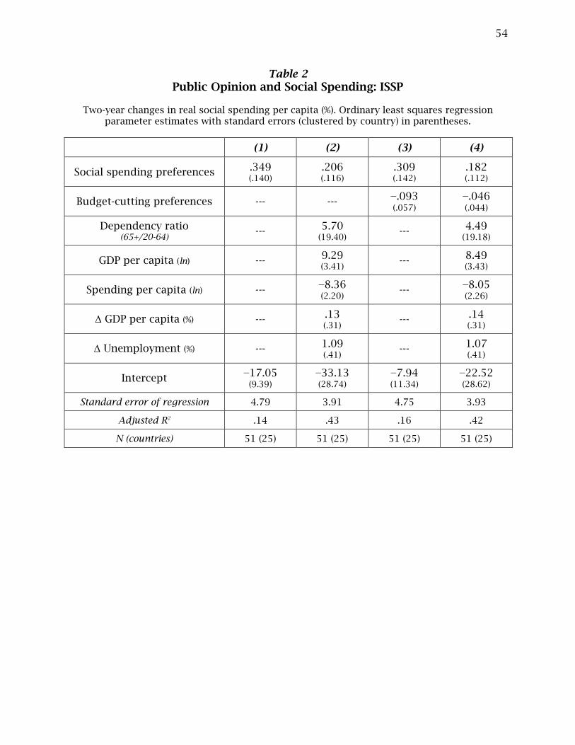
54
Table 2
Public Opinion and Social Spending: ISSP
Two-year changes in real social spending per capita (%). Ordinary least squares regression parameter estimates with standard errors (clustered by country) in parentheses.
(1) (2) (3) (4)
Social spending preferences .349
(.140) .206
(.116) .309
(.142) .182
(.112)
Budget-cutting preferences --- --- −.093
(.057) −.046
(.044)
Dependency ratio (65+/20-64)
--- 5.70
(19.40) --- 4.49
(19.18)
GDP per capita (ln) --- 9.29
(3.41) ---
8.49
(3.43)
Spending per capita (ln) --- −8.36
(2.20) ---
−8.05
(2.26)
Δ GDP per capita (%) --- .13
(.31) --- .14
(.31)
Δ Unemployment (%) --- 1.09
(.41) --- 1.07
(.41)
Intercept −17.05
(9.39) −33.13
(28.74) −7.94
(11.34) −22.52
(28.62)
Standard error of regression 4.79 3.91 4.75 3.93
Adjusted R2 .14 .43 .16 .42
N (countries) 51 (25) 51 (25) 51 (25) 51 (25)

55
Table 3
Welfare State Support and Social Spending: ISSP
Two-year changes in real social spending per capita (%). Ordinary least squares regression parameter estimates with standard errors (clustered by country) in parentheses.
(5) (6) (7) (8)
Welfare state support .033
(.049) .104
(.046) .044
(.052) .099
(.041)
Budget-cutting preferences --- --- −.143
(.066) −.069
(.045)
Dependency ratio (65+/20-64)
--- 2.45
(20.75) --- .58
(19.99)
GDP per capita (ln) --- 11.16
(2.73) ---
10.01
(2.87)
Spending per capita (ln) --- −10.18
(2.15) ---
−9.54
(2.23)
Δ GDP per capita (%) --- .05
(.32) --- .07
(.30)
Δ Unemployment (%) --- 1.08
(.39) --- 1.04
(.40)
Intercept 4.28
(3.18) −28.39
(21.44) 13.41
(4.91) −16.70
(22.17)
Standard error of regression 5.22 3.93 5.06 3.91
Adjusted R2 −.01 .42 .05 .43
N (countries) 51 (25) 51 (25) 51 (25) 51 (25)
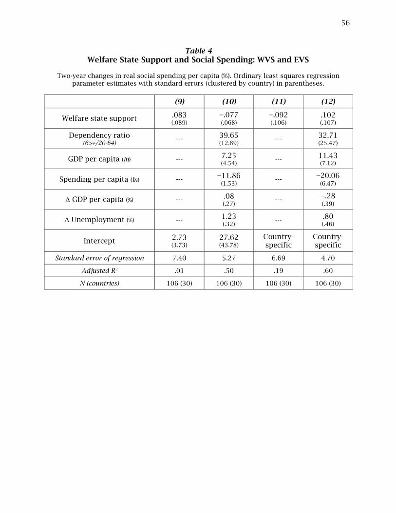
56
Table 4
Welfare State Support and Social Spending: WVS and EVS
Two-year changes in real social spending per capita (%). Ordinary least squares regression parameter estimates with standard errors (clustered by country) in parentheses.
(9) (10) (11) (12)
Welfare state support .083
(.089) −.077
(.068) −.092
(.106) .102
(.107)
Dependency ratio (65+/20-64)
--- 39.65
(12.89) --- 32.71
(25.47)
GDP per capita (ln) --- 7.25
(4.54) --- 11.43
(7.12)
Spending per capita (ln) --- −11.86
(1.53) ---
−20.06
(6.47)
Δ GDP per capita (%) --- .08
(.27) ---
−.28
(.39)
Δ Unemployment (%) --- 1.23
(.32) ---
.80
(.46)
Intercept 2.73
(3.73) 27.62
(43.78) Country-specific
Country-specific
Standard error of regression 7.40 5.27 6.69 4.70
Adjusted R2 .01 .50 .19 .60
N (countries) 106 (30) 106 (30) 106 (30) 106 (30)
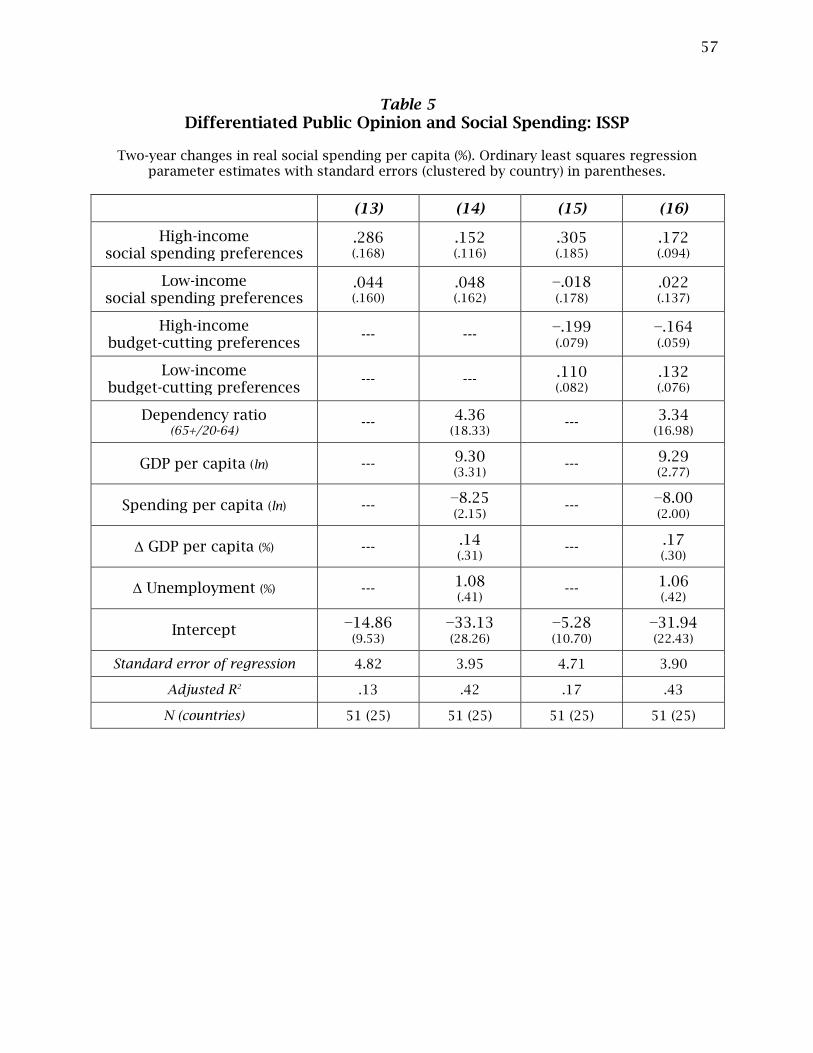
57
Table 5
Differentiated Public Opinion and Social Spending: ISSP
Two-year changes in real social spending per capita (%). Ordinary least squares regression parameter estimates with standard errors (clustered by country) in parentheses.
(13) (14) (15) (16)
High-income social spending preferences
.286
(.168) .152
(.116) .305
(.185) .172
(.094)
Low-income social spending preferences
.044
(.160) .048
(.162) −.018
(.178) .022
(.137)
High-income budget-cutting preferences
--- --- −.199
(.079) −.164
(.059)
Low-income budget-cutting preferences
--- --- .110
(.082) .132
(.076)
Dependency ratio (65+/20-64)
--- 4.36
(18.33) --- 3.34
(16.98)
GDP per capita (ln) --- 9.30
(3.31) ---
9.29
(2.77)
Spending per capita (ln) --- −8.25
(2.15) ---
−8.00
(2.00)
Δ GDP per capita (%) --- .14
(.31) --- .17
(.30)
Δ Unemployment (%) --- 1.08
(.41) --- 1.06
(.42)
Intercept −14.86
(9.53) −33.13
(28.26) −5.28
(10.70) −31.94
(22.43)
Standard error of regression 4.82 3.95 4.71 3.90
Adjusted R2 .13 .42 .17 .43
N (countries) 51 (25) 51 (25) 51 (25) 51 (25)
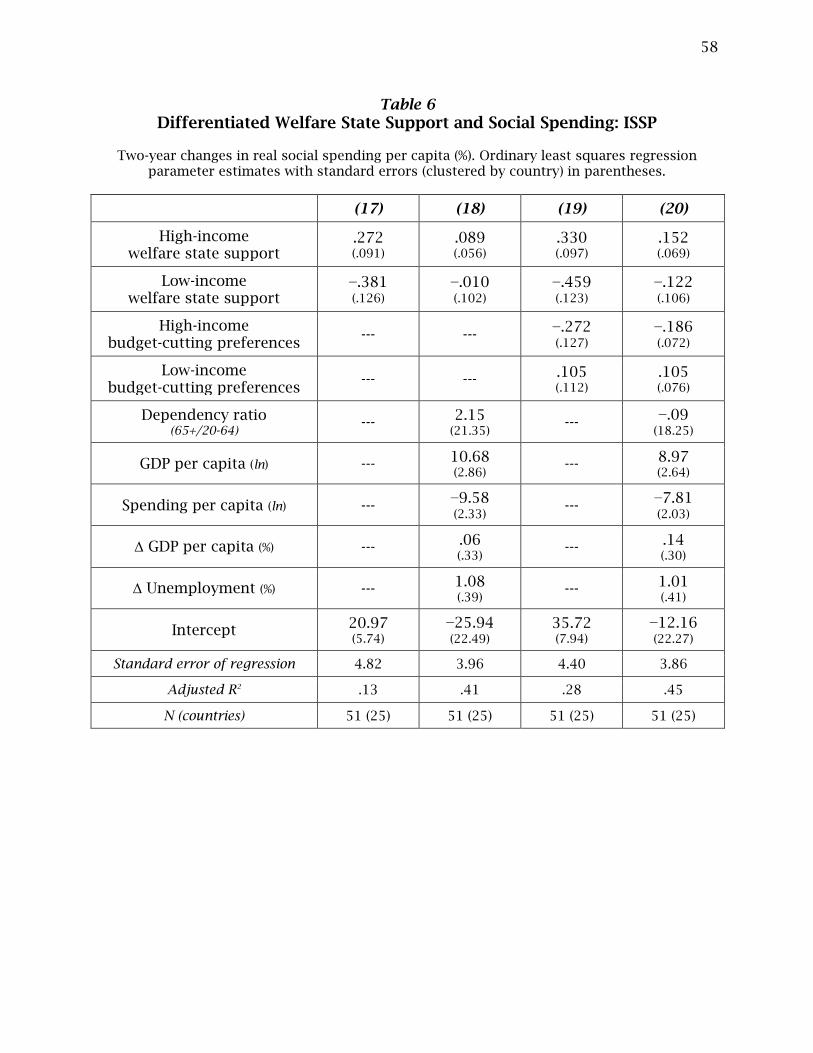
58
Table 6
Differentiated Welfare State Support and Social Spending: ISSP
Two-year changes in real social spending per capita (%). Ordinary least squares regression parameter estimates with standard errors (clustered by country) in parentheses.
(17) (18) (19) (20)
High-income welfare state support
.272
(.091) .089
(.056) .330
(.097) .152
(.069)
Low-income welfare state support
−.381
(.126) −.010
(.102) −.459
(.123) −.122
(.106)
High-income budget-cutting preferences
--- --- −.272
(.127) −.186
(.072)
Low-income budget-cutting preferences
--- --- .105
(.112) .105
(.076)
Dependency ratio (65+/20-64)
--- 2.15
(21.35) ---
−.09
(18.25)
GDP per capita (ln) --- 10.68
(2.86) --- 8.97
(2.64)
Spending per capita (ln) --- −9.58
(2.33) ---
−7.81
(2.03)
Δ GDP per capita (%) --- .06
(.33) --- .14
(.30)
Δ Unemployment (%) --- 1.08
(.39) --- 1.01
(.41)
Intercept 20.97
(5.74) −25.94
(22.49) 35.72
(7.94) −12.16
(22.27)
Standard error of regression 4.82 3.96 4.40 3.86
Adjusted R2 .13 .41 .28 .45
N (countries) 51 (25) 51 (25) 51 (25) 51 (25)

59
Table 7
Differentiated Welfare State Support and Social Spending: WVS and EVS
Two-year changes in real social spending per capita (%). Ordinary least squares regression parameter estimates with standard errors (clustered by country) in parentheses.
(21) (22) (23) (24)
High-income welfare state support
.346
(.172) .127
(.093) .196
(.163) .250
(.133)
Low-income welfare state support
−.265
(.128) −.199
(.063) −.266
(.114) −.135
(.090)
Dependency ratio (65+/20-64)
--- 34.77
(13.74) --- 39.37
(21.25)
GDP per capita (ln) --- 5.52
(4.75) --- 13.87
(7.59)
Spending per capita (ln) --- −10.60
(1.94) ---
−20.96
(6.36)
Δ GDP per capita (%) --- .07
(.27) ---
−.20
(.38)
Δ Unemployment (%) --- 1.20
(.30) --- .90
(.43)
Intercept 6.42
(2.42) 37.44
(43.21) Country-specific
Country-specific
Standard error of regression 7.14 5.19 6.60 4.61
Adjusted R2 .08 .55 .21 .62
N (countries) 106 (30) 106 (30) 106 (30) 106 (30)
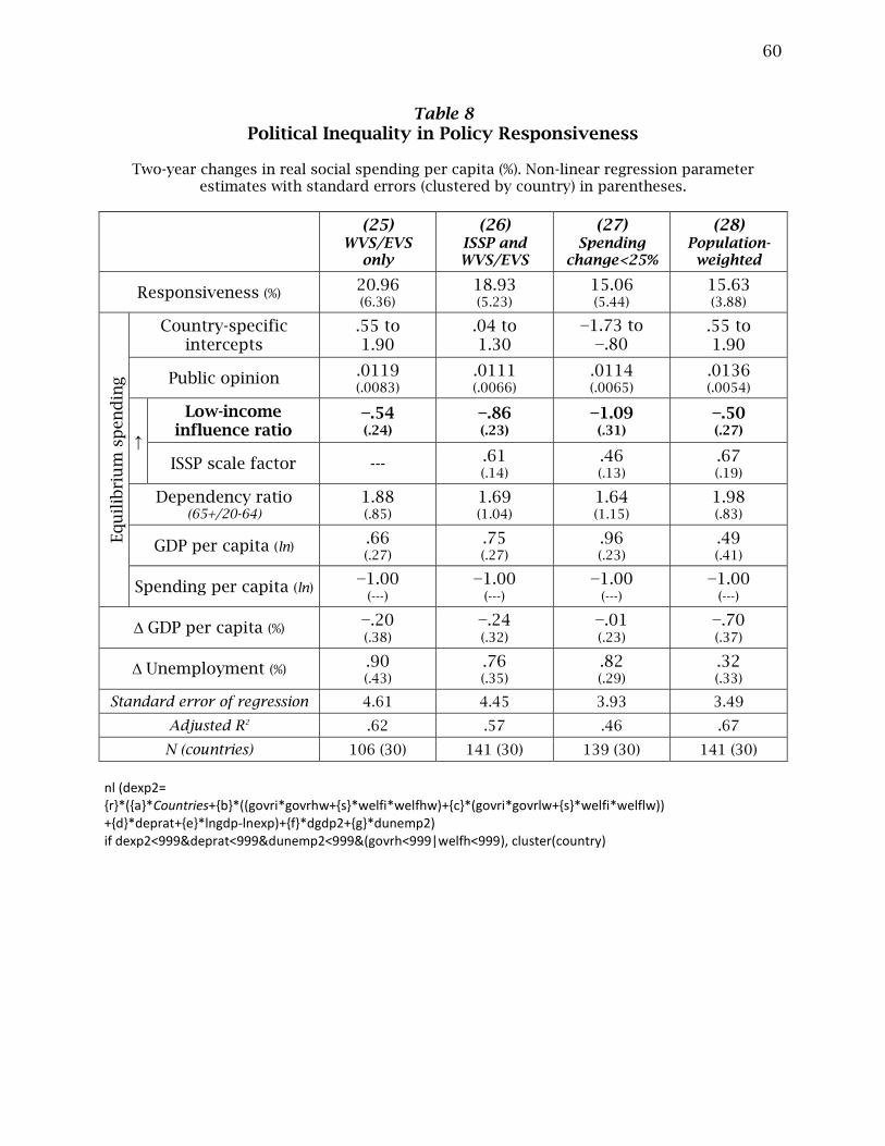
60
Table 8
Political Inequality in Policy Responsiveness
Two-year changes in real social spending per capita (%). Non-linear regression parameter estimates with standard errors (clustered by country) in parentheses.
(25)
WVS/EVS only
(26) ISSP and WVS/EVS
(27) Spending
change<25%
(28) Population-weighted
Responsiveness (%) 20.96
(6.36) 18.93
(5.23) 15.06
(5.44) 15.63
(3.88)
Eq
uil
ibri
um
sp
en
din
g
Country-specific intercepts
.55 to 1.90
.04 to 1.30
−1.73 to −.80
.55 to 1.90
Public opinion .0119
(.0083) .0111
(.0066) .0114
(.0065) .0136
(.0054)
↑
Low-income influence ratio
−.54 (.24)
−.86 (.23)
−1.09 (.31)
−.50 (.27)
ISSP scale factor --- .61 (.14)
.46 (.13)
.67 (.19)
Dependency ratio (65+/20-64)
1.88
(.85) 1.69
(1.04)
1.64
(1.15) 1.98 (.83)
GDP per capita (ln) .66 (.27)
.75 (.27)
.96 (.23)
.49
(.41)
Spending per capita (ln) −1.00
(---) −1.00
(---) −1.00
(---) −1.00
(---)
Δ GDP per capita (%) −.20
(.38) −.24
(.32) −.01
(.23) −.70
(.37)
Δ Unemployment (%) .90
(.43) .76
(.35) .82
(.29) .32
(.33)
Standard error of regression 4.61 4.45 3.93 3.49
Adjusted R2 .62 .57 .46 .67
N (countries) 106 (30) 141 (30) 139 (30) 141 (30)
nl (dexp2= {r}*({a}*Countries+{b}*((govri*govrhw+{s}*welfi*welfhw)+{c}*(govri*govrlw+{s}*welfi*welflw)) +{d}*deprat+{e}*lngdp-lnexp)+{f}*dgdp2+{g}*dunemp2) if dexp2<999&deprat<999&dunemp2<999&(govrh<999|welfh<999), cluster(country)
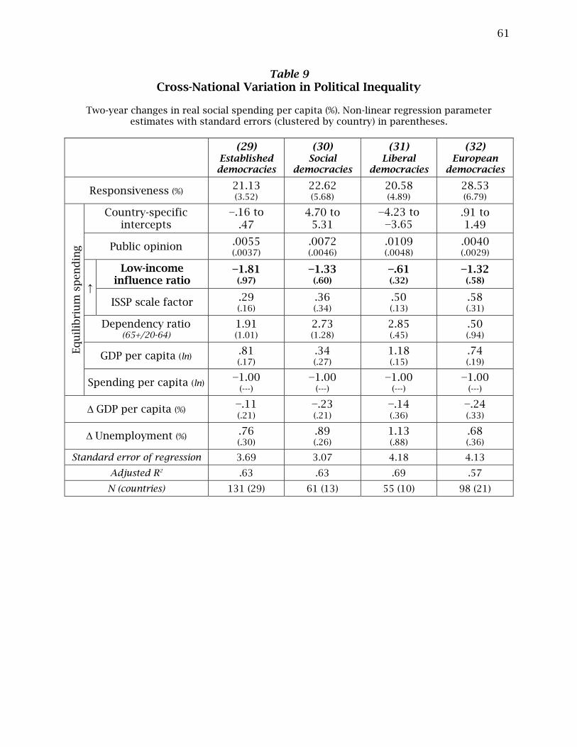
61
Table 9
Cross-National Variation in Political Inequality
Two-year changes in real social spending per capita (%). Non-linear regression parameter estimates with standard errors (clustered by country) in parentheses.
(29)
Established democracies
(30) Social
democracies
(31) Liberal
democracies
(32) European
democracies
Responsiveness (%) 21.13
(3.52) 22.62
(5.68) 20.58
(4.89) 28.53
(6.79)
Eq
uil
ibri
um
sp
en
din
g
Country-specific intercepts
−.16 to .47
4.70 to 5.31
−4.23 to −3.65
.91 to 1.49
Public opinion .0055
(.0037)
.0072
(.0046) .0109
(.0048)
.0040
(.0029)
↑
Low-income influence ratio
−1.81 (.97)
−1.33 (.60)
−.61 (.32)
−1.32 (.58)
ISSP scale factor .29 (.16)
.36 (.34)
.50 (.13)
.58 (.31)
Dependency ratio (65+/20-64)
1.91
(1.01)
2.73
(1.28) 2.85
(.45)
.50
(.94)
GDP per capita (ln) .81 (.17)
.34 (.27)
1.18 (.15)
.74 (.19)
Spending per capita (ln) −1.00
(---)
−1.00
(---) −1.00
(---)
−1.00
(---)
Δ GDP per capita (%) −.11
(.21) −.23
(.21) −.14
(.36) −.24
(.33)
Δ Unemployment (%) .76
(.30) .89
(.26) 1.13
(.88) .68
(.36)
Standard error of regression 3.69 3.07 4.18 4.13
Adjusted R2 .63 .63 .69 .57
N (countries) 131 (29) 61 (13) 55 (10) 98 (21)

62
Table 10
Political Institutions and Political Inequality
Two-year changes in real social spending per capita (%). Non-linear regression parameter estimates with standard errors (clustered by country) in parentheses.
(33)
Federal (34)
Centralized (35)
Proportional (36)
Plurality
Responsiveness (%) 20.84
(10.73) 22.35
(7.51) 29.09
(8.55) 17.46
(6.45)
Eq
uil
ibri
um
sp
en
din
g
Country-specific intercepts
−5.75 to −4.70
.23 to 1.24
.85 to 1.50
−5.36 to −4.65
Public opinion −.0024
(.0029) .0136
(.0073) .0038
(.0028)
.0140
(.0047)
↑
Low-income influence ratio
−.19 (.34)
−.83 (.21)
−1.57 (.92)
−.46 (.31)
ISSP scale factor 1.29 (1.73)
.61 (.18)
.55 (.32)
.43 (.15)
Dependency ratio (65+/20-64)
−.62
(.56)
2.42
(1.07) .48
(1.01)
2.89
(.46)
GDP per capita (ln) 1.36 (.18)
.74 (.34)
.74 (.19)
1.29 (.28)
Spending per capita (ln) −1.00
(---) −1.00
(---) −1.00
(---)
−1.00
(---)
Δ GDP per capita (%) .36
(.41) −.39
(.44) −.23
(.35) .22
(.42)
Δ Unemployment (%) .97
(.35) .61
(.60) .69
(.37) 2.10
(.89)
Standard error of regression 3.35 5.16 4.41 3.73
Adjusted R2 .30 .62 .56 .71
N (countries) 64 (13) 77 (18) 86 (20) 55 (11)

63
Table 11
Economic Development and Political Inequality
Two-year changes in real social spending per capita (%). Non-linear regression parameter estimates with standard errors (clustered by country) in parentheses.
(37)
GDP/capita > $30,000
(38) GDP/capita < $30,000
(39) Post-transfer
Gini > 30
(40) Post-transfer
Gini < 30
Responsiveness (%) 17.62
(7.11) 17.36
(11.41) 24.24
(3.87) 15.62
(15.81)
Eq
uil
ibri
um
sp
en
din
g
Intercept 6.34 to
7.30 −5.46 to
−3.17 −4.03 to
−2.95 5.67 to
6.83
Public opinion .0084
(.0043) .0113
(.0110) .0115
(.0053)
.0099
(.0104)
↑
Low-income influence ratio
−.62 (.34)
−.85 (.40)
−.77 (.23)
−1.10 (.71)
ISSP scale factor .68 (.43)
.85 (.53)
.46 (.11)
.56 (.32)
Dependency ratio
(65+/20-64) 3.33
(1.30)
−7.99
(11.07) 1.38
(1.02)
2.54
(2.36)
GDP per capita (ln) .15 (.44)
1.43 (.83)
1.17 (.16)
.23 (.57)
Spending per capita (ln) −1.00
(---) −1.00
(---) −1.00
(---)
−1.00
(---)
Δ GDP per capita (%) −.24
(.31) −.24
(.70) −.27
(.20) −.01
(.41)
Δ Unemployment (%) 1.10
(.66) .92
(1.04) .51
(.27) 1.22
(.67)
Standard error of regression 3.15 6.11 3.83 4.75
Adjusted R2 .47 .51 .69 .46
N (countries) 79 (21) 62 (21) 70 (17) 71 (20)

64
Table A1
Country-Years
Survey data from International Social Survey Programme and World Values Surveys and European Values Surveys (*combined) merged with OECD Social Expenditures data, 1985-2015.
Australia (AU) 1986, 1990, 1997, 2007 1995, 2005, 2012
Austria (AT) --- 1990, 1999, 2008
Belgium (BE) --- 1990, 1999, 2009
Canada (CA) 1996, 2006 2000, 2006
Chile (CL) 2006 1996, 2000, 2006, 2011
Czech Republic (CZ) 1996, 2006 1991*, 1998, 1999, 2008
Denmark (DK) 2008 1990, 1999, 2008
Estonia (EE) --- 2011
Finland (FI) 2006 1990, 1996, 2000, 2005, 2009
France (FR) 1997, 2006 1990, 1999, 2006, 2008
Germany (DE) 1985, 1990, 1996, 2006 1990, 1997, 1999, 2006, 2008
Great Britain (GB) 1985, 1990, 1996, 2006 1990, 1999, 2005, 2009
Hungary (HU) 2006 1999, 2008, 2009
Iceland (IS) --- 1999, 2009
Ireland (IE) (1991), 1996, 2006 1990, 1999, 2008
Israel (IL) 2007 2001
Italy (IT) 1985, 1990, 1996 1990, 1999, 2005, 2009
Japan (JP) 1996, 2006 1990, 1995, 2000, 2005, 2010
Mexico (MX) --- 2000, 2005
Netherlands (NL) 2006 1990, 1999, 2006, 2008
New Zealand (NZ) 1997, 2006 1998, 2004, 2011
Norway (NO) 1990, 1996, 2006 1996, 2007
Poland (PL) 1997, 2008 1990, 1997, 1999, 2005, 2008
Portugal (PT) 2006 1990, 1999, 2008
Slovenia (SI) 2006 1999, 2005, 2008, 2011
South Korea (KR) 2006 1990, 1996, 2001, 2005, 2010
Spain (ES) 1996, 2007 1990*, 1995, 1999, 2000, 2007, 2008, 2011
Sweden (SE) 1996, 2006 1990, 1996, 1999, 2006, 2009, 2011
Switzerland (CH) 1998, 2007 1996, 2007
United States (US) 1985, 1990, 1996, 2006 1995, 1999, 2006, 2011
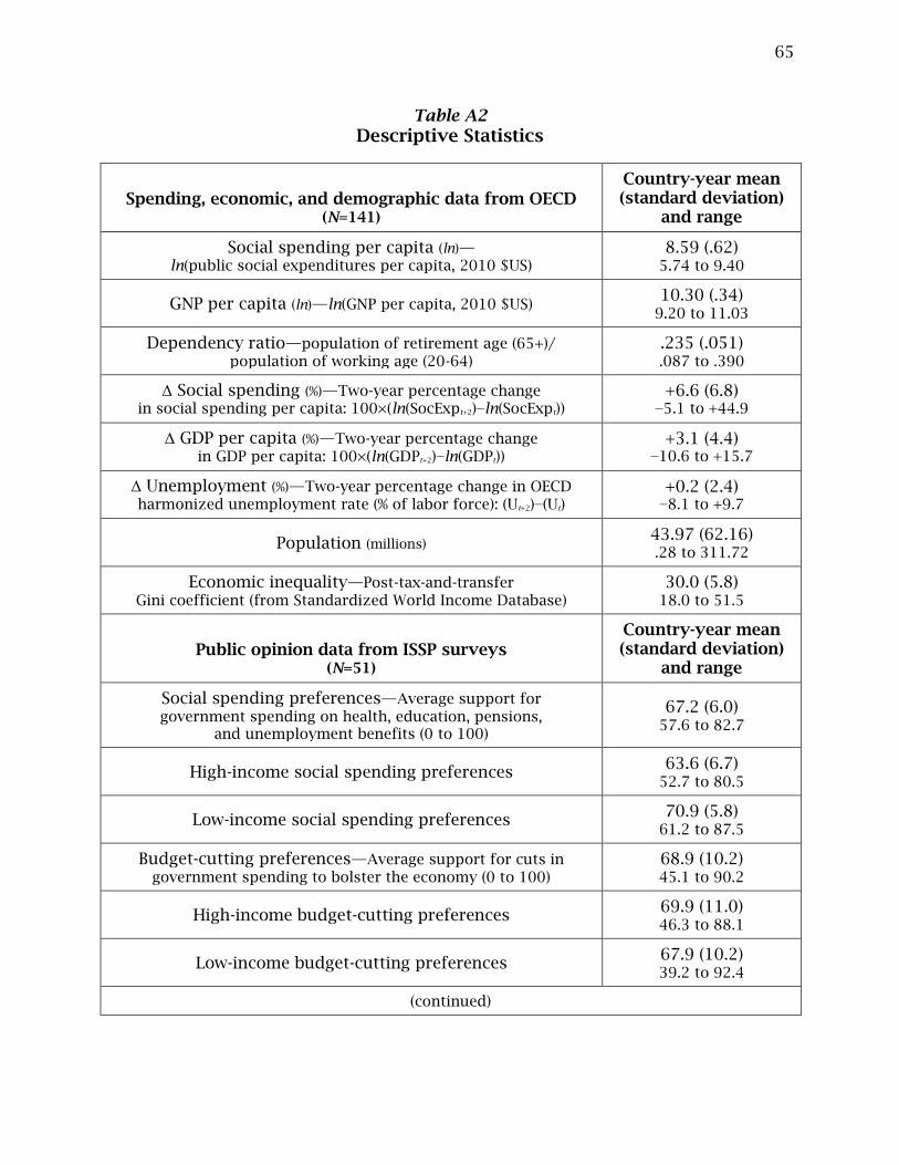
65
Table A2
Descriptive Statistics
Spending, economic, and demographic data from OECD
(N=141)
Country-year mean (standard deviation)
and range
Social spending per capita (ln)— ln(public social expenditures per capita, 2010 $US)
8.59 (.62) 5.74 to 9.40
GNP per capita (ln)—ln(GNP per capita, 2010 $US) 10.30 (.34)
9.20 to 11.03
Dependency ratio—population of retirement age (65+)/ population of working age (20-64)
.235 (.051) .087 to .390
Δ Social spending (%)—Two-year percentage change in social spending per capita: 100×(ln(SocExpt+2)−ln(SocExpt))
+6.6 (6.8) −5.1 to +44.9
Δ GDP per capita (%)—Two-year percentage change in GDP per capita: 100×(ln(GDPt+2)−ln(GDPt))
+3.1 (4.4) −10.6 to +15.7
Δ Unemployment (%)—Two-year percentage change in OECD harmonized unemployment rate (% of labor force): (Ut+2)−(Ut)
+0.2 (2.4) −8.1 to +9.7
Population (millions) 43.97 (62.16) .28 to 311.72
Economic inequality—Post-tax-and-transfer Gini coefficient (from Standardized World Income Database)
30.0 (5.8) 18.0 to 51.5
Public opinion data from ISSP surveys
(N=51)
Country-year mean (standard deviation)
and range
Social spending preferences—Average support for government spending on health, education, pensions,
and unemployment benefits (0 to 100)
67.2 (6.0) 57.6 to 82.7
High-income social spending preferences 63.6 (6.7)
52.7 to 80.5
Low-income social spending preferences 70.9 (5.8)
61.2 to 87.5
Budget-cutting preferences—Average support for cuts in government spending to bolster the economy (0 to 100)
68.9 (10.2) 45.1 to 90.2
High-income budget-cutting preferences 69.9 (11.0) 46.3 to 88.1
Low-income budget-cutting preferences 67.9 (10.2) 39.2 to 92.4
(continued)
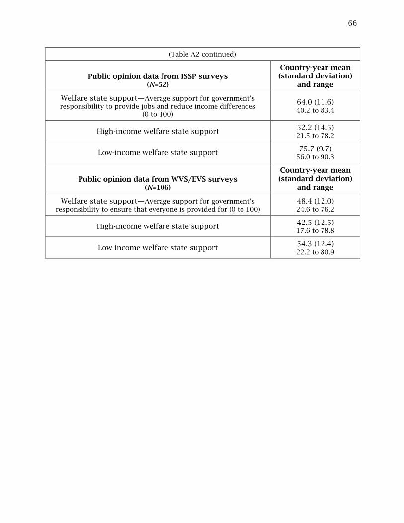
66
(Table A2 continued)
Public opinion data from ISSP surveys
(N=52)
Country-year mean (standard deviation)
and range
Welfare state support—Average support for government’s responsibility to provide jobs and reduce income differences
(0 to 100)
64.0 (11.6) 40.2 to 83.4
High-income welfare state support 52.2 (14.5) 21.5 to 78.2
Low-income welfare state support 75.7 (9.7)
56.0 to 90.3
Public opinion data from WVS/EVS surveys
(N=106)
Country-year mean (standard deviation)
and range
Welfare state support—Average support for government’s responsibility to ensure that everyone is provided for (0 to 100)
48.4 (12.0) 24.6 to 76.2
High-income welfare state support 42.5 (12.5) 17.6 to 78.8
Low-income welfare state support 54.3 (12.4) 22.2 to 80.9
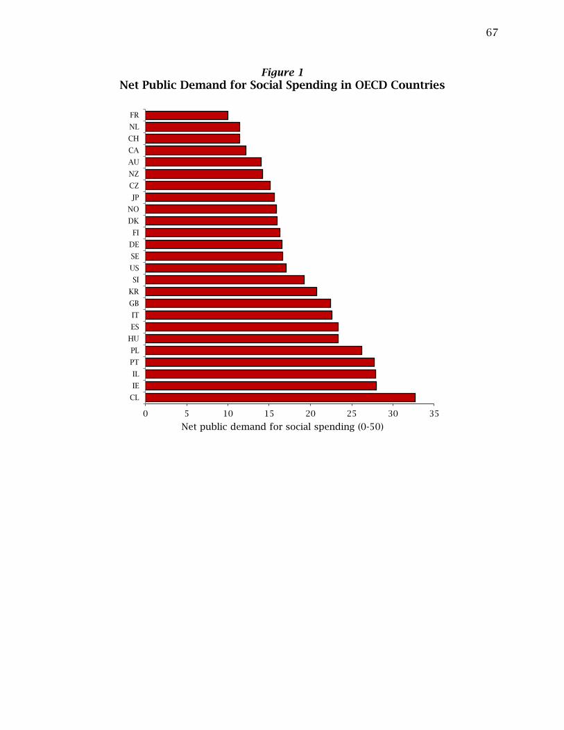
67
Figure 1
Net Public Demand for Social Spending in OECD Countries
0 5 10 15 20 25 30 35
CL
IE
IL
PT
PL
HU
ES
IT
GB
KR
SI
US
SE
DE
FI
DK
NO
JP
CZ
NZ
AU
CA
CH
NL
FR
Net public demand for social spending (0-50)
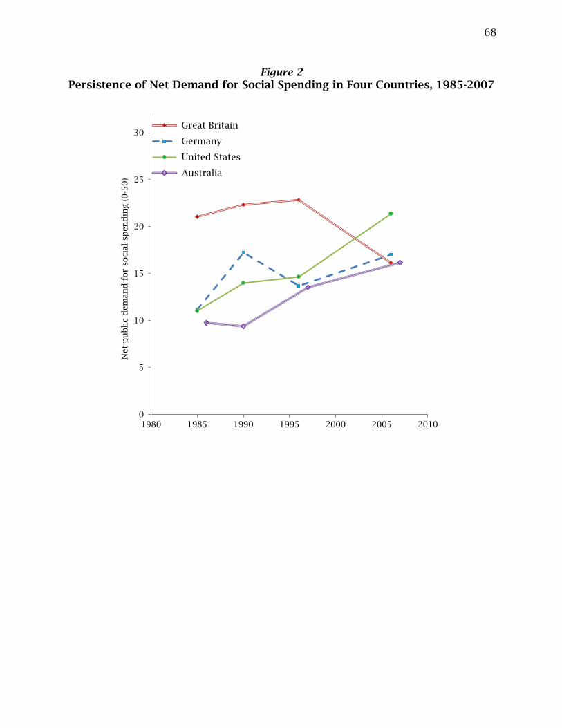
68
Figure 2
Persistence of Net Demand for Social Spending in Four Countries, 1985-2007
0
5
10
15
20
25
30
1980 1985 1990 1995 2000 2005 2010
Net
pu
bli
c d
em
an
d f
or
socia
l sp
en
din
g (
0-5
0)
Great Britain
Germany
United States
Australia

69
Figure 3
Social Spending Preferences and Policy Change
AU86
AU90
AU97
AU07
CA96
CA06
CL06
CZ96
CZ06
DK08
FI06
FR97
FR06
DE85 DE90
DE96DE06
HU06IE96
IE06
IL07
IT85IT90IT96
JP96
JP06
KR06
NL06
NZ97NZ06
NO90
NO96
NO06
PL97PL08
PT06SI06ES96
ES07
SE96
SE06
CH98
CH07
GB85
GB90
GB96
GB06
US85
US90
US96
US06
-50
51
01
52
0
Tw
o-y
ear
ch
an
ge i
n s
ocia
l sp
en
din
g (
%)
0 5 10 15 20 25 30 35
Net public demand for social spending (0-50)
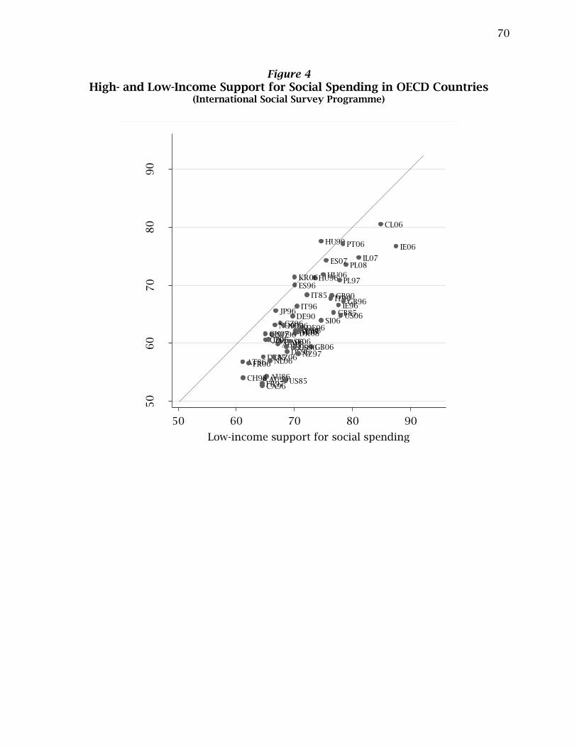
70
Figure 4
High- and Low-Income Support for Social Spending in OECD Countries (International Social Survey Programme)
AU86AU90
AU97
AU07
AT86
CA96
CA06
CL06
CZ96
CZ06DK08FI06
FR97
FR06DE85
DE90
DE96
DE06
HU90
HU96HU06
IE96
IE06
IL07
IT85 IT90IT96
JP96
JP06
KR06
NL06NZ97NZ06
NO90NO96
NO06
PL97
PL08
PT06
SI06
ES96
ES07
SE96
SE06
CH98
CH07
GB85
GB90GB96
GB06
US85
US90US96
US06
50
60
70
80
90
Hig
h-i
ncom
e s
up
po
rt f
or
socia
l sp
en
din
g
50 60 70 80 90
Low-income support for social spending
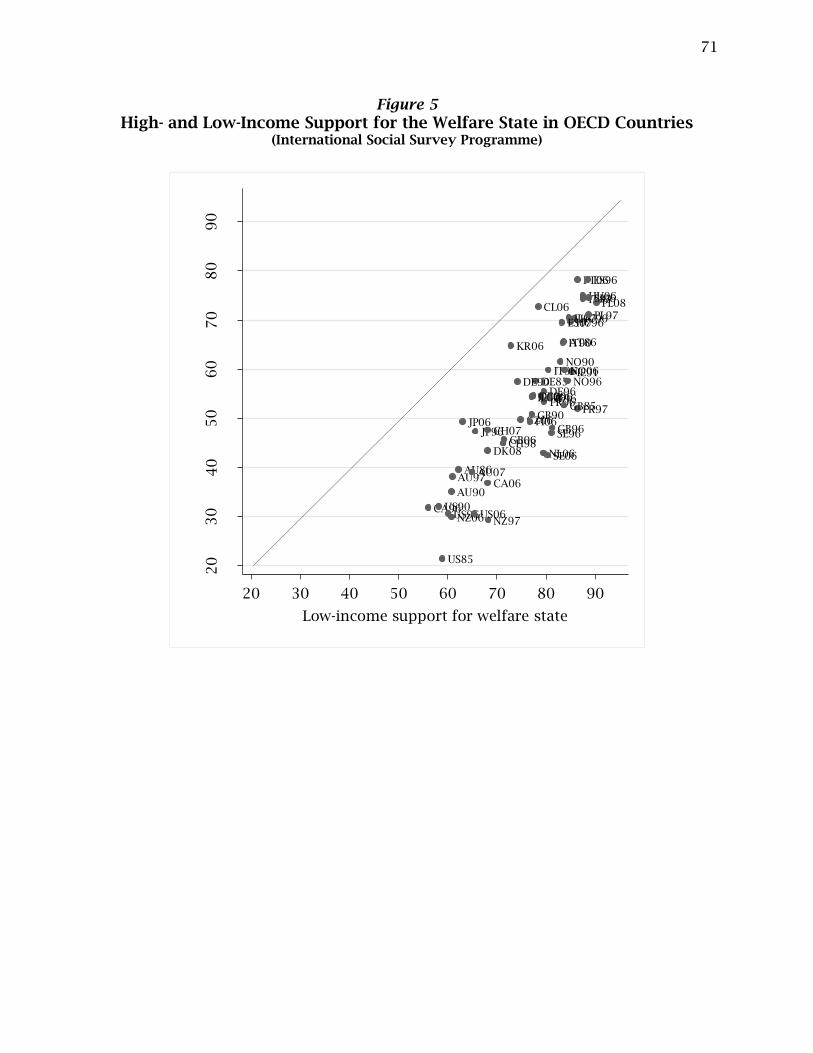
71
Figure 5
High- and Low-Income Support for the Welfare State in OECD Countries (International Social Survey Programme)
AU86
AU90
AU97AU07
AT86
CA96
CA06
CL06
CZ96
CZ06
DK08
FI06FR97
FR06
DE85DE90DE96DE06
HU90HU96
HU06
IE91
IE96IE06
IL07
IT85
IT90
IT96
JP96JP06
KR06
NL06
NZ97NZ06
NO90
NO96NO06
PL97PL08
PT06
SI06
ES96
ES07
SE96
SE06CH98
CH07
GB85GB90
GB96GB06
US85
US90US96US06
20
30
40
50
60
70
80
90
Hig
h-i
ncom
e s
up
po
rt f
or
welf
are
sta
te
20 30 40 50 60 70 80 90
Low-income support for welfare state
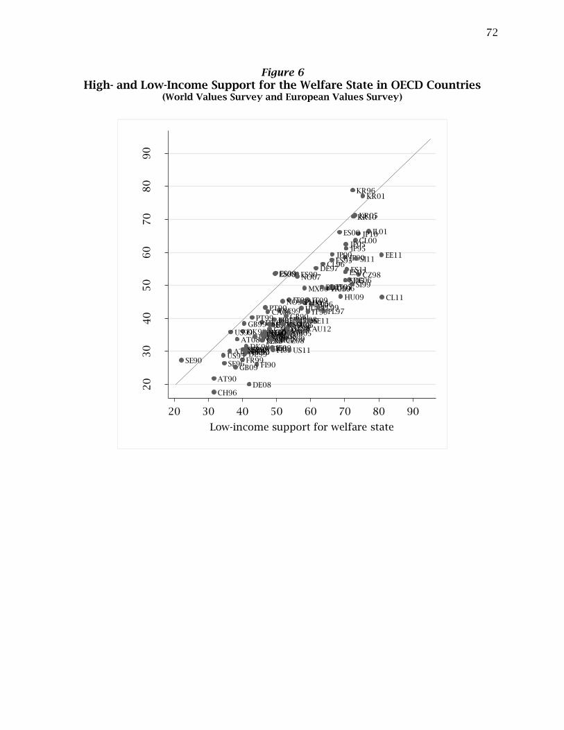
72
Figure 6
High- and Low-Income Support for the Welfare State in OECD Countries (World Values Survey and European Values Survey)
AU95AU05
AU12
AT90
AT99
AT08
BE90
BE99
BE09
CA00
CA06
CL96
CL00
CL06
CL11
CZ91
CZ98
CZ99CZ08
DK90
DK99
DK08
EE11
FI90
FI96
FI00
FI05
FI09FR90FR99
FR06FR08
DE90
DE97
DE99
DE06
DE08
HU99
HU08
HU09
IS99 IS09
IE90
IE99
IE08
IL01
IT90
IT99
IT05
IT09
JP90
JP95JP00
JP05
JP10
KR90
KR96KR01
KR05KR10
MX00
MX05
NL90NL99
NL06
NL08NZ98
NZ04NZ11
NO96
NO07
PL90
PL97PL99
PL05
PL08
PT90
PT99
PT08
SI99SI05
SI08
SI11
ES90
ES95
ES99
ES00
ES07ES08ES11
SE90 SE96
SE99SE06
SE09
SE11
CH96
CH07
GB90GB99
GB05
GB09
US95
US99US06
US11
20
30
40
50
60
70
80
90
Hig
h-i
ncom
e s
up
po
rt f
or
welf
are
sta
te
20 30 40 50 60 70 80 90
Low-income support for welfare state
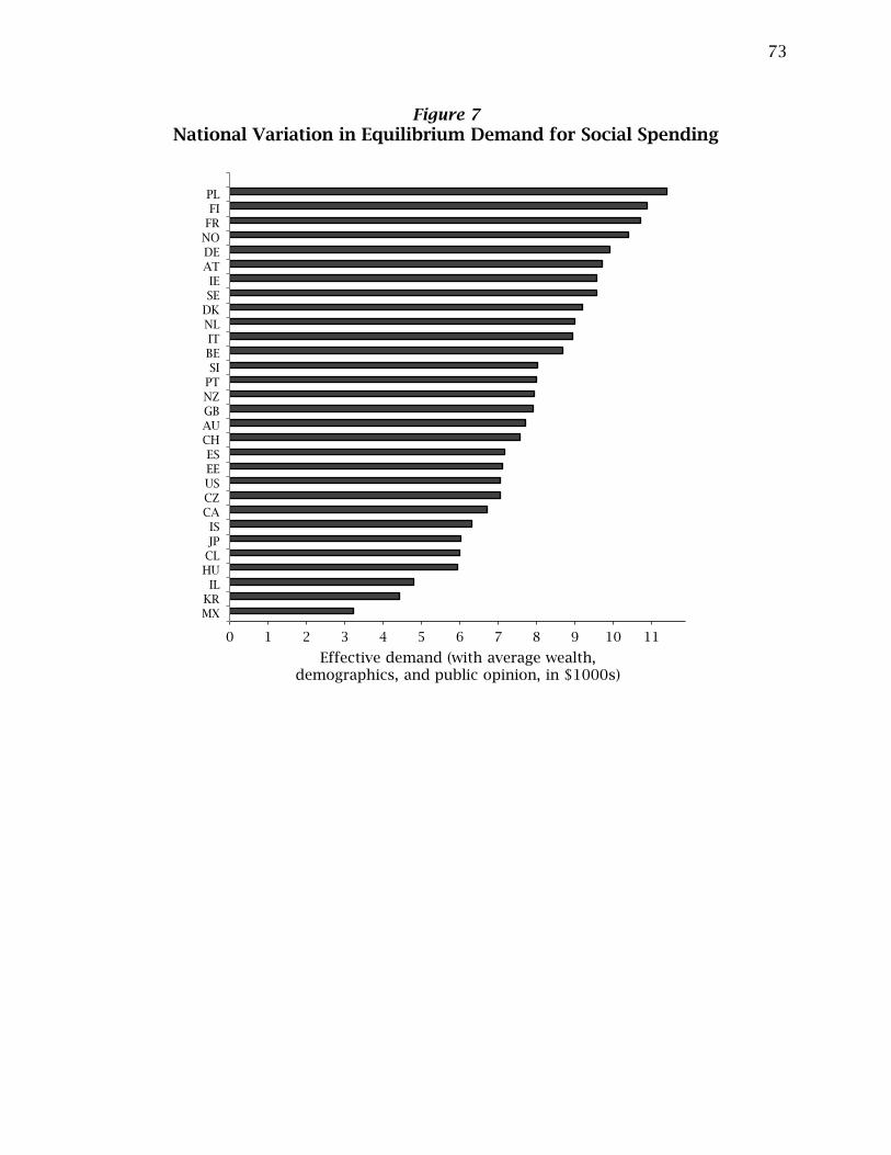
73
Figure 7
National Variation in Equilibrium Demand for Social Spending
0 1 2 3 4 5 6 7 8 9 10 11
MX
KR
IL
HU
CL
JP
IS
CA
CZ
US
EE
ES
CH
AU
GB
NZ
PT
SI
BE
IT
NL
DK
SE
IE
AT
DE
NO
FR
FI
PL
Effective demand (with average wealth,demographics, and public opinion, in $1000s)

74
Figure 8
Estimated Reduction in Effective Demand for Social Spending Due to Biased Responsiveness to Public Opinion
0 5 10 15 20
EE
NZ
CZ
SI
AU
FI
IS
CL
HU
PL
US
FR
GB
CH
NL
IE
DE
IT
CA
MX
SE
NO
BE
IL
JP
DK
AT
PT
ES
KR
Reduction in effective demand (%)