POLITECNICO DI MILANO

Facoltà di Ingegneria IndustrialeCorso di laurea in Ingegneria Aeronautica

RESIDUAL BASED DISCRETIZATION OF

MADSEN AND SØRENSEN SYSTEM OF

BOUSSINESQ EQUATIONS FOR

NON-HYDROSTATIC WAVE

PROPAGATION

Relatore:

Prof. Alberto Matteo Attilio GUARDONE

Correlatore:

Prof. Mario RICCHIUTO

Tesi di Laurea di

Andrea Gilberto FILIPPINI

Matr. 762975

Anno Accademico 2011-2012

Contents

Abstract ix

Sommario xi

Introduction 1

1 Governing Equations 7

1.1 Nonlinear Shallow Water Equations (NSWE) . . . . . . . . . . 7

1.2 Madsen and Sørensen Boussinesq-type Equations . . . . . . . 10

1.3 Model Dispersion Analysis . . . . . . . . . . . . . . . . . . . . 15

2 Weighted Residuals Methods 23

3 Linear Scalar Advection Equation 29

3.1 Finite Dierence Methods . . . . . . . . . . . . . . . . . . . . 30

3.2 Galerkin Finite Element Method . . . . . . . . . . . . . . . . 34

3.3 Residual Distribution Method . . . . . . . . . . . . . . . . . . 39

3.4 Stabilized Upwind Methods . . . . . . . . . . . . . . . . . . . 43

3.5 Conclusions . . . . . . . . . . . . . . . . . . . . . . . . . . . . 51

i

4 Linear Scalar Advection with Dispersion Equation 53

4.1 Finite Dierence Methods . . . . . . . . . . . . . . . . . . . . 54

4.2 Galerkin nite element method . . . . . . . . . . . . . . . . . 57

4.3 Residual distribution method . . . . . . . . . . . . . . . . . . 59

4.4 Stabilized Upwind methods . . . . . . . . . . . . . . . . . . . 64

4.5 Conclusions . . . . . . . . . . . . . . . . . . . . . . . . . . . . 70

5 Madsen and Sørensen system discretisation 73

5.1 Finite dierence methods . . . . . . . . . . . . . . . . . . . . . 74

5.2 Galerkin nite element method . . . . . . . . . . . . . . . . . 79

5.3 Residual Distribution . . . . . . . . . . . . . . . . . . . . . . . 85

5.4 Stabilized Upwind methods . . . . . . . . . . . . . . . . . . . 90

5.5 Conclusions . . . . . . . . . . . . . . . . . . . . . . . . . . . . 98

6 Time discretization 101

6.1 Crank-Nicolson time integration method . . . . . . . . . . . . 103

6.2 BDF3 time integration method . . . . . . . . . . . . . . . . . 110

7 Numerical implementation 113

7.1 Soliton Wave Generator . . . . . . . . . . . . . . . . . . . . . 114

7.2 Boundary conditions . . . . . . . . . . . . . . . . . . . . . . . 119

7.3 Internal Wave Generation . . . . . . . . . . . . . . . . . . . . 121

8 Numerical Tests and Results 125

8.1 Convergence Analysis . . . . . . . . . . . . . . . . . . . . . . . 125

ii

8.2 Head-on Collision of Two Solitary Waves . . . . . . . . . . . . 130

8.3 Propagation over a Shelf . . . . . . . . . . . . . . . . . . . . . 134

8.4 Periodic Wave Propagation over a Submerged Bar . . . . . . . 139

Conclusions 143

A Demonstration of the Equality 2.5 149

B Auxiliary Variables Choice for the Linear Advection-Dispersion

Problem 151

C Space-Discretization of the Linearized MS System 155

D Auxiliary Variables Choice in the MS Dispersion Term Dis-

cretization 159

E Galerkin Space-Discretization of the MS System 161

F Space-Time Discretization of the Linearized MS System 163

Bibliography 165

iii

iv

List of Figures

1.1 Schematic representation of the advection and convergencecontribution in equation (1.2). In the gure H is assume tolocally increase.) . . . . . . . . . . . . . . . . . . . . . . . . . 8

1.2 Sketch of the free surface ow problem, main parameters de-scription. . . . . . . . . . . . . . . . . . . . . . . . . . . . . . . 11

1.3 Free surface time history illustrating a soliton wave propaga-tion over a bed variation (g); comparison between the solutionscomputed by means of NSWE (left) and MS (right) models. . 13

1.4 Free surface time history illustrating a soliton wave propaga-tion over a bed variation (g); comparison between the solutionscomputed by means of NSWE (left) and MS (right) models. . 14

1.5 Comparison of the dispersion characteristics of the Peregrine'sBoussinesq, extended Boussinesq and shallow water modelswith respect to the linear wave theory, based on the represen-tation of the percentage of error in phase velocity computation. 20

2.1 Representation of the linear nite basis function at the node i. 25

3.1 Dispersion w against the wavenumber k of the nite dier-ence schemes FD2 and FD4, compared to the scalar linearadvection model one, when the wavelength is discretized witha number of grid nodes N = 5. . . . . . . . . . . . . . . . . . . 34

3.2 Representation of the linear nite basis function over the ele-ment e. . . . . . . . . . . . . . . . . . . . . . . . . . . . . . . . 35

v

3.3 Dispersion w against the wavenumber k of the Galerkin niteelement scheme, compared to the scalar linear advection modeland to the previous mentioned schemes, when the wavelengthis discretized with a number of grid nodes N = 5. . . . . . . . 38

3.4 Dispersion w against the wavenumber k of the central RDscheme, compared to the scalar linear advection model andto the previous mentioned schemes, when the wavelength isdiscretized with a number of grid nodes N = 5. . . . . . . . . 43

3.5 Representation of the upwind linear nite basis function overthe element e. . . . . . . . . . . . . . . . . . . . . . . . . . . . 46

3.6 Dispersion w against the wavenumber k of the stabilized up-wind schemes, compared to the scalar linear advection modeland to the previous mentioned schemes, when the wavelengthis discretized with a number of grid nodes N = 5. . . . . . . . 50

3.7 Diusion ξ against the wavenumber k of the stabilized upwindSU/PG and U/RD schemes, compared to the scalar linearadvection model, when the wavelength is discretized with anumber of grid nodes N = 5. . . . . . . . . . . . . . . . . . . . 50

4.1 Dispersion w against the wavenumber k of the nite dierenceFD2 and FD4 schemes, compared to the scalar linear advec-tion with dispersion model, when the wavelength is discretizedwith a number of grid nodes N = 5. . . . . . . . . . . . . . . . 56

4.2 Dispersion w against the wavenumber k of the Galerkin -nite element scheme, compared to the scalar linear advectionwith dispersion model and to the previous mentioned schemes,when the wavelength is discretized with a number of grid nodesN = 5. . . . . . . . . . . . . . . . . . . . . . . . . . . . . . . . 59

4.3 Dispersion w against the wavenumber k of the central RDscheme, compared to the scalar linear advection with disper-sion model and to the previous mentioned schemes, when thewavelength is discretized with a number of grid nodes N = 5. . 63

vi

4.4 Dispersion w against the wavenumber k of the stabilized up-wind SU/PG and U/RD schemes, compared to the scalarlinear advection with dispersion model and to the previousmentioned schemes, when the wavelength is discretized witha number of grid nodes N = 5. . . . . . . . . . . . . . . . . . . 69

4.5 Diusion ξ against the wavenumber k of the stabilized up-wind SU/PG and U/RD schemes, compared to the scalarlinear advection with dispersion model, when the wavelengthis discretized with a number of grid nodes N = 5. . . . . . . . 70

5.1 Dispersion w against the wavenumber k of the nite dierenceFD2 and FD4 schemes, compared to Airy theory value (1.25),when the wavelength is discretized with a number of grid nodesN = 5. . . . . . . . . . . . . . . . . . . . . . . . . . . . . . . . 78

5.2 Dispersion w against the wavenumber k of the Galerkin niteelement scheme, compared to Airy theory value and to the pre-vious mentioned schemes, when the wavelength is discretizedwith a number of grid nodes N = 5. . . . . . . . . . . . . . . . 84

5.3 Dispersion w against the wavenumber k of the central RDscheme, compared to Airy theory value and to the previousmentioned schemes, when the wavelength is discretized witha number of grid nodes N = 5. . . . . . . . . . . . . . . . . . . 89

5.4 Dispersion w against the wavenumber k of the stabilized up-wind SU/PG and U/RD schemes, compared to Airy theoryvalue and to the previous mentioned schemes, when the wave-length is discretized with a number of grid nodes N = 5. . . . 97

5.5 Diusion ξ against the wavenumber k of the stabilized upwindSU/PG and U/RD schemes, compared to Airy theory valueand to the previous mentioned schemes, when the wavelengthis discretized with a number of grid nodes N = 5. . . . . . . . 97

7.1 Numerical solution of the integration of the second order dif-ferential equation of q using the Matlab R© solver ode113. . . . . 116

vii

7.2 (a): attempts of reconstruction of the tail of the soliton shapeby means of the numerical integration of the rst order equa-tion (7.7); (b): close-up of the interest region. . . . . . . . . . 117

7.3 Optimal solution found for the soliton tail reconstruction andcomparison between the nal and the initial conguration (a);close-up of the interest region (b). . . . . . . . . . . . . . . . . 118

7.4 (a): evolution of the exact a = 0.2 m solitary wave; (b): com-parison between the exact and the numerically computed soli-tary wave plotted against the spatial domain at the nal timeof the simulation. . . . . . . . . . . . . . . . . . . . . . . . . . 119

7.5 sketch of the internal wave generation process. . . . . . . . . . 122

8.1 Spatial distribution of the error function eη(x) over the do-main, parametrised on the growing number of nodes of usedfor the discretisation (a) and close-up of the region of majorcontribution to the global error value (b). . . . . . . . . . . . . 126

8.2 Convergence curves computed for the schemes integrated intime with the Crank-Nicolson method. . . . . . . . . . . . . . 128

8.3 Convergence curves computed for the schemes integrated intime with the BDF3 method. . . . . . . . . . . . . . . . . . . 129

8.4 Free surface proles of solitary waves with a = 0.2, propa-gating in opposite directions in a channel of constant depth,plotted at dierent times of the simulations and nally com-paring with the theoretical result. . . . . . . . . . . . . . . . . 131

8.5 Overlapping of the several results obtained with the dierentdeveloped methods and close-up of the peak regions to high-light the dierence between the solutions computed. . . . . . 133

8.6 Sketch of the submerged shelf test. . . . . . . . . . . . . . . . 134

8.7 Time evolution of solution computed for the submerged shelftest. The time step between two consecutive gures is notconstant, in order to highlight the most relevant phenomena. . 135

viii

8.8 Splitting of a solitary wave propagating over a submergedshelf: (a) numerical computation using SU/PG scheme withCN time integration; (b) test results presented in [21]. . . . . 137

8.9 Overlapping of the several results of the submerged shelf test,obtained integrating the dierent schemes with the CN method(a), and close-up of the peaks regions to highlight the dier-ence between the solutions computed (b). . . . . . . . . . . . 138

8.10 Overlapping of the several results of the submerged shelf test,obtained integrating the dierent schemes with the BDF3method (a), and close-up of the peaks regions to highlightthe dierence between the solutions computed (b). . . . . . . . 139

8.11 Sketch of the computational conguration of the numericaltest of the propagation over a submerged bar. . . . . . . . . . 140

8.12 Time evolution at the gauges coordinates of the surface ele-vation of sinusoidal wave encountering a submerged bar, withinitial amplitude a = 0.01 m and period T = 2.02 s. In gure, represents the experimental data, is the central Galerkin, is the SU/PG and is the U/RD scheme. . . . . . . . . 141

8.13 Time evolution at the gauges coordinates of the surface ele-vation of sinusoidal wave encountering a submerged bar, withinitial amplitude a = 0.01 m and period T = 2.02 s. In gure, represents the experimental data, is the central Galerkin, is the SU/PG and is the U/RD scheme. . . . . . . . . 142

ix

x

Abstract

The accurate numerical simulation of wave propagation in near-shore zonesrequires to consider both highly nonlinear and dispersive wave interactions inorder to accurately predict wave diraction, reection and harmonic genera-tion. Boussinesq equations are the simplest model able to oer a mathemat-ical description of all these eects. Among the great variety of Boussinesq-type mathematical models, the set of extended Boussinesq equations of Mad-sen and Sørensen (MS) is here considered, which is valid over a large rangeof applicability, thank to a better approximation of the physical dispersionparameters of the problem.A technique to separate the space and the time discretizations of the problem,formulating them one after the other, is used. Numerical weighted residualbased methods are proposed in order to spatially discretize the MS systemand are, for semplicity, rstly developed and applied to the simple scalar lin-ear advection and scalar linear advection-dispersion models. In particular, alinear nite element approximation of the solution is used in order to imple-ment a central Galerkin and a Residual Distribution (RD) schemes, whichare then stabilized by means of a residual upwind term, producing a kind ofStreamline Upwind Petrov-Galerkin (SU/PG) scheme on one hand, and anUpwind Residual Distribution (U/RD) scheme on the other.The Madsen ans Sørensen system is rewritten in a form suitable for theapplication of the previously mentioned numerical methods. These pre-serve the accuracy and dispersion properties investigated for the previoussimpler models. The integration in time is accomplished by implementingthe Crank-Nicolson and the third order Backward Dierentiation Formula(BDF3) techniques, using Newton's iterations to solve the implicit characterof these methods.The performance of the numerical models are demonstrated by means of acomparison with theoretical and experimental results, showing an excellentagreement, which conrms also that, within the shallow water framework,a linear nite element approximation method is suciently accurate for therepresentation of the wave propagation problem.

xi

xii

Sommario

Lo studio della propagazione ondosa vicino alla costa, dove la forma delleonde viene fortemente inuenzata dall'andamento della batimetria, non puòessere compiuto utilizzando il celebre Nonlinear Shallow Water System. In-fatti, processi di natura dispersiva come la dirazione, la riessione e l'in-terazione armonica fra onde non vengono descritti e rappresentati da questotipo di equazioni. Le equazioni di Boussinesq orono la più semplice mod-ellizzazione matematica di tali eetti ma sono comunque limitate a campidebolmente nonlineari e dispersivi. Per estenderne il campo di applicabilità,svariati modelli sono stati elaborati nel tempo sulla base delle equazioni diBoussinesq costruite da Peregrine. I modelli di Nwogu e Madsen-Sørensensono quelli che hanno ricevuto maggiore attenzione dalla comunità scienti-ca.In questa tesi verrà mostrato uno studio delle proprietà dispersive dei mod-elli menzionati, motivando in questo modo la scelta di utilizzare il modelloproposto da Madsen e Sørensen per creare uno schema numerico in gradodi risolvere, ad alti gradi di accuratezza, il problema della descrizione deimaggiori eetti della propagazione ondosa vicno alle coste.In seguito, ci si porrà il problema di integrare e risolvere in via numerica ilsistema monodimensionale di Madsen-Sørensen. A questo scopo verrà utiliz-zata una tecnica per discretizzare separatamente, prima nello spazio e poi neltempo, il sistema di equazioni scelto. Il metodo numerico da realizzare dovràrisultare potenzialmente estendibile al caso bidimensionale, con la possibilitàdi eseguire il calcolo su griglie non strutturate e adattive. L'utilizzo di griglieadattive per seguire il movimento del fronte d'onda e della linea d'acqua sullecoste servirebbe ad orire una risoluzione migliore di quanto non si potrebbeottenere tramite una griglia ssa, a pari numero di elementi. Inoltre nellaselezione del metodo numerico si è tenuto conto dei precedenti lavori svoltisul sistema Shallow Water poichè, una volta introdotto un criterio per l'indi-viduazione del cosidetto wave breaking, sarà necessario risolvere tale sistema,e non più quello di Boussinesq, per gestire la propagazione degli urti.

xiii

In seguito a queste considerazioni, e a una generica introduzione ai metodi airesidui pesati, verranno presentati nella tesi i metodi centrati agli elementiniti lineari di Galerkin e ai residui (RD) e subito applicati ai più sempliciproblemi di advezione e advezione-dispersione scalare lineare, confrontandole loro proprietà di accuratezza e dispersione con quelle dei comuni metodialle dierenze nite del secondo e quarto ordine. In questo modo i vantaggidovuti alla presenza della matrice di massa di Galerkin saranno evidenziati.A valle di considerazioni sulla stabilità numerica nella discretizzazione diproblemi dominati dal usso advettivo, tali schemi saranno stabilizzati me-diante l'introduzione di un termine upwind ai residui pesati in grado di pro-durre, attraverso una particolare scelta dei pesi, un metodo Streamline Up-

wind Petrov-Galerkin (SU/PG), attraverso la stabilizzazione del Galerkincentrato, ed un metodo upwind completamente ai residui (U/RD), se appli-cato al precedente schema RD centrato. Verrà inoltre mostrato come l'intro-duzione dell'upwinding non alteri l'accuratezza del corrispondente metodocentrato, avendo anche un debole eetto sulle proprietà dispersive. Nel ca-so SU/PG, esso addirittura migliora l'approssimazione della dispersione delmodello continuo operata dallo schema, ma si registra tuttavia l'aggiunta diuna diusione articiale che invece non è riscontrata nel caso U/RD, in cui lecaratteristiche dispersive e diusive rimangono pressochè identiche a quelledel corrispettivo metodo centrato.Verrà mostrato come riscrivere il più complesso sistema di equazioni di Madsen-Sørensen in una formulazione contenente più bassi ordini di derivazione spaziale,denendo e introducendo una o più variabili ausiliare. Verrà dimostrato cometale scelta non incida sul grado di accuratezza della soluzione e anche che ven-ga fatta nell'ottica di ridurre al minimo l'aumento del costo computazionaledovuto all'introduzione di nuove incognite nel sistema.In questo modo i metodi sviluppati potranno essere direttamente applicati almodello di Madsen-Sørensen, preservando gli ordini di accuratezza e le pro-prietà di stabilità precedentemente osservate. L'integrazione temporale delleequazioni verrà eettuata utilizzando il metodo di Crank-Nicolson (CN ) eBackward Dierential Formula del terzo ordine (BDF3). La caratteristicaimplicita di questi schemi verrà risolta attraverso il processo iterativo di New-ton, la cui soluzione ad ogni passo temporale rappresenta la parte con il piùalto costo computazionale, motivo per cui si adotterà una tecnica di conge-lamento della matrice Jacobiana del sistema per alleggerire la procedura.Uno studio di convergenza sarà realizzato per indagare il vantaggio del-l'impiego del metodo BDF3, di più alto ordine, rispetto all'A-stabile CN .L'insorgenza di instabilità si rileva, infatti, negli schemi centrati rispetto aipiù robusti metodi che utilizzano l'upwind, giusticando così l'introduzionedel termine di stabilizzazione e confermando la bontà del suo impiego.

xiv

Attenzione verrà posta sull'implementazione delle condizioni iniziali e al con-torno. Ci si soermerà sulle modalità di calcolo della forma esatta del solitoneda utilizzare per i test seguenti e si spiegherà come condizioni al contornoperiodiche e di uscita, tramite l'assorbimento senza riessione delle infor-mazioni che raggiungano il bordo, sono state applicate ai metodi proposti.Viene inoltre mostrata una tecnica per la generazione di onde periodicheimpiegate per il confronto con i dati sperimentali reperiti in letteratura.Inne, le proprietà di nonlinearità e dispersione dei metodi saranno testate econfrontate con risultati teorici e sperimentali, mostrando un eccellente ac-cordo con essi.

xv

xvi

Introduction

The interest in accurate simulations of nonlinear and dispersive water wavesin realistic environments is rapidly increasing in coastal and ocean engineer-ing for the study of the impact of waves on the coasts or the design of coastalstructures. The mathematical and numerical modelling of these phenomenahas advanced in the last decades, improving the capacity of accurately pre-dicting near-shore wave processes, including shoaling and runup, diraction,reection and harmonic interaction. Due to the simplicity whereby dier-ent layouts can be constructed and tested, compared to the longer timesand higher cost for rebuilding physical models' operations, numerical mod-elling have now largely replaced laboratory experiments, even if the latterare needed for numerical models validation.As it is well known, the numerical solution of a realistic problem would re-quire the solution of the incompressible Navier-Stokes system of equationsover a large three-dimensional spatial domain with a free-surface boundary.To avoid the complexity and computational resources needed to solve the fullNavier-Stokes system of equations, the shallow water nature of this kind ofproblem has been used to simplify the governing equations through a depthaveraging approximation and a two-dimensional restriction. Therefore, nu-merical models for wave propagation and interaction are usually based onthe so-called depth-averaged shallow water equations (NSWE). This modelreproduces fairly well the important aspects of wave propagation and thegeneral characteristics of the runup processes, although it is not appropriatein water environments where dispersion eects become more important thannonlinearity. As a consequence, near-shore wave propagation and transfor-mation cannot be modelled within the shallow water system of equations andhigher order models have to be considered. Indeed, waves generated in openocean undergo drastic changes close to shore, where the shape of the freesurface is aected by the shape of the sea bed and an accurate predictionof wave activity requires to take into account both nonlinear and dispersiveeects.

1

Using the free surface displacement and the depth averaged velocity as de-pendent variables, Peregrine derived the standards Boussinesq equations forvariable depth. This model includes dispersion terms and it is more suit-able to represent waters where dispersion aects the free surface. Numericalmodels built upon the Boussinesq-type equations include nonlinearity andfrequency dispersion and have a potential to handle near-shore processes.However they are limited to weakly nonlinear and weakly dispersive wavesassuming O(ε) = O(µ2), where nonlinearity ε represent the ratio of wave am-plitude to depth, and dispersion µ is the ratio of water depth to wavelength.Standard Boussinesq approximations break down when the depth is largerthan one fth of the equivalent deep water wavelength and as such are lim-ited to relative shallow water. In addition, the weakly nonlinear assumptionlimits the largest wave height that can be accurately modelled. Considerableeorts have been made in the last years to extend the validity and applica-bility of this class of equations to higher water depths and to shorter waves.Several alternative formulations have been presented, however, the ones de-veloped by Madsen-Sørensen and Nwogu received the most attention ofthe scientic community. The set of equations considered by Madsen andSørensen introduces a Padè approximation of the linear dispersion relationinto the momentum equation. This originates extra third-order terms in themomentum equation with a free parameter, and results in equations suit-able for water as deep as µ = 0.5. The other set of equations, derived byNwogu from the three dimensional Euler equations, is formulated in termsof the surface elevation and the horizontal velocity evaluated at a referencedepth, chosen to minimize wave propagation errors from linear theory. Thetwo approaches have identical linear dispersion characteristics that show goodagreement with the linear wave theory and, as all Boussinesq-type equations,satisfy approximate conservation laws, unlike the nonlinear shallow-waterequations which satisfy exact conservation laws for non-dispersive waves.Although these extended systems have improved dispersion characteristics,they are formally of the same accuracy as the original system and hence re-stricted to the shallow water environment. Moreover, signicant eorts havebeen made in recent years towards the advancement of the nonlinear anddispersive properties of Boussinesq-type models by including higher ordernonlinear and dispersive terms [25], [23] which, in turns, are more dicultto integrate and requires a longer computational eort.

In conclusion, the NSWE system is usually suitable for solving the wavepropagation problem far from the coast and near the interface between thewater and the coast, since it is able to reproduce accurately the discontinu-ities that originate at the shoreline. On the contrary, a system of equations

2

of Boussinesq-type is required to handle nonlinearities and dispersion eects.The goal of the present work is to develop a numerical weighted residual basedmethod for the one-dimensional Madsen and Sorensen model, accurate androbust respect to the choice of the time-step. Several methods are going to bepresented and compared with respect to their truncation and dispersion erroranalysis and stability properties. This work is part of an ongoing eort atINRIA (Institut National de Recherche en Informatique et en Automatique)for the development of a future numerical integration scheme for the Madsen-Sørensen system of equation over unstructured two-dimensional meshes forthe description of the wave propagation and transformation in the near-shoreregion. The nal code will have to be coupled with a NSWE solver, to beused outside the properly near-shore range and for the description of thewave breaking phenomena. In order to accomplish this, an investigation onthe existing numerical schemes which well solved the nonlinear shallow waterproblem has been done, with the proposal to then extend and apply them tothe Madsen and Sørensen problem.

Several numerical techniques have been developed in the last decades forsolving NSWE system. The most widely used are based on a nite volumediscretization with high order reconstruction and the use of limiters in orderto guarantee the absence of oscillations in the numerical solution [6], [27],[4], [31], [2].Interesting alternatives more recently emerged are based on a discontinuousor continuous nite element representation of the variables. The discontinu-ous Galerkin nite element method, or DG method, is based on a variationalformulation of the equations. After integration by parts, the uxes in the in-tegrals over cell boundaries are replaced by numerical uxes in order to takeinto account the discontinuity of the interpolation [44], [13]. Limiters can beused to handle discontinuities [4], [43]. Methods based on a continuous niteelement interpolation are instead obtained via a global variational formula-tion of the problem with the addition of proper stabilizing terms proportionalto the element residual [8], [20], [17], [18], [16], [37], [38]. Compared to DG,these have the advantage of requiring a small number of unknowns for a givenformal order of accuracy due to the continuous interpolation of the degreesof freedom. In particular we have that, taking into account a square domainpartitioned on small square elements, such that in each edge of the domainthe number of the elements is N , the Q1 bilinear continuous nite elementapproximation have to deal with (N+1)2 unknowns, which reects the num-ber of degrees of freedom of the mesh. The DG method, instead, since it hasto approximate the nodal value of the solution over each of the cells adjacentto the node itself, results in roughly 4N2 unknowns, meaning about four

3

times more then the respective continuous nite element approach. Amongthese methods we can mention the streamline upwind Galerkin, or SU/PG,and the Galerkin least square, or GLS [5]. In the following we will also referto these methods as continuous residual based, or continuous weighted resid-ual methods.

In this framework, the aim of this work is to investigate the applicationof the weghted residual methods, applying them on the solution of the ex-tended Boussinesq systems, in particular of the Madsen and Sørensen model.The requirements that our method must full are: the capability of deal-ing with an unstructured mesh, to allow local mesh adaptation especially intwo-dimensional problems; high accuracy and especially low dispersion error;eciency and robustness with respect to the choice of the timestep in theshallow water limit. The developed methods must also have some potentialfor including discontinuity capture capabilities and robust treatment of themoving shorelines.Most of the numerical techniques already developed for the Boussinesq equa-tions are based on the nite dierence (FD) methods, e.g. [40], [11], [35],[34], [32], [15]. The popularity of these schemes derives from the ease wherebyhigh order derivatives can be approximated and to the structure of the as-sociated linear systems which can be eciently solved. However, the maindrawback of these schemes is that structured grids have to be used in two-dimensional simulations, even in modelling irregular geometries, fact whichcan lead to a loss of accuracy. In two-dimensional complex domains, the useof unstructured spatial grids, which can be locally adapted to the geomet-rical features, depth proles or complex boundaries gives many advantagesand has been put forward as a strategy to obtain more cost-eective models.It was estimates in [33] that the potential reduction factor of the cost, com-pared to structured meshes, is of the order of 10-20. The computation overunstructured meshes is not possible with these schemes, which thus do notcomply with the rst requirement stated above.The most natural candidates for unstructured methods are nite element(FE) or nite volume (FV) schemes. The nite volume discretization meth-ods lead usually to a complex and expensive reconstruction procedure espe-cially on unstructured meshes, even in the absence of high order derivatives,which, however, characterise the extended Boussinesq models [28], [41]. Infact, in order to compute the value on a single element of the mesh, it couldbecome necessary to take into account the contributions of not only the cellsadjacent to the node itself, but also of those adjoining to the rst group ofcells. This large stencil will become even wider if more accurate solutionare requested. Theorethically computational method would have, instead, a

4

stencil as compact as possible, capable of guaranteeing the properties alreadyexpressed, i.e. low dispersion error and ability both to capture discontinuitiesand to provide an accurate and robust description of the shorelines.The use, instead, of FE methods in the solution of the Peregrin's Boussinesqequations ([10]) and of the extended Boussinesq-type models has increased inthe last ten years with promising results in terms of accuracy and eciency;see for example the DG works [9], [3], or [45], [33], [42].A good candidate would be, thus, a method based on a continuous niteelement approximation, having a stencil as compact as possible and includ-ing stabilization terms providing robust approximation in the shallow waterlimit. [38], [36] respect all these criteria. In the present work we are going toextend their methods, developed on the nonlinear shallow water model, andto apply them on the hydrostatic case, in the Madsen and Sørensen context.

Outline of the Thesis : The numerical models used to solve the propa-gation of sea waves toward the coast are introduced in the next Chapter 1.There, the Nonlinear system of Shallow Water Equations is rst developedand the dispersion properties of this model are investigate and compared withrespect to the Madsen and Sørensen ones. In this way, the extended Boussi-nesq model is shown to be more near to the trend of dispersion assumed bythe Airy wave theory, extending the range in which the model is applicableto compute the solution of the propagation problem in the near-shore zone.Many dierent spatial discretizations are possible although only those thatcan be extended to 2D unstructured triangular grids will be considered herein detail. A general introduction on the weighted residual methods will bepresented in Chapter 2. In the following, numerical methods, elaborated tonally discretize the one-dimensional Madsend and Sørensen model, will berst introduced to spatially discretize the simpler linear scalar advection andlinear scalar advection-dispersion problems, respectively in Chapter 3 and 4.The accuracy of these numerical schemes and the analysis of their disper-sion properties are also going to be accomplished, and the analogies whichemerge from the methods development are going to be largely discussed andinvestigate.The numerical modelling of the one-dimensional form of the MS equationswill be considered in Chapter 5. Numerical models developed in the previ-ous chapters can be directly applied to this more complex problem and theirperformance will be shown.The problem to integrate in time the semi-discretize schemes obtained inChapter 5 is going to be discussed in the following Chapter 6. There, two

5

CHAPTER 0

implicit linear multistep methods will be implement, paying the cost of solv-ing an iterative cicle with a Newton kind method, in order to take advantageof their stronger stability properties with respect to the explicit methods.Through the use of the Crank-Nicolson (CN ) method, which is an A-stablesecond order method in time, more robust schemes want to be obtained evenif the upwind stabilization is not present. The third order Backward Dif-ferentiation Formula (BDF3),instead, is going to be implement in order toreach better convergence orders, aecting only weakly the stability of thescheme.Finally, particular attention is then posed in Chapter 7 to the numericalsetting of the initial and boundary conditions for the techniques developed.The computational instruments, useful to realize the numerical tests are il-lustrated and the schemes validation is going to be accomplish, in Chapter 8,by comparison with theoretical and experimental data, testing the goodnessof the nonlinear and dispersive properties shown all along the work.

6

Chapter 1

Governing Equations

In this chapter the Nonlinear Shallow Water system of Equations (NSWE)and the extended Boussinesq Madsen and Sørensen model (MS) are goingto be presented. We are going to dene the variables of the problem and togive an explanation of the various terms and parameters which compose theequations of the two systems. Models analogies and dierences, mentioned inthe previous introduction, are going to be investigated more in detail in thischapter. We will test the capabilities of describing a soliton wave propagationover a non-constant bathymetry in the near-shore zone by the two methods,showing and commenting the results. At the end of the chapter, a dispersionanalysis of the models is presented and a comparison with respect to the linearwave theory is carried out. The results will justify the application of MSsystem in the near-shore wave propagation problems and will give the exactexpression of the dissipation and dispersion parameters of the models, whichwill be the references for the following discretization schemes development.

1.1 Nonlinear ShallowWater Equations (NSWE)

The nonlinear shallow water equations are a non-dispersive depth-averagedapproximation of the three-dimensional water wave problem, in the hypoth-esis of a horizontal length scale much larger than the vertical one. They aretherefore applicable to problems where small-amplitude waves propagate in auid which is shallow with respect to the wave length. Under this condition,the vertical velocity of the uid is negligible and the horizontal velocity u isroughly constant throughout the depth of water layer. By assuming incom-

7

CHAPTER 1

pressible ow, and uniform density ρ, the continuity equation takes the formof the following nonlinear scalar advection equation for the variable H:

∂tH + ∂x(uH) = 0 (1.1)

where H is the total water depth and the operators ∂t and ∂x denote partialderivatives with respect to time and space.By dierentiating by parts the second term and rearranging, we obtain:

∂tH + u∂xH +H∂xu = 0 (1.2)

This equation expresses the local rate of change of the surface height interms of two contributions: the rst term, u∂xH, represents the advectionof height H, the second one,H∂xu, expresses the volumetric variation interms of compression and expansion. The two contributions are depictedschematically in Fig. 1.1.

Figure 1.1: Schematic representation of the advection and convergencecontribution in equation (1.2). In the gure H is assume to locallyincrease.)

It can be shown from the momentum equation that vertical pressure gradientsdo not dier from hydrostatic ones; the hydrostatic pressure arises simplyfrom the weight of the uid above, due to the action of the gravitationalacceleration g, and this is the force that re-establishes the equilibrium ofthe system (gravity waves). Indeed, the horizontal pressure gradients aredue to the displacement of the pressure surface, implying that the horizontalvelocity eld is constant throughout the depth of the uid. In such a context,

8

GOVERNING EQUATIONS

integrating over the uid depth allows the vertical velocity to be removedfrom the equations. Excluding the eect of friction or other source termsbeside the ground bathymetry, the momentum equation takes the form:

du

dt+ g∂xH = 0 (1.3)

Here g is simply the magnitude of gravitational acceleration, while the deriva-tive d/dt is the material derivative, so that equation shows how the velocityu of the marked volume changes as the volume itself moves around. Byconverting (1.3) into a form that describes how u changes in a xed controlvolume (Eulrian framework), since u = u (x, t), it is possible to apply thechain rule and write:

du

dt= ∂tu+

dx

dt∂xu = ∂tu+ u∂xu (1.4)

and thus to write the nal form of equation (1.3), which is:

∂tu+ u∂xu+ g∂xH = 0 (1.5)

Similarly of what observed in (1.2), two terms aect the local rate of changeof velocity: the pressure gradient term g∂xH and the advection of momentumu∂xu. The two equations (1.2) and (1.5) can be solved together for the twounknowns u (x, t) and H (x, t) in order to determine the system solution intime, for given initial and boundary conditions. The equations are clearlynonlinear (through the advective terms) and, in their standard NSWE form,are usually written in the depth-discharged (H, q) form for one horizontaldimension (x), as follows:

∂tH + ∂xq = 0

∂tq + ∂x

(q2

H

)+ g∂x

(H2

2

)= 0

(1.6)

where q = Hu is also called discharge, since it measures the ow rate of waterpast a point.If h(x) denotes a now variable depth for still water (equal to minus thebathymetry level up to a constant dening the zero level in the z direction,

9

CHAPTER 1

1.2), a new term is to be considered in the momentum equation of the system(1.6), which becomes:

∂tq + ∂x

(q2

H

)+ g∂x

(H2

2

)− gH∂xh(x) = 0 (1.7)

In this case, since η(x, t) is the variation in water depth level with respect tothe reference level of calm water, we have that H(x, t) = η(x, t) + h(x), andthe entire system can be rewritten in terms of q(x, t) and the new variableη(x, t) as:

∂tη + ∂xq = 0

∂tq + ∂x

(q2

H

)+ gH∂xη = 0

(1.8)

The nonlinear shallow water system of equation (1.8) well reproduces thepropagation of very long waves near the coast, where the depth is smallenough that frequency dispersion eects are negligible if compared to theones due to nonlinearity, under the hydrostatic pressure assumption.

1.2 Madsen and Sørensen Boussinesq-type Equa-

tions

The enhanced Boussinesq equations, proposed by Madsen and Sørensen, areO(ε, µ2) accurate, recalling that nonlinearity ε represent the ratio of waveamplitude to depth and dispersion µ is the ratio of water depth to wave-length, and have improved dispersion properties thanks to a mathematicalmanipulation of the dispersive terms [35]. The system of one-dimensionalnonlinear equations of Madsen and Sørensen , in the general case with vari-able bathymetry h = h(x), comes in the following form:

∂tη + ∂xq = 0

∂tq −Bh2∂x2tq −1

3h∂xh∂xtq + ∂x(uq) + gH∂xη +

− βgh3∂x3η − 2βgh2∂xh∂x2η = 0

(1.9)

10

GOVERNING EQUATIONS

where the symbols η(x, t) and h(x) indicate the surface elevation and thedistance between the bathymetry and the still water level, as shown in Fig.1.2, while H(x, t) = η(x, t) + h(x) and q(x, t) are the same variables presentin the NSWE system; for the sake of clarity, the rst term stands for the totalwater depth, while the latter represents the product of the depth averagedvelocity of the water u(x, t) with H(x, t). In addition, the brief notation ∂xnwill be used within this work in order to indicate the recursive applicationof the partial derivative with respect to x for n times.

Figure 1.2: Sketch of the free surface ow problem, main parametersdescription.

This model is weakly nonlinear, preserving the same shallow water terms∂x(uq) and gH∂xη which are the only nonlinear in the system, being, thus,dierent from the fully nonlinear models, like the one proposed in [7]. Italso contains additional dispersive terms in the momentum equation, whichare linear with respect to the unknowns η and q of the system. These arepre-multiplied by two numerical parameters B and β, whose values are ob-tained by optimizing the dispersion properties of the linearized model withrespect to the Airy wave theory. In such a way, the two parameters assumethe values β ≈ 0.066667 and B = 1

3+ β. Assuming dierent values for both

B and β from the one proposed, the dispersive and diusive properties of themodels will sensibly change; in particular, in the case of constant bathymetryh0, with the specic choice of β = 0, and hence B = 1

3, system (1.9) reduces

to the original Boussinesq system of equations for constant bathymetries de-rived by Peregrine. Thus, the Madsen and Sørensen model can be seen as anoptimization of the dispersive properties of the previous Peregrine's model,through the introduction of the parameters B and β, and it extends its range

11

CHAPTER 1

of applicability.

In order to motivate what states above about the inaccurate descriptiongiven by the NSWE to the near-shore wave propagatiion proble, we showhere an example comparing the two solutions computed by using both theNSWE and the MS systems. The test is very near to what will be reproposedat the end of the work as a test case for the development methods validationand it consists on a long wave propagation over a shelf. The test simulatesthe propagation of a soliton wave with amplitude a = 0.2 m in otherwisestill water of depth h0 = 1 m. Figures 1.3 and 1.4 show the time evolutionof the solitary wave from its initial conguration. The initial velocity of thesoliton is zero, thus two gravity waves with opposite directions and half of theoriginal wave amplitude move on from the initial point. In pictures of Figure1.3 the simple propagation over constant bathymetry is shown. The solitonshape derived from MS model maintains a symmetric and almost unchangedshape, excluding a small amplitude reduction due to the dispersion eect ofthe model, while the shallow water simulation shows a clear nonlinear dis-tortion of the wave shape which leads to a shock formation.The pictures of Figure 1.4 show, instead, the very dierent behaviours ofthe two models in the description of the propagation over a variation in thebathymetry. This is a typical example which clearly shows that the NSWEmodel is inadequate to describe such a phenomenon, where the dispersivecharacter is predominant with respect to the nonlinear one. The better dis-persion properties of the Madsen-Sørensen model, which will be also inves-tigated in the following, allow to obtain a more accurate description of theow physic. The shape variation of the wave consists in an increment of theheight and steepness which, in the limit, under certain condition, lead to awave breaking which then needs a shallow-water-type model in order to becomputed. The dispersion, instead, leads to the fragmentation of the waveinto more waves, each travelling, at its own speed. This eect is completelyabsent in the NSWE solution. In fact, the regular wave is transformed into awave which dissipates energy ( which is a good solution only in the case of awave breaking phenomenon) and no sensibility to the presence of the shelf inthe bathymetry is shown. In particular, the wave fragmentation due to thedispersion character of the interaction between the wave and the bathymetryis completely absent.

12

GOVERNING EQUATIONS

0 20 40 60 80 100 120−0.05

0

0.05

0.1

0.15

0.2

0.25Shallow Water model

(a)0 20 40 60 80 100 120

−0.05

0

0.05

0.1

0.15

0.2

0.25Modsen−Sorensen model

(b)

0 20 40 60 80 100 120−0.05

0

0.05

0.1

0.15

0.2

0.25

η

(c)0 20 40 60 80 100 120

−0.05

0

0.05

0.1

0.15

0.2

0.25

(d)

0 20 40 60 80 100 120−0.05

0

0.05

0.1

0.15

0.2

0.25

η

(e)0 20 40 60 80 100 120

−0.05

0

0.05

0.1

0.15

0.2

0.25

(f)

0 20 40 60 80 100 120

−1

−0.8

−0.6

−0.4

−0.2

0

h

x [m]

(g)

0 20 40 60 80 100 120

−1

−0.8

−0.6

−0.4

−0.2

0

x [m]

(h)

Figure 1.3: Free surface time history illustrating a soliton wave propa-gation over a bed variation (g); comparison between the solutions com-puted by means of NSWE (left) and MS (right) models.

13

CHAPTER 1

0 20 40 60 80 100 120−0.05

0

0.05

0.1

0.15

0.2

0.25

η

Shallow Water model

(a)0 20 40 60 80 100 120

−0.05

0

0.05

0.1

0.15

0.2

0.25Madsen−Sorensen model

(b)

0 20 40 60 80 100 120−0.05

0

0.05

0.1

0.15

0.2

0.25

η

(c)0 20 40 60 80 100 120

−0.05

0

0.05

0.1

0.15

0.2

0.25

(d)

0 20 40 60 80 100 120−0.05

0

0.05

0.1

0.15

0.2

0.25

η

(e)0 20 40 60 80 100 120

−0.05

0

0.05

0.1

0.15

0.2

0.25

(f)

0 20 40 60 80 100 120

−1

−0.8

−0.6

−0.4

−0.2

0

h

x [m]

(g)

0 20 40 60 80 100 120

−1

−0.8

−0.6

−0.4

−0.2

0

x [m]

(h)

Figure 1.4: Free surface time history illustrating a soliton wave propa-gation over a bed variation (g); comparison between the solutions com-puted by means of NSWE (left) and MS (right) models.

14

GOVERNING EQUATIONS

1.3 Model Dispersion Analysis

The scope of this section is to present a comparison between the dispersioncharacteristics proper of the NSWE and of the Madsen and Sørensen modelswith those of the linear wave theory, or Airy wave theory. As mentioned be-fore, this property is of paramount importance in the oceanography researchand it inuences the range of applicability of the proposed methods.A detailed study would require to take into account three specic quantities:the phase velocity C, which is the velocity of a point on the free surface;the group velocity Cg, which governs the propagation of energy in a trainwave; the shoaling gradient s, which relates the change in wave amplitude tothe change in water depth. However, admitting that the study of the otherparameters does not lead to dierent or more restricted results [42], in thiswork we focused our analysis on the only phase velocity dened as:

C =ω

k(1.10)

with k = 2π/λ the wave number, and ω the wave frequency.Assuming a solution W = [H, q]t expressed as a Fourier mode:

W = W0eνt+jkx (1.11)

for which, being j the imaginary unit and ν a complex number dened asν = ξ+jω, ω represent the phase of the mode itself, while the just introducedξ represent the rate of damping/amplication. Using the above denition ofν, and being ω = ±C/k, for (1.10), it is possible to come to the followingstatement:

W = W0eξtejk(x+C(k)t) (1.12)

where the real number W0eξ reects the amplitude variation in the Fourier

mode propagation, while the phase x+C(k)t shows explicitly the dependenceof the phase velocity from the wave number: C = C(k). This dependenceresults in a completely dierent behaviour of the solution in time. In fact,under the hypothesis of C = const, hence independent from k, all the char-acteristic frequencies of the initial solution are advected at the same velocity,without any dierentiation in their phases which could lead to a dispersion

15

CHAPTER 1

eect. Instead, in the case in which C = C(k), each frequency will advanceat its own velocity producing the dierentiation in phase and the dispersionof the initial solution.

1.3.1 Linear Shallow Water System

Considering now the system of nonlinear shallow water equations (1.6), byintroducing small perturbations to the initial state [h0, u0], namely by as-suming a solution in the form H = h0 + h′ and u = u0 + u′ (such that|h′||u′| << 1 and |h′u′| = O (ε2)), with u0 = 0, by neglecting high orderterms, it is possible to obtain the linearized form of the NSWE system asfollows:

∂th′ + h0∂xu

′ = 0

∂tu′ + g∂xh

′ = 0(1.13)

This system of linear hyperbolic partial dierential equations, rewritten inthe vector form:

∂tW (x, t) + ∂xF (W (x, t)) = 0 (1.14)

where W = [h′ u′]t is the vector of the unknowns and F (W ) = [h0u′ gh′]T

is the vector of the uxes. The chain rule can be applied in order to handlethe second term of (1.14) and making appear the Jacobian matrix A =dF (W )/dW of the system. In the present linearised shallow water case, thismatrix has the simple form:

A =

[0 h0

g 0

](1.15)

Its eigenvalues λ1,2 = ±√gh0 represent the celerity c of the waves travelling

in the two opposite verses of propagation of the problem, since it is one-dimensional. The solution of the system (1.13) can be performed using theclassical characteristic method [26] and reads:

16

GOVERNING EQUATIONS

h(x, t) = h0(x− ct)

u(x, t) =

√g

h0

h(x, t)(1.16)

which is the simple linear advection of a perturbation, without any dissi-pation, which travels at the constant speed c. The above conrmes whatobserved in the previous section about the non-dispersive character of theNSWE. If we insert a Fourier mode solution in this model, equation (1.14)is translated into:

νW + jkAW = 0 (1.17)

Handling equation (1.17), it can be formulated as (νI + jkA)W = 0, whosenon-trivial solution leads to investigate the eigenvalue problem νI+jkA = 0,associated to the characteristic polynomial:

ν2 +K2c2 = 0 (1.18)

Using the denition of ν and solving separately the real and the imaginarypart of the equation, these operations allow to discover the expressions forthe parameter ξ and ω:

ξSW = 0

ω2SW = k2c2

(1.19)

which means that, for the system of nonlinear shallow water equations, thedissipation eect is null, since ξ is always zero, and there is no dispersioneect of the initial solution, since, using the denition (1.10) and the second

of (1.19), we can obtain CSW =ω

k= c =

√gh0 = const for all frequencies

which thus travel at the same advection velocity with no phase lagging.

17

CHAPTER 1

1.3.2 Linearized Madsen and Sørensen System

We mentioned above that the Madsen-Sørensen system of Boussinesq equa-tions, with respect to the NSWE, conserves dispersive properties that allowit to well reproduce water behaviour also where dispersion eects becomemore important than nonlinearity. In order to reproduce the same linear dis-persion analysis done for the nonlinear shallow water system, we now reportbelow the linearized form of the MS system:

∂tη + h0∂xu = 0

∂tu−Bh20∂xxtu+ g∂xη − βgh2

0∂xxxη = 0(1.20)

As before, we set the vector of variablesW = [η, u]t which allows us to rewritethe previous system (1.20) in the same vectorial form of (1.14) and, after theapplication of the chain rule, gain the denition of the Jacobian matrix ofthe system A as:

A =

[0 h0

g − βgh20∂xx −Bh2

0∂xt

](1.21)

Using equation (1.12) and passing through the reformulation of the problemin the analogous form of (1.17), the new eigenvalue problem can than be set:

νI +

[0 jkh0

jkg − (jk)3βgh20 −(jk)2νBh2

0

]= 0 (1.22)

The solution of the characteristic polynomial associated to (1.22) in its realand imaginary parts, setting µ = kh0 and c =

√gh0 like in the shallow water

case, leads to the nal expressions:

ξMS = 0

ω2MS = k2c2 1 + βµ2

1 +Bµ2

(1.23)

18

GOVERNING EQUATIONS

Comparing the two dierent expression of ω in equations (1.19) and (1.23),it becomes clear that the two models, while having the same null dissipationproperty since ξSW = ξMS = 0, show a very dierent dispersive character.In fact, the Madsen-Sørensen system results k-dependent thank to the term(1 + βµ2)/(1 +Bµ2), which is a function of k through µ, the phase velocity,which can be computed from ω through the denition given in eq(1.10):C = C(k). Therefore, each frequency contained in the initial solution willpropagate with a dierent velocity C. The dispersive character of this modelcan be tuned through the modication of the values of the parameters B andβ, which appear to inuence the value of C(k) through the (1.23). Usuallythe standard values for these parameters are chosen in order to match thedispersive behaviour of the linear steady wave theory (or Airy wave theory).Airy wave theory, in uid dynamics, describes surface gravity waves of smallamplitude in a liquid medium of arbitrary depth. The limits of validity ofthis theory are related to two dimensionless parameters: the wave steepness(given by the ratio of the wave amplitude A with its wavelength λ and whichmust be small, i.e. A/λ << 1), and the relative depth A/H (which must besmall too, and represents the ratio between the wave height and the waterdepth H). The derivation of Airy theory gives the expression for the uidsurface elevation as:

η (x, t) =A

2cos (kx− ωt) (1.24)

Setting also µ = kh0, for the linear wave theory we obtain:

ω2Airy = gk tanh (µ) (1.25)

which implies:

C2Airy =

ω2Airy

k2= gh0

tanh (µ)

µ(1.26)

Thus we use the last two relations in order to compare the dispersion prop-erties of the models presented. Fig.1.5 shows the behaviour of the phasevelocity C over the variation of the adimensional quantity h0/λ. The valueof this parameter is strictly connected, through the denition of the wave-length k = 2π/λ, to the value of the previously dened µ, which is used toderive the Boussinesq-type models and to dene their range of applicability

19

CHAPTER 1

(the limit depth for a model validity).The phase velocity computed by the Madsen and Sørensen model is veryclose to the linear wave theory one; on the contrary, the nonlinear shal-low water system appears to be in extremely poor agreement with it. SinceCSW = gh0 = const, the NSWE cannot reproduce the dispersion of frequencyin the near-shore region. The MS model shows, instead, a better agreementto Airy theory, also with respect to the Peregrine Boussinesq-type equations.Figure 1.5 shows the error in phase velocity determined by the relation:

err = 100

(C − CAiry

CAiry

)(1.27)

0 0.1 0.2 0.3 0.4 0.5

−8

−6

−4

−2

0

2

4

6

8

% error in phase velocity

h0/λ

% e

rr =

(C

MS −

CA

iry)/

CA

iry

MS : β=0.06667; B = 0.4 (Peregrine)MS: β=0; B = 0.3333SW

Figure 1.5: Comparison of the dispersion characteristics of the Pere-grine's Boussinesq, extended Boussinesq and shallow water models withrespect to the linear wave theory, based on the representation of thepercentage of error in phase velocity computation.

Other informations can be derived from Figure 1.5. The lack of accuracygiven by the NSWE model, is there shown, whose phase velocity is constantover the whole range and, hence, its error with respect to the linear theoryrapidly diverges and becomes greater than 5% after h/λ = 0.1. Fig.1.5 aboveshows also how the accuracy of the phase velocity computed by the Madsenand Sørensen model is strongly dependent on the value of the parameter β,

20

changing also the range of application of the model itself over dierent waterdepths. When β = 0 and it is set B = β + 1/3, the Peregrine's model isobtained. Phase velocity computed by this model shows a very low accuracy,and the value of the error exceeds the 5% for depths greater than 3/10 thewavelength. The optimum correspondence in the frequency ω is found withβ = 0.066667, since in this case the error with respect to the Airy theory'sphase velocity is less than 2% over the whole range of the adimensional pa-rameter h0/λ considered.

21

CHAPTER 1

22

Chapter 2

Weighted Residuals Methods

We consider the numerical solution of the enhanced Boussinesq equations ofMadsen and Sorensen, introduced in Section 1.2, in order to give an accuratedescription to the dispersive wave propagation problem in near-shore zones.Solving this system of equations requires to operate a space-time discretiza-tion process. In order to accomplish this, weighted residuals methods arehere developed.Let us consider the generic system of hyperbolic nonlinear Partial DierentialEquations (PDEs) for the set of conservative variables u in its strong form:

∂tu +∇ · F(u) = 0 (2.1)

In order to be solved, system (2.1) must be coupled with initial and boundaryconditions on a bounded spatial domain that lead to a well posed problem. Ingeneral, the classical solution of the PDEs' system shown must belong to thespace of functions which are continuous with partial derivatives continuoustoo, up to the order of the maximum derivative present in the system, one inthe case of system (2.1). In the case of the Madsen-Sørensen equations, wehave already focused the attention on the fact that a third order derivative isalso present, which means that an even higher level of regularity is requestedto the solution. In other words, u must be a very smooth function. Thus,physically discontinuous solutions, which satisfy the original integral form ofthe conservation laws, are not admissible solutions of the system of PDEs inthe classical sense in all points, since the derivatives are not dened at thediscontinuities. In fact, dierential equations are derived from the originalintegral ones by imposing additional smoothness assumptions on the solution,

23

CHAPTER 2

while integral form continue to be valid even for discontinuous solutions. Inorder to broaden the class of admissible functions, it is worthwhile to consideran integral or weak form of the conservation law. This again involves integralsand allows discontinuous solutions but it is easier to be treated than theoriginal integral form of the conservation laws.Weighted residuals methods are a general approach to the derivation of weakforms for a given PDEs' system. The residual of equation (2.1) is dened as:

R(uh) = ∂tuh +∇ · F(uh) (2.2)

such that R(u) = 0 if u is the exact solution of the PDE equation. Inthis way the magnitude of the residual R(uh) represent also a measure ofthe accuracy of an approximate solution computed by means of a numericaldiscretization.The basic idea in developing the weak form of (2.1) in the continuum is torewrite the dierential system in such a way that less regularityF is requiredto the solution. In order to accomplish this, the system of PDEs is rstly pre-multiplied by a set of smooth weights, or test functions v, and then integratedone or more times over the spatial domain Ω; the third step consists of usingintegration by parts to move the derivatives from the conservative variablesu onto the smooth test functions. Being V an innite-dimensional functionspace with some properties linked to the boundary conditions which are to beadded to (2.1), the solution procedure for the PDEs system results in lookingfor the set of functions u ∈ V such that ∀v ∈ V the following expression issatised:

∫Ω

v∂tudx−∫

Ω

F(u) · ∇vdx = BCs (2.3)

where BCs includes all the boundary terms, which normally arise from theintegration by parts.Discretizing the above problem means working with the nite-dimensionalsubspace Vh of V making an approximation to the solution. Denoting withthe subscript h mathematic elements which belong to the discretized problem,the formulation of the previous weak form for the system (2.1) of PDEsbecomes:"look for the function uh ∈ Vh such that ∀vh ∈ Vh the following expressionis satised":

24

WEIGHTED RESIDUALS METHODS

∫Ωh

vh∂tuhdx−∫

Ω

F(uh) · ∇vhdx = BCs (2.4)

Considering the one-dimensional problem, we now partition the domain intoa set of N nite elements and we dene a base of linear weighting functions(ϕi(x), i = 0, ..., N) like the one shown in Figure 2.1, such that the testfunction ϕi(x) is non-zero only over the two elements adjacent node i and itis identically null outside and on nodes i+ 1 and i− 1 themselves.In this environment, being f (uh) = fh the one-dimensional ux of (2.1), iffh ∈ C0 on each element's closure and fh ∈ C∞ on the element itself, thefollowing statement becomes true:

−∫

Ω

fh∂xϕi =

∫Ω

ϕi∂xfh (2.5)

Figure 2.1: Representation of the linear nite basis function at thenode i.

A brief explanation of passages which demonstrate (2.5) can be found inAppendix A.Just making the hypothesis of working with continuous uxes and using theequality 2.5, a new formulation can be written. Thus, renouncing to transferrst order derivatives to the weighting functions vh, we have:look for uh ∈ Vh such that ∀vh ∈ Vh is:

25

CHAPTER 2

∫Ωh

vh (∂tuh +∇ · F(uh)) dx = BCs (2.6)

where the expression of the boundary terms BCs is in general dierent formthe previous BCs.Recognising in the above expression the residual denition (2.2), (2.6) be-comes:

∫Ωh

vhR(uh)dx = BCs (2.7)

which is the residual form associated to the strong form (2.1).Under sucient smoothness of the involved function spaces, the equivalencebetween the strong and the weighted-residual forms can be demonstrated.This equivalence plays a fundamental role in the construction of approxi-mate solutions (including nite element solutions) to the underlying problem.Residual form (2.7) can thus be built without considering the variational form(2.4). In this respect, the residual method becomes more similar to a nitevolume method in which total exchanged uxes between cells are computed.

Various approximation methods, such as Galerkin or Residual Distributionmethods, can be derived by appropriately restricting the admissible form ofthe weighted functions and the actual solution.In the following sections we will restrict our analysis to the one-dimensionalMadsen-Sørensen's system of Boussinesq-type equations and we will use atechnique for decoupling the spatial and temporal discretization process.We will assume periodic boundary conditions, which is equivalent to a one-dimensional domain of innite lenght, thus setting to zero the BCs term onthe right hand side of equation (2.7). In Chapter 7 we will discussed betterhow the boundary conditions of the numerical schemes were setted for theseveral test cases proposed.Given a suitably designed computational mesh, the system of partial dier-ential equations is rstly semi-discretized in space, reducing the problem toa system of ordinary dierential equation in time. The continuous functionsu(x, t) is, thus, approximated by a nite number of nodal values ui whichmay be associated with vertices, edges, faces, cells or control volumes. Due tothe fact that governing equations model an unsteady process, these degree offreedom are time-dependent ui(t) and should be updated step-by-step solvingthis nal system with an appropriate time integration method. Due to the

26

complexity of the system of equations we have to deal with, we will show inthe following the development of the numerical schemes for simplied prob-lems, illustrating in particular their properties and connections and makingcomparisons between the results, starting with the simple one-dimensionallinear scalar advection equation and passing, then, to the one- dimensionalscalar advection-dispersion problem.

27

CHAPTER 2

28

Chapter 3

Linear Scalar Advection Equation

We rst consider the one-dimensional linear scalar advection equation forgeneric variable u, which can be written as:

∂tu+ a∂xu = 0 (3.1)

with a the constant velocity of propagation of the information. It is the sim-plest hyperbolic partial dierential equation, whose solution can be analyti-cally found using the characteristic method in all the considered space-timedomain. We will compute a weighted residual numerical discretization of(3.1), in order to show some important properties and similarity relationsfor the numerical schemes we are going to developed for the more complexMadsen-Sørensen system.

Dispersion Analysis : It is important that the schemes developed belowrespects the dispersion and dissipation properties of the original model. Forthis reason these properties are investigated in this paragraph in the sameway as it was done in the previous chapter for the NSWE and MS models.Thus, assuming a solution of (3.1), expressed as a Fourier mode, like in (1.11),with ξ the rate of damping and ω the phase of the complex ν = ξ + jω,replacing this mode in the advection equation we can obtain the relation:

ν + jak = 0 (3.2)

29

CHAPTER 3

which shows that for that advection equation:

ξ = 0 (3.3)

ω = −ak (3.4)

3.1 Finite Dierence Methods

Finite dierence schemes will not be developed here for the Madsen-Sørensensystem, which is the subject of this study. Despite this, they are here men-tioned, for the sake of clarity, in order to support the following Galerkin niteelement, whose accuracy properties will be, in this way, demonstrated to bebetter.The nite dierence method is developed by rst partitioning a given one-dimensional domain Ω into a set of N+1 non-coincident nodes, including theextremes of the domain X1 and X2. Assuming the nodes to be equispaced, aconstant grid size ∆x can be dened as (X2 −X1) /N . The unknown func-tion u is approximated over this set of points in terms of its nodal values,and its spatial derivatives are approximated directly at each point by usingTaylor series expansions in space: this allows to relate the derivative at eachpoint to the solution evaluated at the two adjacent nodes, and therefore todeal with a global equations system with banded matrix structure, which caneciently be solved. The nite dierence approach, for nodes i+1 and i−1,leads respectively to:

f(xi+1) = f(xi) +df

dx(xi)(∆x) + O(∆x2) (3.5)

f(xi−1) = f(xi)−df

dx(xi)(∆x) + O(∆x2) (3.6)

if Taylor expansion is limited to the rst order terms. By subtracting (3.6)from (3.5) and rearranging, we come to the nite dierence approximationof the second truncation error accuracy order for the rst derivative for nodei:

df

dx(xi) =

1

2∆x(fi+1 − fi−1) + O(∆x2) (3.7)

30

LINEAR SCALAR ADVECTION EQUATION

The order of accuracy may be increased by amplifying on one hand thepolynomial expansion, i.e, up to the third order of derivation, and on theother hand the number of involved nodes:

f(xi+1) = f(xi) +df

dx(xi)(∆x) +

d2f

dx2(xi)

(∆x)2

2+d3f

dx3(xi)

(∆x)3

6+ O(∆x4)

f(xi−1) = f(xi)−df

dx(xi)(∆x) +

d2f

dx2(xi)

(∆x)2

2− d3f

dx3(xi)

(∆x)3

6+ O(∆x4)

f(xi+2) = f(xi) +df

dx(xi)(2∆x) +

d2f

dx2(xi)

(4∆x)2

2+d3f

dx3(xi)

(8∆x)3

6+ O(∆x4)

f(xi−2) = f(xi)−df

dx(xi)(2∆x) +

d2f

dx2(xi)

(4∆x)2

2− d3f

dx3(xi)

(8∆x)3

6+ O(∆x4)

(3.8)

The linear combination of the previous third order expansions leads to thefollowing expression for the rst derivative for node i:

df

dx(xi) =

1

12∆x(fi−2 − 8fi−1 + 8fi+1 − fi+2) + O(∆x4) (3.9)

Equation (3.9) shows that in order to increase the order of accuracy of thederivative approximation, a stencil enlargement is required. This increasesthe computational cost of the calculus and results in much more complicatedboundary conditions that must be posed.Relations (3.7) and (3.9) can be used to obtain a space-discrete version ofthe linear scalar advection equation proposed, where only a rst order spatialderivative is present. They represent central nite dierence formulae, sincetheir stencil are centred on the node i. The schemes which results from theiruse are:

d(ui)

dt+

a

2∆x(ui+1 − ui−1) = 0 (3.10)

d(ui)

dt+

a

12∆x(ui−2 − 8ui−1 + 8ui+1 − ui+2) = 0 (3.11)

Despite their great simplicity due to their explicit form, which does notrequire any matrix inversion in order to be solved, when discontinuous or

31

CHAPTER 3

near-discontinuous feature raise in a physical system, it is possible for suchcentred schemes to perform badly as they do not take into account the di-rection of propagation of the physical quantities. Upwind method must thusbe developed in such cases, but they will be investigated in the following.

Truncation error : Let u be a smooth classical solution, Taylor approxi-mation of the nodal values:

ui+2 = ui + 2∆x∂xui + 2∆x2∂x2ui +4∆x3

3∂x3ui +

2∆x4

3∂x4ui +

4∆x5

15∂x5ui + ...

ui+1 = ui + ∆x∂xui +∆x2

2∂x2ui +

∆x3

6∂x3ui +

∆x4

24∂x4ui +

∆x5

120∂x5ui + ...

ui−1 = ui −∆x∂xui +∆x2

2∂x2ui −

∆x3

6∂x3ui +

∆x4

24∂x4ui −

∆x5

120∂x5ui + ...

ui−2 = ui − 2∆x∂xui + 2∆x2∂x2ui −4∆x3

3∂x3ui +

2∆x4

3∂x4ui −

4∆x5

15∂x5ui + ...

(3.12)

which can be used in order to compute a truncation error analysis of thecentral nite dierence schemes (3.10) and (3.11). In particular, substitutingthe previous expression directly in the equations, one can obtain:

∂tui + a∂xui = −a∆x2

6∂3xui + O(∆x4) (3.13)

∂tui + a∂xui = −a∆x4

30∂5xui + O(∆x6) (3.14)

Imaging to substitute in this last couple of equations, the exact solution ofthe advection problem ∂tui + a∂xui, we would thus obtain in the rst case asecond order truncation terms, which is the degree of accuracy of the spatialdiscretization method adopted, while in the second one the fourth order isreached. Finite dierence approximation requires the cost of a scheme stencilenlargement to be payed, in order to reach higher order of accuracy.

32

LINEAR SCALAR ADVECTION EQUATION

Dispersion Analysis: The dispersion analysis of the two schemes (3.10)and (3.11) results substituting a discretized formulation of the Fourier solu-tion u(x, t) = ueνt+jkx into them. Dened m as the index spanning all thenodes of the stencil centred in node i equations (3.10) and (3.11) refer to.Consequently, for the node i+m it is possible to write:

ui+m = ueνtejkm∆x = eνtejmµ∆x (3.15)

After the denition of µ∆x = k∆x, the nal expression of the respectivevalues of the dispersion and damping coecients, after a series of algebraicpassages and manipulation, is:

ξFD2 = 0 ξFD4 = 0 (3.16)

ωFD2 =− ak sinµ∆x

µ∆x

ωFD4 = −ak sinµ∆x

3µ∆x

(4− cosµ∆x) (3.17)

where subscript FD2 stands for value related to the nite dierence schemeof the second order of accuracy and FD4 means the one related to the fourthorder of accuracy method. Figure 3.1 plots the expression of the disper-sion parameter ω as function of the mode wavenumber k, and shows the bestagreement reached with the fourth order dierence approximation of the rstderivative, with respect to the second one. A better performance in the dis-persion properties description of the model is also possible, but a deep meshrenement is needed. In this case also the second order scheme shows a goodagreement with the exact model.Instead, regarding the dissipation property, null values of ξ correctly repro-duce the model absence of dissipation in both the schemes.

33

CHAPTER 3

0 0.5 1 1.5 2 2.5 3 3.5−3.5

−3

−2.5

−2

−1.5

−1

−0.5

0Number of grid points in the wavelength: N = 5

wavenumber k

disp

ersi

on ω

ModelFD2FD4

Figure 3.1: Dispersion w against the wavenumber k of the nite dif-ference schemes FD2 and FD4, compared to the scalar linear advectionmodel one, when the wavelength is discretized with a number of gridnodes N = 5.

3.2 Galerkin Finite Element Method

Finite element method makes use of a spatial discretization and a weightedresidual formulation to compute a system of matrix equations, whose solutionyields an approximation of the original boundary value problem. In Galerkinnite element method, the solution shows the best approximation property.Given a nite one-dimensional domain Ω between extremes X1 and X2, thenite element method is rst developed partitioning this domain into a setof N + 1 non-coincident nodes, including the extremes of the domain X1 andX2. Each pair of adjacent nodes denes a spatial interval called element suchthat the set of the N elements built, or mesh, completely covers the spatialdomain. In the following, the mesh will be assumed to be always uniform

with a ∆x element length constant in all the domain.Galerkin nite element discretization can be implemented starting from theweak formulation of (3.1); consequently, recalling what just said in the previ-ous section, where the weak form has been derived for the generic system ofhyperbolic nonlinear Partial Dierential Equations (PDEs) (2.1), we obtain:

34

LINEAR SCALAR ADVECTION EQUATION

∫Ω

ϕi∂tudx−∫

Ω

au∂xϕidx = BCs (3.18)

where the script BCs replace the expression of some terms which depend onthe value of the function at the boundaries of the problem domain and whichcan be easily set to zero by i.e. imposing periodic boundary conditions tothe domain.The spatial discretization of variable u is introduced through a set of linearbasis functions (ψi(x); i = 1, ..., N + 1) which are dened on each node sothat they interpolate nodal values of u:

ψi(xj) = δi,j (3.19)

Figure 3.2: Representation of the linear nite basis function over theelement e.

being δi,j the Kronecker delta. This basis functions are so built in order toassume the exact value of the variables at the node i and are non-zero on theonly two adjacent elements they belong to, as it was shown in Figure 2.1.By the opposite point of view, for each element e of the mesh, only the basisfunctions centred on the two adjacent nodes are non-zero on the elementitself. This two functions, see Figure 3.2, dene a linear interpolation ue(x)over the element in terms of the nodal values ψi e ψi+1 such that for the setof conservative variables u:

35

CHAPTER 3

ue(x) = ψeiui + ψei+1ui+1 (3.20)

Such a linear approximation is piecewise continuous over the mesh, althoughits rst derivative will be discontinuous in correspondence of the nodes butcan be uniquely dened on each element. The spatial discretized approxi-mation of the unknown function in all the domain is then produced by aninterpolation over the set of basis functions:

u(x, t) ≈N+1∑j=1

ψj(x)uj(t) (3.21)

Galerkin nite element method is a weighted residual method in which weight-ing functions ϕi, in the weak formulation, are chosen from the same functionspace as the basis functions ψj used for variables approximation. In this casethey are, thus, still P1 functions of the kind shown in Figure 3.2 and thislead to the writing:

(∫ X2

X1

ϕiϕjdx

)dujdt−(∫ X2

X1

ϕj∂xϕidx

)auj = 0 (3.22)

Within the nite element framework this global equation can be assembledeciently by considering each element in turn. The integral over the spatialdomain [X1, X2] can thus be split in the sum of integrals over the singleelements, resulting in a element-by-element nal assembly procedures. Using(3.20), the solution over each element is interpolated using only the two localbasis functions. All the other basis functions are, in fact, zero on the elementand their contributions to the integral are null.To solve the denite integrals present in equation (3.22) in an approximateway a quadrature formula is needed. The Galerkin mass matrix is obtainedintegrating the terms in the exact way by using the Simpson's rule. Theseoperations, due to the form of the selected basis function, are not particularlycomplicated and, after assembling the element integrals into a global equationsystem, the result is a system of ordinary dierential equations in time, whichfor each node i of the mesh results:

∆x

6

d(ui−1)

dt+

2∆x

3

d(ui)

dt+

∆x

6

d(ui+1)

dt+a

2(ui+1 − ui−1) = 0 (3.23)

36

LINEAR SCALAR ADVECTION EQUATION

The procedure described up to now produces a center nodal equation analo-gous to the center nite dierence schemes with the additional advantage ofhaving a mass matrix term which multiplies the time derivatives and whichaugments the accuracy of the scheme in a way that will be detailed in thetruncation error analysis. In the nite dierence method, in fact, these termsare directly replaced by nodal values such that the nite element discretiza-tion would be identical to the fully second order nite dierence methodwhen a mass lumping operation is made on the Galerkin mass matrix.

Truncation Error : Recalling Taylor approximations of the nodal values(3.8) and substituting them into the Galerkin spatially discretized schemefor the linear scalar advection problem, the following equation is found:

∂tui + a∂xui =− ∆x2

6∂x2 (∂tui + a∂xui) +

− ∆x4

24∂x4

(1

3∂tui +

a

5∂xui

)+ O(∆x6)

(3.24)

Imaging to substitute in (3.24) an exact solution of equation (3.1), a fourthorder truncation error is found, which conrm the increase of the methodaccuracy given by the Galerkin mass matrix, since the approssimation of theadvective ux a∂xu results in the same expression derived for the secondorder nite dierence scheme. Fourth order accuracy is here reached payingthe cost of a the mass matrix inversion. However, Galerkin mass matrix isconstant and the computational cost of this inversion results very low, sinceit can be done, in an eciently way, only one time at the beginning of theintegration procedure and then used all along the rest of the computationalcalculus. Nevertheless, as we will show in the following, this additional costwill be share by the FD schemes when the discretizations of terms charach-terized by mixed space-time derivatives must be accomplished.

Dispersion Analysis : Galerkin nite element method shows also betterdispersion properties compared to the previous nite dierence schemes. Us-ing the Fourier mode of the generic variable u(x, t) = ueνt+jkx and (3.15) toexpress nodal value in the i+m degree of freedom of the mesh, time derivativebecomes:

37

CHAPTER 3

∂tui+m = νeνt+jmµ∆x = νuejmµ∆x (3.25)

Thus using (3.15) and (3.25) in (3.23), the following statement can be derived:

1

6νejµ∆x +

2

3ν +

1

6νe−jµ∆x +

a

2∆x

(ejµ∆x − e−jµ∆x

)= 0 (3.26)

0 0.5 1 1.5 2 2.5 3 3.5−3.5

−3

−2.5

−2

−1.5

−1

−0.5

0Number of grid points in the wavelength: N = 5

wavenumber k

disp

ersi

on ω

ModelFD2FD4Central Galerkin

Figure 3.3: Dispersion w against the wavenumber k of the Galerkinnite element scheme, compared to the scalar linear advection model andto the previous mentioned schemes, when the wavelength is discretizedwith a number of grid nodes N = 5.

which, through some manipulation, results in the expressions for ξ and ω:

ξCG = 0 (3.27)

ωCG = −ak sinµ∆x

µ∆x

3

2 + cosµ∆x

(3.28)

Obviously, the expression for ω reects the same second order as nite dier-ence, but a second factor appears now, which depends directly from the mass

38

LINEAR SCALAR ADVECTION EQUATION

matrix and that improves sensibly the dispersion properties of the scheme.The following Figure 3.3 provides a direct comparison between (3.28) andthe analogous expressions obtained for the nite dierence schemes in theprevious section. It can be seen that Galerkin nite element method per-forms even better than a fourth order nite dierence scheme on the samespatial grid.The dissipation parameter ξ is, instead, still correctly null.

3.3 Residual Distribution Method

In the previous section the development of the Galerkin nite element schemefor the linear scalar advection problem was presented. We introduced theweak formulation of the original system (3.18) using P1 function space forboth basis and weighting functions and we then solved the integrals usedSimpson's rule to approximate the denite integrals of the equations system(3.22). In this section a Residual Distribution scheme (RD) is developed[36], starting from the residual form of the (3.1):

∫Ω

ωi (∂tuh + a∂xuh) dx = 0 (3.29)

As already explained, this form is valid outside the variational formulationcontext making the hypothesis to work with continuous ux a∂xu. The resid-ual distribution approach, which computes a numerical approximation of thesolution, can be developed from (3.29), making the hypothesis of ωi = constin three main passages.Given the initial values of the solution in the nodes of the mesh:

1. residual ΦK is computed on the initialnodal values ∀ element K of the mesh:

ΦK =

∫K

(∂tuh|K + a∂xuh|K

)dx (3.30)

39

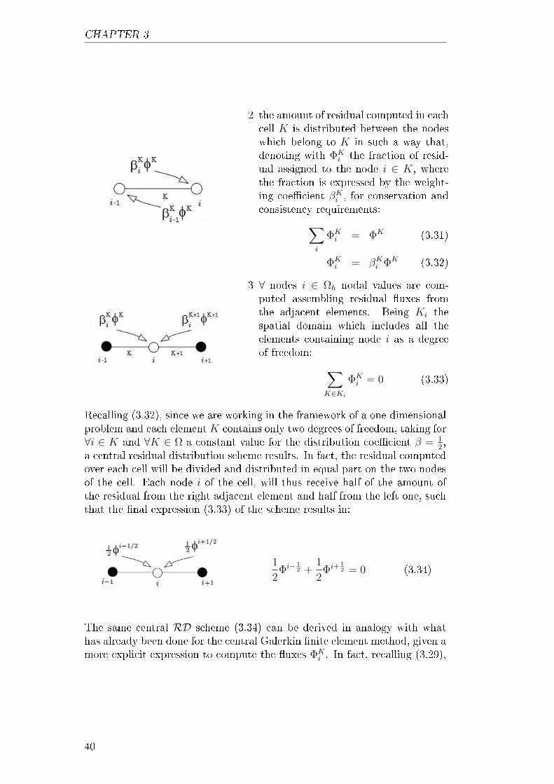
CHAPTER 3

2 the amount of residual computed in eachcell K is distributed between the nodeswhich belong to K in such a way that,denoting with ΦK

i the fraction of resid-ual assigned to the node i ∈ K, wherethe fraction is expressed by the weight-ing coecient βKi , for conservation andconsistency requirements:∑

i

ΦKi = ΦK (3.31)

ΦKi = βKi ΦK (3.32)

3 ∀ nodes i ∈ Ωh nodal values are com-puted assembling residual uxes fromthe adjacent elements. Being Ki thespatial domain which includes all theelements containing node i as a degreeof freedom: ∑

K∈Ki

ΦKi = 0 (3.33)

Recalling (3.32), since we are working in the framework of a one-dimensionalproblem and each element K contains only two degrees of freedom, taking for∀i ∈ K and ∀K ∈ Ω a constant value for the distribution coecient β = 1

2,

a central residual distribution scheme results. In fact, the residual computedover each cell will be divided and distributed in equal part on the two nodesof the cell. Each node i of the cell, will thus receive half of the amount ofthe residual from the right adjacent element and half from the left one, suchthat the nal expression (3.33) of the scheme results in:

1

2Φi− 1

2 +1

2Φi+ 1

2 = 0 (3.34)

The same central RD scheme (3.34) can be derived in analogy with whathas already been done for the central Galerkin nite element method, given amore explicit expression to compute the uxes ΦK

i . In fact, recalling (3.29),

40

LINEAR SCALAR ADVECTION EQUATION

using the Galerkin linear basis functions ϕi presented in the previous sectioninstead of the generical constant weighting functions ωi, the expression forthe node i of the grid will be:

∫ i+1

i−1

ϕi (∂tuh + a∂xuh) dx = 0 (3.35)

If now the middle point quadrature rule is used, instead of the Simpson one,to approximate denite integrals of the (3.35), since the new quadrature rulerepresents the exact evaluation of denite integral of linear functions, theresulting expression will be coincident with that of equation (3.23), exceptfor the coecient of the mass matrix. We have:

∆x

4

d(ui−1)

dt+

∆x

2

d(ui)

dt+

∆x

4

d(ui+1)

dt+a

2(ui+1 − ui−1) = 0 (3.36)

Finally, being Φi− 12 the residual computed over the left adjacent cell to node

i, having it the extremes in i and i−1, it can be assigned the following values:

Φi− 12 = ∆x

d(ui−12 )

dt+ a (ui − ui−1) (3.37)

such that (3.36) can be rewritten as:

1

2Φi− 1

2 +1

2Φi+ 1

2 = 0 (3.38)

and the connection with (3.34) is shown.

Truncation Error : A further conrmation of the great accuracy propertyguaranteed by the Galerkin mass matrix comes from the accuracy order fall(from fourth to second) caused by the changing of the matrix coecients,which is due to the dierent quadrature rule used in the integration of (3.35).Using Fourier expansion to express the degrees of freedom i−1 and i+1, asdone for the previous methods, the following expression is obtained:

41

CHAPTER 3

∂tui + a∂xui =− ∆x2

2∂x2

(1

2∂tui +

a

3∂xui

)+

− ∆x4

24∂x4

(1

2∂tui +

a

5∂xui

)+ O(∆x6)

(3.39)

which shows a O(∆x2) truncation error of the scheme, if the exact solutionfor the linear scalar advection problem is assume to be substituted to therst term of the expression.

Dispersion Analysis : The dispersion analysis of the central residual dis-tribution scheme (3.38) requires the same passages used for the Galerkinmethod, since the two schemes are almost the same. Consequently, by ap-plying the same procedure, a very similar expression for parameters ξ and ωcan be found:

ξRD = 0 (3.40)

ωRD = −ak sinµ∆x

µ∆x

2

1 + cosµ∆x

(3.41)

Comparing (3.41) with (3.28), it becomes evident that the main dierencebetween the two expressions consists in the factor which results from the massmatrix formulation. We have already shown how the residual distributionmass matrix worsens the high properties guaranteed by Galerkin ones; thisis true also for the dispersion accuracy (see Figure 3.4).Central residual distribution scheme (3.38) performed worst with respect tothe Galerkin fourth order accuracy method, but shows a better reconstructionof the properties of the model with respect to the other second order nitedierence scheme. The damping parameter ξ is always correctly null.

42

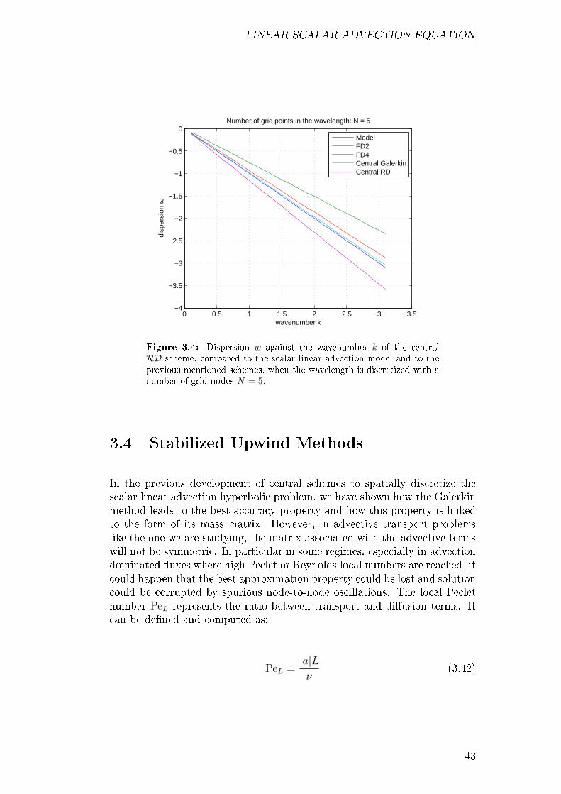
LINEAR SCALAR ADVECTION EQUATION

0 0.5 1 1.5 2 2.5 3 3.5−4

−3.5

−3

−2.5

−2

−1.5

−1

−0.5

0Number of grid points in the wavelength: N = 5

wavenumber k

disp

ersi

on ω

ModelFD2FD4Central GalerkinCentral RD

Figure 3.4: Dispersion w against the wavenumber k of the centralRD scheme, compared to the scalar linear advection model and to theprevious mentioned schemes, when the wavelength is discretized with anumber of grid nodes N = 5.

3.4 Stabilized Upwind Methods

In the previous development of central schemes to spatially discretize thescalar linear advection hyperbolic problem, we have shown how the Galerkinmethod leads to the best accuracy property and how this property is linkedto the form of its mass matrix. However, in advective transport problemslike the one we are studying, the matrix associated with the advective termswill not be symmetric. In particular in some regimes, especially in advectiondominated uxes where high Peclet or Reynolds local numbers are reached, itcould happen that the best approximation property could be lost and solutioncould be corrupted by spurious node-to-node oscillations. The local Pecletnumber PeL represents the ratio between transport and diusion terms. Itcan be dened and computed as:

PeL =|a|Lν

(3.42)

43

CHAPTER 3

where ν represent the diusivity coecient, a is the advection velocity and La local reference length, such as the size of the grid element ∆x. In accordanceto its denition, instabilities in central methods computations originate whenPeL > 1 [12]. Equation (3.1) is a pure advection equation, which means thatPeclet local number will be theoretically innite and the solution computedcould result inaccurate.Unless the time integration is carefully chosen (e.g. an implicit method) theGalerkin method shows spurious modes for time-dependent advection. Thesemodes cannot be eliminated for steady state computations, and are relatedto the uniqueness of the solution of the algebraic system associated to thescheme. In particular, the matrix associated to the bilinear Galerkin formb(u, v) = −

∫Ωauh∂xvhdx results singular; this implies an innite number of

solutions which originate spurious modes.A way to eliminate this kind of instabilities and oscillations in the solution isto make a severe renement of the mesh, such that advection no longer dom-inates on the element level. Of course mesh renement is not always possibleand deeply inuences the computational cost of the solution calculation, forthese reasons an alternative to the Galerkin formulation is needed which doesnot exhibit these spurious oscillations. Additional stabilizing terms can alsobe used to control oscillations in presence of large gradients and local discon-tinuous proles [19], [38]. Upwind dierentiation of the advective term allowsto obtain a solution free from spurious contaminations and instabilities: up-wind dierencing amounts to approximating the advective derivatives withsolution values at the upstream and central nodes of a three points stencil.In dependence of the value of the advection velocity a, equation (3.1) can bediscretized as:

d(ui)

dt+a+

∆x(ui − ui−1) = 0 (3.43)

d(ui)

dt+a−

∆x(ui+1 − ui) = 0 (3.44)

although this approximation of the rst spatial derivative is only rst orderaccurate and, thus, it is necessary to renounce to the second order accuracyof the central nite dierence methods (3.10). This loss of accuracy is man-ifested in over-diuse solutions.Upwinded advective terms can be built by simply adding articial diusionto a central scheme. In fact a combination of a central scheme with an up-wind diusive term gives better results with respect to a central scheme or

44

LINEAR SCALAR ADVECTION EQUATION

an upwind one alone. However upwind stabilisation will be useless or evencan produce worse results in ows where Peclet number is PeL < 1, due tothe fact that central Galerkin is already a stable and more accurate methodfor these uxes.In the nite element framework the diusive upwind term can be computedin several dierent ways. The rst idea is to employ modied weighting func-tions ωi to achieve the upwind eect. In general the element upstream a nodeis weighted more heavily than one downstream. In the one-dimensional case,like the one here treated, articial diusion, when optimally selected, bal-ances the negative diusion inherent in the Galerkin method, thus resulting inthe exact nodal solutions for the model problem. However multidimensionalgeneralisation can be unsuccessful due to crosswind diusion problems. Inthe Streamline Upwind Petrov-Galerkin weighted residual method (SU/PG)the basic idea is to add diusion (or articial viscosity) in the ow direc-tion only. Thus, standard Galerkin weighted functions must be modied byadding a streamline upwind perturbation, which again acts only in the owdirection. The modied weighting functions can then be applied to all theterms of the governing equation, resulting in this way in a consistent weightedresidual formulation [36], [38].In Galerkin formulation weighting functions are considered to be continuousacross inter-elements boundaries. The streamline upwind Petrov-Galerkinmethod requires, instead, discontinuous weighting functions ωi which can beobtained summing to the continuous central functions ϕi the discontinuousstreamline upwind contributions δϕi:

ωi = ϕi + δϕi (3.45)

For what discussed above, the general SU/PG formulation for the one-dimensional linear scalar advection problem results in the following form:

∫Ω

ϕi∂tuhdx+

∫Ω

ϕia∂xuhdx+∑K∈Ω

∫K

δϕi (∂tuh + a∂xuh) dx = 0 (3.46)

being the expression for the streamline upwind weighting operator:

δϕi = a ∂xϕi τ (3.47)

45

CHAPTER 3

τ is a scale parameter which controls the quantity of articial viscosity in-serted into the model and is set such as τ = ∆x/(2|a|). The upwind termadded to the Galerkin scheme in equation (3.46), increases the weight of theleft ux, and diminishes the right one, under the hypothesis of a positiveadvection velocity a > 0, since the gradient ∂xϕi is positive over the leftadjacent cell of node i, and is negative over the right one. Therefore the one-dimensional Galerkin linear weighted functions of Figure 2.1 are modiedobtaining the discontinuous ωi which assumes a shape like the one shown inthe following Figure 3.5.

Figure 3.5: Representation of the upwind linear nite basis functionover the element e.

Introducing the residual ΦK denined as in (3.30), and being CS the cen-tral scheme which has to be stabilized, formulation (3.46) can be rewritten,referred to a generic internal node of the mesh, as:

CS +sign(a)

2Φi− 1

2 − sign(a)

2Φi+ 1

2 = 0 (3.48)

Let now CS be the central Galerkin nite element discretization of the linearscalar advection (3.1), then the scheme resulting can be recast as:

5∆x

12

d(ui−1)

dt+

2∆x

3

d(ui)

dt− ∆x

12

d(ui+1)

dt+ a (ui − ui−1) = 0 (3.49)

In (3.49), as a conrmation of the fact that an upwind weight has beenapplied to the Galerkin central nite element scheme, it could be noted that

46

LINEAR SCALAR ADVECTION EQUATION

the advection ux results approximated with the rst order upwind nitedierence (3.43) and that the coecients of the mass matrix are no moresymmetric in a way such that, since a has been assumed positive, moreweight is given to the upwind node i−1 and less to the downwind one i+1.The form of equation (3.48) suggests to create a SU/PG-type stabilizedscheme using the just developed central residual distribution scheme, insteadof the Galerkin one. In this case, in fact, the method which could be obtained,would be an upwind residual distribution scheme, respecting the formulation:

∑K∈Ω

βKi ΦK = 0 (3.50)

with the distribution coecients over the cell βKi now given by the sum ofthe central weighting functions and the upwind ones in perfect analogy withthe SU/PG just developed:

βKi =1

2+

sign(a)

2(3.51)

In this case, the upwind scheme will simply result:

Φi− 12 =

∆x

2

d(ui−1)

dt+

∆x

2

d(ui)

dt+ a (ui − ui−1) = 0 (3.52)

which even reduces the stencil of only two nodes, although diminishing thehigh order accuracy guaranteed by the SU/PG method, as it will be shownin the following.

Troncation Error : Streamline upwind Petrov-Galerkin method is a con-sistently stabilized method, due to the fact that, in contrast with what seenfor nite dierence upwind method (3.43) and (3.44), the order of the centralGalerkin approximation will not be aected. Truncation error analysis madeon the scheme related to equation (3.49) reveals that a third order accuracyis preserved:

47

CHAPTER 3

∂tui + a∂xui =∆x

2∂x (∂tui + a∂xui) +

− ∆x2

6∂x2 (∂tui + a∂xui) +

+∆x3

12∂x3

(∂tui +

a

2∂xui

)+ O(∆x4)

(3.53)

The analogous upwind method made by central residual distribution schemeshows instead a second order accuracy, which, even being lower with respectto the streamline upwind Petrov-Galerkin one, at least preserves the trunca-tion accuracy of its central scheme.

∂tui + a∂xui =∆x

2∂x (∂tui + a∂xui) +

− ∆x2

2∂x2

(1

2∂tui +

a

3∂xui

)+ O(∆x3)

(3.54)

Dispersion Analysis : Dispersion analysis of the stabilized methods re-sults in more complicated expression for variables ξ and ω of these schemes.Taking into account the SU/PG scheme (3.52), written separating the centralscheme contribution from the stabilizing term in the form:

∆x

6(∂tui−1 + 4∂tui + ∂tui+1) +

a

2(ui+1 − ui−1) +

+∆x

4(∂tui−1 − ∂tui+1)− a

2(ui+1 − 2ui + ui−1) = 0 (3.55)

the generic Fourier mode can now be inserted into (3.55) obtaining the com-plex equation:

2 + cos(µ∆x)

3ν + iak

sinµ∆x

µ∆x

− iν

2sinµ∆x +

ak

µ∆x

(1− cos(µ∆x)) = 0 (3.56)

with ν = ξ + jω and µ∆x = k∆x. Cause to the upwind term, the previousequation results in a coupled system of the two equations for the real and

48

LINEAR SCALAR ADVECTION EQUATION

imaginary part. This lead to an expression for the damping ξ, which is nomore zero as in the central Galerkin scheme, while the expression of ω veryclearly shows the two contributions given by the central and stabilizationterms. In particular we have:

ξSU/PG =

aksin2 µ∆x

2µ∆x

− ak(1− cosµ∆x)2 + cos(µ∆x)

3µ∆x

(2 + cosµ∆x)2

9+

sin2 µ∆x

4

(3.57)

ωSU/PG =

−ak sinµ∆x

µ∆x

+sinµ∆x

2ξSU/PG

2 + cosµ∆x

3

(3.58)

The same analysis, done for the upwind residual distribution scheme (3.52),gives similar results:

ξU/RD =

aksin2 µ∆x

2µ∆x

− ak(1− cosµ∆x)1 + cos(µ∆x)

2µ∆x

(1 + cosµ∆x)2

4+

sin2 µ∆x

4

(3.59)

ωU/RD =

−ak sinµ∆x

µ∆x

+sinµ∆x

2ξU/RD

1 + cosµ∆x

2

(3.60)

Figure 3.6)compares the expression just found with those of the centralschemes above showing that, as for the truncation order accuracy, the stream-line upwind Petrov-Galerkin method slightly worsens the accurate Galerkindispersion description with respect to the exact model, however showing amuch better behaviour than a rst order completely upwind scheme thank toits Galerkin-type mass matrix. The upwind residual distribution scheme, in-stead, surprisingly seems to not modify dispersion and dissipation propertiesof the central scheme, since even the complicated expression (3.58) results,at the end, to be equal to zero from Figure 3.7.

49

CHAPTER 3

0 0.5 1 1.5 2 2.5 3 3.5−4

−3.5

−3

−2.5

−2

−1.5

−1

−0.5

0Number of grid points in the wavelength: N = 5

wavenumber k

disp

ersi

on ω

ModelFD2FD4Central GalerkinCentral RDSU/PGU/RD

Figure 3.6: Dispersion w against the wavenumber k of the stabilizedupwind schemes, compared to the scalar linear advection model andto the previous mentioned schemes, when the wavelength is discretizedwith a number of grid nodes N = 5.

0 0.5 1 1.5 2 2.5 3 3.5−0.25

−0.2

−0.15

−0.1

−0.05

0

0.05Number of grid points in the wavelength: N = 5

wavenumber k [0,π]

dam

ping

ξ

ModelSU/PGU/RD

Figure 3.7: Diusion ξ against the wavenumber k of the stabilizedupwind SU/PG and U/RD schemes, compared to the scalar linear ad-vection model, when the wavelength is discretized with a number of gridnodes N = 5.

50

3.5 Conclusions

In this section, we have spatially discretized the one-dimensional linear scalaradvection equation using dierent numerical methods. We have shown thatGalerkin P1 nite element method results in a central scheme with themajor accuracy order compared to central dierence and residual distribu-tion schemes which use the same approximation of the rst order derivativepresent in the equation. The cost, which has to be paid for this higher accu-racy property consists in the inversion of the mass matrix which, however, canbe done eciently due to the fact that it is constant and, once computed, theinverse matrix can be used all along the calculus. It has been illustrated howGalerkin fourth order accuracy and better dispersion properties are directlylinked to the form of its mass matrix and that a nite dierence scheme canresult by directly lumping its mass matrix, as a central residual distributionscheme can be obtained by directly integrating the weak form using a middlepoint quadrature rule; but these methods are only second order accurate.We have spoken about the raise of instabilities and spurious oscillations inadvection dominated uxes like the ones described by equation (3.1),when they are discretized using centred schemes and, thus, of the ne-cessity of adding upwinding terms of streamline articial diusion deriving,in such a way, a stabilized SU/PG method. In particular the upwind termhas been obtained changing the weighting functions of the variational for-mulation. This fact produces a stabilization term in a residual form whichsuggestes the idea of exchanging the centred scheme previously used in theSU/PG derivation (Galerkin) with the RD one. An upwind residual dis-tribution scheme was, hence, derived in perfect analogy with the streamlineupwind articial diusion theory for advection dominated problems stabil-isation. Both are consistently stabilized methods, since they conserved theaccuracy order of their centred part and are, for this reason, preferable withrespect to complete upwind schemes.Dispersion analysis of all this techniques shows that central Galerkin niteelement methods reaches the best performance in the description of the dis-persive behaviour of the model. This high performance are only weaklyworsened by adding a stabilisation term in the SU/PG scheme, which, how-ever, introduces some non-physical dissipation in the scheme, which resultsin a no more null value of the parameter ξ for this upwind method, while itremains surprisingly zero for the upwind residual distribution scheme.

51

CHAPTER 3

52

Chapter 4

Linear Scalar Advection with

Dispersion Equation

One-dimensional advection-dispersion equation is here considered:

∂tu+ a∂xu− α∂x2tu = 0 (4.1)

we recall that the brief notation ∂x2 is used to indicate the recursive appli-cation of the partial derivative with respect to x for two times, while ∂xtindicates the mixed derivative with respect to space and time.Making the hypothesis of ow velocity a and dispersivity α constant andpositive, the local Peclet number of the ow dened in the same way as in(3.42) still has an innite value, and therefore the necessity of stabilizing thecentral schemes with upwind terms is still present and it is desirable to avoidan excessive renement of the mesh.In the following, the central schemes, already proposed for the scalar advec-tion case, are going to be developed in the same way of the previous chapter,showing the major diculties which arise from the presence, in (4.1), of asecond order spatial derivative term. After this, repeating what already donein section 3.4, diusive upwind terms will be added to the centred schemesin order to give them a major stabilization against spurious oscillations.

Dispersion Analysis : In the scalar linear advection-dispersion equation,replacing the Fourier mode u = ueνt+jkx in (4.1), a very simple expression

53

CHAPTER 4

can be obtained:

(1 + αk2)ν + jak = 0 (4.2)

which shows that for the advection with dispersion case:

ξ = 0 (4.3)

ω = − ak

1 + αk2(4.4)

This means that the damping ξ still remains the same as the simple advectionproblem and only the dispersion parameter ω is aected by the additionalterm α∂x2tu, which thus gives to the model a higher dispersion property.

4.1 Finite Dierence Methods

The development of a nite dierence scheme for spatially discretized equa-tion (4.1) follows directly what has been done for the scalar advection equa-tion. In fact rst spatial derivative of the advective term a∂xu is approxi-mated using the already known formulae (3.7) or (3.9). For the dispersiveterm, instead, a formula for the approximation of the second order spatialderivative is needed. Finite dierence formulae which allow to obtain thesecond and fourth truncation error accuracy order are listed below:

d2f

dx2(xi) =

1

∆x2(fi−1 − 2fi + fi+1) + O(∆x2) (4.5)

d2f

dx2(xi) =

1

12∆x2(−fi−2 + 16fi−1 − 30fi + 16fi+1 − fi+2) + O(∆x4) (4.6)

Using (4.5) and (4.6) to discretize the second order spatial derivative, to-gether with the respective (3.7) and (3.9) to discretize the rst order one,the following second and fourth order schemes can be obtained:

54

LINEAR SCALAR ADVECTION WITH DISPERSION EQUATION

d(ui)

dt+

a

2∆x(ui+1 − ui−1)− α

∆x2

(d(ui−1)

dt− 2

d(ui)

dt+d(ui+1)

dt

)= 0 (4.7)

d(ui)

dt+

a

12∆x(ui−2 − 8ui−1 + 8ui+1 − ui+2) +

− α

12∆x2

(−d(ui−2)

dt+ 16

d(ui−1)

dt− 30

d(ui)

dt+ 16

d(ui+1)

dt+

− d(ui+2)

dt

)= 0

(4.8)

Since the formulae used for the approximation of derivatives are centred,central nite dierence schemes result. They could, thus, perform bad whennear-discontinuous behaviour raises in the ux or when advection dominatedux are analyzed. As anticipated in the previous chapter and observed here,the dispersive terms generates a stiness matrix which has to be inverted inorder to obtain the explicit expression for d(ui)/dt, which allows to computethe solution. The previous advantage of this class of methods, that was dueto the fact that any matrix inversion was needed in order to solve the system,is now lost.

Truncation Error : As for the scalar advection case, a truncation erroranalysis of the schemes (4.7) and (4.8) conrms that the enlargement of thestencil allows to raise up to fourth order. A more accurate numerical solutioncould be computed, but an increase of the computational cost must be paid.

∂tui + a∂xui − α∂xxtui =− ∆x2

6∂x2

(a∂xui −

α

2∂xxtui

)+

− ∆x4

120∂x4

(a∂xui −

α

3∂xxtui

)+ O(∆x6)

(4.9)

∂tui + a∂xui − α∂xxtui = −∆x4

30∂x4 (a∂xui − α∂xxtui) + O(∆x6) (4.10)

Dispersion Analysis : Since schemes (4.7) and (4.8) dier from the anal-ogous of the linear scalar advection equation only because of the dispersiveterm, and due to the fact that this discretized term only results in a term

55

CHAPTER 4

multiplying the complex number ν, since it contains a time derivative, this af-fects only the dispersive property of the schemes, leaving the dissipation oneunchanged with respect to the advection case and thus still null. The expres-sion of ξ and ω of the second and fourth order nite dierence schemes arethus listed below. A comparison between the dispersion of the two schemeswith the exact model one is then shown in Figure 4.1.

ξFD2 = 0 (4.11)

ωFD2 = −ak

sinµ∆x

µ∆x

1 +2αk2

µ2∆x

(1− cosµ∆x)

(4.12)

ξFD4 = 0 (4.13)

ωFD4 = −ak

sinµ∆x

3µ∆x

(4− cosµ∆x)

1 +αk2

6µ2∆x

(15− 16 cosµ∆x + cos 2µ∆x)

(4.14)

0 0.5 1 1.5 2 2.5 3 3.5−0.5

−0.45

−0.4

−0.35

−0.3

−0.25

−0.2

−0.15

−0.1

−0.05Number of grid points in the wavelength: N = 5

wavenumber k

disp

ersi

on ω

ModelFD2FD4

Figure 4.1: Dispersion w against the wavenumber k of the nite dif-ference FD2 and FD4 schemes, compared to the scalar linear advectionwith dispersion model, when the wavelength is discretized with a numberof grid nodes N = 5.

56

LINEAR SCALAR ADVECTION WITH DISPERSION EQUATION

4.2 Galerkin nite element method

All the discussions and considerations made in Section 3.2 about the weightedresidual Galerkin method are still valid for the present advection with disper-sion problem. Thus, Galerkin nite element discretization starts rst fromthe weak formulation of the discretized advection-dispersive equation, whichis:

∫Ω

ψi∂tuhdx−∫

Ω

auh∂xψidx+

∫Ω

α∂xψi∂xtuhdx = BCs (4.15)

In (4.15), BCs stands for boundary evaluated terms which derive from theintegration by part and which can result null if appropriate boundary condi-tions are imposed to the problem.Now, recalling the use of P1 centred basis function ϕj to approximate thesolution in the N + 1 degree of freedom of the domain, since in the Galerkinmethod both weighting functions ψi and basis functions ϕj must be chosenfrom the same functional space, (4.15) becomes:

(∫ X2

X1

ϕiϕjdx

)dujdt−(∫ X2

X1

ϕj∂xϕidx

)auj+

+

(∫ X2

X1

∂xϕi∂xϕjdx

)αdujdt

= 0

(4.16)

In this expression a stiness matrix arises from the dispersion term. Its valueis easy to be computed due to the particular form of the chosen functionsand, as in the case of the mass matrix, the integral over the entire spatialdomain can be split into a sum of integrals over the elements which thenresult in a element-by-element assembly procedure. In practice, using theSimpson quadrature formula to solve denite integrals of (4.16) in the exactway, the following expression centred on node i of the mesh is found:

∆x

6

d(ui−1)

dt+

2∆x

3

d(ui)

dt+

∆x

6

d(ui+1)

dt+a

2(ui+1 − ui−1) +

− α

∆x

(d(ui+1)

dt− 2

d(ui)

dt+d(ui−1)

dt

)= 0

(4.17)

57

CHAPTER 4

Simpson integration results into the central second order nite dierence ap-proximation for both rst and second order spatial derivatives. The Galerkinscheme obtained can thus degenerate to the second nite dierence discretiza-tion method (4.7) when a mass lumping procedure is applied.

Truncation Error : Truncation error analysis of this scheme shows thatthe fourth approximation order of the solution, which characterises the methodin the scalar advection case, is here lost. The second order approximationof the spatial derivative of the dispersive term does not allow the Galerkinmass matrix to recover a higher accuracy order. The expression of truncationerror becomes:

TECG =− ∆x2

6∂x2

(∂tui + a∂xui −

α

2∂x2tui

)+

− ∆x4

12∂x4

(1

6∂tui +

a

10∂xui −

α

30∂x2tui

)+ O(∆x6)

(4.18)

Dispersion Analysis : As far as the dispersion properties of the schemeis concerned, the Fourier analysis of the method returns the values:

ξCG = 0 (4.19)

ωCG = −ak

sinµ∆x

µ∆x

(2 + cosµ∆x)

3+ 2

αk2

µ2∆x

(1− cosµ∆x)

(4.20)

For this method, like for the previous nite dierence scheme and for theexact model, the addition of the dispersive term to the linear scalar advec-tion equation does not introduce any dissipation property which, therefore,remains exactly null. The dispersion character of the scheme produces a littleworse simulation of the diusivity of the model with respect to the previouscase because of the lower accuracy order. However Figure 4.2 shows thatthe schemes perform better, or at least at the same level, of a high accuracyfourth order scheme (FD4) until wavenumbers values of about k ≈ 0.8. For

58

LINEAR SCALAR ADVECTION WITH DISPERSION EQUATION

higher values of k, however, even if the behaviour is such that it reaches thesecond order scheme approssimation, a better performance with respect tothe second order nite dierence scheme (FD2) results.

0 0.5 1 1.5 2 2.5 3 3.5−0.5

−0.45

−0.4

−0.35

−0.3

−0.25

−0.2

−0.15

−0.1

−0.05Number of grid points in the wavelength: N = 5

wavenumber k

disp

ersi

on ω

ModelFD2FD4Central Galerkin

Figure 4.2: Dispersion w against the wavenumber k of the Galerkinnite element scheme, compared to the scalar linear advection with dis-persion model and to the previous mentioned schemes, when the wave-length is discretized with a number of grid nodes N = 5.

4.3 Residual distribution method

The derivation of a central residual distribution method of the kind of equa-tion (3.34) for the scalar linear advection with dispersion equation is morecomplicated with respect to what has been done for the other central schemes,simply operating the discretization of the dispersive term α∂x2tu and addingthis to the original scheme computed for the scalar advection equation case.In the same previous way, what has to be done is to evaluate the residualΦK on each element on the mesh. This residual is now:

ΦK =

∫K

(∂tuh|K + a∂xuh|K − α∂x2tuh|K

)dx (4.21)

59

CHAPTER 4

and must then be distributed in equal parts between the nodes which belongto the same elements, such that, from the point of view of each node i ofthe mesh, it is possible to sum all the residual uxes which come from theadjacent nodes in order to obtain its nodal value. We have already illustratedthat in the one-dimensional case it means that the residual computed on acell must be split between the two degrees of freedom of the element suchthat the distribution coecients values assume the value βKi = 1

2and the

spatial discretization scheme simply results in:

1

2Φi− 1

2 +1

2Φi+ 1

2 = 0 (4.22)

In order to compute the exact expression of the spatially discretized residualsΦi− 1

2 and Φi+ 12 of equation (4.22), the following formulation of the original

problem has to be taken into account:

∫Ω

ωi (∂tuh + a∂xuh − α∂x2tuh) dx = 0 (4.23)

Since the possibility to use integration by parts to transfer one spatial deriva-tive on the weighting functions ωi is not allowed and P1 basis functions areused to approximate the nodal values of the problem variable, a possibilityis to rewrite the strong formulation of the advection-dispersion equation ina lower order form, introducing a new variable w to replace the rst or thesecond spatial derivative of u. In Appendix B it is shown that the choice ofthe type of reconstruction results completely arbitrary, thus both maintain-ing the mixed derivative and decreasing the order of the equation to one doesnot inuence the approximation of the dispersion term which, independentlyon the choice, results in the expression:

− α

4∆x

(d(ui+2)

dt− 2

d(ui)

dt+d(ui−2)

dt

)(4.24)

Anticipating the choice that will be done in the complete Madsen-Sørensencontext, we now decide to set:

w = ∂x2u (4.25)

60

LINEAR SCALAR ADVECTION WITH DISPERSION EQUATION

The auxiliary variable, dened in such a way, increases the numbers of un-knowns of the original equation (4.1). The new denition (4.25) must now bediscretized, integrated and solved together with the scalar linear advection-dispersion equation; the system we are going to deal with, thus, results:

∂tui + a∂xui − α∂twi = 0

wi = ∂x2ui(4.26)

Imaging to compute their residual formulation using a P1 weighting func-tion of the kind of Galerkin nite element scheme, and solving the deniteintegrals on the spatial domain using the middle point quadrature rule, sincea residual distribution scheme is searched, the following spatially discretizedschemes can be found:

∆x

4

d(ui−1)

dt+

∆x

2

d(ui)

dt+

∆x

4

d(ui+1)

dt+a

2(ui+1 − ui−1)

− α∆x

4

(d(wi+1)

dt− 2

d(wi)

dt+d(wi−1)

dt

)= 0

∆x

4wi−1 +

∆x

2wi +

∆x

4wi+1 =

1

∆x(ui+1 − 2ui + ui−1)

(4.27)

The mass lumping technique can be applied on the auxiliary equation ofthe system in order to reduce the computational work added to solve it.Computing directly the value of wi through the second order nite dierenceapproximation (4.5) decreases the accuracy of the reconstruction, howeverthe following analysis shows that the spatial truncation error of the schemeis not signicantly aected by this approximation. The rst equation of thesystem (4.27), instead, can now be directly reorganized and written in thedesired residual distribution form:

1

2Φi− 1

2 +1

2Φi+ 1

2 = 0 (4.28)

Φi− 12 is dened as the central residual ux computed on the one-dimensional

cell, enclosed between nodes i and i−1:

61

CHAPTER 4

Φi− 12 = ∆x

d(ui− 12)

dt+ a (ui − ui−1) + ∆x

d(wi− 12)

dt(4.29)

Truncation Error : Truncation error of the residual distribution schememust be computed rst of all by writing the spatially discretized method inthe following form, using (B.11), which is demonstrated in Appendix A tobe equivalent to nite dierent approximation of the dispersive term madeafter the introduction of the auxiliary variable w:

∆x

4

dui−1

dt+

∆x

2

duidt

+∆x

4

dui+1

dt+a

2(ui+1 − ui−1)+

− α

4∆x

(dui+2

dt− 2

duidt

+dui−2

dt

)= 0

(4.30)

Now, introducing in (4.30) the Taylor expansions shown in (3.8), the followingtruncation error expansion can be found:

TERD =−∆x2∂x2

(1

4∂tui +

a

6∂xui −

α

3∂x2tui

)+

− ∆x4

24∂x4

(1

2∂tui +

a

5∂xui −

32

3α∂x2tui

)+

+ O(∆x6)

(4.31)

which shows that the resulting central scheme is still a second order accuracymethod.

Dispersion Analysis : The study of the dispersive and dissipative prop-erties of the central residual distribution method moves on from the schemewritten in the form (4.30) too. The Fourier analysis, in this case leads to theexpression:

62

LINEAR SCALAR ADVECTION WITH DISPERSION EQUATION

ξRD = 0 (4.32)

ωRD = −ak

sinµ∆x

µ∆x

(1 + cosµ∆x)

2+αk2

µ2∆x

sinµ∆x

(4.33)

0 0.5 1 1.5 2 2.5 3 3.5−0.7

−0.6

−0.5

−0.4

−0.3

−0.2

−0.1

0Number of grid points in the wavelength: N = 5

wavenumber k

disp

ersi

on ω

ModelFD2FD4Central GalerkinCentral Residual Distribution

Figure 4.3: Dispersion w against the wavenumber k of the centralRD scheme, compared to the scalar linear advection with dispersionmodel and to the previous mentioned schemes, when the wavelength isdiscretized with a number of grid nodes N = 5.

Making a comparison with (3.40) and (3.41), it can be seen that, exactlyin the same way of other central spatially discretized schemes, the valueof ξ is not perturbed by the presence of the dispersive term and that themain dierence is the expression now assumed by ω. Figure 4.3 provides acomparison between the dissipative property of the several developed centralschemes and those of the exact model, and it is shown that the central RDscheme performs exactly as a second order scheme.

63

CHAPTER 4

4.4 Stabilized Upwind methods

In this work, a type of streamline upwind Petrov-Galerkin method is used tostabilize the central schemes, since a robust discretization scheme is searched,whose stability could be independent from the time integration scheme used,and spurious oscillations which originate from discontinuous or near - discon-tinuous solutions are wanted to be avoided. The advection-dispersion modelis still a non-dissipative model, so the local Peclet number, which representa ratio between the advection and diusion velocities on the elements spacescale, is going to be innite and the ux will be always advection dominated,thus creating the already explained stability problems in the central spatiallydiscretized schemes.In the previous scalar linear advection case, the stabilization technique wasrealized by means of the residual of the equation. Here the aim is to apply thesame procedure to the advection with dispersion problem, thus, adding anarticial streamline residual based term to the central semi-discrete Galerkinand RD schemes of Sections (4.2) and (4.3).

Recalling the general SU/PG formulation for the one-dimensional linearscalar advection problem (3.48), in the advection with dispersion descreteproblem it becomes:

∫Ω

ϕi∂tuhdx+

∫Ω

ϕia∂xuhdx+

∫Ω

∂xϕiα∂xtuhdx +

+∑K

(∫K

δϕiΦKdx

)= 0

(4.34)

being the streamline upwind weighting operator dened as δϕi = a∂xϕiτ ,with the scale parameter set to τ = ∆x/(2|a|), and being ΦK the residualof the advection-dispersion equation computed on the cell K and dened by(4.21).The dispersion term α∂x2tuh can be computed by means of its weak formula-tion in the central Galerkin part of the scheme, but needs to be managed ina dierent way inside the upwind term, since an integration by part, whichcould transfer at least one derivative to the weighting function, is not possi-ble due to the P1-type functions chosen. The problem is analogous to theone we dealt with in the previous section for the development of the centralRD scheme.

64

LINEAR SCALAR ADVECTION WITH DISPERSION EQUATION

A new auxiliary variable was there introduced in order to decrease the orderof the dispersive term. It was dened such that it assumed the reconstructedvalue of the second order spatial derivative of the problem variable computedusing the second order nite dierence formula. Here, we proceed in exactlythe same way, augmenting the number of the variables of the problem which,thus, required to be coupled with another equation in order to be solved. Us-ing the same denition of the auxiliary variable w, the system which results,written in its weak formulation, is:

∫Ω

ϕi∂tuhdx+

∫Ω

ϕia∂xuhdx+

∫Ω

∂xϕiα∂xtuhdx +

+a∆x

2|a|

∫Ω

∂xϕi(∂tuh|K + a∂xuh|K − α∂twh|K

)dx = 0∫

Ω

ϕiwhdx =−∫

Ω

∂xϕi∂xuhdx

(4.35)

Solving the integrals of this system, assuming a positive value of the advectionspeed (a > 0), the following semi-discrete system can be found:

∆x

6

dui−1

dt+

2∆x

3

duidt

+∆x

6

dui+1

dt+a

2(ui+1 − ui−1) +

+α

∆x

(dui+1

dt− 2

duidt

+dui−1

dt

)+

+∆x

4

dui−1

dt− ∆x

4

dui+1

dt− a

2(ui+1 − 2ui + ui−1) +

+∆x

4

dwi+1

dt− ∆x

4

dwi−1

dt= 0

∆x

4wi−1 +

∆x

2wi +

∆x

4wi+1 =

1

∆x(ui+1 − 2ui + ui−1)

(4.36)

which, using the technique of lumping the mass matrix of the second equationof the system to compute the values of wi+1 and wi−1 and substituting theminto the rst equation, results in the more simple expression:

65

CHAPTER 4

5∆x

12

dui−1

dt+

2∆x

3

duidt− ∆x

12

dui+1

dt+ a (ui − ui−1) +

+α

∆x

(1

4

dui+2

dt− 3

2

dui+1

dt+ 2

duidt− 1

2

dui−1

dt− 1

4

dui−2

dt

)= 0

(4.37)

Using the central residual distribution method derived above to compute thecentred part of the SU/PG scheme instead of Galerkin, an upwind residualdistribution method will results, as it has already been shown for the scalaradvection case. This scheme can be written in the simple form:

∑K∈Ω

βKi ΦK = 0 (4.38)

assuming for the distribution coecient of the scheme the expression:

βKi =1

2+

sign(a)

2(4.39)

which results by adding the upwind weight to the centred one.To compute the exact spatial-discrete expression of this method, the samesteps made in the development of the centred scheme must be accomplished.This implies that the use of the variable w, in order to reconstruct the secondorder derivative of the problem variable u, is still needed. The expression ofthe scheme is found to be:

Φi− 12 =

∆x

2

duidt

+∆x

2

dui−1

dt+ a (ui − ui−1) +

− α∆x

2

(dwidt

+dwi−1

dt

)= 0

(4.40)

Through a mass lumped reconstruction of the value of wi, the previous (4.40)becomes nally:

66

LINEAR SCALAR ADVECTION WITH DISPERSION EQUATION

∆x

2

duidt

+∆x

2

dui−1

dt+ a (ui − ui−1) +

− α

2∆x(dui+1

dt− dui

dt− dui−1

dt+dui−2

dt) = 0

(4.41)

which denote a translation of the stencil of the scheme in the upwind directionwith respect to the central residual distribution case.

Truncation Error : The Truncation error of these streamline upwindschemes, calculated using Taylor approximation of nodal values of the dier-ent degrees of freedom which appear in formulae (4.37) and (4.41), resultsfor the SU/PG scheme in the second order accuracy expression:

∂tui + a∂xui − α∂x2tui =∆x

2∂x (∂tui + a∂xui − α∂x2tui) +

− ∆x2

6∂x2

(∂tui + a∂xui −

α

2∂x2tui

)+ O(∆x3)

(4.42)

For the upwind residual distribution scheme the truncation error is still of thesecond order, since the resulting modify expression of the schemes results:

∂tui + a∂xui − α∂x2tui =∆x

2∂x (∂tui + a∂xui − α∂x2tui) +

− ∆x2

2∂x2

(1

2∂tui +

a

3∂xui −

2α

3∂x2tui

)+ O(∆x3)

(4.43)

The previous (4.42) and (4.43) conrm the fact that this upwind methods,built up on the central schemes by adding a stabilization term to the equation,do not aect their initial accuracy.

Dispersion Analysis : The analysis of the dispersion parameters givesopposite results for the two methods. Figure 4.4 gives a representation of

67

CHAPTER 4

the ωSU/PG and ωU/RD (whose formulae are listet below) together with thetrends of all the other centred schemes presented to discretize the linear scalaradvection-dispersion problem. In particular we have that SU/PG performsmuch better even than the high accurate central FD4 scheme, while theU/RD gives a worse description of the dispersive properties of the modelsalso compared to the second accuracy order central RD scheme. This lastscheme appears, thus, not to be particularly indicated for the solution of theadvection-dispersion problem.The analysis of the dissipation parameter (Figure 4.5) shows instead that anon-physical dissipation has been added to the SU/PG model. Eect whichseems to be totally absent in the upwind residual distribution scheme which,indeed, is able to give stability to its central scheme maintaining an optimaldescription of the dissipation parameter of the physical model.The expressions of the dissipation and dispersive parameters, computed forthe two upwind models developed in this section, are reported below:

ξSU/PG =N ξSU/PG

DξSU/PG

(4.44)

N ξSU/PG = ak

sin2 µ∆x

2µ∆x

(1 + 2

αk2

µ2∆x

(1− cosµ∆x)

)+ (4.45)

− ak

µ∆x

(1− cosµ∆x)

((2 + cosµ∆x)

3+ 2

αk2

µ2∆x

(1− cosµ∆x)

)(4.46)

DξSU/PG =

(2 + cosµ∆x

3+ 2

αk2

µ2∆x

(1− cosµ∆x)

)2

+ (4.47)

+sin2 µ∆x

4

(1 + 2

αk2

µ2∆x

(1− cosµ∆x)

)2

(4.48)

ωSU/PG =

−ak sinµ∆x

µ∆x

+sinµ∆x

2

(1 + 2

αk2

µ2∆x

(1− cosµ∆x)

)ξSU/PG

(2 + cosµ∆x)

3+ 2

αk2

µ2∆x

(1− cosµ∆x)

(4.49)

The same analysis, carried out for the upwind residual distribution scheme(4.41), gives similar results:

68

LINEAR SCALAR ADVECTION WITH DISPERSION EQUATION

ξU/RD =N ξU/RD

DξU/RD

(4.50)

N ξU/RD = ak

sin2 µ∆x

µ∆x

(1

2+αk2

µ2∆x

(1− cosµ∆x)

)+ (4.51)

− ak

µ∆x

(1− cosµ∆x)

((1 + cosµ∆x)

2+αk2

µ2∆x

sin2 µ∆x

)(4.52)

DξU/RD =

(1 + cosµ∆x

2+αk2

µ2∆x

sin2 µ∆x

)2

+ (4.53)

+ sin2 µ∆x

(1

2+αk2

µ2∆x

(1− cosµ∆x)

)2

(4.54)

ωU/RD =

−ak sinµ∆x

µ∆x

+sinµ∆x

2

(1 + 2

αk2

µ2∆x

(1− cosµ∆x)

)ξU/RD

(2 + cosµ∆x)

3+ 2

αk2

µ2∆x

(1− cosµ∆x)

(4.55)

0 0.5 1 1.5 2 2.5 3 3.5−0.7

−0.6

−0.5

−0.4

−0.3

−0.2

−0.1

0Number of grid points in the wavelength: N = 5

wavenumber k

disp

ersi

on ω

ModelFD2FD4Central GalerkinCentral RDSU/PGU/RD

Figure 4.4: Dispersion w against the wavenumber k of the stabilizedupwind SU/PG and U/RD schemes, compared to the scalar linear ad-vection with dispersion model and to the previous mentioned schemes,when the wavelength is discretized with a number of grid nodes N = 5.

69

CHAPTER 4

0 0.5 1 1.5 2 2.5 3 3.5−0.07

−0.06

−0.05

−0.04

−0.03

−0.02

−0.01

0

0.01Number of grid points in the wavelength: N = 5

wavenumber k

diss

ipat

ion

ξ

ModelSU/PGU/RD

Figure 4.5: Diusion ξ against the wavenumber k of the stabilizedupwind SU/PG and U/RD schemes, compared to the scalar linear ad-vection with dispersion model, when the wavelength is discretized witha number of grid nodes N = 5.

4.5 Conclusions

Linear scalar advection with dispersion equation was here discretized in spaceapplying all the schemes previously developed in the simple scalar advecioncase. In this procedure, some complications arised from the second orderspatial derivative of the dispersive term in the development of the centralRD method and of the stabilized schemes. In fact, due to the P1 basisfunction chosen for the approximation of the solution over the grid cells, theintroduction of a new auxiliary variable was needed to reformulate the equa-tion in a lower order form before the integration. In order to accomplish this,the auxiliary variable introduced had to assume the reconstructed value ofthe rst or second spatial derivative of the main variable and transformedthe problem into a system of partial dierential equations augmenting thenumber of the unknowns. It has been demonstrated in Appendix A that thechoice related to the derivative to be reconstructed has no inuence on thenal schemes expressions.All the schemes developed were found to suer from a second order trun-

70

LINEAR SCALAR ADVECTION WITH DISPERSION EQUATION

cation error and had to deal with the inversion of, at least, the stinessmatrix of the semi-discrete system which arises from the dispersion term.This fact increases, in particular, the computational cost of the nite dier-ence schemes which, in the previous case, should not compute any matrixinversion. Hence, in this context the cost of the SU/PG scheme appears tobe not so higher with respect to the nite dierence one, having also theadvantage to be more robust.The analysis of the dispersive parameters, instead, showed a very good agree-ment with the original model for the Galerkin and streamline upwind Petrov-Galerkin schemes. In fact, the former performed as a fourth order accuratescheme in the wavenumbers range till k ≈ 0.8 beyond which this accuracydecreased even though remaining better with respect to the FD2 scheme.The latter is able to attain the best results at all (see Figure 4.4) even re-vealing a non-physical non-null trend of the dissipative parameter ω, which,instead, did not aect the upwind residual distribution scheme. This lastscheme, however, appears to be inadeguate for this kind of problem solutionsince its dispersion error results quite big with respect to those of the otherschemes proposed.

71

72

Chapter 5

Madsen and Sørensen system

discretisation

The extended one-dimensional Boussinesq Madsen and Sørensen model hasalready been presented in Section 1.2, but for convenience it is here rewritten:

∂tη + ∂xq = 0

∂tq −Bh2∂x2tq −1

3h∂xh∂xtq + ∂x(uq) + gH∂xη +

− βgh3∂x3η − 2βgh2∂xh∂x2η = 0

(5.1)

A description of the variables and parameters, which compare in system(5.1), has already been given and a dispersion analysis of this model has alsobeen accomplished. In particular, the dissipation and dispersion parametersof the model appeared to be:

ξMS = 0

ω2MS = k2c2 1 + βµ2

1 +Bµ2

(5.2)

In the following sections we are going to extend the space-discrete schemesdeveloped for the two analysed problems the semi-discretized in space one-dimensional scalar linear advection and the advection with dispersion in

73

CHAPTER 5

order to apply them to the more complex MS one. After the development ofall the dierent methods and the discussion of their properties, the resultingsystem of ordinary dierential equations in time is going to be integrated bymeans of a time integration scheme.

5.1 Finite dierence methods

Finite dierence methods can be easily developed even to discretize the com-plex Madsen-Sørensen system of equations simply by directly replacing thespatial derivatives present in (5.1) with the discrete expressions illustratedin Sections 3.1 and 4.1. However, a third order spatial derivative term isincluded in the MS model. Depending on the accuracy order desired for thediscretization, the second and fourth order accuracy formulae for its approx-imation are:

d3f

dx3(xi) =

1

2∆x3(−fi−2 + 2fi−1 − 2fi+1 + fi+2) + O(∆x2) (5.3)

d3f

dx3(xi) =

1

8∆x3(fi−3 − 8fi−2 + 13fi−1 − 13fi+1 + 8fi+2 − fi+3) +

+ O(∆x4)

(5.4)

These formulae lead to some new centred schemes and this is clear by lookingat the symmetry of the coecients which characterize the expressions (5.3)and (5.4). Their application in the discretization of the term ∂x3η is goingalso to enlarge the stencil of the schemes which result. In particular, applyingthe second order approximations (3.7), (4.5) and (5.3), the following semi-discrete scheme can be found:

74

MADSEN AND SØRENSEN SYSTEM DISCRETISATION

dηidt

+1

2∆x(qi+1 − qi−1) = 0 (5.5)

dqidt− Bh2

i

∆x2

(dqi−1

dt− 2

dqidt

+dqi+1

dt

)+

− hi12∆x2

(hi+1 − hi−1)

(dqi+1

dt− dqi−1

dt

)+

+1

2∆x(ui+1qi+1 − ui−1qi−1) +

gHi

2∆x(ηi+1 − ηi−1) +

− β gh3i

2∆x3(−ηi−2 + 2ηi−1 − 2ηi+1 + ηi+2) +

− β gh2i

∆x3(hi+1 − hi−1) (ηi+1 − 2ηi + ηi−1) = 0

The use of (3.9), (4.6) and (5.4) will, instead, lead to the higher accuratescheme:

dηidt

+1

12∆x(qi−2 − 8qi−1 + 8qi+1 − qi+2) = 0 (5.6)

dqidt− Bh2

i

12∆x2

(−dqi−2

dt+ 16

dqi−1

dt− 30

dqidt

+ 16dqi+1

dt− dqi+2

dt

)+

− hi432∆x2

(hi−2 − 8hi−1 + 8hi+1 − hi+2)(dqi−2

dt− 8

dqi−1

dt+ 8

dqi+1

dt− dqi+2

dt

)+

+1

12∆x(ui−2qi−2 − 8ui−1qi−1 + 8ui+1qi+1 − ui+2qi+2) +

+gHi

12∆x(ηi−2 − 8ηi−1 + 8ηi+1 − ηi+2) +

− β gh3i

8∆x3(ηi−3 − 8ηi−2 + 13ηi−1 − 13ηi+1 + 8ηi+2 − ηi+3) +

− β gh2i

72∆x3(hi−2 − 8hi−1 + 8hi+1 − hi+2)

(−ηi−2 + 16ηi−1 − 30ηi + 16ηi+1 − ηi+2) = 0

Albeit very simple to be derived, this class of schemes is not here applied toany test case since they present diculties in modelling irregular geometries

75

CHAPTER 5

in two space dimensions, due to the fact that representation with structuralgrids reveals a lack of accuracy and local mesh adaptation techniques cannotbe developed for such schemes. Moreover they do not present any computa-tional advantage since, as in the advection-dispersion case, a matrix inversionhas to be computed in any case.In the following paragraphs the properties of these two schemes will be inves-tigated on the simpler linearised Madsen and Sørensen system which diersfrom the complete model for the absence of the nonlinear terms and for theassumption of a constant bathymetry value h = h0 = const. The schemes,which results from the application to the linear problem of the second andfourth order nite dierent approximations of the spatial derivatives, arelisted in Appendix C.

Truncation Error : In order to compute the truncation error analysis ofthe nite dierence schemes (C.3) and (C.4), listed in Appendix C, whichare applied to the linearised Madsen and Sørensen problem (1.20), the stan-dard Taylor series expansions in space (3.12) have to be introduced into theschemes. Rearranging the terms, the following modied expression of the(C.3) system appears:

∂tηi + h0∂xui = −h0∆x2

6∂x3ui −

h0∆x4

120∂x5ui + O(∆x6) (5.7)

∂tui −Bh20∂x2tui + g∂xηi − βgh2

0∂x3ηi =

− ∆x2

6∂x2

(−Bh

20

2∂x2tui + g∂xηi −

7

5βigh

20∂x3ηi

)+

− ∆x4

40∂x4

(−Bh

20

9∂x2tui +

g

3∂xηi − βigh2

0∂x3ηi

)+

+ O(∆x6)

(5.8)

while for the system (C.4), the expression becomes:

∂tηi + h0∂xui =h0∆x4

30∂x5ui + O(∆x6) (5.9)

∂tui −Bh20∂x2tui + g∂xηi − βgh2

0∂x3ηi =

= ∆x4∂x4

(− 2

135Bh2

0∂x2tui +g

30∂xηi −

653

10080βigh

20∂x3ηi

)+

+ O(∆x6)

(5.10)

76

MADSEN AND SØRENSEN SYSTEM DISCRETISATION

The substitution of the solution of the original equations of the system∂tη + h0∂xu = 0 and ∂tu − Bh2

0∂x2tu + g∂xη − βgh20∂x3η = 0 results in the

truncation error expression for both the schemes. Due to the fact that all thespatial derivatives are discretized by means of second order approximationformulae in one case and by fourth order accuracy expressions in the other,not being there any mass matrix which multiplies time derivative terms, weare not surprised to discover that the truncation error of the two methods arecoherently respectively O(∆x2) and O(∆x4). Compared to the scalar linearadvection with dispersion equation, the stencil of both the schemes resultsaugmented because of the exigency to approximate a higher order spatialderivative. From the truncation error analysis it becomes still clear, in thesame way as for the two other simplied cases, that under the payment of thecost of an enlargement of the stencil, this FD schemes could achieve higherorder of accuracy.

Dispersion Analysis : In the Section 1.3.2 the dispersion analysis of thelinearised Madsen and Sørensen system has been investigated and it wasshowed that this extended Boussinesq model gives zero damping and a dis-persion with the expression recalled by (5.2). Taking into account nitedierence spatial discretisation (C.3) and (C.4), the Fourier analysis on thismethods gives the results:

ξFD2 = 0 ξFD4 = 0

ωFD2 =NFD2

DFD2

ωFD4 =NFD4

DFD4

(5.11)

where the expression of the quantities NFD2, DFD2, NFD4 and DFD4 arelisted below:

NFD2 = c2k2 sin2 µ∆x

µ2∆x

+ 2βgh30k

4 sin2 µ∆x

µ4∆x

(1− cosµ∆x)

[5pt]DFD2 = 1 + 2Bh2

0k2

µ2∆x

(1− cosµ∆x)

(5.12)

77

CHAPTER 5

NFD4 =c2k2

36µ∆x

(8 sinµ∆x − sin 2µ∆x)2+

+ βh2

0k2

µ2∆x

(sin 3µ∆x − 8 sin 2µ∆x + 13 sinµ∆x)

DFD4 = 1 +Bh2

0k2

6µ2∆x

(15− 16 cosµ∆x + cos 2µ∆x)

(5.13)

Therefore, expressions contained in (5.11) ensure about the well coherentrepresentation of the non dissipative character of the model by the two nitedierence schemes. The description of the dispersive properties is given inFigure 5.1, where the variation of the quantities ωFD2, ωFD4 and ωMS (theexact model dispersion) is shown as function of the product between thewavenumber k and the constant bathymetry depth h0. The Figure showsclearly that the fourth order accurate scheme gives also the more accuratedispersion description, even if it requires a higher computational cost due toits less compact stencil.

0 0.5 1 1.5 2 2.5 3 3.50

1

2

3

4

5

6

h0k

disp

ersi

on ω

Number of grid points in the wavelength: N = 5

Exact MS model ωMS

ωFD2

ωFD4

Figure 5.1: Dispersion w against the wavenumber k of the nite dif-ference FD2 and FD4 schemes, compared to Airy theory value (1.25),when the wavelength is discretized with a number of grid nodes N = 5.

78

MADSEN AND SØRENSEN SYSTEM DISCRETISATION

5.2 Galerkin nite element method

In the present section, the Galerkin nite element spatial discretization methodis going to be developed in the full extended Boussinesq Madsen and Sørensencontext. We are going to base our discussion on what already presented andexplained for the scalar linear advection and linear advection with disper-sion cases. Thus, recalling rst the one-dimensional MS system in its strongform, given in (5.1), the weak formulation of the problem must be take intoaccount, which states:

∫Ω

ϕi∂tηdx−∫

Ω

q∂xϕidx = 0 (5.14)∫Ω

ϕi∂tqdx+B

∫Ω

∂x(ϕih

2)∂xtqdx+

1

3

∫Ω

∂xh∂x (ϕih) ∂tqdx+

−∫

Ω

uq∂xϕidx− g∫

Ω

η∂x (ϕiH) dx+

+ βg

∫Ω

∂x(ϕih

3)∂x2ηdx+

+ 2βg

∫Ω

∂xh∂x(ϕih

2)∂xηdx = 0

(5.15)

which does not contain any boundary term, which would be originated by theintegration by parts, if, for example, a set of periodic boundary conditionshad been imposed to the spatial domain of the problem. This means thesuppression of one degree of freedom since:

η(X1, t) = η(X2, t) ⇒ ∂xη(X1, t) = ∂xη(X2, t)q(X1, t) = q(X2, t) ⇒ ∂xq(X1, t) = ∂xq(X2, t)

(5.16)

A rst look given to the weak form (5.15) immediately reveals that prob-lems will emerge during the discretization procedure, if the set of linear basisfunctions ϕj, chosen to interpolate the nodal values of the variables func-tions, is taken from the P1 functional space, like it has been done up tonow. In fact, in this case, there would be no way to solve the third orderspatial derivative of the variable η and it would be required to the regular-ity of the basis functions ϕj to be high enough for them to belong to a H 2

Sobolev space over the spatial domain Ω, where v ∈H k(Ω) if v ∈ L2(Ω) and

79

CHAPTER 5

(diν/dxi, i = 1, ..., k) ∈ L2(Ω). Therefore, methods involving H 2 quadraticand H 3 cubic spline functions can be used in this case to solve the problem.The most compact H 2 function is the Hermite cubic [14], where the functionand its rst derivative are continuously interpolated over the mesh. Howeverthe aim here is to design a scheme that can be in the future generalized toa two-dimensional nite element method based on unstructured triangulargrids. Although some work has been done on extending Hermite-type inter-polation onto unstructured grids [22], the additional complexity makes themnot feasible for calculation with large meshes.An alternative to use a higher degree of continuity in the nite element basisfunctions is to rewrite the equation in a lower order form, e.g. by introduc-ing a new variable. The strategy has the same nature to the one that waspresented in Section 4.3 when a way to discretize the dispersion term in aresidual distribution context was searched. The same solution adopted thereis here reproposed, hence, to introduce an auxiliary variable to the problemwhereby to decrease the derivation order of this term and allow the use oflinear P1 weighted and basis functions. Proceeding in this way, the newvariable we are going to introduce could assume, in a free way, the approxi-mated value of the rst or the second spatial derivative of η. In Appendix Bwe have demonstrate that the two dierent choices lead, at the end, exactlyto the same discrete expression of the dispersion term. The same equalitycan be demonstrate also in this case (see Appendix D), under the hypothesisof a constant bathymetry. Otherwise, it can be demonstrated that a smalldierence arises due to the quadrature formula used to solve the denite in-tegrals, but it appears not to change the solution in a sensible way. Following[42], we thus introduce the denition of the auxiliary variable wη as:

wη = ∂xxη (5.17)

This variable extends the number of the unknowns of the system, but thecontinuity restrictions on the test space have been dropped. The situationrequires the addition of a new algebraic equation to the system in orderto nd the solution. Denition (5.4) can be used for this scope, and theincreased system in the weak formulation appears as:

∫Ω

ϕi∂tηdx−∫

Ω

q∂xϕidx = 0 (5.18)

80

MADSEN AND SØRENSEN SYSTEM DISCRETISATION

∫Ω

ϕi∂tqdx +B

∫Ω

∂x(ϕih

2)∂xtqdx+

1

3

∫Ω

∂xh∂x (ϕih) ∂tqdx+

−∫

Ω

uq∂xϕidx− g∫

Ω

η∂x (ϕiH) dx+

+βg

∫Ω

w∂x(ϕih

3)dx+

+ 2βg

∫Ω

∂xh∂x(ϕih

2)∂xηdx = 0

(5.19)

∫Ω

ϕiwdx+

∫Ω

∂xϕi∂xηdx = 0 (5.20)

Now, since the unknowns η(x, t) and u(x, t) are spatially approximated bymeans of the set of P1 basis functions ϕj, we need to use the weak for-mulation to transfer one spatial derivative to the test functions only forterms characterized by a second spatial derivative, like the dispersive ones−Bh2∂x2tq and −2βgh2∂xh∂x2η.The spatial discretized approximation of the unknowns in all the domain isproduced by an interpolation over the set of basis functions as in (3.21):

η(x, t) ≈N+1∑j=1

ψj(x)ηj(t) q(x, t) ≈N+1∑j=1

ψj(x)qj(t) (5.21)

The Galerkin nite element discretization can now be computed by splittingthe integrals over the entire spatial domain into a sum of integrals over thesingle cells and accomplishing a nal assembly procedure, computing thesolution over each element, like in (3.20) using the only two basis functionslocal to it. The same discretization procedure must be applied to equation(5.20) too. This generates an auxiliary algebraic system whose mass matrixis approximated in diagonal form through a lumping technique trying toreduce the extra-work required to solve it, but with the price of decreasingthe accuracy of the approximation. However it is going to be shown, in thefollowing, that this fact does not aect the spatial truncation error of theglobal scheme. The central semi-discrete scheme resulted is shown in itsextended form in Appendix E, but it can be simplied in one of the kind:

Aij yi − fi = 0 (5.22)

81

CHAPTER 5

This is a system of ordinary dierential equations in time, where y(t) con-tains all the system unknowns, matrix A results in a constant coecientmatrix, containing the general Galerkin mass matrix shown for the scalarlinear advection and linear advection with dispersion cases, and f(y, t) is anonlinear function of y. The localised nature of the one-dimensional niteelement spatial approximation proposed will generate a matrix A which isalso banded and which can be solved much more eciently than a full matrix.

Truncation Error : Like in Section 5.1, the truncation error of the schemeis computed on the linearized MS system (1.20). Assuming a smooth classicalsolution which allows to use Taylor series expansions in space for nodal valuesof the variables in the several points of the stencil, and then dierentiatingequation (5.17) and using it to replace the wη,i terms in equation (C.4), weobtain the following modied form of the scheme:

∂tηi + h0∂xui =− ∆x2

6∂x2 (∂tui + h0∂xui) +

− ∆x4

24∂x4

(1

3∂tui +

h0

5∂xui

)+ O(∆x6)

(5.23)

∂tui −Bh20∂x2tui + g∂xηi − βgh2

0∂x3ηi =

− ∆x2

2∂x2

(1

3∂tui −

Bh20

6∂x2tui +

1

3g∂xηi − βgh2

0∂x3ηi

)+

− ∆x4

8∂x4

(1

9∂tui −

Bh20

45∂x2tui +

g

15∂xηi −

1

5βgh2

0∂x3ηi

)+

+ O(∆x6)

(5.24)

Equation (5.23) and (5.24) results very close to the previous (5.7) and (5.8).In fact the only dierence between the central Galerkin nite element andFD2 discretization stands in the presence of the mass matrix and, as alreadyunderlined in the previous sections, the two schemes results the same if a masslumping technique is applied to the rst one. Equations (5.23) and (5.24)show a truncation error which is in the order of O(∆x4) regarding the rstequation of the system, while in the order of O(∆x2) for the former one,thus, conrming the statement that the Galerkin mass matrix increases theaccuracy of a second order nite dierence scheme.

82

MADSEN AND SØRENSEN SYSTEM DISCRETISATION

Dispersion Analysis : We consider now the estimation of the Fourierproperties of the semi-discrete system (C.4). The objective is to recall a cor-respondence between the dumping and the phase speeds obtained by directlyreplacing a Fourier mode into the dierential equation with those obtainedby analyzing the modied equation of the scheme. Considering a Fouriermode of the generic variable u(x, t) = u0e

νt+jkx, we can write:

ui+m = eνtejkm∆x = eνtejmµ∆x (5.25)

where it is setted: µ∆x = k∆x. The time derivative can be written as:

∂tui+m = νeνt+jmµ∆x = νuejmµ∆x (5.26)

which allows us to obtain:

(e−jµ∆x

6+

2

3+ejµ∆x

6

)νη +

h0

2∆x

(ejµ∆x − e−jµ∆x

)u = 0 (5.27)(

e−jµ∆x

6+

2

3+ejµ∆x

6

)νu− Bh2

0

∆x2

(ejµ∆x − 2 + e−jµ∆x

)νu +

+g

2∆x

(ejµ∆x − e−jµ∆x

)η +

− βgh20

2∆x3

(ej2µ∆x − 2ejµ∆x + 2e−iµ∆x − e−i2µ∆x

)η = 0

(5.28)

This system can be written in matrix form introducing the vector of thevariables [η, u]. After this, recalling the denition ν = ξ + jω, the analyticaldetermination of the roots corresponding to this eigenvalue problem, aftermany and long manipulations, leads to this nal expression of the dampingξ and phase ω which appear to be:

ξCG = 0 (5.29)

83

CHAPTER 5

ωCG = c2k2 sin2(µ∆x)

µ2

1 + 2βµ2 1− cos(µ∆x)

µ2∆x

2 + cos(µ∆x)

3

(2 + cos(µ∆x)

3+ 2Bµ2

1− cos(µ∆x)

µ2∆x

)(5.30)

The null value of the damping variable ξ means that the spatial discretizedmodel is non-dissipative, in perfect analogy with the Madsen-Sørensen sys-tem's Fourier properties studied in the Section 1.3. The comparison betweenthe ωCG function of the numerical scheme, just obtained, with the one of theoriginal model, presented in Figure 5.2, shows a good agreement betweenthe dispersion characteristic of the two systems. The trend of ωCG appearsto give a description of the dispersive properties which is almost the sameof a fourth order accuracy scheme, being, in contrast, much better than theFD2 schemes despite the two methods adopt the same approximation of thespatial derivatives.

0 0.5 1 1.5 2 2.5 3 3.50

1

2

3

4

5

6

h0k

dis

pers

ion ω

Number of grid points in the wavelength: N = 5

Exact MS model ωMS

ωFD2

ωFD4

ωCG

Figure 5.2: Dispersion w against the wavenumber k of the Galerkinnite element scheme, compared to Airy theory value and to the previousmentioned schemes, when the wavelength is discretized with a numberof grid nodes N = 5.

84

MADSEN AND SØRENSEN SYSTEM DISCRETISATION

5.3 Residual Distribution

Recalling what already said about the residual discretization technique inthe previous chapters, this method is based on the evaluation of the residualover each cell K of the grid. The residual values are then partitioned betweenthe nodes which belong to the same cell, in a way which is dependent on thedistribution coecients βKi and such that, for consistency:

∑K∈Ki

ΦKi =

∑K∈Ki

βKi ΦK = 0 (5.31)

Since in this section a centred residual scheme is searched, then the distri-bution coecients assume a value βKi = 1/2, because two is the number ofthe degrees of freedom which belong to the cell K, in order to attribute toeach of them the same fraction of the entire value of the residual computed.It is very clear that in a one-dimensional problem, excluding the edges ofthe space domain, each degree of freedom of the mesh i belongs to the twocells adjacent to it and, thus, receives a residual ux from each of them. Thesemi-discrete form of the scheme, written for the node i is, hence, always thesame:

1

2Φi− 1

2 +1

2Φi+ 1

2 = 0 (5.32)

The aspect of the rst equation, which composes the MS system, is verysimilar to the scalar advection equation discretised in Chapter 3. There areno diculties in computing the weighted residual uxes which upgrade thesolution in each node i. The residual ux computed over the cell K takesthe form:

ΦKη =

∫K

(∂tηh + ∂xqh) dx (5.33)

Taking into account the element having nodes i and i−1 as extremes, theintegration with the middle point rule, following the procedure illustrated inSection 3.3 leads to the semi-discrete residual ux expression:

85

CHAPTER 5

Φi− 1

2η = ∆x

dηi− 12

dt+ (qi − qi−1) (5.34)

Diculties arise in the treatment of the second equation belonging to the MSsystem, due to the dispersive and high space derivatives terms here present.In order to give a discrete expression to the residuals ΦK

q , the same proceduredeveloped in Section 4.3 must be taken into account to deal with these terms.In particular, in Section 4.3 we have already dealt with dispersive terms ofthe kind α∂x2tu. The Madsen and Sørensen system of PDEs (5.1) containsan analogous term :Bh2∂x2tq, which, therefore, can be discretized using thesame technique previously illustrated. Thus, an auxiliary variable wq needsto be introduced to decrease the order of derivation of this term. Followingthe steps already presented in Section 4.3, we dene wq = ∂x2q and rewritethe dispersive term in a lower order form as: Bh2∂twq, which can be nowintegrated using P1 basis and weighted functions, without passing throughthe weak formulation.The same technique can be applied in order to decrease the order of spatialderivative which characterize the terms: βgh3∂x3η and 2βgh2∂xh∂x2η, whichin the actual form cannot be solved without the use of the weak formula-tion or a set of basis interpolation functions with more restrictive continuityproperties. In the previous section, the reconstruction of the second spacederivative of the variable η has already been introduced, but it was appliedon the only third space derivative term, since the weak form was used tointegrate the other one. In the residual context, instead, the same recon-struction is going to be compute and applied to solve both these terms.In conclusion we have to double the number of unknowns, dening two auxil-iary variables wη and wq for the reconstruction of the second space derivativesof the two original variables η and q:

wη = ∂xxη (5.35)

wq = ∂xxq (5.36)

The residual related to the q-equation, computed on the cell K of the grid,becomes:

86

MADSEN AND SØRENSEN SYSTEM DISCRETISATION

ΦKq =

∫K

(∂tqh − Bh2∂twq,h −

1

3h∂xh∂xtqh+

+ ∂x(uq)h + gH∂xηh − βgh3∂xwη,h+

− 2βgh2wη,h∂xh)dx

(5.37)

The integration of this expression is now possible in the P1 interpolationfunction space and, accomplishing it using the middle point quadrature rule,leads to the semi-discrete form:

Φi− 1

2q = ∆x

dqi− 12

dt−∆xBh2

i− 12

dwi− 12

dt+

− 1

3∆xhi− 1

2(hi − hi−1)

(dqidt− dqi−1

dt

)+

+((uq)i − (uq)i−1

)+ gHi− 1

2(ηi − ηi−1) +

− βgh3i− 1

2(wη,i − wη,i−1) +

− 2βgh2i− 1

2(hi − hi−1)wη,i− 1

2

(5.38)

The two denitions (5.35) and (5.36) are integrated over the domain usingthe middle point rule too. A more explicit approximation is then introduced,such that the matrices multiplying wη,j and wq,j, namely the mass matrices inthe nite element terminology, are approximated in diagonal form or lumped.In this way, like in Section 5.2, the FD2 reconstruction of the second spacederivatives of the quantities η and q results:

wη,i =1

∆x2(ηi+1 − 2ηi + ηi−1) (5.39)

wq,i =1

∆x2(qi+1 − 2qi + qi−1) (5.40)

Finally, using the expressions of the ux residuals (5.34) and (5.38) togetherwith the reconstruction of the high order space derivatives (5.39) and (5.40),the ultimate form of the central residual distribution scheme, referred to an

87

CHAPTER 5

internal i node of the grid, for the one-dimensional Madsen and Sørensensystem of equations can be written. It stands:

1

2Φi− 1

2η +

1

2Φi+ 1

2η = 0

1

2Φi− 1

2q +

1

2Φi+ 1

2q = 0

wη,i =1

∆x2(ηi+1 − 2ηi + ηi−1)

wq,i =1

∆x2(qi+1 − 2qi + qi−1)

(5.41)

Truncation Error : The scheme (5.41), when applied to the linearised

problem (C.1), requires the residual uxes1

2ΦKη and

1

2ΦKu to be computed

using expressions in (C.6). Substituting the Taylor expansions in space intothe resulting system for the generic internal node, and rearranging the terms:

∂tηi + h0∂xui =− ∆x2

2∂x2

(1

2∂tui +

h0

3∂xui

)+

− ∆x4

24∂x4

(1

2∂tui +

h0

5∂xui

)+

+ O(∆x6)

(5.42)

∂tui − Bh20∂x2tui + g∂xηi − βgh2

0∂x3ηi =

−∆x2∂x2

(1

4∂tui −

1

3

Bh20

2∂x2tui +

1

6g∂xηi −

1

4βgh2

0∂x3ηi

)+

− ∆x4

4∂x4

(1

3∂tui −

8

45Bh2

0∂x2tui +g

30∂xηi −

1

10βgh2

0∂x3ηi

)+

+ O(∆x6)

(5.43)

(5.42) and (5.43) state that the truncation error of the scheme is O(∆x2) forboth the equations of the original MS system and its expressions are:

88

MADSEN AND SØRENSEN SYSTEM DISCRETISATION

0 0.5 1 1.5 2 2.5 3 3.50

1

2

3

4

5

6

h0k

disp

ersi

on ω

Number of grid points in the wavelength: N = 5

Exact MS model ωMS

ωFD2

ωFD4

ωCG

ωCRD

Figure 5.3: Dispersion w against the wavenumber k of the central RDscheme, compared to Airy theory value and to the previous mentionedschemes, when the wavelength is discretized with a number of grid nodesN = 5.

TEηRD =

∆x2

2∂x2

(1

2∂tui +

h0

3∂xui

)+ O(∆x4)

(5.44)

TEqRD =∆x2∂x2

(1

4∂tui −

1

3

Bh20

2∂x2tui +

1

6g∂xηi −

1

4βgh2

0∂x3ηi

)+

+ O(∆x4)

(5.45)

Dispersion Analysis : Using the denition of µ and µ∆x given in theprevious sections, the analysis of the dispersion and dissipation of the schemeleads to the following results:

ξRD = 0 (5.46)

89

CHAPTER 5

ωRD = c2k2 sin2(µ∆x)

µ2

1 + 2βµ2 1− cos(µ∆x)

µ2∆x

1 + cos(µ∆x)

2

(1 + cos(µ∆x)

2+Bµ2

2

1− cos(2µ∆x)

µ2∆x

)(5.47)

Due to the centred characteristic of the scheme and to the non-dissipativecharacter of the equations under analysis, the dissipation parameter ξRD iscorrectly null, while the trend of the dispersion ωRD is shown in Figure 5.3.The trend, compared to the other centred schemes here presented, shows aworse representation of the dispersion properties of the model with respectto the higher accurate Galerkin and FD4 schemes, being however better incomparison to the FD2 scheme, which has the same truncation error orderof accuracy.

5.4 Stabilized Upwind methods

In the previous chapter, some stabilized upwind methods have been presentedfor the advection with dispersion problem. The system of extended Boussi-nesq equations we are dealing with now presents very similar characteristicto the equation studied there. Therefore, the exigency of stabilizing the cen-tred schemes just developed in particular ow conditions, in order to createsemi-discrete schemes which are robust independently from the method usedfor the time integration, is still present. Hence, streamline upwind diu-sion technique is applied with the same observations made for the previousadvection-dispersion case, thus, using the residual of the equation in orderto inuence the stability of a given central scheme.Due to the fact that the upwind stabilized term is computed taking intoaccount the verse of propagation of the information, in equation (4.34) theadvection velocity a was taken into account and included in the upwindweighting functions denition (3.47). Here, we have to deal with a systemof PDEs, which, from the theory, may be characterised by two dierent di-rections of propagation of the information. Due to the intrinsic hyperbolicnature of the problem, we will use the Jacobian matrix of the shallow watersystem in order to predict these behaviour of the solution and compute theupwind term.Being R(η, q) = [Rη(η, q) Rq(η, q)]

T the residual of the MS system in thesense of the denition (2.2), and being Rη(η, q) and Rq(η, q) the vectors ofthe residuals of the two equations of the system, the spatially discrete scheme

90

MADSEN AND SØRENSEN SYSTEM DISCRETISATION

that we are going to developed can be written in the general form:

∫Ω

ϕiRdx+∆x

2sign(A)

∫Ω

∂xϕiRdx = 0 (5.48)

being A the Jacobian matrix of the nonlinear shallow water system.The rst integral of equation (5.48) results in the centred Galerkin or residualdistribution schemes just developed in the previous sections, while the second,which represents the real upwind term, is independent on the kind of thecentral scheme used, exactly as in Sections 3.4 and 4.4. In order to beaccomplished, its solution requires, in fact, that the residual R would notcontain any term characterised by a spatial derivative order higher than one.As already explained before, this is due to the particular function spacechosen for the weighting functions ϕi and to the fact that a spatial derivativeis already applied to them. Thus, auxiliary variables have to be dened todecrease the high order derivative terms present in the q-equation of theMS system, similarly to what done in the previous section for the residualdistribution scheme development. The result reached in this way is very nearto what shown in the Section 5.3; the dimension of the system is doubledby means of the introduction of wη and wq for the reconstruction of thesecond order spatial derivative of the original η and q variables and thesame expression of the residual uxes ΦK

η and ΦKq can be found solving the

integrals.In particular, in each system related to the general internal node i of themesh, the upwind term is made by the two contributions given by the leftand right cells adjacent to the node itself, respectively i−1/2 and i+1/2. Inthis context, the 2x2 square matrix A is computed locally on both cells suchthat the resulted scheme, related to the i node, can be written in the form:

CS +sign(Ai− 1

2)

2

[Φi− 1

2η

Φi− 1

2q

]−

sign(Ai+ 12)

2

[Φi+ 1

2η

Φi+ 1

2q

](5.49)

being CS the centred scheme the stabilization is applied to and using (5.34)and (5.38) for the residuals computation. CS represent the MS system spa-tially discretized with a central scheme; thus, referred to a generic internalnode, it becomes a vector including the two semi-discrete equations CSη andCSq of the system, written for the same reference node. If CSη and CSqassume the expressions of the Galerkin nite element discretization (E.1),the streamline upwind Petrov-Galerkin method is obtained. Otherwise, if

91

CHAPTER 5

the central residual distribution approximation (5.41) is there substituted,an upwind residual distribution method is reached.Finally the sign(AK) matrix is computed using a spectral decomposition ofthe local AK , resulting in:

sign(AK) = Rsign(Λ)L

=1

2cK

[1 1

uK − cK uK + cK

]

sign

([uK − cK 0

0 uK + cK

])[uK + cK −1

cK − uK 1

](5.50)

where R and L are respectively the matrices of the right and left eigenvectorsof AK , Λ is a diagonal matrix, which contains the eigenvalues of AK , uK andcK are the values of the local velocity and celerity of the ow.The scheme is applied to the linearised Madsen and Sørensen problem inAppendix C. The resulting form (C.8) will be used in the following para-graphs in order to study the properties of these methods and to comparethem with those of the central schemes illustrated in the previous sections ofthis chapter.

Truncation Error : Substituting the standard Taylor expansions in spaceinto the system (C.8) and rearranging the terms, in the SU/PG case weobtain:

∂tηi + h0∂xui =c∆x

g∂x(∂tui −Bh2

0∂x2tui + g∂xηi − βgh20∂x3ηi

)+

− ∆x2

6∂x2 (∂tui + h0∂xui) +

+c∆x3

2g∂x3

(1

3∂tui −

1

2Bh2

0∂x2tui +1

6g∂xηi −

1

3βgh2

0∂x3ηi

)+

− ∆x4

24∂x4

(1

3∂tui +

h0

5∂xui

)+ O(∆x5)

(5.51)

92

MADSEN AND SØRENSEN SYSTEM DISCRETISATION

∂tui −Bh20∂x2tui + g∂xηi − βgh2

0∂x3ηi =g∆x

c∂x (∂tηi + h0∂xui) +

− ∆x2

2∂x2

(1

3∂tui −

Bh20

6∂x2tui +

1

3g∂xηi − βgh2

0∂x3ηi

)+

+g∆x3

6c∂x

(∂tηi +

h0

2∂xui

)+

− ∆x4

8∂x4

(1

9∂tui −

Bh20

45∂x2tui +

g

15∂xηi −

1

5βgh2

0∂x3ηi

)+

+ O(∆x5)

(5.52)

which means that the expression of the truncation error:

TEηSU/PG =

c∆x3

2g∂x3

(1

3∂tui −

1

2Bh2

0∂x2tui +1

6g∂xηi −

1

3βgh2

0∂x3ηi

)+

− ∆x4

24∂x4

(1

3∂tui +

h0

5∂xui

)+ O(∆x5)

(5.53)

TEuSU/PG =− ∆x2

2∂x2

(1

3∂tui −

Bh20

6∂x2tui +

1

3g∂xηi − βgh2

0∂x3ηi

)+

+g∆x3

6c∂x

(∂tηi +

h0

2∂xui

)+

− ∆x4

8∂x4

(1

9∂tui −

Bh20

45∂x2tui +

g

15∂xηi −

1

5βgh2

0∂x3ηi

)+

+ O(∆x5)

(5.54)

is O(∆x3), relating to the η-equation, and O(∆x2), relating to the q-equationof the MS system. These results conrm that the kind of stabilisation addedto the central Galerkin nite element discretization does not decrease, ordecrease only weakly, its order of accuracy. The results, expecially the onerelated to the η-equation, appear to be in strong analogy with respect towhat obtained in the linear scalar advection case.The same observations arise from the analysis of the U/RD scheme. In thiscase we have:

93

CHAPTER 5

∂tηi + h0∂xui =c∆x

g∂x(∂tui −Bh2

0∂x2tui + g∂xηi − βgh20∂x3ηi

)+

− ∆x2

2∂x2

(1

2∂tui +

h0

3∂xui

)+

+c∆x3

2g∂x3

(1

3∂tui −

1

2Bh2

0∂x2tui +1

6g∂xηi −

1

3βgh2

0∂x3ηi

)+

− ∆x4

24∂x4

(1

2∂tui +

h0

5∂xui

)+ O(∆x6)

(5.55)

∂tui − Bh20∂x2tui + g∂xηi − βgh2

0∂x3ηi =g∆x

c∂x (∂tηi + h0∂xui) +

−∆x2∂x2

(1

4∂tui −

1

3

Bh20

2∂x2tui +

1

6g∂xηi −

1

4βgh2

0∂x3ηi

)+

+g∆x3

6c∂x

(∂tηi +

h0

2∂xui

)+

− ∆x4

4∂x4

(1

3∂tui −

8

45Bh2

0∂x2tui +g

30∂xηi −

1

10βgh2

0∂x3ηi

)+

+ O(∆x6)

(5.56)

which, imaging to substituting the exact solution of the MS system, leadsthe expression of the truncation error:

TEηU/RD =− ∆x2

2∂x2

(1

2∂tui +

h0

3∂xui

)+

+c∆x3

2g∂x3

(1

3∂tui −

1

2Bh2

0∂x2tui +1

6g∂xηi −

1

3βgh2

0∂x3ηi

)+

− ∆x4

24∂x4

(1

2∂tui +

h0

5∂xui

)+ O(∆x5)

(5.57)

94

MADSEN AND SØRENSEN SYSTEM DISCRETISATION

TEqU/RD =−∆x2∂x2

(1

4∂tui −

1

3

Bh20

2∂x2tui +

1

6g∂xηi −

1

4βgh2

0∂x3ηi

)+

+g∆x3

6c∂x

(∂tηi +

h0

2∂xui

)+

− ∆x4

4∂x4

(1

3∂tui −

8

45Bh2

0∂x2tui +g

30∂xηi −

1

10βgh2

0∂x3ηi

)+

+ O(∆x5)

(5.58)

Dispersion Analysis : The analysis of the dispersion properties of boththese upwind schemes leads to the same form of the dispersion and dissipationparameters ξ and ω:

ξ = − Aν2Aν2

(5.59)

ω =

√AsAν2

− ξ2 (5.60)

In the SU/PG scheme, the expressions of the coecients Aν2 , Aν and As arefound to be:

Aν2 =(2 + cosµ∆x)

3

((2 + cosµ∆x)

3+ 2Bµ2 (1− cos (µ∆x))

µ2∆x

)+

+sin2 µ∆x

4

(1 + 2Bµ2 (1− cosµ∆x)

µ2∆x

) (5.61)

Aν = ck(1− cosµ∆x)

µ∆x

((2 + cosµ∆x)

3+ 2Bµ2 (1− cos (µ∆x))

µ2∆x

)+

+ 2βcµ2 (1− cosµ∆x)2

µ3∆x

((2 + cosµ∆x)

3+ 2Bµ2 (1− cos (µ∆x))

µ2∆x

)+

− ck sin2 µ∆x

2µ∆x

(1 + 2Bµ2 (1− cosµ∆x)

µ2∆x

)(1 + 2βµ2 (1− cosµ∆x)

µ2∆x

)+

+ ck(1− cosµ∆x)

2

6µ∆x

(5.62)

95

CHAPTER 5

As = c2k2 (1− cosµ∆x)2

µ2∆x

(1 + 2βµ2 (1− cosµ∆x)

µ∆x2

)+

+ c2k2 sin2 µ∆x

µ2∆x

(1 + 2Bµ2 (1− cosµ∆x)

µ2∆x

) (5.63)

while for the U/RD scheme, these other expressions result:

Aν2 =(1 + cosµ∆x)

2

((1 + cosµ∆x)

2+Bµ2 (1− cos (2µ∆x))

2µ2∆x

)+

+sin2 µ∆x

4

(1 + 2Bµ2 (1− cosµ∆x)

µ2∆x

)

Aν = ck(1− cosµ∆x)

µ∆x

((1 + cosµ∆x)

2+Bµ2 (1− cos (2µ∆x))

2µ2∆x

)+

+ 2βcµ2 (1− cosµ∆x)2

µ3∆x

((1 + cosµ∆x)

2+Bµ2 (1− cos (2µ∆x))

2µ2∆x

)+

− ck sin2 µ∆x

2µ∆x

(1 + 2Bµ2 (1− cosµ∆x)

µ2∆x

)(1 + 2βµ2 (1− cosµ∆x)

µ2∆x

)2

As = c2k2 (1− cosµ∆x)2

µ2∆x

(1 + 2βµ2 (1− cosµ∆x)

µ∆x2

)+

+ c2k2 sin2 µ∆x

µ2∆x

(1 + 2Bµ2 (1− cosµ∆x)

µ2∆x

)

(5.64)

Figure 5.4 and 5.5 shows a comparison between the trend of the previousexpressions of ξ and ω, in dependence of a variation of the wavenumber k.Directly related the two pictures with Fig.4.4 and 4.5 respectively, a stronganalogy can be seen and similar observations can be done.In fact, in the context of the Boussinesq extended equations of Madsen andSørensen as well as in the simple linear scalar advection with dispersion case,the SU/PG scheme is able to give the best approximation of the dispersiveproperties of the model, even with respect to the more accurate FD4. Itsdissipation, however, shows a non-physical trend which reects the articialaddition of dissipation in order to accomplish the stabilisation.On the other hand, the U/RD appears to not change the characteristics ofthe central RD scheme in both the dispersive and dissipation elds.

96

MADSEN AND SØRENSEN SYSTEM DISCRETISATION

0 0.5 1 1.5 2 2.5 3 3.50

1

2

3

4

5

6

h0k

disp

ersi

on ω

Number of grid points in the wavelength: N = 5

Exact modelFD2FD4Central GalerkinCentral RDSU/PGU/RD

Figure 5.4: Dispersion w against the wavenumber k of the stabilizedupwind SU/PG and U/RD schemes, compared to Airy theory value andto the previous mentioned schemes, when the wavelength is discretizedwith a number of grid nodes N = 5.

0 0.5 1 1.5 2 2.5 3 3.5−1.4

−1.2

−1

−0.8

−0.6

−0.4

−0.2

0

0.2

h0k

diss

ipat

ion

ξ

Number of grid points in the wavelength: N = 5

modelSU/PGU/RD

Figure 5.5: Diusion ξ against the wavenumber k of the stabilizedupwind SU/PG and U/RD schemes, compared to Airy theory value andto the previous mentioned schemes, when the wavelength is discretizedwith a number of grid nodes N = 5.

97

CHAPTER 5

5.5 Conclusions

In this chapter the system of extended Boussinesq-type equations of Madsenand Sørensen has been discretized in space applying the schemes already in-troduced in the previous chapters for the simpler linear scalar advection andavection with dispersion cases. The diverse semi-discrete systems of ordinarydierential equations in time, obtained in the various sections of this chap-ter, are thus ready to be integrated in time with an appropriate integrationmethod, such as those that will be described in the next chapter, with theapproximate solution which will be computed at any time by substitutingthe ηj(t) and qj(t) in the (5.21) interpolations over the set of basis functions.In this context, diculties arise from the exigency of approximating high or-der space derivatives of both variables of the problem η and q, which generallyleads to schemes characterised by more extended stencils. The exigency ofdecreasing the order of these terms through the reconstruction of second or-der derivatives, introducing auxiliary variables into the problem, increasesthe dimension of the system doubling the number of variables and equations.However, the approximation of the high order spatial derivative seems to notaect the accuracy of the resulted schemes, exactly as in the scalar linearadvection-dispersion case.The central Galerkin nite element approximation results in a high accuracyfourth order scheme regarding the η-equation, being only second order accu-rate respect to the second equation of the system. Its dispersive properties,however, show a high accordance with respect to the exact dispersion trendof the model, much better than the FD2 which one hand adopts the samereconstruction of the space derivatives, but which on the other hand is notcharacterised by the presence of the Galerkin mass matrix. The stabilizationof the Galerkin scheme, using the residual of the system and the Jacobianmatrix of the shallow water system, in order to compute the direction of prop-agation of the informations, leads to a weakly less accurate scheme, whosedispersion characteristics are, instead, very close to the exact solution oneseven showing an articial trend of the diusive parameter.On the other hand, the central RD scheme derived in Section 5.3 and hisupwind version (Section 5.4) give second order accuracy schemes in both theequations of the system. Their dispersion properties appears to be exactlythe same, which means that the stabilization term does not worsen neitherthe accuracy nor the dispersion of the central scheme. Even the dissipa-tion parameter remains null in this case and does not show any non-physicaltrend.However their properties are worse with respect to Galerkin ones, conrming

98

MADSEN AND SØRENSEN SYSTEM DISCRETISATION

that Galerkin mass matrix gives the better approximation of the solutionand of the dispersive properties of the model with respect to other schemeswhich use the same order of approximation of the spatial derivatives.

99

100

Chapter 6

Time discretization

We are trying to compute an accurate description of the phenomena whichgovern the propagation of gravity waves in the near-shore zone, where thesystem of shallow water equations becomes inaccurate due to the fact that itis not able to describe its dispersion characteristics, which are no more neg-ligible with respect to the nonlinear ones. For this reason, we have chosenthe Madsen-Sørensen system of extended Boussinesq-type equations, havingaccomplished a study of the dispersion properties of this model through acomparison with Airy wave theory.(1.9) is a nonlinear system of partial dierential equations, which, in orderto be solved, requires a space-time discretization. In the previous chapter,several methods were applied to spatially discretised MS system. Each ofthe semi-discrete schemes derived there represents a system of ordinary dif-ferential equations in time which must be now integrated with a proper timeintegration scheme. The general system we have now to deal with, referredto the generic internal node i of the mesh, is one of the kind:

Aij yj − fi = 0 (6.1)

The integration in time of (6.1) leads to a complete discrete model which cannally be implemented and numerically solved. The approximation to thetime derivative y is determined by the time integration method used and tothe order of that method, but has the general form:

yj =yj − zjα∆t

(6.2)

101

CHAPTER 6

where the exact form of zj depends on the time integration algorithm that itis being used and depends on informations inherited from the previous timesteps. In particular z does not depend on the current solution y. Also theconstant α depends on the time integration scheme used, while ∆t representsthe current time step value.Since in general implicit time integration methods are chosen for the betterstability properties which can be reached, the cost of solving a nonlinearproblem with an iterative method must be paid. The equation system issupplied to the time integration algorithm in the form of a residual vector r:

ri = Aij yj − fi (6.3)

The solution is advanced in time by using in (6.3) the approximation (6.2) ofthe time derivative and than by requiring the residual at next time level tobe suciently small. The resulting system of nonlinear equations is solvedusing the classical iterative Newton's method which requires the solution, ateach iteration step, of the linear system:

Jij(y)∆yj = −α∆t ri(y) (6.4)

where ∆y is the solution increment at the current iteration step and Jij(y)is the nonlinear Jacobian matrix of the system given by:

Jij = α∆tdridyi

= α∆tdfidyi− Aij (6.5)

An exact Newton method would require Jij to be recomputed after eachNewton iteration but this would require a matrix factorisation step at eachiteration which would be very expensive in general. This is the most com-putationally part of the time integration process thus convergence propertiesof a scheme are an important eld to be investigated. In order to diminishthe computational eort of the iteration process, it is possible to maintainthe Jacobian constant as long as possible and only to recompute it when theerror given by its approximations exceeds a certain tolerance. In particularthe computation of the Jacobian can be needed in the initial stages when theorder of time integration has not been reached yet and is still growing.Many time-integration methods can be coupled with the description justgiven, but this choice strongly inuences the stability properties of the schemes.

102

TIME DISCRETIZATION

In fact, the semi-discrete methods proposed are weakly stable since the realpart of the amplication coecient (ξ) is null, or weakly negative, for allof them. This means that they must be accurately integrated in time if anuncontrolled divergence of the solution is wanted to be avoid. In particular,an A-stable method maintains the modes of the solution in the negative partof the complex plan, while, on the contrary, this is not guarantee by a notA-stable scheme which can, thus, produce oscillations due to spurious modesif the time step is too coarse. In this work a Crank-Nicolson (CN ) implicitmultistep and A-stable method and a third order Backward DierentiationFormula (BDF3) are implemented. The properties of the resulting numericalschemes are investigated in the following sections.

6.1 Crank-Nicolson time integration method

We present, in this section, the integration of the MS semi-discrete systemsof ordinary dierential equation in time, developed in the previous chapter,using the Crank-Nicolson method. It is an implicit linear one-step methodwhich, for the generic Cauchy problem Au = f(u, t), can compute the valueof the variable at the time n+1 as:

A∆nu =h

2f(u(tn+ 1

2 ), tn+ 12

)(6.6)

where ∆nu = u(tn+1) − u(tn) is the increment and h = ∆t/∆x. Since thefunction f depends on un+1, this is a nonlinear problem, which means thatits solution must be computed as the zero of the function r(w), being:

r(w) = A(w − un)− h

2f(w, tn+1)− h

2f(un, tn) (6.7)

such that r(w) = 0 if w = un+1. Finding the zero of (6.7) means necessaryto use an iterative method as the one described above. Here the classicaliterative Newton's method is applied and written in the form of the system:

wk+1 = wk − J−1r(wk) (6.8)

where J is the Jacobian matrix of the problem and wk is the solution at the

103

CHAPTER 6

iteration step k. The loop starts with w1 = wn and ends setting wkend =un+1, when the convergence conditions are satised, which means whenlog(‖r(wk+1)‖/‖r(w1

)‖ or ‖r(wk+1)‖∞ become less than a xed tolerance

value. Thus the convergence properties of the methods are an importanteld of study and the properties of the numerical schemes here developedwill be investigated in the following sections.Paying the cost of solving a nonlinear problem, better stability propertiescan be reached. Von Neumann stability analysis, in fact shows that Crank-Nicolson scheme has the advantage, with respect to explicit time-integrationschemes, of being neutrally stable, which means that errors remain constantas the computations are carried forward. The method is also A-stable whichmeans that the resulting schemes would be stable and a low CFL number isnot needed for stability but is however required for numerical accuracy.The expression of the matrix A and vector f in (6.3) are strictly dependenton the method chosen to spatially discretize the MS system, between theones derived in Chapter 5. However, in general, matrix A gathers the massmatrix terms together with the ones resulting from the discretization of theoperators Bh2∂x2 and 1

3h∂xh∂x. The vector f , instead, contained all the

other terms discretized in space following the schemes of Chapter 5: ∂x(uq) ,gH∂xη , βgh3∂x3η and 2βgh2∂xh∂x2η.

6.1.1 Truncation Error

The form of the the matrix A and vector f of equation (6.6) depend on thespace discretization scheme adopted. Here, the only study of the truncationerror of these methods are presented. In order to accomplish this, the Taylorexpansion series in time:

un+1 = un+∆t∂tun+

∆t2

2∂t2u

n+∆t3

6∂t3u

n+∆t4

24∂t4u

t+∆t5

120∂t5u

t+ ... (6.9)

has to be taken into account together with the analogous spatial ones in(3.12). The study of the accuracy properties is going to be realized in thelinearised eld of the MS problem, similarly to what has been done in theprevious chapters for all the space-discrete schemes. The space-time discreteschemes, which give a numerical approximation to the linearised MS systemand are here used to accomplish the analysis, can be found in Appendix F.

104

TIME DISCRETIZATION

Galerkin FE scheme with CN time integration : Taking into accountsystem (F.1), introducing the Taylor expansions and rearranging the resultedterms, the following expression can be found:

∂tη + h0∂xu =− ∆t

2∂t (∂tη + h0∂xu)− ∆x2

6∂x2 (∂tη + h0∂xu) +

− ∆t2

2∂t2

(1

3∂tη +

h0

2∂xu

)− ∆t3

12∂t3

(1

2∂tη + h0∂xu

)+

− ∆t∆x2

12∂x2t (∂tη + h0∂xu) +

− ∆x4

24∂4x

(1

3∂tη +

h0

5∂xu

)+ O(∆x5,∆t4)

(6.10)

∂tu−Bh20∂x2tu+ g∂xη − βgh2

0∂x3η =

− ∆t

2∂t(∂tu−Bh2

0∂x2tu+ g∂xη − βgh20∂x3η

)− ∆x2

2∂x2

(1

3∂tu−

1

6Bh2

0∂x2tu+1

3g∂xη −

1

2βgh2

0∂x3η

)+

− ∆t2

2∂t2

(1

3∂tu−

1

3Bh2

0∂x2tu+1

2g∂xη −

1

2βgh2

0∂x3η

)+

+ O(∆x3,∆t3)

(6.11)

Imaging to substitute the exact solution [η, u] of the original system (1.9),the expression of the truncation error of the scheme is obtained:

TEηCG =− ∆t2

2∂2t

(1

3∂tη +

h0

2∂xu

)− ∆x4

24∂4x

(1

3∂tη +

h0

5∂xu

)+

+ O(∆x6,∆t4)

(6.12)

TEuCG =− ∆x2

2∂x2

(1

3∂tu−

1

6Bh2

0∂x2tu+1

3g∂xη −

1

2βgh2

0∂x3η

)− ∆t2

2∂t2

(1

3∂tu−

1

3Bh2

0∂x2tu+1

2g∂xη −

1

2βgh2

0∂x3η

)+

+ O(∆x4,∆t3)

(6.13)

105

CHAPTER 6

(6.12) and (6.13) conrm that Crank-Nicolson time-integration method issecond order accurate in time and also show that the Galerkin accuracy inspace is preserved, since the truncation error is still fourth order for theη-equation and second order for the q-one.

RD scheme with CN time integration : The truncation error of thesemi-discrete residual distribution scheme of Section 5.3 was second orderaccurate in space. The integration with the CN method in time and the studyof the accuracy properties of this fully discrete scheme leads to analogousresults to the ones obtained before for the central Galerkin nite elementmethod. In particular the Taylor expansion of the discrete system, writtenfor the node i of the mesh, leads after some manipulations to the expressions:

∂tη + h0∂xu =− ∆t

2∂t (∂tη + h0∂xu)− ∆x2

2∂x2

(1

2∂tη +

h0

3∂xu

)+

− ∆t2

2∂t2

(1

3∂tη +

h0

2∂xu

)+ O(∆x4,∆t3)

(6.14)

∂tu−Bh20∂x2tu+ g∂xη − βgh2

0∂x3η =

− ∆t

2∂t(∂tu−Bh2

0∂x2tu+ g∂xη − βgh20∂x3η

)−∆x2∂x2

(1

4∂tu−

1

3Bh2

0∂x2tu+1

6g∂xη −

1

4βgh2

0∂x3η

)+

− ∆t2

2∂t2

(1

3∂tu−

1

3Bh2

0∂x2tu+1

2g∂xη −

1

2βgh2

0∂3η

)+

+ O(∆x4,∆t3)

(6.15)

The use of the exact solution of the linearised system in (6.15), gives theexpressions of the truncation errors for the two equations of the MS system:

TEηRD =− ∆x2

2∂x2

(1

2∂tη +

h0

3∂xu

)− ∆t2

2∂t2

(1

3∂tη +

h0

2∂xu

)+

+ O(∆x4,∆t3)

(6.16)

106

TIME DISCRETIZATION

TEuRD =−∆x2∂x2

(1

4∂tu−

1

3Bh2

0∂x2tu+1

6g∂xη −

1

4βgh2

0∂x3η

)− ∆t2

2∂t2

(1

3∂tu−

1

3Bh2

0∂x2tu+1

2g∂xη −

1

2βgh2

0∂x3η

)+

+ O(∆x4,∆t3)

(6.17)

Exactly as in the previous Galerkin case, the spatial approximation accuracyis preserved since the second order of the semi-discrete scheme of Section5.3 is maintained. Moreover, the CN integration method is conrmed to besecond order accurate in time also in this case.

Stabilized upwind schemes with CN time integration : The analysisof the truncation error of the stabilized SU/PG and U/RD schemes leadsto analogous results with respect to the previous two schemes. After theintegration in time, the two methods maintain the general common form(F.3). The details about the expressions which have to be given to thecentral scheme CS or to the residuals ΦK

η and ΦKu , there present, in order to

obtain the two dierent schemes, can be found in Appendix F.Here, recalling the complete expression of the two stabilized upwind schemesfor a generic internal node of the grid, the Taylor expansions in space andtime are computed in the case of the SU/PG scheme rst:

∂tη + h0∂xu = ∆xc

g∂x(∂tu−Bh2

0∂x2tu+ g∂xη − βgh20∂x3η

)+

− ∆t

2∂t (∂tη + h0∂xu)− ∆x2

6∂x2 (∂tη + h0∂xu) +

− ∆t2

2∂t2

(1

3∂tη +

h0

2∂xu

)+

+ O(∆x3,∆t3)

(6.18)

107

CHAPTER 6

∂tu−Bh20∂x2tu+ g∂xη − βgh2

0∂x3η =

+ ∆xg

c∂x (∂tη + h0∂xu) +

− ∆t

2∂t(∂tu−Bh2

0∂x2tu+ g∂xη − βgh20∂x3η

)− ∆x2

2∂x2

(1

3∂tu−

1

6Bh2

0∂x2tu+1

3g∂xη −

1

2βgh2

0∂x3η

)+

− ∆t2

2∂t2

(1

3∂tu−

1

3Bh2

0∂x2tu+1

2g∂xη −

1

2βgh2

0∂x3η

)+

+ O(∆x3,∆t3)

(6.19)

and in the case of the U/RD in the following:

∂tη + h0∂xu = ∆xc

g∂x(∂tu−Bh2

0∂x2tu+ g∂xη − βgh20∂x3η

)+

− ∆t

2∂t (∂tη + h0∂xu)− ∆x2

2∂x2

(1

2∂tη +

h0

3∂xu

)+

− ∆t2

2∂t2

(1

3∂tη +

h0

2∂xu

)+

+ O(∆x3,∆t3)

(6.20)

∂tu−Bh20∂x2tu+ g∂xη − βgh2

0∂x3η =

+ ∆xg

c∂x (∂tη + h0∂xu) +

− ∆t

2∂t(∂tu−Bh2

0∂x2tu+ g∂xη − βgh20∂x3η

)−∆x2∂x2

(1

4∂tu−

1

3Bh2

0∂x2tu+1

6g∂xη −

1

4βgh2

0∂x3η

)+

− ∆t2

2∂t2

(1

3∂tu−

1

3Bh2

0∂x2tu+1

2g∂xη −

1

2βgh2

0∂x3η

)+

+ O(∆x3,∆t3)

(6.21)

The following expression of the truncation errors of the two schemes for thetwo equations of the linearized MS system can now be found. For the SU/PGwe have:

108

TIME DISCRETIZATION

TEηSU/PG =− ∆t2

2∂t2

(1

3∂tη +

h0

2∂xu

)+

+∆x3

2

c

g∂x3

(1

3∂tu−

1

2Bh2

0∂x2tu+1

6g∂xη −

1

3βgh2

0∂x3η

)+

+ O(∆x4,∆t3)

(6.22)

TEuSU/PG =− ∆x2

2∂x2

(1

3∂tu−

1

6Bh2

0∂x2tu+1

3g∂xη −

1

2βgh2

0∂x3η

)+

− ∆t2

2∂t2

(1

3∂tu−

1

3Bh2

0∂x2tu+1

2g∂xη −

1

2βgh2

0∂x3η

)+

+ O(∆x3,∆t3)

(6.23)

In the U/RD case, indeed:

TEηU/RD =− ∆x2

2∂x2

(1

2∂tη +

h0

3∂xu

)− ∆t2

2∂t2

(1

3∂tη +

h0

2∂xu

)+

+ O(∆x3,∆t3)

(6.24)

TEuU/RD =−∆x2∂x2

(1

4∂tu−

1

3Bh2

0∂x2tu+1

6g∂xη −

1

4βgh2

0∂x3η

)+

− ∆t2

2∂t2

(1

3∂tu−

1

3Bh2

0∂x2tu+1

2g∂xη −

1

2βgh2

0∂x3η

)+

+ O(∆x3,∆t3)

(6.25)

which express the preservation of the spatial order of accuracy of the previ-ous semi-discrete schemes developed in Section 5.4 and state one more timethat the Crank-Nicolson integration in time leads to a second order accuratescheme in time. Comparing the expressions of the truncation error formulaejust found with those of the central schemes listed before, we can observethat the upwind term, computed in the general way (5.48) taking into ac-count the residual of the equation, does not aect the expression of any TEu

or TEη, at least at low order terms, which thus remain exactly the same ofthe CS chosen scheme. The only exception to this is given by the TEη

SU/PGwhere the fourth order of accuracy in space is decreased to a third order one,which has, in any case, still a small inuence.

109

CHAPTER 6

6.2 BDF3 time integration method

The backward dierentiation formula (BDF) is a family of implicit meth-ods for the numerical integration of ordinary dierential equations Au(tn) =f(u(tn), tn). They are linear multistep methods, as well as the Crank-Nicolsonmethod, but they approximate the derivative function u of the problem's vari-able at a certain time tn with the values of the variable function itself u(t)at the same time tn and the earlier times. The general form of this class ofschemes can be written as:

p∑j=1

1

jA∆jun+1 = hf(un+1, tn+1) (6.26)

where ∆ denotes the increment operator ∆un=un−un−1; ∆2un=∆un−∆un−1;p represent the number of steps of the scheme and un+1 = u(tn+1).More explicitly, three steps backward dierentiation formula states:

11

6A∆un+1 − 7

6A∆un +

2

6A∆un−1 = hf(un+1, tn+1) (6.27)

The order of this class of methods coincides with their number of steps, whichfor our purposes is three, and the A-stability property characterizes the rsttwo methods of this family. A close inspection of the stability domain for thehigher order BDF methods, included the third order one, shows that someparts very close to the imaginary axis do not produce stable solutions. Theseareas increase their extensions with the order of the scheme and are thus verythin in the case of p = 3. However the implementation of this method tointegrate the schemes proposed, will produce instabilities expecially in thecentred ones, which thus will need low CFL values or high rened meshes inorder to produce stable and accurate results.Applying the BDF3 method (6.27) to the several MS systems of ordinarydierential equation in time, developed in Chapter 5, means that matrix Aand vector f of (6.27) assume a dierent expression in dependence of themethod chosen for the spatial discretization of the original continuum sys-tem (1.9), among the ones derived in this work. However we can say that ingeneral A and f are structured in the same way as was explained for the CNintegration method.In addition, this class of methods are implicit multistep schemes, whichmeans that a Newton iteration process of the kind described before need

110

TIME DISCRETIZATION

to be accomplished on each step in order to compute the solution. Againthis is the most computationally expensive part of the solution process. Avariable wk which change his value at each iteration k has to be introduced.The cycle starts with w1 = un and nishes at wend = un+1 when the samerequirements sets on the residual increment or value are satised. At eachstep we have, thus, to solve for each generic internal node i the problem:

11

6Aij(wj − unj )− 7

6Aij∆u

nj +

2

6Aij∆u

n−1j = hfi(wj) (6.28)

with a proper Newton form of the kind of (6.4), where ri is now:

ri =11

6Aij(wj − unj )− 7

6Aij∆u

nj +

2

6Aij∆u

n−1j − hfi(wj) (6.29)

In particular the BDF3 method is here used to integrate in time the semi-discretized schemes developed in Chapter 5, as an alternative to the previousCrank-Nicolson method, in order to investigate the possibility to obtain ahigher order of the numerical convergence to the exact solution. We haveshown, in fact, in the previous section, that CN is a second order methodin time; using the BDF3, a third order method is searching. A compari-son between the convergence properties of these two integration methods isillustrated in the following, after a brief discussion about numerical imple-mentation of the proposed test.

111

112

Chapter 7

Numerical implementation

In Chapters 5 and 6 respectively the spatial and temporal discretization ofthe Madsen and Sørensen system has been developed in order to obtain afully discrete system which could be implemented and solved in a proper way.In Chapter 5, in particular, we have shown that the solution of the Madsenand Sørensen system using the nite element approach necessary needs therewriting of the system in a low-order form introducing auxiliary variables,resulting in additional equations to be solved. Mass-lumping technique isused on this adding equations in order to reduce the rise in the computa-tional cost of the solution.The extended system so found can be characterized by three PDEs withthree variables (two physical and one auxiliary), as in the case of the Galerkinmethod, or by four PDEs with four (two physical and two auxiliary), as in thecentral RD or in all the stabilized upwind methods proposed. The solutionof the extended system can be accomplished directly including the auxiliaryvariable w into the vector of the variables of the system U = [η q w]T . In sucha way the coupled system can be solved altogether, at each iteration step ofthe Newton iteration process, computing the value ofW k = [ηk qk wk]T andupgrading the value of the solution at the end of the cycle as W end = Un+1.This choice is not the cheapest one.The other possibility, which is here implement, is to separately compute thevalue of the auxiliary variables of the problems, at each iteration step k, us-ing the values of the physical variables computed at the previous step ηk−1,qk−1. The original system of two equations can thus be solved in a coupledway using the just computed value of wk in order to obtain ηk and qk. Theprocedure ends when the convergence requirements are satised, so the valueof the solution can be nally upgraded and the time step incremented.

113

CHAPTER 7

In the following sections we are going to illustrate the environment of the el-ements implemented in order to realize the numerical tests for the validationof the schemes proposed. A method for the computation of the exact formof the soliton wave for the Madsen and Sørensen model, which is going to beused for the test cases, will be shown.Then a brief treatment of the boundaries conditions setted on the test casesproposed in this work will follow, before concluding the chapter with an il-lustration of a method of generating waves internally to the domain, usefulto compute the solutions in tests where the input wave is constant.

7.1 Soliton Wave Generator

A unique standard denition of soliton is dicult to be found in literature,but we refer to it as a self-reinforcing solitary wave that maintains its shapewhile it travels at its constant speed, caused by the cancellation of nonlinearand dispersive eect in the medium where it propagates. Three are the mainproperties of a soliton wave: it has a permanent form, is localized within acertain region (such that it decades or approximates a constant value veryfar in the domain) and can strongly interact with other solitons emergingfrom the collisions unchanged, except for a small phase shift.In the context of the NSWE system, the analytical form of a soliton wave iswell known [29] and described by the formula:

η(ζ) = a sech

(√3a

4h30

(ζ −X0)2

)(7.1)

u(ζ) =

√g

h0

η(ζ) (7.2)

where a is the soliton wave amplitude, h0 the level of the bathymetry, X0 isthe coordinate of the maximum and ζ = x−Ct is a moving coordinate withthe celerity C of the wave.The soliton shape described by (7.1) cannot be applied in the MS context.The study of the propagation of this kind of solution performed using theMadsen and Sørensen model shows a not complete agreement of the obtained

114

NUMERICAL IMPLEMENTATION

wave with the three general features of a soliton wave. In particular a sen-sible amplitude decreasing accompanied by a dispersive wake can be easilyobserved. These eects can be reduced through a mesh renement, but thisstrongly increases the computational coast of the simulations without delet-ing completely the problem.The exact solution of a soliton wave shape for MS system of equations needsto be found in order to achieve better test results. Following what is per-formed in (as in [21], we rst take into account the MS system making thehypothesis of constant bathymetry h0:

∂tη + ∂xq = 0

∂tq −Bh20∂x2tq + ∂x(uq) + g(h0 + η)∂xη − βgh3

0∂x3η = 0(7.3)

h0 is a data of the problem and contributes, together with the will valueof the amplitude a to uniquely dene the shape of the soliton which willresult from this procedure. Assuming that, for a solitary wave solution, it ispossible to write:

η = η(x− Ct) = η(ζ) q = q(x− Ct) = q(ζ) (7.4)

being ζ = x− Ct a moving coordinate with C the celerity of the wave.Using (7.4), the system (7.3) reduces to:

−Cη′ + q′ = 0

−Cq′ + CBh20q′′′ +

(q2

h0 + η

)′+ gh0η

′ +g

2(η2)′ − βgh3

0η′′′ = 0

(7.5)

indicating with the primes the derivatives with respect to the ordinate ζ.(7.5) is now a system of ODEs which can now be integrated.

− Cη + q = 0

− Cq + CBh20q′′ +

q2

h0 + η+ gh0η +

g

2η2 − βgh3

0η′′ = 0

(7.6)

115

CHAPTER 7

Substituting (7.6) into (7.6), a second order ordinary dierential equationfor the ux q can be found. Setting the initial conditions q(0) = qmax andq′(0) = 0, being qmax = C · a through the (7.6), with a the desired waveamplitude, the second order dierential equation is solved numerically inMatlab R© by means of the function ode113. Once obtained the solution q ofthe (7.6), the wave prole η of the soliton is then recollected via (7.6).Since q and η derives from a numerical integration of the ODEs, we do nothave their analytical expressions but only vectors of values which have to beinterpolated over the nodes of the mesh in order to attribute to any degree offreedom of the grid a value of the solution. A particular attention has to bepaid on the tails of the solution returned by the Matlab R© integrator. In orderto avoid a leakage error, it is required to the solution and its derivative to benull and smooth at the tails of the soliton. This kind of error, in fact, aectsnot only the quality of the solution but also the possibility to reconstructthe correct convergence order of the schemes, due to the fact that it cannotbe decreased by using standard techniques, e.g. mesh renement, time stepreduction...

0 2 4 6 8 10 12 14 16 18−1

−0.8

−0.6

−0.4

−0.2

0

0.2

0.4

η

ζ

Figure 7.1: Numerical solution of the integration of the second orderdierential equation of q using the Matlab R© solver ode113.

The solution returned by the Matlab R© solver in general reproduces only onehalf of the soliton shape and is composed by a physical and a non-physical

116

NUMERICAL IMPLEMENTATION

part (see gure 7.1). Necessarily only the rst interesting fraction, where thevalue of the solution is positive, has to be taken into account, cutting therest of the points computed and thus being forced to treat the tail edge inorder to give to the nal shape a continuous trend to zero. In this work, theidea is to reconstruct a dierent shape for the tail by solving the integrationof a new rst order ordinary dierential equation, setting as initial conditionthe value of a point of the tail previously computed. The rst order ODEwe are going to integrate takes origin directly from the second order onespreviously described and has the form [21]:

1

2(q′)2

(−CB +

βgh0

C

)=−

(C2

h0

)q +

(g

2Ch0

)q2+

+

(g

6C2h20

)q3 + C3 ln

(Ch0 + q

Ch0

) (7.7)

0 5 10 15 200

0.02

0.04

0.06

0.08

0.1

0.12

0.14

0.16

0.18

0.2

ζ

η

Initial Soliton ShapeFirst AttemptSecond AttemptThird Attempt

(a)

6.5 7 7.5 8 8.5 9 9.5 10 10.5 11 11.5−1

0

1

2

3

4

5

6

7

8

9

x 10−3

ζ

η

(b)

Figure 7.2: (a): attempts of reconstruction of the tail of the solitonshape by means of the numerical integration of the rst order equation(7.7); (b): close-up of the interest region.

The choice of the point of the tail the integration of (7.7) has to start from isnot trivial. Figure 7.3 shows how it exist an optimum point which producean extension to the tail with good enough continuity properties. Since ananalytical method to nd this point does not exist, a good compromise wasreached after several attempts. In gure 7.2 the nal results of the half ofthe soliton shape, computed with this process, and merging the blue initialsolution with the magenta tail of gure 7.3, is shown.

117

CHAPTER 7

0 2 4 6 8 10 12 14 16 180

0.02

0.04

0.06

0.08

0.1

0.12

0.14

0.16

0.18

0.2

ζ

η

Initial Soliton ShapeFinal Soliton Shape

(a)

6.5 7 7.5 8 8.5 9 9.5 10 10.5 11 11.5−1

0

1

2

3

4

5

6

7

8

9

x 10−3

ζ

η

(b)

Figure 7.3: Optimal solution found for the soliton tail reconstructionand comparison between the nal and the initial conguration (a); close-up of the interest region (b).

To test the goodness of the proposed solution, the propagation of a solitarywave of amplitude a = 0.2 m in still water of constant depth h0 = 1 m hasbeen calculated using the above method to generate the soliton shape andthe MS equations to solve the whole domain. The results of the test (see g-ure 7.4) show a good amplitude and shape conservation without any sensibledispersion eect during the propagation. In gure 7.4(a) the proles, com-puted after constant time steps, are deliberately stacked with the verticalspacing of 0.2 m to show clearly the non-changing amplitude of the prop-agating wave. Figure 7.4(b) shows a comparison between the numericallypredicted and the analytical wave proles plotted against the x axis at thenal time of the simulation t = 69.6 s. The two proles coincide, conrmingthe ability of the numerical model to propagate information at the physicallycorrect speed. Problems which arise during the propagation of the solitonoften involves trailing edge dispersion and consequently reduction in waveheight and celerity. Those phenomena mostly originate from approximationerrors in the governing equations with respect to nonlinearity and disper-sion or a combination of numerical errors from poorly balanced schemes andtruncation of numerical approximation.All the following test cases, performed in the other sections of this work, willbe computed using the soliton shape generator process here developed, whichsimply solves the shape of the soliton wave of amplitude a , xed by the user,able to travel in a stable way over a constant bathymetry conguration h0,data of the test case.

118

NUMERICAL IMPLEMENTATION

0 50 100 150 200 250 300 350

0.2

0ζ

[m]

x [m]

(a)

250 300 350−0.05

0

0.05

0.1

0.15

0.2

0.25

ζ [m

]

x [m]

NumericalExact

(b)

Figure 7.4: (a): evolution of the exact a = 0.2 m solitary wave; (b):comparison between the exact and the numerically computed solitarywave plotted against the spatial domain at the nal time of the simula-tion.

7.2 Boundary conditions

In this work, two kinds of boundary conditions are implemented in order tocompute the test cases proposed: the periodic and the outow boundaries.

Periodic Boundary Conditions : When these kinds of boundary condi-tions are implemented, the informations which arrive to an extreme of the

119

CHAPTER 7

domain are reintroduced on the other side, as if the solution we are lookingat were periodic with a period coincident with the domain of computation,assumed to have non-reecting boundaries.The way to implement this is quite simple because it is enough to set a se-ries of equality conditions on the values of the solution and its derivativesbetween left and right boundaries of the domain.More in detail, imaging to have subdivided the domain into a set of N+1nodes, node 1 and node N+1, which are the extremes of the domain, haveto be considered as the same point, surrounded by the previous node N onthe left and by the following node 2 on the right. In according with thisassumption, the schemes expressions referred to the extreme nodes of thedomain result identically formulated.In addition, depending on the stencil extension of the scheme used, therewill be one or more nodes set near the boundaries such that, if we write theequation of the scheme referred to these nodes themselves, there will be atleast one index in the formula which does not correspond to any real degreeof freedom of the domain. The solution to this problem provided by the im-plementation of the periodic boundary conditions consists of ideally mergingthe two boundaries so that the missing nodes of the formula appear to be onthe other side of the domain.The drawback of this procedure is that the non-zero elements of the matricesof the schemes are no more concentrated along the main diagonals of eachmatrix or of its sub-blocks, but appear to be much sparser.

Outow Boundary Conditions : The aim of an outow boundary is toideally let exit from the domain the informations which trough their propaga-tions arrive to the boundary. In practice they are realized by a non-physicalrestriction of the spatial domain to a suitably smaller one where practicalcomputations can be performed. It is fundamental for these boundaries tominimize non-physical reection of the information back into the computa-tional domain.In this work, a viscous damping layer, termed sponge layer [42], is introducednear the boundary in the form of a viscous term which increases in magni-tude closer to the outow boundary. This viscous term is added to the freesurface equation in the form illustrated below:

120

NUMERICAL IMPLEMENTATION

∂tη + ∂xq = ν∂x2η

∂tq −Bh2∂x2tq −1

3h∂xh∂xtq + ∂x(uq) + gH∂xη +

− βgh3∂x3η − 2βgh2∂xh∂x2η = ν∂x2q

(7.8)

being ν = 0 everywhere but in x ∈ [Xs, X2], being X2 the extreme of thedomain, where it is dened as:

ν = n1e

x−Xs

X2 −Xs

n2

− 1

e1 − 1(7.9)

Here n1 and n2 are constants used to ne tune the amount of viscosity, whichis problem dependent and has to be determined by attempts on each test caseso as to eectively damp the outgoing waves without allowing signicantreections. The width of the sponge layer is another parameter which has tobe varied in order to provide sucient damping for the cases considered.Since the presence of a sponge layer adds a new term to the each of theequations of the MS system. It is important to underline that, althoughformally modifying the expression of the residual, these terms are not takeinto account when the residual of the equation is used in order to computethe stabilization upwind term.

7.3 Internal Wave Generation

For the test cases in which the solution of the interaction between a trainof periodic input waves with a variable bathymetry wants to be compute,the implementation of an oscillating wave-making internal source functionis required in order to produce such train of waves. To obtain the desiredoscillation signal in the wave generating area, following [42], an analogy witha time varying sea bed is drawn, and a new term is added to the η-equationthat simulates the lowest order eects of a time varying depth prole. Thefree surface equation of the MS system, thus, becomes:

∂tη + ∂thI + ∂xq = 0 (7.10)

121

CHAPTER 7

where the form of the sea bed variation hI is taken to be:

hI(x, t) = 2C fI(x) a cos(ωt) (7.11)

where a, C and ω are respectively the amplitude, the celerity and the fre-quency of the required waves and the spatial function fI(x) is given by, stillfollowing [42]:

fI(x) =bI√πe−bI(x−xI)2

(7.12)

These expressions simulate an undulating Gaussian hill centered at the posi-tion x = xI . The width of the generation region results strongly dependenton the value attributed to the parameter bI which, in addition, inuence alsothe amplitude of the oscillation. In particular bI has to be chosen such thatthe function fI(x) is eectively zero at the interfaces between the generationregion and the physical test domain: x = xI ± aI (see the schematic rep-resentation in gure 7.5). Function fI(x) is also normalized, such that itsintegral is one over this region.

Figure 7.5: sketch of the internal wave generation process.

The wave generator just described does not reproduce the correct expectedtrain of periodic waves, but a certain transient is present from the beginningof the oscillation till the generation of a real periodic train of waves. The

122

NUMERICAL IMPLEMENTATION

generator produces both a left and a right travelling wave (as representedin gure 7.5) well reproducing the period and wavelength of the waves evenif an unclear and inexplicated non-correct generation of the amplitudes isregistered. The several parameters which belong to the expressions writtenbefore have thus to be set accurately in a proper way for each test applica-tion.Exactly in the same way as for the sponge layer added term, the term∂thI(x, t) changes the expression of the residual of the continuity equation ofthe system. Even if this term will be treated in the discretization procedureas the similar ∂tη, it will not be taken into account for the stabilization termcomputation.

123

124

Chapter 8

Numerical Tests and Results

In this nal chapter of the work, the properties of the schemes developed andanalysed all along this report are going to be nally tested and veried. Aconvergence study of the methods will be accomplished in order to verify theschemes precision in space-time description for a sequence of rened grids.The ability of these methods to well reproduce nonlinear and dispersion prop-erty of the MS model is going to be tested too, computing the solutions ofthe collision of two solitary waves and of the propagation of a soliton over ashelf in the bathymetry.Finally, at the end of the chapter, the methods of integration proposed arevalidated using the experimental data of a very common test originally pro-posed by [39]: the propagation of a periodic wave over a submerged bar.

8.1 Convergence Analysis

As an indication of the accuracy and eciency of the proposed numerical ap-proaches, we consider the simple propagation of a solitary wave of amplitudea = 0.2 m over an undisturbed depth h = 1 m. The wave is initially centredat x = 50 m and the spatial domain considered is x ∈ [0, 200] m. The soli-ton shape, realized via the procedure described in Section 7.1, is used as theinitial condition and the error e(η) is computed by comparing the resultedsolution after t = 30 s with the same initial shape translated into the spatialdomain of the quantity C · t.The following gure 8.1 shows the form of the error function eη(x), measuredat the nal time of the simulation, when the theoretical solution states that

125

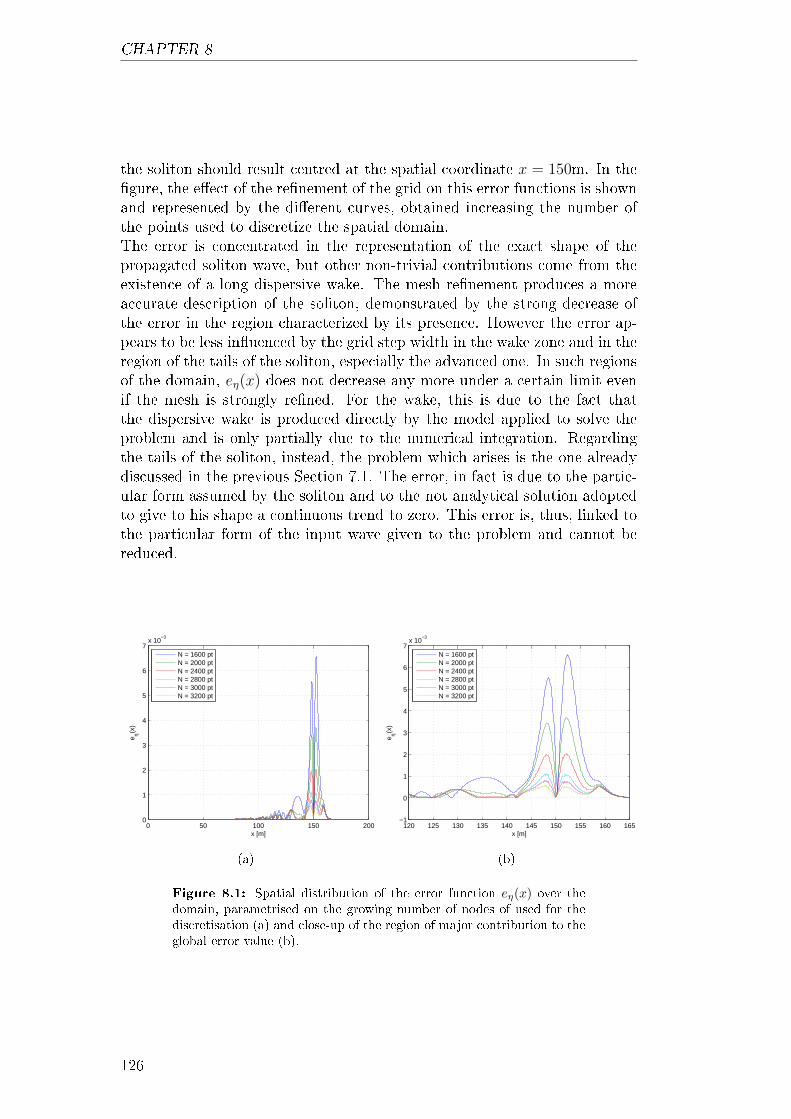
CHAPTER 8

the soliton should result centred at the spatial coordinate x = 150m. In thegure, the eect of the renement of the grid on this error functions is shownand represented by the dierent curves, obtained increasing the number ofthe points used to discretize the spatial domain.The error is concentrated in the representation of the exact shape of thepropagated soliton wave, but other non-trivial contributions come from theexistence of a long dispersive wake. The mesh renement produces a moreaccurate description of the soliton, demonstrated by the strong decrease ofthe error in the region characterized by its presence. However the error ap-pears to be less inuenced by the grid step width in the wake zone and in theregion of the tails of the soliton, especially the advanced one. In such regionsof the domain, eη(x) does not decrease any more under a certain limit evenif the mesh is strongly rened. For the wake, this is due to the fact thatthe dispersive wake is produced directly by the model applied to solve theproblem and is only partially due to the numerical integration. Regardingthe tails of the soliton, instead, the problem which arises is the one alreadydiscussed in the previous Section 7.1. The error, in fact is due to the partic-ular form assumed by the soliton and to the not analytical solution adoptedto give to his shape a continuous trend to zero. This error is, thus, linked tothe particular form of the input wave given to the problem and cannot bereduced.

0 50 100 150 2000

1

2

3

4

5

6

7x 10

−3

x [m]

e η(x)

N = 1600 ptN = 2000 ptN = 2400 ptN = 2800 ptN = 3000 ptN = 3200 pt

(a)

120 125 130 135 140 145 150 155 160 165−1

0

1

2

3

4

5

6

7x 10

−3

x [m]

e η(x)

N = 1600 ptN = 2000 ptN = 2400 ptN = 2800 ptN = 3000 ptN = 3200 pt

(b)

Figure 8.1: Spatial distribution of the error function eη(x) over thedomain, parametrised on the growing number of nodes of used for thediscretisation (a) and close-up of the region of major contribution to theglobal error value (b).

126

NUMERICAL TESTS AND RESULTS

Since a study of the convergence order of the schemes is wanted to be com-puted, it is important to understand this behaviours because, over a certainvalue of the number of the points N used for the discretization, the con-tributes to the global error, which comes from this non-numerical eects,become of the same order of magnitude or even greater with respect to theothers. From the moment in which this happens the order of convergenceof the scheme computed becomes not representative of the real order of thescheme.

In order to perform a convergence study of the schemes proposed and verifythe schemes precision in the space-time description for a sequence of renedgrids, the major requirements is to satisfy a consistency renement property[1]. This property requires the maximum distance across the grid cells to de-crease consistently with an increase of the total number of grid data points.Here, the points of the mesh are equispaced and the mesh renement is ac-complished by increasing the number of degrees of freedom from N = 1600to N = 3200.

In gure 8.2, L2 and L∞ norms of the error and the asymptotic orders ofconvergence are presented for the four central Galerkin, central RD, SU/PGand U/RD schemes integrated in time with the Crank-Nicolson method. Itcan be seen that the schemes do not originate instabilities, conrming thegood property of the A-stable CN method, and the asymptotic order ob-tained for all the schemes is closed to the third and even better.When the BDF3 method is used to integrate in time the same schemes,instead of the CN method, the central Galerkin and residual distributionschemes presents strong oscillations in the solutions for meshes not su-ciently rened and the solution can be computed only with the stabilizedSU/PG and U/RD methods. In particular, this behaviour can be observedin gure 8.3(a) were the trend of convergence of the central Galerkin niteelement scheme is shown. The gure clearly shows the high error levels ob-tained on coarse grids, due to the presence of large numerical oscillations.These instabilities disappear on ned meshes where a fourth order slope isrecovered. It is quite likely that these instabilities are related to the lackof A-stability of the BDF3 method which shows for larger timesteps whenusing the Galerkin scheme in space. In the picture, the trend assumes a veryhigh slope at the beginning before reaching and maintaining a kind of fourthorder convergence slope. This is due to the fact that the renement of themesh planes the numerical oscillations which characterized the solution incoarse grids; thus, the real convergence order of the scheme appears only

127

CHAPTER 8

−3 −2.8 −2.6 −2.4 −2.2 −2 −1.8−10

−9

−8

−7

−6

−5

−4Galerkin FE + CN scheme

log10

(∆ x)

log 10

||e(η

)||

Slope 3L

2L∞

(a)

−3 −2.8 −2.6 −2.4 −2.2 −2 −1.8−10

−9

−8

−7

−6

−5

−4Central RD + CN scheme

log10

(∆ x)

log 10

||e(η

)||

Slope 3L

2L∞

(b)

−3 −2.8 −2.6 −2.4 −2.2 −2 −1.8−10

−9

−8

−7

−6

−5

−4SU/PG + CN scheme

log10

(∆ x)

log 10

||e(η

)||

Slope 3L

2L∞

(c)

−3 −2.8 −2.6 −2.4 −2.2 −2 −1.8−10

−9

−8

−7

−6

−5

−4Upwind RD + CN scheme

log10

(∆ x)

log 10

||e(η

)||

Slope 3L

2L∞

(d)

Figure 8.2: Convergence curves computed for the schemes integratedin time with the Crank-Nicolson method.

after the eects of this instabilities are cancelled. In addition, it was foundimpossible for the centred RD scheme of Section 5.3 to reach convergencewhen BDF3 time integration method is applied; in fact, the graphic of itstrend of convergence is not present between the others of gure 8.3.

The SU/PG, instead, shows a very nice and monotone convergence curveof slope very close to four, while the U/RD scheme yelds a poorer, yetmonotone, grd convergence with averaged slope close to three. In this sense,the SU/PG appears to be the most robust and, hence, the most promisingmethod with respect to the other proposed in this work.

128

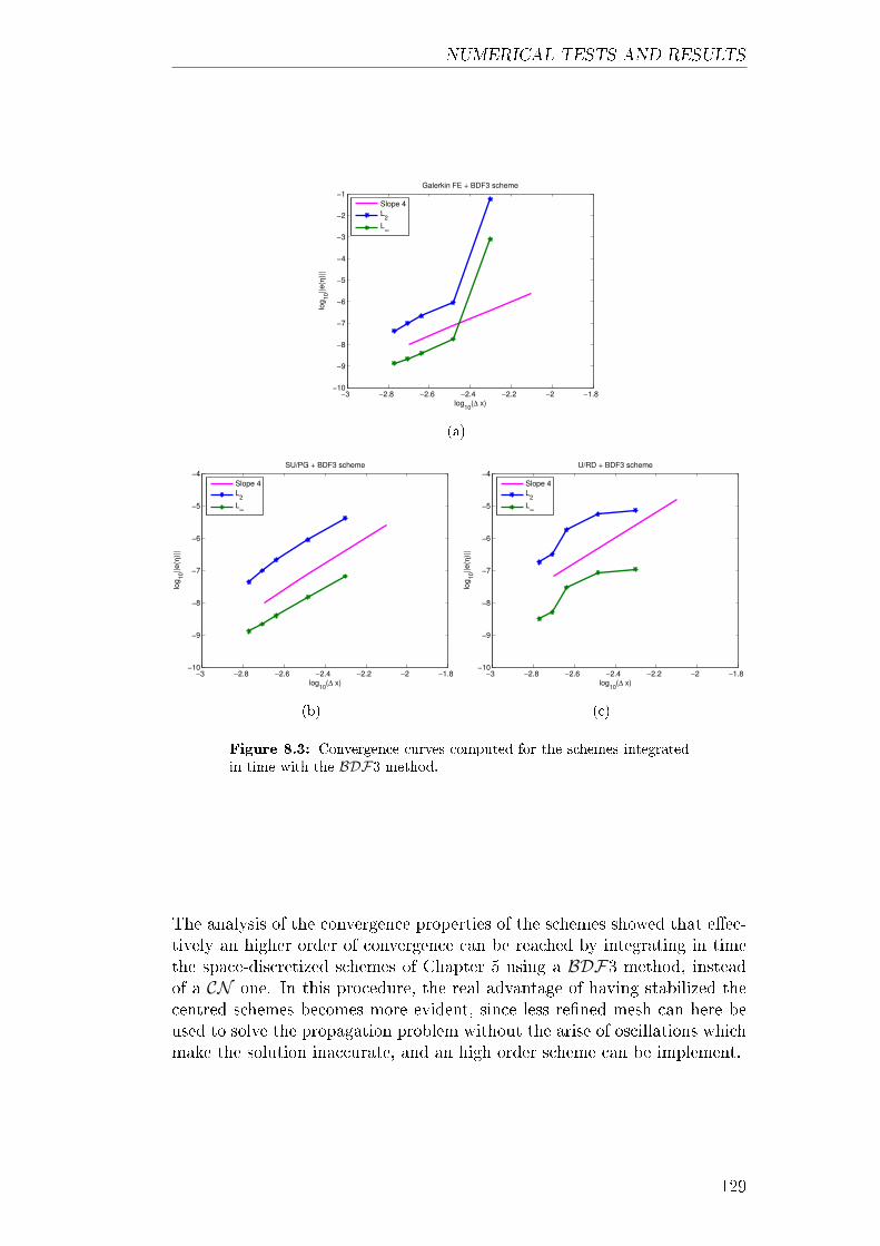
NUMERICAL TESTS AND RESULTS

−3 −2.8 −2.6 −2.4 −2.2 −2 −1.8−10

−9

−8

−7

−6

−5

−4

−3

−2

−1Galerkin FE + BDF3 scheme

log10

(∆ x)

log

10||e

(η)|

|

Slope 4

L2

L∞

(a)

−3 −2.8 −2.6 −2.4 −2.2 −2 −1.8−10

−9

−8

−7

−6

−5

−4SU/PG + BDF3 scheme

log10

(∆ x)

log

10||e

(η)|

|

Slope 4

L2

L∞

(b)

−3 −2.8 −2.6 −2.4 −2.2 −2 −1.8−10

−9

−8

−7

−6

−5

−4U/RD + BDF3 scheme

log10

(∆ x)

log

10||e

(η)|

|

Slope 4

L2

L∞

(c)

Figure 8.3: Convergence curves computed for the schemes integratedin time with the BDF3 method.

The analysis of the convergence properties of the schemes showed that eec-tively an higher order of convergence can be reached by integrating in timethe space-discretized schemes of Chapter 5 using a BDF3 method, insteadof a CN one. In this procedure, the real advantage of having stabilized thecentred schemes becomes more evident, since less rened mesh can here beused to solve the propagation problem without the arise of oscillations whichmake the solution inaccurate, and an high order scheme can be implement.

129

CHAPTER 8

8.2 Head-on Collision of Two Solitary Waves

A common test for the Boussinesq-type and non-hydrostatic models is thesimulation of the interaction of two identical solitary waves propagating inopposite directions. By this numerical test the ability of the scheme to de-scribe the soliton property, already expressed in Section 7.1, to remain un-changed after an interaction with another soliton, wants to be investigate.The collision of the two waves presents additional challenges to the model bya sudden change of the nonlinear and frequency dispersion characteristics.The computation uses a a grid spacing of ∆x = 0.08 m and a time step ofintegration of ∆t = 0.015 s. The domain is assume to be x ∈ [0 200] m withthe initial position of the soliton as represented in gures 8.4(a) and 8.4(b).Both the CN and the BDF3 time integration are implemented for each ofthe four space-discrete schemes proposed.Figure 8.4 represents the simulated surface proles, computed by the inte-gration in time of the SU/PG scheme with both the CN and the BDF3methods, at the beginning of the test, in the instant in which the two wavesexperiment the maximum amplitude of the constructive interference, and atthe end when the two waves have exchange their initial positions. Immedi-ately one can observed that no dierences can be appreciated between theresults given by the two integration methods, which, in addition, show bothan optimal agreement with the theoretical solution at the nal time of thesimulation.Figures 8.5 illustrated, instead, a comparison between the results computedby the several schemes proposed which gives an almost identically descrip-tion of the phenomenon. The nal solution is characterised by the absenceof spurious oscillations and of non-physical dispersion and the nal shape ofthe two waves does not register any relevant variation of their amplitude.Only the residuals schemes shows a weak variation of the phase and overes-timate of the amplitude with respect to the Galerkin and stabilized Galerkinmethods and to the exact analytical solution.

130

NUMERICAL TESTS AND RESULTS

0 50 100 150 200−0.05

0

0.05

0.1

0.15

0.2

Crank − Nicolson

η [m

]

(a)

0 50 100 150 200−0.05

0

0.05

0.1

0.15

0.2

BDF3

η [m

]

(b)

0 50 100 150 200

0

0.1

0.2

0.3

0.4

η [m

]

(c)

0 50 100 150 200

0

0.1

0.2

0.3

0.4

η [m

](d)

0 50 100 150 200−0.05

0

0.05

0.1

0.15

0.2

η [m

]

x [m]

Numerical solutionTheoretical solution

(e)

0 50 100 150 200−0.05

0

0.05

0.1

0.15

0.2

η [m

]

x [m]

Numerical solutionTheoretical solution

(f)

Figure 8.4: Free surface proles of solitary waves with a = 0.2, propa-gating in opposite directions in a channel of constant depth, plotted atdierent times of the simulations and nally comparing with the theo-retical result.

Figure 8.5 reports a comparison between the free surface prole computed byall the schemes at the half (gures 8.5(a) and 8.5(b)) and at the end of thesimulation (gures 8.5(e) and 8.5(f)). A zoom of the region of the wave crestin both the cases is shown in order to take a better vision on the dierencesbetween the several methods. All the schemes appear to solve the problemaccurately and with a very close behaviour, but instabilities arise in the cen-tred schemes when they are integrated in time using the BDF3 method. Infact, the central RD scheme does not appear completely in the graphics andGalerkin shows some big oscillations which, indeed, are completely absent inthe stabilized upwind schemes (see gures 8.5(f) and 8.5(h)). It can also beobserved that the residual distribution schemes give exactly the same results,integrating with the CN method. This is not a surprise, because is due tothe dispersion properties of the two schemes that were shown in Section 5.4to be identical.

131

CHAPTER 8

All the schemes computes a very thin increase of the amplitude value of thetwo solitons after the mutual interaction and show a weak phase error respectto the theoretical solution. A dispersive wake is also present but almost null.

132

NUMERICAL TESTS AND RESULTS

0 50 100 150 200

0

0.1

0.2

0.3

0.4

Crank−Nicolsonη

[m]

x [m]

Central GalerkinCentral RDSU/PGU/RD

(a)

0 50 100 150 200

0

0.1

0.2

0.3

0.4

BDF3

η [m

]

x [m]

Central GalerkinSU/PGU/RD

(b)

99.6 99.7 99.8 99.9 100 100.1 100.2 100.3 100.40.414

0.4145

0.415

0.4155

0.416

0.4165

η [m

]

x [m]

Central GalerkinCentral RDSU/PGU/RD

(c)

99.6 99.7 99.8 99.9 100 100.1 100.2 100.3 100.40.414

0.4145

0.415

0.4155

0.416

0.4165

η [m

]

x [m]

Central GalerkinSU/PGU/RD

(d)

0 50 100 150 200−0.05

0

0.05

0.1

0.15

0.2

0.25Crank−Nicolson

η [m

]

x [m]

Central GalerkinCentral RDSU/PGU/RD

(e)

0 50 100 150 200−0.05

0

0.05

0.1

0.15

0.2

0.25BDF3

η [m

]

x [m]

Central GalerkinSU/PGU/RD

(f)

49.2 49.4 49.6 49.8 50 50.2 50.4 50.6 50.80.1985

0.199

0.1995

0.2

0.2005

0.201

x [m]

η [m

]

Central GalerkinCentral RDSU/PGU/RDTheoretical solution

(g)

49.2 49.4 49.6 49.8 50 50.2 50.4 50.6 50.80.1985

0.199

0.1995

0.2

0.2005

0.201

x [m]

η [m

]

Central GalerkinSU/PGU/RDTheoretical solution

(h)

Figure 8.5: Overlapping of the several results obtained with the dif-ferent developed methods and close-up of the peak regions to highlightthe dierence between the solutions computed.

The uniform channel allows examination of the balance between nonlinearityand dispersion without interferences from additional nonlinear eects due to

133

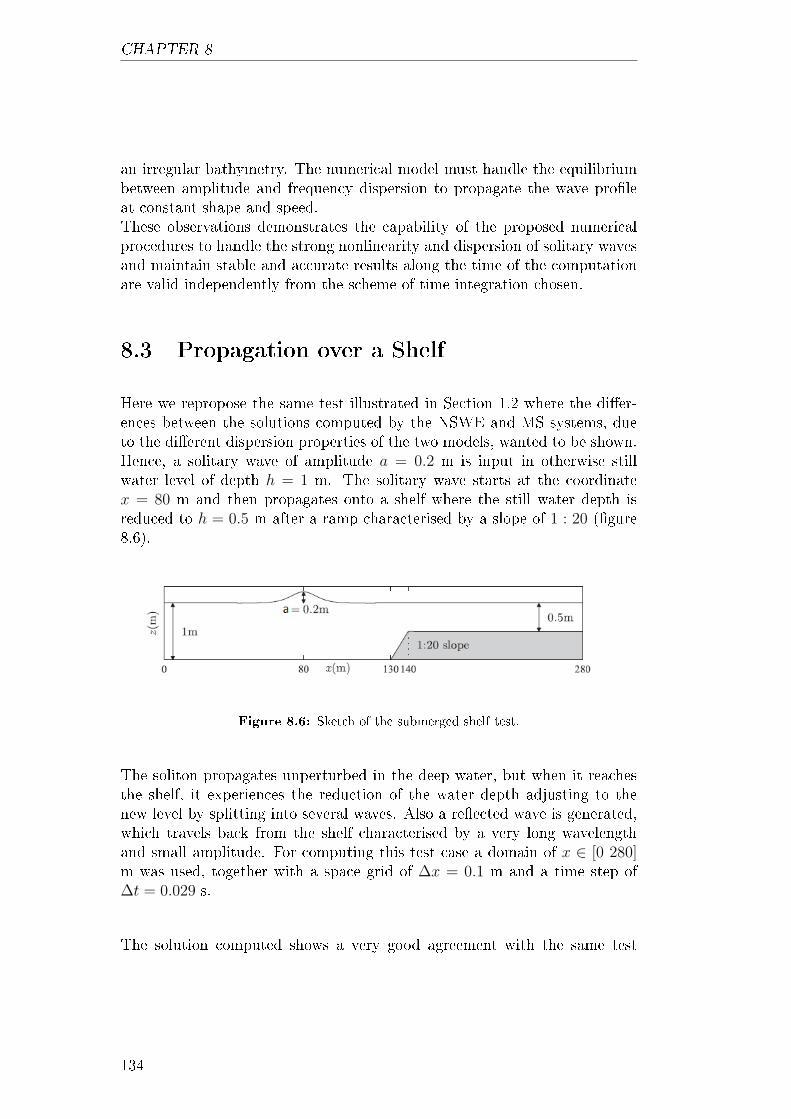
CHAPTER 8

an irregular bathymetry. The numerical model must handle the equilibriumbetween amplitude and frequency dispersion to propagate the wave proleat constant shape and speed.These observations demonstrates the capability of the proposed numericalprocedures to handle the strong nonlinearity and dispersion of solitary wavesand maintain stable and accurate results along the time of the computationare valid independently from the scheme of time integration chosen.

8.3 Propagation over a Shelf

Here we repropose the same test illustrated in Section 1.2 where the dier-ences between the solutions computed by the NSWE and MS systems, dueto the dierent dispersion properties of the two models, wanted to be shown.Hence, a solitary wave of amplitude a = 0.2 m is input in otherwise stillwater level of depth h = 1 m. The solitary wave starts at the coordinatex = 80 m and then propagates onto a shelf where the still water depth isreduced to h = 0.5 m after a ramp characterised by a slope of 1 : 20 (gure8.6).

Figure 8.6: Sketch of the submerged shelf test.

The soliton propagates unperturbed in the deep water, but when it reachesthe shelf, it experiences the reduction of the water depth adjusting to thenew level by splitting into several waves. Also a reected wave is generated,which travels back from the shelf characterised by a very long wavelengthand small amplitude. For computing this test case a domain of x ∈ [0 280]m was used, together with a space grid of ∆x = 0.1 m and a time step of∆t = 0.029 s.

The solution computed shows a very good agreement with the same test

134

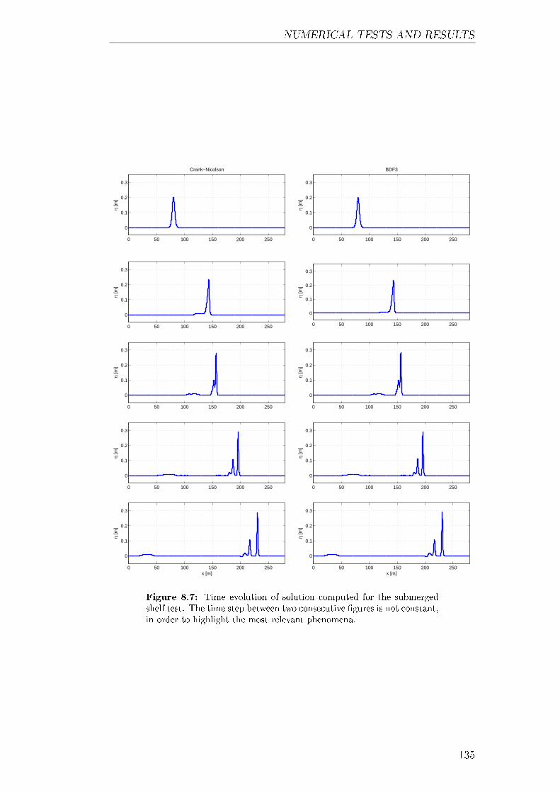
NUMERICAL TESTS AND RESULTS

0 50 100 150 200 250

0

0.1

0.2

0.3

Crank−Nicolson

η [m

]

0 50 100 150 200 250

0

0.1

0.2

0.3

BDF3

η [m

]

0 50 100 150 200 250

0

0.1

0.2

0.3

η [m

]

0 50 100 150 200 250

0

0.1

0.2

0.3

η [m

]

0 50 100 150 200 250

0

0.1

0.2

0.3

η [m

]

0 50 100 150 200 250

0

0.1

0.2

0.3

η [m

]

0 50 100 150 200 250

0

0.1

0.2

0.3

η [m

]

0 50 100 150 200 250

0

0.1

0.2

0.3

η [m

]

0 50 100 150 200 250

0

0.1

0.2

0.3

x [m]

η [m

]

0 50 100 150 200 250

0

0.1

0.2

0.3

x [m]

η [m

]

Figure 8.7: Time evolution of solution computed for the submergedshelf test. The time step between two consecutive gures is not constant,in order to highlight the most relevant phenomena.

135

CHAPTER 8

results reported in [21]. In gure 8.7 Crank-Nicolson and BDF3 time in-tegration of the SU/PG scheme can be compared. Both the solutions wellreproduces the wave propagation and transformation overall the domain.The eect of the bathymetry transforms the shape and slope of the soliton,increasing its amplitude and steepness and generating a train of secondarywaves of minor amplitude due to the dispersion. The input wave, in fact,which is able to travel unperturbed along the region of constant bathymetryh = 1 m, represents a stable solution for the Madsen-Sørensen system forthat conguration of the sea bottom, because it is obtained by directly inte-grating the system with the procedure explained in Section 7.1. When thebathymetry raise and the new bottom level is set to h = 0.5 m, the systemautomatically adjust the solution, under the conservation laws constraint,searching for a new stable solution over the new bathymetry conguration.The new soliton wave, which originates from this adjustment, represents anew stable solution, potentially recoverable using the procedure of Section7.1. In the transient of its formation, a dispersion of the slower frequenciestakes place. In Section 1.3.2 we have shown that the dispersion descriptiongiven by the Madsen and Sørensen system results in a k-dependent value ofthe phase velocity C(k). Hence, a train of waves takes form from the originalsolitary wave. Each of them originates from the wake that the one immediateforward left behind during its propagation at its own velocity.The phenomenon is well represented in the sequential representation of thetest in gure 8.7. The solitary wave, in fact, changing its shape becomes atrain of dierent waves. Each element of this dispersive wake travels with anown dierent speed; in the gure in fact we can see that the distant betweenthe several waves increase, such that a train of stable solitons results in theend.

Figure 8.8 compare the propagation and fragmentation of the solitary wavecomputed by the SU/PG scheme with CN time integration (a) with respectto the test results presented in [21] (b). The agreement between the twosolutions is very strong and is a symptom of the goodness of the schemeproposed in the representation of the high dispersive character of this test.

In the above gure 8.9, the results computed by the several schemes proposedin Chapter 3 and integrated in time with the CN method are compared. All ofthem give an accurate description of the physical aspect of the phenomenon.However, the dispersion analysis of the schemes described in Chapter 3, andriassumed by the gures 5.4 and 5.5, it is here conrmed by the zoom ingure 8.9(b). In the pictures, in fact, the dierence between the curves areprincipally due to the fact that the several schemes solved the dispersion

136

NUMERICAL TESTS AND RESULTS

(a)

(b)

Figure 8.8: Splitting of a solitary wave propagating over a submergedshelf: (a) numerical computation using SU/PG scheme with CN timeintegration; (b) test results presented in [21].

137

CHAPTER 8

0 50 100 150 200 250

0

0.1

0.2

0.3

x [m]

η [m

]

Central GalerkinCentral RDSU/PGU/RD

(a)

227 228 229 230 231 232 233 234−0.05

0

0.05

0.1

0.15

0.2

0.25

0.3

x [m]

η [m

]

Central GalerkinCentral RDSU/PGU/RD

(b)

Figure 8.9: Overlapping of the several results of the submerged shelftest, obtained integrating the dierent schemes with the CN method (a),and close-up of the peaks regions to highlight the dierence between thesolutions computed (b).

properties of the MS model with dierent levels of accuracy. This fact gener-ates the dierences in computing the amplitude and celerity of the solitons inthe transitory between the two bathymetry levels which create also the errorin phase. In particular, it can be see that the residual distribution schemesgive exactly the same result, conrming what was shown in gure 5.4 aboutthe equality of their dispersive properties. Between the Galerkin and theSU/PG curves, instead, not only the eect of a better dispersive descriptionexplains the dierences, but also the existence of an articial dissipation inthe SU/PG method which weakly decrease the soliton amplitude computed.

Figure 8.10, instead, shows the same comparison between the schemes whichare here integrated in time using the BDF3 method. The central Galerkinand RD schemes appear to be not stable for this choice of the grid space andtime step of the integration, and that is why in the gure only the curvesrelated to the upwind schemes are shown. The same consideration as beforebetween the dispersion properties of the two schemes can be done. Globally,the results only weakly diers from the ones computed using the other timeintegration method.

Looking to the strong deformation in amplitude and steepness experiencedby the waves in this test case, a more realistic description of the phenomenonshould contain a model able to individuate and manage the eventual genera-tion of shocks. This model, in fact, as largely explained in the introduction,

138

NUMERICAL TESTS AND RESULTS

0 50 100 150 200 250

0

0.1

0.2

0.3

x [m]

η [m

]

SU/PGU/RD

(a)

227 228 229 230 231 232 233 234−0.05

0

0.05

0.1

0.15

0.2

0.25

0.3

x [m]

η [m

]

SU/PGU/RD

(b)

Figure 8.10: Overlapping of the several results of the submerged shelftest, obtained integrating the dierent schemes with the BDF3 method(a), and close-up of the peaks regions to highlight the dierence betweenthe solutions computed (b).

is not able to described the wave breaking and a switch on the use of theshallow water model should be done for this purpose. The methods devel-oped in this work are robust even in the description of the NSWE model,hence, this could be one of the possible future advancement.

8.4 Periodic Wave Propagation over a Submerged

Bar

[39] described a series of laboratory experiments to investigate wave propaga-tion and dispersion over a submerged bar. The experimental data collectedcan be used here to validate the schemes proposed. In particular the ex-periment having the conguration shown in gure 8.11 is here presented.The test consists in a periodic wave of period T = 2.02 s and amplitudea = 0.01 m which propagates into an initially undisturbed region of depthbefore reaching a bar of the shape and proportions given in the gure.The numerical set for this test case needs the use of a periodic internal wavegenerator, like the one described in Section 7.3 and centred at the coordinatex = 10 m of the domain x ∈ [0 35] m. It is found that the wave generates bythis method has a dierent amplitude compared to the one expected, while

139

CHAPTER 8

instead the period and wavelength were described correctly. An accuratesetting of the parameters of the source function were done, which at the endallowed a more accurate representation of the periodic input wave will. Twosponge layers of the kind described in Section 7.2 are then used at the twoboundaries of the domain, extended on the regions x ∈ [0 3] m on the leftand x ∈ [32 35] m on the right, to absorb any wave reaching the boundaries.

Figure 8.11: Sketch of the computational conguration of the numer-ical test of the propagation over a submerged bar.

The comparison between numerical solution and the experimental data ismade up on the time histories of the free surface prole measured with gaugesin the positions denoted in gure 8.11 by the numbers 4, 5, 6, 7, 8, and 9and correspondent to the physical coordinates x4 = 20.5 m, x5 = 22.5 m,x6 = 23.5 m, x7 = 24.5 m, x8 = 25.7 m, and x9 = 27.3 m. The equations areintegrated using a grid size ∆x = 0.04 m and a time step ∆t = 0.0323. Thecomputational domain was made long enough in order to avoid any interfer-ence with reected waves that might be generated at the boundaries duringthe calculus.Figures 8.12 and 8.13 show the surface elevation of the sinusoidal wave trans-formation over the submerged bar. Each graphic of the two gures illustratesthe trend in time of the surface elevation on the experimental gauge posi-tion. In such a way numerical solutions and experimental data are directlycomparable on the various sections of the test.

140

NUMERICAL TESTS AND RESULTS

33 34 35 36 37 38 39−0.02

−0.01

0

0.01

0.02

0.03

0.04

η [m

]

x [m]

CN − gauge 4

33 34 35 36 37 38 39−0.02

−0.01

0

0.01

0.02

0.03

0.04

η [m

]

x [m]

BDF3 − gauge 4

33 34 35 36 37 38 39−0.02

−0.01

0

0.01

0.02

0.03

0.04

η [m

]

x [m]

gauge 5

33 34 35 36 37 38 39−0.02

−0.01

0

0.01

0.02

0.03

0.04

η [m

]

x [m]

gauge 5

33 34 35 36 37 38 39−0.02

−0.01

0

0.01

0.02

0.03

0.04

η [m

]

x [m]

gauge 6

33 34 35 36 37 38 39−0.02

−0.01

0

0.01

0.02

0.03

0.04η

[m]

x [m]

gauge 6

33 34 35 36 37 38 39−0.02

−0.01

0

0.01

0.02

0.03

0.04

η [m

]

Time [s]

gauge 7

33 34 35 36 37 38 39−0.02

−0.01

0

0.01

0.02

0.03

0.04

η [m

]

Time [s]

gauge 7

Figure 8.12: Time evolution at the gauges coordinates of the surfaceelevation of sinusoidal wave encountering a submerged bar, with initialamplitude a = 0.01 m and period T = 2.02 s. In gure, represents theexperimental data, is the central Galerkin, is the SU/PG and

is the U/RD scheme.

141

CHAPTER 8

33 34 35 36 37 38 39−0.02

−0.01

0

0.01

0.02

0.03

0.04

η [m

]

x [m]

CN − gauge 8

33 34 35 36 37 38 39−0.02

−0.01

0

0.01

0.02

0.03

0.04

η [m

]

x [m]

BDF3 − gauge 8

33 34 35 36 37 38 39−0.02

−0.01

0

0.01

0.02

0.03

0.04

η [m

]

x [m]

gauge 9

33 34 35 36 37 38 39−0.02

−0.01

0

0.01

0.02

0.03

0.04

η [m

]

x [m]

gauge 9

33 34 35 36 37 38 39−0.02

−0.01

0

0.01

0.02

0.03

0.04

η [m

]

Time [s]

gauge 10

33 34 35 36 37 38 39−0.02

−0.01

0

0.01

0.02

0.03

0.04

η [m

]

Time [s]

gauge 10

Figure 8.13: Time evolution at the gauges coordinates of the surfaceelevation of sinusoidal wave encountering a submerged bar, with initialamplitude a = 0.01 m and period T = 2.02 s. In gure, represents theexperimental data, is the central Galerkin, is the SU/PG and

is the U/RD scheme.

The schemes performed very well for all the gauges up to the crest of the bar(gauge 8), maintaining a good agreement with the experimental results andshowing only a weak error in the phase shift despite the strong nonlinearity;it should be noted that part of the discrepancies between the laboratory dataand the models results might be due to the experimental setup. In addition,very thin dierences appears between the solutions computed via the useof the BDF3 method, instead of the CN one and only the central residualdistribution scheme results surprisingly unstable for this particular choice ofintegration parameter for both the cases.However, as the waves pass the back slope of the bar, some discrepancies withthe data appear, especially at the section of gauge 10. This is due to theactivation of a numerical phenomenon which decoupled the higher harmonicsfrom the primary longer wave; these are released as free waves propagatinggenerating inaccuracy. The central Galerkin and the upwind residual distri-bution schemes appears to be more sensible to this kind of problems, while

142

the SU/PG one show a more robust trend with respect to them.This test case has provided a severe test of the models as nonlinearity hasinitially steepened the waves on the up-slope and then the increasing depthbehind the bar has decomposed the waves into short wave components. Thisresulted in a rapidly varying prole behind the bar with the exact form de-pending crucially on the dispersive characteristics of the numerical modelsanalysed. As expected from the theoretical limitations of the present MSmodel, some discrepancies show up as higher harmonics are released behindthe bar. Nevertheless the agreement is still quite reasonable and the dis-cretization schemes proposed for its integration showed the conservation andwell representation of the nonlinear and dispersive properties of the originalcontinuous model.

143

144

Conclusions

In this thesis the numerical approximation of nonlinear and dispersive ex-tended Boussinesq wave equations was considered. We have introduced inChapter 1 the problem of the numerical modelling of the wave propagationin the near-shore zone with the NSWE system and it was shown that thereis a variety of equation systems, termed Boussinesq-type, which give moreaccurate solutions to this problem and which can be compared by consider-ing their linear dispersion characteristics. A compromise has to be reachedbetween the theoretical accuracy of the mathematical model and the prac-ticalities of the numerical solution of the systems. In this work a system ofextended one-dimensional Boussinesq equations due to Madsen and Sørensenwas taken into account: its mathematical properties were compared to theoriginal Boussinesq system and it was shown that the MS equations weresignicantly more accurate.Weighted residuals numerical methods to discretize in space nonlinear anddispersive wave equations were introduced in Chapter 2 and then developedand implemented for the simpler cases of linear scalar advection and linearscalar advection with dispersion problems in the following Chapters 3 and4. In particular, nite dierence second and fourth order schemes were de-veloped in order to compare their accuracy and dispersion properties, withrespect to the ones of more complex nite element and residual distributionsschemes, implemented after. The nite dierence schemes was not consideredfurther due to the fact that only those discretization methods which could belater applied to unstructured two-dimensional meshes were of interest here.However, we have shown how those methods which use the same second orderreconstruction of the spatial derivatives can actually reach higher truncationerror orders, thank to particular coecients of the mass matrices and cangive more accurate approximations of the discretized model dispersion. Inparticular we have shown that the Galerkin nite element mass matrix givesto its central discretized scheme the best accuracy properties, up to the fourthorder in the scalar advection case, using the half of the stencil to accomplish

145

this, compare to the FD4 scheme.We have then introduced a way to stabilize the central Galerkin and RDschemes by means of a residual upwind term. We have shown that a partic-ular choice of the weighting functions which pre-multiply this term allows toobtain, in one case, a kind of streamline upwind Petrov-Galerkin scheme and,in the other case, an upwind residual distribution scheme. It has been shownthat the use of this technique in order to stabilize a central scheme does notaect the accuracy order of the centred part and that only in the SU/PGmethod some non-physical diusion is added to the model. The accuracyand the dispersive properties of all these spatially discretized schemes wereinvestigated and shown.The numerical solution of the full Madsen and Sørensen one-dimensional sys-tem was described in Chapter 5. It was shown that the methods presented inthe previous chapter could be directly applied to this case, using a techniqueto decrease the high derivative order of the system, by means of the intro-duction of one or in some cases two auxiliary variables: their role wasto assume the reconstructed values of the spatial derivatives of the originalvariable of the system, increasing the number of variables and the dimensionof the system. Even with this manipulation, the schemes maintained thesame properties underlined in the previous chapters.The techniques to spatially discretise the system of equations we dealt withgave as results a series of system of ODEs in time, which were integrated usingimplicit linear multistep methods of the second (CN ) and third (BDF3) or-der. In Chapter 6 the way to eciently implement these schemes is shown: asolution adopted to speed-up the calculation consisted of freezing the expres-sion of the Jacobian matrix of the Newton iteration cycle as long as possible,and recomputing it only when the error produced by its approximation ex-ceeds a given tolerance. The convergence study conrmed the expected bet-ter convergence trend for schemes using the BDF3 time integration, howeverthis appeared to be less stable, since in certain congurations of the grid size∆x and time step ∆t only the stabilized upwind methods could compute ac-curately the solution, conrming the goodness of the operated stabilisation.This behaviour is due to the lack of A-stability when the BDF3 integrationmethod is applied, in fact, all the schemes result stable if integrated by theCN method. In this case low CFL numbers are not needed for stability butionly for numerical accuracy.The numerical methods have been nally tested against theoretical and ex-perimental rusults in Chapter 8. Very good agreements were obtained, con-rming that the schemes proposed are able to solve highly nonlinear anddispersive problems with an high order of accuracy. Weak dierences emergeamong the results of the several used techniques, depending on their degree

146

of accuracy and expecially on their goodness to well reproduce the modeldispersion properties. In particular the residual distribution central and up-wind schemes appeared to provide a weakly worse description with respectto the more accurate one given by Galerkin based methods. In addition, theSU/PG scheme better represents the theoretical and experimental shape ofthe free surface, since it gives the best approximation of the original modeldispersion, being also more robust against instabilities which can arise whena higher order time integration method is used, instead of the second orderCN . For these reasons the SU/PG scheme appears to be the most promisingscheme with respect to the ones proposed and, since it is also suitable for theshallow water system solution [38], it is the best candidate to be developedfurther.

Future works : The integration methods proposed for the one-dimensionalMS system of extended Boussinesq equations are able to well solve the highlynonlinear and dispersive problem of the wave propagation over a variablebathymetry, giving an accurate description of the free surface water levelshape all over the computational one-dimensional domain, but the presentpreliminary results could originate a wide variety of developments and im-provements.In order to build a comprehensive method, capable of solving all the prop-agation phenomenon in the near-shore zones, both the management of themoving shoreline and a criteria useful to detect and well solve the breakingwave points have to be included. A possibility is the addition of articialviscosity to the original model (like in []). However the particular class ofdeveloped methods within this work is able to well solve also the NSWE too.In this way, a switch into the shallow water system, once the wave breakingis detected ([30]) would be easy to be implemented and is expected to givebetter results.High order models can be treated with the proposed methods, extendingthe range of applicability of the model here obtained by adding to the MSequations genuinely nonlinear dispersion terms ([7]) and dealng with theGreen-Naghdi system of equations.Other future works could regard the numerical implementation, with the useof the same techniques explained here, of the two-dimensional Madsen andSørensen problem. This was, in fact, one of the main purposes whereby thechoice of the discretization methods was made. In this huge eld, manyupgrades could be investigated and accomplished. In particular, adaptivedynamic meshes could be implemented in order to follow the wave fronts

147

and moving shorelines, giving them better reconstructions. By the numeri-cal point of view, higher order nite elements (P2 basis functions or hermitehierarchical nite elements or al.) could be used for the numerical approx-imation of the solution in space; higher order time handling (BDF typeintegration or space-time nite elements) could be tested. Finally, the par-allelization of the code could allow the computation over huge domains andlarge scale applications (e.g. several kilometres o shore).

148

Appendix A

Demonstration of the Equality 2.5

In Chapter 2 we use the integration by parts to transfer the spatial derivativefrom the discrete value of the ux fh to the weighting function of the weakformulation ϕi. This possibility is originated if fh ∈ C0 on each element'sclosure and fh ∈ C1 on the element itself, using the relation (2.5):

∫Ω

ϕi∂xfhdx = −∫

Ω

fh∂xϕidx (A.1)

In fact, given the particular linear form of the weighting functions on thecompact stencil [i− 1, i+ 1], represented in gure 2.1, the integral termextended over the whole domain Ω becomes an integral over the compactsupport of the weighting function:

−∫

Ω

fh∂xϕidx = −∫ i+1

i−1

fh∂xϕidx (A.2)

However, ∂xϕi is a discontinuous function in the interval [i−1, i+1], thus,in order to be computed, the integral in equation (A.2) must be partitionedin two over the discontinuity:

−∫

Ω

fh∂xϕidx = −∫ i

i−1

fh∂xϕidx−∫ i+1

i

fh∂xϕidx (A.3)

In this way the function ∂xϕi is now continuous over each the two intervals

149

[i−1, i] and [i, i+1]. Now using the property of the derivation of the productof functions, we have:

−∫ i

i−1

fh∂xϕidx = −∫ i

i−1

∂x (ϕifh) dx+

∫ i

i−1

ϕi∂xfhdx (A.4)

−∫ i+1

i

fh∂xϕidx = −∫ i+1

i

∂x (ϕifh) dx+

∫ i+1

i

ϕi∂xfhdx (A.5)

Recollecting the two expressions and solving some terms, we thus obtain:

−∫ i+1

i−1

fh∂xϕidx = (ϕifh) |i−1 − (ϕifh) |i +

∫ i

i−1

ϕi∂xfhdx+

+ (ϕifh) |i − (ϕifh) |i+1 +

∫ i+1

i

ϕi∂xfhdx

(A.6)

Simplifying some terms and remembering that the weighting function ϕi isidentically null when evaluated in nodes i+1 and i−1 (see gure 2.1), thenal expression states:

−∫

Ω

∂xϕifhdx =

∫ i

i−1

ϕi∂xfhdx+

∫ i+1

i

ϕi∂xfhdx = (A.7)

=

∫Ω

ϕi∂xfhdx

which demonstrate that it is possible, under the initial hypotheses of conti-nuity of the function fh and about form of the basis functions ϕi, to exchangethe spatial derivative between the two functions through the only change ofthe sign of the integral.

150

Appendix B

Auxiliary Variables Choice for the

Linear Advection-Dispersion

Problem

We want to introduce an auxiliary variable w in order to reduce the order ofthe dispersive term of the linear advection with dispersion partial dierentialequation. The possibilities are to reconstruct separately the rst or secondorder spatial derivative contained in this term and then coupled this recon-struction with the modied equation of the problem. In this appendix itwill be shown that the two choices lead to the same nite dierence approx-imation of the term −α∂xxtu of the equation (4.1) and are, thus, completelyequivalent in this case.We can thus dene two auxiliary variables w1 and w2 which will assume theexpressions:

w1,i = ∂xui (B.1)

w2,i = ∂xxui (B.2)

The dierent choices lead to the two dierent residual formulations of thedispersive term −α∂xxt listed below:

151

−∫

Ω

ωiα∂xtw1,idx (B.3)

−∫

Ω

ωiα∂tw2,idx (B.4)

If P1 weighting functions of the kind of the Galerkin nite element schemeare chosen, solving the denite integrals on the spatial domain using themiddle point quadrature rule, since a residual distribution form for this termsis searched, the results will be:

− α

2(dw1,i+1

dt− dw1,i−1

dt) (B.5)

− α∆x

4(dw2,i+1

dt+ 2

dw2,i

dt+dw2,i−1

dt) (B.6)

Equation (B.1) and (B.2) must be discretized too and, being part of a cou-pled system with the advection-dispersion equation, they are going to beintegrated in the domain used the same middle point rule. This will lead tothe expression:

∆x

4w1,i−1 +

∆x

2w1,i +

∆x

4w1,i+1 =

1

2∆x(ui+1 − ui−1) (B.7)

∆x

4w2,i−1 +

∆x

2w2,i +

∆x

4w2,i+1 =

1

∆x2(ui+1 − 2ui + ui−1) (B.8)

The mass lumping technique can be use on equations (B.7) and (B.8), ob-taining for the auxiliary variables w1 and w2 the second order nite dierenceapproximation respectively of the rst and second order derivative:

w1,i =1

2∆x(ui+1 − ui−1) (B.9)

w2,i =1

∆x2(ui+1 − 2ui + ui−1) (B.10)

Using (B.9) and (B.10) to compute the values of the auxiliary variables in thei+1, i and i−1 nodes of the mesh, substituting their expression into (B.5) and

152

(B.6), the equality between the two approaches is demonstrate since both thetwo expression approximate the dispersive term of the equation (4.1) throughthe form:

− α

4∆x(dui+2

dt− 2

duidt

+dui−2

dt) (B.11)

which, with respect to the second order nite dierence approximation (4.5),enlarges the stencil of the scheme.

153

Appendix C

Space-Discretization of the

Linearized MS System

In this Appendix, the several semi-descrete schemes, derived in Chapter 5for the MS systems of equations and shown in Appendix, are applyed on thesimpler linearised case under the assumption of constant bathymetry h = h0.We have already shown the form of this model in the Section 1.3.2, but forconvenience it is rewritten in the following:

∂tη + h0∂xu = 0

∂tu−Bh20∂xxtu+ g∂xη − βgh2

0∂xxxη = 0(C.1)

FD2 : The FD2 scheme is obtained simply applying the second orderaccuracy nite dierent approximation of the spatial derivatives present inthe two equations of the system. The nal expression of the scheme obtainedis thus:

155

dηidt

+h0

2∆x(ui+1 − ui−1) = 0 (C.2)

duidt− Bh2

0

∆x2

(dui−1

dt− 2

duidt

+dui+1

dt

)+

+g

2∆x(ηi+1 − ηi−1) +

− β gh30

2∆x2(−ηi−2 + 2ηi−1 − 2ηi+1 + ηi+2) = 0

FD4 : Similarly, approximating the spatial derivatives using the fourthorder nite dierence formulae, instead of the second ones, the FD4 schemewill result:

dηidt

+h0

12∆x(ui−2 − 8ui−1 + 8ui+1 − ui+2) = 0 (C.3)

duidt− Bh2

0

12∆x2

(−dui−2

dt+ 16

dui−1

dt− 30

duidt

+ 16dui+1

dt− dui+2

dt

)+

+g

12∆x(ηi−2 − 8ηi−1 + 8ηi+1 − ηi+2) +

− β gh30

8∆x2(ηi−3 − 8ηi−2 + 13ηi−1 − 13ηi+1 + 8ηi+2 − ηi+3) = 0

Galerkin nite element : In the following the system (C.1) is spatiallydiscretized with the central Galerkin nite element method discussed in Sec-tion 5.2. The auxiliary variable w is the same dened by (5.17) and thescheme results in:

∆x

6

dηi−1

dt+

2∆x

3

dηidt

+∆x

6

dηi+1

dt+h0

2(ui+1 − ui−1) = 0 (C.4)

∆x

6

dui−1

dt+

2∆x

3

duidt

+∆x

6

dui+1

dt+g

2(ηi+1 − ηi−1) +

− Bh20

∆x

(dui−1

dt− 2

duidt

+dui+1

dt

)+

− β gh20

2∆x2(−ηi−2 + 2ηi−1 − 2ηi+1 + ηi+2) = 0

(C.5)

156

Central Residual Distribution : In Section 5.3 the development of acentral residual distribution scheme for the system of MS non-hydrostaticequations is proposed and discussed. It resulted in the system of four PDEs(5.41). The same form of the system is still valid in the linearised case, theexpressions of the residual uxes ΦK

η and ΦKq , however, must be rewritten.

First of all the residual ux ΦKq becomes ΦK

u in the linearised case since thevariable q is no more present in system (C.1), but the only u remains. As aconsequence, also the auxiliary variable wq, is here introduced with the sameexpression of (5.36) for the reconstruction of the second space derivative ofthe velocity u.Then, taking into account the cell formed by the nodes i and i−1, we canderive the following form of the residuals:

Φi− 1

2η = ∆x

dηi− 12

dt+ h0 (ui − ui−1)

Φi− 1

2u = ∆x

dui− 12

dt−∆xBh2

0

dwu,i− 12

dt+

+ g (ηi − ηi−1)− βgh20 (wη,i − wη,i−1)

(C.6)

with which the central residual distribution scheme for the linearised problemcan than be written in the same form of (5.41).

Stabilized Upwind schemes : The general form of the streamline upwindschemes, derived computing the sign of the local Jacobian matrix of therelative shallow water system, was given in (5.49). It was characterised bythe adding of a stabilisation term, based on the value of the residual uxesΦKη and ΦK

q , to a chosen CS (centred scheme). The expression of these uxeswas there computed using denitions (5.34) and (5.38).In the linearised context, the Jacobian matrix of the linear shallow watersystem assumes the simpler form (1.3.1), being, thus, constant in all thedomain since also the bathymetry h0 is assumed to be constant. Hence, thecomputation of sign(A) through the (5.50) results in:

sign(A) =

[0 c/gg/c 0

](C.7)

and (C.7) gives to (5.49) the simpler form:

157

[CSηCSu

]+

c

2g

[Φi− 1

2u

Φi− 1

2η

]− g

2c

[Φi+ 1

2u

Φi+ 1

2η

](C.8)

where the formulae (C.6) are used to compute the residual uxes ΦKη and

ΦKu of the upwind terms, which are then add to a central Galerkin or RD

spatial discretization of the linear system (C.1).

158

Appendix D

Auxiliary Variables Choice in the

MS Dispersion Term

Discretization

The discretization of the Madsen and Sørensen system of equations leads todeal with a third order spatial derivative term. When the use of Galerkinnite element discretization is requested and the use of P1 basis and weight-ing functions is preferred, the need of an auxiliary variable denition arises inorder to decrease the derivation order of this term. Exactly as in AppendixC two possible reconstructions can be adopted:

wη1,i = ∂xηi (D.1)

wη2,i = ∂xxηi (D.2)

Applying these dierent reconstructions to the weak formulation of the thirdderivative term, in the two cases it assumes the form:

βg

∫Ω

∂x(ϕih

3)∂xwη1,idx (D.3)

βg

∫Ω

∂x(ϕih

3)wη2,idx (D.4)

When the hypothesis of a constant bathymetry is done, hence h(x) = h0 =

159

const, the solution of these integrals leads to the following expressions:

βgh3

0

∆x(wη1,i+1 − 2wη1,i + wη1,i−1) (D.5)

βgh3

0

2(wη2,i+1 − wη2,i−1) (D.6)

In order to compute the values of the variables wη,i, which must be substitutein (D.5) and (D.6), the denitions of wη1 and wη2 need to be written in theweak formulation too and then integrated over the domain. This procedure,followed by the use of the mass lumping technique, allows to obtain for thevariables wη1,i and wη2,i analogous expressions to that in equations (B.9) and(B.10).The values of these auxiliary variable can, now, be computed in the i+1,iand i−1 nodes of the grid and substitute in (D.5) and (D.6). Analyticaldevelopment leads both the expression to be identically equal to:

βgh3

0

2∆x2(ηi+2 − 2ηi+1 + 2ηi−1 − ηi−2) (D.7)

which simply reects the second order nite dierence discretization of thethird order spatial derivative (see (5.3)) integrated over the domain.In conclusion, under the hypothesis of h = const the two dierent recon-structions leads to the same nal discretised expression of the third spatialderivative term ∂x3η. In cases in which this hypothesis results no more ver-ied, a small dierence in the two approaches originates in dependence onthe quadrature formula used to solve the denite integrals (D.3) and (D.4),but it seems not to aect the goodness of the solution.

160

Appendix E

Galerkin Space-Discretization of

the MS System

In Section 5.2 the Madsen and Sørensen system has been semi-discretized inspace developing a central Galerkin nite element method, using linear basisfunction and through the introduction of an auxiliary variable wη in orderdecrease the spatial derivation order of the system. The resulting scheme, inthe case of the complete nonlinear MS system and with variable bathymetryh(x), is listed below:

161

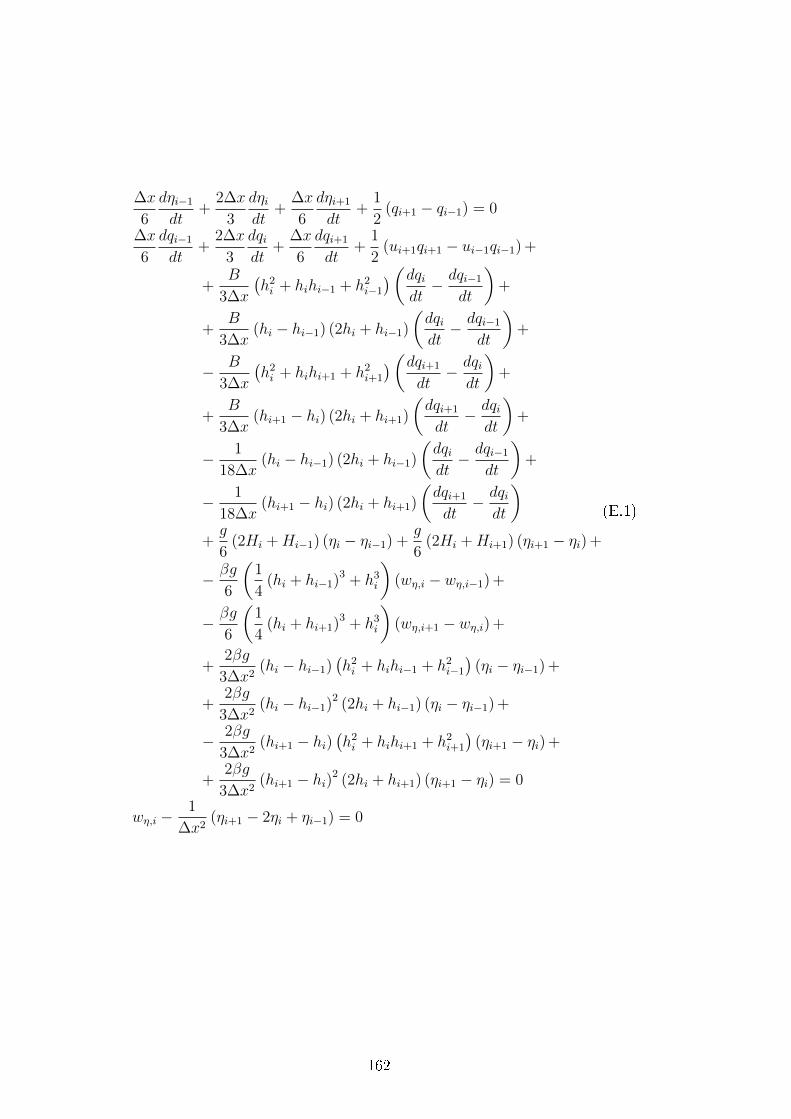
∆x

6

dηi−1

dt+

2∆x

3

dηidt

+∆x

6

dηi+1

dt+

1

2(qi+1 − qi−1) = 0

∆x

6

dqi−1

dt+

2∆x

3

dqidt

+∆x

6

dqi+1

dt+

1

2(ui+1qi+1 − ui−1qi−1) +

+B

3∆x

(h2i + hihi−1 + h2

i−1

)(dqidt− dqi−1

dt

)+

+B

3∆x(hi − hi−1) (2hi + hi−1)

(dqidt− dqi−1

dt

)+

− B

3∆x

(h2i + hihi+1 + h2

i+1

)(dqi+1

dt− dqi

dt

)+

+B

3∆x(hi+1 − hi) (2hi + hi+1)

(dqi+1

dt− dqi

dt

)+

− 1

18∆x(hi − hi−1) (2hi + hi−1)

(dqidt− dqi−1

dt

)+

− 1

18∆x(hi+1 − hi) (2hi + hi+1)

(dqi+1

dt− dqi

dt

)+g

6(2Hi +Hi−1) (ηi − ηi−1) +

g

6(2Hi +Hi+1) (ηi+1 − ηi) +

− βg

6

(1

4(hi + hi−1)3 + h3

i

)(wη,i − wη,i−1) +

− βg

6

(1

4(hi + hi+1)3 + h3

i

)(wη,i+1 − wη,i) +

+2βg

3∆x2(hi − hi−1)

(h2i + hihi−1 + h2

i−1

)(ηi − ηi−1) +

+2βg

3∆x2(hi − hi−1)2 (2hi + hi−1) (ηi − ηi−1) +

− 2βg

3∆x2(hi+1 − hi)

(h2i + hihi+1 + h2

i+1

)(ηi+1 − ηi) +

+2βg

3∆x2(hi+1 − hi)2 (2hi + hi+1) (ηi+1 − ηi) = 0

wη,i −1

∆x2(ηi+1 − 2ηi + ηi−1) = 0

(E.1)

162

Appendix F

Space-Time Discretization of the

Linearized MS System

This Appendix was created to show the fully expressions obtained integrat-ing with the Crank-Nicolson method the semi-discrete schemes illustrated inAppendix C. The resulted expressions written in the following are, thus, anumerical approximation of the linearised MS system (C.1) and they wereused in Section 6.1.1 in order to accomplish the study of the properties ofthe more complex schemes applied to the complete nonlinear Madsen andSørensen system (1.9).

Galerkin FE scheme with CN time integration : The system of space-time discretized equation, written below, is obtained rst spatially discretiz-ing the linearized version of the MS system of equation with the Galerkinnite element scheme of Section 5.2, then integrating the results with theCrank-Nicolson method explained in Section 6.1. The nal expression isthen related to a generic inner node i of the grid, to obtain:

163

1

6∆t

(ηn+1i−1 − ηni−1

)+

2

3∆t

(ηn+1i − ηni

)+

1

6∆t

(ηn+1i+1 − ηni+1

)+

+h0

4∆x

(un+ 1

2i+1 − u

n+ 12

i−1

)= 0

1

6∆t

(un+1i−1 − uni−1

)+

2

3∆t

(un+1i − uni

)+

1

6∆t

(un+1i+1 − uni+1

)+

− Bh20

∆t∆x2

((un+1i+1 − uni+1

)− 2

(un+1i − uni

)+(un+1i−1 − uni−1

))+

+g

4∆x

(ηn+ 1

2i+1 − η

n+ 12

i−1

)− βgh2

0

4∆x3

(wn+ 1

2η,i+1 − w

n+ 12

η,i−1

)= 0

(F.1)

The denition of the variable wη is coherent to what set all along this work.

RD scheme with CN time integration : In the residual distributionenvironment, the general form of the scheme remains the system of the fourPDEs (5.41), but the denitions of the residual uxes ΦK are, for instance:

Φi− 1

2η =

1

2∆t

(ηn+1i− 1

2

− ηni− 1

2

)+

h0

2∆x(ui − ui−1)n+1 +

h0

2∆x(ui − ui−1)n

Φi− 1

2u =

1

2∆t

(un+1i− 1

2

− uni− 1

2

)− Bh2

0

∆t

(wn+1u,i− 1

2

− wnu,i− 1

2

)+

+g

2∆x(ηi − ηi−1)n+1 +

g

2∆x(ηi − ηi−1)n +

− βgh20

2∆x(wη,i − wη,i−1)n+1 − βgh2

0

2∆x(wη,i − wη,i−1)n

(F.2)

Stabilization Upwind schemes with CN time integration : In Ap-pendix C a general form of the two stabilized upwind schemes developed inthis work is given trough (C.8). In the previous we have already explained, infact, that the dierence between the, what are here called, SU/PG methodand U/RD method regards the only choice of the centred scheme which ischosen to stabilized. We have shown, in fact, that the discretisazion of theupwind term leads in each case to the same result (if, of course, the samechoice of the auxiliary variables introduce in the system would be alwayscoherent with the what is here chosen).

164

Applying the Crank-Nicolson method to integrate in time the system (C.8),leads to the nal expression of the stabilized space-time discrete schemes. Inorder to generalized these expression, they can be still rewritten in the sameform of (C.8):

[CSηCSu

]+

c

2g

[Φi− 1

2u

Φi− 1

2η

]− g

2c

[Φi+ 1

2u

Φi+ 1

2η

](F.3)

However, even if (F.3) is formally equals to (C.8), the two context to whichthey belong make them deeply dierent. Here, in fact, the upwind term iscomputed with the expressions of the residuals ΦK

η and ΦKu given in (F.2).

The development of a SU/PG space-time discrete scheme for the linearisedMS system can than be reach replacing the term CS with the central Galerkinspace-time discrete scheme (F.1). On the other hand, the choice of a centredresidual distribution schemes using the same form of the residual uxes (F.2)leads to a U/RD space-discrete scheme.

[24]

165

166

Bibliography

[1] M. Kazolea A.I. Delis. Finite volume simulations of waves formed bysliding masses. Communications in numerical methods in engineering,27, 732-735, 2011.

[2] D. Ambrosi. Approximation of shallow water equations by roe's rie-mann solver. International Journal for numerical methods in uids, 20,157-168, 1995.

[3] H.B. Bingham T. Warburton A.P. Engsig-Karupp, J.S. Hesthaven. Dg-fem solution for nonlinear wave-structure interaction using boussinesq-type equations. Coastal Engineering, 55, 197, 2008.

[4] E. Audusse and M.-O. Bristeau. A well-balanced positivity preservingsecond-order scheme for shallow water ows on unstructured meshes.Journal of Computational Physics, 206(1):311 333, 2005.

[5] M. Behr. Stability anlysis of scalar advection-diusion equation.http://www.cats.rwth-aachen.de/library/research/technotes.

[6] A. Bermudez and M.E. Vazquez. Upwind methods for hyperbolic con-servation laws with source terms. Computers & Fluids, 23(8):1049 1071, 1994.

[7] P. Bonneton, E. Barthelemy, F. Chazel, R. Cienfuegos, D. Lannes,F. Marche, and M. Tissier. Recent advances in serre-green naghdi mod-elling for wave transformation, breaking and runup processes. EuropeanJournal of Mechanics - B/Fluids, In Press, Corrected Proof:, 2011.

[8] P. Brufau and P. Garcia-Navarro. Unsteady free surface ow simulationover complex topography with a multidimensional upwind technique.Journal of Computational Physics, 186(2):503 526, 2003.

167

[9] S.J. Sherwin C. Eskilsson. Spectral/hp discontinuous galerkin methodsfor modelling 2d boussinsq equations. Journal of Computational Physics210, 566, 2006.

[10] L. Quartapelle D. Ambrosi. A taylor-galerkin method for simulatingnonlinear dispersive water waves. Journal of computational physics,146, 546-569, 1998.

[11] P.A. Madsen D.R. Fuhrman. Simulation of nonlinear wave run-up witha high order boussinesq model. Coastal Engineering 55, 139, 2008.

[12] A. Ern and J.-C. Guermond. Theory and practice of nite elements,volume 159 of Applied Mathematical Sciences. Springer, 2004.

[13] A. Ern, S. Piperno, and K. Djadel. A well-balanced rungekutta discon-tinuous galerkin method for the shallow-water equations with oodingand drying. Int. J. for Numerical Methods in Fluids, 58(1):125, 2008.

[14] G.j. Fix G. Strang. an analysis of the nite element method. Prantice-Hall, 1973.

[15] J.T. Kirby G. Wei. A time-dependent numerical code for extendedboussinesq equations. Journal of Waterway, Port, Coastal, and OceanEngineering 120, 251-261, 1995.

[16] P. Garcia-Navarro, M. Hubbard, and A. Priestley. Genuinely multi-dimensional upwinding for the 2D shallow water equations. J. Comp.Phys., 121(1):7993, 1995.

[17] G. Hauke. A symmetric formulation for computing transient shallowwater ows. Computer Methods in Applied Mechanics and Engineering,163(1-4):111122, 1998.

[18] M. Hubbard and M.J. Baines. Conservative multidimensional upwindingfor the steady two-dimensional shallow-water equations. J. Comput.Phys., 138:419448, 1997.

[19] T.J.R. Hughes and M. Mallet. A new nite element formulation for CFDIII: the generalized streamline operator for multidimensional advective-diusive systems. Comp. Meth. Appl. Mech. Engrg., 58:305328, 1986.

[20] T.J.R. Hughes and T.E. Tezduyar. Development of time-accurate niteelement techniques for rst order hyperbolic systems with emphasys onthe compressible euler equations. Comp. Meth. Appl. Mech. Engrg.,45(1-3):217284, 1984.

168

[21] P.H. Taylor J. Orszaghova, A.G.L. Borthwick. From the paddle to thebeach - a bousinesq shallow water numerical wave tank based on mad-sen and sørensen's equations. Journal of Computational Physics, 231,328-344, 2012.

[22] J.F.T. Pittman J. Petera. Isoparametric hermite elements. Internationaljournal for numerical methods in engineering, 37, 3489-3519, 1994.

[23] J.T. Kirby. Boussinesq models and applications to near-shore wave prop-agation, surf zone processes and wave-induced currents. Advances inCoastal Modelling, 67, 1-41, 2003.

[24] A. Kurganov and E. Tadmor. Solution of two-dimensional Riemannproblems without Riemann solvers. Numerical Methods for PartialDierential Equations, 18:548608, 2002.

[25] D. Lannes and P. Bonneton. Derivation of asymptotic two-dimensionaltime-dependent equations for surface water wave propagation. Physicsof Fluids, 21, 2009. 016601 doi:10.1063/1.3053183.

[26] R. LeVeque. Finite volume methods for hyperbolic problems. Cam-bridge, 2002.

[27] R.J. LeVeque. Balancing source terms and ux gradients in high-resolution godunov methods: the quasi-steady wave-propagation algo-rithm. J. Comput. Phys., 146(1):346365, 1998.

[28] I.K. Nikolos C.E. Synolakis M. Kazolea, A.I. Delis. An unstructurednite volume numerical scheme for extended 2d boussinesq-type equa-tions. Coastal Engineering 69, 42-66, 2012.

[29] M. Petti M. Tonelli. Hybrid nite volume - nite dierence scheme for2dh improved boussinesq equations. Coastal Engineering, 56, 609-620,2009.

[30] F. Marche, P. Bonneton, P. Fabrie, and N. Seguin. Evaluation of well-balanced bore-capturing schemes for 2D wetting and drying processes.Int. J. Numer. Meth. Fluids, 53:867894, 2007.

[31] I.K. Nikolos and A.I. Delis. An unstructured node-centered nite vol-ume scheme for shallow water ows with wet/dry fronts over complextopography. Computer Methods in Applied Mechanics and Engineering,198(47-48):3723 3750, 2009.

169

[32] O. Nwogu. An alternative form of the boussinesq equations for near-shore wave propagation. Journal of Waterway, Port, Coastal, and OceanEngineering 119, 618-638, 1994.

[33] L. Sø rensen O.R. Sø rensen, H. Shaer. Boussinesq-type modellingusing an unstructured nite element technique. Coastal Engineering,50, 182, 2004.

[34] H. Liu P.A. Madsen, H. Bingham. A new boussinesq method for fullynonlinear waves from shallow to deep water. Journal of Fluid Mechanics462, 1, 2002.

[35] O.R. Sø rensen P.A. Madsen. A new form of the boussinesq equationswith improved linear dispersion characteristics. part 2: a slowing varyingbathymetry. Coastal Engineering 18, 183-204, 1992.

[36] M. Ricchiuto. Contributions to the development of residual discretiza-tion for hyperbolic conservation laws with applications to shallow waterows. HDR Thesis, University of Bordeaux, 2011.

[37] M. Ricchiuto, R. Abgrall, and H. Deconinck. Application of conserva-tive residual distribution schemes to the solution of the shallow waterequations on unstructured meshes,. J. Comput. Phys., 222:287331,2007.

[38] M. Ricchiuto and A. Bollermann. Stabilized residual distribution forshallow water simulations. J. Comput. Phys, 228(4):10711115, 2009.

[39] J.A. Battjes S. Beji. Numerical simulations of nonlinear-wave propaga-tion over a bar. Coastal Engineering, 23, 1-16, 1994.

[40] K. Nadoka S. Beji. A formal derivation and numerical modelling of theimproved boussinesq equations for varying depth. Ocean Engineering23, 691, 1996.

[41] R. Volker. Boussinesq-type model for near-shore wave processes in fring-ing reef environment. PhD Thesis, University of Hawaii and Manoa,2010.

[42] M.A. Walkley. A numerical method for extended boussinesq shallow-water wave equations. PhD Thesis, University of Leeds, 1999.

[43] Y. Xing and C.-W. Shu. High-order nite volume weno schemes for theshallow water equations with dry states. Advances in Water Resources,34(8):1026 1038, 2011.

170

[44] Y. Xing, X. Zhang, and C.-W. Shu. Positivity-preserving high order well-balanced discontinuous galerkin methods for the shallow water equa-tions. Advances in Water Resources, 33(12):1476 1493, 2010.

[45] Y.X. Yu G. Lai... Y.S. Li, S.X. Liu. Numerical modelling of boussinesqequations by nite element method. Coastal Engineering 37, 97, 1999.

171