35 - 1

Poisson Delaunay triangulation

35 - 2

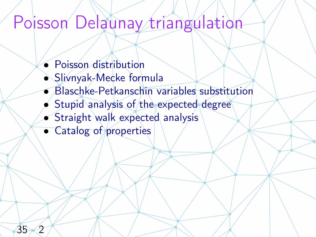
Poisson Delaunay triangulation

• Poisson distribution• Slivnyak-Mecke formula• Blaschke-Petkanschin variables substitution• Stupid analysis of the expected degree• Straight walk expected analysis• Catalog of properties

36 - 1

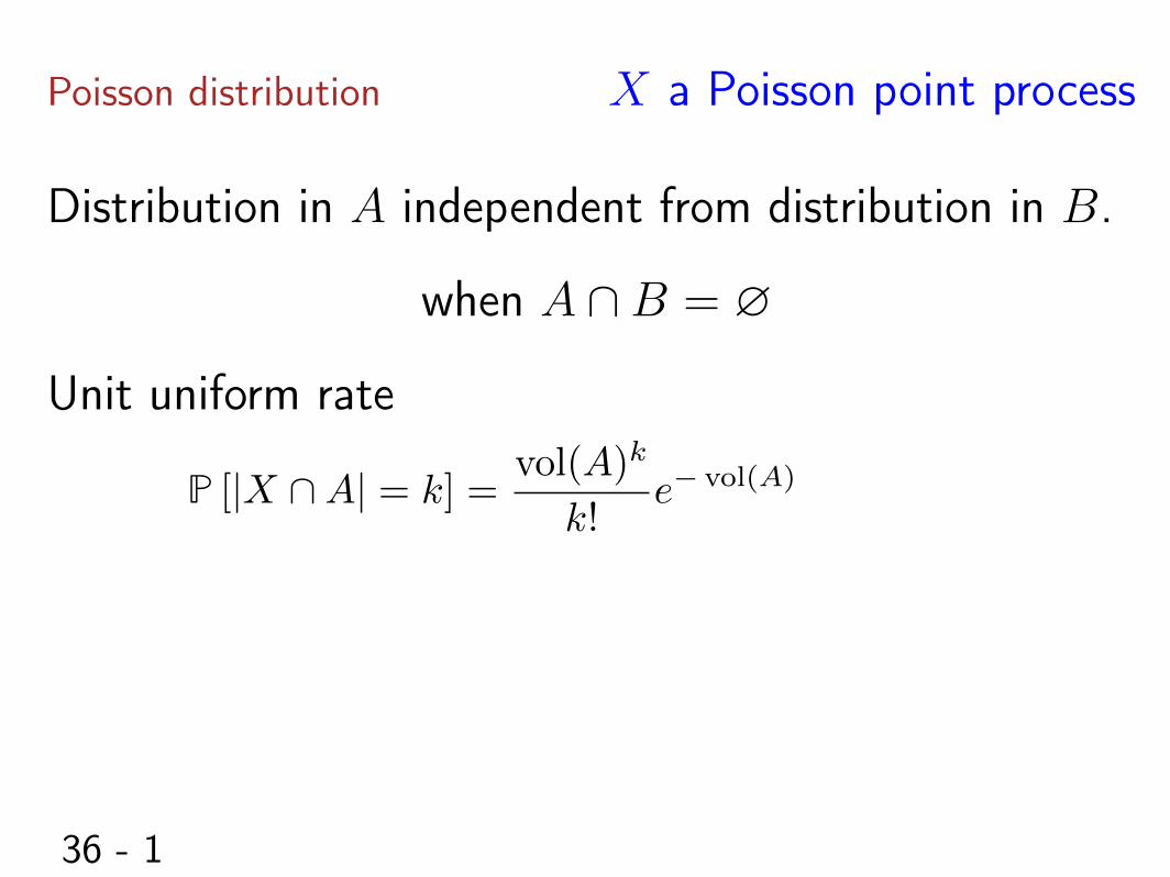
Poisson distribution

Distribution in A independent from distribution in B.

Unit uniform rate

when A \ B = ?

P [|X \A| = k] =vol(A)

k

k!e� vol(A)

X a Poisson point process

36 - 2

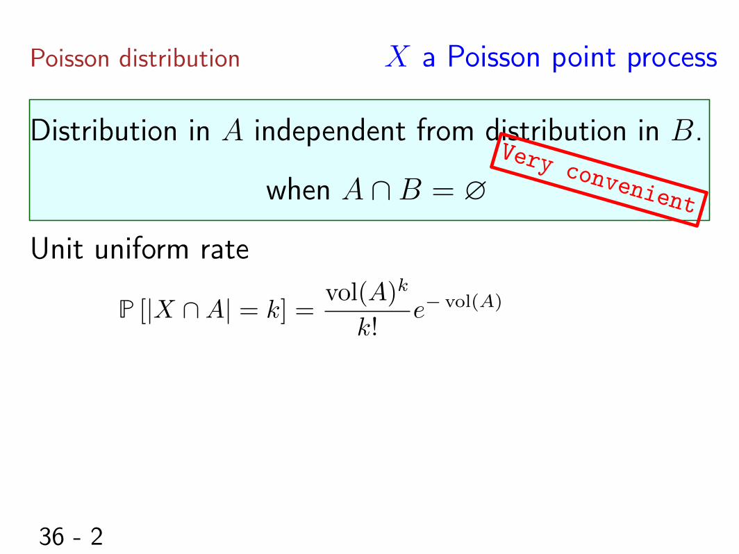
Poisson distribution

Distribution in A independent from distribution in B.

Unit uniform rate

when A \ B = ?

P [|X \A| = k] =vol(A)

k

k!e� vol(A)

V

e

r

y

c

o

n

v

e

n

i

e

n

t

X a Poisson point process

36 - 3

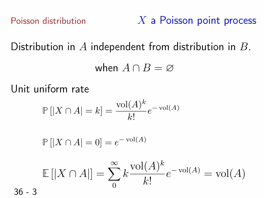
Poisson distribution

Distribution in A independent from distribution in B.

Unit uniform rate

when A \ B = ?

P [|X \A| = k] =vol(A)

k

k!e� vol(A)

E [|X \ A|] =1X

0

kvol(A)k

k!e� vol(A)

= vol(A)

P [|X \A| = 0] = e� vol(A)

X a Poisson point process

37 - 1

Slivnyak-Mecke formulaX a Poisson point process of density n

Sum Integral

37 - 2

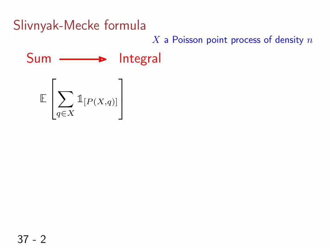
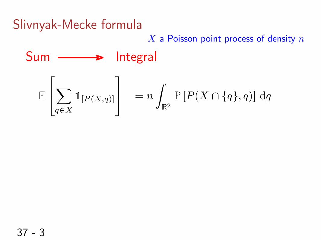
Slivnyak-Mecke formulaX a Poisson point process of density n

Sum Integral

E

2

4X

q2X

1[P (X,q)]

3

5

37 - 3

Slivnyak-Mecke formulaX a Poisson point process of density n

Sum Integral

E

2

4X

q2X

1[P (X,q)]

3

5= n

Z

R2

P [P (X \ {q}, q)] dq

37 - 4

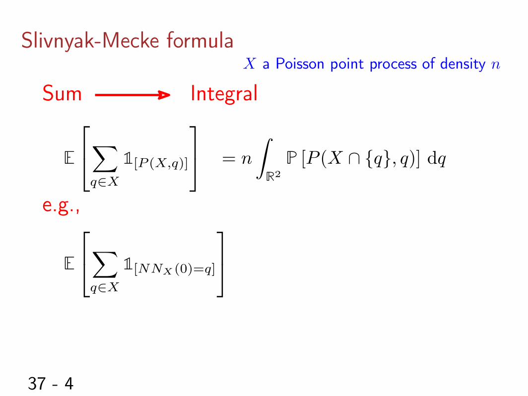
Slivnyak-Mecke formulaX a Poisson point process of density n

Sum Integral

E

2

4X

q2X

1[P (X,q)]

3

5= n

Z

R2

P [P (X \ {q}, q)] dq

e.g.,

E

2

4X

q2X

1[NNX(0)=q]

3

5

37 - 5

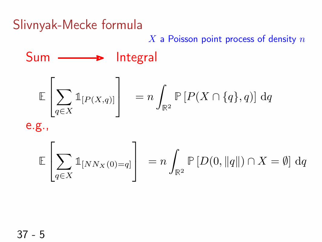
Slivnyak-Mecke formulaX a Poisson point process of density n

Sum Integral

E

2

4X

q2X

1[P (X,q)]

3

5= n

Z

R2

P [P (X \ {q}, q)] dq

e.g.,

E

2

4X

q2X

1[NNX(0)=q]

3

5= n

Z

R2

P [D(0, kqk) \X = ;] dq

37 - 6

Slivnyak-Mecke formulaX a Poisson point process of density n

Sum Integral

E

2

4X

q2X

1[P (X,q)]

3

5= n

Z

R2

P [P (X \ {q}, q)] dq

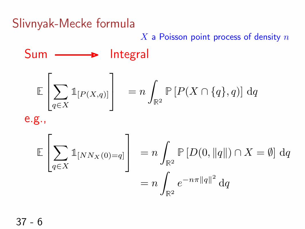
e.g.,

E

2

4X

q2X

1[NNX(0)=q]

3

5= n

Z

R2

P [D(0, kqk) \X = ;] dq

= n

Z

R2

e�n⇡kqk2

dq

37 - 7

Slivnyak-Mecke formulaX a Poisson point process of density n

Sum Integral

E

2

4X

q2X

1[P (X,q)]

3

5= n

Z

R2

P [P (X \ {q}, q)] dq

e.g.,

E

2

4X

q2X

1[NNX(0)=q]

3

5= n

Z

R2

P [D(0, kqk) \X = ;] dq

= n

Z

R2

e�n⇡kqk2

dq

= n

Z2⇡

0

Z 1

0

e�n⇡r2rd✓ dr = n⇥ 2⇡ ⇥ 1

2n⇡ = 1

38 - 1

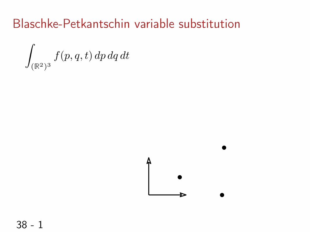
Blaschke-Petkantschin variable substitutionZ

(R2)

3

f(p, q, t) dp dq dt

38 - 2

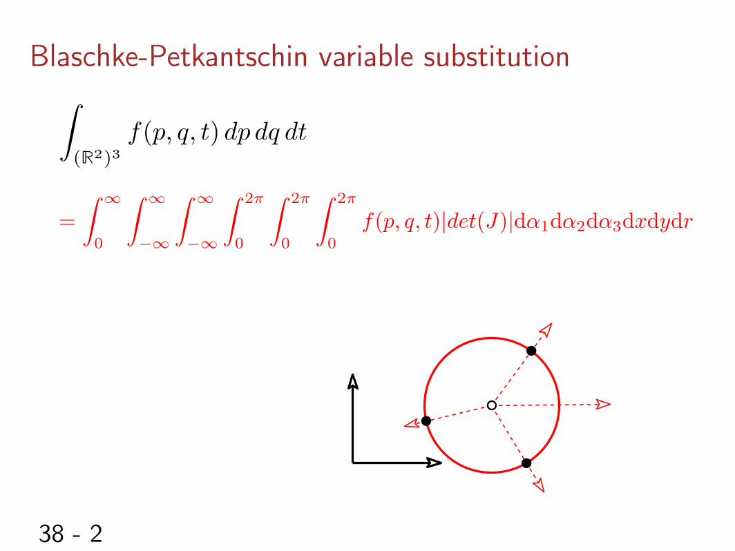
Blaschke-Petkantschin variable substitutionZ

(R2)

3

f(p, q, t) dp dq dt

=

Z 1

0

Z 1

�1

Z 1

�1

Z2⇡

0

Z2⇡

0

Z2⇡

0

f(p, q, t)|det(J)|d↵1

d↵2

d↵3

dxdydr

38 - 3

Blaschke-Petkantschin variable substitutionZ

(R2)

3

f(p, q, t) dp dq dt

=

Z 1

0

Z 1

�1

Z 1

�1

Z2⇡

0

Z2⇡

0

Z2⇡

0

f(p, q, t)|det(J)|d↵1

d↵2

d↵3

dxdydr

=

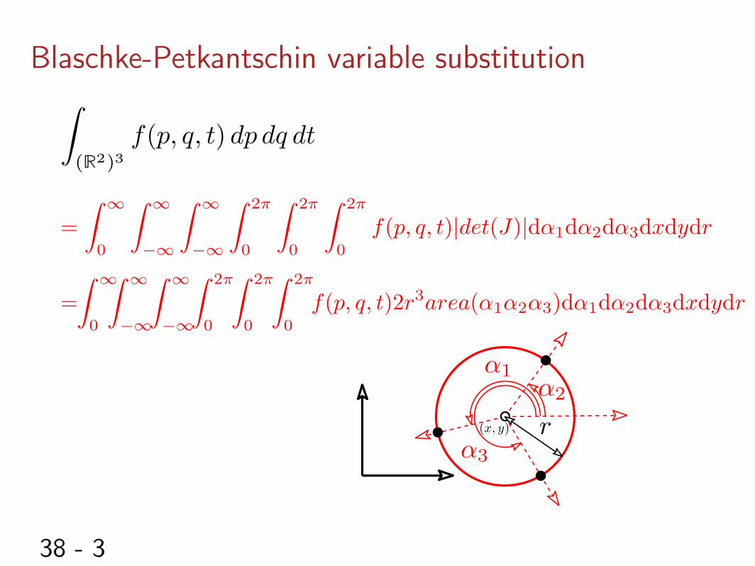
Z 1

0

Z 1

�1

Z 1

�1

Z2⇡

0

Z2⇡

0

Z2⇡

0

f(p, q, t)2r3area(↵1

↵2

↵3

)d↵1

d↵2

d↵3

dxdydr

(x, y) r

↵1

↵2

↵3

39 - 1

Expected number of triangles in conflict with originX a Poisson point process of density n

39 - 2

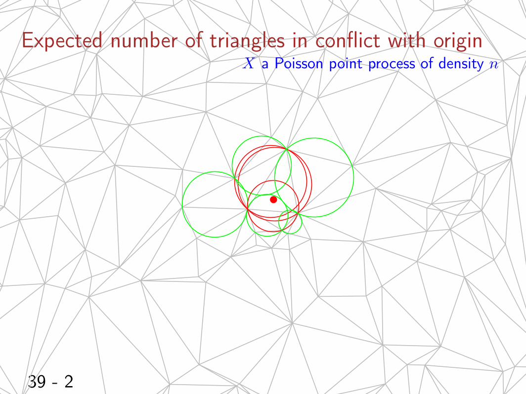
Expected number of triangles in conflict with originX a Poisson point process of density n

39 - 3

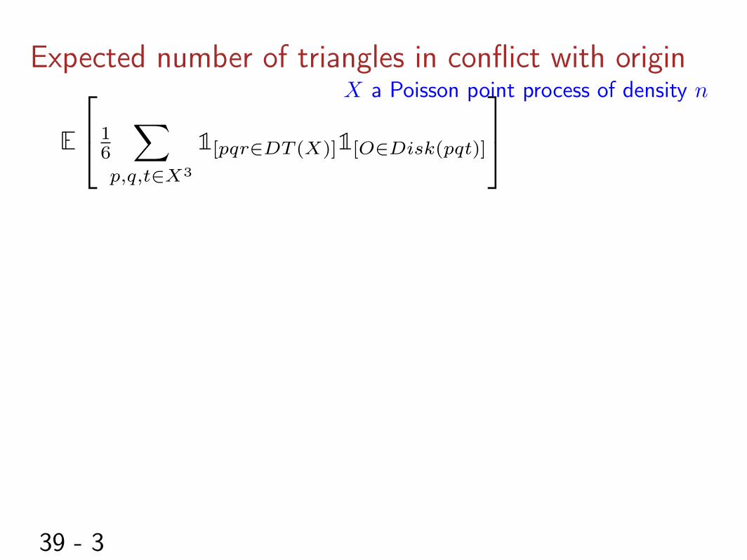
Expected number of triangles in conflict with origin

E

2

4 1

6

X

p,q,t2X3

1[pqr2DT (X)]

1[O2Disk(pqt)]

3

5

X a Poisson point process of density n

39 - 4

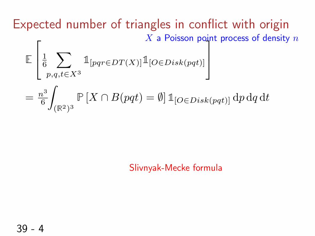
Expected number of triangles in conflict with origin

E

2

4 1

6

X

p,q,t2X3

1[pqr2DT (X)]

1[O2Disk(pqt)]

3

5

=

n3

6

Z

(R2)

3

P [X \B(pqt) = ;] 1[O2Disk(pqt)] dp dq dt

X a Poisson point process of density n

Slivnyak-Mecke formula

39 - 5

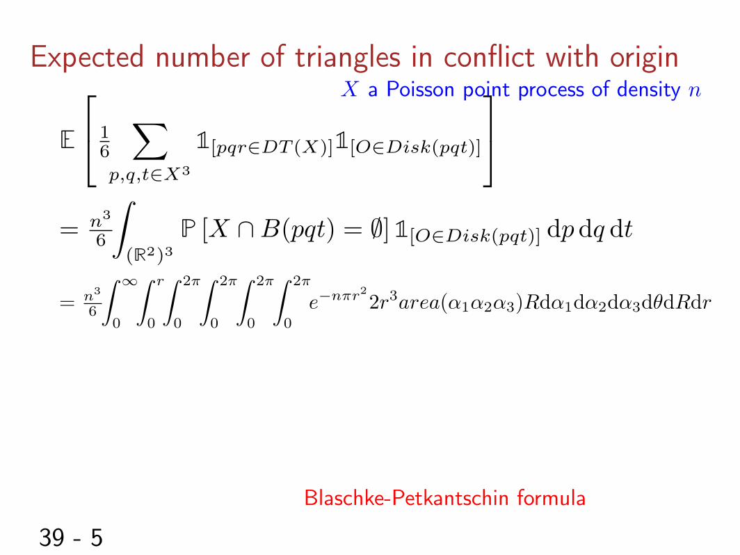
Expected number of triangles in conflict with origin

E

2

4 1

6

X

p,q,t2X3

1[pqr2DT (X)]

1[O2Disk(pqt)]

3

5

=

n3

6

Z

(R2)

3

P [X \B(pqt) = ;] 1[O2Disk(pqt)] dp dq dt

=

n3

6

Z 1

0

Z r

0

Z2⇡

0

Z2⇡

0

Z2⇡

0

Z2⇡

0

e�n⇡r22r3area(↵

1

↵2

↵3

)Rd↵1

d↵2

d↵3

d✓dRdr

X a Poisson point process of density n

Blaschke-Petkantschin formula

39 - 6

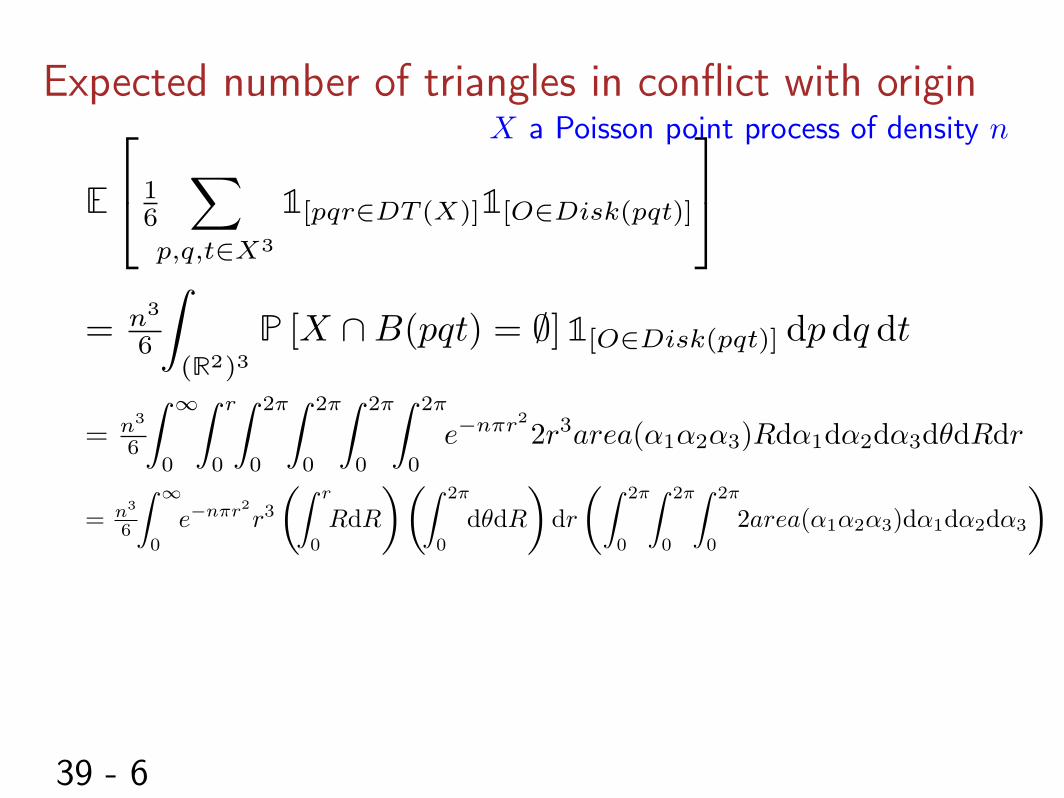
Expected number of triangles in conflict with origin

E

2

4 1

6

X

p,q,t2X3

1[pqr2DT (X)]

1[O2Disk(pqt)]

3

5

=

n3

6

Z

(R2)

3

P [X \B(pqt) = ;] 1[O2Disk(pqt)] dp dq dt

=

n3

6

Z 1

0

Z r

0

Z2⇡

0

Z2⇡

0

Z2⇡

0

Z2⇡

0

e�n⇡r22r3area(↵

1

↵2

↵3

)Rd↵1

d↵2

d↵3

d✓dRdr

=

n3

6

Z 1

0

e�n⇡r2r3ÇZ r

0

RdR

åÇZ2⇡

0

d✓dR

ådr

ÇZ2⇡

0

Z2⇡

0

Z2⇡

0

2area(↵1

↵2

↵3

)d↵1

d↵2

d↵3

å

X a Poisson point process of density n

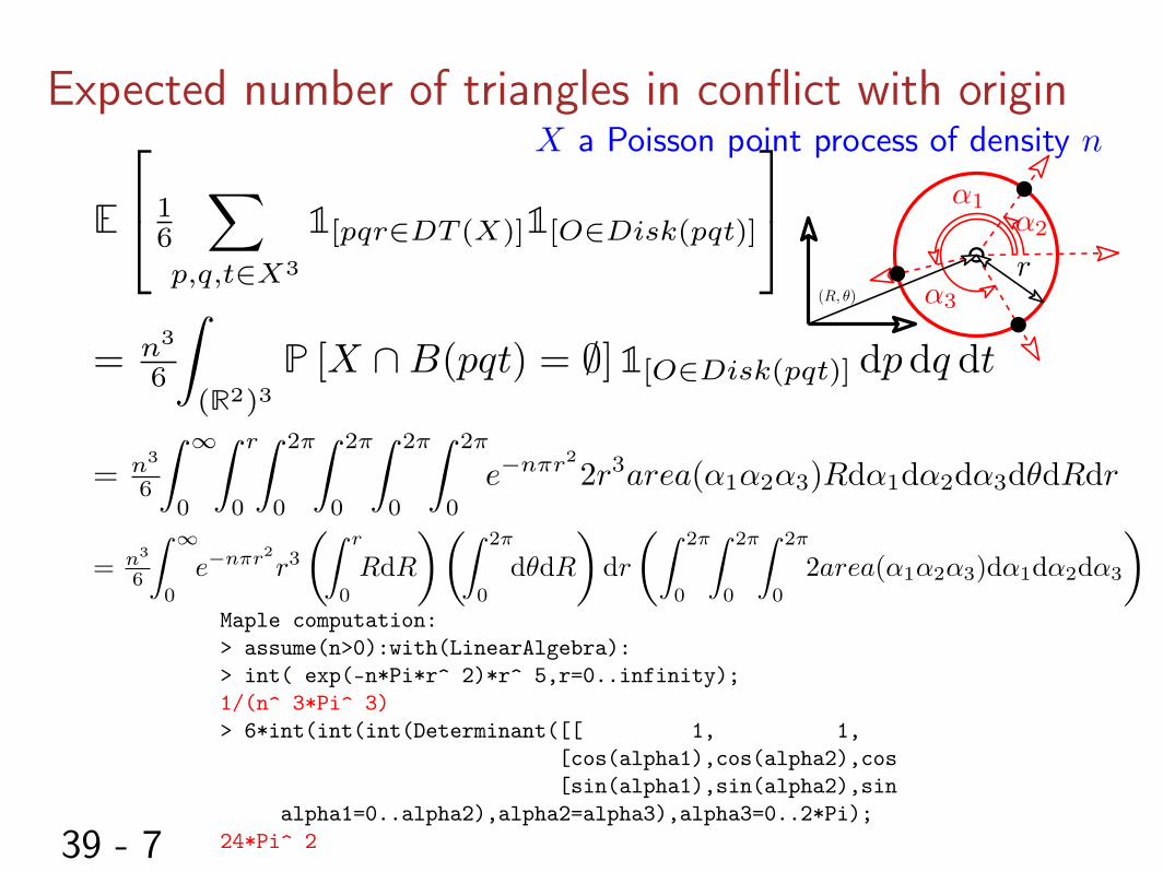
39 - 7

Expected number of triangles in conflict with origin

E

2

4 1

6

X

p,q,t2X3

1[pqr2DT (X)]

1[O2Disk(pqt)]

3

5

=

n3

6

Z

(R2)

3

P [X \B(pqt) = ;] 1[O2Disk(pqt)] dp dq dt

=

n3

6

Z 1

0

Z r

0

Z2⇡

0

Z2⇡

0

Z2⇡

0

Z2⇡

0

e�n⇡r22r3area(↵

1

↵2

↵3

)Rd↵1

d↵2

d↵3

d✓dRdr

=

n3

6

Z 1

0

e�n⇡r2r3ÇZ r

0

RdR

åÇZ2⇡

0

d✓dR

ådr

ÇZ2⇡

0

Z2⇡

0

Z2⇡

0

2area(↵1

↵2

↵3

)d↵1

d↵2

d↵3

å

X a Poisson point process of density n

Maple computation:

> assume(n>0):with(LinearAlgebra):

> int( exp(-n*Pi*r^ 2)*r^ 5,r=0..infinity);

1/(n^ 3*Pi^ 3)

> 6*int(int(int(Determinant([[ 1, 1, 1],

[cos(alpha1),cos(alpha2),cos(alpha3)],

[sin(alpha1),sin(alpha2),sin(alpha3)]]),

alpha1=0..alpha2),alpha2=alpha3),alpha3=0..2*Pi);

24*Pi^ 2

(R, ✓)

r

↵1

↵2

↵3

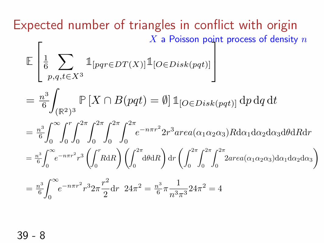
39 - 8

Expected number of triangles in conflict with origin

E

2

4 1

6

X

p,q,t2X3

1[pqr2DT (X)]

1[O2Disk(pqt)]

3

5

=

n3

6

Z

(R2)

3

P [X \B(pqt) = ;] 1[O2Disk(pqt)] dp dq dt

=

n3

6

Z 1

0

Z r

0

Z2⇡

0

Z2⇡

0

Z2⇡

0

Z2⇡

0

e�n⇡r22r3area(↵

1

↵2

↵3

)Rd↵1

d↵2

d↵3

d✓dRdr

=

n3

6

Z 1

0

e�n⇡r2r3ÇZ r

0

RdR

åÇZ2⇡

0

d✓dR

ådr

ÇZ2⇡

0

Z2⇡

0

Z2⇡

0

2area(↵1

↵2

↵3

)d↵1

d↵2

d↵3

å

=

n3

6

Z 1

0

e�n⇡r2r32⇡r2

2

dr 24⇡2

=

n3

6

⇡1

n3⇡3

24⇡2

= 4

X a Poisson point process of density n

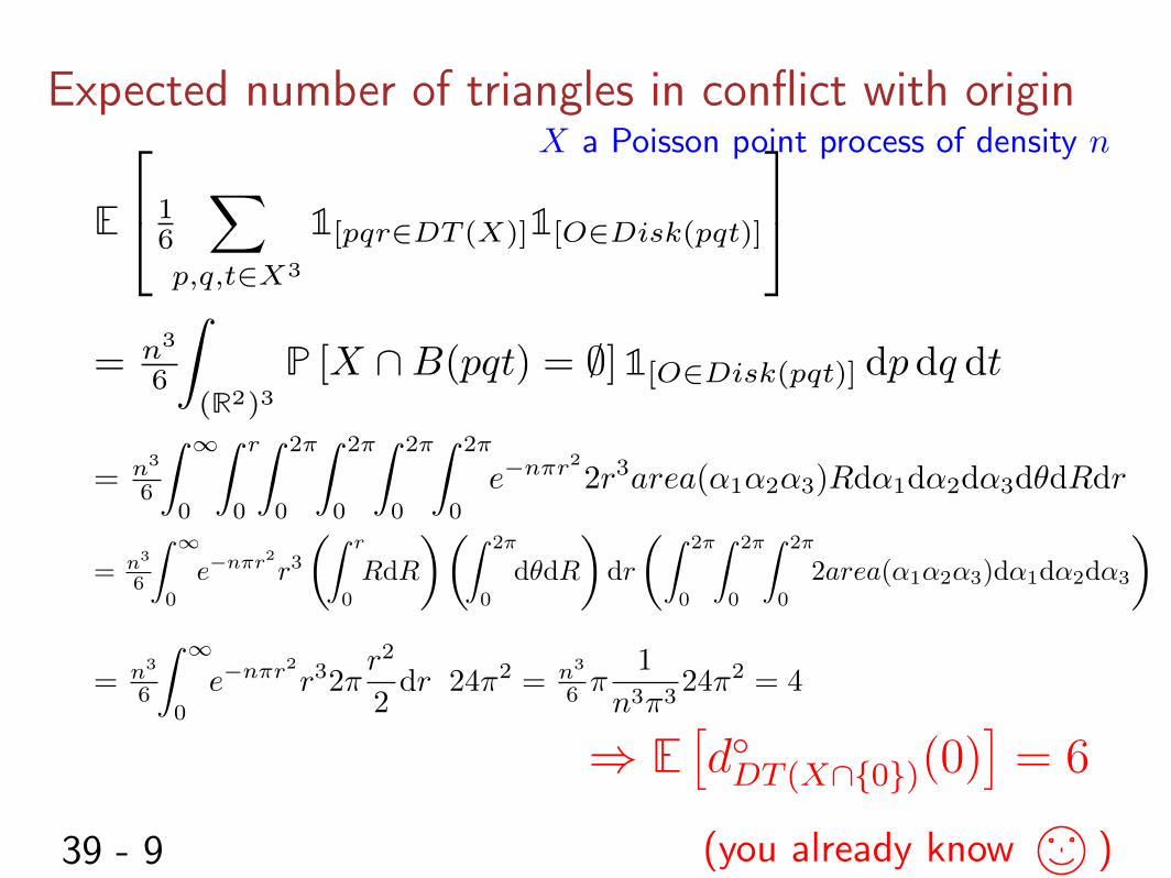
39 - 9

Expected number of triangles in conflict with origin

E

2

4 1

6

X

p,q,t2X3

1[pqr2DT (X)]

1[O2Disk(pqt)]

3

5

=

n3

6

Z

(R2)

3

P [X \B(pqt) = ;] 1[O2Disk(pqt)] dp dq dt

=

n3

6

Z 1

0

Z r

0

Z2⇡

0

Z2⇡

0

Z2⇡

0

Z2⇡

0

e�n⇡r22r3area(↵

1

↵2

↵3

)Rd↵1

d↵2

d↵3

d✓dRdr

=

n3

6

Z 1

0

e�n⇡r2r3ÇZ r

0

RdR

åÇZ2⇡

0

d✓dR

ådr

ÇZ2⇡

0

Z2⇡

0

Z2⇡

0

2area(↵1

↵2

↵3

)d↵1

d↵2

d↵3

å

=

n3

6

Z 1

0

e�n⇡r2r32⇡r2

2

dr 24⇡2

=

n3

6

⇡1

n3⇡3

24⇡2

= 4

) Eîd�DT (X\{0})(0)

ó= 6

(you already know )

X a Poisson point process of density n

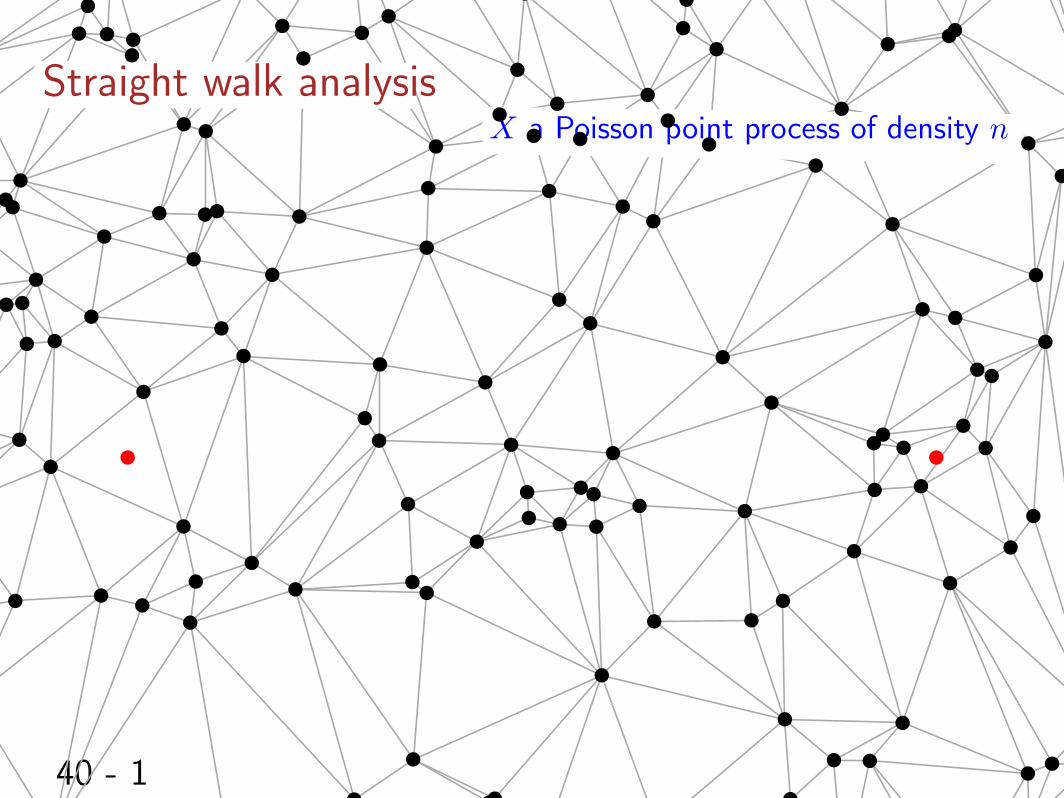
40 - 1

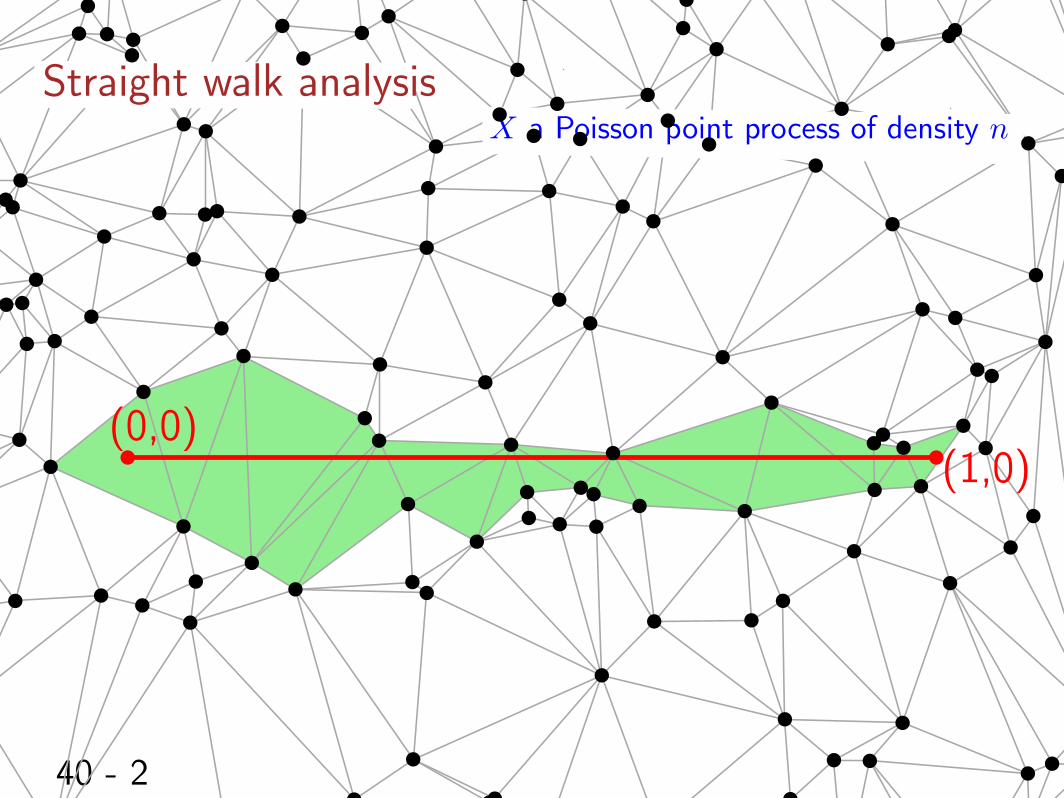
Straight walk analysisX a Poisson point process of density n

40 - 2

Straight walk analysisX a Poisson point process of density n

(0,0)(1,0)

40 - 3

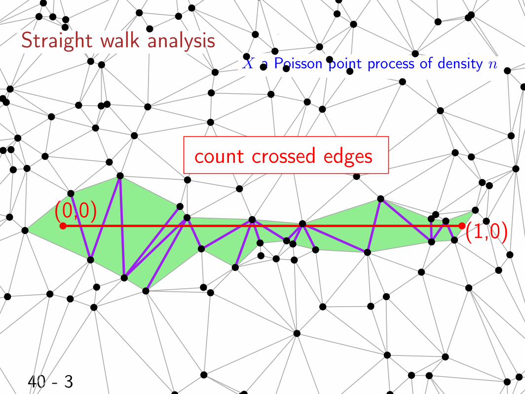
Straight walk analysisX a Poisson point process of density n

(0,0)(1,0)

count crossed edges

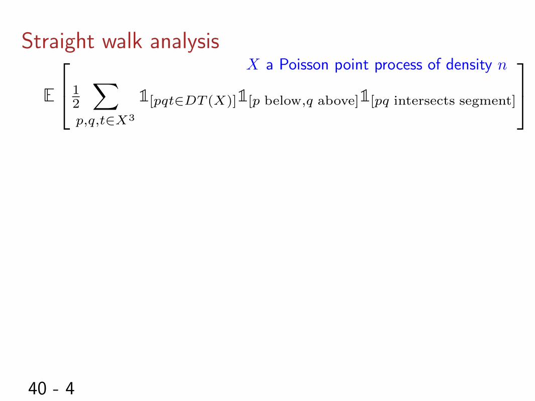
40 - 4

Straight walk analysis

E

2

4 1

2

X

p,q,t2X3

1[pqt2DT (X)]

1[p below,q above]

1[pq intersects segment]

3

5X a Poisson point process of density n

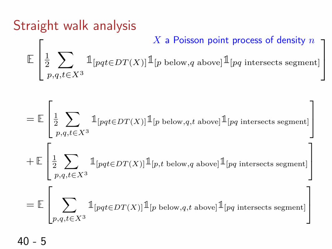
40 - 5

Straight walk analysis

E

2

4 1

2

X

p,q,t2X3

1[pqt2DT (X)]

1[p below,q above]

1[pq intersects segment]

3

5X a Poisson point process of density n

= E

2

4 1

2

X

p,q,t2X3

1[pqt2DT (X)]

1[p below,q,t above]

1[pq intersects segment]

3

5

+E

2

4 1

2

X

p,q,t2X3

1[pqt2DT (X)]

1[p,t below,q above]

1[pq intersects segment]

3

5

= E

2

4X

p,q,t2X3

1[pqt2DT (X)]

1[p below,q,t above]

1[pq intersects segment]

3

5

40 - 6

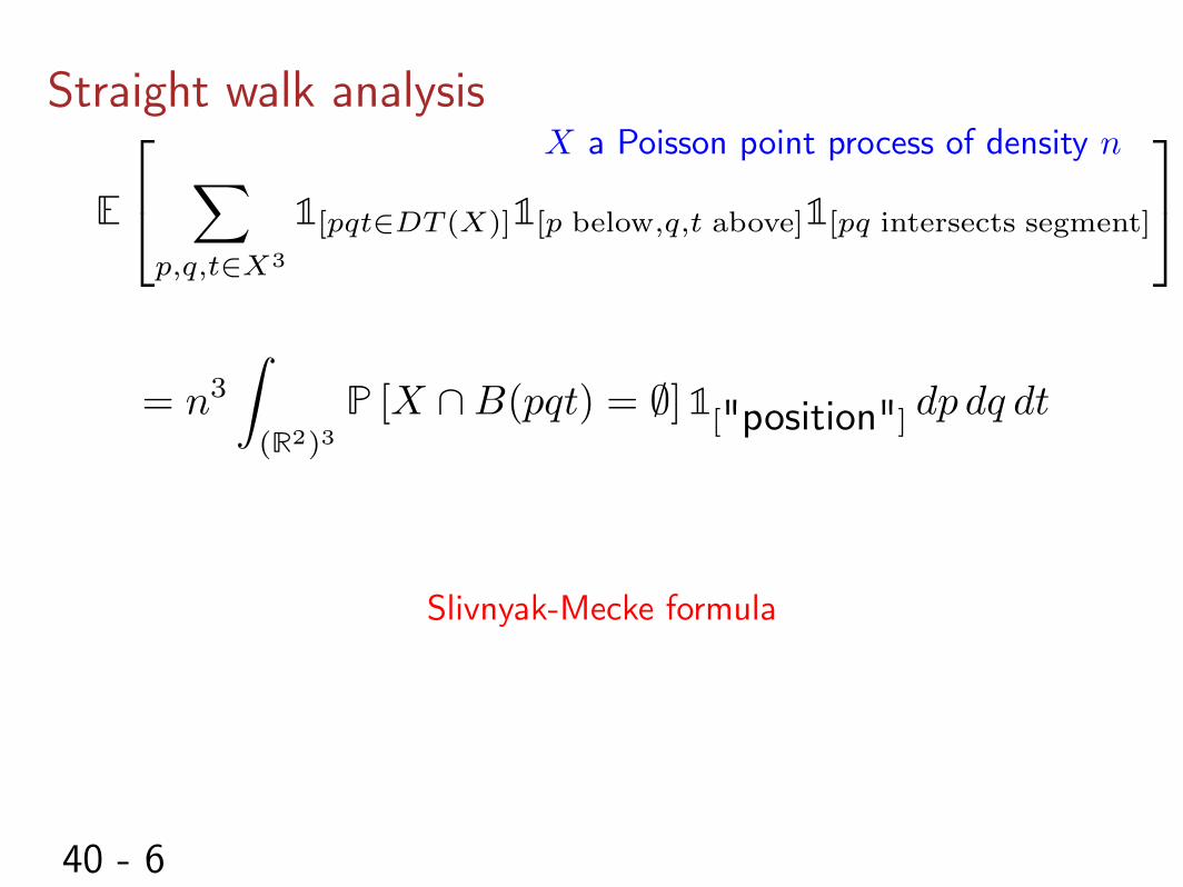
Straight walk analysis

Slivnyak-Mecke formula

= n3

Z

(R2)

3

P [X \B(pqt) = ;] 1["position"] dp dq dt

X a Poisson point process of density n

E

2

4X

p,q,t2X3

1[pqt2DT (X)]

1[p below,q,t above]

1[pq intersects segment]

3

5

40 - 7

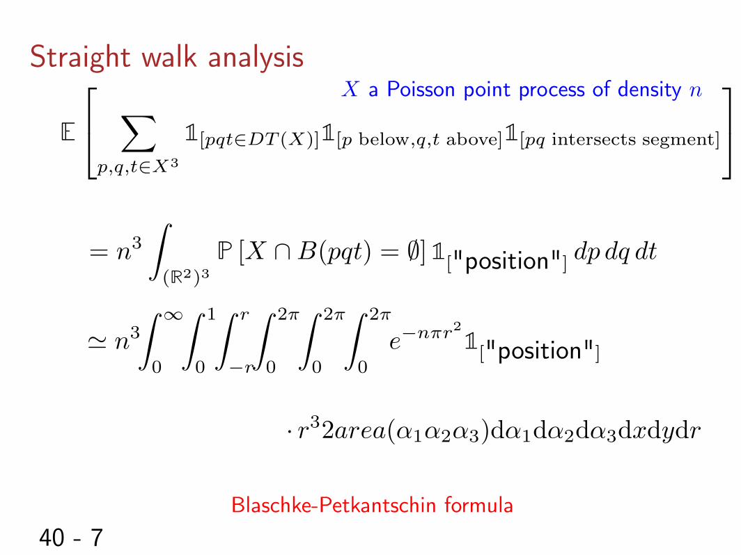
Straight walk analysis

= n3

Z

(R2)

3

P [X \B(pqt) = ;] 1["position"] dp dq dt

Blaschke-Petkantschin formula

· r32area(↵1

↵2

↵3

)d↵1

d↵2

d↵3

dxdydr

' n3

Z 1

0

Z1

0

Z r

�r

Z2⇡

0

Z2⇡

0

Z2⇡

0

e�n⇡r21["position"]

X a Poisson point process of density n

E

2

4X

p,q,t2X3

1[pqt2DT (X)]

1[p below,q,t above]

1[pq intersects segment]

3

5

40 - 8

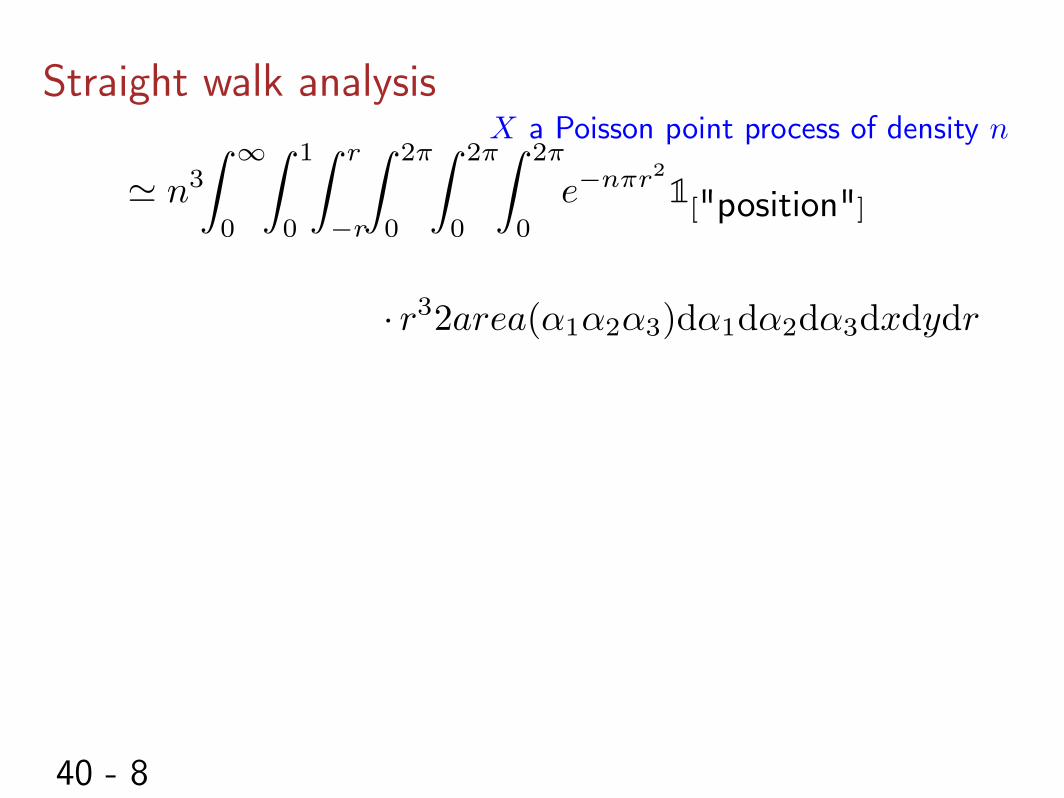
Straight walk analysisX a Poisson point process of density n

· r32area(↵1

↵2

↵3

)d↵1

d↵2

d↵3

dxdydr

' n3

Z 1

0

Z1

0

Z r

�r

Z2⇡

0

Z2⇡

0

Z2⇡

0

e�n⇡r21["position"]

40 - 9

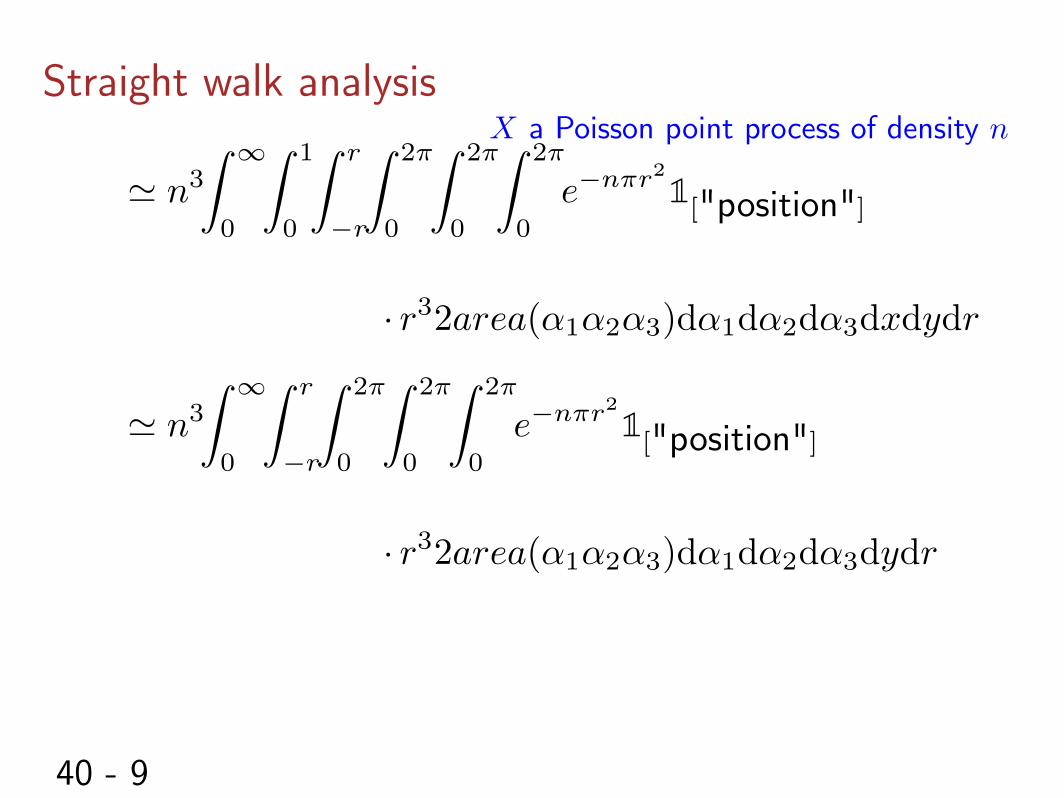
Straight walk analysisX a Poisson point process of density n

· r32area(↵1

↵2

↵3

)d↵1

d↵2

d↵3

dxdydr

' n3

Z 1

0

Z1

0

Z r

�r

Z2⇡

0

Z2⇡

0

Z2⇡

0

e�n⇡r21["position"]

· r32area(↵1

↵2

↵3

)d↵1

d↵2

d↵3

dydr

' n3

Z 1

0

Z r

�r

Z2⇡

0

Z2⇡

0

Z2⇡

0

e�n⇡r21["position"]

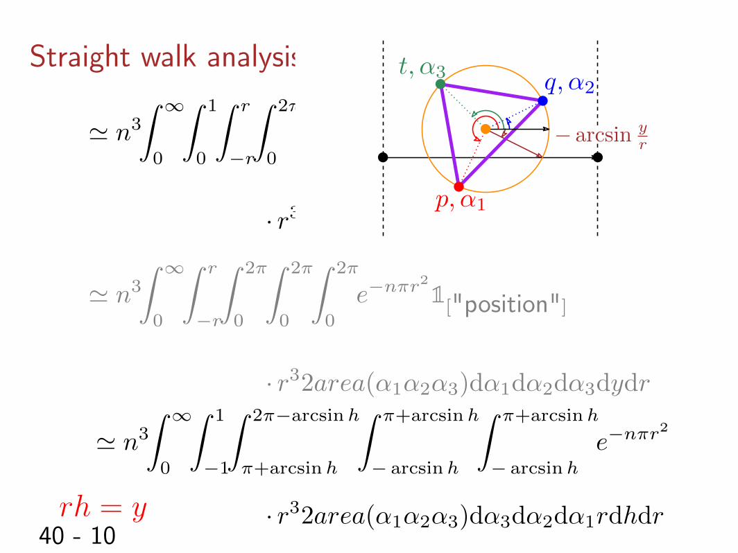
40 - 10

Straight walk analysisX a Poisson point process of density n

· r32area(↵1

↵2

↵3

)d↵1

d↵2

d↵3

dxdydr

' n3

Z 1

0

Z1

0

Z r

�r

Z2⇡

0

Z2⇡

0

Z2⇡

0

e�n⇡r21["position"]

· r32area(↵1

↵2

↵3

)d↵1

d↵2

d↵3

dydr

' n3

Z 1

0

Z r

�r

Z2⇡

0

Z2⇡

0

Z2⇡

0

e�n⇡r21["position"]

· r32area(↵1

↵2

↵3

)d↵3

d↵2

d↵1

rdhdr

' n3

Z 1

0

Z1

�1

Z2⇡�arcsinh

⇡+arcsinh

Z ⇡+arcsinh

� arcsinh

Z ⇡+arcsinh

� arcsinh

e�n⇡r2

rh = y

q,↵2

t,↵3

p,↵1

� arcsin

yr

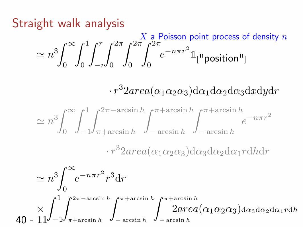
40 - 11

Straight walk analysisX a Poisson point process of density n

· r32area(↵1

↵2

↵3

)d↵1

d↵2

d↵3

dxdydr

' n3

Z 1

0

Z1

0

Z r

�r

Z2⇡

0

Z2⇡

0

Z2⇡

0

e�n⇡r21["position"]

· r32area(↵1

↵2

↵3

)d↵3

d↵2

d↵1

rdhdr

' n3

Z 1

0

Z1

�1

Z2⇡�arcsinh

⇡+arcsinh

Z ⇡+arcsinh

� arcsinh

Z ⇡+arcsinh

� arcsinh

e�n⇡r2

' n3

Z 1

0

e�n⇡r2r3dr

⇥Z

1

�1

Z 2⇡�arcsinh

⇡+arcsinh

Z ⇡+arcsinh

� arcsinh

Z ⇡+arcsinh

� arcsinh

2area(↵1

↵2

↵3

)d↵3d↵2d↵1rdh

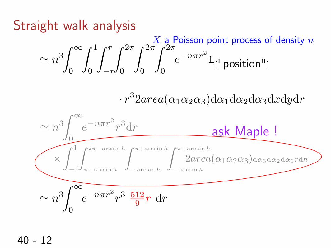
40 - 12

' n3

Z 1

0

e�n⇡r2r3dr

⇥Z

1

�1

Z 2⇡�arcsinh

⇡+arcsinh

Z ⇡+arcsinh

� arcsinh

Z ⇡+arcsinh

� arcsinh

2area(↵1

↵2

↵3

)d↵3d↵2d↵1rdh

Straight walk analysis

512

9

r

X a Poisson point process of density n

· r32area(↵1

↵2

↵3

)d↵1

d↵2

d↵3

dxdydr

' n3

Z 1

0

Z1

0

Z r

�r

Z2⇡

0

Z2⇡

0

Z2⇡

0

e�n⇡r21["position"]

' n3

Z 1

0

e�n⇡r2r3 dr

ask Maple !

40 - 13

' n3

Z 1

0

e�n⇡r2r3dr

⇥Z

1

�1

Z 2⇡�arcsinh

⇡+arcsinh

Z ⇡+arcsinh

� arcsinh

Z ⇡+arcsinh

� arcsinh

2area(↵1

↵2

↵3

)d↵3d↵2d↵1rdh

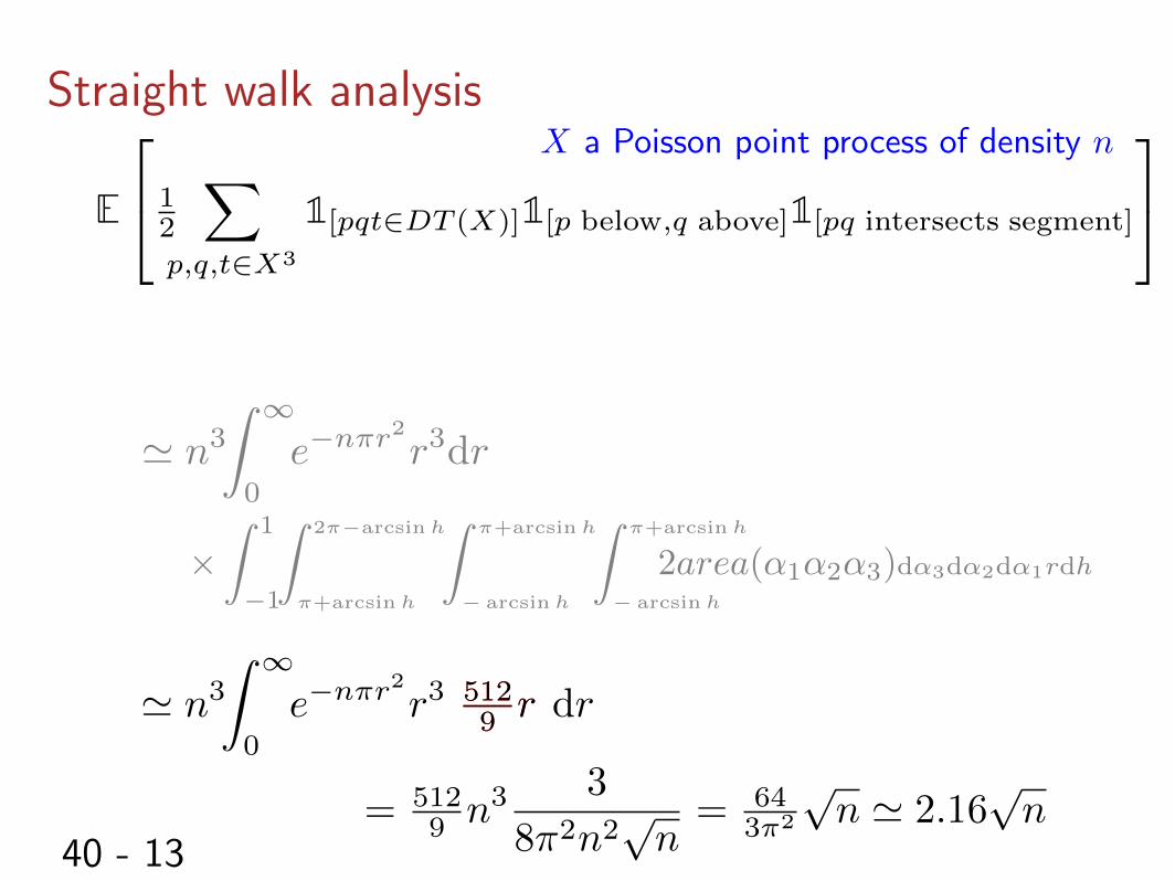
Straight walk analysis

E

2

4 1

2

X

p,q,t2X3

1[pqt2DT (X)]

1[p below,q above]

1[pq intersects segment]

3

5

512

9

r

X a Poisson point process of density n

' n3

Z 1

0

e�n⇡r2r3 dr

=

512

9

n3

3

8⇡2n2

pn=

64

3⇡2

pn ' 2.16

pn

512

9

r

41

Sample of other probabilistic results

42 - 1

Expected degree

E [(d

�(p)] = 62D

42 - 2

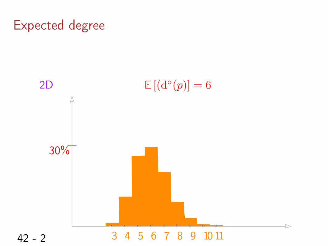
Expected degree

E [(d

�(p)] = 62D

30%

3 4 5 6 7 8 9 10 11

42 - 3

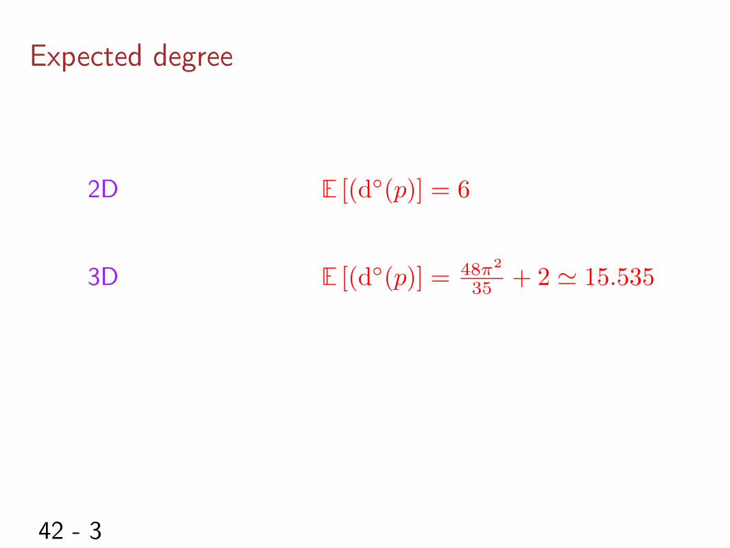
Expected degree

E [(d

�(p)] = 62D

E [(d

�(p)] = 48⇡2

35

+ 2 ' 15.5353D

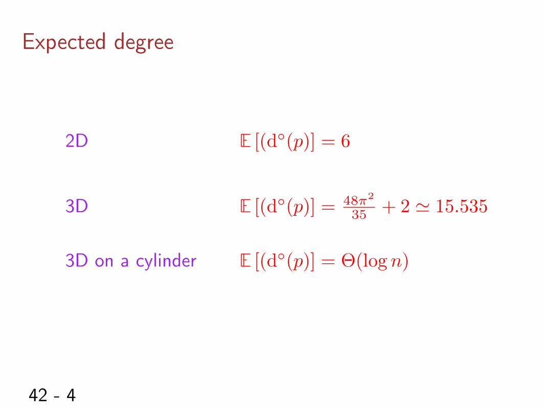
42 - 4

Expected degree

E [(d

�(p)] = 62D

E [(d

�(p)] = 48⇡2

35

+ 2 ' 15.5353D

3D on a cylinder E [(d

�(p)] = ⇥(log n)

42 - 5

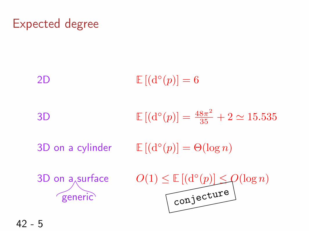
Expected degree

E [(d

�(p)] = 62D

E [(d

�(p)] = 48⇡2

35

+ 2 ' 15.5353D

3D on a cylinder E [(d

�(p)] = ⇥(log n)

3D on a surface O(1) E [(d

�(p)] O(log n)

c

o

n

j

e

c

t

u

r

egeneric

43 - 1

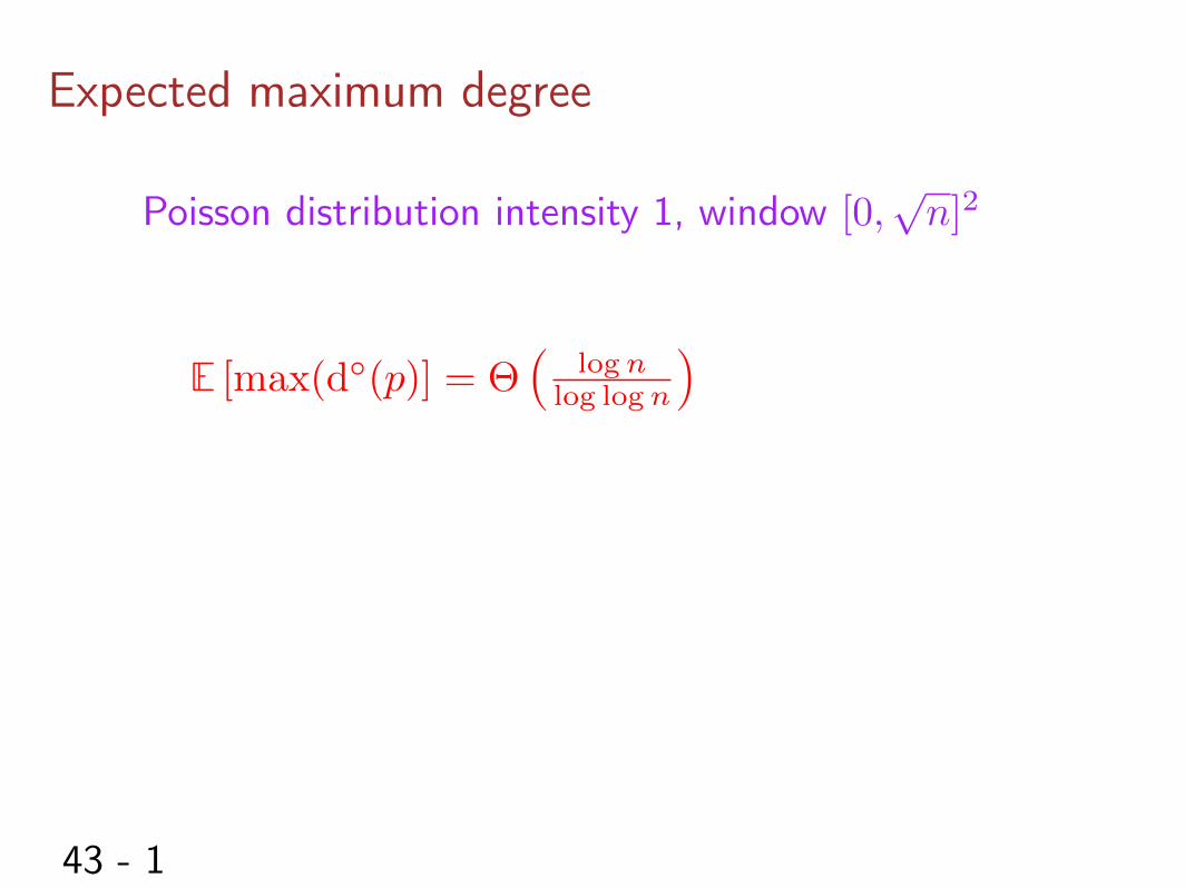
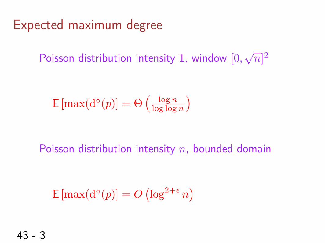
Expected maximum degree

Poisson distribution intensity 1, window [0,pn]2

E [max(d

�(p)] = ⇥

Älogn

log logn

ä

43 - 2

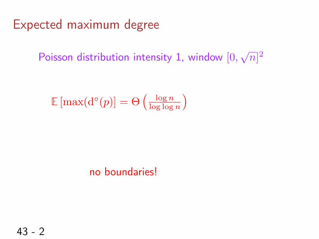
Expected maximum degree

Poisson distribution intensity 1, window [0,pn]2

E [max(d

�(p)] = ⇥

Älogn

log logn

ä

no boundaries!

43 - 3

Expected maximum degree

Poisson distribution intensity 1, window [0,pn]2

E [max(d

�(p)] = ⇥

Älogn

log logn

ä

Poisson distribution intensity n, bounded domain

E [max(d

�(p)] = O

�log

2+✏ n�

44 - 1

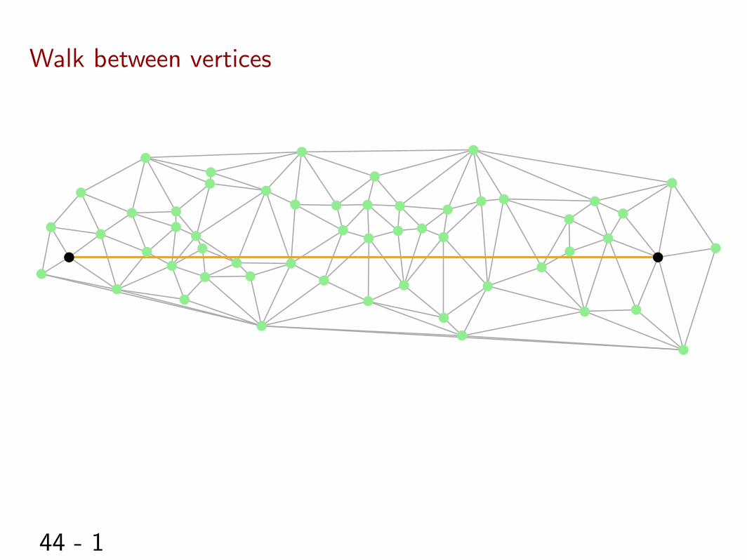
Walk between vertices

44 - 2

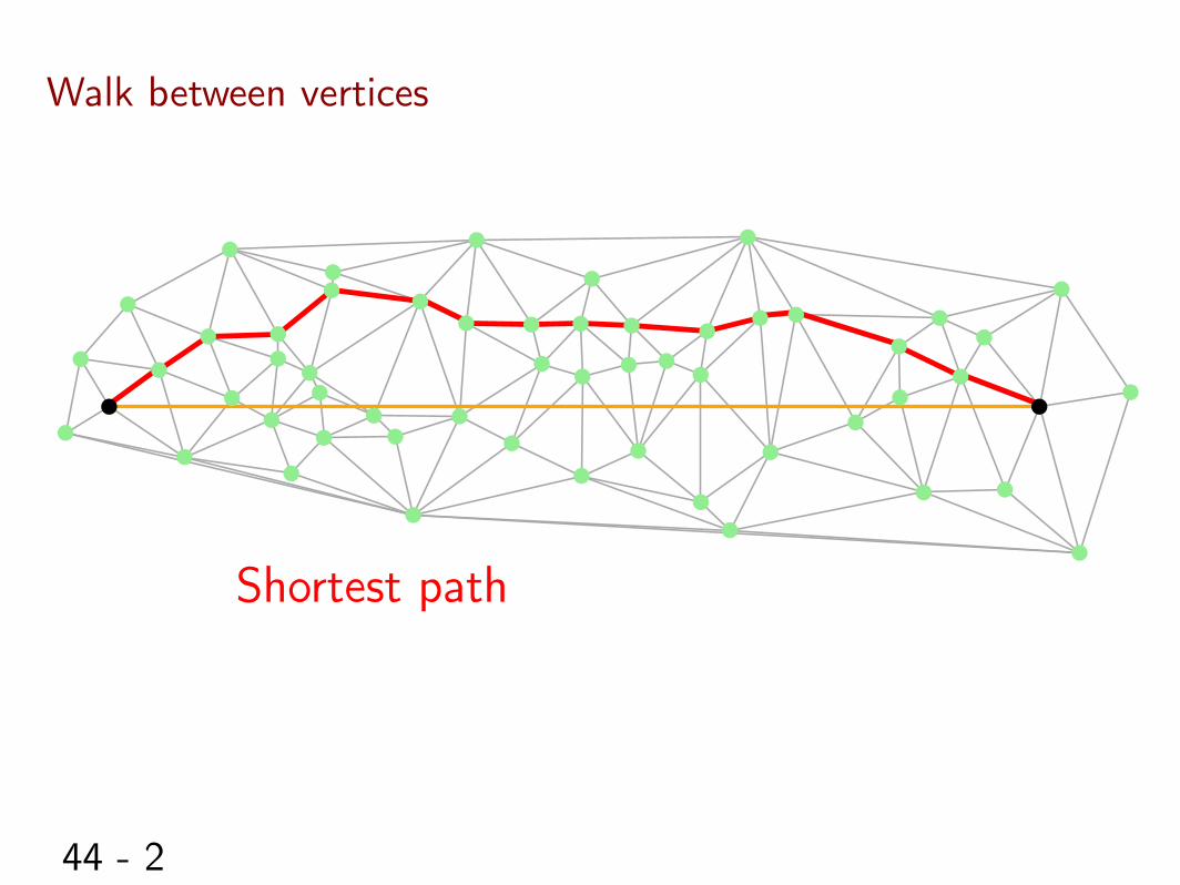
Walk between vertices

Shortest path

44 - 3

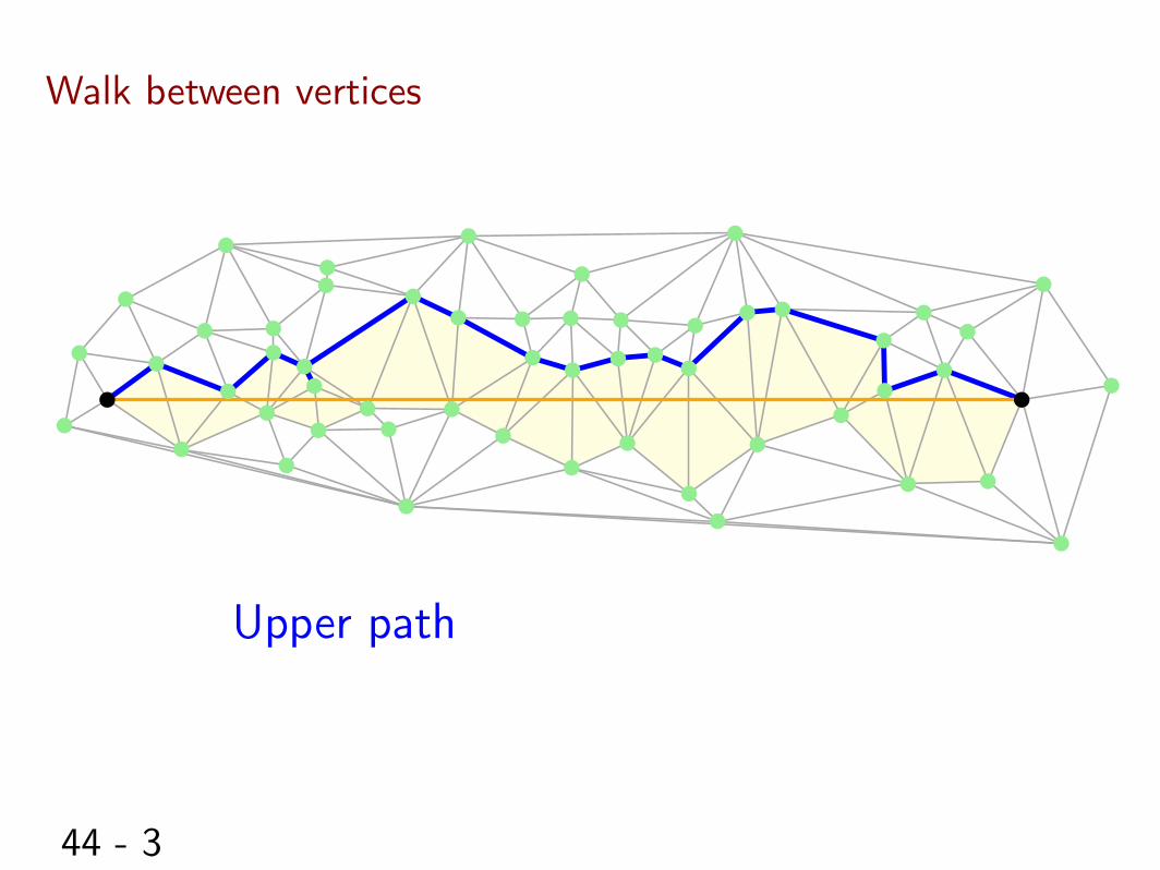
Walk between vertices

Upper path

44 - 4

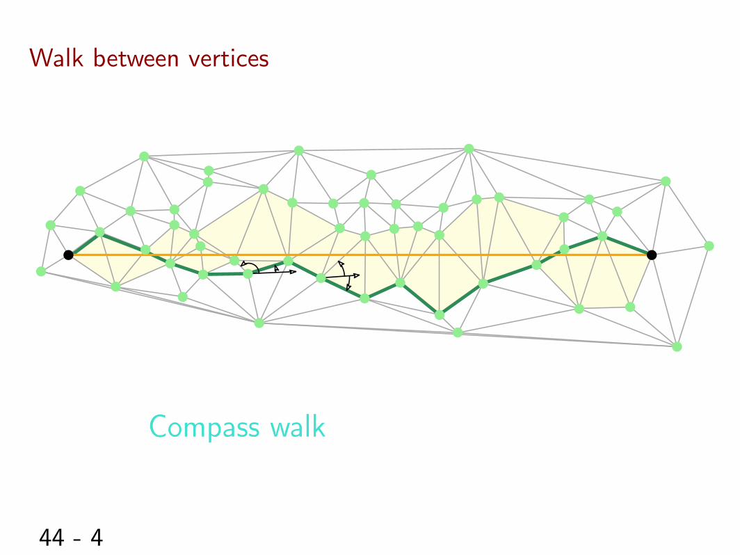
Walk between vertices

Compass walk

44 - 5

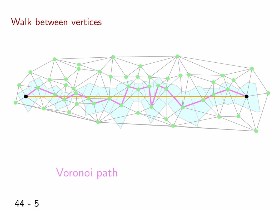
Walk between vertices

Voronoi path

44 - 6

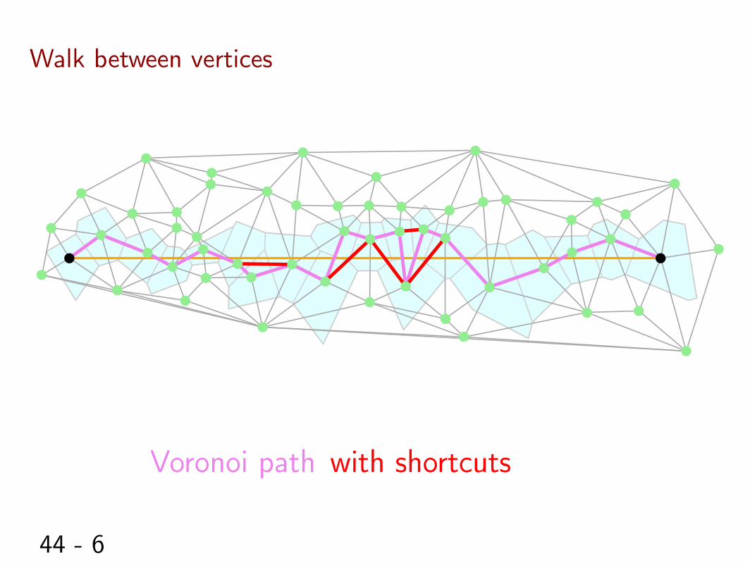
Walk between vertices

Voronoi path with shortcuts

44 - 7

Walk between vertices

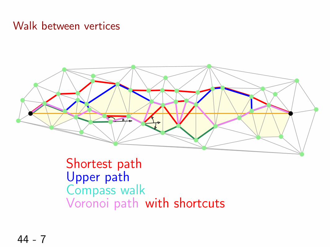
Shortest pathUpper path

Voronoi path with shortcutsCompass walk

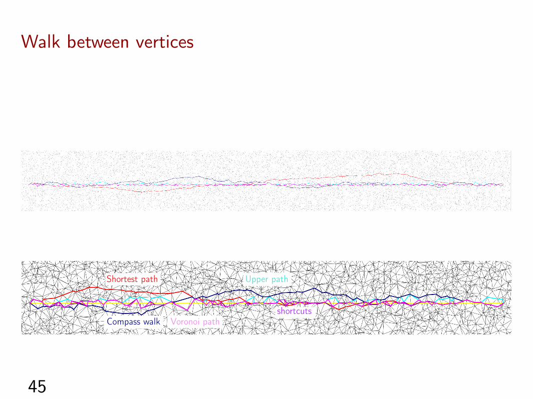
45

Upper path

Voronoi path

shortcuts

Shortest path

Compass walk

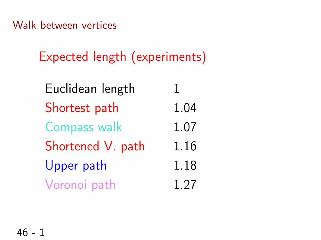
Walk between vertices

46 - 1

Shortest path

Upper pathVoronoi path

Shortened V. pathCompass walk

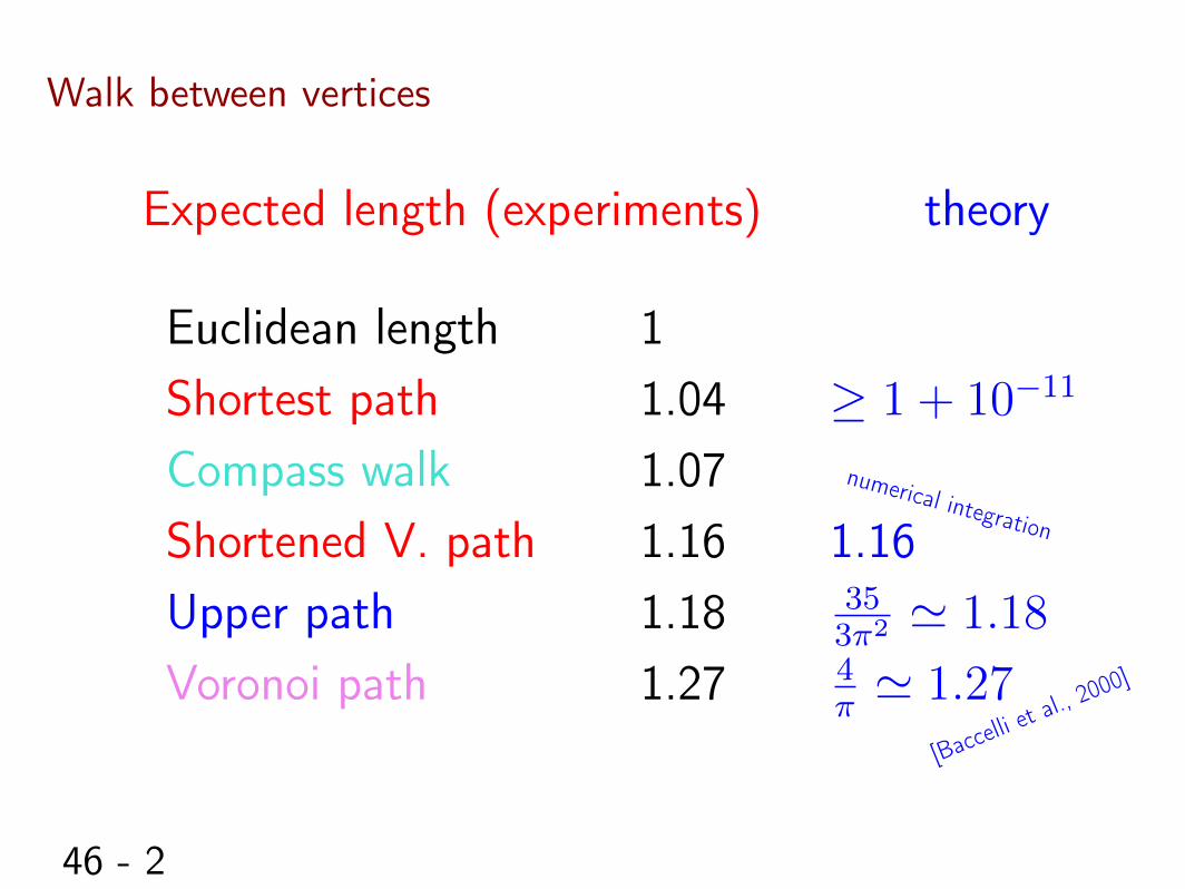
Expected length (experiments)

Euclidean length 11.041.071.161.181.27

Walk between vertices

46 - 2

Shortest path

Upper pathVoronoi path

Shortened V. pathCompass walk

Expected length (experiments)

Euclidean length 11.041.071.161.181.27

theory

� 1 + 10

�11

1.16n

u

m

e

r

i

c

a

l

i

n

t

e

g

r

a

t

i

o

n

35

3⇡2 ' 1.184

⇡ ' 1.27

[

B

a

c

c

e

l

l

i

e

t

a

l

.

,

2

0

0

0

]

Walk between vertices

47 - 1

Smoothed analysis of convex hull

47 - 2

Smoothed analysis of convex hull

K unit ball of Rd

47 - 3

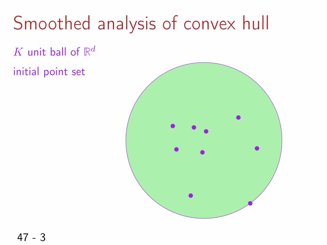
Smoothed analysis of convex hull

K unit ball of Rd

initial point set

47 - 4

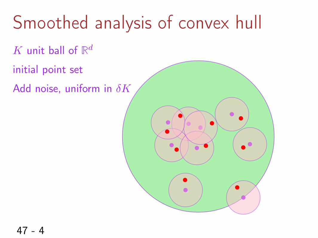
Smoothed analysis of convex hull

K unit ball of Rd

initial point set

Add noise, uniform in �K

47 - 5

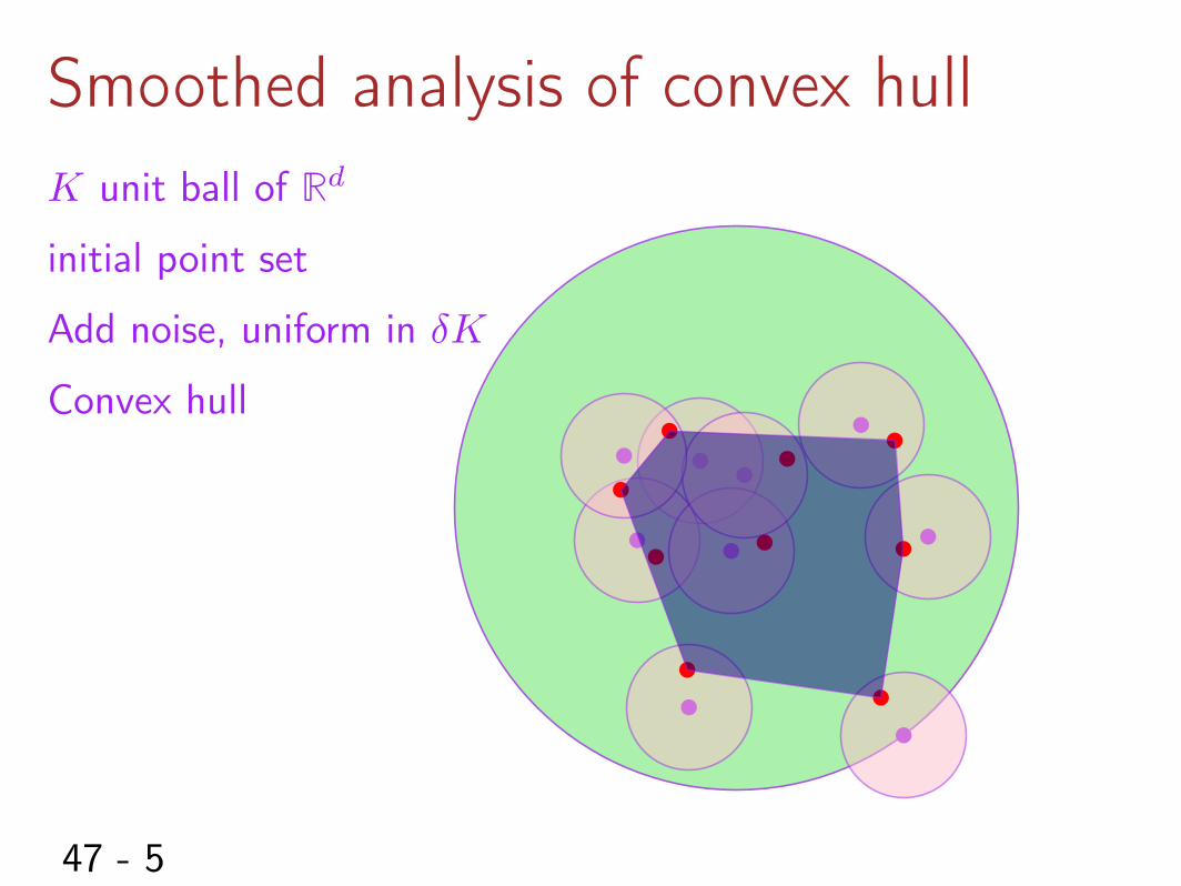
Smoothed analysis of convex hull

K unit ball of Rd

initial point set

Add noise, uniform in �K

Convex hull

47 - 6

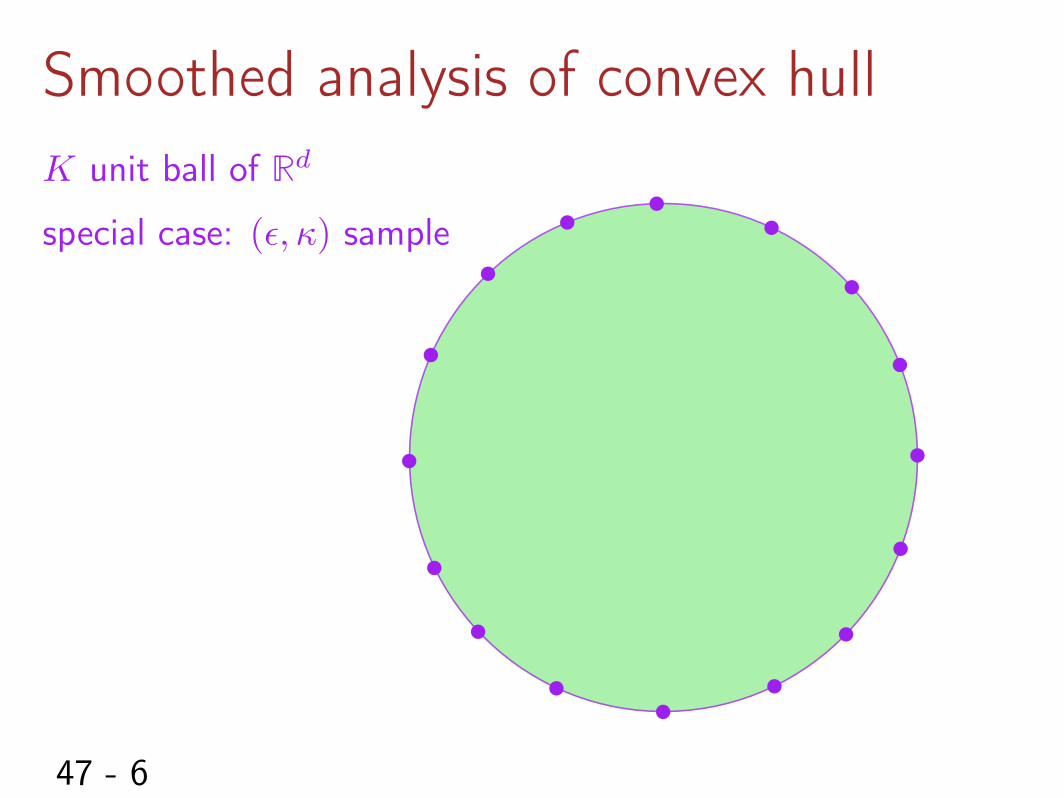
Smoothed analysis of convex hull

K unit ball of Rd

special case: (✏,) sample

47 - 7

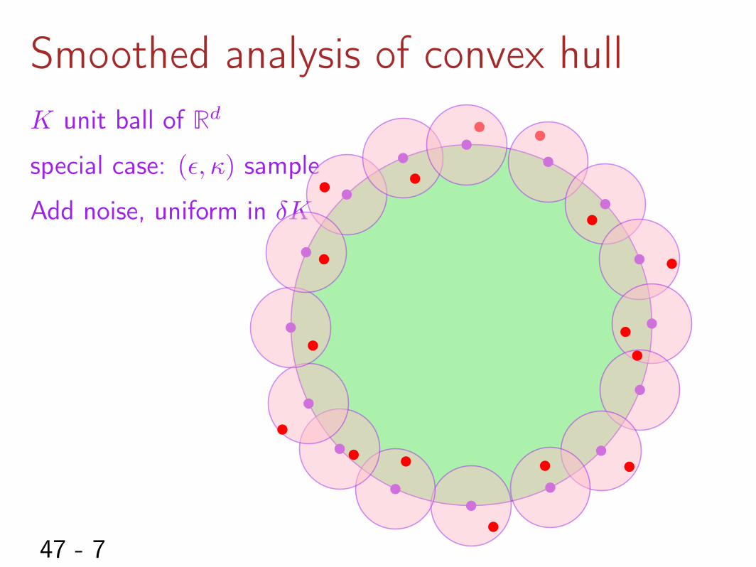
Smoothed analysis of convex hull

K unit ball of Rd

special case: (✏,) sample

Add noise, uniform in �K

47 - 8

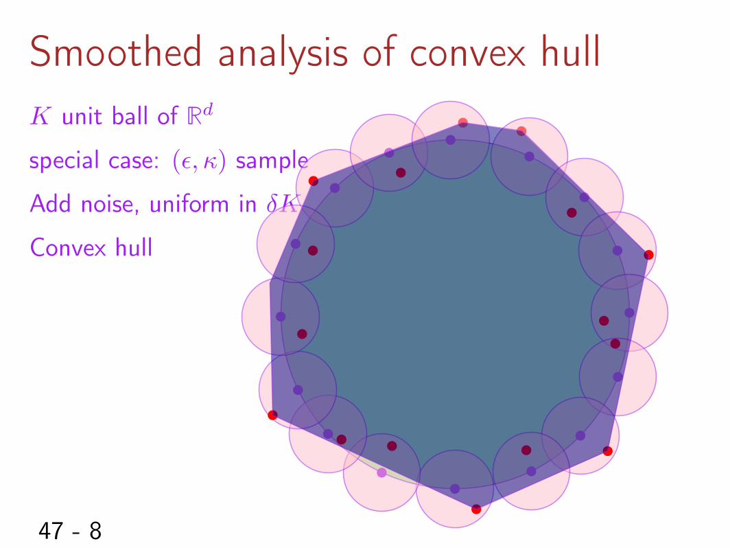
Smoothed analysis of convex hull

K unit ball of Rd

special case: (✏,) sample

Add noise, uniform in �K

Convex hull

47 - 9

Smoothed analysis of convex hull

1

2

0

1

3

1

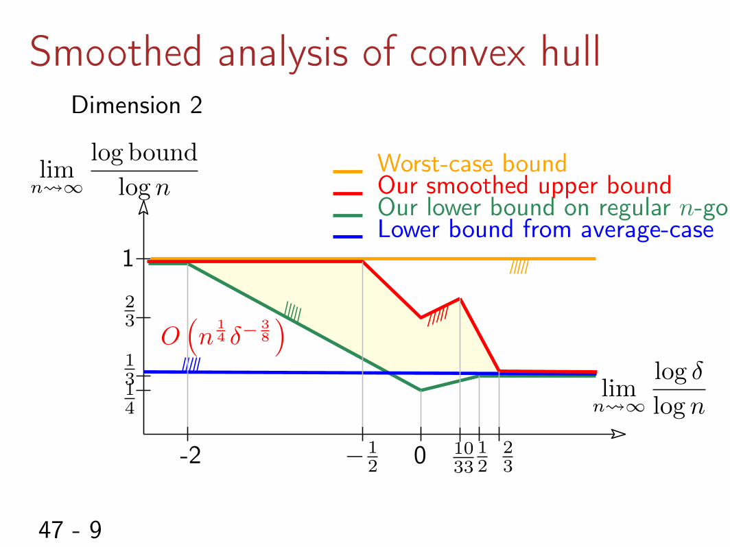
Worst-case boundOur smoothed upper boundOur lower bound on regular n-gonLower bound from average-case

lim

n 1

log �

log n

lim

n 1

log bound

log n

1

4

2

3

-2

Dimension 2

2

3

10

33

� 1

2

OÄn

14 ��

38

ä

47 - 10

Smoothed analysis of convex hull

Open problems

Tighter analysis for CH

Delaunay size in 3D

Delaunay walk in 2D

48The end