point processing & filtering - university of …cs194-26/fa16/lectures/...point processing &...

Point Processing & Filtering

CS194: Image Manipulation & Computational Photography Alexei Efros, UC Berkeley, Fall 2016

Image Formation

f(x,y) = reflectance(x,y) * illumination(x,y) Reflectance in [0,1], illumination in [0,inf]

Problem: Dynamic Range

1500

1

25,000

400,000

2,000,000,000

The real world is High dynamic range

Long Exposure

10-6 106

10-6 106

Real world

Picture

0 to 255

High dynamic range

Short Exposure

10-6 106

10-6 106

Real world

Picture

0 to 255

High dynamic range

scene radiance

(W/sr/m )

∫ sensor irradiance

sensor exposure

Lens Shutter

2

∆t

analog voltages

digital values

pixel values

CCD ADC Remapping

Image Acquisition Pipeline

Simple Point Processing: Enhancement

Power-law transformations

Basic Point Processing

Negative

Contrast Stretching

Image Histograms

Cumulative Histograms

s = T(r)

Histogram Equalization

Color Transfer [Reinhard, et al, 2001]

Erik Reinhard, Michael Ashikhmin, Bruce Gooch, Peter Shirley, Color Transfer between Images. IEEE Computer Graphics and Applications, 21(5), pp. 34–41. September 2001.

http://www.cs.bris.ac.uk/Publications/pub_master.jsp?id=2000476

http://www.cs.bris.ac.uk/Publications/pub_master.jsp?id=2000476

Limitations of Point Processing Q: What happens if I reshuffle all pixels within

the image? A: It’s histogram won’t change. No point

processing will be affected…

What is an image? We can think of an image as a function, f, from R2 to

R: • f( x, y ) gives the intensity at position ( x, y ) • Realistically, we expect the image only to be defined over a

rectangle, with a finite range: – f: [a,b]x[c,d] [0,1]

A color image is just three functions pasted together.

We can write this as a “vector-valued” function:

( , )( , ) ( , )

( , )

r x yf x y g x y

b x y

=

Images as functions

Sampling and Reconstruction

© 2006 Steve Marschner • 20

Sampled representations

• How to store and compute with continuous functions?

• Common scheme for representation: samples – write down the function’s values at many points

[FvD

FH fi

g.14

.14b

/ W

olbe

rg]


Reconstruction

• Making samples back into a continuous function – for output (need realizable method) – for analysis or processing (need mathematical method) – amounts to “guessing” what the function did in between

[FvD

FH fi

g.14

.14b

/ W

olbe

rg]

1D Example: Audio

low high frequencies


Sampling in digital audio

• Recording: sound to analog to samples to disc

• Playback: disc to samples to analog to sound again – how can we be sure we are filling in the gaps correctly?


Sampling and Reconstruction

• Simple example: a sign wave


Undersampling

• What if we “missed” things between the samples?

• Simple example: undersampling a sine wave – unsurprising result: information is lost


Undersampling


• Simple example: undersampling a sine wave – unsurprising result: information is lost – surprising result: indistinguishable from lower frequency


Undersampling


• Simple example: undersampling a sine wave – unsurprising result: information is lost – surprising result: indistinguishable from lower frequency – also, was always indistinguishable from higher frequencies – aliasing: signals “traveling in disguise” as other frequencies

Aliasing in video

Slide by Steve Seitz

Aliasing in images

What’s happening? Input signal:

x = 0:.05:5; imagesc(sin((2.^x).*x))

Plot as image:

Alias! Not enough samples

Antialiasing What can we do about aliasing? Sample more often

• Join the Mega-Pixel craze of the photo industry • But this can’t go on forever

Make the signal less “wiggly”

• Get rid of some high frequencies • Will loose information • But it’s better than aliasing


Preventing aliasing

• Introduce lowpass filters: – remove high frequencies leaving only safe, low frequencies – choose lowest frequency in reconstruction (disambiguate)


Linear filtering: a key idea

• Transformations on signals; e.g.: – bass/treble controls on stereo – blurring/sharpening operations in image editing – smoothing/noise reduction in tracking

• Key properties – linearity: filter(f + g) = filter(f) + filter(g) – shift invariance: behavior invariant to shifting the input

• delaying an audio signal • sliding an image around

• Can be modeled mathematically by convolution


Moving Average

• basic idea: define a new function by averaging over a sliding window

• a simple example to start off: smoothing


Moving Average

• Can add weights to our moving average

• Weights […, 0, 1, 1, 1, 1, 1, 0, …] / 5

Cross-correlation

This is called a cross-correlation operation:

Let be the image, be the kernel (of size 2k+1 x 2k+1), and be the output image

• Can think of as a “dot product” between local neighborhood and kernel for each pixel

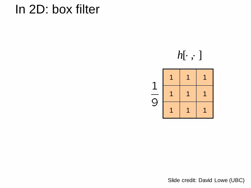
1 1 1

1 1 1

1 1 1

Slide credit: David Lowe (UBC)

],[ ⋅⋅h

In 2D: box filter

0 0 0 0 0 0 0 0 0 0

0 0 0 0 0 0 0 0 0 0

0 0 0 90 90 90 90 90 0 0

0 0 0 90 90 90 90 90 0 0

0 0 0 90 90 90 90 90 0 0

0 0 0 90 0 90 90 90 0 0

0 0 0 90 90 90 90 90 0 0

0 0 0 0 0 0 0 0 0 0

0 0 90 0 0 0 0 0 0 0

0 0 0 0 0 0 0 0 0 0

0

0 0 0 0 0 0 0 0 0 0

0 0 0 0 0 0 0 0 0 0

0 0 0 90 90 90 90 90 0 0

0 0 0 90 90 90 90 90 0 0

0 0 0 90 90 90 90 90 0 0

0 0 0 90 0 90 90 90 0 0

0 0 0 90 90 90 90 90 0 0

0 0 0 0 0 0 0 0 0 0

0 0 90 0 0 0 0 0 0 0

0 0 0 0 0 0 0 0 0 0

Credit: S. Seitz

],[],[],[,

lnkmflkhnmglk

++= ∑

[.,.]g[.,.]f

Image filtering 1 1 1

1 1 1

1 1 1

],[ ⋅⋅h

0 0 0 0 0 0 0 0 0 0

0 0 0 0 0 0 0 0 0 0

0 0 0 90 90 90 90 90 0 0

0 0 0 90 90 90 90 90 0 0

0 0 0 90 90 90 90 90 0 0

0 0 0 90 0 90 90 90 0 0

0 0 0 90 90 90 90 90 0 0

0 0 0 0 0 0 0 0 0 0

0 0 90 0 0 0 0 0 0 0

0 0 0 0 0 0 0 0 0 0

0 10

0 0 0 0 0 0 0 0 0 0

0 0 0 0 0 0 0 0 0 0

0 0 0 90 90 90 90 90 0 0

0 0 0 90 90 90 90 90 0 0

0 0 0 90 90 90 90 90 0 0

0 0 0 90 0 90 90 90 0 0

0 0 0 90 90 90 90 90 0 0

0 0 0 0 0 0 0 0 0 0

0 0 90 0 0 0 0 0 0 0

0 0 0 0 0 0 0 0 0 0

[.,.]g[.,.]f


1 1 1

1 1 1

],[ ⋅⋅h

Credit: S. Seitz

],[],[],[,

lnkmflkhnmglk

++= ∑

0 0 0 0 0 0 0 0 0 0

0 0 0 0 0 0 0 0 0 0

0 0 0 90 90 90 90 90 0 0

0 0 0 90 90 90 90 90 0 0

0 0 0 90 90 90 90 90 0 0

0 0 0 90 0 90 90 90 0 0

0 0 0 90 90 90 90 90 0 0

0 0 0 0 0 0 0 0 0 0

0 0 90 0 0 0 0 0 0 0

0 0 0 0 0 0 0 0 0 0

0 10 20

0 0 0 0 0 0 0 0 0 0

0 0 0 0 0 0 0 0 0 0

0 0 0 90 90 90 90 90 0 0

0 0 0 90 90 90 90 90 0 0

0 0 0 90 90 90 90 90 0 0

0 0 0 90 0 90 90 90 0 0

0 0 0 90 90 90 90 90 0 0

0 0 0 0 0 0 0 0 0 0

0 0 90 0 0 0 0 0 0 0

0 0 0 0 0 0 0 0 0 0

[.,.]g[.,.]f


1 1 1

1 1 1

],[ ⋅⋅h

Credit: S. Seitz

0 0 0 0 0 0 0 0 0 0

0 0 0 0 0 0 0 0 0 0

0 0 0 90 90 90 90 90 0 0

0 0 0 90 90 90 90 90 0 0

0 0 0 90 90 90 90 90 0 0

0 0 0 90 0 90 90 90 0 0

0 0 0 90 90 90 90 90 0 0

0 0 0 0 0 0 0 0 0 0

0 0 90 0 0 0 0 0 0 0

0 0 0 0 0 0 0 0 0 0

0 10 20 30

0 0 0 0 0 0 0 0 0 0

0 0 0 0 0 0 0 0 0 0

0 0 0 90 90 90 90 90 0 0

0 0 0 90 90 90 90 90 0 0

0 0 0 90 90 90 90 90 0 0

0 0 0 90 0 90 90 90 0 0

0 0 0 90 90 90 90 90 0 0

0 0 0 0 0 0 0 0 0 0

0 0 90 0 0 0 0 0 0 0

0 0 0 0 0 0 0 0 0 0

[.,.]g[.,.]f


1 1 1

1 1 1

],[ ⋅⋅h

Credit: S. Seitz

0 10 20 30 30

0 0 0 0 0 0 0 0 0 0

0 0 0 0 0 0 0 0 0 0

0 0 0 90 90 90 90 90 0 0

0 0 0 90 90 90 90 90 0 0

0 0 0 90 90 90 90 90 0 0

0 0 0 90 0 90 90 90 0 0

0 0 0 90 90 90 90 90 0 0

0 0 0 0 0 0 0 0 0 0

0 0 90 0 0 0 0 0 0 0

0 0 0 0 0 0 0 0 0 0

[.,.]g[.,.]f


1 1 1

1 1 1

],[ ⋅⋅h

Credit: S. Seitz

0 10 20 30 30

0 0 0 0 0 0 0 0 0 0

0 0 0 0 0 0 0 0 0 0

0 0 0 90 90 90 90 90 0 0

0 0 0 90 90 90 90 90 0 0

0 0 0 90 90 90 90 90 0 0

0 0 0 90 0 90 90 90 0 0

0 0 0 90 90 90 90 90 0 0

0 0 0 0 0 0 0 0 0 0

0 0 90 0 0 0 0 0 0 0

0 0 0 0 0 0 0 0 0 0

[.,.]g[.,.]f


1 1 1

1 1 1

],[ ⋅⋅h

Credit: S. Seitz

?

0 10 20 30 30

50

0 0 0 0 0 0 0 0 0 0

0 0 0 0 0 0 0 0 0 0

0 0 0 90 90 90 90 90 0 0

0 0 0 90 90 90 90 90 0 0

0 0 0 90 90 90 90 90 0 0

0 0 0 90 0 90 90 90 0 0

0 0 0 90 90 90 90 90 0 0

0 0 0 0 0 0 0 0 0 0

0 0 90 0 0 0 0 0 0 0

0 0 0 0 0 0 0 0 0 0

[.,.]g[.,.]f


1 1 1

1 1 1

],[ ⋅⋅h

Credit: S. Seitz

?

0 0 0 0 0 0 0 0 0 0

0 0 0 0 0 0 0 0 0 0

0 0 0 90 90 90 90 90 0 0

0 0 0 90 90 90 90 90 0 0

0 0 0 90 90 90 90 90 0 0

0 0 0 90 0 90 90 90 0 0

0 0 0 90 90 90 90 90 0 0

0 0 0 0 0 0 0 0 0 0

0 0 90 0 0 0 0 0 0 0

0 0 0 0 0 0 0 0 0 0

0 10 20 30 30 30 20 10

0 20 40 60 60 60 40 20

0 30 60 90 90 90 60 30

0 30 50 80 80 90 60 30

0 30 50 80 80 90 60 30

0 20 30 50 50 60 40 20

10 20 30 30 30 30 20 10

10 10 10 0 0 0 0 0

[.,.]g[.,.]f

Image filtering 1 1 1 1 1 1 1 1 1 ],[ ⋅⋅h

Credit: S. Seitz

],[],[],[,

lnkmflkhnmglk

++= ∑

What does it do? • Replaces each pixel with

an average of its neighborhood

• Achieve smoothing effect (remove sharp features)

1 1 1

1 1 1

1 1 1

Slide credit: David Lowe (UBC)

],[ ⋅⋅h

Box Filter

Linear filters: examples

Original

1 1 1 1 1 1 1 1 1

Blur (with a mean filter)

Source: D. Lowe

=

Practice with linear filters

0 0 0 0 1 0 0 0 0

Original

?

Source: D. Lowe


0 0 0 0 1 0 0 0 0

Original Filtered (no change)

Source: D. Lowe


0 0 0 0 0 1 0 0 0

Original

?

Source: D. Lowe


0 0 0 1 0 0 0 0 0

Original Shifted left By 1 pixel

Source: D. Lowe

Other filters

-1 0 1

-2 0 2

-1 0 1

Vertical Edge (absolute value)

Sobel

Other filters

-1 -2 -1

0 0 0

1 2 1

Horizontal Edge (absolute value)

Sobel

Q?

Back to the box filter


Moving Average

• Can add weights to our moving average

• Weights […, 0, 1, 1, 1, 1, 1, 0, …] / 5


Weighted Moving Average

• bell curve (gaussian-like) weights […, 1, 4, 6, 4, 1, …]


Moving Average In 2D

What are the weights H?

0 0 0 0 0 0 0 0 0 0 0 0 0 0 0 0 0 0 0 0 0 0 0 90 90 90 90 90 0 0 0 0 0 90 90 90 90 90 0 0 0 0 0 90 90 90 90 90 0 0 0 0 0 90 0 90 90 90 0 0 0 0 0 90 90 90 90 90 0 0 0 0 0 0 0 0 0 0 0 0 0 0 90 0 0 0 0 0 0 0 0 0 0 0 0 0 0 0 0 0


60

Gaussian filtering A Gaussian kernel gives less weight to pixels further from the center of the window

This kernel is an approximation of a Gaussian function:

0 0 0 0 0 0 0 0 0 0

0 0 0 0 0 0 0 0 0 0

0 0 0 90 90 90 90 90 0 0

0 0 0 90 90 90 90 90 0 0

0 0 0 90 90 90 90 90 0 0

0 0 0 90 0 90 90 90 0 0

0 0 0 90 90 90 90 90 0 0

0 0 0 0 0 0 0 0 0 0

0 0 90 0 0 0 0 0 0 0

0 0 0 0 0 0 0 0 0 0

1 2 1

2 4 2

1 2 1


61

Mean vs. Gaussian filtering


62

Weight contributions of neighboring pixels by nearness

0.003 0.013 0.022 0.013 0.003 0.013 0.059 0.097 0.059 0.013 0.022 0.097 0.159 0.097 0.022 0.013 0.059 0.097 0.059 0.013 0.003 0.013 0.022 0.013 0.003

5 x 5, σ = 1

Slide credit: Christopher Rasmussen

Important filter: Gaussian

63

Gaussian Kernel

• Standard deviation σ: determines extent of smoothing

Source: K. Grauman

σ = 2 with 30 x 30 kernel

σ = 5 with 30 x 30 kernel

Gaussian filters

= 30 pixels = 1 pixel = 5 pixels = 10 pixels

65

Choosing kernel width • The Gaussian function has infinite support, but discrete filters

use finite kernels

Source: K. Grauman

66

How big should the filter be?

Values at edges should be near zero

Rule of thumb for Gaussian: set filter half-width to about 3 σ

Practical matters

Side by Derek Hoiem

Cross-correlation vs. Convolution cross-correlation: A convolution operation is a cross-correlation where the filter is

flipped both horizontally and vertically before being applied to the image:

It is written: Convolution is commutative and associative


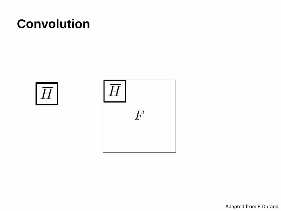
Convolution

Adapted from F. Durand


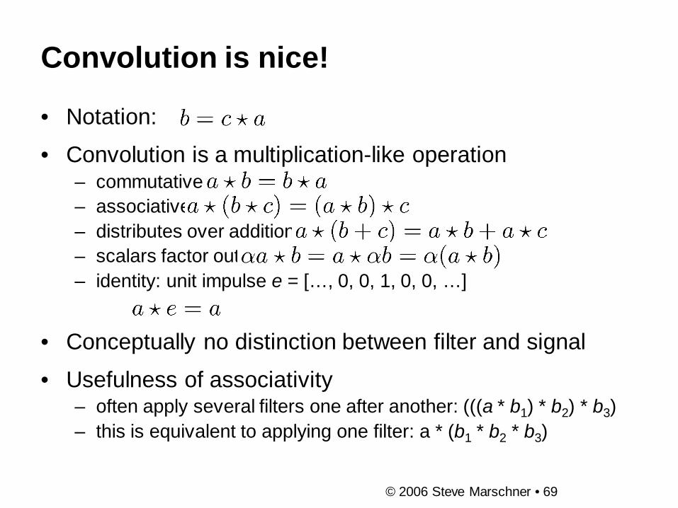
Convolution is nice!

• Notation:

• Convolution is a multiplication-like operation – commutative – associative – distributes over addition – scalars factor out – identity: unit impulse e = […, 0, 0, 1, 0, 0, …]

• Conceptually no distinction between filter and signal

• Usefulness of associativity – often apply several filters one after another: (((a * b1) * b2) * b3) – this is equivalent to applying one filter: a * (b1 * b2 * b3)

Gaussian and convolution • Removes “high-frequency” components from

the image (low-pass filter) • Convolution with self is another Gaussian

– Convolving twice with Gaussian kernel of width = convolving once with kernel of width

Source: K. Grauman

* =

Image half-sizing

This image is too big to fit on the screen. How can we reduce it? How to generate a half- sized version?

Image sub-sampling

Throw away every other row and column to create a 1/2 size image

- called image sub-sampling

1/4

1/8


Image sub-sampling

1/4 (2x zoom) 1/8 (4x zoom)

Aliasing! What do we do?

1/2


Sampling an image

Examples of GOOD sampling

Undersampling

Examples of BAD sampling -> Aliasing

Gaussian (lowpass) pre-filtering

G 1/4

G 1/8

Gaussian 1/2

Solution: filter the image, then subsample • Filter size should double for each ½ size reduction. Why?


Subsampling with Gaussian pre-filtering

G 1/4 G 1/8 Gaussian 1/2


Compare with...

1/4 (2x zoom) 1/8 (4x zoom) 1/2


Gaussian (lowpass) pre-filtering

G 1/4

G 1/8

Gaussian 1/2

Solution: filter the image, then subsample • Filter size should double for each ½ size reduction. Why? • How can we speed this up? Slide by Steve Seitz

Image Pyramids

Known as a Gaussian Pyramid [Burt and Adelson, 1983] • In computer graphics, a mip map [Williams, 1983] • A precursor to wavelet transform


A bar in the big images is a hair on the zebra’s nose; in smaller images, a stripe; in the smallest, the animal’s nose

Figure from David Forsyth

Gaussian pyramid construction

filter mask

Repeat • Filter • Subsample

Until minimum resolution reached • can specify desired number of levels (e.g., 3-level pyramid)

The whole pyramid is only 4/3 the size of the original image! Slide by Steve Seitz

What are they good for? Improve Search

• Search over translations – Classic coarse-to-fine strategy

• Search over scale – Template matching – E.g. find a face at different scales

Taking derivative by convolution

Partial derivatives with convolution

For 2D function f(x,y), the partial derivative is:

For discrete data, we can approximate using finite differences: To implement above as convolution, what would be the associated filter?

εε

ε

),(),(lim),(0

yxfyxfx

yxf −+=

∂∂

→

1),(),1(),( yxfyxf

xyxf −+

≈∂

∂

Source: K. Grauman

Partial derivatives of an image

Which shows changes with respect to x?

-1 1

1 -1 or -1 1

xyxf

∂∂ ),(

yyxf

∂∂ ),(

Finite difference filters Other approximations of derivative filters exist:

Source: K. Grauman

The gradient points in the direction of most rapid increase in intensity

Image gradient

The gradient of an image:

The gradient direction is given by

Source: Steve Seitz

The edge strength is given by the gradient magnitude

• How does this direction relate to the direction of the edge?

Image Gradient

xyxf

∂∂ ),(

yyxf

∂∂ ),(

Effects of noise Consider a single row or column of the image

• Plotting intensity as a function of position gives a signal

Where is the edge? Source: S. Seitz

Solution: smooth first

• To find edges, look for peaks in )( gfdxd

∗

f

g

f * g

)( gfdxd

∗

Source: S. Seitz

Derivative theorem of convolution

This saves us one operation:

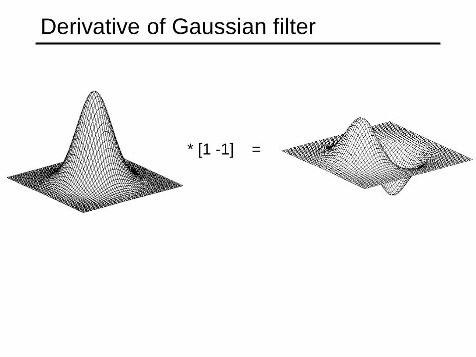
Derivative of Gaussian filter

* [1 -1] =

Derivative of Gaussian filter

Which one finds horizontal/vertical edges?

x-direction y-direction

Example

input image (“Lena”)

Compute Gradients (DoG)

X-Derivative of Gaussian

Y-Derivative of Gaussian

Gradient Magnitude

Get Orientation at Each Pixel Threshold at minimum level Get orientation

theta = atan2(-gy, gx)

MATLAB demo

im = im2double(imread(filemane)); g = fspecial('gaussian',15,2); imagesc(g); surfl(g); gim = conv2(im,g,'same'); imagesc(conv2(im,[-1 1],'same')); imagesc(conv2(gim,[-1 1],'same')); dx = conv2(g,[-1 1],'same'); Surfl(dx); imagesc(conv2(im,dx,'same'));

Practical matters What is the size of the output? MATLAB: filter2(g, f, shape) or conv2(g,f,shape)

• shape = ‘full’: output size is sum of sizes of f and g • shape = ‘same’: output size is same as f • shape = ‘valid’: output size is difference of sizes of f and g

f

g g

g g

f

g g

g g

f

g g

g g

full same valid

Source: S. Lazebnik

Practical matters What about near the edge?

• the filter window falls off the edge of the image • need to extrapolate • methods:

– clip filter (black) – wrap around – copy edge – reflect across edge

Source: S. Marschner

Practical matters

• methods (MATLAB): – clip filter (black): imfilter(f, g, 0) – wrap around: imfilter(f, g, ‘circular’) – copy edge: imfilter(f, g, ‘replicate’) – reflect across edge: imfilter(f, g, ‘symmetric’)

Source: S. Marschner

Q?

Review: Smoothing vs. derivative filters Smoothing filters

• Gaussian: remove “high-frequency” components; “low-pass” filter

• Can the values of a smoothing filter be negative? • What should the values sum to?

– One: constant regions are not affected by the filter

Derivative filters • Derivatives of Gaussian • Can the values of a derivative filter be negative? • What should the values sum to?

– Zero: no response in constant regions • High absolute value at points of high contrast

Template matching Goal: find in image Main challenge: What is a

good similarity or distance measure between two patches? • Correlation • Zero-mean correlation • Sum Square Difference • Normalized Cross Correlation

Side by Derek Hoiem

Matching with filters Goal: find in image Method 0: filter the image with eye patch

Input Filtered Image

],[],[],[,

lnkmflkgnmhlk

++= ∑

What went wrong?

f = image g = filter

Side by Derek Hoiem

Matching with filters Goal: find in image Method 1: filter the image with zero-mean eye

Input Filtered Image (scaled) Thresholded Image

)],[()],[(],[,

lnkmgflkfnmhlk

++−= ∑

True detections

False detections

mean of f

Matching with filters Goal: find in image Method 2: SSD

Input 1- sqrt(SSD) Thresholded Image

2

,

)],[],[(],[ lnkmflkgnmhlk

++−= ∑

True detections

Matching with filters Can SSD be implemented with linear filters?

2

,


++−= ∑

Side by Derek Hoiem

Matching with filters Goal: find in image Method 2: SSD

Input 1- sqrt(SSD)

2

,


++−= ∑

What’s the potential downside of SSD?

Side by Derek Hoiem

Matching with filters Goal: find in image Method 3: Normalized cross-correlation

5.0

,

2,

,

2

,,

)],[()],[(

)],[)(],[(],[

−++−

−++−=

∑ ∑

∑

lknm

lk

nmlk

flnkmfglkg

flnkmfglkgnmh

mean image patch mean template

Side by Derek Hoiem

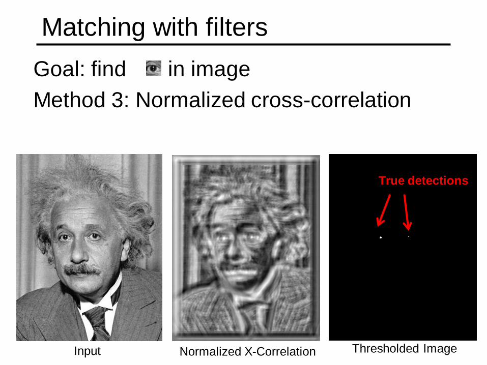
Matching with filters Goal: find in image Method 3: Normalized cross-correlation

Input Normalized X-Correlation Thresholded Image

True detections

Q: What is the best method to use? A: Depends Zero-mean filter: fastest but not a great

matcher SSD: next fastest, sensitive to overall

intensity Normalized cross-correlation: slowest,

invariant to local average intensity and contrast

Side by Derek Hoiem

point processing & filtering - university of …cs194-26/fa16/lectures/...point processing &...

Documents