point and prediction interval estimation for electricity markets with machine learning techniques...

Neurocomputing 118 (2013) 301–310

Contents lists available at SciVerse ScienceDirect

Neurocomputing

0925-23http://d

n CorrE-m

eez1080bijayake

journal homepage: www.elsevier.com/locate/neucom

Point and prediction interval estimation for electricity marketswith machine learning techniques and wavelet transforms

Nitin Anand Shrivastava n, Bijaya Ketan PanigrahiDepartment of Electrical Engineering, Indian Institute of Technology Delhi, New Delhi, India

a r t i c l e i n f o

Article history:Received 9 November 2012Received in revised form28 January 2013Accepted 6 February 2013
Communicated by Manoj Kumar Tiwari
uncertainty that prevails in the system. Due to a number of known, unknown factors, the electricity

Available online 9 May 2013

Keywords:Artificial neural network (ANN)BootstrapsExtreme learning machine (ELM)Prediction intervalsWavelet transformsUncertainty

12/$ - see front matter & 2013 Elsevier B.V. Ax.doi.org/10.1016/j.neucom.2013.02.039

esponding author. Tel.: +91 9540730864.ail addresses: [email protected],[email protected] (N. Anand Shrivastava),[email protected] (B. Ketan Panigrahi

a b s t r a c t

A growing number of countries all over the world are switching over to deregulated or the marketstructure of electricity sector with a view to enhance productivity, efficiency and to lower the prices.Barring a few cases, the deregulated structure is doing quite well in most of the countries. Howevera persistent issue that plagues the involved parties such as producers, traders, retailers etc., is the

prices exhibit fluctuating characteristics which is difficult to control as well as predict. Several forecastingtechniques have been developed and successfully implemented for existing markets around the worldwith comparable performance. However, the uncertainty aspect of the point forecasts has not beenanalyzed significantly. In this work, an attempt is made to quantify such uncertainties existing in themarket using statistical techniques like prediction intervals. Hybrid models using neural networks andExtreme Learning machines with wavelets as preprocessors are developed and applied for point as wellas prediction interval forecasting for Ontario Electricity Market, PJM Day-Ahead and Real time markets.

& 2013 Elsevier B.V. All rights reserved.

1. Introduction

Accurate forecasting of the market clearing prices in a pool typemarket structure is a vital necessity for a number of entities suchas market traders, power plant developers, generation companies,load serving entities and large industrial consumers etc.This necessity is driven by the need for appropriate decisionmaking for risk management. Suppliers are primarily interestedin optimal bidding strategies while consumers vouch for max-imum power with minimum expenses. A number of factors suchas fluctuating fuel costs, hydrological conditions, extreme seasonalvariations, network constraints and complex bidding strategies ofmarket players contribute to the wide fluctuations in the marketclearing prices. Capturing such wide fluctuations through differentforecasting techniques is an important as well as promising area ofresearch. Moreover the upcoming smart grid revolution whereadvance metering systems enable price responsive usage bycustomers, the problem of accurate price forecasting is becomingmore and more challenging.

Every year a number of novel techniques are being added to the listof attempts being made to forecast prices in the electricity markets.Some of the time series based techniques proposed by researchers

ll rights reserved.

).

include methodologies like dynamic regression and transfer func-tion [1], auto-regressive integrated moving average (ARIMA) [2],mixed ARIMA models [3] and generalized auto-regressive condi-tional heteroscedastic (GARCH) [4] etc. These approaches arebased on time series models which are linear predictors, whileelectricity price is generally a nonlinear function of its inputfeatures. So, the unusual traits of the price signal may not becompletely captured by the time series techniques [5].

Many tools have been developed based on artificial intelligencemethods which find a mapping between the input features andthe spot price. Generally, this mapping is performed on historicalexamples given to the network and these methods are simple andcomputationally efficient. Along these lines, researchers havesuggested artificial neural networks (NNs) [6–9], fuzzy NNs[10,11] and support vector machines (SVMs) [12] etc. for priceforecasting. Among the various methods, ANNs are quite wellrecognized and applied by the researchers. The appropriate selec-tion of input features is essential for the success of NN based priceforecast methods. Apart from that, the efficiency of these methodsusually depends on the correct tuning of their adjustable para-meters, e.g., the number of hidden layers, nodes, weights andtransfer function etc., of the NNs. Extreme Learning Machine(ELM) is a recently developed novel learning algorithm forsingle-hidden-layer feedforward neural networks (SLFN) [13,14].The distinguishing feature of this learning algorithm is that herethe input weights and hidden biases are randomly chosen, andthe output weights are analytically determined by using the

www.elsevier.com/locate/neucom

www.elsevier.com/locate/neucom

http://dx.doi.org/10.1016/j.neucom.2013.02.039



http://crossmark.dyndns.org/dialog/?doi=10.1016/j.neucom.2013.02.039&domain=pdf



mailto:[email protected]




N. Anand Shrivastava, B. Ketan Panigrahi / Neurocomputing 118 (2013) 301–310302

Moore-Penrose (MP) generalized inverse. The advantage of ELMover the traditional gradient-based learning algorithms is that itlearns much faster with a higher generalization performance andit also avoids the difficulties faced by gradient-based learningmethods such as learning rate, learning epochs, local minima,stopping criteria, and the over-tuning problems [15–17]. Theabilities of each of these techniques to estimate the future priceshas been proved in publications by many researchers. The estima-tion accuracies of these methods for different case studies acrossdifferent markets have been found to be consistently similar.For some cases one method is superior in some respect, while inanother case a different model is superior. However no singlemethod has been proven to be the best for all applications.

An important factor in applying these methodologies is thequantification of uncertainty bounds on their resultant estima-tions. The above mentioned techniques have been used essentiallyfor point predictions when supplied with a set of input data andsuch predictions are highly subject to a certain degree of uncer-tainty. A point forecast or output of a specific model is generallya single number which estimates the unknown true targetedvalue. Although deemed to be quite accurate, they give noinformation about the degree of uncertainty associated with theforecast. Although the research and application of machine learn-ing techniques particularly the Neural Networks are in full swing,still the performance of these techniques is likely to be unreliableand detrimental under uncertainty in the data. It has also beenverified by researchers that NN models are deterministic fromtheoretical considerations [18] and therefore their application in astochastic time series prediction is quite dubious. The electricityprice is a stochastic time series with very high uncertainty [2] andtherefore predicting the exact point value of electricity prices inthe future is quite a difficult task. The uncertainty in the output ofthe machine learning models is contributed either by the structureof the model or the inherent uncertainty in the data sets which isquite true for electricity prices. In order to quantify and representthe uncertainty of predictions, the commonly applied statisticaltools are Confidence Intervals (CIs) and Predictions Intervals (PIs).Confidence intervals are based on the accuracy of the prediction ofthe regression i.e., of the mean of the target probability distribu-tion. On the other hand, Prediction intervals take into account theaccuracy with which we are able to capture the actual targets [19].

Different methods have been proposed by the researchers in thepast for determination of prediction intervals. The primary ones arethe delta technique, the Bayesian technique and the Bootstraptechnique. The delta technique is based on the understanding thatmultilayer feedforward neural networks are basically non-linearregression models which can be linearized using Taylor's seriesexpansion [20]. In Bayesian technique, each parameter in a neuralnetwork is considered as a distribution rather than a single value andtherefore the network outcomes will also be in the form of distribu-tions conditional on the observed training set [18]. It suffers from thelimitation of massive computational burden and calculation ofHessian matrix. Bootstrap method [21–23] is the most well knownand applied method for construction of PIs for NN point forecast.Bootstrap method is basically a resampling technique which hasbeen found to be quite reliable compared to other techniques butdemands large computational cost for large data sets. Research basedon Prediction interval construction is gaining more and more interestnowadays. Some of the contemporary attempts are in fields relatedto bus travel time predictions [24], baggage handling systems [25,26],financial services [27], hydrological predictions [28]. Some of theworks related to energy markets are presented in [29,30].

In this work, we have made an attempt to construct predictionintervals for a day ahead price forecasting problem of the energymarkets. Bootstrapping method has been employed for thispurpose because it is efficient and easy to use in comparison to

Bayesian method involving complex computations. And it alsogives rise to input-dependent values for variance in comparison tothe delta method which makes a strong case for its relevance inconstructing reliable prediction intervals [31]. Different modelsbased on Neural network and Extreme Learning Machine areconstructed. Wavelet tool is employed to decompose the highlyfluctuating price series into different subseries for capturingdifferent frequency patterns in the historical data. The model istested for predicting hourly prices for the Ontario Electricitymarket and also PJM Day ahead and Real time markets. The restof the paper is organized as follows. Section 2 gives a introductionto the various modules of the complete model. The completemethodology and different case studies are presented in Section 3.The conclusions from the work are finally presented in Section 4.

2. Theory and background

2.1. Artificial neural network

A neural network is a model or a machine which tries to mimicthe complex task performance capability of the brain [32].It consists of neurons which are characterized by three essentialelements: the connection links represented by the weight orstrength of the connection, an adder, and an activation function.The function of the adder is to sum the input signals weighted bythe respective synapses, and the activation function limits theoutput of the neuron within a certain range. θ is an externalthreshold to suppress the net input of the activation function. Thefinal output is given by the following expression:

oj ¼ ϕ ∑n

i ¼ 1ðwijxi−θjÞ ð1Þ

A neural network performs an input–output mapping of a giventask with the help of a learning process. The learning processinvolves presentation of a set of examples to the network andsimultaneously the weights are adjusted to obtain a minimumerror. Finally, the knowledge acquired by the neural network istested by applying it to an unseen example. If the network is welltrained, then it should be able to generalize and give accurateoutput for the unseen example.

Amongst the different NN architectures, the FFNN architecture,which is also known as multilayer perceptron (MLP), along withback propagation (BP) as the learning algorithm is most popular.Researchers have verified that one hidden layer network withhidden nodes is capable of representing any functional relation-ship between input and output spaces [33]. A BP network withmulti/single hidden layer is basically a nonlinear transformationwhereas a network with no hidden layer is a linear regression model.

2.2. Extreme learning machines

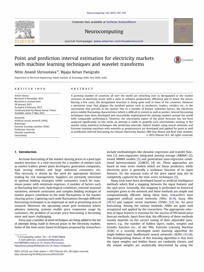
ELM is a single hidden-layer feedforward neural network (SLFN)which randomly chooses the input weight matrix W and analyti-cally determines the output weight matrix β of SLFN. Fig. 1 showsthe structure of a ELM model. Consider N arbitrary distinct samplesðxi; tiÞ where xi ¼ ½xi1; xi2;…; xin�T∈Rn and ti ¼ ½ti1; ti2;…; tim�T∈Rm.For this data, a standard SLFN with ~N hidden nodes and activationfunction g(x) can be mathematically modeled as [13]

∑~N

i ¼ 1βigiðxjÞ ¼ ∑

~N

i ¼ 1βigiðwixj þ bi ¼ yjÞ; j¼ 1…N ð2Þ

where wi ¼ ½wi1;wi2;…;win�T is the weight vector connecting theith hidden node and the input nodes, βi ¼ ½βi1; βi2;…; βim�T is theweight vector connecting the ith hidden node and the outputnodes, and bi is the threshold of the ith hidden node. The operation

Fig. 1. The structure of ELM model.

N. Anand Shrivastava, B. Ketan Panigrahi / Neurocomputing 118 (2013) 301–310 303

wi:xj in (2) denotes the inner product of wi and xj. If the standardSLFNs with ~N hidden nodes with activation function g(x) canapproximate these N samples with zero error, then we have

∑N

j ¼ 1∥yj−tj∥¼ 0 ð3Þ

where y is the actual output value of the SLFN. This implies theexistence of βi, wi and bi such that

∑~N

i ¼ 1βigiðwixj þ bi ¼ tjÞ; j¼ 1…N ð4Þ

The above N equations can be written compactly as

Hβ¼ T ð5Þwhere H is the hidden layer output matrix.

H ¼hðx1Þ…

hðxNÞ

264

375¼

h1ðx1Þ … h ~N ðx1Þ… … …

h1ðxNÞ … h ~N ðxNÞ

264

375 ð6Þ

β¼

βT1……βT~N

266664

377775 ð7Þ

T ¼

tT1……tT~N

266664

377775 ð8Þ

Unlike SLFN, in ELM the input weights and hidden biases arerandomly generated and do not require any tuning. The outputweights linking the hidden layer to the output layer can bedetermined in a similar fashion as finding the least-square solu-tion to the given linear system. The minimum norm least-square(LS) solution to the linear system (5) is

β ¼H†T ð9Þwhere H† is the is the Moore–Penrose generalized inverse ofmatrix H [34,35]. The solution thus obtained is unique andhas the minimum norm among all the LS solutions. By usingthe Moore–Penrose inverse method, ELM tends to obtain agood generalization performance with a radically increasedlearning speed.

2.3. Wavelet transforms

Wavelet transform is a mathematical tool used to extract therelevant time–frequency information from non-periodic and tran-sient signals. Wavelets functions disintegrate the data into

different frequency components, and then analyze each compo-nent with a resolution matched to its scale. Wavelet techniqueshave been developed independently in the domains of mathe-matics, quantum physics, electrical engineering and seismic geol-ogy [36]. Collaborative research in these fields during the last fewyears have led to many new wavelet applications such as imagecompression [37,38], texture classification [39], power quality [40],hydrological forecasting [41] and earthquake prediction [42].

The wavelet transform technique is implemented consideringa limited number of positions and resolution levels (discretewavelet transform). The wavelet transform separates out differentconstitutive series with more refined frequency patterns from thevolatile price series. The prospective behavior of these constitutiveseries is then predicted using different models and reverse wavelettransform is performed to generate the final price. The decom-position coefficients of the wavelet transform of the hourly priceseries determined by technique are given by [43]

pWmn ¼ 2−ðm=2Þ ∑T−1

t ¼ 0ptW

t−n � 2m

2m

� �

¼ 2−ðm=2Þ ∑T−1

t ¼ 0ptWmn tð Þ ð10Þ

where W �ð Þ is the selected wavelet function, pt is the value of theprice at hour t, T is the length of the series, pWmn is the decomposi-tion coefficient corresponding to position n and resolution level m.If the number of observations, T, is divisible by 2m, then thenumber of coefficients at each resolution level is T=2m. Calcula-tions can be made faster by treating expression (10) as a convolu-tion, and the efficient Fast Fourier Transform used, as stated in[44].

An effective way to opt for the wavelet functions is the multi-resolution technique based on using a father wavelet function andits complementary, a mother wavelet function. The father functionallows extracting the low frequency components of the series,while the mother one allows extracting high frequency compo-nents of the series. Moreover, it is better to choose orthogonalwavelet functions owing to their appropriate mathematical prop-erties. Hence, the “approximation series”, Amðm¼ 1;…;MÞ, and the“detail series”, Dmðm¼ 1;…;MÞ, are defined as

Am ¼∑npΦmnφmnðtÞ; m¼ 1;…;M ð11Þ

and

Dm ¼∑npΨmnψmnðtÞ; m¼ 1;…;M ð12Þ

where φmnðhÞ and ψmnðhÞ are the father andmother wavelet functions,and pΦmn and pΨmn are the coefficients obtained through (10).The expression of the original price series ptðt ¼ 1; ‥; TÞ can now bereconstructed by

pt ¼D1 þ⋯þ DM þ AM ð13Þwhich is the denominated multiresolution decomposition of the priceseries.

The most commonly used wavelets in different applications areDaubechies. The characteristics of these families of wavelets is thatthe smoothness increases with the order of the functions. Butsimultaneously the support intervals also increase, which maydeteriorate the prediction [45]. Therefore, low order waveletfunctions are generally advisable.

2.4. Construction of prediction intervals

Construction of prediction intervals through classical methodsis based on the assumption that the underlying distribution of theerror process is known. The most widely used technique is that ofBox–Jenkins [46] which relies on standard normal distribution.


This assumption does not stand valid in practical situations.Therefore prediction intervals constructed under such assump-tions are likely to produce poor results [47]. Bootstrapping isa computer based statistical technique proposed by Efron [48]which is meant to approximate the unknown probability distribu-tion of an estimator or statistic by an empirical distributionobtained by a resampling process. They are being employed byresearchers for improving the accuracy of the statistical estima-tions. Bootstrap methods, which are non-parametric alternative toconventional methods, are designed to produce asymptoticallycorrect coverage rates under no specific assumption about theerror distribution. Consider Fk(x) as the unconditional distributionfunction of the random variable ytþk. Had the distribution functionFk(x) been known to us, then the theoretical prediction intervalconstructed at time t þ k would be

ytþk þ F−1kβ

2

� �; ytþk þ F−1k 1−

β

2

� �� ð14Þ

where

F−1k ðpÞ ¼ inf fxjFkðxÞ≥pgIn real life problems, the distribution is not apriori known to us.

An alternative approach is to use the bootstrap methods and thenplug in the quantiles in (14) and get the bootstrap predictionintervals. The structure for all bootstrap based methods remainsalmost the same with a slight difference in the resampling methodused. One of the approaches for bootstrapping was proposed byStine [49] for time series approach. An adaption of the proposedapproach for machine learning techniques goes as follows.

(1)
Randomly draw B independent bootstrap sample from thetraining data set.
(2)
Perform function approximation using ML techniques. Deter-mine the residuals.
(3)
Draw new residuals randomly with replacement from there-centered and re-scaled distribution function of the residuals.
(4)
Construct new bootstrap samples by adding the randomlydrawn residuals to the previous function approximations.
(5)
Retrain the models with new data sets and predict the futurepoints.
(6)
Repeat the process for different bootstrap analogs and deter-mine prediction intervals.
The disadvantage of this approach is that it results in thereplication of the random mechanism of parameter estimation andnot on the actual conditional distribution of the predicted valuegiven the observed dataset [47]. An alternative approach wassuggested by Thombs and Schucany [50] where the issue of theconditional distribution of the future value with given observedvalues is adequately addressed. In this case, the observed data setis kept fixed and centered, re-scaled residuals are determined.New bootstrap replications are constructed using random valuesdrawn from the empirical distribution of the residuals.The replicated series is fitted using ML technique and newparameters are estimated. Forward bootstrap errors are now againdrawn from the empirical distribution of errors and forwardbootstrap realizations are now constructed. For a given datasetfxi; yigni ¼ 1, the targets can be modeled as

yi ¼ gðxiÞ þ εi ð15Þwhere yi is the ith target and εi is the error which is a randomvariable with zero expectation and finite variance s2ε . In practice,the estimate of the true regression mean is obtained by the modelgðxiÞ. Now, for the given set of data, confidence intervals can bedefined as the measures of uncertainty between the true regres-sion gðxiÞ and its estimate gðxiÞ. In practical applications, we are

not just concerned with the variance of the model output withrespect to its unknown true regression mean, rather we are moreinterested in the probability of the actual targeted variable beingtracked by the model. This kind of uncertainty is quantified by theterm Prediction interval which focusses on the distribution of thequantity yi−gðxiÞ.

The error variable εi can be approximated as

εi ¼ yi−gðxiÞ ð16Þ

The errors are centered, re-scaled and an empirical distributionis constructed for them in order to avoid a systematic error inbootstrapping. Draw new errors randomly with replacement fromthe re-centered and re-scaled distribution function of the errorsand construct a new bootstrap sample by adding it to thepredicted results. Therefore the new bootstrap data sample canbe given as

yn

i ¼ gðxiÞ þ ~εni ð17Þ

where ~εni is the randomly drawn error with uniform probabilitydistribution from the centered and rescaled error vector ~ε.

B number of bootstrap replicates are formed in a similarmanner. For a large number of bootstrap replications, the predic-tion intervals can be constructed by using the quantiles of thebootstrap sampling distribution of the estimator. In order toconstruct 100ð1−αÞ% prediction intervals, the output of B boot-strap replicates are ordered and corresponding lower ðBα=2Þ andupper ðBð1−α=2ÞÞ quantiles can be plugged in for individual targetobservations.

2.5. Forecast error measures

The prediction performance of the models is assessed bydifferent statistical measures or indices [51]. The most commonlyused indices are based on absolute errors i.e. absolute values ofdifferences between the actual price, P, and predicted price, P , fora given hour, h. The Mean Absolute Error (MAE) and MeanAbsolute Percentage Error (MAPE) are typical examples of mostwidely referred indices in the literature.The daily MAPE can beexpressed as

MAPE¼ 1N

∑N

h ¼ 1

jPh−Ph jPh

ð18Þ

It is evident from the formulae that the error has been normalizedusing the actual price at that hour. This is necessary in order tocompare the indices for distinct data sets. This index works wellfor load forecasting where the load values are quite large and theload series does not exhibit wide fluctuations. Contrary to loads,the electricity price series is subject to spikes or outliers.The outliers greatly affect the distribution of the prices making itmore and more skewed. In such situations, median is consideredto be a better measure of the central tendency rather than themean. Median is more effective in combating outliers (or spikes)and therefore the median price can also be used for normalization.The resulting measure is termed as Median Daily Error (MeDE):

MeDE¼ 1N

∑N

h ¼ 1

jPh−Ph j~P24

ð19Þ

where ~P24 is the median price obtained during the day.In order to asses the performance of the prediction intervals, two

different accuracy measures are commonly used. An importantrequirement from the prediction intervals is their ability to capturethe actual target variables. This is termed as the Prediction intervalcoverage probability (PICP) which can be mathematically expressed

253035404550556065

PRICE($\MWh)

Ontario


as

PICP¼ 1N

∑N

i ¼ 1Ci

where Ci ¼1 ti∈½Li;Ui�0 ti∉½Li;Ui�

(ð20Þ

where N is the number of samples in the test set, and Li and Ui arelower and upper bounds of the ith PI respectively. Very high PICP canbe easily achieved in case the width of the prediction intervals is large.But large PI's have higher level of uncertainty associated with themand are not very practically useful. Therefore another importantassessment of the prediction intervals has to be done throughevaluation of the mean prediction interval width (MPIW) [30]:

MPIW ¼ 1N

∑N

i ¼ 1ðUi−LiÞ ð21Þ

If we are interested in comparing the MPIW index acrossdifferent data sets, then it has to be normalized by the range ofthe corresponding data set. The new index is termed as Normal-ized Mean Prediction Interval Width (NMPIW):

NMPIW ¼ MPIWRange

ð22Þ

Both the indices mentioned above are conflicting in nature.An increase in NMPIW will reflect in higher PICP and vice-versa.What is required by a suitable decision maker is a small NMPIWand high PICP. Independent assessment of these measures is not ofmuch help. Therefore, a comprehensive index consisting of bothPICP and NMPIW is suggested by Khosravi et al. [52]. The CoverageWidth Criterion (CWC) is expressed as

CWC¼NMPIWð1þ γðPICPÞeð−ηðPICP−μÞÞÞ

where γðPICPÞ is given by γ ¼0 PICP≥μ1 PICPoμ

(ð23Þ

where η and μ refers to the hyperparameters controlling themagnitude of CWC index. μ is the nominal confidence level forwhich the intervals are constructed. The index is constructed suchthat violation of the nominal coverage probability limit is pena-lized more prominently compared to higher widths if such viola-tions exist. If the coverage probability is close to normal, then it isthe interval width which dominates the magnitude of CWC.

2.6. Steps of the proposed methodology

The specific steps of the point and interval forecasting meth-odology used here are as follows:

0 20 40 60 80 100 120 140 160 1801520

(1)

HOUR

Select a suitable training period from the historical dataavailable at hand.

(2)
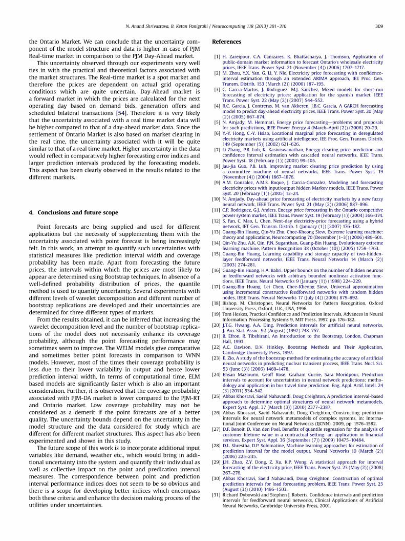
Fig. 2. Weekly price profile of Ontario market.
Perform wavelet decomposition of the selected time series ofelectricity prices till the desired level.

(3)

160

Create separate training and testing data sets for eachindividual decomposed wavelet subseries. Normalize thetraining and testing sets.

140
(4)
120h)

Perform function approximation with the training data usingthe machine learning models and determine the residuals.

100

W
(5)
E($\M

Randomly draw residuals with replacement from thecentered and rescaled distribution of the residuals.

80

IC
(6) 60PR
Add the randomly drawn residuals to the previous functionapproximations and create new bootstrap data.

40
(7)
0 20 40 60 80 100 120 140 160 18020

HOUR

Fig. 3. Weekly price profiles of PJM market.

Retrain the models with the new bootstrap data and predictfuture points for the unseen testing data correspondingto individual decomposed wavelet series. Perform waveletreconstruction to get the normal price forecast for thenext hour.

(8)
Repeat steps 5–7 for all the bootstrap samples. (9) Plug in the required quantiles in the empirical distribution of
the bootstrap outputs and determine the prediction intervals.The mean of the bootstrap outputs is taken as the approx-imate point forecast of the corresponding hour.

(10)
Repeat the process for the next hour.
3. Case studies and experimental results

This section presents a detailed description of the case studiespertaining to different electricity market structures using theproposed methodology

3.1. Market description

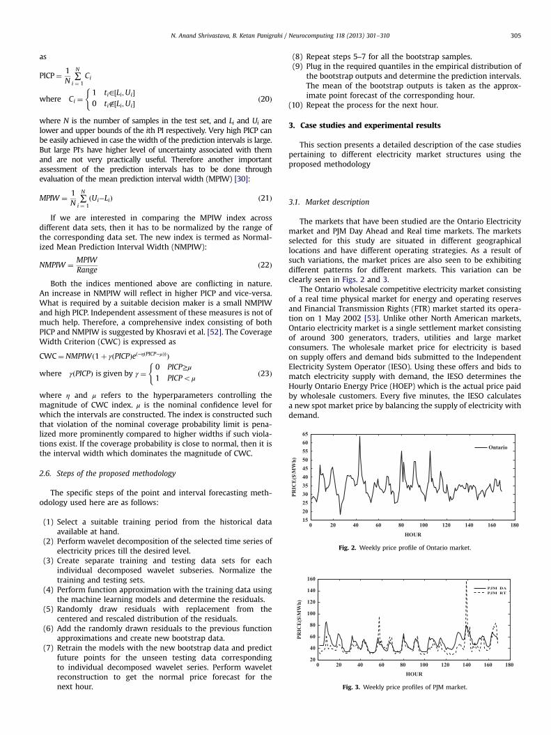
The markets that have been studied are the Ontario Electricitymarket and PJM Day Ahead and Real time markets. The marketsselected for this study are situated in different geographicallocations and have different operating strategies. As a result ofsuch variations, the market prices are also seen to be exhibitingdifferent patterns for different markets. This variation can beclearly seen in Figs. 2 and 3.

The Ontario wholesale competitive electricity market consistingof a real time physical market for energy and operating reservesand Financial Transmission Rights (FTR) market started its opera-tion on 1 May 2002 [53]. Unlike other North American markets,Ontario electricity market is a single settlement market consistingof around 300 generators, traders, utilities and large marketconsumers. The wholesale market price for electricity is basedon supply offers and demand bids submitted to the IndependentElectricity System Operator (IESO). Using these offers and bids tomatch electricity supply with demand, the IESO determines theHourly Ontario Energy Price (HOEP) which is the actual price paidby wholesale customers. Every five minutes, the IESO calculatesa new spot market price by balancing the supply of electricity withdemand.

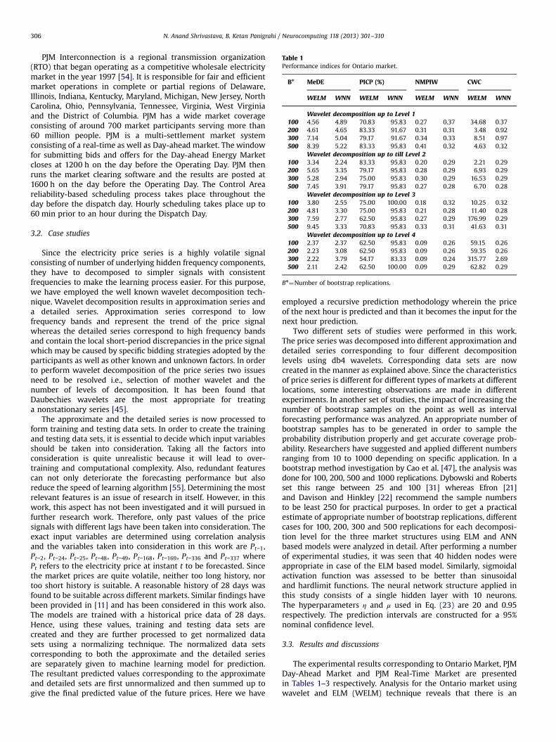
Table 1Performance indices for Ontario market.

Bn MeDE PICP (%) NMPIW CWC

WELM WNN WELM WNN WELM WNN WELM WNN

Wavelet decomposition up to Level 1100 4.56 4.89 70.83 95.83 0.27 0.37 34.68 0.37200 4.61 4.65 83.33 91.67 0.31 0.31 3.48 0.92300 7.14 5.04 79.17 91.67 0.34 0.33 8.51 0.97500 8.39 5.22 83.33 95.83 0.41 0.32 4.63 0.32

Wavelet decomposition up to till Level 2100 3.34 2.24 83.33 95.83 0.20 0.29 2.21 0.29200 5.65 3.35 79.17 95.83 0.28 0.29 6.93 0.29300 5.28 2.94 75.00 95.83 0.30 0.29 16.53 0.29500 7.45 3.91 79.17 95.83 0.27 0.28 6.70 0.28



Bn¼Number of bootstrap replications.


PJM Interconnection is a regional transmission organization(RTO) that began operating as a competitive wholesale electricitymarket in the year 1997 [54]. It is responsible for fair and efficientmarket operations in complete or partial regions of Delaware,Illinois, Indiana, Kentucky, Maryland, Michigan, New Jersey, NorthCarolina, Ohio, Pennsylvania, Tennessee, Virginia, West Virginiaand the District of Columbia. PJM has a wide market coverageconsisting of around 700 market participants serving more than60 million people. PJM is a multi-settlement market systemconsisting of a real-time as well as Day-ahead market. The windowfor submitting bids and offers for the Day-ahead Energy Marketcloses at 1200 h on the day before the Operating Day. PJM thenruns the market clearing software and the results are posted at1600 h on the day before the Operating Day. The Control Areareliability-based scheduling process takes place throughout theday before the dispatch day. Hourly scheduling takes place up to60 min prior to an hour during the Dispatch Day.

3.2. Case studies

Since the electricity price series is a highly volatile signalconsisting of number of underlying hidden frequency components,they have to decomposed to simpler signals with consistentfrequencies to make the learning process easier. For this purpose,we have employed the well known wavelet decomposition tech-nique. Wavelet decomposition results in approximation series anda detailed series. Approximation series correspond to lowfrequency bands and represent the trend of the price signalwhereas the detailed series correspond to high frequency bandsand contain the local short-period discrepancies in the price signalwhich may be caused by specific bidding strategies adopted by theparticipants as well as other known and unknown factors. In orderto perform wavelet decomposition of the price series two issuesneed to be resolved i.e., selection of mother wavelet and thenumber of levels of decomposition. It has been found thatDaubechies wavelets are the most appropriate for treatinga nonstationary series [45].

The approximate and the detailed series is now processed toform training and testing data sets. In order to create the trainingand testing data sets, it is essential to decide which input variablesshould be taken into consideration. Taking all the factors intoconsideration is quite unrealistic because it will lead to over-training and computational complexity. Also, redundant featurescan not only deteriorate the forecasting performance but alsoreduce the speed of learning algorithm [55]. Determining the mostrelevant features is an issue of research in itself. However, in thiswork, this aspect has not been investigated and it will pursued infurther research work. Therefore, only past values of the pricesignals with different lags have been taken into consideration. Theexact input variables are determined using correlation analysisand the variables taken into consideration in this work are Pt−1,Pt−2, Pt−24, Pt−25, Pt−48, Pt−49, Pt−168, Pt−169, Pt−336 and Pt−337 wherePt refers to the electricity price at instant t to be forecasted. Sincethe market prices are quite volatile, neither too long history, nortoo short history is suitable. A reasonable history of 28 days wasfound to be suitable across different markets. Similar findings havebeen provided in [11] and has been considered in this work also.The models are trained with a historical price data of 28 days.Hence, using these values, training and testing data sets arecreated and they are further processed to get normalized datasets using a normalizing technique. The normalized data setscorresponding to both the approximate and the detailed seriesare separately given to machine learning model for prediction.The resultant predicted values corresponding to the approximateand detailed sets are first unnormalized and then summed up togive the final predicted value of the future prices. Here we have

employed a recursive prediction methodology wherein the priceof the next hour is predicted and than it becomes the input for thenext hour prediction.

Two different sets of studies were performed in this work.The price series was decomposed into different approximation anddetailed series corresponding to four different decompositionlevels using db4 wavelets. Corresponding data sets are nowcreated in the manner as explained above. Since the characteristicsof price series is different for different types of markets at differentlocations, some interesting observations are made in differentexperiments. In another set of studies, the impact of increasing thenumber of bootstrap samples on the point as well as intervalforecasting performance was analyzed. An appropriate number ofbootstrap samples has to be generated in order to sample theprobability distribution properly and get accurate coverage prob-ability. Researchers have suggested and applied different numbersranging from 10 to 1000 depending on specific application. In abootstrap method investigation by Cao et al. [47], the analysis wasdone for 100, 200, 500 and 1000 replications. Dybowski and Robertsset this range between 25 and 100 [31] whereas Efron [21]and Davison and Hinkley [22] recommend the sample numbersto be least 250 for practical purposes. In order to get a practicalestimate of appropriate number of bootstrap replications, differentcases for 100, 200, 300 and 500 replications for each decomposi-tion level for the three market structures using ELM and ANNbased models were analyzed in detail. After performing a numberof experimental studies, it was seen that 40 hidden nodes wereappropriate in case of the ELM based model. Similarly, sigmoidalactivation function was assessed to be better than sinusoidaland hardlimit functions. The neural network structure applied inthis study consists of a single hidden layer with 10 neurons.The hyperparameters η and μ used in Eq. (23) are 20 and 0.95respectively. The prediction intervals are constructed for a 95%nominal confidence level.

3.3. Results and discussions

The experimental results corresponding to Ontario Market, PJMDay-Ahead Market and PJM Real-Time Market are presentedin Tables 1–3 respectively. Analysis for the Ontario market usingwavelet and ELM (WELM) technique reveals that there is an

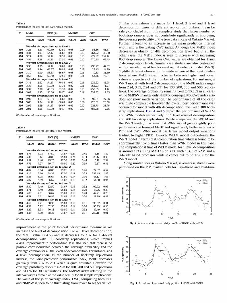
Table 2Performance indices for PJM-Day Ahead market.








Table 3Performance indices for PJM-Real Time market.








0 5 10 15 20 2520

25

30

35

40

45

50

55

60

Hour

Price($/MWh)

Fig. 4. Actual and forecasted daily profile of HOEP with WELM.

0 5 10 15 20 2520

25

30

35

40

45

50

55

Hour

HOEP($/MWh)

Fig. 5. Actual and forecasted daily profile of HOEP with WNN.


improvement in the point forecast performance measure as weincrease the level of decomposition. For a 1 level decomposition,the MeDE value is 4.56 and it decreases to 2.37 for a 4-leveldecomposition with 100 bootstrap replications, which impliesa 48% improvement in performance. It is also seen that there is nopositive correspondence between the coverage probability and thecoverage criterion for all the levels of decomposition. For instance, at a4 level decomposition, as the number of bootstrap replicationsincrease, the Point prediction performance index, MeDE, decreasesgradually from 2.37 to 2.11 which is quite desirable. However, thecoverage probability sticks to 62.5% for 100, 200 and 500 replicationsand 54.17% for 300 replications. The NMPIW index referring to theinterval widths remain at the value of 0.09 for all samples/replications.The value of the joint coverage index, CWC, comprising both PICPand NMPIW is seen to be fluctuating from lower to higher values.

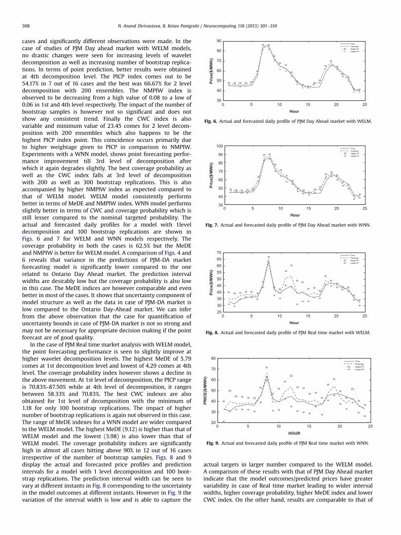
Similar observations are made for 1 level, 2 level and 3 leveldecomposition cases for different replication numbers. It can besafely concluded from this complete study that larger number ofbootstrap samples does not contribute significantly in improvingthe coverage probability of the true data in case of Ontario Market.Further, it leads to an increase in the mean prediction intervalwidth and a fluctuating CWC index. Although the MeDE indexdecreases gradually for 4th decomposition level, but in all theother cases, the MeDE index is seen to increase with increasingBootstrap samples. The lower CWC values are obtained for 1 and2 decomposition levels. Similar case studies are also performedwith a wavelet based feedforward neural network model (WNN).Slightly different observation is made in case of the point predic-tions where MeDE index fluctuates between higher and lowervalues irrespective of the number of replications. For instance, aWNN model with level 2 decomposition, the MeDE index rangesfrom 2.24, 3.35, 2.94 and 3.91 for 100, 200, 300 and 500 replica-tions. The coverage probability remains fixed to 95.83% in all caseswhile NMPIW changes only slightly. Consequently, CWC index alsodoes not show much variation. The performance of all the caseswas quite comparable however the overall best performance wasobtained for model with 4th decomposition level with 100 boot-strap replications. Figs. 4 and 5 depict the performance of WELMand WNN models respectively for 1 level wavelet decompositionand 200 bootstrap replications. While comparing the WELM andthe WNN model, it is seen that WNN model gives slightly poorperformance in terms of MeDE and significantly better in terms ofPICP and CWC. WNN model has larger model output variationsleading to higher PICP. However WELM model outperforms theWNN model in terms of its computation time which is found to beapproximately 10–15 times faster than WNN model in this case.The computational time of WELM model for 1 level decompositionis around 133 s using MATLAB on a PC with 16 GB of RAM and a3.4-GHz based processor while it comes out to be 1790 s for theWNN model.

Along similar lines as Ontario Market, several case studies wereperformed on the PJM market, both for Day-Ahead and Real-time

0 5 10 15 20 2530

40

50

60

70

80

90

Hour

Price($/MWh)

Fig. 6. Actual and forecasted daily profile of PJM Day Ahead market with WELM.

0 5 10 15 20 2530

40

50

60

70

80

90

100

HourPrice($/MWh)

Fig. 7. Actual and forecasted daily profile of PJM Day Ahead market with WNN.

0 5 10 15 20 2525303540455055606570

Hour

Price($/MWh)

Fig. 8. Actual and forecasted daily profile of PJM Real time market with WELM.

0 5 10 15 20 2520

30

40

50

60

70

80

HOUR

PRICE($/MWh)

Fig. 9. Actual and forecasted daily profile of PJM Real time market with WNN.


cases and significantly different observations were made. In thecase of studies of PJM Day ahead market with WELM models,no drastic changes were seen for increasing levels of waveletdecomposition as well as increasing number of bootstrap replica-tions. In terms of point prediction, better results were obtainedat 4th decomposition level. The PICP index comes out to be54.17% in 7 out of 16 cases and the best was 66.67% for 2 leveldecomposition with 200 ensembles. The NMPIW index isobserved to be decreasing from a high value of 0.08 to a low of0.06 in 1st and 4th level respectively. The impact of the number ofbootstrap samples is however not so significant and does notshow any consistent trend. Finally the CWC index is alsovariable and minimum value of 23.45 comes for 2 level decom-position with 200 ensembles which also happens to be thehighest PICP index point. This coincidence occurs primarily dueto higher weightage given to PICP in comparison to NMPIW.Experiments with a WNN model, shows point forecasting perfor-mance improvement till 3rd level of decomposition afterwhich it again degrades slightly. The best coverage probability aswell as the CWC index falls at 3rd level of decompositionwith 200 as well as 300 bootstrap replications. This is alsoaccompanied by higher NMPIW index as expected compared tothat of WELM model. WELM model consistently performsbetter in terms of MeDE and NMPIW index. WNN model performsslightly better in terms of CWC and coverage probability which isstill lesser compared to the nominal targeted probability. Theactual and forecasted daily profiles for a model with 1leveldecomposition and 100 bootstrap replications are shown inFigs. 6 and 7 for WELM and WNN models respectively. Thecoverage probability in both the cases is 62.5% but the MeDEand NMPIW is better for WELMmodel. A comparison of Figs. 4 and6 reveals that variance in the predictions of PJM-DA marketforecasting model is significantly lower compared to the onerelated to Ontario Day Ahead market. The prediction intervalwidths are desirably low but the coverage probability is also lowin this case. The MeDE indices are however comparable and evenbetter in most of the cases. It shows that uncertainty component ofmodel structure as well as the data in case of PJM-DA market islow compared to the Ontario Day-Ahead market. We can inferfrom the above observation that the case for quantification ofuncertainty bounds in case of PJM-DA market is not so strong andmay not be necessary for appropriate decision making if the pointforecast are of good quality.

In the case of PJM Real time market analysis with WELM model,the point forecasting performance is seen to slightly improve athigher wavelet decomposition levels. The highest MeDE of 5.79comes at 1st decomposition level and lowest of 4.29 comes at 4thlevel. The coverage probability index however shows a decline inthe above movement. At 1st level of decomposition, the PICP rangeis 70.83%–87.50% while at 4th level of decomposition, it rangesbetween 58.33% and 70.83%. The best CWC indexes are alsoobtained for 1st level of decomposition with the minimum of1.18 for only 100 bootstrap replications. The impact of highernumber of bootstrap replications is again not observed in this case.The range of MeDE indexes for a WNN model are wider comparedto the WELMmodel. The highest MeDE (9.12) is higher than that ofWELM model and the lowest (3.98) is also lower than that ofWELM model. The coverage probability indices are significantlyhigh in almost all cases hitting above 90% in 12 out of 16 casesirrespective of the number of bootstrap samples. Figs. 8 and 9display the actual and forecasted price profiles and predictionintervals for a model with 1 level decomposition and 100 boot-strap replications. The prediction interval width can be seen tovary at different instants in Fig. 8 corresponding to the uncertaintyin the model outcomes at different instants. However in Fig. 9 thevariation of the interval width is low and is able to capture the

actual targets in larger number compared to the WELM model.A comparison of these results with that of PJM Day Ahead marketindicate that the model outcomes/predicted prices have greatervariability in case of Real time market leading to wider intervalwidths, higher coverage probability, higher MeDE index and lowerCWC index. On the other hand, results are comparable to that of


the Ontario Market. We can conclude that the uncertainty com-ponent of the model structure and data is higher in case of PJMReal-time market in comparison to the PJM Day-Ahead market.

This uncertainty observed through our experiments very wellties in with the practical and theoretical factors associated withthe market structures. The Real-time market is a spot market andtherefore the prices are dependent on actual grid operatingconditions which are quite uncertain. Day-Ahead market isa forward market in which the prices are calculated for the nextoperating day based on demand bids, generation offers andscheduled bilateral transactions [54]. Therefore it is very likelythat the uncertainty associated with a real time market data willbe higher compared to that of a day-ahead market data. Since thesettlement of Ontario Market is also based on market clearing inthe real time, the uncertainty associated with it will be quitesimilar to that of a real time market. Higher uncertainty in the datawould reflect in comparatively higher forecasting error indices andlarger prediction intervals produced by the forecasting models.This aspect has been clearly observed in the results related to thedifferent markets.

4. Conclusions and future scope

Point forecasts are being supplied and used for differentapplications but the necessity of supplementing them with theuncertainty associated with point forecast is being increasinglyfelt. In this work, an attempt to quantify such uncertainties withstatistical measures like prediction interval width and coverageprobability has been made. Apart from forecasting the futureprices, the intervals within which the prices are most likely toappear are determined using Bootstrap techniques. In absence of awell-defined probability distribution of prices, the quantilemethod is used to quantify uncertainty. Several experiments withdifferent levels of wavelet decomposition and different number ofbootstrap replications are developed and their uncertainties aredetermined for three different types of markets.

From the results obtained, it can be inferred that increasing thewavelet decomposition level and the number of bootstrap replica-tions of the model does not necessarily enhance its coverageprobability, although the point forecasting performance maysometimes seem to improve. The WELM models give comparativeand sometimes better point forecasts in comparison to WNNmodels. However, most of the times their coverage probability isless due to their lower variability in output and hence lowerprediction interval width. In terms of computational time, ELMbased models are significantly faster which is also an importantconsideration. Further, it is observed that the coverage probabilityassociated with PJM-DA market is lower compared to the PJM-RTand Ontario market. Low coverage probability may not beconsidered as a demerit if the point forecasts are of a betterquality. The uncertainty bounds depend on the uncertainty in themodel structure and the data considered for study which aredifferent for different market structures. This aspect has also beenexperimented and shown in this study.

The future scope of this work is to incorporate additional inputvariables like demand, weather etc., which would bring in addi-tional uncertainty into the system, and quantify their individual aswell as collective impact on the point and predication intervalmeasures. The correspondence between point and predictioninterval performance indices does not seem to be so obvious andthere is a scope for developing better indices which encompassboth these criteria and enhance the decision making process of theutilities under uncertainties.

References

[1] H. Zareipour, C.A. Canizares, K. Bhattacharya, J. Thomson, Application ofpublic-domain market information to forecast Ontario's wholesale electricityprices, IEEE Trans. Power Syst. 21 (November (4)) (2006) 1707–1717.

[2] M. Zhou, Y.X. Yan, G. Li, Y. Nie, Electricity price forecasting with confidence-interval estimation through an extended ARIMA approach, IEE Proc. Gen.Transm. Distrib. 153 (March (2)) (2006) 187–195.

[3] C. Garcia-Martos, J. Rodriguez, M.J. Sanchez, Mixed models for short-runforecasting of electricity prices: application for the spanish market, IEEETrans. Power Syst. 22 (May (2)) (2007) 544–552.

[4] R.C. Garcia, J. Contreras, M. van Akkeren, J.B.C. Garcia, A GARCH forecastingmodel to predict day-ahead electricity prices, IEEE Trans. Power Syst. 20 (May(2)) (2005) 867–874.

[5] N. Amjady, M. Hemmati, Energy price forecasting—problems and proposalsfor such predictions, IEEE Power Energy 4 (March–April (2)) (2006) 20–29.

[6] Y.-Y. Hong, C.-Y. Hsiao, Locational marginal price forecasting in deregulatedelectricity markets using artificial intelligence, IEE Proc. Gen. Transm. Distrib.149 (September (5)) (2002) 621–626.

[7] Li Zhang, P.B. Luh, K. Kasiviswanathan, Energy clearing price prediction andconfidence interval estimation with cascaded neural networks, IEEE Trans.Power Syst. 18 (February (1)) (2003) 99–105.

[8] Jau-Jia Guo, P.B. Luh, Improving market clearing price prediction by usinga committee machine of neural networks, IEEE Trans. Power Syst. 19(November (4)) (2004) 1867–1876.

[9] A.M. Gonzalez, A.M.S. Roque, J. Garcia-Gonzalez, Modeling and forecastingelectricity prices with input/output hidden Markov models, IEEE Trans. PowerSyst. 20 (February (1)) (2005) 13–24.

[10] N. Amjady, Day-ahead price forecasting of electricity markets by a new fuzzyneural network, IEEE Trans. Power Syst. 21 (May (2)) (2006) 887–896.

[11] C.P. Rodriguez, G.J. Anders, Energy price forecasting in the Ontario competitivepower systemmarket, IEEE Trans. Power Syst. 19 (February (1)) (2004) 366–374.

[12] S. Fan, C. Mao, L. Chen, Next-day electricity-price forecasting using a hybridnetwork, IET Gen. Transm. Distrib. 1 (January (1)) (2007) 176–182.

[13] Guang-Bin Huang, Qin-Yu Zhu, Chee-Kheong Siew, Extreme learning machine:theory and applications, Neurocomputing 70 (December (1–3)) (2006) 489–501.

[14] Qin-Yu Zhu, A.K. Qin, P.N. Suganthan, Guang-Bin Huang, Evolutionary extremelearning machine, Pattern Recognition 38 (October (10)) (2005) 1759–1763.

[15] Guang-Bin Huang, Learning capability and storage capacity of two-hidden-layer feedforward networks, IEEE Trans. Neural Networks 14 (March (2))(2003) 274–281.

[16] Guang-Bin Huang, H.A. Babri, Upper bounds on the number of hidden neuronsin feedforward networks with arbitrary bounded nonlinear activation func-tions, IEEE Trans. Neural Networks 9 (January (1)) (1998) 224–229.

[17] Guang-Bin Huang, Lei Chen, Chee-Kheong Siew, Universal approximationusing incremental constructive feedforward networks with random hiddennodes, IEEE Trans. Neural Networks 17 (July (4)) (2006) 879–892.

[18] Bishop, M. Christopher, Neural Networks for Pattern Recognition, OxfordUniversity Press, Oxford, U.K., USA, 1996.

[19] Tom Heskes, Practical Confidence and Prediction Intervals, Advances in NeuralInformation Processing Systems 9, MIT Press, 1997, pp. 176–182.

[20] J.T.G. Hwang, A.A. Ding, Prediction intervals for artificial neural networks,J. Am. Stat. Assoc. 92 (August) (1997) 748–757.

[21] B. Efron, R. Tibshirani, An Introduction to the Bootstrap, London, ChapmanHall, 1993.

[22] A.C. Davison, D.V. Hinkley, Bootstrap Methods and Their Application,Cambridge University Press, 1997.

[23] E. Zio, A study of the bootstrap method for estimating the accuracy of artificialneural networks in predicting nuclear transient process, IEEE Trans. Nucl. Sci.53 (June (3)) (2006) 1460–1478.

[24] Ehsan Mazloumi, Geoff Rose, Graham Currie, Sara Moridpour, Predictionintervals to account for uncertainties in neural network predictions: metho-dology and application in bus travel time prediction, Eng. Appl. Artif. Intell. 24(3) (2011) 534–542.

[25] Abbas Khosravi, Saeid Nahavandi, Doug Creighton, A prediction interval-basedapproach to determine optimal structures of neural network metamodels,Expert Syst. Appl. 37 (March (3)) (2010) 2377–2387.

[26] Abbas Khosravi, Saeid Nahavandi, Doug Creighton, Constructing predictionintervals for neural network metamodels of complex systems, in: Interna-tional Joint Conference on Neural Networks (IJCNN), 2009, pp. 1576–1582.

[27] D.F. Benoit, D. Van den Poel, Benefits of quantile regression for the analysis ofcustomer lifetime value in a contractual setting: an application in financialservices, Expert Syst. Appl. 36 (September (7)) (2009) 10475–10484.

[28] D.L. Shrestha, D.P. Solomatine, Machine learning approaches for estimation ofprediction interval for the model output, Neural Networks 19 (March (2))(2006) 225–235.

[29] J.H. Zhao, Z.Y. Dong, Z. Xu, K.P. Wong, A statistical approach for intervalforecasting of the electricity price, IEEE Trans. Power Syst. 23 (May (2)) (2008)267–276.

[30] Abbas Khosravi, Saeid Nahavandi, Doug Creighton, Construction of optimalprediction intervals for load forecasting problem, IEEE Trans. Power Syst. 25(August (3)) (2010) 1496–1503.

[31] Richard Dybowski and Stephen J. Roberts, Confidence intervals and predictionintervals for feedforward neural networks, Clinical Applications of ArtificialNeural Networks, Cambridge University Press, 2001.

http://refhub.elsevier.com/S0925-2312(13)00426-8/sbref1










































































[32] P. Claudia, Rodriguez, George J. Anders, Energy price forecasting in the Ontariocompetitive power system market, IEEE Trans. Power Syst. 19 (February (1))(2004) 366–374.

[33] K. Hornik, M. Stinchcombe, H. White, Multilayer feedforward networks areuniversal approximators, Neural Networks 2 (July (5)) (1989) 359–366.

[34] D. Serre, Matrices: Theory and Applications, New York, Springer, 2002.[35] C.R. Rao, S.K. Mitra, Generalized Inverse of Matrices and its Applications,

New York, John Wiley, 1971.[36] Lokenath Debnath, Wavelet Transforms and their Applications, PINSA-A, 64, A,

No. 6, November 1998, pp. 685–713.[37] Hoon Yoo, Jechang Jeong, Signal-dependent wavelet transform and applica-

tion to lossless image compression, Electron. Lett. 38 (February (4)) (2002)170–172.

[38] Macarena Boix, Begona Canto, Wavelet transform application to the compres-sion of images, Math. Comput. Model. 52 (October (7–8)) (2010) 1265–1270.

[39] Yu-Long Qiao, Chun-Hui Zhao, Chun-Yan Song, Complex wavelet based textureclassification, Neurocomputing 72 (October (16–18)) (2009) 3957–3963.

[40] K. Manimala, K. Selvi, R. Ahila, Optimization techniques for improving powerquality data mining using wavelet packet based support vector machine,Neurocomputing 77 (February (1)) (2012) 36–47.

[41] R. Maheswaran, Rakesh Khosa, Comparative study of different wavelets forhydrologic forecasting, Comput. Geosci. 46 (September) (2012) 284–295.

[42] Frederik J. Simons, Ben D.E. Dando, Richard M. Allen, Automatic detection andrapid determination of earthquake magnitude by wavelet multiscale analysisof the primary arrival, Earth Planet. Sci. Lett. 250 (October (1–2)) (2006)214–223.

[43] A.J. Conejo, M.A. Plazas, R. Espinola, A.B. Molina, Day-ahead electricity priceforecasting using the wavelet transform and arima models, IEEE Trans. PowerSyst. 20 (2) (2005) 1035–1042.

[44] Y. Nievergelt, Wavelets Made Easy, Cambridge, Birkhäuser, MA, 1999.[45] A.J. Rocha Reis, A.P. Alves da Silva, Feature extraction via multi-resolution

analysis for short term load forecasting, IEEE Trans. Power Syst. 20 (1) (2005)189–198.

[46] Box, George Edward Pelham, Jenkins, Gwilym, Time Series Analysis, Forecastingand Control, Holden-Day, Incorporated, 1990.

[47] R. Cao, M. Febrerobande, W. Gonzalez-Manteiga, J.M. Prada-Sanchez, I. Garcfa-Jurado, Saving computer time in constructing consistent bootstrap predictionintervals for autoregressive processes, Commun. Stat. Simul. Comput. 26 (3)(1997) 961–978.

[48] B. Efron, Bootstrap methods: another look at the Jackknife, Ann. Stat. 7 (1)(1979) 1–26.

[49] Robert A. Stine, Estimating properties of autoregressive forecasts, J. Am. Stat.Assoc. 82 (December (400)) (1987) 1072–1078.

[50] Lori A. Thombs, William R. Schucany, Bootstrap prediction intervals forautoregression, J. Am. Stat. Assoc. 85 (June (410)) (1990) 486–492.

[51] R. Weron, Modeling and Forecasting Electricity Loads and Prices: A StatisticalApproach, New York, John Wiley, 2006.

[52] A. Khosravi, S. Nahavandi, D. Creighton, A.F. Atiya, Comprehensive review ofneural network-based prediction intervals and new advances, IEEE Trans.Neural Networks 22 (September (9)) (2011) 1341–1356.

[53] Website of Ontario Electricity Market [Online]. Available from ⟨http://www.ieso.ca⟩.

[54] PJM Website [Online]. Available from ⟨http://www.pjm.com⟩.[55] Ron Kohavi, George H. John, Wrappers for feature subset selection, Artif. Intell.

97 (December (1–2)) (1997) 273–324.

Nitin Anand Shrivastava received the Undergraduatedegree in Electrical Engineering from Maulana AzadNational Institute of Technology, Bhopal, India. He iscurrently working towards the Ph.D. degree at theDepartment of Electrical Engineering, Indian Instituteof Technology (IIT), New Delhi. His research interestsinclude power system optimization, planning andmanagement of electric energy systems in deregulatedmarket environment, artificial intelligence applicationsin power systems.

Bijaya Ketan Panigrahi is an Associate Professor in theDepartment of Electrical Engineering, Indian Instituteof Technology (IIT), New Delhi, India. Prior to joining IITDelhi, he was a Lecturer at University College of Engi-neering, Burla, Sambalpur, Orissa, for about 13 years.His research areas are intelligent control of FACTSdevices, digital signal processing, power quality assess-ment and application of soft computing techniques topower system.















































http://www.ieso.ca

http://www.ieso.ca

http://www.pjm.com



point and prediction interval estimation for electricity markets with machine learning techniques...

Documents