pmath 351 notes laurent w. marcoux - mathematicsnspronk/math351/pm351.pdf · pmath 351 notes...

PMath 351 Notes

Laurent W. Marcoux

Department of Pure Mathematics

University of Waterloo

Waterloo, Ontario Canada N2L 3G1

December 14, 2016

Preface to the Second Edition - December 6, 2016

A number of typos from the first edition have now been corrected. Presumably,many others remain, and there may even be new ones! Please read the prefacebelow, and bring any remaining typos/errors to my attention.

I’d like to thank Mr. Nihal Pednekar for pointing out a number of typos.

Preface to the First Edition - May 6, 2014

The following is a set of class notes for the PMath 351 course I am currentlyteaching at the University of Waterloo in 2014. As mentioned on the front page,they are a work in progress, and - this being the “first edition” - they are repletewith typos. A student should approach these notes with the same caution he or shewould approach buzz saws; they can be very useful, but you should be thinking thewhole time you have them in your hands. Enjoy.

i

ii

The reviews are in!

From the moment I picked your book up until I laid it down I wasconvulsed with laughter. Someday I intend reading it.

Groucho Marx

This is not a novel to be tossed aside lightly. It should be thrown withgreat force.

Dorothy Parker

The covers of this book are too far apart.

Ambrose Bierce

I read part of it all the way through.

Samuel Goldwyn

Reading this book is like waiting for the first shoe to drop.

Ralph Novak

Thank you for sending me a copy of your book. I’ll waste no timereading it.

Moses Hadas

Sometimes you just have to stop writing. Even before you begin.

Stanislaw J. Lec

Contents

i

Chapter 1. Set Theory and Cardinality 11. Introduction 12. The Axiom of Choice 43. Cardinality 104. Cardinal Arithmetic 145. Appendix 20

Chapter 2. Metric spaces and normed linear spaces 251. An introduction 252. Topological structure of metric spaces 29

Chapter 3. Topology 371. Topological spaces 372. A characterization of compactness for metric spaces 423. Appendix 55

Chapter 4. Completeness 571. Completeness and normed linear spaces 572. Completions of metric spaces 643. The relation between completeness and compactness in metric spaces 704. Appendix 73

Chapter 5. The Baire Category Theorem 771. The Uniform Boundedness Principle 77

Chapter 6. Spaces of continuous functions 831. Urysohn’s Lemma and Tietze’s Extension Theorem 832. The Stone-Weierstraß Theorem 893. The Arzela-Ascoli Theorem 97

Bibliography 105

Index 107

iii

CHAPTER 1

Set Theory and Cardinality

1. Introduction

Somewhere on this globe, every ten seconds, there is a woman givingbirth to a child. She must be found and stopped.

Sam Levenson

1.1. The purpose of this introduction is not to develop a formal, axiomatictheory of sets, but rather to discuss in an informal way those concepts which weshall need for this course.

We shall adopt as “primitive” the notions of sets, elements and belonging. Inparticular, we shall assume the existence of an empty set ∅ which contains noelements. For sets A and B, we shall write A ⊆ B to mean a ∈ A implies that a ∈ B.

The Axiom of Extension: Let A and B be sets. Then

A = B if and only if A ⊆ B and B ⊆ A.

This relates equality of sets to the concept of elements belonging to a set.

Except for this axiom, the basic principles of set theory are designed to createnew sets from given sets.

1.2. Given a set B, we can specify a subset of B, namely A, via a sentence. Forexample, we can consider two basic types of sentences:

belonging : “x ∈X”; equality : Y = Z.

Other sentences are obtained from given sentences by repeated applications oflogical operators (and, or, not). If S1 and S2 are sentences, we might consider:

(i) S1 and S2;(ii) S1 or S2 (either S1 or S2 or both);

(iii) not S1;(iv) if S1, then S2;(v) S1 if and only if S2;

(vi) for some x, S1 holds;

1

2 1. SET THEORY AND CARDINALITY

(vii) for all x, S1 holds.

Note: in items (vi) and (vii), x is a variable name. For example, the sentence:

For some y, x ∈ A

means the same as x ∈ A, since y does not appear in the sentence x ∈ A. We leaveit to the reader to express items (iv) and (v) in terms of “and”, “or” and “not”.

The Axiom of Specification: To every set B and every condition S(x) (i.e., S(x)is a sentence), there corresponds a set A whose elements are exactly those elementsx of B for which S(x) holds.

This is sometimes also referred to as the Axiom of Subsets, or by its Germanname, the Aussonderungsaxiom. The notation S(x) above is meant to indicatethat x appears in the sentence S(x) at least once without being introduced by oneof the phrases “for all x” or “for some x”.

1.3. Example. Let B denote the set of all (live) chickens. If we set S(x) tomean “x has a lawyer”, then S(x) is a sentence (i.e. S(x) means x ∈ L, where L isthe class of things that have a lawyer). Thus

A = x ∈ B ∶ S(x) = x ∈ B ∶ x ∈ L = B ∩L

is the set of all chickens that have a lawyer.

1.4. Example. Let T (x) be the sentence: “not (x ∈ x)”, or equivalently, “x /∈

x”.Given any set B, let

A = x ∈ B ∶ T (x) = x ∈ B ∶ x /∈ x.

Thus y ∈ A if and only if y ∈ B and y /∈ y.

Question: is A ∈ B?Suppose so. Now either A ∈ A or A /∈ A.

If A ∈ A, then A ∈ B and A ∈ A so that A /∈ A, a contradiction. If A /∈ A, then A ∈ B and A /∈ A which implies A ∈ A, a contradiction.

Since B was arbitrary, this shows that there is no set that contains everything.That is, there is no “universe” for set theory. At one time, it was assumed that sucha universe did exist. The above example was known as Russel’s paradox .

Current mathematical theory includes notions of collections that are bigger thansets, such as classes. This is beyond the scope of this course.

1.5. Definition. Let X be a set. Then P(X) ∶= A ∶ A ⊆ X is called thepower set of X.

Exercise: If X is a finite set with n elements, then P(X) has 2n elements.

We mention in passing that the existence of P(X) (for arbitrary sets X) isknown as the Axiom of Powers.

1. INTRODUCTION 3

1.6. Definition. Let Λ /= ∅ and suppose that Xλλ∈Λ is a collection of sets.Then we define the union of the Xλ’s to be

∪λ∈ΛXλ = x ∶ x ∈Xλ for some λ ∈ Λ,

and the intersection of the Xλ’s to be

∩λ∈ΛXλ = x ∶ x ∈Xλ for all λ ∈ Λ.

1.7. Remark. In the above definition, we required that the index set Λ benon-empty. Was this necessary? Suppose that Λ = ∅. Now x /∈ ∩λ∈ΛXλ implies thatthere exists λ0 ∈ ∅ so that x /∈ Xλ0 , which is false. It follows that x ∈ ∩λ∈ΛXλ for allx. But there is no universe, so what can this mean?

To get beyond such problems, we shall always assume that in dealing with setconstructions, we are beginning with a “universe” X which is a set, and we shallinterpret ∩λ∈ΛXλ to mean: x ∈ X ∶ x ∈ ∩λ∈ΛXλ. Then it follows from the aboveargument that x ∈ ∩λ∈∅Xλ =X.

This notation proves useful when dealing with topological arguments, for exam-ple.

Exercise: What should ∪λ∈∅Xλ mean?

1.8. Definition. Let Λ /= ∅ and let Xλλ∈Λ be a collection of sets. We definethe product of the sets Xλ to be:

∏λ∈Λ

Xλ = f ∶ Λ→ ∪λ∈ΛXλ ∶ f(λ) ∈Xλ for all λ ∈ Λ.

If such a function f exists, it is called a choice function.

Note: If Xλ0 = ∅ for some λ0 ∈ Λ, then f(λ0) ∈Xλ0 is false, and so ∏λ∈ΛXλ = ∅.Given sets X and Y , we define

XY= f ∶ Y →X ∶ f is a function = ∏

y∈YXy,

where Xy =X for all y ∈ Y .

1.9. Do choice functions always exist?

(a) Suppose that Λ is a finite, non-empty set. Then the answer is “yes”. Thisfollows from the basic axioms of set theory.

(b) Let Λ be an arbitrary non-empty set. For each λ ∈ Λ, suppose that Xλ ⊆ N.Given λ ∈ Λ, define f(λ) to be the least element of Xλ. Then f ∈∏λ∈ΛXλ

is a choice function.(c) Let Λ be an arbitrary non-empty set. Suppose that for each λ ∈ Λ, Pλ

consists of a pair Lλ,Rλ of shoes (where Lλ is the left shoe, and Rλ isthe right shoe). Given λ ∈ Λ, set g(λ) = Lλ. Then g ∈ ∏λ∈Λ Pλ is a choicefunction.


(d) For each n ≥ 1, let Bn denote a pair of identical socks. How do we specifya choice function f ∈∏n∈NBn?

2. The Axiom of Choice

2.1. The above question prompted the following quote from the mathematician(and philosopher) Bertrand Russel(1872-1970):

To choose one sock from each of infinitely many pairs of socksrequires the Axiom of Choice, but for shoes the Axiom is notneeded.

As the reader will undoubtedly come to appreciate over their undergraduatecareer, it is twentieth century’s obsession with socks which drove most of the math-ematics discovered over the last 116 years.

2.2. One way to circumvent the question of how we can choose one sock fromamongst each pair in an infinite collection of pairs of socks is to assume we can.

The Axiom of Choice [AC]. If Λ /= ∅ and for each λ ∈ Λ, Xλ is a non-empty set,then ∏λ∈ΛXλ /= ∅.

Exercise: Prove that the Axiom of Choice is equivalent to the following:

The Axiom of Choice - disjoint set version [ACD]. Suppose that Λ /= ∅ andthat

(i) for all λ ∈ Λ, Xλ is a non-empty set, and(ii) Xλ ∩Xβ = ∅ if λ /= β ∈ Λ.

Then ∏λ∈ΛXλ /= ∅.

Exercise: Prove that the Axiom of Choice is equivalent to the following statement:

given a non-empty set X there exists a function f ∶ P(X) / ∅ → X so thatf(A) ∈ A for all A ∈ P(X) / ∅.

2.3. At first glance, it would seem madness to even try to imagine that theAxiom of Choice is not true. As it turns out, we can appeal to the Principle of“you’re damned if you do and you’re damned if you don’t” to begin to appreciatethe can of worms we have just opened.

It can be (in fact it has been) shown that the Axiom of Choice implies thefollowing: it is possible to “carve up” the unit ball in R3 into finitely many piecesand, using only rotations and translations, to reassemble those pieces into two ballseach having the same volume as the original unit ball. This is known as the Banach-Tarski Paradox . As one might imagine, this result is non-constructive. It does nottell you how to cut the unit ball. It would be unwise yet strangely thirst-quenchingto test this out on a bag of oranges using a typical kitchen knife.

2. THE AXIOM OF CHOICE 5

On the other hand, the negation of (AC) implies the existence of two sets A andB so that neither of these can be mapped injectively into the other. This too is notgood.

Our next goal is to obtain a couple of equivalent formulations of the Axiom ofChoice which will prove useful both in analysis and in algebra. Before describingthese equivalent formulations, we shall pause to develop some notation and defini-tions.

2.4. Definition. A relation R on a set X is a subset of the Cartesian productX ×X = (x, y) ∶ x, y ∈X. We write xRy if (x, y) ∈ R.

A relation ≤ is called a partial order on X if it satisfies

(i) x ≤ x for all x ∈X (reflexivity);(ii) x ≤ y and y ≤ z implies that x ≤ z (transitivity);(iii) x ≤ y and y ≤ x implies that x = y (anti-symmetry).

The ordered pair (X,≤) is called a partially ordered set, or simply a poset.Informally, it is also customary to refer to X as the poset with partial order ≤.

A chain C in X is a subset of X such that for any x, y ∈ C, either x ≤ y or y ≤ x.Alternatively, these are called totally ordered sets or linearly ordered sets.

2.5. Example.

(a) (R,≤) is a totally ordered (and hence a partially ordered) set using theusual order on R. Similarly, (Q,≤) is a totally ordered set using the samepartial order.

(b) The list of words in the dictionary forms a totally ordered set with theusual lexicographic ordering.

2.6. Example. Let X /= ∅ be a set. Consider the power set P(X). ForA,B ∈ P(X), define A ≤ B to mean A ⊆ B. We say that P(X) is (partially)ordered by inclusion. Then (P(X),≤) is a poset. If X has more than oneelement, then (P(X),≤) is not a chain.

Suppose X = 1,2,3,4,5 is ordered by inclusion. Then

C = 2,2,5,2,3,5

is a chain in X. The set D = 2,2,5,1,3,5 is not a chain.

2.7. Example. Let X /= ∅ be a set. Consider the power set P(X). ForA,B ∈ P(X), define A ≤ B to mean A ⊇ B. We say that P(X) is ordered bycontainment. Then (P(X),≤) is a poset. If X has more than one element, then(P(X),≤) is not a chain.


2.8. Example. Let

X = C([0,1],R) ∶= f ∶ [0,1]→ R ∶ f is continuous.

For f, g ∈ X, define f ≤ g if f(x) ≤ g(x) for all x ∈ [0,1]. Then (X,≤) is a partiallyordered set.

2.9. Example. Let n ≥ 1, and suppose that V is an n-dimensional vector spaceover R. Let X = W ∶W is a subspace of V , partially ordered by inclusion. Then(X,≤) is a poset. If B = v1, v2, ..., vn is a basis for V and Wk = spanv1, ..., vk,1 ≤ k ≤ n, then C = 0,W1,W2, ...,Wn is a chain in X. We leave it as an exerciseto the reader to show that C is not contained in any bigger chain in X.

2.10. Definition. Let (X,≤) be a poset. We say that x ∈ X is maximal inX if y ∈ X and x ≤ y implies x = y. We say that m ∈ X is a maximum elementin X if m ≥ y for all y ∈X.

We say that z ∈ X is minimal in X if y ∈ X and y ≤ z implies y = z. Theelement n ∈X is a minimum element in X if y ∈X implies that n ≤ y.

The distinction between a maximal element and a maximum element is that amaximum element must be comparable to (and at least as big as) every element ofthe poset (X,≤). A maximal element need only be as big as those elements in X towhich it is actually comparable.

2.11. Example.

(a) Let X = 1,2,3,4,5,6, and denote by P0(X) the collection of proper sub-sets of X, partially ordered by inclusion. (Recall that a subset A ⊆ X isproper if A /=X. Then N1 = 1,2,3,4,5 and N2 = 1,3,4,5,6 are two dis-tinct maximal elements of P0(X). Neither of these is a maximum element;for example, Y = 6 ∈ P0(X), but Y /≤ N1. In fact, P0(X) does not havea maximum element at all.

(b) Let X = (0,1), equipped with the usual order inherited from (R,≤). Again,X does not have a maximum element. In this case, it also does not havea maximal element. Moreover, (R,≤) itself does not have any maximalelements.

(c) Let n ≥ 1 be an integer and consider the algebra Tn of upper triangularn × n matrices over C. Let (X,≤) denote the set of proper ideals of Tn,partially ordered with respect to inclusion.

Exercise: prove that M ∈X is maximal if and only if there exists 1 ≤ j ≤ nso that M = T = [tij] ∈ T ∶ tjj = 0.

(d) Consider C([0,1],C) = f ∶ [0,1] → C ∶ f is continuous. Let (X,≤) denotethe set of proper ideals of C([0,1],C), partially ordered with respect toinclusion. Observe that 0 ∈X, so that X /= ∅.


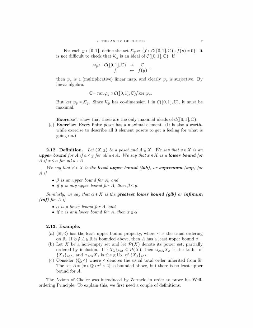
For each y ∈ [0,1], define the set Ky ∶= f ∈ C([0,1],C) ∶ f(y) = 0. Itis not difficult to check that Ky is an ideal of C([0,1],C). If

ϕy ∶ C([0,1],C) → Cf ↦ f(y)

,

then ϕy is a (multiplicative) linear map, and clearly ϕy is surjective. Bylinear algebra,

C = ranϕy ≃ C([0,1],C)/ker ϕy.

But ker ϕy = Ky. Since Ky has co-dimension 1 in C([0,1],C), it must bemaximal.

Exercise∗: show that these are the only maximal ideals of C([0,1],C).(e) Exercise: Every finite poset has a maximal element. (It is also a worth-

while exercise to describe all 3 element posets to get a feeling for what isgoing on.)

2.12. Definition. Let (X,≤) be a poset and A ⊆ X. We say that y ∈ X is anupper bound for A if a ≤ y for all a ∈ A. We say that x ∈X is a lower bound forA if x ≤ a for all a ∈ A.

We say that β ∈ X is the least upper bound (lub), or supremum (sup) forA if

β is an upper bound for A, and if y is any upper bound for A, then β ≤ y.

Similarly, we say that α ∈ X is the greatest lower bound (glb) or infimum(inf) for A if

α is a lower bound for A, and if x is any lower bound for A, then x ≤ α.

2.13. Example.

(a) (R,≤) has the least upper bound property, where ≤ is the usual orderingon R. If ∅ /= A ⊆ R is bounded above, then A has a least upper bound β.

(b) Let X be a non-empty set and let P(X) denote its power set, partiallyordered by inclusion. If Xλλ∈Λ ⊆ P(X), then ∪λ∈ΛXλ is the l.u.b. ofXλλ∈Λ, and ∩λ∈ΛXλ is the g.l.b. of Xλλ∈Λ.

(c) Consider (Q,≤) where ≤ denotes the usual total order inherited from R.The set A = x ∈ Q ∶ x2 < 2 is bounded above, but there is no least upperbound for A.

The Axiom of Choice was introduced by Zermelo in order to prove his Well-ordering Principle. To explain this, we first need a couple of definitions.


2.14. Definition. A non-empty poset (X,≤) is said to be well-ordered ifevery non-empty subset A ⊆X has a mimimum element.

It immediately follows that every well-ordered set is totally ordered.

2.15. Example.

(a) The set N is well-ordered with the usual ordering, whereas R is not.(b) Let ω + 7 = 1,2,3, ...., ω, ω + 1, ω + 2, ..., ω + 6. Define a partial order on

ω + 7 by setting n ≤ ω + k for all n ≥ 1, 0 ≤ k ≤ 6 and ω + i ≤ ω + j if0 ≤ i ≤ j ≤ 6. The ordering on N ⊆ ω + 7 is the usual ordering on N. Thenω + 7 is well-ordered.

2.16. Theorem. The following are equivalent:

(i) The Axiom of Choice (AC): given a non-empty collection Xλλ∈Λ of non-empty sets, ∏λ∈ΛXλ /= ∅.

(ii) Zorn’s Lemma (ZL): Let (Y,≤) be a poset. Suppose that every chain C ⊆ Yhas an upper bound. Then Y has a maximal element.

(iii) The Well-Ordering Principle (WO): Every non-empty set Z admits a well-ordering.

Proof. This result has been moved to PM433. You may consult the appendix tothis Chapter for a proof.

◻

2.17. Theorem. Every vector space V has a basis.Proof. See Assignment One.

◻

2.18. Many results are known to be equivalent to the Axiom of Choice (inZermelo-Frankel theory). In fact, the above result from Theorem 2.17 is amongstthese.

Others include:

Let V be a vector space over a field F and suppose that J ⊆ S ⊆ V , whereJ is a linearly independent subset of V , and spanS = V . Then there existsa basis B for V with J ⊆ B ⊆ S.

If X and Y /= ∅ are disjoint sets and X is infinite, then there exists abijection between X × Y and X ∪ Y .

If a set A is infinite, then there is a bijection between the sets A and A×A. Given sets A and B, either there exists an injection from A into B, or there

exists an injection from B into A. Every unital ring R contains a maximal ideal. Let X be a set and F be a collection of subsets of X. Suppose that F

has finite character, that is: Y ∈ F if and only if each finite subset FYof Y lies in F . Then any member of F is a subset of some maximal (withrespect to containment) member of F .


The following results are known to be weaker than the Axiom of Choice. Theyare mentioned for information purposes at this point - some definitions will eventu-ally follow.

Any countable union of countable sets is countable. Every Hilbert space has an orthonormal basis. The Hahn-Banach Theorem.

Throughout this course we shall follow the standard usage of the Axiom ofChoice, namely: we shall assume that it holds, but we shall mention it explicitlywhenever it is used.

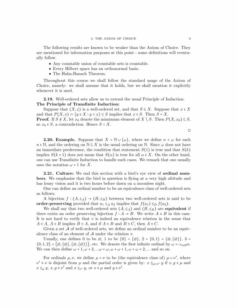
2.19. Well-ordered sets allow us to extend the usual Principle of Induction.The Principle of Transfinite Induction:

Suppose that (X,≤) is a well-ordered set, and that S ⊆ X. Suppose that x ∈ Xand that P (X,x) ∶= y ∈X ∶ y < x ⊆ S implies that x ∈ S. Then S =X.Proof. If S /=X, let x0 denote the mimimum element of X / S. Then P (X,x0) ⊆ S,so x0 ∈ S, a contradiction. Hence S =X.

◻

2.20. Example. Suppose that X = N ∪ ω, where we define n < ω for eachn ∈ N, and the ordering on N ⊆X is the usual ordering on N. Since ω does not havean immediate predecessor, the condition that statement S(1) is true and that S(k)implies S(k + 1) does not mean that S(α) is true for all α ∈X. On the other hand,one can use Transfinite Induction to handle such cases. We remark that one usuallyuses the notation ω + 1 for X.

2.21. Culture: We end this section with a bird’s eye view of ordinal num-bers. We emphasize that the bird in question is flying at a very high altitude andhas lousy vision and it is two hours before dawn on a moonless night.

One can define an ordinal number to be an equivalence class of well-ordered setsas follows.

A bijection f ∶ (A,≤A) → (B,≤B) between two well-ordered sets is said to beorder-preserving provided that a1 ≤A a2 implies that f(a1) ≤B f(a2).

We shall say that two well-ordered sets (A,≤A) and (B,≤B) are equivalent ifthere exists an order preserving bijection f ∶ A → B. We write A ≡ B in this case.It is not hard to verify that ≡ is indeed an equivalence relation in the sense thatA ≡ A, A ≡ B implies B ≡ A, and if A ≡ B and B ≡ C, then A ≡ C.

Given a set A of well-ordered sets, we define an ordinal number to be an equiv-alence class of an element of A under the relation ≡.

Usually, one defines 0 to be ∅, 1 to be 0 = ∅, 2 = 0,1 = ∅,∅, 3 =

0,1,2 = ∅,∅,∅,∅, etc. We denote the first infinite ordinal by ω = ∪n≥0n.We can then define ω + 1, ω + 2, ...ω + ω,ω + ω + 1, ω + ω + 2, ... and so on.

For ordinals µ, ν, we define µ + ν to be (the equivalence class of) µ ∪ ν′, whereν′ ≡ ν is disjoint from µ and the partial order is given by: x ≤µ+ν′ y if x, y ∈ µ andx ≤µ y, x, y ∈ ν′ and x ≤ν′ y, or x ∈ µ and y ∈ ν′.


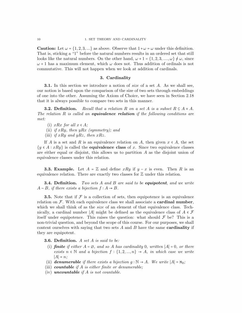
Caution: Let ω = 1,2,3, ... as above. Observe that 1+ω = ω under this definition.That is, sticking a “1” before the natural numbers results in an ordered set that stilllooks like the natural numbers. On the other hand, ω + 1 = 1,2,3, ...., ω /= ω, sinceω + 1 has a maximum element, which ω does not. Thus addition of ordinals is notcommutative. This will not happen when we look at addition of cardinals.

3. Cardinality

3.1. In this section we introduce a notion of size of a set A. As we shall see,our notion is based upon the comparison of the size of two sets through embeddingsof one into the other. Assuming the Axiom of Choice, we have seen in Section 2.18that it is always possible to compare two sets in this manner.

3.2. Definition. Recall that a relation R on a set A is a subset R ⊆ A × A.The relation R is called an equivalence relation if the following conditions aremet:

(i) xRx for all x ∈ A;(ii) if xRy, then yRx (symmetry); and(iii) if xRy and yRz, then xRz.

If A is a set and R is an equivalence relation on A, then given x ∈ A, the sety ∈ A ∶ xRy is called the equivalence class of x. Since two equivalence classesare either equal or disjoint, this allows us to partition A as the disjoint union ofequivalence classes under this relation.

3.3. Example. Let A = Z and define xRy if y − x is even. Then R is anequivalence relation. There are exactly two classes for Z under this relation.

3.4. Definition. Two sets A and B are said to be equipotent, and we writeA ∼ B, if there exists a bijection f ∶ A→ B.

3.5. Note that if F is a collection of sets, then equipotence is an equivalencerelation on F . With each equivalence class we shall associate a cardinal number,which we shall think of as the size of an element of that equivalence class. Tech-nically, a cardinal number ∣A∣ might be defined as the equivalence class of A ∈ F

itself under equipotence. This raises the question: what should F be? This is anon-trivial question, and beyond the scope of this course. For our purposes, we shallcontent ourselves with saying that two sets A and B have the same cardinality ifthey are equipotent.

3.6. Definition. A set A is said to be:

(i) finite if either A = ∅, and so A has cardinality 0, written ∣A∣ = 0, or thereexists n ∈ N and a bijection f ∶ 1,2, ..., n → A, in which case we write∣A∣ = n;

(ii) denumerable if there exists a bijection g ∶ N→ A. We write ∣A∣ = ℵ0;(iii) countable if A is either finite or denumerable;(iv) uncountable if A is not countable.

3. CARDINALITY 11

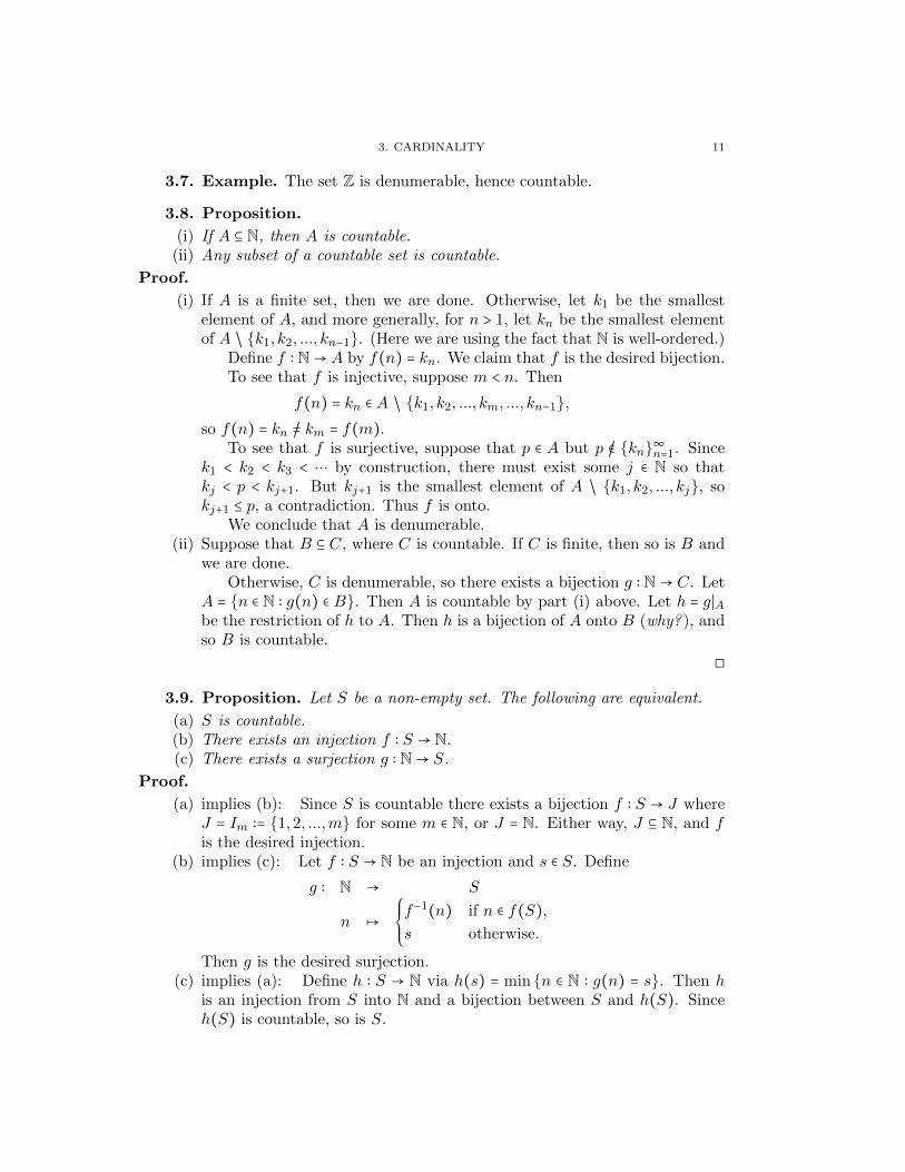
3.7. Example. The set Z is denumerable, hence countable.

3.8. Proposition.

(i) If A ⊆ N, then A is countable.(ii) Any subset of a countable set is countable.

Proof.

(i) If A is a finite set, then we are done. Otherwise, let k1 be the smallestelement of A, and more generally, for n > 1, let kn be the smallest elementof A / k1, k2, ..., kn−1. (Here we are using the fact that N is well-ordered.)

Define f ∶ N→ A by f(n) = kn. We claim that f is the desired bijection.To see that f is injective, suppose m < n. Then

f(n) = kn ∈ A / k1, k2, ..., km, ..., kn−1,

so f(n) = kn /= km = f(m).To see that f is surjective, suppose that p ∈ A but p /∈ kn

∞n=1. Since

k1 < k2 < k3 < ⋯ by construction, there must exist some j ∈ N so thatkj < p < kj+1. But kj+1 is the smallest element of A / k1, k2, ..., kj, sokj+1 ≤ p, a contradiction. Thus f is onto.

We conclude that A is denumerable.(ii) Suppose that B ⊆ C, where C is countable. If C is finite, then so is B and

we are done.Otherwise, C is denumerable, so there exists a bijection g ∶ N→ C. Let

A = n ∈ N ∶ g(n) ∈ B. Then A is countable by part (i) above. Let h = g∣Abe the restriction of h to A. Then h is a bijection of A onto B (why? ), andso B is countable.

◻

3.9. Proposition. Let S be a non-empty set. The following are equivalent.

(a) S is countable.(b) There exists an injection f ∶ S → N.(c) There exists a surjection g ∶ N→ S.

Proof.

(a) implies (b): Since S is countable there exists a bijection f ∶ S → J whereJ = Im ∶= 1,2, ...,m for some m ∈ N, or J = N. Either way, J ⊆ N, and fis the desired injection.

(b) implies (c): Let f ∶ S → N be an injection and s ∈ S. Define

g ∶ N → S

n ↦

⎧⎪⎪⎨⎪⎪⎩

f−1(n) if n ∈ f(S),

s otherwise.

Then g is the desired surjection.(c) implies (a): Define h ∶ S → N via h(s) = minn ∈ N ∶ g(n) = s. Then h

is an injection from S into N and a bijection between S and h(S). Sinceh(S) is countable, so is S.


◻

3.10. Example.

(a) Recall that every natural number has a unique factorization as a productof primes (up to the order of the factors). Suppose that A and B arenon-empty countable sets. We claim that the Cartesian product A ×B iscountable.

Let f ∶ A→ N and g ∶ B → N be injections. Define

h ∶ A ×B → N(a, b) ↦ 2f(a)3g(b).

It is routine to verify that h is injective, and hence that A×B is count-able.

(b) Suppose that An∞n=1 is a collection of denumerable sets. Then A = ∪n≥1An

is denumerable.We shall prove this in the case where An∩Am = ∅ if n /=m. The general

case follows easily from this (exercise). Since An is denumerable, we canwrite An = an1, an2, an3, ... for each n ≥ 1. Construct a new sequence via:

Then A = a11, a12, a21, a31, a22, a13, a14, .... Thus A is countable.(c) The set Q of rational numbers is countable. Indeed, for each n ≥ 1, let

An = 0/n,1/n,−1/n,2/n,−2/n,3/n,−3/n, .... Then Q = ∪n≥1An. By (b)above, Q is countable.

Recall that between any two distinct rational numbers there are infinitely manyrational numbers, and that between any two distinct irrational numbers one canfind infinitely many rational numbers. One might be tempted to believe that theset I of irrational numbers and the set Q of rational numbers are equipotent. Thatwould be a mistake.

3.11. Theorem. The set R of real numbers is uncountable.Proof. Using Cantor’s diagonal process, we shall prove that (0,1) is uncountable.By Proposition 3.8, this implies that R is uncountable.

If (0,1) were countable, then we could write (0,1) = xn∞n=1, where

3. CARDINALITY 13

x1 = 0.x11 x12 x13 x14...

x2 = 0.x21 x22 x23 x24...

x3 = 0.x31 x32 x33 x34...

x4 = 0.x41 x42 x43 x44...

⋮

in decimal form, so that xij is an integer between 0 and 9.Let y = 0.y1 y2 y3 y4... where yn = 7 if xnn ∈ 0,1,2,3,4,5 and yn = 3 if

xnn ∈ 6,7,8,9. Then y /= xn, since yn /= xnn for all n ≥ 1.In other words, y ∈ (0,1), but y /∈ xn

∞n=1, a contradiction.

◻

3.12. Although N ⊂ Z ⊂ Q, all three sets are equipotent, and we write ∣N∣ = ∣Z∣ =

∣Q∣ = ℵ0. Thus it is not enough for one set to properly contain another in order tohave greater cardinality (although this does work for finite sets). Nevertheless, ourintuition tells us that if f ∶ A→ B is an injection, then we would expect A to be nolarger than B.

Letting ∣A∣ denote the cardinality of A, we shall define ∣A∣ ≤ ∣B∣ to mean thatthere exists an injection f ∶ A → B. Then ∣A∣ < ∣B∣ means that ∣A∣ ≤ ∣B∣, but that∣A∣ /= ∣B∣. That is, although an injection f ∶ A → B exists, there is no bijectiong ∶ A→ B. This agrees with the usual notion of size when the sets are finite.

3.13. Theorem. Let A,B, and C be sets.

(i) If A ⊆ B, then ∣A∣ ≤ ∣B∣.(ii) ∣A∣ ≤ ∣A∣.(iii) If ∣A∣ ≤ ∣B∣ and ∣B∣ ≤ ∣C ∣, then ∣A∣ ≤ ∣C ∣.(iv) If m,n ∈ N and m ≤ n, then ∣1,2, ...,m∣ ≤ ∣1,2, ..., n∣.(v) If E is finite, then ∣E∣ < ℵ0.

Proof. Exercise.

◻

3.14. Let us denote ∣R∣ by c (for continuum). Since N ⊆ R, ℵ0 ≤ c. In fact, sinceR is uncountable, ℵ0 < c. That is, there are at least two infinite cardinals. In fact,there are many, many more.

3.15. Theorem. For any set X, ∣X ∣ < ∣P(X)∣, where P(X) is the power set ofX.Proof. First note that the map

f ∶ X → P(X)

x ↦ x

is injective, and so ∣X ∣ ≤ ∣P(X)∣.


Next, suppose that g ∶ X → P(X) is any surjective map. Given x ∈ X, eitherx ∈ g(x), or x /∈ g(x). Let T = x ∈ X ∶ x /∈ g(x). Since g is surjective, there existsz ∈X so that g(z) = T .

If z ∈ T , then z ∈ g(z), so z /∈ T , a contradiction.If z /∈ T , then z /∈ g(z), so z ∈ T , again a contradiction.Thus g can not be surjective, and a fortiori it can not be bijective, so ∣X ∣ <

∣P(X)∣.

◻

3.16. It follows that ℵ0 = ∣N∣ < ∣P(N)∣ < ∣P(P(N))∣ < ∣P(P(P(N)))∣ < ⋯, andthat there exist infinitely many infinite cardinal numbers. Where does c = ∣R∣ fit?We have seen that ℵ0 < c, but does there exist an infinite cardinal λ such thatℵ0 < λ < c? Writing ℵ1 for the first cardinal bigger than ℵ0, the question becomes:is c = ℵ1?

The conjecture that there does not exist such a λ is known as the ContinuumHypothesis and is due to Georg Cantor. In 1938, Kurt Godel proved that theContinuum Hypothesis does not contradict the usual axioms of set theory. In 1963,Paul Cohen prove that the negation of the Continuum Hypothesis is also consistentwith the usual axioms of set theory.

Whereas the Axiom of Choice is freely used (but cited) by the majority ofmathematicians, it is not standard to assume the Continuum Hypothesis nor itsnegation. In the few instances where it is used, it must be explicitly stated that oneis using it. If it is possible to prove something without assuming the ContinuumHypothesis, then it is generally considered best to prove it without using it.

4. Cardinal Arithmetic

4.1. In this section we shall briefly examine sums, products and powers of car-dinal numbers. Finite numbers do not provide the best intuition, since we don’texpect numbers other than 1 to satisfy λ2 = λ, for example. This equality will besatisfied by infinite cardinals, as we shall soon see. We begin with an extremely use-ful result which is the usual tool for proving that two sets have the same cardinality.Although the result looks obvious, its proof is surprisingly non-obvious.

4.2. Theorem. The Schroder-Bernstein Theorem. Let A and B be sets.If ∣A∣ ≤ ∣B∣ and ∣B∣ ≤ ∣A∣, then ∣A∣ = ∣B∣.Proof. Step One: If Z is any set and ϕ ∶ P(Z) → P(Z) is increasing in thesense that X ⊆ Y ⊆ Z implies that ϕ(X) ⊆ ϕ(Y ), then ϕ has a fixed point; that is,there exists T ⊆X such that ϕ(T ) = T .

Indeed, let T = ∪X ⊆ Z ∶X ⊆ ϕ(X). If X ⊆ Z and X ⊆ ϕ(X), then X ⊆ T andso ϕ(X) ⊆ ϕ(T ). That is, X ⊆ Z and X ⊆ ϕ(X) implies X ⊆ ϕ(T ), and thus

T = ∪X ⊆ Z ∶X ⊆ ϕ(X) ⊆ ϕ(T ).

4. CARDINAL ARITHMETIC 15

But then ϕ(T ) ⊆ Z and ϕ(T ) ⊆ ϕ(ϕ(T )), so that ϕ(T ) is one of the sets appearingin the definition of T - i.e. ϕ(T ) ⊆ T .

Together, these imply that ϕ(T ) = T . (We remark that it is entirely possiblethat T = ∅.)

Step Two: Given sets A,B as above and injections κ ∶ A → B and λ ∶ B → A,define

ϕ ∶ P(A) → P(A)

X ↦ A / λ[B / κ(X)].

Suppose X ⊆ Y ⊆ A. Then κ(X) ⊆ κ(Y ).Hence

B / κ(X) ⊇ B / κ(Y ), so

λ(B / κ(X)) ⊇ λ(B / κ(Y )), which implies

A / λ(B / κ(X)) ⊆ A / λ(B / κ(Y )), which in turn implies

ϕ(X) ⊆ ϕ(Y ).

Step Three: By Steps One and Two, there exists T ⊆ A such that T = ϕ(T ) =

A / λ[B / κ(T )].Define

f ∶ A → B

a ↦

⎧⎪⎪⎨⎪⎪⎩

κ(a) if a ∈ T ,

λ−1(a) if a ∈ A / T .

Observe that λ is a bijection between B / κ(T ) and A / T , and that κ is abijection between T and κ(T ), so that f is a bijection between A and B.

◻

Using the Schroder-Bernstein Theorem, we can prove the following:

4.3. Theorem. c = ∣R∣ = ∣P(N)∣.Proof. By the Schroder-Bernstein Theorem, it suffices to prove that c ≤ ∣P(N)∣ and∣P(N)∣ ≤ c.

To see that ∣P(N)∣ ≤ c, define

f ∶ P(N) → RA ↦ 0.a1 a2 a3 ...

where an = 0 if n /∈ A and an = 1 if n ∈ A. It is not hard to verify that f is injective.To see that c ≤ ∣P(N)∣, first note that ∣N∣ = ∣Q∣ and hence (exercise) ∣P(N)∣ =

∣P(Q)∣. Next, let

g ∶ R → P(Q)

x ↦ y ∈ Q ∶ y < x.

If x1 < x2 in R, then there exists q ∈ Q so that x1 < q < x2, and so q /∈ g(x1) butq ∈ g(x2), showing that g(x1) /= g(x2) and so g is injective.

◻


4.4. Definition. Let α,β be cardinal numbers.The sum α + β of α and β is defined to be the cardinal ∣A ∪B∣, where A and B

are disjoint sets such that ∣A∣ = α and ∣B∣ = β.

The product α β of α and β is the cardinal number ∣A×B∣, where A and B aresets with ∣A∣ = α and ∣B∣ = β.

The power βα is defined as ∣BA∣, where A and B are sets with ∣A∣ = α and∣B∣ = β.

4.5. In “ordinal arithmetic”, one defines 0 = ∅, 1 = 0 = ∅, 2 = 0,1 =

∅,∅, 3 = 0,1,2, etc. In a mild abuse of notation, the same notation is usedto denote the corresponding cardinal.

The proof of Theorem 4.3 shows that if A is any set and B is a subset of A,then B corresponds to a unique function fB ∶ A→ 0,1 given by fB(a) = 0 if a /∈ B,and fB(a) = 1 if a ∈ B. (This is often called the characteristic function or theindicator function of B in A.)

The map B ↦ fB is a bijection between P(A) and 0,1A = 2A. Thus ∣P(A)∣ =

∣2A∣, and in particular, ∣2N∣ = ∣P(N)∣ = c. But, from the definition of cardinal powers,

this says that c = ∣2N∣ = ∣2∣∣N∣ = 2ℵ0 .

4.6. Lemma.

(i) If A is an infinite set, then A contains a denumerable subset.(ii) If A is an infinite set and B is a finite set, then ∣A∣ + ∣B∣ = ∣A∣.

Proof.

(i) Since A /= ∅, there exists x1 ∈ A. Then A / x1 /= ∅, otherwise A would befinite.

In general, for n ≥ 1, having chosen x1, x2, ..., xn ⊆ A, we know thatA / x1, x2, ..., xn /= ∅, so we can find xn+1 ∈ A / x1, x2, ..., xn. (Doingthis for all n ≥ 1 requires the Axiom of Choice - or at least a weak versionof it.)

The function f ∶ N → A defined via f(n) = xn is an injection, and it isa bijection between N and B = ran f = xn

∞n=1. Thus ∣B∣ = ℵ0 and B is a

denumerable subset of A.(ii) Let A be an infinite set, and let D ⊆ A be a denumerable subset of A.

Suppose that B = b1, b2, ..., bn. (We may suppose that B∩A = ∅ (why? )).Define a map

f ∶ A ∪B → Az ↦ z if z ∈ A / Dbi ↦ di if 1 ≤ i ≤ n,dk ↦ dk+n, for all k ≥ 1.

Then f is an bijection of A ∪B onto A, and so ∣A∣ + ∣B∣ = ∣A∣.

◻


4.7. Theorem. Let α,β, and γ be cardinal numbers. Then

(i) α + β is well-defined. That is, if ∣A∣ = ∣C ∣, ∣B∣ = ∣D∣ and A ∩B = ∅ = C ∩D,then ∣A ∪B∣ = ∣C ∪D∣.

(ii) α + β = β + α and (α + β) + γ = α + (β + γ).(iii) If β is infinite and α ≤ β, then α + β = β.

Proof.

(i) Exercise.(ii) Exercise.(iii) The case where α < ℵ0 is Lemma 4.6.

First let us show that β + β = β. Choose a set B with ∣B∣ = β. ThenB × 2 = (B × 0) ∪ (B × 1) is the union of two disjoint sets equipotentwith B, so it suffices to show that ∣B × 2∣ = ∣B∣ = β.

Let F = (X,f) ∶ X ⊆ B and f ∶ X → X × 2 is a bijection, partiallyordered by (X1, f1) ≤ (X2, f2) if X1 ⊆X2 and f2∣X1 = f1.

If X ⊆ B is denumerable, then ∣X × 2∣ = ∣X ∣ = ℵ0 by Example 3.10, andhence F /= ∅.

Suppose that C = (Xα, fα)α∈Λ is a chain in F .Let X = ∪α∈ΛXα. For x ∈ X, choose α ∈ Λ such that x ∈ Xα. Define

f(x) = fα(x). Then f is well-defined (why? ). Moreover, (X,f) is an upperbound for C; i.e. f ∶X →X × 2 is a bijection (exercise).

By Zorn’s Lemma, F has a maximal element (Y, g). We claim thatB / Y is finite. Otherwise, choose a denumerable set Z ⊆ B / Y . Since∣Z ∣ = ∣Z × 2∣ = ℵ0, there exists a bijection h ∶ Z → Z × 2. Define a bijection

h ∶ Y ∪Z → (Y ∪Z) × 2

w ↦

⎧⎪⎪⎨⎪⎪⎩

g(w) if w ∈ Y ,

h(w) if w ∈ Z.

Then (Y ∪Z,h) > (Y, g), contradicting the maximality of (Y, g).This shows that B / Y is finite. Hence ∣Y ∣ = ∣B∣ = β, and so β = ∣Y ∣ =

∣Y × 2∣ = ∣Y ∣ + ∣Y ∣ = β + β.Finally, in general we have β ≤ α + β ≤ β + β = β, so that by the

Schroder-Bernstein Theorem, α + β = β.

◻

4.8. Theorem. Let α,β, γ, δ be cardinal numbers. Then

(i) α ⋅ β is well-defined. That is, if ∣A∣ = ∣C ∣, ∣B∣ = ∣D∣, then ∣A ×B∣ = ∣C ×D∣.(ii) α ⋅ β = β ⋅ α; α(β ⋅ γ) = (α ⋅ β)γ; and α(β + γ) = α ⋅ β + α ⋅ γ.(iii) 0 ⋅ α = 0.(iv) If α ≤ β and γ ≤ δ, then α ⋅ γ ≤ β ⋅ δ.(v) α ⋅ α = α if α is infinite.

Proof.

(i) Exercise.(ii) Exercise.


(iii) Exercise.(iv) Exercise.(v) Suppose that ∣A∣ = α. Let F = (X,f) ∶X ⊆ A,f ∶X →X×X is a bijection,

partially ordered by (X1, f1) ≤ (X2, f2) if X1 ⊆X2 and f2∣X1 = f1.Since A is infinite, it contains a denumerable set X. Now by Exam-

ple 3.10, if X ⊆ A is denumerable, then there exists a function f so that(X,f) ∈ F , and thus F /= ∅. By Zorn’s Lemma (as before), there exists amaximal element (Y, g) in F .

Then ∣Y ∣ ⋅ ∣Y ∣ = ∣Y ∣, so it suffices to show that ∣Y ∣ = α.Assume that ∣Y ∣ < α. Since α = ∣Y ∣+ ∣A / Y ∣, it follows that ∣A / Y ∣ = α,

and so ∣Y ∣ < ∣A / Y ∣. Thus A / Y has a subset Z with ∣Z ∣ = ∣Y ∣. ThenY × Z,Z × Y and Z × Z are disjoint, infinite sets with cardinality ∣Y ∣, andso

∣(Y ×Z) ∪ (Z × Y ) ∪ (Z ×Z)∣ = ∣Y ×Z ∣ + ∣Z × Y ∣ + ∣Z ×Z ∣

= (∣Y ∣ ⋅ ∣Y ∣) + (∣Y ∣ ⋅ ∣Y ∣) + (∣Y ∣ ⋅ ∣Y ∣)

= ∣Y ∣ + ∣Y ∣ + ∣Y ∣

= ∣Y ∣

= ∣Z ∣.

Thus there exists a bijection h ∶ Z → (Y ×Z) ∪ (Z × Y ) ∪ (Z ×Z).Define the map

m ∶ Y ∪Z → (Y ∪Z) × (Y ∪Z)

x ↦

⎧⎪⎪⎨⎪⎪⎩

g(x) if x ∈ Y

h(x) if x ∈ Z

.

Then m is a bijection and so (Y ∪ Z,m) ∈ F with (Y, g) < (Y ∪ Z,m),contradicting the maximality of (Y, g) in F .

This contradiction shows that ∣Y ∣ = α, and we are done, as g ∶ Y → Y ×Yis the bijection which implies that α = α ⋅ α.

◻

4.9. Theorem. Let α,β and γ be cardinal numbers. Then

(i) αβ is well-defined. That is, if A1,A2,B1,B2 are sets with ∣A1∣ = α = ∣A2∣

and ∣B1∣ = β = ∣B2∣, then ∣AB11 ∣ = ∣AB2

2 ∣.

(ii) (αβ)γ = α(βγ).

(iii) α(β+γ) = αβ αγ.

Proof.

(i) Exercise.(ii) Let A,B and C be sets with ∣A∣ = α, ∣B∣ = β and ∣C ∣ = γ. We must show

that ∣(AB)C ∣ = ∣AB×C ∣.Now if f ∈ AB×C , then for each c ∈ C, the function fc given by fc(b) ∶=

f(b, c) defines an element of AB. Define ϕf ∶ C → AB by ϕf(c) = fc. Then


the correspondence

Φ ∶ AB×C → (AB)C

f ↦ ϕf

is a bijection. Indeed, if Φ(f) = Φ(g) for f, g ∈ AB×C , then ϕf = ϕg, and sofor every c ∈ C, fc = ϕf(c) = ϕg(c) = gc. But fc = gc for all c ∈ C impliesthat f(b, c) = fc(b) = gc(b) = g(b, c) for all b ∈ B and for all c ∈ C, so thatf = g. This shows that Φ is injective.

Given τ ∈ (AB)C , we see that τ(c) ∈ AB for all c ∈ C, and so we definef ∶ B × C → A via f(b, c) = [τ(c)](b). It is clear that f ∈ AB×C and thatΦ(f) = τ , so that Φ is onto. Finally, since Φ is a bijection, ∣AB×C ∣ = ∣(AB)C ∣,completing the proof.

(iii) Now suppose that B ∩C = ∅. We must show that ∣AB∪C ∣ = ∣AB ×AC ∣. Butevery f ∶ B ∪ C → A is defined by its restrictions to B and C, so we aredone.

◻

4.10. Example.

(a) ℵ0 + ℵ0 = ℵ0.(b) ℵ0 + c = c.(c) c ⋅ c = c.

(d) cℵ0 = (2ℵ0)ℵ0 = 2(ℵ0⋅ℵ0) = 2ℵ0 = c.


5. Appendix

In this Appendix we shall provide a proof of the equivalence of the Axiomof Choice, Zorn’s Lemma and the Well-Ordering Principle. We begin with thedefinition of an initial segment, which will be required in the proof.

5.1. Definition. Let (X,≤) be a poset, C ⊆ X be a chain in X and d ∈ C. Wedefine

P (C,d) = c ∈ C ∶ c < d.

An initial segment of C is a subset of the form P (C,d) for some d ∈ C.

5.2. Example.

(a) For each r ∈ R, (−∞, r) is an initial segment of (R,≤).(b) For each n ∈ N, 1,2, ..., n is an initial segment of N.

5.3. Theorem. The following are equivalent:

(i) The Axiom of Choice (AC): given a non-empty collection Xλλ∈Λ of non-empty sets, ∏λ∈ΛXλ /= ∅.

(ii) Zorn’s Lemma (ZL): Let (Y,≤) be a poset. Suppose that every chain C ⊆ Yhas an upper bound. Then Y has a maximal element.

(iii) The Well-Ordering Principle (WO): Every non-empty set Z admits a well-ordering.

Proof.

(i) implies (ii): This is the most delicate of the three implications. We shallargue by contradiction.

Suppose that (X,≤) is a poset such that every chain in X is boundedabove, but that X no maximal elements. Given a chain C ⊆ X, we canfind an upper bound uC for C. Since uC is not a maximal element, we canfind vC ∈X with uC < vC . We shall refer to such an element vC as a strictupper bound for C.

By the Axiom of Choice, for each chain C in X, we can choose a strictupper bound f(C). If C = ∅, we arbitrarily select x0 ∈X and set f(∅) = x0.

We shall say that a subset A ⊆X satisfies property L if(I) The partial order ≤ on X when restricted to A is a well-ordering of A,

and(II) for all x ∈ A, x = f(P (A,x)). Claim 1: if A,B ⊆ X satisfy property L and A /= B, then either A is aninitial segment of B, or B is an initial segment of A.

Without loss of generality, we may assume that A / B /= ∅. Let

x = mina ∈ A ∶ a /∈ B.

5. APPENDIX 21

Note that x exists because A is well-ordered. Then P (A,x) ⊆ B. We shallargue that B = P (A,x). If not, then B / P (A,x) /= ∅, and using thewell-orderedness of B,

y = minb ∈ B ∶ b /∈ P (A,x)

exists. Thus P (B,y) ⊆ P (A,x).

Let z = min (A / P (B,y)). Then z ≤ x = min (A / B).

Subclaim 1: P (A, z) = P (B,y).By definition, P (A, z) ⊆ P (B,y).To obtain the reverse inclusion, we first argue that if t ∈ P (B,y) =

A∩P (B,y), then P (A, t)∪ t ⊆ P (B,y). By hypothesis, t ∈ P (B,y),so suppose that u ∈ P (A, t). Now t ∈ P (B,y) ⊆ P (A,x), so u < t < ximplies that u ∈ P (A,x). In other words, P (A, t) ⊆ P (A,x) ⊆ B. Butthen u ∈ B and u < t < y implies that u ∈ P (B,y).We now have that if s ∈ P (B,y), then P (A, s) ∪ s ⊆ P (B,y) ⊆

P (A,x) ⊆ A. This forces s < z ∶= min (A /P (B,y)), so that s ∈

P (A, z).Together, we find that P (B,y) ⊆ P (A, z) ⊆ P (B,y), which proves thesubclaim.

Returning to the proof of the claim, we now have that z = f(P (A, z)) =f(P (B,y)) = y. But y ∈ B, so y /= x. Hence z < x. Thus y = z ∈ P (A,x),contradicting the definition of y. We deduce that P (A,x) = B, and hencethat B is an initial segment of A, thereby proving our claim.

Suppose that A ⊆X has property L, and let x ∈ A. It follows from theabove argument that given y < x, either y ∈ A or y does not belong to anyset B with property L.

Let V = ∪A ⊆X ∶ A has property L.

Claim 2: We claim that if w = f(V ), then V ∪ w has property L.Suppose that we can show this. Then V ∪ w ⊆ V , so w ∈ V , a

contradiction. This will complete the proof.

Subclaim 2a: First we show that V itself has property L. We must showthat V is well-ordered, and that for all x ∈ V , x = f(P (V,x)).

(a) V is well-ordered.Let ∅ /= B ⊆ V . Then there exists A0 ⊆ X so that A0 has propertyL and B ∩ A0 /= ∅. Since A0 is well-ordered and ∅ /= B ∩ A0 ⊆ A0,m ∶= min(B ∩A0) exists. We claim that m = min(B).Suppose that y ∈ B. Then there exists A1 ⊆X so that A1 has propertyL and y ∈ A1. Now, both A0 and A1 have property L:

if A0 = A1, then m = min(B ∩A1), so m ≤ y. if A0 /= A1, then either


A0 is an initial segment of A1, so A0 = P (A1, d) for somed ∈ A1. Then

m = min(B ∩A0) = min(B ∩A1),

since r ∈ A1 ∖A0 implies that m < d ≤ r. Hence m ≤ y;, or A1 is an initial segment of A0, say A1 = P (A0, d) ⊆ A0 for

some d ∈ A0. Then

m = min(B ∩A0) ≤ min(B ∩A1).

Hence m ≤ y.In both cases we see that m ≤ y. Since y ∈ B was arbitrary, m =

min(B).Thus, any non-empty subset B of V has a minimum element, and soV is well-ordered.

(b) Let x ∈ V . Then there exists A2 ⊆ X with property L so that x ∈ A2.Then x = P (A2, x). Suppose that y ∈ V and y < x. Then there existsA3 ⊆ X with property L so that y ∈ A3. Since A2 and A3 both haveproperty L, either

A2 = A3, and so y ∈ A2; or A2 = P (A3, d) for some d ∈ A3. Since x ∈ A2, P (A2, x) =

P (A3, x) and therefore y ∈ A2; or A3 = P (A2, d) for some d ∈ A2. Then y ∈ A3 implies that y ∈ A2.

In any of these three cases, y ∈ A2. Hence P (V,x) ⊆ P (A2, x). SinceA2 ⊆ V , we have that P (A2, x) ⊆ P (V,x), whence P (A2, x) = P (V,x).But then

x = f(P (A2, x)) = f(P (V,x)).

By (a) and (b), V has property L.

We now return to the proof of Claim 2. That is, we prove that ifw = f(V ), then V ∪ w has property L.

(I) V ∪ w is well-ordered.We know that V is well-ordered by part (a) above. Suppose that ∅ /=

B ⊆ V ∪ w. If B ∩V /= ∅, then by (a) above, m ∶= min(B ∩V ) exists.Clearly m ∈ V implies m ≤ f(V ) = w, so m = min(B ∩ (V ∪ w)).If ∅ /= B ⊆ V ∪ w and B ∩ V = ∅, then B = w, and so w = min(B)

exists.Hence V ∪ w is well-ordered.

(II) Let x = V ∪ w. If x ∈ V , then x = f(P (V,x)) by part (a). If x = w,then

P (V ∪ w, x) = P (V ∪ w,w) = V,

so x = w = f(V ) = f(P (V ∪ w, x)).By (I) and (II), V ∪ w has property L. As we saw in the statement fol-lowing Claim 2, this completes the proof that the Axiom of Choice impliesZorn’s Lemma. Now let us never speak of this again.

5. APPENDIX 23

(ii) implies (iii): Let X /= ∅ be a set. It is clear that every finite subset F ⊆Xcan be well-ordered. Let A denote the collection of pairs (Y,≤Y ), whereY ⊆ X and ≤Y is a well-ordering of Y . For (A,≤A), (B,≤B) ∈ A, observethat A is an initial segment of B if the following two conditions are met: A ⊆ B and a1 ≤A a2 implies that a1 ≤B a2; if b ∈ B / A, then a ≤B b for all a ∈ A.Let us partially order A by setting (A,≤A) ≤ (B,≤B) if A is an initial

segment of B. Let C = Cλλ∈Λ be a chain in A.Then (exercise): ∪λ∈ΛCλ is an upper bound for C.By Zorn’s Lemma, A admits a maximal element, say (M,≤M). We

claim that M = X. Suppose otherwise. Then we can choose x0 ∈ X / Mand set M0 = M ∪ x0. define a partial order on M0 via: x ≤M0 y ifeither (a) x, y ∈ M and x ≤M y, or (b) x is arbitrary and y = x0. Then(M0,≤M0) is a well-ordered set and (M,≤M) < (M0,≤M0), a contradictionof the maximality of (M,≤M). Thus M = X and ≤M is a well- ordering ofX.

(iii) implies (i): Suppose that Xλλ∈Λ is a non-empty collection of non-emptysets. Let X = ∪λ∈ΛXλ. By hypothesis, X admits a well-ordering ≤X . Sinceeach ∅ /=Xλ ⊆X, it has a minimum element relative to the ordering on X.Define a choice function f by setting f(λ) to be this minimum element ofXλ for each λ ∈ Λ.

◻

We include a proof of an exercise mentioned earlier in the notes:

5.4. Proposition. The following are equivalent:

(a) The Axiom of choice: if Λ /= ∅ and for each λ ∈ Λ there exists a non-emptyset Xλ, then

Πλ∈ΛXλ /= ∅.

(b) If ∅ /= ∅, then there exists a function

g ∶ P(X) ∖ ∅→X

such that g(Y ) ∈ Y for all Y ⊆X.

Proof.

(a) implies (b).Suppose (a) holds. Let ∅ /= X be a set and set Λ = P(X) ∖ ∅. For

each Y ∈ Λ, set ZY = Y /= ∅.By the Axiom of Choice, there exists a choice function

f ∈ ΠY ∈ΛZY = ΠY ∈ΛY.

But then f(Y ) ∈ ZY = Y for each Y ∈ Λ = P(X) ∖ ∅.That is, (b) holds.

(b) implies (a).Suppose that (b) holds.


Let ∅ /= Λ be a set and suppose that Xλ is a non-empty set for eachλ ∈ Λ. Let Y = ∪λ∈ΛXλ.

By hypothesis, there exists a function g ∶ P(Y ) ∖ ∅ → Y so thatg(W ) ∈ W for all W ∈ P(Y ) ∖ ∅. In particular, each Xλ ∈ P(Y ) ∖ ∅,and so g(Xλ) ∈Xλ for all λ ∈ Λ.

Define f(λ) = g(Xλ), λ ∈ Λ. Then f is a choice function, so (a) holds.

◻

Culture.

(a) The basic axioms of set theory are referred to as the Zermelo-FrankelAxioms, or (ZF).

Godel proved that the Axiom of Choice is consistent with (ZF), but that(ZF) does not by itself imply the Axiom of Choice. Cohen then developedthe theory of “forcing” to prove that (ZF) plus the negation of the Axiomof Choice is also consistent.

(b) It is known that the Riemann hypothesis is true in (ZF) if and only if it istrue in (ZFC), namely (ZF) plus the Axiom of Choice.

(c) The generalized Continuum hypothesis (GCH) is known to be independentof (ZFC), however (ZF) plus (GCH) together imply the Axiom of Choice(AC).

(d) Tarski tried to publish the result which says that the Axiom of Choice (AC)is equivalent to the assertion that ∣A∣ = ∣A×A∣ whenever A is infinite in theComptes Rendus. It was not accepted. Frechet said that the equivalenceof two true statements is not something new, while Lebesgue said that anyimplication between two false propositions is of no interest.

CHAPTER 2

Metric spaces and normed linear spaces

1. An introduction

If you haven’t got anything nice to say about anybody, come sit nextto me.

Alice Roosevelt Longworth

1.1. In this Chapter we shall turn our attention to metric spaces. These aresets endowed with a well-behaved notion of distance. Notions such as limits andcontinuity extend naturally to this context. Our reasons for studying metric spacesare two-fold:

we prove general results once, rather than proving equivalent versions manytimes; and

by removing the non-essential properties of a specific metric space, we arriveat a better understanding of the underlying concept.

We pause briefly to introduce some notation. When we do not wish to specifyif we are using the real numbers R or the complex numbers C, we shall use K todenote the field.

1.2. Definition. A metric space is a pair (X,d) where ∅ /=X is a non-emptyset and d ∶X ×X → R is a function (called a metric) which satisfies:

(i) d(x, y) ≥ 0 for all x, y ∈X;(ii) d(x, y) = 0 if and only if x = y;(iii) d(x, y) = d(y, x) for all x, y ∈X; and(iv) d(x, z) ≤ d(x, y) + d(y, z) for all x, y, z ∈X.

The last property is known as the triangle inequality.

1.3. Example.

(a) The motivating example of a metric space is (K, d) and d ∶ K ×K → R isthe map d(x, y) = ∣x − y∣. We shall refer to this as the standard metricon K.

25

26 2. METRIC SPACES AND NORMED LINEAR SPACES

(b) Let ∅ /= X be a set. The discrete metric on X is the functionµ ∶ X ×X → R defined by

µ(x, y) =

⎧⎪⎪⎨⎪⎪⎩

0 if x = y

1 if x /= y.

We leave it to the reader to verify that this is indeed a metric.(c) Let ∅ /=X be a set. Suppose that f ∶X → [0,∞) is a function and suppose

that ∣f−1(0)∣ ≤ 1; that is, there exists at most one point x for which f(x) = 0.Define d ∶X ×X → R via:

d(x, y) =

⎧⎪⎪⎨⎪⎪⎩

0 if x = y

f(x) + f(y) if x /= y.

Then (X,d) is a metric space. (The proof is left to the assignments.) Thismetric is sometimes referred to as the SNCF metric. The connection isthat in order to travel from one point in France to another by rail, onewould always have to return to Paris.

(d) Let X = Mn(K). We may define a metric d ∶ X ×X → R via d(A,B) =

rank(A −B).(e) Let ∅ /= G be an undirected connected graph, and let V denote the set of

vertices of G. For x, y ∈ V , define d(x, y) to be the length of the shortestpath connecting x to y (where the trivial path from x to x has length zero).Then (V, d) is a metric space.

(f) Let ∅ /= X be a set, and denote by F the collection of all finite subsets ofX. For A,B ∈ F , define d(A,B) = ∣A∆B∣, where

A∆B = (A ∖B) ∪ (B ∖A)

denotes the symmetric difference of A and B. Then (F , d) is a metricspace. The proof is left to the assignment.

(g) Let (X,d) be a metric space and ∅ /= Y ⊆ X. For y1, y2 ∈ Y , definedY (y1, y2) = d(y1, y2). Then (Y, dY ) is a metric space. The proof is routine.

One of the most important sources of metric spaces comes from the followingconstruction:

1.4. Definition. Let X be a vector space over K. A seminorm on X is afunction

ν ∶ X→ Rsatisfying:

(a) ν(x) ≥ 0 for all x ∈ X;(b) ν(kx) = ∣k∣ν(x) for all k ∈ K and x ∈ X; and(c) ν(x + y) ≤ ν(x) + ν(y) for all x, y ∈ X.

If ν satisfies the extra condition:

(d) ν(x) = 0 if and only if x = 0,

1. AN INTRODUCTION 27

then we say that ν is a norm, and we usually denote ν(⋅) by ∥ ⋅ ∥. In this case, wesay that (X, ∥ ⋅ ∥) (or, with a mild abuse of nomenclature, X) is a normed linearspace.

1.5. A norm on X is a generalisation of the absolute value function on K. Ofcourse, as pointed out in Example 1.3 above, one may define a metric d ∶ K×K→ Rby setting d(x, y) = ∣x − y∣.

In exactly the same way, the norm ∥ ⋅ ∥ on a normed linear space X induces ametric

d ∶ X ×X → R(x, y) ↦ ∥x − y∥.

Unless we explicitly make a statement to the contrary, this will always be the metricwe consider when dealing with a normed linear space (X, ∥ ⋅ ∥).

1.6. Example. Let n ≥ 1 and X = Kn. We define three norms on X as follows:for x = (x1, x2, ..., xn) ∈ X, we set

(a) ∥x∥1 = ∑nk=1 ∣xk∣;

(b) ∥x∥∞ = max(∣x1∣, ∣x2∣, ..., ∣xn∣); and

(c) ∥x∥2 = (∑nk=1 ∣xk∣

2)12 .

These are referred to as the 1-norm, the infinity-norm, and the 2-norm respec-tively. That the 1-norm and the infinity-norm are norms is a routine exercise. Thatthe 2-norm is a norm is left as an assignment exercise.

We denote the metrics induced by these norms by d1(⋅, ⋅), d∞(⋅, ⋅) and d2(⋅, ⋅)respectively.

1.7. Example.Let `1 ∶= x = (xn)n ∈ KN ∶ ∑n ∣xn∣ <∞. Then `1 is a vector space over K and

∥x∥1 ∶=∞∑n=1

∣xn∣

defines a norm on `1, once again called the 1-norm on `1. We denote by d1(x, y) ∶=∥x − y∥1 the corresponding metric on `1.

Let `∞ ∶= y = (yn)n ∈ KN ∶ supn ∣yn∣ <∞. Then `∞ is a vector space over K and

∥y∥∞ ∶= supn≥1

∣yn∣

defines a norm on `∞, also called the infinity-norm or supremum norm on `∞.We denote by d∞(x, y) ∶= ∥x − y∥∞ the corresponding metric on `∞.


1.8. Example.Let X = C([0,1],K) = f ∶ [0,1] → K ∶ f is continuous. We may once again

define a norm which we call the supremum norm on X via

∥f∥∞ ∶= sup∣f(x)∣ ∶ x ∈ [0,1] = max∣f(x)∣ ∶ x ∈ [0,1].

Moreover, the function

∥f∥1 ∶= ∫

1

0∣f(x)∣dx

defines a norm on X, which we call the 1-norm on C([0,1],K).

1.9. Example. Let X = Cb(R,K) = f ∶ R → K ∶ f is bounded. Then Cb(R,K)

is a vector space and∥f∥∞ ∶= sup∣f(x)∣ ∶ x ∈ R

defines a norm on X.

1.10. Example. Recall that if V and W are vector spaces over a field F, then

L(V,W ) = T ∶ V →W ∶ T is linear

is again a vector space over F.Let (X, ∥ ⋅∥X) and (Y, ∥ ⋅∥Y) be normed linear spaces. Suppose that T ∈ L(X,Y),

so that T is linear. We define

∥T ∥ ∶= sup∥Tx∥Y ∶ ∥x∥X ≤ 1.

If ∥T ∥ < ∞, we say that T is bounded. The set B(X,Y) ∶= T ∈ L(X,Y) ∶ ∥T ∥ <

∞ of all bounded linear operators from X to Y is a vector space over K and(B(X,Y), ∥ ⋅ ∥) is a normed linear space. This is discussed in the assignment, whereit is also seen that an operator T ∶ X → Y is bounded if and only if T is continuouson X.

2. TOPOLOGICAL STRUCTURE OF METRIC SPACES 29

2. Topological structure of metric spaces

2.1. Definition. Let (X,d) be a metric space, x ∈ X and δ > 0. The ball ofradius δ, centred at x is the set

B(x, δ) ∶= y ∈X ∶ d(x, y) < δ.

We shall also refer to this as the δ-neighbourhood of x in X.More generally, a set H is said to be a neighbourhood of x if there exists δ > 0

so that B(x, δ) ⊆H.A subset G ⊆ X is said to be open if for every x ∈ G there exists δ > 0 so that

B(x, δ) ⊆ G. The important thing to remember here is that δ depends upon x. ThusG is open if it is a neighbourhood of each of its points. We denote by τ(= τX) thecollection of all open sets in X.

Finally, a set F ⊆X is said to be closed if X ∖ F is open.

Warning! Many authors require neighbourhoods of a point to be open. We do not.

2.2. Proposition. Let (X,d) be a metric space, x ∈X and δ > 0. Then B(x, δ)is open.Proof. Let y ∈ B(x, δ). Then ρ ∶= d(x, y) < δ. Consider ε = δ − ρ > 0. If z ∈ B(y, ε),then

d(x, z) ≤ d(x, y) + d(y, z)

< ρ + ε

= δ,

and thus z ∈ B(x, δ). That is, B(y, ε) ⊆ B(x, δ). Since y ∈ B(x, δ) was arbitrary,the latter is open.

◻

For this reason, we shall refer to B(x, δ) as the open ball of radius δ.

2.3. Proposition. Let (X,d) be a metric space, x ∈X and δ > 0. Let

B(x, δ) ∶= y ∈X ∶ d(x, y) ≤ δ.

Then B(x, δ) is closed.Proof. Let G = X ∖B(x, δ) and let y ∈ G. Then ρ ∶= d(x, y) > δ. Set ε = ρ − δ > 0.If z ∈ B(y, ε), then

d(x, z) ≥ d(x, y) − d(y, z)

> ρ − ε

= δ,

and so z ∈ G. Hence G is open, and so B(x, δ) is closed.

◻


In light of this result, we refer to B(x, δ) as the closed ball of radius δ,centred at x.

2.4. Remark. Most subsets of a metric space are neither open nor closed! Forexample, in (R, d), where d is the standard metric, (0,1) is open, [0,1] is closed,but (0,1] is neither open nor closed.

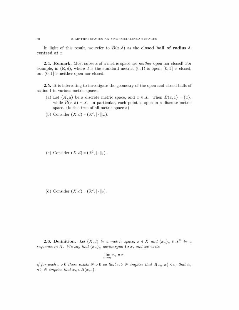
2.5. It is interesting to investigate the geometry of the open and closed balls ofradius 1 in various metric spaces.

(a) Let (X,µ) be a discrete metric space, and x ∈ X. Then B(x,1) = x,while B(x, δ) = X. In particular, each point is open in a discrete metricspace. (Is this true of all metric spaces?)

(b) Consider (X,d) = (R2, ∥ ⋅ ∥∞).

(c) Consider (X,d) = (R2, ∥ ⋅ ∥1).

(d) Consider (X,d) = (R2, ∥ ⋅ ∥2).

2.6. Definition. Let (X,d) be a metric space, x ∈ X and (xn)n ∈ XN be asequence in X. We say that (xn)n converges to x, and we write

limn→∞

xn = x,

if for each ε > 0 there exists N > 0 so that n ≥ N implies that d(xn, x) < ε; that is,n ≥ N implies that xn ∈ B(x, ε).


We say that the sequence (xn)n is Cauchy if for all ε > 0 there exists N > 0 sothat m,n ≥ N implies

d(xn, xm) < ε.

As is the case for sequences of real numbers, every convergent sequence in ametric space is Cauchy. The proof is identical to the real case, and is left as anexercise.

The following familiar result from Calculus holds in the more general setting ofmetric spaces.

2.7. Proposition. Let (X,d) be a metric space, and suppose that (xn)n is aCauchy sequence in X. Suppose that there exists a subsequence (xnk)

∞k=1 of (xn)n

and an element x ∈X so thatlimk→∞

xnk = x.

Then limn xn = x.Proof. See the homework problems.

◻

2.8. Example. Let (xn)n be a sequence in a discrete metric space (X,µ). Thenlimn xn = x if and only if there exists N > 0 so that n ≥ N implies that xn = x.

Indeed,

Suppose that there exists N > 0 so that n ≥ N implies that xn = x. Givenany ε > 0, n ≥ N implies that d(xn, x) = 0 < ε, and so limn xn = x.

Now suppose that limn xn = x. Let 0 < ε ≤ 1, and choose N > 0 so thatn ≥ N implies that d(xn, x) < ε. Then n ≥ N implies that xn = x.

2.9. Example. Let X = C([0,1],R). Consider the sequence (fn)n, where

fn(x) =

⎧⎪⎪⎪⎪⎨⎪⎪⎪⎪⎩

2nx x ∈ [0, 12n]

2 − 2nx x ∈ [ 12n ,

1n]

0 x ∈ [ 1n ,1].

Then

(fn)n converges pointwise to 0. That is, for each x ∈ [0,1], limn fn(x) = 0.Indeed, fn(0) = 0 for all n ≥ 1, and so clearly limn fn(0) = 0. If 0 < x ≤ 1,

then there exists N > 0 so that 1N < x, and then n ≥ N implies that

fn(x) = 0, so that limn fn(x) = 0 as well.


(fn)n converges to 0 in (C([0,1],R), ∥ ⋅ ∥1).Consider

d1(fn,0) ∶= ∥fn − 0∥1 = ∫

1

0∣fn(x)∣dx =

1

2n.

Since limn1

2n = 0, it follows that (fn)n converges to 0 in (C([0,1],R), ∥ ⋅∥1). (fn)n does not converge in (C([0,1],R), ∥ ⋅ ∥∞).

It suffices to prove that (fn)n is not Cauchy. Let 0 < ε ≤ 1, and supposethat N ≥ 1. Choose m,n ≥ N with m > 2n. Then fm( 1

2n) = 0 and fn(1

2n) =

1, so

d∞(fn, fm) = ∥fn − fm∥∞ ≥ ∣fn(1

2n) − fm(

1

2n)∣ = 1,

proving that (fn)n is not Cauchy in (C([0,1],R), ∥ ⋅ ∥∞).

2.10. Remark. Convergence in (C([0,1],K), ∥ ⋅ ∥∞) is also referred to as uni-form convergence.

We leave it as an exercise for the reader to prove that if a sequence (fn)n inC([0,1],K) converges uniformly to f , then (fn)n converges pointwise to f , and also(fn)n converges in (C([0,1],K), ∥ ⋅ ∥1).

2.11. Definition. Let (X,d) be a metric space and E ⊆X.A point q ∈X is said to be a limit point of E if there exists a sequence (xn)n ∈

EN such that limn xn = q.We say that the point p ∈ X is an accumulation point of E if for every

neighbourhood H of p, the punctured neighbourhood H ∖ p of p intersects Enon-trivially. That is,

(H ∖ p) ∩E /= ∅.

We write E′ for the set of all accumulation points of E. (This is sometimesreferred to as the derived set of E.)

If q ∈ E and q is not an accumulation point of E, then q is said to be an isolatedpoint of E.

Remarks: in checking that p is an accumulation point of E, it suffices to considerpunctured neighbourhoods of the form B(p, δ) ∖ p. (Why?)

Secondly, it is a routine exercise to prove that if E1 ⊆ E2 ⊆X, then E′1 ⊆ E

′2.

Exercise. Every accumulation point of E in (X,d) is a limit point of E.

2.12. Example. Let (X,µ) be a discrete metric space and E ⊆ X. If p ∈ Xand ε = 1

2 , then either

(a) p ∈ E and B(p, ε) ∩E = p, or(b) p /∈ E, and B(p, ε) ∩E = ∅.

Either way, we see that p is not an accumulation point of E. If p ∈ E, then p mustbe an isolated point of E.


2.13. Example. Consider R with the standard metric d. Let E = 1n

∞n=1.

If p = 0, then for each ε > 0, we can find n > 1ε , so that

(B(0, ε) ∖ 0) ∩E ⊇ 1

n /= ∅.

Hence p = 0 is an accumulation point of E. Note that 0 /∈ E.We leave it as an exercise for the reader to prove that every point of E is an

isolated point of E.

2.14. Theorem. Let (X,d) be a metric space and F ⊆ X. The following areequivalent:

(a) F is closed.(b) F ′ ⊆ F ; that is, every accumulation point of F lies in F .(c) Every limit point of F lies in F .

Proof.

(a) implies (b):Suppose that F is closed and that y ∈ F ′. If y /∈ F , then y ∈ G ∶=X ∖F ,

and so there exists δ > 0 so that B(y, δ) ⊆ G. Then

(B(y, δ) ∖ y) ∩ F ⊆ G ∩ F = ∅,

contradicting the fact that y is an accumulation point of F . Thus y ∈ F ,as required.

(b) implies (c): Suppose that F ′ ⊆ F , and let q be a limit point of F . Let(xn)n be a sequence in F such that limn xn = q. If there exists n ≥ 1 so thatxn = q, then q ∈ F and we are done. Otherwise, let δ > 0, and choose N > 0so that n ≥ N implies that d(xn, q) < δ, i.e. xn ∈ B(q, δ). Since xN /= q, xNlies in the punctured neighbourhood (B(q, δ) ∖ q) of q. Since δ > 0 wasarbitrary, this shows that q is an accumulation point of F , and hence liesin F by our hypothesis in (b).

Hence F contains all of its limit points.(c) implies (a): Suppose that F contains all of its limit points, and let G =

X ∖F . We shall prove that G is open, which is equivalent to showing thatF is closed.

Let y ∈ G. Since y is not a limit point of F , there exists δ > 0 so thatB(y, δ) ∩ F = ∅. But then G is open, so F is closed.

◻

2.15. Example. Let X = R, equipped with the standard metric d. Let H =

1n

∞n=1. Then H is not closed, since 0 ∈H ′ is an accumulation point of H, but 0 /∈H.We note that H is not open, either, since there does not exist δ > 0 so that

B(1, δ) ⊆H.


2.16. Example. Let X = Cb(R,R), equipped with the supremum norm ∥ ⋅ ∥∞.For each n ≥ 1, define

fn(x) =

⎧⎪⎪⎪⎪⎨⎪⎪⎪⎪⎩

0 if x ≤ n;

x − n if n < x ≤ n + 1

1 if n + 1 ≤ x.

It is easy to verify that fn ∈ Cb(R,R) for all n ≥ 1. Let H = fn∞n=1.

Then ∥fn − fm∥∞ = 1 for all 1 ≤ n /= m, and so H ′ = ∅ (why?). In particular, His closed, since H ′ = ∅ ⊆H.

2.17. Theorem. Let (X,d) be a metric space.

(a) If Gλ ⊆X is open for all λ ∈ Λ, then

G = ∪λ∈ΛGλ

is open.(b) If Fλ ⊆X is closed for all λ ∈ Λ, then

F = ∩λ∈ΛFλ

is closed.(c) If n ≥ 1 is an integer and G1,G2, ...,Gn are open in X, then

H = ∩nk=1Gk

is open.(d) If n ≥ 1 is an integer and F1, F2, ..., Fn are closed in X, then

K = ∪nk=1Fk

is closed.

Proof.

(a) Let x ∈ G. Then there exists α ∈ Λ so that x ∈ Gα. Since Gα is open, thereexists δ > 0 so that B(x, δ) ⊆ Gα ⊆ G. Hence G is open.

(b) Set Gλ = X ∖ Fλ for all λ ∈ Λ, so that each Gλ is open. By part (a),G = ∪λ∈ΛGλ is open. Hence F =X ∖G is closed.

(c) Let x ∈ H. Then x ∈ Gk, 1 ≤ k ≤ n. Since each Gk is open, there existδk > 0, 1 ≤ k ≤ n, so that B(x, δk) ⊆ Gk. Let δ = min(δ1, δ2, ..., δn) > 0. Then

B(x, δ) ⊆ B(x, δk) ⊆ Gk,1 ≤ k ≤ n,

and so B(x, δ) ⊆H. Hence H is open.(d) The proof is analogous to that of (b) and is left as an exercise.

◻

2.18. Remark. In parts (c) and (d) of Theorem 2.17, the fact that n is finiteis crucial. For example, if we set X = R, equipped with the standard metric d, andif Gn = (−1, 1

n), n ≥ 1, then each Gn is open in (R, d), but H = ∩n≥1Gn = (−1,0] isneither open nor closed.


2.19. Definition. Let (X,d) be a metric space and H ⊆ X. We define theclosure of H to be

H ∶= ∩F ⊆X ∶H ⊆ F and F is closed.

It should be clear from the definition of H that

H ⊆H. H is closed, being the intersection of closed sets. H is the smallest closed set containing H, in the sense that if K ⊆ X is

closed and H ⊆K, then H ⊆K.

2.20. Proposition. Let (X,d) be a metric space and H ⊆X. Then

(a) H is closed if and only if H =H, and(b) H =H ∪H ′.

In particular, every point of H is a limit point of H.Proof.

(a) Suppose that H = H. By the comments following Definition 2.19, H isclosed and thus H is closed.

Conversely, suppose that H is closed. Now H ⊆ H always holds. Onthe other hand, H is a closed set which contains H, and thus - by the thirdcomment following Definition 2.19, H ⊆H. Hence H =H.

(b) Let K =H ∪H ′.Step One: First we shall prove thatK is closed, by showing thatG =X∖Kis open.

Indeed, suppose that x ∈ G. Then x is not an accumulation point ofH, so there exists δ > 0 so that (B(x, δ)∖ x)∩H = ∅. But x /∈K impliesthat x /∈H either, so

B(x, δ) ∩H = ∅.

Suppose that there exists y ∈ H ′ so that y ∈ B(x, δ). Then ρ ∶= d(x, y) < δ.Since y ∈H ′ is an accumulation point of H, we can find z ∈H ∖y so thatz ∈ B(y, ε), where ε = δ − ρ > 0.

By the triangle inequality,

d(x, z) ≤ d(x, y) + d(y, z) < ρ + ε = δ,

so that z ∈ B(x, δ) ∩H = ∅, a contradiction.Hence

B(x, δ) ∩H ′= ∅.

It follows that B(x, δ) ⊆ G, and so G is open, i.e. K is closed.

Step Two: Since K =H ∪H ′ is closed and H ⊆K, it follows that H ⊆K.Conversely, H is closed and H ⊆ H, so by Theorem 2.14 and the com-

ments following Definition 2.11, H ⊇ (H)′ ⊇ H ′. Thus H ⊇ H ∪H ′ = K, sothat H =K =H ∪H ′.


Finally, if x ∈H, then either x ∈H, in which case, x = limn xn, where xn = x ∈Hfor all n ≥ 1, or x /∈H, in which case x is an accumulation point of H by (b).

◻

2.21. Example. Let X = R2 with the Euclidean metric d2(x, y) = ∥x − y∥2.Then

B((0,0),1) = B((0,0),1)

= (y1, y2) ∈ R2∶ ∥(y1, y2) − (0,0)∥2 ≤ 1

= (y1, y2) ∈ R2∶√

∣y1 − 0∣2 + ∣y2 − 0∣2 ≤ 1.

2.22. Example. Let X = R with the usual metric. If H = Q, then H = R = X,since every point of R is an accumulation point of Q.

2.23. Definition. A subset Y of a metric space (X,d) is said to be dense ifY =X. If X admits a countable dense subset, then X is said to be separable.

2.24. Example. With X = R and d the usual metric, the set I = R ∖ Q ofirrational numbers is dense, and uncountable. However, we saw in Example 2.22that the set Q of rational numbers is also dense in R, and Q is countable, so R isseparable.

Exercise. Suppose that (X,µ) is a discrete metric space. Which are the densesubsets of X? When is (X,µ) separable?

CHAPTER 3

Topology

1. Topological spaces

What I am looking for is a blessing not in disguise.

Jerome K. Jerome

1.1. Definition. Let ∅ /=X be a non-empty set. A subset τ ⊆ P(X) is called atopology on X, and (X,τ) is said to be a topological space, if

(a) ∅,X ∈ τ ;(b) ∪λ∈ΛTλ ∈ τ whenever Tλλ∈Λ ⊆ τ ;(c) ∩nk=1Tk ∈ τ whenever Tk

nk=1 ⊆ τ .

The elements of τ are said to be τ-open - or, if τ is fixed, just open. A subsetF ⊆X is said to be closed if G =X ∖ F ∈ τ .

1.2. Example. Let (X,d) be a metric space. Consider

τ ∶= G ⊆X ∶ for all x ∈ G there exists δ > 0 so that B(x, δ) ⊆ G.

Clearly ∅ and X belong to τ . Also, by Theorem 2.17, conditions (b) and (c) fromDefinition 1.1 also hold. Thus τ is a topology on X, called the metric topologyon X.

Observe that we have defined the metric topology on X so that a set G is openin the sense of Definition 2.2.1 for metric spaces if and only if it is open in thetopological sense of Definition 1.1 above.

If X = K and d is the standard metric on X, then we refer the metric topologyinduced by d as the standard topology on X. Unless otherwise specified, this willbe the metric we shall always consider for K.

37

38 3. TOPOLOGY

1.3. Examples.

(a) Let X be any non-empty set. Then τ = ∅,X is a topology on X, calledthe trivial topology on X.

(b) At the other extreme: Let X be any non-empty set. Then τ = P(X) isa topology on X, called the discrete topology on X. Note that this isthe metric topology induced on X when X is equipped with the discretemetric µ.

(c) Let X = a, b, and set τ = ∅,a,a, b. Then τ is a topology on X.

Question: does there exist a metric d on X so that τ is the metric topologyinduced by d?

(d) Let X = Z and set τ = ∅ ∪ T ⊆ Z ∶ 5 ∈ T. Then τ is a topology on Z.

1.4. Example. Let X be any non-empty set. Define

τcf(X) = ∅ ∪ T ⊆X ∶ ∣X ∖ T ∣ <∞.

Then τcf(X) defines a topology on X, called the co-finite topology.

Borrowing shamelessly from our metric space notions, we obtain the following:

1.5. Definition. Let (X,τ) be a topological space and H ⊆X. The closure ofH is

H = ∩F ⊆X ∶H ⊆ F and F is closed.

We also say that a subset D ⊆ X is dense in X if D = X, and that X isseparable if X admits a countable, dense subset.

As was the case for metric spaces, we see that H is therefore the smallest closedsubset of X which contains H, in the sense that it is contained in every closed subsetof X which contains H.

1.6. Examples.

(a) Suppose that X is a non-empty set equipped with the trivial topology τ .If H = ∅ ⊆ X, then H = ∅ = H, so H is closed. If H /= ∅, then H = X. Inparticular, by taking H to be a singleton set, we see that (X,τ) is separable.

(b) Let X = a, b, and τ = ∅,a,a, b. Then ∅ = ∅;

a = a, b;

b = b;

a, b = a, b.(c) Let X = Z and let τ = ∅ ∪ H ⊆ Z ∶ 5 ∈H.

If A = 5,7, then A = Z; If A = 2N, then A = A = 2N.

1. TOPOLOGICAL SPACES 39

1.7. Definition. Let (X,τ) be a topological space and x ∈ X. A neighbour-hood of x is a set U ⊆ X for which there exists G ∈ τ such that x ∈ G ⊆ U . Thecollection

Ux = U ∶ U is a neighbourhood of x

is called the neighbourhood system at x.

Remark: Some authors require neighbourhoods to be open. We do not.

1.8. Example. This notion of a neighbourhood is consistent with our previousnotion of a neighbourhood in a metric space. Thus if (X,d) is a metric space andx ∈ X, then U is a neighbourhood of x if and only if there exists δ > 0 so thatB(x, δ) ⊆ U .

1.9. Theorem. Let (X,τ) be a topological space and x ∈X.

(a) If U ∈ Ux, then x ∈ U .(b) If U,V ∈ Ux, then U ∩ V ∈ Ux.(c) If U ∈ Ux, then there exists V ∈ Ux such that U ∈ Uy for each y ∈ V .(d) If U ∈ Ux and U ⊆ V , then V ∈ Ux.(e) The set G ∈ τ if and only if G contains a neighbourhood of each of its

points.

Conversely: suppose that Y is a non-empty set and for each x ∈ Y we are givena non-empty collection Ux ⊆ P(Y ) satisfying conditions (a) through (d). Supposefurthermore that we declare a set G ∈ Y to be open if for each x ∈ G there existsU ∈ Ux so that x ∈ U ⊆ G. If we then set ρ = G ⊆ Y ∶ G is open, then ρ is a topologyon Y in which the neighbourhood system at x is exactly Ux.Proof.

(a) This is clear from the definition.(b) Let G1,G2 ∈ τ such that x ∈ G1 ⊆ U and x ∈ G2 ⊆ V . Then G = G1 ∩G2 ∈ τ ,

and x ∈ G ⊆ (U ∩ V ), so U ∩ V ∈ Ux.(c) Choose G ∈ τ so that x ∈ G ⊆ U , and set V = G. If y ∈ V , then y ∈ G ⊆ U ,

so U ∈ Uy.(d) Choose G ∈ τ so that x ∈ G ⊆ U . Then x ∈ G ⊆ V , so V ∈ Ux.(e) First suppose that G ∈ τ , and let x ∈ G. Then x ∈ G ⊆ G, so G ∈ Ux.

Hence G is itself a neighbourhood of each of its points. Conversely, suppose that G contains a neighbourhood of each of its

points. Let x ∈ G. Then there exists Tx ∈ τ so that x ∈ Tx ⊆ G. Butthen

G = ∪x ∶ x ∈ G ⊆ ∪Tx ∶ x ∈ G ⊆ G,

and thus G = ∪Tx ∶ x ∈ G. Since the union of open sets is open,G ∈ τ .

Next, suppose that ∅ /= Y is a set satisfying (a)-(d), and that we have defined ρas in the statement of the Theorem.

40 3. TOPOLOGY

It is clear that ∅ belongs to ρ trivially.As for Y , note that for each y ∈ Y , we have that Uy ≠ ∅ (by hypothesis).

Hence there exists Uy ∈ Uy and by hypothesis (a), y ∈ Uy. But then for ally ∈ Y , y ∈ Uy ⊆ Y , and thus Y is declared open.

Suppose that Tλ ∈ ρ, λ ∈ Λ. Let T = ∪λ∈ΛTλ, and choose x ∈ T . Then x ∈ Tλ0for some λ0 ∈ Λ, and so there exists U ∈ Ux so that x ∈ Ux ⊆ Tλ0 ⊆ T . ThusT is open, i.e. T ∈ ρ.

Suppose that T1, T2, ..., Tn ∈ ρ and let x ∈ T = ∩nk=1Tk. Fix 1 ≤ k ≤ n. Sincex ∈ Tk ∈ ρ, we may find Uk ∈ Ux so that x ∈ Uk ⊆ Tk. By (finite) inductionusing condition (b), Ux = ∩

nk=1Uk ∈ Ux, and clearly

x ∈ Ux ⊆ T.

But x ∈ T was arbitrary, so T ∈ ρ by definition of ρ.

Thus ρ is a topology. We leave the last statement as an exercise for the reader. Theproof can be found in the appendix to this Chapter.

◻

1.10. Definition. Let (X,τ) be a topological space. A directed set is a set Λwith a relation ≤ that satisfies:

(i) λ ≤ λ for all λ ∈ Λ;(ii) if λ1 ≤ λ2 and λ2 ≤ λ3, then λ1 ≤ λ3; and(iii) if λ1, λ2 ∈ Λ, then there exists λ3 so that λ1 ≤ λ3 and λ2 ≤ λ3.

The relation ≤ is called a direction on Λ.A net in X is a function P ∶ Λ→X, where Λ is a directed set. The point P (λ)

is usually denoted by xλ, and we often write (xλ)λ∈Λ to denote the net.A subnet of a net P ∶ Λ → X is the composition P ϕ, where ϕ ∶M → Λ is an

increasing cofinal function from a directed set to Λ; that is,

(a) ϕ(µ1) ≤ ϕ(µ2) if µ1 ≤ µ2 (increasing), and(b) for each λ ∈ Λ, there exists µ ∈M so that λ ≤ ϕ(µ) (cofinal).

For µ ∈M , we often write xλµ for P ϕ(µ), and speak of the subnet (xλµ)µ.

Remark: It might be worth recalling that a sequence in a set X defined to be afunction f ∶ N → X, and that we normally write xn instead of f(n), and (xn)

∞n=1

instead of f . Thus, our notation (xλ)λ∈Λ for a net has been chosen to mimic thenotation we use for sequences. The same is true of our definition of convergence fornets, which mimics the definition of convergence in a metric space.

1.11. Definition. Let (X,τ) be a topological space. The net (xλ)λ is said toconverge to x ∈ X if for every U ∈ Ux there exists λ0 ∈ Λ so that λ ≥ λ0 impliesxλ ∈ U .

We write limλ xλ = x, or limλ∈Λ xλ = x.

1. TOPOLOGICAL SPACES 41

1.12. Examples.

(a) Since N is a directed set under the usual order ≤, every sequence is a net.Any subsequence of a sequence is also a subnet. The converse to this isfalse, however. A subnet of a sequence need not be a subsequence, sinceits domain need not be N (or any countable set, for that matter).

(b) Let A be a non-empty set and Λ denote the power set of all subsets of A,partially ordered with respect to inclusion. Then Λ is a directed set, andany function from Λ to R is a net in R.

(c) Let P denote the set of all finite partitions of [0,1], partially ordered byinclusion (i.e. refinement). Let f be a continuous function on [0,1]; thento P = 0 = t0 < t1 < ⋯ < tn = 1 ∈ P, we associate the quantity LP (f) =

∑ni=1 f(ti−1)(ti − ti−1). The map P ↦ LP (f) is a net (P is a directed set),

and from Calculus, limP ∈P LP (f) = ∫1

0 f(x)dx.Indeed, if we let ε > 0, then by the fact that every continuous function

is Riemann integrable, we know that there exists a partition P0 ∈ P so that

∫1

0 f(t)dt − ε < LP0(f) ≤ ∫1

0 f(t)dt. But then for any refinement P of P0

(i.e. P0 ⊆ P ∈ P), we have

∫

1

0f(t)dt − ε < LP0(f) ≤ LP (f) ≤ ∫

1

0f(t)dt,

and therefore P ≥ P0 implies LP (f) ∈ (∫1

0 f(t)dt − ε, ∫1

0 f(t)dt + ε). This is

precisely the statement that limP ∈P LP (f) = ∫1

0 f(x)dx.(d) Let F = F ⊆ N ∶ ∣F ∣ < ∞. We partially order F by inclusion: F1 ≤ F2 if

F1 ⊆ F2.Given F1, F2 ∈ Λ, F3 = F1 ∪F2 ∈ F and F1 ≤ F3, F2 ≤ F3. Thus (F ,≤) is

a directed set.Consider X = R, equipped with the standard topology. For each F ∈ F ,

define xF = 1∣F ∣+1 ∈ R. Then (xF )F ∈F is a net in R.

Suppose that U ∈ U0 is a neighbourhood of 0 in R. Then there existsδ > 0 so that (−δ, δ) ⊆ U . Choose N > 0 so that 1

N < δ. Fix F0 ∈ F with

∣F0∣ ≥ N . If F ∈ F and F ≥ F0, then ∣F ∣ ≥ ∣F0∣ ≥ N , so ∣xF − 0∣ = 1∣F ∣+1 ≤

1N+1 < δ. Thus

limF ∈F

xF = 0.

1.13. Example. Let (X,τX) be a topological space and x ∈ X. Let Ux denotethe nbhd system at x. If, for U1, U2 ∈ Ux we define the relation U1 ≤ U2 if U2 ⊆ U1,then (Ux,≤) forms a directed set.

For each U ∈ Ux, choose xU ∈ U . Then (xU)U∈Ux forms a net in X. It is not hardto see that limU∈Ux xU = x. Indeed, given V ∈ Ux, we have that xU ∈ V for all U ≥ V .

1.14. Definition. Let (X,τX) and (Y, τY ) be topological spaces. We say thata function f ∶X → Y is continuous if f−1(G) is open in X for all G ∈ τY .

42 3. TOPOLOGY

That this extends our usual notion of continuity for functions between metricspace is made clear by the following result:

1.15. Proposition. If (X,dX) and (Y, dY ) are metric spaces with metric spacetopologies τX and τY respectively, then the following are equivalent for a functionf ∶X → Y :

(a) f is continuous on X, i.e. f−1(G) ∈ τX for all G ∈ τY .(b) limn f(xn) = f(x) whenever (xn)

∞n=1 is a sequence in X converging to x ∈X.

Proof. See Assignment.

◻

As we shall see in the Assignments, sequences are not enough to describe conver-gence, nor are they enough to characterize continuity of functions between generaltopological spaces. On the other hand, nets are sufficient for this task, and serveas the natural replacement for sequences. (The following result also admits a localversion, which we shall also see in the Assignments.)

1.16. Theorem. Let (X,τX) and (Y, τY ) be topological spaces. Let f ∶ X → Ybe a function. The following are equivalent:

(a) f is continuous on X.(b) Whenever (xλ)λ∈Λ is a net in X which converges to x ∈ X, it follows that

(f(xλ))λ∈Λ is a net in Y which converges to f(x).

Proof. See Assignment.

◻

2. A characterization of compactness for metric spaces

2.1. The notion of compactness should be viewed as a generalization of “finite-ness”.

2.2. Definition. Let (X,τ) be a topological space and E ⊆ X. A collectionHγγ∈Γ is said to be a cover of E if E ⊆ ∪γ∈ΓHγ. The cover is said to be open ifeach Hγ ∈ τ , γ ∈ Γ.

Given a cover of E as above, a finite subcover of E is a finite subcollectionHγk

nk=1 of Hγγ∈Γ so that E ⊆ ∪nk=1Hγk .

Finally, a subset K ⊆X is said to be compact if every open cover of K admitsa finite subcover.

2.3. Example. Suppose that (X,τ) is a topological space and that F ⊆ X isfinite. Then F is compact.

2. A CHARACTERIZATION OF COMPACTNESS FOR METRIC SPACES 43

2.4. Theorem. Consider R, equipped with the standard topology. If a < b ∈ R,then [a, b] is compact.Proof. We argue by contradiction. Assume otherwise, and let Gλλ∈Λ be an opencover of [a, b] which admits no finite subcover. Let I1 = [a, b].

We split I1 into two subintervals J1,1 and J1,2 of equal length (i.e. J1,1 = [a, c]and J1,2 = [c, b], where c = (a+b)/2. Either J1,1 or J1,2 can not be covered by finitelymany of the Gλ’s (otherwise the union of the finitely many Gλ’s would cover I1).

If J1,1 can not be so covered, set I2 = J1,1. Otherwise, let I2 = J1,2. We nowproceed inductively. Given Ik = [ak, bk] which can not be covered by finitely manyof the Gλ’s, set Jk,1 = [ak, ck] and Jk,2 = [ck, bk], where ck = (ak + bk)/2. One of Jk,1,Jk,2 can not be covered by finitely many of the Gλ’s. If Jk,1 cannot be so covered,set Ik+1 = Jk,1, otherwise set Ik+1 = Jk,2. Write Ik+1 = [ak+1, bk+1].

Observe that

I1 ⊇ I2 ⊇ I3 ⊇ ⋯,

and that diam Ik ∶= (bk − ak) = b−a2k−1

converges to 0 as k tends to infinity. Thus∩∞k=1Ik = z, a single point (by the Nested Intervals Theorem). (Recall that z =

limk ak = supk ak = infk bk = limk bk.) Now, z ∈ [a, b] ∈ ∪λ∈ΛGλ, and so z ∈ Gλ0 forsome λ0 ∈ Λ.

Since Gλ0 is open, there exists δ > 0 so that (z − δ, z + δ) ⊆ Gλ0 . But then if m issufficiently large, Im ⊆ (z − δ, z + δ) ⊆ Gλ0 , contradicting the fact that Im could notbe covered by finitely many of the Gλ’s.

Thus [a, b] must be compact.

◻

2.5. Example. Consider R, equipped with the standard topology. Then E =

(0,1] is not compact. For example, if we let Gx = (x,2), x ∈ (0,1), then Gxx∈(0,1)is an open cover of E which does not admit a finite subcover.

2.6. Examples.

(a) Let (X,τ) be a space endowed with the trivial topology τ = ∅,X. Thenevery subset K ⊆X is compact.

(b) Let (X,µ) be a space endowed with the discrete topology. Then K ⊆ X iscompact if and only if K is finite.

2.7. Definition. Let (X,τ) be a topological space, and suppose that Y ⊆ X.The relative topology on Y inherited from X is

τY ∶= G ∩ Y ∶ G ∈ τ.

We say that H ∈ τY is relatively open in Y . Similarly, K ⊆ Y is relatively closedin Y if Y ∖K is relatively open in Y .

We leave it as an exercise for the reader to show that this is indeed a topologyon Y .

44 3. TOPOLOGY

2.8. Example. Suppose that (X,τ) is a topological space and that Y ⊆ X isopen. Then

τY = G ∩ Y ∶ G ∈ τ = H ⊆ Y ∶H ∈ τ.

That is, H ∈ τY if and only if H ⊆ Y and H is open in X.

2.9. Example.

(a) Consider R equipped with the standard topology τ . Let Z ⊆ R. For anyn ∈ Z,

n = (n − 1, n + 1) ∩Z ∈ τZ.

That is, each point is open in Z in the relative topology. It follows thatif A ⊆ Z, then A = ∪n∈An is a union of open sets, so every subset ofZ is open in the relative topology. That is, the relative topology on Z isthe discrete topology on Z, which coincides with the metric topology on Zinherited from the discrete metric.

(b) Consider R equipped with the standard topology τ , and let Y = (0,1]. Then(0,1/2) is relatively open in Y , since (0,1/2) is open in R and (0,1/2) =(0,1/2) ∩ Y .

More interestingly, (1/2,1] is relatively open in Y , since (1/2,2) is openin R and (1/2,1] = (1/2,2) ∩ Y .

It is clear from the above example that if (X,τ) is a topological space and H ⊆

Y ⊆X, then H may be relatively open in Y without being open in X. Compactness,however, does not depend upon the ambient space.

2.10. Theorem. Let (X,τ) be topological space and Y ⊆ X. Suppose thatK ⊆ Y ⊆X. The following are equivalent:

(a) K is compact as a subset of (X,τ).(b) K is compact as a subset of (Y, τY ).

Proof.

(a) Suppose that K is compact as a subset of (X,τ), and let Hλλ∈Λ be aτY -open cover of K. That is, Hλ ∈ τY for all λ ∈ Λ, and K ⊆ ∪λHλ.

By definition of the relative topology on Y , for each λ ∈ Λ, there existsGλ ∈ τ so that Hλ = Gλ ∩ Y . Thus

K ⊆ ∪λHλ ⊆ ∪λGλ.

Since K is compact in (X,τ), we can find λ1, λ2, ..., λn ∈ Λ so that

K ⊆ ∪nk=1Gλk .

But then

K =K ∩ Y ⊆ (∪nk=1Gλk) ∩ Y = ∪

nk=1(Gλk ∩ Y ) = ∪

nk=1Hλk .

It follows that every τY -open cover of K admits a finite subcover, and soK is compact in (Y, τY ).


(b) Conversely, suppose that K is compact in (Y, τY ) and let Gλλ∈Λ be aτ -open cover of K in X. For all λ, let Hλ = Gλ ∩ Y , so that Hλ ∈ τY .

Since K = K ∩ Y , it follows that K ⊆ ∪λHλ. Since K is compact in(Y, τY ), there exist λ1, λ2, ..., λn ∈ Λ so that

K ⊆ ∪nk=1Hλn ⊆ ∪

nk=1Gλn .

It follows that K is compact in (X,τ).

◻

2.11. Definition. A topological space (X,τ) is said to be Hausdorff or T2 iffor each pair x, y ∈ X with x /= y, there exist neighbourhoods U ∈ Ux and V ∈ Uy sothat U ∩ V = ∅. We also say that x and y can be separated.

2.12. Examples.

(a) Let (X,d) be a metric space and τ denote the metric topology on X inducedby d. If x, y ∈X and x /= y, then β ∶= 1

2 d(x, y) > 0. Also, B(x,β), B(y, β) ∈τ and B(x,β) ∩B(y, β) = ∅. Hence (X,τ) is Hausdorff.

(b) Let X = a, b and τ = ∅,a,X. Then a and b can not be separated,since the only open set which contains b is X itself, which also contains a.Thus X is not Hausdorff.

As we shall see in the Assignments, the Hausdorff property of a topological spaceis what guarantees that limits of nets are unique.

2.13. Theorem. Suppose that (X,τ) is a Hausdorff space and that K ⊆ X iscompact. Then K is closed. In particular, every singleton set in a Hausdorff spaceis closed.Proof. Our goal is to show that M ∶=X ∖K is open. To that end, let x ∈M . SinceX is Hausdorff, for each y ∈K, we can find disjoint neighbourhoods Uy of y and Vyof x. Without loss of generality, we may assume that Uy and Vy are open (why? ).

Thus Uyy∈K is an open cover of K, and since K is compact, we can findy1, y2, ..., yn ∈K so that

K ⊆ ∪nk=1Uyk .

Let V = ∩nk=1Vyk . Then V is open, being the finite intersection of open sets, andV ∩Uyk = ∅, 1 ≤ k ≤ n, which implies that V ∩K = ∅. That is, x ∈ V ⊆M . Hence Mis open, or equivalently, K is closed.

The last statement follows from above, keeping in mind that every finite set ina topological space is compact.

◻

2.14. Corollary. Every compact subset of a metric space is closed in the metrictopology.

46 3. TOPOLOGY

2.15. Proposition. Let (K,τ) be a compact topological space, and F ⊆ K beclosed. Then F is compact.Proof. Let Gλλ∈Λ be an open cover of F in K. Since F is closed, observe thatG =K ∖ F is also open, and that

K = F ∪G ⊆ (∪λGλ) ∪G.

That is, Gλλ ∪ G is an open cover of K. Since K is compact, there existλ1, λ2, ..., λn ∈ Λ so that

K ⊆ (∪nk=1Gλk) ∪G.

But then

F =K ∩ F ⊆ ((∪nk=1Gλk) ∪G) ∩ F ⊆ ∪

nk=1Gλk .

That is, Gλλ∈Λ admits a finite subcover of F .This shows that F is compact.

◻

The duality between open and closed sets in a topological space means that everyproperty which may be described in terms of one admits an equivalent formulationin terms of the other. Let us now derive such a formulation of compactness in termsof closed sets.

2.16. Definition. A collection Fλλ∈Λ is said to have the finite intersec-tion property FIP if every finite subcollection Fλ1 , Fλ2 , ..., Fλn has non-emptyintersection; i.e.

∩nk=1Fλk ≠ ∅.

2.17. Example. For each t ∈ (0,1), consider the set Ht = (t,2) ⊆ R. LetH = Ht ∶ t ∈ (0,1). Then H has the FIP.

2.18. Theorem. Let (X,τ) be a topological space. The following are equivalent.

(a) X is compact.(b) If F = Fλλ∈Λ is a collection of closed subsets of X and F has the FIP,

then

∩λ∈ΛFλ /= ∅.

Proof.

(a) implies (b).Suppose that X is compact. Let F = Fλλ∈Λ be a collection of closed

subsets of X which has the FIP. For all λ ∈ Λ, set Gλ = X ∖ Fλ, so thateach Gλ is open. If, to the contrary, ∩λFλ = ∅, then ∪λGλ = X. Since Xis compact, we can find λ1, λ2, ..., λn ∈ Λ so that X = ∪nk=1Gλk . But then∅ = ∩nk=1Fλk , contradicting the fact that F has the FIP. Thus ∩λ∈ΛFλ /= ∅.


(b) implies (a).Now suppose that (b) holds but that X is not compact. Then there ex-

ists an open cover Gλλ∈Λ which does not admit a finite subcover. LettingFλ = X ∖Gλ, λ ∈ Λ, we see that F = Fλλ∈Λ consists of closed sets, hasthe FIP, and yet ∩λ∈ΛFλ = ∅, contradicting the hypothesis of (b). Thus(b) implies that X is compact.

◻

Using the above result, we get the following extension of the Nested IntervalsTheorem.

2.19. Corollary. Let (X,τ) be a compact topological space, and suppose that

F1 ⊇ F2 ⊇ F3 ⊇ ⋯

is a sequence of non-empty closed subsets of X. Then ∩n≥1Fn /= ∅.

Recall the definition of an accumulation point in a metric space from Defini-tion 2.2.11. Closer inspection shows that the definition did not depend upon themetric in any significant way, and so it extends naturally to topological spaces.

2.20. Definition. Let (X,τ) be a topological space and E ⊆ X. A point x ∈

X is said to be an accumulation point of E if for all U ∈ Ux, the puncturedneighbourhood U ∖x of x intersects E non-trivially. That is, (U ∖x)∩E /= ∅.

As we did in the metric space setting, we denote by E′ the set of accumulationpoints of E.

2.21. Example. Consider N, equipped with the co-finite topology τcf fromExample 1.4.

Let H ⊆ N be any infinite set. We claim that H ′ = N; that is, every point n ∈ Nis an accumulation point of H.

Indeed, let U ∈ Un. Then N ∖ U is finite, and so there exists a positive integerN > 0 so that N + 1,N + 2,N + 3, ... ⊆ U . In particular, if M = max(N,n), thenM + 1,M + 2,M + 3, ... ⊆ U ∖ n

But U ∖n is a punctured nbhd of n, and (U ∖n)∩H ≠ ∅, as H is an infiniteset, and as such it is unbounded.

Since every punctured nbhd of n intersects H non-trivially, n ∈ H ′. Since n ∈ Nwas arbitrarily chosen, H ′ = N.

2.22. Definition. A subset D of a topological space (X,τ) is said to be count-ably compact if every infinite subset of D has an accumulation point in D.

A subset S of (X,τ) is said to be sequentially compact if every sequence inS contains a subsequence which converges to a point in S.

The most general relationship which exists between these different notions ofcompact is the following:

48 3. TOPOLOGY

2.23. Proposition. Let (X,τ) be a topological space and H ⊆X. If H is eithercompact or sequentially compact, then H is countably compact.Proof.

Suppose that H is compact. If H is not countably compact, then theremust exist an infinite subset B of H which does not have an accumulationpoint in H. As such, for each x ∈H, there exists an (open) neighbourhoodUx ∈ Ux so that (Ux ∖ x) ∩ B = ∅, or equivalently, Ux ∩ B ⊆ x. Thecollection Uxx∈H is clearly an open cover of H. Since H is compact, thereexists a finite subcover Uxk

nk=1. But then

B =H ∩B ⊆ ∪nk=1(Uxk ∩B) ⊆ ∪

nk=1xk,

contradicting the fact that B is infinite. Thus H must be countably com-pact.

Suppose that H is sequentially compact. Let B ⊆H be an infinite set. ThenB admits a denumerable subset bk

∞k=1. Since H is sequentially compact,

we can find a subsequence (bkm)∞m=1 of the sequence (bk)∞k=1 and b ∈ H so

that limm bkm = b.Let U ∈ Ub. By definition of convergence, there exists M > 0 so that

m ≥M implies that bkm ∈ U . Since j /= k implies that bj /= bk, at most onebkm can be equal to b, and so U ∖ b intersects B non-trivially. That is, bis an accumulation point of B in H, proving that H is countably compact.

◻

2.24. Example. Let τ be the topology on N generated by the sets Tn =

2n − 1,2n, n ≥ 1. (See the Assignments for the notion of a topology generated bya subbase.)

Let ∅ /=H ⊆ N, and suppose m ∈H.

If m is odd, then m + 1 is an accumulation point of H. Indeed, let G ∈ τand suppose that m + 1 ∈ G. Then m ∈ G. Let U be any neighbourhoodof m + 1. Then U contains an open neighbourhood of m + 1, and so fromabove, m ∈ U . That is, (U ∖ m + 1) ∩H ⊇ m /= ∅.

If m is even, then a similar argument shows that m− 1 is an accumulationpoint of H.

It follows that N is countably compact.

Observe that N is not compact. Indeed, N = ∪∞n=1Tn and each Tn is open (by ourdefinition of τ !), but the cover Tn

∞n=1 does not admit a finite subcover.

Moreover, (N, τ) is not sequentially compact. For example, consider the se-quence (xk)

∞k=1, where xk = k, k ≥ 1. Suppose that there exists m ∈ N and a

subsequence (xkj)∞j=1 so that limj xkj = m. Then there exists m′ ∈ m − 1,m + 1

so that U = m,m′ is an (open) neighbourhood of m. But xkj∞j=1 is not even

bounded, so it cannot be that the tail of the sequence (xkj)j would lie in U , therebyestablishing our claim.


2.25. Remark. We mention in passing that the notions of compactness andof sequential compactness are distinct. It can be shown that there exist compacttopological spaces which are not sequentially compact, and sequentially compacttopological spaces which are not compact. Unfortunately, the proofs of each ofthese statements is beyond the scope of the course.

The standard example of a compact space which is not sequentially compactis obtained by considering an uncountable direct product of the compact interval[0,1], equipped with the so-called product topology.

The standard example of a sequentially compact space which is not compact isobtained by consider the first uncountable ordinal Ω, and imbuing Ω with theorder topology. This is the topology on Ω generated by sets of the form

x ∈ Ω ∶ x < a and x ∈ Ω ∶ x > a

where a ∈ Ω. It follows that the open sets in the order topology are unions of openintervals.

The reader is directed to the excellent book by Stephen Willard for a furtherdiscussion of these topics.

Thus, while compact, sequentially compact and countably compact are, in general,distinct concepts, our goal is to prove that these notions coincide in the setting ofmetric spaces. We first require two more definitions.

2.26. Definition. Let (X,d) be a metric space and let E ⊆ X. A finite setx1, x2, ..., xn ⊆X is called an ε-net for E if

E ⊆ ∪nk=1B(xk, ε).

We say that E is totally bounded if for each ε > 0, E admits an ε-net.

It is not hard to verify that if E ⊆ X is totally bounded and H ⊆ E, then H isalso totally bounded.

2.27. Example. Let I = [0,1] ⊆ R, with the standard metric d(x, y) = ∣x − y∣,x, y ∈ [0,1]. First ε > 0 and choose N > 1

ε . Then

0,1

N,

2

N,⋯,

N − 1

N,1

is an ε-net for I, since I ⊆ ∪Nk=0(kN − ε, kN + ε).

Since ε > 0 was arbitrary, I is totally bounded.

50 3. TOPOLOGY

2.28. Definition. Let (X,d) be a metric space. Given E ⊆ X, the diameterof E is

diamE = supd(x, y) ∶ x, y ∈ E.

We say that E is bounded if diamE <∞.

We leave it to the reader to check that a subset of E ⊆ Rn is bounded in themetric sense if and only if E is bounded in the usual sense.

2.29. Examples.

(a) Consider R2 equipped with the standard (Euclidean) metric

d((x1, y1), (x2, y2)) =√

∣x1 − x2∣2 + ∣y1 − y2∣

2.

Let E = [0,1] × [0,1] = (x, y) ∶ 0 ≤ x, y ≤ 1. Then diamE =√

2 <∞, so Eis bounded.

(b) Let (X,d) be a metric space, x ∈X and ε > 0. Then diamB(x, ε) ≤ 2ε. Tosee this, note that if y, z ∈ B(x, ε), then d(y, z) ≤ d(y, x) + d(x, z) < 2ε.

2.30. Proposition. Let (X,d) be a metric space and E ⊆ X. The followingare equivalent.

(a) E is totally bounded.(b) For every ε > 0, there exists a decomposition E = ⊍

nk=1Ek with diamEk < ε

for all 1 ≤ k ≤ n.

Proof.

(a) implies (b). Suppose that E is totally bounded. Let ε > 0 and let xknk=1

be an ε/2-net for E. Let E1 = B(x1, ε/2), and for k ≥ 2, let

Ek = (B(xk, ε/2) ∖ (k−1

⊍i=1

Ei)) ∩E.

By construction, the Ek’s are disjoint. Also, Ek ⊆ B(xk, ε/2) implies thatdiamEk ≤ diamB(xk, ε/2) ≤ ε, and clearly

∪nk=1Ek = (∪

nk=1B(xk, ε/2)) ∩E = E.

(b) implies (a). Suppose that E satisfies condition (b), and let ε > 0. Choosexk ∈ Ek, 1 ≤ k ≤ n. Then Ek ⊆ B(xk, ε), as diamEk < ε, 1 ≤ k ≤ n. Hence

E =n

⊍k=1

Ek ⊆ ∪nk=1B(xk, ε),

proving that E is totally bounded.

◻


2.31. Proposition. Let (X,d) be a metric space. If X is totally bounded, thenX is bounded.Proof. Let ε = 1 and choose an ε-net xk

nk=1 for X, which exists because X is

totally bounded. Thus X = ⋃nk=1B(xk, ε).

Let ρ = max1≤j,k≤n d(xj , xk). Given x, y ∈ X, there exist 1 ≤ r, s ≤ n so thatx ∈ B(xr, ε) and y ∈ B(xs, ε). Thus

d(x, y) ≤ d(x,xr) + d(xr, xs) + d(xs, y)

≤ ε + ρ + ε

= ρ + 2.

Since ρ + 2 is a fixed constant, X is bounded.

◻

2.32. Example. The converse to Proposition 2.31 is false. To see this, we beginwith a simple observation. Suppose that a metric space (X,d) is totally bounded.Let xk

nk=1 be a 1

2 -net for X, so that

X =n

⋃k=1

B(xk,1

2).

Let m > n, and suppose that y1, y2, ..., ym are m distinct points in X. Then thereexist 1 ≤ i /= j ≤ m so that d(yi, yj) < 1. Indeed, the Pigeonhole Principle implies

that there exist 1 ≤ i /= j ≤ m and 1 ≤ k ≤ n so that yi, yj ∈ B(xk,12). An easy

application of the triangle inequality show that d(yi, yj) < 1.

Consider `∞ (from Example 2.1.7), equipped with the supremum norm

∥(zn)n∥∞ = supn≥1

∣zn∣.

Let X = z = (zn)n ∈ `∞ ∶ ∥z∥∞ ≤ 1 be the unit ball of `∞, and denote by d themetric d(w, z) = ∥w − z∥∞. Given w = (wn)n and z = (zn)n ∈X,

d(w, z) = ∥w − z∥∞ ≤ ∥w∥∞ + ∥z∥∞ ≤ 2.

Thus (X,d) is bounded.

For each k ≥ 1, let ek = (e(k)n )∞n=1, where e

(k)n = 1 if n = k and e

(k)n = 0 otherwise.

It is easily seen that ek ∈X for all k ≥ 1, and if 1 ≤ i /= j, then

d(ei,ej) = ∥ei − ej∥∞ = 1.

From the first paragraph, we see that (X,d) is not totally bounded.

As a second example, suppose that Y is an infinite set, and that µ representsthe discrete metric on Y . Then clearly Y is bounded, since diamY = supµ(y, z) ∶y, z ∈ Y = 1.

However, if 0 < ε < 1, then any open ball B(yk, ε) of radius ε can contain atmost one point of Y (check!), and thus Y does not admit an ε-net. Hence Y is nottotally bounded.

52 3. TOPOLOGY

2.33. Proposition. Suppose that (X,d) is a metric space and that H ⊆ X issequentially compact. Then H is totally bounded.Proof. We argue by contradiction. Suppose that H is not totally bounded. Thenthere exists ε > 0 for which X does not admit an ε-net. Let x1 ∈ X be chosenarbitrarily. Since x1 is not an ε-net for X, X /= B(x1, ε). Choose x2 ∈X∖B(x1, ε).Since x1, x2 is not an ε-net for X, we can find x3 ∈X ∖ (B(x1, ε)⋃B(x2, ε)).

More generally, for n ≥ 2, having chosen x1, x2, ..., xn as above, the fact thatxk

nk=1 is not an ε-net implies that there exists xn+1 ∈X ∖⋃

nk=1B(xk, ε).

Consider the sequence (xn)n in XN. For any 1 ≤ n < m, xm /∈ ⋃m−1k=1 B(xk, ε)

implies that xm /∈ B(xn, ε), and so d(xn, xm) ≥ ε. From this it follows that no subse-quence (xnk)k of (xn)n is Cauchy, and thus no subsequence of (xn)n can converge.This contradicts the hypothesis that H is sequentially compact.

The proof now follows.

◻

2.34. Definition. Let (X,d) be a metric space and E ⊆ X. Suppose thatGλλ∈Λ is a cover of E. We say that δ > 0 is a Lebesgue number for Gλλ∈Λ ifwhenever B ⊆ E and diamB < δ it follows that there exists β ∈ Λ so that B ⊆ Gβ.

2.35. Example. Let I = [0,1] ⊆ R, equipped with the standard metric topol-ogy as in Example 2.27. Let G1 = (−1

2 ,12), G2 = (0,1) and G3 = (1

2 ,32). Clearly

G1,G2,G3 is a cover of I.Let δ = 1

4 , B ⊆ I, and suppose that diamB < δ.If b ∈ B, then either

b ∈ [0, 14], so B ⊆ (−1

4 ,12) ⊆ G1, or

b ∈ (14 ,

34) so B ⊆ (0,1) = G2, or

b ∈ [34 ,1], so B ⊆ (1

2 ,54) ⊆ G3.

This proves that δ = 14 is a Lebesgue number for G1,G2,G3.

2.36. Lemma. (Lebesgue) Let (X,d) be a metric space and H ⊆ X be se-quentially compact. Let G = Gλλ∈Λ be an open cover of H. Then G has a (positive)Lebesgue number.Proof. Suppose otherwise.

Then, for each n ≥ 1, we can find a set Bn ⊆ H so that diamBn <1n , and there

does not exist λ ∈ Λ for which Bn ∈ Gλ. Choose bn ∈ Bn, n ≥ 1. (This uses thecountable version of the Axiom of Choice!) Since H is sequentially compact, thereexists a subsequence (bnk)k of (bn)n which converges to some element h ∈H.

But G is an open cover of H, and so h ∈ Gβ for some β ∈ Λ. Since Gβ is open,

there exists some δ > 0 so that B(h, δ) ⊆ Gβ. Since limk bnk = h, we may find N > 2δ

so that k ≥ N implies that

d(bnk , h) <δ

2.


If k ≥ N , then 1nk

≤ 1k ≤

1N < δ

2 , and for all b ∈ Bnk ,

d(b, h) ≤ d(b, bnk) + d(bnk , h) < diamBnk +δ

2≤

1

nk+δ

2< δ.

Hence b ∈ B(h, δ) ⊆ Gβ, and so Bnk ⊆ Gβ, a contadiction.Thus G has a positive Lebesgue number.

◻

2.37. Theorem. Let (X,d) be a metric space and K ⊆ X. The following areequivalent.

(a) K is compact.(b) K is countably compact.(c) K is sequentially compact.

Proof.

(a) implies (b).This is Proposition 2.23.

(b) implies (c).Let (xn)n be a sequence in K. If (xn)n admits a constant subsequence

(xnk)k, then that subsequence converges to its constant value, which liesin K.

If (xn)n does not admit a constant subsequence, then H = xn∞n=1 is

a denumerable subset of K which admits an accumulation point h ∈K, bycountable compactness of the latter. As we shall see in the Assignments,this implies that there exists a subsequence (xnk)k of (xn)n which convergesto h ∈K.

Thus K is sequentially compact.(c) implies (a).

Suppose that K is sequentially compact, and let G = Gλλ∈Λ be anopen cover of K. By Lebesgue’s Lemma, G admits a positive Lebesguenumber, say ρ > 0. Also, by Proposition 2.33, K is totally bounded.

Next, by Proposition 2.30, we can partition K as K = ⊍nk=1Ek, where

diamEk < ρ for each 1 ≤ k ≤ n. But then by definition of the Lebesguenumber, for each such 1 ≤ k ≤ n, there exists βk ∈ Λ so that Ek ⊆ Gβk , andso

K =n

⊍k=1

Ek ⊆n

⋃k=1

Gβk .

In other words, G admits a finite subcover of K.Thus K is compact.

◻

54 3. TOPOLOGY

2.38. Corollary. Let n ≥ 1 and K ⊆ Rn. Let Rn be equipped with the standard(Euclidean) topology. The following are equivalent.

(a) K is compact.(b) K is sequentially compact.(c) K is closed and bounded.

Proof. That (a) and (b) are equivalent is Theorem 2.37.That (b) and (c) are equivalent is the Heine-Borel Theorem from Math 247.

◻

3. APPENDIX 55

3. Appendix

In this appendix we provide a proof of the last statement of Theorem 3.1.9,which we restate for the convenience of the reader.

Theorem. Let (X,τ) be a topological space and x ∈X.

(a) If U ∈ Ux, then x ∈ U .(b) If U,V ∈ Ux, then U ∩ V ∈ Ux.(c) If U ∈ Ux, then there exists V ∈ Ux such that U ∈ Uy for each y ∈ V .(d) If U ∈ Ux and U ⊆ V , then V ∈ Ux.(e) The set G ∈ τ if and only if G contains a neighbourhood of each of its

points.

Conversely: suppose that Y is a non-empty set and for each x ∈ Y we are givena non-empty collection Ux ⊆ P(Y ) satisfying conditions (a) through (d). Supposefurthermore that we declare a set G ∈ Y to be open if for each x ∈ G there existsU ∈ Ux so that x ∈ U ⊆ G. If we then set ρ = G ⊆ Y ∶ G is open, then ρ is a topologyon Y in which the neighbourhood system at x is exactly Ux.

Our goal is therefore to show that ρ is a topology on Y in which the neighbour-hood system at x is exactly Ux.

Let

ρ = G ⊆ Y ∶ for all g ∈ G there exists U ∈ Ug such that g ∈ U ⊆ G.

First we show that ρ is a topology on Y .

That ∅ ∈ ρ is vacuously true. Also, given that for each x ∈ Y , the familyUx is non-empty, and x ∈ U ⊆ Y for all U ∈ Ux, we see that Y ∈ ρ as well.

Suppose that Gλλ∈Λ ⊆ ρ, and let G = ∪λ∈ΛGλ. Let x ∈ G. Then thereexists α ∈ Λ so that x ∈ Gα. But Gα ∈ ρ, so there exists U ∈ Ux so thatx ∈ U ⊆ Gα ⊆ G.

That is, for all x ∈ G, there exists U ∈ Ux so that x ∈ U ⊆ G, so G ∈ ρ bydefinition of ρ.

Suppose that G1,G2 ∈ ρ and that G = G1 ∩G2. If G = ∅, then G ∈ ρ fromabove. Otherwise, let x ∈ G. Then x ∈ G1, so there exists U1 ∈ Ux so thatx ∈ U1 ⊆ G1. Similarly, x ∈ G2, so there exists U2 ∈ Ux so that x ∈ U2 ⊆ G2.But then U ∶= U1 ∩U2 ∈ Ux by our hypotheses, and so x ∈ U ⊆ G1 ∩G2 = G.

By definition of ρ, G ∈ ρ.

This shows that ρ is a topology on Y . For x ∈ Y , denote by Vx the nhood systemof x in (Y, ρ).

56 3. TOPOLOGY

Suppose that V ∈ Vx. Then x ∈ V and so there exists G ∈ ρ so that

x ∈ G ⊆ V.

But then x ∈ G ∈ ρ implies that there exists U ∈ Ux so that x ∈ U ⊆ G.Hence G ∈ Ux, since U ∈ Ux and U ⊆ G. But then G ∈ Ux and G ⊆ V impliesthat V ∈ Ux.

That is, Vx ⊆ Ux. Conversely, suppose that U ∈ Ux. We wish to show that U ∈ Vx.

Let W = w ∈ U ∶ U ∈ Uw. Note that x ∈ W , so in particular, W ≠ ∅.We shall prove that W ∈ ρ. If we can do this, then W ∈ ρ and x ∈W impliesthat W ∈ Vx. But then W ⊆ U implies that U ∈ Vx, completing the proof.

Indeed, suppose that w ∈W . Then U ∈ Uw and so by condition (c) thereexists Z ∈ Uw so that y ∈ Z implies that U ∈ Uy. We claim that Z ⊆W .

To see this, let y ∈ Z. Then U ∈ Uy, so y ∈ U and U ∈ Uy. By definitionof W , y ∈W , which proves the claim.

Hence, W ⊆ U ⊆ Y , and for all w ∈ W , there exists Z ∈ Uw so thatw ∈ Z ⊆ W . By definition of ρ, this means that W ∈ ρ. As we have seen,this is sufficient to prove the result.

CHAPTER 4

Completeness

1. Completeness and normed linear spaces

Politicians and diapers have one thing in common. They should bothbe changed regularly, and for the same reason.

Jose Maria de Eca de Quieroz

1.1. From the point of view of an analyst, the real numbers are far betterbehaved than the rational numbers. For example, the Intermediate Value Theoremasserts that if f ∶ [a, b] → R is continuous and f(a) ≤ κ ≤ f(b), then there existsd ∈ [a, b] so that f(d) = κ. Such a result fails if we consider a continuous functionf ∶ (Q∩ [a, b])→ R. For example, let f ∶ Q→ R be the function defined by f(q) = q2.Observe that f(0) = 0 and f(2) = 4, and f is continuous on Q (with respect to thestandard topology on Q which it inherits as a subspace of R). Neverthless, theredoes not exist r ∈ Q so that f(r) = 2. Given a non-empty bounded subset of Q,there is no least upper bound for that set which lies in Q.

These are the kinds of properties which makes analysis possible, and it is to thisproperty that we now turn our attention.

1.2. Definition. A subset H of a metric space (X,d) is said to be completeif every Cauchy sequence in H converges to some element of H.

1.3. Examples.

(a) Let n ≥ 1 be an integer, and consider (Kn, d) where d denotes the standard(Euclidean metric)

d((x1, x2, ..., xn), (y1, y2, ..., yn)) =

¿ÁÁÀ

n

∑k=1

∣xk − yk∣2.

Then (Kn, d) is complete, as seen in Math 147/148.(b) Let ∅ /=X be a non-empty set, equipped with the discrete metric µ. Then

(X,µ) is complete. Indeed, suppose that (xn)n is a Cauchy sequence andlet ε = 1. Choose N > 0 so that m,n ≥ N implies that µ(xn, xm) < ε = 1.Then n,m ≥ N implies that xn = xm, or equivalently, n ≥ N implies that

57

58 4. COMPLETENESS

xn = xN . In particular, if δ > 0, then n ≥ N implies that µ(xn, xN) = 0 < δ,proving that limn xn =XN .

(c) The open interval (0,1) ⊆ R when equipped with the standard metric d isnot complete. It is easily seen that ( 1

n)n is a Cauchy sequence which doesnot converge to any element of (0,1).

1.4. Definition. Two topological spaces (X,τX) and (Y, τY ) are said to behomeomorphic if there exists a bijection f ∶ X → Y such that both f and f−1 arecontinuous. When this is the case, we write X ≃ Y .

If X and Y are topological spaces as above and X ≃ Y , then G ∈ τX if andonly if f(G) ∈ τY . Any topological property of X is shared by Y and vice-versa.For example, X is Hausdorff if and only if Y is. Homeomorphism is the notion ofisomorphism in the category of topological spaces.

1.5. Remark. Consider the map

f ∶ R → (−1,1)x ↦ x

1+∣x∣ .

It is readily verified that f is a continuous bijection whose inverse is also contin-uous. Thus R is homeomorphic to (−1,1). It is worth pointing out, however, thatR is complete, while (−1,1) is not.

This shows that completeness is not a topological property of a space.

1.6. Proposition. Let (X,d) be a metric space and H ⊆X be complete. ThenH is closed.Proof. Suppose that x ∈H. Then x is a limit point of H, so there exists a sequence(xn)n in H which converges to x. But then that sequence is Cauchy, and since His complete, x ∈H.

◻

One of the more interesting contexts in which to study completeness is that ofnormed linear spaces.

1.7. Definition. A series ∑n xn in a normed linear space (X, ∥ ⋅ ∥) is said to besummable if there exists x ∈ X such that

limN

∥x −N

∑n=1

xn∥ = 0.

We then write x = ∑n xn.

We say that ∑n xn is absolutely summable if

∑n

∥xn∥ <∞.

1. COMPLETENESS AND NORMED LINEAR SPACES 59

The following result provides a very practical tool when trying to decide whetheror not a given normed linear space is complete. We remark that the second halfof the proof uses the standard fact that if (yn)n is a Cauchy sequence in a metricspace (Y, d), and if (yn)n admits a convergent subsequence with limit y0, then theoriginal sequence (yn)n converges to y0 as well. The proof of this is identical to theproof of the corresponding result in R, and is left as an (important!) exercise forthe reader.

1.8. Theorem. Let (X, ∥⋅∥) be a normed linear space. The following statementsare equivalent:

(a) X is complete, and hence X is a Banach space.(b) Every absolutely summable series in X is summable.

Proof.

(a) implies (b): Suppose that X is complete, and that ∑xn is absolutely

summable. For each k ≥ 1, let yk = ∑kn=1 xn. Given ε > 0, we can find N > 0

so that m ≥ N implies ∑∞n=m ∥xn∥ < ε. If k ≥m ≥ N , then

∥yk − ym∥ = ∥k

∑n=m+1

xn∥

≤k

∑n=m+1

∥xn∥

≤∞∑

n=m+1

∥xn∥

< ε,

so that (yk)k is Cauchy in X. Since X is complete, y = limk→∞ yk =

limk→∞∑kn=1 xn = ∑

∞n=1 xn exists, i.e. ∑∞

n=1 xn is summable.(b) implies (a): Next suppose that every absolutely summable series in X is

summable, and let (yj)j be a Cauchy sequence in X. For each n ≥ 1 thereexists Nn > 0 so that k,m ≥ Nn implies ∥yk − ym∥ < 1/2n+1. Let x1 = yN1

and for n ≥ 2, let xn = yNn − yNn−1 . Then ∥xn∥ < 1/2n for all n ≥ 2, so that

∞∑n=1

∥xn∥ ≤ ∥x1∥ +∞∑n=2

1

2n

≤ ∥x1∥ +1

2<∞.

By hypothesis, y = ∑∞n=1 xn = limk→∞∑

kn=1 xn exists. But

∑kn=1 xn = yNk , so that limk→∞ yNk = y ∈ X. Recalling that (yj)j was

Cauchy, we conclude from the remark preceding the Theorem that (yj)jalso converges to y. Since every Cauchy sequence in X converges, X iscomplete.

◻

60 4. COMPLETENESS

1.9. Definition. Let (X, ∥ ⋅ ∥) be a normed linear space and d be the metric onX induced by the norm. If (X, d) is complete, we say that (X, ∥ ⋅ ∥) is a Banachspace.

Thus a Banach space is a complete normed linear space.

1.10. Theorem. The normed linear space (`1, ∥ ⋅ ∥1) is a Banach space.Proof.

By Theorem 1.8, it suffices to prove that every absolutely summable series in `1is summable.

Suppose that ∑n xn is absolutely summable with M ∶= ∑n ∥xn∥1 < ∞. Writingxn = (xn,k)

∞k=1 for each n ≥ 1, we easily see that each ∣xn,k∣ ≤ ∥xn∥1, and thus for

each k ≥ 1,

∞∑n=1

∣xn,k∣ ≤M <∞.

Since (K, ∣ ⋅ ∣) is complete (from first-year Calculus), the series ∑∞n=1 xn,k is summable

for each k ≥ 1. Define

zk =∞∑n=1

xn,k,

and set z = (zk)∞k=1. We must show that z ∈ `1, and that z = ∑n xn.

z ∈ `1:Consider

∞∑k=1

∣zk∣ ≤∞∑k=1

(∞∑n=1

∣xn,k∣)

=∑n∑k

∣xn,k∣

=∑n

∥xn∥1

=M <∞.

(Note that interchanging the order of summation in the second equation isjustified by the fact that all of the terms are non-negative.)

z = ∑n xn:


Let ε > 0 and choose N > 0 so that m ≥ N implies that ∑∞m=N ∥xn∥1 < ε.

This is possible since the series is absolutely summable. If m ≥ N , then

∥z −m

∑n=1

xn∥1 =∞∑k=1

∣zk −m

∑n=1

xn,k∣

=∞∑k=1

∣∞∑

n=m+1

xn,k∣

≤∞∑k=1

∞∑

n=m+1

∣xn,k∣

=∞∑

n=m+1

∞∑k=1

∣xn,k∣

=∞∑

n=m+1

∥xn∥1

< ε.

Thus z = limm→∞∑mn=1 xn = ∑n xn.

It follows that (`1, ∥ ⋅ ∥1) is complete, i.e. a Banach space.

◻

1.11. Theorem. The normed linear space (`∞, ∥ ⋅ ∥∞) is a Banach space.Proof.

This is an Assignment problem.

◻

1.12. Definition. Let (H, ⟨⋅, ⋅⟩) be an inner product space, and let ∥ ⋅ ∥ denote

the norm induced by the inner product, i.e. ∥x∥ =√

⟨x,x⟩ for all x ∈H.If (H, ∥ ⋅ ∥) is complete, we say that H is a Hilbert space. Thus a Hilbert space

is a complete inner product space.

It follows that every Hilbert space is a Banach space. The converse is false,though it is not trivial to prove. Given a Banach space (X, ∥ ⋅∥), one must show thatthere does not exists any inner product on X which induces the given norm ∥ ⋅ ∥.

1.13. Theorem. The inner product space (`2, ⟨⋅, ⋅⟩) is a Hilbert space.Proof.

As we saw in the Assignments, every inner product space is a normed linearspace.

Again, we suppose that ∑n xn is an absolutely summable series in `2, and set

M ∶=∑n

∥xn∥2 <∞.

As was the case for `1, writing xn = (xn,k)∞k=1, it is easy to see that for each k ≥ 1,

∣xn,k∣ ≤ ∥xn∥2, and thus

∑n

∣xn,k∣ ≤∑n

∥xn∥2 =M <∞.

62 4. COMPLETENESS

As before, the completeness of (K, ∣ ⋅ ∣) implies that zk = ∑∞n=1 xn,k exists for each

k ≥ 1. let z = (zk)∞k=1.

We must show that z ∈ `2 and that z = ∑∞n=1 xn.

The idea behind the following proof is to estimate the quantity which defines∥z − ∑

pn=1 xn∥2, despite the fact that we do not yet know that z ∈ `2! In fact, by

setting p = 0, we shall obtain a proof of the fact that z ∈ `2.

Now for each p ≥ 1, zk −∑pn=1 xn,k = ∑

∞n=p+1 xn,k, and thus

∞∑k=1

RRRRRRRRRRR

∞∑

n=p+1

xn,k

RRRRRRRRRRR

2

≤∞∑k=1

⎛

⎝

∞∑

n=p+1

∣xn,k∣⎞

⎠

2

=∞∑k=1

∞∑

n=p+1

∞∑

m=p+1

∣xn,k∣ ∣xm,k∣

=∞∑

n=p+1

∞∑

m=p+1

(∞∑k=1

∣xn,k∣ ∣xm,k∣)

=∞∑

n=p+1

∞∑

m=p+1

⟨yn, ym⟩,

where for each n ≥ 1, yn = (∣xn,1∣, ∣xn,2∣, ∣xn,3∣, ...) ∈ `2 with ∥yn∥2 = ∥xn∥2. (Again,note that the fact that we can interchange the order of summation as of the thirdline of this equation is due to the fact that all of the terms are non-negative.)

Thus, by the Cauchy-Schwarz Inequality,

∞∑k=1

⎛

⎝

RRRRRRRRRRR

∞∑

n=p+1

xn,k

RRRRRRRRRRR

2⎞

⎠≤

∞∑

n=p+1

∞∑

m=p+1

⟨yn, ym⟩

≤∞∑

n=p+1

∞∑

m=p+1

∥yn∥2 ∥ym∥2

=⎛

⎝

∞∑

n=p+1

∥yn∥2⎞

⎠

2

=⎛

⎝

∞∑

n=p+1

∥xn∥2⎞

⎠

2

.

If p = 0, then this shows that ∑∞k=1 ∣zk∣

2 <∞, and thus z ∈ `2.

More generally, however, if we choose ε > 0 and N > 0 so that p ≥ N implies that

∑∞n=p+1 ∥xn∥2 < ε, then p ≥ N implies that

∥z −p

∑n=1

xn∥2 ≤∞∑

n=p+1

∥xn∥2 < ε.

Thus z = ∑n xn.


By Theorem 1.8 above, (`2, ∥ ⋅ ∥2) is a Banach space, i.e. (`2, ⟨⋅, ⋅⟩) is a Hilbertspace.

◻

1.14. Theorem. The normed linear space (C([0,1],K), ∥ ⋅ ∥∞) is a Banachspace.Proof. We have already seen that C([0,1],K) is a normed linear space whenequipped with the norm

∥f∥∞ = sup∣f(x)∣ ∶ x ∈ [0,1].

There remains to show that it is complete.This follows immediately, however, from the Weierstraß M -test from Math 148,

combined with Theorem 1.8. That is, if we let ∑n fn be an absolutely summableseries of continuous functions on [0,1], then with Mn ∶= ∥fn∥∞, we see that for eachn ≥ 1 we have supx∈[0,1] ∣fn(x)∣ ≤Mn (by definition of Mn) and that ∑nMn <∞ (by

definition of absolute summability).By the Weierstraß M -test, ∑n fn converges uniformly and absolutely to a con-

tinuous function f ∈ C([0,1],K). But uniform convergence is precisely convergencein the ∥ ⋅ ∥∞ norm. By Theorem 1.8, (C([0,1],K), ∥ ⋅ ∥∞) is complete.

◻

For those of you who may not have taken Math 148, an alternative proof of thisis given in the Appendix to this Chapter.

The following is an analogue of the Nested Intervals Theorem for metric spaces.

1.15. Theorem. Let (X,d) be a metric space. The following are equivalent.

(a) (X,d) is complete.(b) If

F1 ⊇ F2 ⊇ F3 ⊇ ⋯

is a nested sequence of closed, non-empty subsets of X and suppose thatlimn diamFn = 0. Then

∩∞n=1Fn /= ∅.

Proof.

(a) implies (b). Suppose that (X,d) is complete.Let (Fn)n be a nest sequence of closed, non-empty subsets of X as

above, withlimn

diamFn = 0.

Fix ε > 0 and choose N > 0 so that n ≥ N implies that diamFn < ε.Choose xn ∈ Fn arbitrarily. If m > n ≥ N , then xm ∈ Fm ⊆ Fn and

xn ∈ Fn, sod(xm, xn) ≤ diamFn < ε.

It follows that (xn)n is a Cauchy sequence in X. Since X is assumed to becomplete, there exists x ∈X so that limn xn = x.

64 4. COMPLETENESS

Note that if p ≥ 1, then n ≥ p implies that xn ∈ Fn ⊆ Fp. From this itfollows that x = limn xn ∈ Fp. But p ≥ 1 was arbitrary, so x ∈ ∩pFp /= ∅.

(b) implies (a). Next, suppose that condition (b) holds, and let (xn)n be aCauchy sequence in X. For each m ≥ 1, set

Fm = xn∞n=m.

Then each Fm is closed, non-empty, and

F1 ⊇ F2 ⊇ F3 ⊇ ⋯.

Furthermore, since (xn)n is Cauchy, given ε > 0, we can find N ≥ 1 so thatm,n ≥ N implies that d(xn, xm) < ε. It follows that diamFN ≤ ε. Butn ≥ N implies that Fn ⊆ FN , so that diamFn ≤ ε for all n ≥ N . This showsthat limn diamFn = 0.

Our hypothesis in (b) implies that ∩nFn /= ∅. Choose x ∈ ∩nFn. Weclaim that limn xn = x. Indeed, if ε > 0 and N are as above, then notingthat for n ≥ N we have xn, x ∈ Fn, we conclude that

d(xn, x) ≤ diamFn ≤ ε.

Hence limn xn = x.

◻

Note that both conditions of the previous Theorem are required.

1.16. Examples.

(a) Let X = R, equipped with the standard metric and Fn = [n,∞), n ≥ 1.Each Fn is closed, and F1 ⊇ F2 ⊇ F3 ⊇ ⋯. Nevertheless, ∩nFn = ∅.

The issue is that limn diamFn =∞ /= 0.(b) LetX = R again and this time set Fn = (0, 1

n]. Now R is complete, Fn ⊇ Fn+1

for all n ≥ 1 and limn diamFn = 0, but ∩nFn = ∅.In this case, the issue is that the Fn’s are not closed.

2. Completions of metric spaces

2.1. Although Q is not complete (with respect to the standard metric), never-theless, Q “sits inside” the complete metric space R. In this section, we make precisewhat we mean by this, and show that every metric space embeds isometrically ina complete metric space. This is extremely useful when studying normed linearspaces.

2. COMPLETIONS OF METRIC SPACES 65

2.2. Definition. A metric space (X∗, d∗) is called a completion of a metricspace (X,d) if

(X∗, d∗) is complete, and (X,d) is isometrically isomorphic to a dense subset of (X∗, d∗); that is,

there exists a map ρ ∶X →X∗ satisfying(i) d∗(ρ(x), ρ(y)) = d(x, y) for all x, y ∈X, and

(ii) X∗ = ρ(X).

2.3. Example. The motivating example is the one we have already mentioned:(R, d) is completion of (Q, d∣Q), where d(x, y) = ∣x − y∣ is the standard metric on Rand d∣Q is the restriction of d to Q ×Q. The map ρ ∶ Q → R defined by ρ(q) = q forall q ∈ Q satisfies the conditions of Definition 2.2 above.

2.4. Our next goal is to show that every metric space has a completion, andthat this completion is in some sense unique. To that end:

let (X,d) be a metric space, and denote by Γ[X] the collection of all Cauchysequences in X. We define a relation ∼ on Γ[X] by setting

(xn)n ∼ (yn)n if and only if limnd(xn, yn) = 0.

Intuitively, under this relation ∼, we identify Cauchy sequences which wouldhave the same limit if that limit existed in X.

2.5. Lemma. With the notation of Section 2.4, the relation ∼ is an equivalencerelation on Γ[X].Proof.

(a) ∼ is reflexive.Clearly (xn)n ∼ (xn)n since limn d(xn, xn) = limn 0 = 0.

(b) ∼ is symmetric.Since d(x, y) = d(y, x) for all x, y ∈ X, it follows that given sequences

(xn)n and (yn)n ∈ Γ[X],

limnd(xn, yn) = lim

nd(yn, xn),

and so (xn)n ∼ (yn)n if and only if (yn)n ∼ (xn)n.(c) ∼ is transitive.

Suppose that (xn)n ∼ (yn)n and that (yn)n ∼ (zn)n. For each n ≥ 1,

d(xn, zn) ≤ d(xn, yn) + d(yn, zn),

and so

0 ≤ limnd(xn, zn) ≤ lim

nd(xn, yn) + lim

nd(yn, zn) = 0 + 0 = 0.

Thus (xn)n ∼ (zn)n, and so ∼ is transitive.

This three properties indicate that ∼ is an equivalence relation.

◻

66 4. COMPLETENESS

2.6. Recall that an equivalence relation ∼ on a set A partitions A into equiva-lence classes.

Let (X,d) be a metric space. We define the set X∗ = Γ[X]/ ∼, so that X∗

consist of the equivalence classes of Cauchy sequences in Γ[X] as determined by theequivalence relation ∼ of Section 2.4.

That is,

X∗= [(xn)n] ∶ (xn)n ∈ Γ[X],

where [(xn)n] denotes the equivalence class of (xn)n under ∼.We define the map:

d∗ ∶ X∗ ×X∗ → R([(xn)n], [(yn)n]) ↦ limn d(xn, yn).

Our first result shows that d∗ is well-defined.

2.7. Proposition. Let (X,d) be a metric space and define X∗, d∗ as in Sec-tion 2.6. Then d∗ is well-defined. That is, if (xn)n ∼ (wn)n and (yn)n ∼ (zn)n, thenlimn d(xn, yn) exists and

limnd(xn, yn) = lim

nd(wn, zn).

Proof. First we check that limn d(xn, yn) exists.Let ε > 0, and choose N > 0 so that m,n ≥ N implies that d(xn, xm) < ε

2 andd(yn, ym) < ε

2 . If m,n ≥ N , then

∣d(xn, yn) − d(xm, ym)∣ ≤ ∣d(xn, yn) − d(xn, ym)∣ + ∣d(xn, ym) − d(xm, ym)∣

≤ d(yn, ym) + d(xn, xm)

<ε

2+ε

2= ε.

Thus (d(xn, yn))n is a Cauchy sequence in R. But R is complete (with the standardmetric), so (d(xn, yn))n converges to some point in R.

Next,

limnd(xn, yn) ≤ lim

nd(xn,wn) + d(wn, zn) + d(zn, yn)

= 0 + limnd(wn, zn) + 0

= limnd(wn, zn),

and by symmetry, limn d(wn, zn) ≤ limn d(xn, yn). Thus we conclude that

limnd(xn, yn) = lim

nd(wn, zn).

◻


2.8. Proposition. The function d∗ defined in Section 2.6 is a metric on X∗.Proof. Suppose that x = [(xn)n], y = [(yn)n] and z = [(zn)n] ∈X

∗. Then

(a) d∗(x, y) = limn d(xn, yn) ≥ 0, since each d(xn, yn) ≥ 0, by virtue of thefact that d is a metric on X. Furthermore, d∗(x, y) = 0 if and only iflimn d(xn, yn) = 0, which by definition happens if and only if (xn)n ∼ (yn)n,ie. if and only if x = y.

(b)

d∗(x, y) = limnd(xn, yn) = lim

nd(yn, xn) = d

∗(y, x),

where the second equality again holds because d is a metric on X.(c)

d∗(x, z) = limnd(xn, zn)

≤ limnd(xn, yn) + d(yn, zn)

= limnd(xn, yn) + lim

nd(yn, zn)

= d∗(x, y) + d∗(y, z),

where the first inequality holds because d is a metric on X, and the secondequality holds because each of the limits exists, as was shown in the previousProposition.

From these three verifications it follows that d∗ is a metric on X∗.

◻

Our next goal is to prove that (X∗, d∗) is a completion of (X,d).

2.9. Proposition. Let (X,d) be a metric space and let (X∗, d∗) be the metricspace of equivalence classes of Cauchy sequences in X modulo the relation ∼ definedin Section 2.6. The map

ρ ∶ X → X∗

x ↦ [(x,x, x, ...)]

is an isometric embedding of X into X∗, and ρ(X) is dense in X∗.Proof. Suppose that x, y ∈X. Then

d∗(ρ(x), ρ(y)) = d∗([(x,x, x, ...)], [(y, y, y, ...)])

= limnd(x, y)

= d(x, y).

From this it follows that ρ is isometric, and hence ρ is injective. Indeed, if x /= y,then d∗(ρ(x), ρ(y)) = d(x, y) > 0, so ρ(x) /= ρ(y).

Next, let z = [(zn)n] ∈ X∗. Let ε > 0. Since (zn)n ∈ Γ[X], it is a Cauchysequence and so we can find N ≥ 1 so that m,n ≥ N implies that d(zn, zm) < ε. Inparticular, d(zn, zN) < ε for all n ≥ N .

68 4. COMPLETENESS

Set y = [(xN , xN , xN , ...)], i.e. set yn = xN for all n ≥ 1. Then

d∗(z, y) = limnd(zn, yn)

= limnd(zn, xN)

≤ ε.

Since y = ρ(xN) ∈ ρ(X) and since ε > 0 is arbitrary, it follows that ρ(X) is dense in(X∗, d∗).

◻

2.10. Theorem. The metric space (X∗, d∗) constructed above is complete, andthus it is a completion of (X,d). In particular, every metric space (X,d) admits acompletion.Proof. Let (βn)n be a Cauchy sequence in X∗, that is; βn = [(xn,k)k≥1] for eachn ≥ 1. Let ρ ∶X →X∗ denote the isometric embedding described above, so that ρ(X)

is dense in X∗. Then we can find a sequence (pn)n in X so that d∗(ρ(pn), βn) <1n ,

n ≥ 1.Note that the fact that (βn)n is Cauchy in X∗ implies that (pn)n is Cauchy in X.

Indeed, if ε > 0 there exists N > 3ε such that m,n ≥ N implies that d∗(βm, βn) <

ε3 .

But then m,n ≥ N implies that

d(pm, pn) = d∗(ρ(pm), ρ(pn))

≤ d∗(ρ(pm), βm) + d∗(βm, βn) + d∗(βn, ρ(pn))

<1

N+ε

3+

1

N< ε.

Let β ∶= [(pk)k] ∈X∗.

If n ≥ N , then

d∗(βn, β) ≤ d∗(βn, ρ(pn)) + d

∗(ρ(pn), β)

≤1

n+ limk→∞

d(pn, pk)

<1

N+ ε

< 2ε.

Thus limn βn = β, and so (βn)n converges to β in (X∗, d∗), showing that (X∗, d∗)is complete.

◻

2.11. Theorem. Let (X,d) be a metric space, and denote by (X∗, d∗) themetric space constructed above.

If (Y, dY ) is any completion of X, then (Y, dY ) is isometrically isomorphic to(X∗, d∗); that is, there exists a bijective map γ ∶ Y → X∗ so that d∗(γ(y), γ(z)) =dY (y, z) for all y, z ∈ Y .


It follows that every metric space admits a completion, and that this completionis unique up to isometric isomorphism.Proof.

That every metric space (X,d) admits a completion is Theorem 2.10.Suppose that (Y, dY ) is a completion of X. Let β ∶X → Y be the isometric map

for which β(X) is dense in Y . By identifying (X,d) with (β(X), dY ∣β(X)), we mayassume a priori that X ⊆ Y , and that d = dY ∣X .

Let y ∈ Y . Since X is dense in Y , we can find a sequence (xn)n ∈XN so that

limndY (xn, y) = 0.

Let ε > 0, and choose N ≥ 1 so that n ≥ N implies that dY (xn, y) < ε2 . Then for

m,n ≥ N ,

dY (xn, xm) ≤ dY (xn, y) + dY (y, xm) <ε

2+ε

2= ε.

This shows that (xn)n is a Cauchy sequence in X, i.e. (xn)n ∈ Γ[X].Consider the map

γ ∶ Y → X∗

y ↦ [(xn)n].

First we show that γ is well-defined. That is, if (wn)n ∈ XN and limnwn = y,then [(xn)n] = [(wn)n]. Indeed, letting ε > 0 as before, we choose M > 0 so thatm ≥M implies that dY (xm, y) <

ε2 and dY (wm, y) <

ε2 .

Then m ≥M implies that

d(xm,wm) = dY (xm,wm) ≤ dY (xm, y) + dY (y,wm) <ε

2+ε

2= ε.

Hence (xn)n ∼ (wn)n, i.e. [(xn)n] = [(wn)n], and the map is well-defined.Next, note that if γ(y) = [(yn)n] and γ(z) = [(zn)n], then

d∗(γ(y), γ(z)) = limndY (yn, zn)

≤ limndY (yn, y) + lim

ndY (y, z) + lim

ndY (z, zn)

= 0 + dY (y, z) + 0

= dY (y, z).

Conversely,

d∗(γ(y), γ(z)) = limndY (yn, zn)

≥ limn

(dY (yn, z) − dY (z, zn))

= limndY (yn, z) − 0

≥ limn

(dY (y, z) − dY (y, yn))

= dY (y, z) − 0

= dY (y, z).

Thus γ is isometric, and in particular, γ is injective.

70 4. COMPLETENESS

Suppose that [(xn)n] ∈ X∗. By definition, (xn)n ∈ Γ[X], so that (xn)n is aCauchy sequence in X, and hence in Y . Since Y is complete, x = limn xn ∈ Y . Butthen γ(x) = [(xn)n], so that γ is onto.

That is, (Y, dY ) is isometrically isomorphic to (X∗, d∗), and so the completionof (X,d) is unique up to isometric isomorphism.

◻

2.12. Remark. We know that (R, d) is a completion of (Q, d). It follows thatR is isometrically isomorphic to

Q∗= [(qn)n] ∶ (qn)n ∈ Γ[Q].

Some of you will have seen Dedekind’s construction of the real numbers viaDedekind cuts. Since this construction of the real numbers also results in a comple-tion of Q, it follows that this presentation of the reals is also isometrically isomorphicto (R, d).

2.13. Example. Let (X, ∥ ⋅ ∥X) be a normed linear space. Let d denote themetric on X induced by the norm.

LetX∗

∶= [(xn)n] ∶ (xn)n ∈ Γ[X]

denote the equivalence classes of Cauchy sequences in Γ[X]. (The notation is a bitunfortunate, and should not be confused with an identical notation for dual spacesof normed linear spaces.)

We may define two operations ⋅ and + on X∗ under which (X∗, ⋅,+) becomes avector space, namely:

(a) For k ∈ K and [(xn)n] ∈ X∗, we define k ⋅ [(xn)n] = [(kxn)n], and

(b) for [(xn)n] and [(yn)n] ∈ X∗ we define [(xn)n] + [(yn)n] = [(xn + yn)n].

We leave it to the reader to verify that these operations are well-defined, and that(X∗, ⋅,+) is indeed a vector space.

If we define∥[(xn)n]∥ ∶= lim

n∥xn∥X,

then (X∗, ∥ ⋅ ∥) is a norm on X∗, and (X∗, ∥ ⋅ ∥) is the completion of (X, ∥ ⋅ ∥X). Theproof of this is left to the Assignments.

3. The relation between completeness and compactness in metric spaces

3.1. Let (X,d) be a metric space and H ⊆ X. Recall that H is compact ifand only if H is sequentially compact, and that this happens if and only if everysequence (xn)n in H admits a subsequence (xnk)k which converges to an elementof H. But any convergent subsequence in H is Cauchy.

This suggests that there should be some connection between compactness andcompleteness in metric spaces. This is indeed the case, as we shall now see.

3. THE RELATION BETWEEN COMPLETENESS AND COMPACTNESS IN METRIC SPACES71

3.2. Proposition. Every compact metric space is complete.Proof. Let (K,d) be a compact metric space, and let (xn)n be a Cauchy sequencein K. Recall from Theorem 3.2.37 that this is equivalent to saying that K is se-quentially compact.

Thus, there exists a subsequence (xnk)∞k=1 of (xn)n and an element x ∈K so that

limk→∞ xnk = x. By Proposition 2.2.7, limn xn = x ∈ K. Thus Cauchy sequences inK converge, and so K is complete.

◻

3.3. Proposition. Let (X,d) be a metric space and suppose that H ⊆ X istotally bounded. Then every sequence in H contains a Cauchy subsequence.Proof. Let (xn)n be a sequence in H.

Since H is totally bounded, we may apply Proposition 3.2.30 to write H =

⊍nk=1Ek, where diamEk < 1 for all 1 ≤ k ≤ n. At least one of the sets Ek contains

infinitely many terms of the sequence - call it H1. Note that H1 ⊆ H implies thatH1 is also totally bounded.

Suppose that we have constructed

H1 ⊃H2 ⊇ ⋯ ⊇Hm

such that for each 1 ≤ k ≤m,

Hk is totally bounded, diamHk <

1k , and

Hk contains infinitely many terms of the sequence.

Since Hm is totally bounded, as above, we may write it as a disjoint union of finitelymany sets, each with diameter less than 1

m+1 . At least one of these finitely manysets must contain infinitely many terms of the sequence - call it Hm+1. Observethat Hm+1 ⊆ Hm implies that Hm+1 is again totally bounded, and by construction,diamHm+1 <

1m+1 .

Thus

H ⊇H1 ⊃H2 ⊇ ⋯,

each Hn contains infinitely many terms of the sequence, and diamHn < 1n for all

n ≥ 1.

Choose n1 ≥ 1 so that xn1 ∈ H1. In general, if m ≥ 2 and we are given n1 < n2 <

... < nm−1, the fact that Hm contains infinitely many terms of the sequence impliesthat we may choose nm > nm−1 so that xnm ∈Hm.

Let ε > 0, and choose N > 1ε . If k, l ≥ N , then xnk , xnl ∈HN and so

d(xnk , xnl) ≤ diamHN <1

N< ε.

Thus (xnk)∞k=1 is Cauchy.

◻

72 4. COMPLETENESS

3.4. Theorem. Let (X,d) be a metric space and ∅ /= H ⊆ X. The followingare equivalent:

(a) H is compact.(b) H is complete and totally bounded.

Proof.

(a) implies (b). Suppose that H is compact. By Proposition 3.2, H is com-plete. By Theorem 3.2.37, H is sequentially compact. Finally, by Proposi-tion 3.2.33, H is totally bounded.

(b) implies (a). Suppose that H is complete and totally bounded. Let (xn)n bea sequence in H. By Proposition 3.3, (xn)n admits a Cauchy subsequence(xnk)

∞k=1. Since H is complete, x = limk xnk ∈ H. Thus H is sequentially

compact, and therefore compact, by Theorem 2.37.

◻

3.5. Theorem. Let (X,d) be a complete metric space and ∅ /= H ⊆ X. Thefollowing are equivalent:

(a) H is compact.(b) H is closed and totally bounded.

Proof.

(a) implies (b). Since X is Hausdorff in the metric topology, any compactsubset of X is closed, by Theorem 3.2.13. Thus H is closed. But H iscompact and therefore sequentially compact by Theorem 3.2.37, and soProposition 3.2.33 implies that H is totally bounded.

(b) implies (a). Let (xn)n be a Cauchy sequence in H. Then (xn)n is Cauchyin X, and since X is complete, (xn)n converges to some element x ∈X. Butthen x ∈H, since H is closed. Thus H is complete. Applying Theorem 3.4,we conclude that H is compact.

◻

4. APPENDIX 73

4. Appendix

Let us now provide alternative proofs of Theorems 4.1.10 and 4.1.14.

4.1. Theorem. The normed linear space (`1, ∥ ⋅ ∥1) is a Banach space.Proof. We have seen earlier that (`1, ∥ ⋅ ∥1) is a normed linear space, and so itsuffices to prove that it is complete. By Theorem 4.1.8, it suffices to prove thatevery absolutely summable series in `1 is summable.

Let (xn)n be an absolutely summable series in `1, where xn = (xn,k)∞k=1. For

each k ≥ 1,

∣xn,k∣ ≤ ∥xn∥1,

and therefore ∑∞n=1 ∣xn,k∣ ≤ ∑

∞n=1 ∥xn∥1 <∞. Since ∑∞

n=1 xn,k is absolutely summablein the complete metric space (K, ∣ ⋅ ∣), it is summable. Set

zk ∶=∞∑n=1

xn,k, k ≥ 1,

and z = (zk)k. We now model the proof after the proof of Theorem 4.1.13, namely:we compute the quantity that defines ∥z −∑

pn=1 xn∥1 and use this to show both that

z ∈ `1 and that z = limp→∞∑pn=1 xn.

Note that for each k ≥ 1, zk −∑pn=1 xn,k = ∑

∞n=p+1 xn,k, and therefore

∞∑k=1

∣zk −p

∑n=1

xn,k∣ =∞∑k=1

∣∞∑

n=p+1

xn,k∣

≤∞∑k=1

∞∑

n=p+1

∣xn,k∣

=∞∑

n=p+1

∞∑k=1

∣xn,k∣

=∞∑

n=p+1

∥xn∥1,

where the fact that each ∣xn,k∣ is non-negative is what allows us to change the orderof summation without affecting the sum.

Setting p = 0 then shows that∞∑k=1

∣zk∣ ≤∞∑n=1

∥xn∥1 <∞,

(as ∑n xn is absolutely summable), and therefore z ∈ `1.Also, given ε > 0, the fact that ∑n ∥xn∥1 <∞ implies that there exists P ≥ 1 so

that p ≥ P implies that ∑∞n=p+1 ∥xn∥1 < ε.

But then the above estimate shows that for p ≥ P ,

∥z −p

∑n=1

xn∥1 =∞∑k=1

∣zk −p

∑n=1

xn,k∣ ≤∞∑

n=p+1

∥xn∥1 < ε.

74 4. COMPLETENESS

This says that z = ∑n xn in (`1, ∥ ⋅ ∥1), and completes the proof.

◻

4.2. Theorem. The normed linear space (C([0,1],K), ∥ ⋅ ∥∞) is a Banachspace.Proof. We have already seen that C([0,1],K) is a normed linear space whenequipped with the norm

∥f∥∞ = sup∣f(x)∣ ∶ x ∈ [0,1].

There remains to show that it is complete.Suppose that∑n fn is an absolutely convergent series in C([0,1],K) with∑n ∥fn∥∞ =

M <∞. For each x ∈ [0,1], clear ∣fn(x)∣ ≤ ∥fn∥∞, and so

∑n

∣fn(x)∣ ≤∑n

∥fn∥∞ ≤M.

Since K is complete, f(x) ∶= ∑n fn(x) exists, by Theorem 4.1.8. We must showthat

(a) f ∈ C([0,1],K), and(b) f = ∑

∞n=1 fn.

Let ε > 0 and choose N > 0 so that ∑∞n=N+1 ∥fn∥∞ < ε/3. Fix x0 ∈ [0,1]. Now

gN = ∑Nn=1 fn is continuous, being a finite sum of continuous functions, and thus

gN is uniformly continuous, since [0,1] is compact. Thus there exists δ > 0 so that∣y − x∣ < δ implies that

∣gN(x) − gN(y)∣ <ε

3.

If ∣x0 − y∣ < δ, then

∣f(x0) − f(y)∣ ≤ ∣f(x0) − gN(x0)∣ + ∣gN(x0) − gN(y)∣ + ∣gN(y) − f(y)∣

≤ ∣∞∑

n=N+1

fn(x0)∣ +ε

3+ ∣

∞∑

n=N+1

fn(y)∣

≤∞∑

n=N+1

∣fn(x0)∣ +ε

3+

∞∑

n=N+1

∣fn(y)∣

≤∞∑

n=N+1

∥fn∥∞ +ε

3+

∞∑

n=N+1

∥fn∥∞

<ε

3+ε

3+ε

3= ε.

This shows that f is continuous.

4. APPENDIX 75

Moreover, for x ∈ [0,1], m ≥ N ,

∣f(x) − gm(x)∣ = ∣∞∑

n=m+1

fn(x)∣

≤∞∑

n=m+1

∣fn(x)∣

≤∞∑

n=m+1

∥fn∥∞

<ε

3.

Hence ∥f − gm∥∞ ≤ ε3 < ε. Since ε > 0 was arbitrary,

f = limm→∞

gm =∑n

fn.

By Theorem 4.1.8, (C([0,1],K), ∥ ⋅ ∥∞) is complete, i.e. it is a Banach space

◻

CHAPTER 5

The Baire Category Theorem

1. The Uniform Boundedness Principle

Once, during prohibition, I was forced to live for days on nothing butfood and water.

W.C. Fields

1.1. The Baire-Category Theorem is a useful device in Functional Analysis,where it is used to prove the Open Mapping Theorem, the Closed Graph Theoremand the Uniform Boundedness Principle. We shall prove a version of the UniformBoundedness Principle here. We shall then see the Banach-space version of theUniform Boundedness Principle in the Assignments.

1.2. Definition. Let (X,τ) be a topological space, and let H ⊆ X. A pointx ∈ H is said to be an interior point of H if there exists G ∈ τ so that x ∈ G ⊆ H;that is, if H is a neighbourhood of x.

We denote by intH the set of interior points of H.The exterior of H is the set

extH ∶= int (X ∖H).

Finally, the boundary of H is

∂H =X ∖ (intH ∪ extH).

1.3. Examples.

(a) LetX = a, b, c, d, e, and suppose that τ = ∅,a,c, d,a, c, d,b, c, d, e,X.It is routine to check that τ is a topology on X.

Consider H = b, c, d. Then intH = c, d; extH = a, and ∂H = b, e.

77

78 5. THE BAIRE CATEGORY THEOREM

(b) Let Q ⊆ R, equipped with the standard topology. Given x ∈ R and δ > 0,we see that

(x − δ, x + δ) ∩Q /= ∅ /= (x − δ, x + δ) ∩ (R ∖Q),

from which it follows that intQ = extQ = ∅. Thus ∂Q = R.

1.4. Proposition. Let (X,τ) be a topological space and H ⊆X. Then

(a) intH = ∪G ∈ τ ∶ G ⊆H.(b) intH is open.(c) intH is the largest open set contained in H; that is, if G ⊆H is open, then

G ⊆ intH.(d) H ∈ τ if and only if H = intH.

Proof.

(a) This is elementary, and is left as an exercise.(b) By (a), intH is a union of open sets, and as such it is open.(c) If G ⊆H is open, then G ⊆ intH by (a).(d) By (b), intH is open, so if H = intH, then H is open.

Conversely, if H ∈ τ , then by (c), H ⊆ intH while by (a), intH ⊆H, sothat H = intH.

◻

1.5. Proposition. Let (X,τ) be a topological space, and let H ⊆X. Then

H = intH ∪ ∂H.

Proof.

First we observe that intH ⊆ H ⊆ H. Also, if x ∈ ∂H, then for any G ∈ τfor which x ∈ G, we have G ∩H /= ∅. Thus x ∈H.

Hence intH ∪ ∂H ⊆H. Suppose that x ∈ extH. Then there exists G ∈ τ so that x ∈ G ⊆ (X ∖H).

But then F ∶=X ∖G is closed, and H ⊆ F , so H ⊆ F . Since x /∈ F , it followsthat x /∈H. That is, H ⊆ (X ∖ extH) = intH ∪ ∂H.

Taken together, these imply that

H = intH ∪ ∂H.

◻

1.6. Definition. Let (X,τ) be a topological space. A subset H ⊆ X is said tobe nowhere dense in X if int (H) = ∅.

1. THE UNIFORM BOUNDEDNESS PRINCIPLE 79

1.7. Proposition. Let (X,τ) be a topological space. A subset H of X isnowhere dense if and only if X ∖H is dense in X.Proof.

Suppose first that X is not nowhere dense. Then int (H) /= ∅. Choosep ∈ G ∶= int (H). Then F ∶= X ∖ G is closed, and F ⊇ (X ∖ H). Thus

F ⊇ (X ∖H). Since p ∈ G, we have p /∈ F , so (X ∖H) /= X, i.e. X ∖H isnot dense in X.

Thus X ∖H dense in X implies that X is nowhere dense. Conversely, suppose that X ∖H is not dense in X. Choose q ∈ G ∶= X ∖

(X ∖H). Then G is open and q ∈ G ⊆ X ∖ (X ∖H) = H, so intH /= ∅, i.e.H is not nowhere dense in X.

Thus X nowhere dense in X implies that X ∖H is dense in X.

◻

1.8. Examples.

(a) Let H = Z ⊆ R. Then H is closed, and R ∖Z = R, so Z is nowhere dense inR.

(b) Let H = Q ∩ (0,1) ⊆ R. Then H = [0,1], and so intH = (0,1) /= ∅. Thus His not nowhere dense in R.

1.9. Definition. Let (X,τ) be a topological space. A subseteq H ⊆X is said tobe of the first category (or H is meagre) if H is contained in the countable unionof closed, nowhere dense subsets of X.

Otherwise, H is said to be of the second category (or non-meagre).

1.10. Theorem. (The Baire Category Theorem - 1)Let (X,d) be a complete metric space and Gn

∞n=1 be a countable collection of

dense, open sets in X. Then∞⋂n=1

Gn /= ∅.

Proof. Let x1 ∈ G1. Since G1 is open, we can find δ1 > 0 so that B(x1, δ1) ⊆ G1.Next, G2 is dense in X, and so we can find x2 ∈ G2 ∩ B(x1, δ1). Since G2 ∩

B(x1, δ1) is open, there exists 0 < δ2 ≤δ12 so that

B(x2, δ2) ⊆ G2 ∩B(x1, δ1).

Similarly, since G3 is dense in X, we may find x3 ∈ G3 ∩B(x2, δ2). Since G3 ∩

B(x2, δ2) is open, there exists 0 < δ3 <δ22 so that

B(x3, δ3) ⊆ G3 ∩B(x2, δ2),

and proceeding recursively, for each n ≥ 1, we may find δn < min δn−12 so that

B(xn, δn) ⊆ Gn−1 ∩B(xn−1, δn−1).

80 5. THE BAIRE CATEGORY THEOREM

ThusB(xn, δn) ⊆ B(xn−1, δn−1) ⊆ B(xn−1, δn−1)

for all n ≥ 2, and diamB(xn, δn) = 2δn converges to 0 as n tends to infinity.By Theorem 4.1.15, ∩∞n=1B(xn, δn) /= ∅. Choose p ∈ ∩∞n=1B(xn, δn).

Then for each n ≥ 2, p ∈ B(xn, δn) ⊆ Gn−1, and thus

p ∈∞⋂n=1

Gn /= ∅.

◻

1.11. Corollary. (The Baire Category Theorem - 2)Let (X,d) be a complete metric space. Then X is of the second category.

Proof. Let Fnn be a countable collection of closed, nowhere dense subsets of X.For each n ≥ 1, set Gn =X ∖ Fn, so that Gn is open and dense. By Theorem 1.10,

∞⋂n=1

Gn /= ∅,

or equivalently,∞⋃n=1

Fn /=X.

Thus X is of the second category.

◻

One of the best known and most important applications of the Baire CategoryTheorem is the following:

1.12. Theorem. (The Uniform Boundedness Principle)Let (X,d) be a complete metric space and suppose that ∅ /= F ⊆ C(X,K), where

C(X,K) = f ∶X → K ∶ f is continuous.Suppose that for each x ∈X there exists κx > 0 so that

∣f(x)∣ ≤ κx for all f ∈ F .

Then there exists a non-empty open set G ⊆X and κ > 0 so that

∣f(x)∣ ≤ κ for all x ∈ G and for all f ∈ F .

In other words, if F is a family of continuous, K-valued functions on a completemetric space X which are pointwise bounded , then there exists an open set G ⊆ Xwhere the collection F is uniformly bounded .

Proof. For each m ≥ 1, let

Hm,f ∶= x ∈X ∶ ∣f(x)∣ ≤m,

and letHm ∶= ⋂

f∈FHm,f .

1. THE UNIFORM BOUNDEDNESS PRINCIPLE 81

Since each f ∈ F is continuous, each Hm,f is easily seen to be closed, and so Hm

is closed, being the intersection of closed sets. Moreover, for each x ∈X, there existsm ≥ 1 so that ∣f(x)∣ ≤ m for all f ∈ F , and so there exists m ≥ 1 so that x ∈ Hm.That is, X = ∪∞m=1Hm.

But X is complete, so by the Baire Category Theorem, at least one of the setsHm fails to be nowhere dense.

That is, there exists N ≥ 1 so that G ∶= intHN /= ∅. Let κ = N to get that forx ∈ G,

∣f(x)∣ ≤ κ for all f ∈ F .

◻

CHAPTER 6

Spaces of continuous functions

1. Urysohn’s Lemma and Tietze’s Extension Theorem

Do you know what it means to come home at night to a woman who’llgive you a little love, a little affection, a little tenderness? It meansyou’re in the wrong house, that’s what it means.

Henny Youngman

1.1. A great deal can be learnt about a topological space (X,τ) by studyingthe algebra C(X,K) of continuous, K-valued functions that act upon it. This is thecentral theme of this Chapter. The motivating example will be C([0,1],R).

1.2. Definition. A topological space (X,τ) is said to be normal if, givendisjoint, closed subsets F1, F2 of X, we can find disjoint open sets G1,G2 of X suchthat F1 ⊆ G1 and F2 ⊆ G2.

We say that (X,τ) is T1 if, given points x /= y in X, we can find an open setG ∈ τ such that y ∈ G but x /∈ G.

Finally, we say that (X,τ) is T4 if X is both normal and T1.

1.3. Example. As we saw in the Assignments, every metric space (X,d) is T4.

1.4. Example. If τcf denotes the co-finite topology on N, then as we have seen,(N, τcf) is not T2 (i.e. not Hausdorff), since any two non-empty open sets mustintersect. It follows that (N, τcf) is not normal. On the other hand, by definition,every singleton set is closed, and thus (N, τcf) is T1.

1.5. Lemma. Let (X,τ) be a Hausdorff topological space. The following areequivalent.

(a) (X,τ) is T4;(b) Given F ⊆X closed, and G ∈ τ satisfying F ⊆ G, there exists a set U ∈ τ so

thatF ⊆ U ⊆ U ⊆ G.

Proof.

83

84 6. SPACES OF CONTINUOUS FUNCTIONS

(a) implies (b). Suppose that X is T4. Then, with F,G as in (b), observe thatF and X ∖G are disjoint, closed subsets of X. Since X is normal, we canfind disjoint open sets U and V such that F ⊆ U and X ∖G ⊆ V . But thenU ⊆X ∖ V , and so U ⊆X ∖ V =X ∖ V ⊆ G. That is,

F ⊆ U ⊆ U ⊆ G.

(b) implies (a). Conversely, suppose that (b) holds, and let F1, F2 be disjointclosed subsets of X.

Then X∖F2 is open, and F1 ⊆X∖F2. By hypothesis, we can find U ∈ τso that

F1 ⊆ U ⊆ U ⊆X ∖ F2.

Setting V = X ∖ U , we see that V is open and F2 = X ∖ (X ∖ F2) ⊆ V .Moreover, U ∩ V = U ∩ (X ∖ U) = ∅. Hence X is normal. Since X isHausdorff, it is also T1, and therefore T4 as well.

◻

1.6. Lemma. Let (X,τ) be T4-space, F ⊆X be closed, and suppose that F ⊆ Gfor some set G ∈ τ .

Then there exists a continuous function f ∶X → R such that

(a) 0 ≤ f(x) ≤ 1 for all x ∈X;(b) f(x) = 0 for all x ∈ F , and(c) f(x) = 1 for all x ∈X ∖G.

Proof. By Lemma 1.5 above, we can find U 12∈ τ so that

F ⊆ U 12⊆ U 1

2⊆ G.

Since U 12

is open and U 12

is closed, a second application of Lemma 1.5 yields open

sets U 14

and U 34

so that

F ⊆ U 14⊆ U 1

4⊆ U 1

2⊆ U 1

2⊆ U 3

4⊆ U 3

4⊆ G.

We may continue in this manner and so by obtain for each dyadic rational in(0,1) (i.e. for each q ∈ D ∶=

p2n ∶ 0 < p < 2n, n ≥ 1) an open set Uq with the property

that if q1, q2 ∈ D and q1 < q2, then

Uq1 ⊆ Uq2 .

Let U1 =X and define

f ∶ X → Rx ↦ inft ∈ D ∶ x ∈ Ut.

If x /∈ G, then – since U p2n

⊆ G for all n, p as above – we have

inft ∈ D ∶ x ∈ Ut = 1, i.e., f(x) = 1.

If x ∈ F , then x ∈ U 12n

for all n ≥ 1, and thus f(x) = 0.

There remains to prove that f is continuous.

1. URYSOHN’S LEMMA AND TIETZE’S EXTENSION THEOREM 85

First, we claim that

f−1([0, a)) = ∪Ut ∶ t ∈ D, t < a.

Indeed, if x ∈ f−1([0, a)), then 0 < f(x) < a, and thus we can find q ∈ Dwith f(x) < q < a. Hence x ∈ Uq, and so x ∈ ∪Uq ∶ q ∈ D, q < a.

Conversely, suppose that x ∈ ∪Ut ∶ t ∈ D, t < a, say x ∈ Uq for somefixed q ∈ D with q < a. Then f(x) ≤ q < a, so x ∈ f1([0, a)).

Together, these prove the claim. Next, we show that f−1((b,1]) = ∪X ∖Ut ∶ t ∈ D, b < t.

Suppose that x ∈ f−1((b,1]), so that f(x) > b. Then we can findq1 < q2 ∈ D with b < q1 < q2 < f(x). In particular, inft ∈ D ∶ x ∈ Ut > q2,and so x /∈ uq2 , i.e. x ∈ X ∖ Uq2 . Since Uq1 ⊆ Uq2 by construction, we have

that x ∈X ∖Uq1 with q1 > b, and hence

x ∈ ∪X ∖Ut ∶ t ∈ D, b < t.

Conversely, suppose that x ∈ ∪X ∖ Ut ∶ t ∈ D, b < t. Choose q ∈ D,b < q so that x ∈ X ∖ Uq. Since Uq ⊆ Uq, we therefore have that x /∈ Uq andso b < q ≤ f(x).

That is, x ∈ f−1((b,1]), so that

f−1((b,1]) = ∪X ∖Ut ∶ b < t.

Finally, since f−1([0, a)), f−1((b,1]) are unions of open sets, they are themselvesopen. Hence

f−1(b, a) = f−1

((b,1]) ∩ f−1(([0, a))

is open for each b < a. Since every open set L in [0,1] is a union of sets of the form(b, a), (b,1], or [0, a), f−1(L) is again a union of open sets, and hence it is open.

Thus f is continuous, as required.

◻

1.7. Lemma. (Urysohn’s Lemma - special case.) Let (X,T ) be aT4-topological space, and let A,B be disjoint, closed sets in X. Then there exists acontinuous function f ∶X → [0,1] so that f ∣A ≡ 0 and f ∣B ≡ 1.Proof. Since X is T4, we can find disjoint open sets U and V in X with A ⊆ Uand B ⊆ V . By Lemma 1.6, we can find a continuous function f ∶X → [0,1] so thatf ∣A ≡ 0 and f ≡ 1 on X ∖U . But B ⊆ V ⊆ (X ∖U), and so in particular, f ∣B ≡ 1.

◻


1.8. Theorem. (Urysohn’s Lemma - general case.)Let (X,T ) be a T4-topological space, and let A,B be disjoint, closed sets in X.

Let a < b ∈ R. Then there exists a continuous function g ∶X → [a, b] so that g(y) = afor all y ∈ A and g(z) = b for all z ∈ B.Proof. By the special case of Urysohn’s Lemma 1.7, we can find a continuousfunction f ∶ X → [0,1] so that f(y) = 0 for all y ∈ A and f(z) = 1 for all z ∈ B. Letg = (b− a)f + a1, where 1 is the constant function 1 ∶X → R, 1(x) = 1 for all x ∈X.

It is routine to verify that g satisfies the stated conditions.

◻

1.9. Lemma. The function

τ ∶ R → (−1,1)z ↦ z

1+∣z∣

is a homeomorphism. The inverse of this function is

τ−1 ∶ (−1,1) → Rw ↦ w

1−∣w∣.

Proof. Exercise.

◻

Before proving Tietze’s Extension Theorem, we pause to recall a result from theAssignments which we shall need below.

1.10. Theorem. Let (X,τ) be a topological space and let

Cb(X,K) = f ∶X → K ∶ f is bounded – i.e. supx∈X

∣f(x)∣ <∞,

equipped with the norm ∥f∥∞ = supx∈X ∣f(x)∣. Then (Cb(X,K), ∥ ⋅ ∥∞) is a Banachspace.

1.11. Theorem. (Tietze’s Extension Theorem.)Let (X,T ) be a T4-topological space, and let E ⊆ X be a closed set. Suppose

that f ∶ E → R is a continuous function. Then there exists a continuous functiong ∶X → R so that g∣E = f .Proof.

Case One: ∣f(x)∣ ≤ 1 for all x ∈ E.Let

A1 ∶= x ∈ E ∶ −1 ≤ f(x) ≤ −1/3 = f−1([−1,−1/3]),

and let

B1 ∶= x ∈ E ∶ 1/3 ≤ f(x) ≤ 1 = f−1([1/3,1]).

Since f is continuous and [−1,−1/3], [1/3,1] are closed, A1 and B1 areclosed.

1. URYSOHN’S LEMMA AND TIETZE’S EXTENSION THEOREM 87

By the general case of Urysohn’s Lemma, there exists a function h1 ∶

X → [−13 ,

13] such that h1∣A1 ≡ −

13 , and h1∣B1 ≡

13 .

We claim that ∣f(x) − h1(x)∣ <23 for all x ∈ E. Indeed,

– If x ∈ A1, then h1(x) = −13 and −1 ≤ f(x) ≤ −1

3 , so ∣f(x) − h1(x)∣ ≤23 ;

– if x ∈ B1, then h1(x) =13 and 1

3 ≤ f(x) ≤ 1, so ∣f(x) − h1(x)∣ ≤23 ;

– if x ∈ E/(A1 ∪ B1), then −13 ≤ h1(x) ≤ 1

3 , −13 ≤ f(x) ≤ 1

3 , and so

∣f(x) − h1(x)∣ ≤ ∣f(x)∣ + ∣h1(x)∣ ≤23 .

Let t = 23 . We now argue by induction that there exists, for each n ≥ 1,

a continuous function hn ∶X → R so that(i) ∥hn∥∞ ∶= supx∈X ∣hn(x)∣ ≤

13 tn−1, and

(ii) ∣f(x) −∑nj=1 hj(x)∣ ≤ tn, x ∈ E.

The argument above shows that the statement holds in the case wheren = 1. Suppose that m ≥ 1 and that the statement holds for n ≤m.

Let

Am+1 ∶=

⎧⎪⎪⎨⎪⎪⎩

x ∈ E ∶ −tm ≤ f(x) −m

∑j=1

hj(x) ≤ −1

3tm

⎫⎪⎪⎬⎪⎪⎭

,

and let

Bm+1 ∶=

⎧⎪⎪⎨⎪⎪⎩

x ∈ E ∶1

3tm ≤ f(x) −

m

∑j=1

hj(x) ≤ tm⎫⎪⎪⎬⎪⎪⎭

.

By the general case of Urysohn’s Lemma, we can find a continuousfunction hm+1 ∶X → [−1

3 tm, 1

3 tm] so that

(i) hm+1∣Am+1 ≡ −13 tm, and

(ii) hm+1∣Bm+1 ≡13 tm.

Now ∣hm+1(x)∣ ≤13 tm for all x ∈ X, so ∥hm+1∥∞ ≤ 1

3 tm. We leave it to

the reader to verify that ∣f(x) − ∑m+1j=1 hj(x)∣ ≤

23 tm = tm+1 for all x ∈ E.

This completes the induction step.

For each n ≥ 1, hn is continuous and bounded, and so hn ∈ Cb(X,R).Consider the series

∞∑n=1

∥hn∥∞ ≤∞∑n=1

1

3tn−1

=1

3

1

1 − t=

1

3(3) = 1.

Since ∑∞n=1 hn is absolutely summable in the complete normed linear space

(Cb(X,R), ∥ ⋅ ∥∞), it is summable.Let g = ∑∞

n=1 hn ∈ Cb(X,R). Then ∥g∥∞ ≤ ∑∞n=1 ∥hn∥∞ ≤ 1 - i.e. g ∶ X →

[−1,1].


For each x ∈ E,

0 ≤ ∣f(x) − g(x)∣ = limn→∞

∣f(x) −n

∑j=1

hj(x)∣

≤ limn→∞

tn

= 0,

as t = 23 < 1. Thus g(x) = f(x) for all x ∈ F , and so g∣E ≡ f .

This completes the proof of the case where ∣f(x)∣ ≤ 1 for all x ∈ E. Case Two: ∣f(x)∣ > 1 for some x ∈ E.

Let τ ∶ R → (−1,1) be the homeomorphism from the previous Lemma.Consider the function f0 ∶= τ f , so that f0 ∶ E → (−1,1) ⊆ [−1,1]. Since fis continuous on E and τ is continuous on R, we know that f0 is continuouson E. We can therefore apply Case One above to the function f0 to obtaina continuous function g0 ∶X → [−1,1] so that g0∣E = f0.

Let D = g−10 (−1,1). Since −1,1 is closed in [−1,1], and since g0 is

continuous, D is closed in X. Recall that E ⊆ X is also closed. If x ∈ E,then g0(x) = f0(x) = τ f(x) ⊆ ran τ ⊆ (−1,1), and so x /∈ D. That is,D ∩E = ∅.

Thus D and E are disjoint, closed subsets of the T4 space X. Onceagain, we can apply (the special case of) Urysohn’s Lemma to obtain afunction p ∶X → [0,1] so that p∣D ≡ 0, while p∣E ≡ 1.

Let q(x) = p(x)g0(x), x ∈X. Since p and g0 are both continuous on X,so is q. Moreover, for all x ∈X, ∣q(x)∣ < 1. Indeed,

– if x /∈ D, then ∣g0(x)∣ < 1. Since ∣q(x)∣ ≤ ∣g0(x)∣ for all x ∈ X, we have∣q(x)∣ < 1 for x /∈D.

– If x ∈D, then p(x) = 0, so q(x) = p(x)g0(x) = 0.

We have shown that ran q ⊆ (−1,1) ⊆ Domain τ−1. Let g = τ−1 q ∶X →R. Since q and τ−1 are continuous, so is g.

If x ∈ E, then

g(x) = τ−1 q(x)

= τ−1 (pg0)(x)

= τ−1 g0(x) since p(x) = 1 for all x ∈ E

= τ−1 (τ f)(x)

= (τ−1 τ) f(x)

= f(x).

Thus g∣E = f , and g is the desired extension of f .

◻

2. THE STONE-WEIERSTRASS THEOREM 89

2. The Stone-Weierstraß Theorem

2.1. One of the most beautiful results in this course is Weierstraß’s Approxi-mation Theorem, which says that every continuous K-valued function on a closedinterval [a, b] can be uniformly approximated by polynomials. This and Stone’sgeneralization of Weierstraß’s Theorem find ubiquitous applications in Analysis.

2.2. Definition. An algebra A is a vector space over K which is also a ring;that is, if a, b ∈ A and k ∈ K, then ka + b, ab ∈ A.

It is perhaps worth mentioning that every algebra over C is automatically analgebra over R.

2.3. Examples.

(a) The space Mn(K) is an algebra over K.(b) Let (X,τ) be a topological space. Then

C(X,K) = f ∶X → K ∶ f is continuous

is an algebra over K, where (fg)(x) = f(x)g(x) for all x ∈X.(b) Recall that

`∞ = `∞(N) = (xn)n ∈ KN∶ supn

∣xn∣ <∞

is a Banach space with the norm ∥(xn)n∥∞ = supn ∣xn∣.If we set

(xn)n ⋅ (yn)n = (xn yn)n,

then `∞ becomes an algebra.

2.4. Our goal in this section is to study the density of subalgebras A of C(X,K).We shall find conditions both on X and on A to allow us to conclude that A is densein C(X,K).

2.5. Definition. A lattice is a poset (L,≤) in which each pair x, y of ele-ments has both a greatest lower bound x ∧ y ∈ L and a least upper bound x ∨ y ∈ L.

The notations are analogous to, and intended to suggest, the notations for in-tersections and unions of sets.

2.6. Example. Let ∅ /= X be a set and consider the power set (P(X),≤),partially ordered by inclusion. If A,B ∈ P(X), set A∨B = A∪B, and A∧B = A∩B.Then (P(X),≤) is a lattice.


2.7. Example. Let (X,τ) be a topological space. As a generalization of Ex-ample 1.2.8 we may partially order C(X,R) by the relation

f ≤ g if f(x) ≤ g(x) for all x ∈X.

We claim that C(X,R) admits a lattice structure where we set

[f ∧ g](x) = min(f(x), g(x)) and

[f ∨ g](x) = max(f(x), g(x)), x ∈X.

It is clear that if f ∧ g and f ∨ g as defined above are continuous, then they will bethe meet and join of f and g. To see that they are continuous, observe that for eachx ∈X,

min(f(x), g(x)) =f(x) + g(x)

2−

∣f(x) − g(x)∣

2,

so

min(f, g) =f + g

2−

∣f − g∣

2and

max(f, g) =f + g

2+

∣f − g∣

2.

Since sums, quotients (where defined) and absolute values preserve continuity, f ∧ gand f ∨ g are continuous.

2.8. Proposition. Let (X,τ) be a compact topological space and L ⊆ C(X,R)

be a lattice. Suppose that the function

h(x) ∶= inff∈L

f(x)

is continuous on X.Then, given ε > 0 there exists g ∈ L so that

0 ≤ g(x) − h(x) < ε for all x ∈X.

Proof. Let ε > 0. For each x ∈X we may choose fx ∈ L so that

fx(x) < h(x) +ε

3.

Note that fx ∈ L ⊆ C(X,R) and h continuous implies that there exists an open setGx ∈ τ so that

∣fx(y) − fx(x)∣ <ε3 and

∣h(y) − h(x)∣ < ε3

for all y ∈ Gx. In particular,

fx(y) − h(y) < ε, y ∈ Gx.

Of course, X ⊆ ⋃x∈X Gx, so Gxx∈X is an open cover of the compact set X, andas such, it admits a finite subcover. Choose x1, x2, ..., xN ∈X so that

X ⊆ ∪Nn=1Gxn .


Let g = fx1 ∧ fx2 ∧ ⋯ ∧ fxN . Then g ∈ L, since L is a lattice, and if y ∈ X, theny ∈ Gxn for some 1 ≤ n ≤ N , so

g(y) − h(y) ≤ fxn(y) − h(y) < ε.

◻

2.9. Definition. Let ∅ /= E be a set, and suppose that A ⊆ KE. We say thatA separates points of E if for each pair x /= y ∈ E we can find f ∈ A so thatf(x) /= f(y).

We say that A is non-vanishing on E if for each x ∈ E there exists f ∈ A sothat f(x) /= 0.

2.10. Example. Let K[x] denote the algebra of all polynomials on K. That is,

K[x] = p = p0 + p1x + p2x2+⋯ + pnx

n∶ n ≥ 1, pk ∈ K,0 ≤ k ≤ n.

Then K[x] separates the points of K. In fact, the single polynomial p(x) = xalready separates the points of K, and p ⊆ K.

Let

E = q = q0 + q1x2+ q2x

4+⋯ + qmx

2m∶m ≥ 1, qk ∈ K,0 ≤ k ≤m.

Then E consists of the algebra of even polynomials on K. Note that E does notseparate points of K, since q(x) = q(−x) for all x ∈ K. In particular, E does notseparate 1 from −1.

Since each of K[x] and E contains the constant functions (and in particular, thenon-zero constant functions), they are both non-vanishing on K.

2.11. Example. Let D = z ∈ C ∶ ∣z∣ < 1. Let

P0 = p = p1x + p2x2+⋯pnx

n∶ n ≥ 1, pk ∈ C,1 ≤ k ≤ n.

Then P0 is separating on D, since the identity map p(x) = x lies in P0, but P0

vanishes at 0, since 0 ∈ D and q ∈ P0 implies that q(0) = 0.

2.12. Lemma. Let (X,τ) be a compact, topological space and M ⊆ C(X,K) bea K vector space of continuous functions. Suppose that M separates the points ofX and contains the constant function 1.

Given any two elements a, b ∈ K and x /= y ∈ X, there exists f ∈ M so thatf(x) = a and f(y) = b.Proof. Since M is separating for X, we can find g ∈M so that g(x) /= g(y). Then

f =a − b

g(x) − g(y)g +

bg(x) − ag(y)

g(x) − g(y)1

is the desired function.

◻


2.13. Lemma. Let (X,τ) be a compact, topological space. Suppose that L ⊆

C(X,R) be a vector space and a lattice (under the partial ordering of Example 2.7).Suppose furthermore that L separates the points of X and that L contains the con-stant functions.

If a, b ∈ R, F ⊆X is closed and p ∈X ∖ F , then there exists f ∈ L so that

f(x) ≥ a for all x ∈X; f(p) = a; and f(x) > b for all x ∈ F .

Proof. By Lemma 2.12, for each x ∈X ∖ p we can find an element fx ∈ L so thatfx(p) = a, and fx(x) = b + 1. Let Gx = y ∈X ∶ fx(y) > b, so that Gx is open. SinceF ⊆ X is closed and X is compact, F is also compact, by Proposition 3.2.15. Thenx ∈ Gx for all x ∈ X, and Gxx∈F is an open cover of the compact set F . Choosex1, x2, ..., xN ∈ F so that F ⊆ ⋃

Nn=1Gxn .

Set

g = fx1 ∨ fx2 ∨⋯ ∨ fxN .

Clearly g ∈ L since L is a lattice. Then g(p) = [fx1 ∨ fx2 ∨ ⋯ ∨ fxN ](p) = a, and ifx ∈ F , then x ∈ Gxn for some 1 ≤ n ≤ N , and so g(x) ≥ fxn(x) > b.

Letting f = g ∨ a1 completes the proof.

◻

2.14. Proposition. Let (X,τ) be a compact, topological space. Suppose thatL ⊆ C(X,R) be a vector space and a lattice (under the partial ordering of Exam-ple 2.7). Suppose furthermore that L separates the points of X and that L containsthe constant functions.

If h ∈ C(X,R) and ε > 0, then there exists g ∈ L so that for all x ∈X we have

0 ≤ g(x) − h(x) < ε.

In particular, L is dense in (C(X,R), ∥ ⋅ ∥∞).Proof. Let h ∈ C(X,R) and let Lh = f ∈ L ∶ h ≤ f. It is not hard to verify that Lhis again a lattice (of continuous, real-valued functions). Suppose that we can provethat for each x ∈X,

h(x) = inff(x) ∶ f ∈ Lh.

Then, applying Proposition 2.8, for any ε > 0 there exists g ∈ L so that for allx ∈X we have

0 ≤ g(x) − h(x) < ε.

So there remains to show that h(x) = inff(x) ∶ f ∈ Lh for all x ∈X.

Let δ > 0 and p ∈ X. Since h is continuous and the set X is compact, it followsthat h(X) ⊆ R is compact. But then h(X) is closed and bounded, and in particular,h is bounded on X, say ∣h(x)∣ ≤ κ for all x ∈X. Recall that a function is continuousif and only if the inverse image of a closed set is closed. Since h is continuous, theset Fp = h

−1([h(p) + δ,∞)) = h−1([h(p) + δ, κ]) is closed.By Lemma 2.13, with a = h(p) + δ and b = κ, we can find a function f ∈ L (the

original lattice!) so that


f(x) ≥ h(p) + δ for all x ∈X; f(p) = h(p) + δ; and f(x) > κ for all x ∈ Fp.

Note that since ∣h(x)∣ ≤ κ for all x ∈ X, it is clear that h(x) ≤ f(x) for x ∈ Fp.Since x ∈ X ∖ Fp implies that h(x) < h(p) + δ, it follows that h ≤ f on X ∖ Fp.Together, these imply that h ≤ f on X. Hence f ∈ Lh!

Thus f ∈ Lh and f(p) = h(p) + δ. Since δ > 0 was arbitrary,

h(p) = inff(p) ∶ f ∈ Lh,

and we are done.

◻

2.15. Theorem. (Weierstraß’s Approximation Theorem)Let a < b ∈ R, and suppose that f ∶ [a, b] → K is a continuous function. Then

there exists a sequence (qn)n of polynomials in C([a, b],K) which converge uniformlyto f on [a, b], i.e.

limn

∥qn − f∥∞ = 0.

Proof.Step One. Observe that f ∶ [a, b]→ R is continuous if and only if the function

g ∶ [0,1] → Rx ↦ (f(a + (b − a)x) − f(a)) − x(f(b) − f(a))

is.Indeed, the function α ∶ [0,1] → [a, b], α(x) = a + (b − a)x is continuous, being

linear, as is β ∶ [0,1]→ R defined by β(x) = f(a)+x(f(b)−f(a)). But g = (f α)−βis then continuous as well.

Conversely, suppose that g is continuous. Then

f(x) = (g α−1) + β α−1,

which is clearly continuous as g, β and α−1 are.

Suppose that we can approximate g uniformly by polynomials (rn)n ∈ C([0,1],K).An elementary calculation shows that

qn = (rn α−1

) + β α−1

is a polynomial on [a, b], and that (qn)n converges to f uniformly.

Step Two. By Step One above, we have reduced the problem to the case where[a, b] = [0,1], and f(0) = 0 = f(1). We may then extend the domain of f to all ofR by setting f(x) = 0 if f /∈ [0,1]. We denote this new, extended, function by f aswell.

The basic idea is to define

Qn(x) = cn(1 − x2)n, n ≥ 1,


where the coefficient cn > 0 is chosen so that

∫

1

−1Qn(x)dx = 1 for all n ≥ 1.

We wish to obtain an estimate on the size of cn.Note that if γn(x) = (1 − x2)n − (1 − nx2), x ∈ [0,1], n ≥ 1, then

γn(0) = 0 and

γ′n(x) = n(1 − x2)(n−1)2x + 2nx > 0 for all x ∈ (0,1).

Thus (1 − x2)n ≥ (1 − nx2) for all x ∈ [0,1], and so

∫

1

−1(1 − x2

)ndx = 2∫

1

0(1 − x2

)ndx

≥ 2∫1/

√n

0(1 − x2

)ndx

≥ 2∫1/

√n

0(1 − nx2

)dx

=4

3√n>

1√n.

From this it follows that cn <√n for all n ≥ 1. In particular, for any δ > 0, we have

0 ≤ Qn(x) ≤√n(1 − δ2

)n, δ ≤ ∣x∣ ≤ 1.

Next, set

qn(x) = ∫1

−1f(x + t)Qn(t)dt, 0 ≤ x ≤ 1.

By a simple change of variable,

qn(x) = ∫1−x

−xf(x + t)Qn(t)dt = ∫

1

0f(t)Qn(t − x)dt,

and this last integral is clearly a polynomial in x. Thus (qn)n is a sequence ofpolynomials, whose coefficients are clearly real-valued if f is.

Given ε > 0, we choose δ > 0 so that ∣y − x∣ < δ implies that

∣f(y) − f(x)∣ <ε

2.

Let κ = sup∣f(x)∣ ∶ x ∈ [0,1]. Then, recalling that 0 ≤ Qn(x) for all x ∈ [0,1],n ≥ 1, we find that

∣qn(x) − f(x)∣ = ∣∫

1

−1[f(x + t) − f(x)]Qn(t)dt∣

≤ ∫

1

−1∣f(x + t) − f(x)∣Qn(t)dt

≤ 2κ∫−δ

−1Qn(t)dt +

ε

2∫−δ,δ

Qn(t)dt + 2κ∫1

δQn(t)dt

≤ 4κ(√n(1 − δ2

)n) +

ε

2< ε


when n is sufficiently large.This completes the proof of the Theorem.

◻

2.16. Remark. The construction of the sequence (Qn)n above is not as strangeas it might appear. It is actually an example of an approximate identity forC([0,1],K) consisting of polynomials. In PMath 450, we shall examine in muchgreater detail such constructions.

2.17. Corollary. For each interval 0 < a ∈ R, there exists a sequence qn ∈ R[x]of real-valued polynomials with qn(0) = 0 such that (qn)n converges uniformly to thefunction f(x) = ∣x∣, x ∈ [−a, a].Proof. Fix a > 0. Since f is clearly continuous on [−a, a], using Weierstraß’sApproximation Theorem above, we may find a sequence (pn)n ∈ R[x] so that (pn)nconverges uniformly to f on [−a, a].

In particular, observe that pn(0) converges to f(0) = 0, and so if we let qn =

pn−(pn(0))1 for each n ≥ 1, then it is routine to check that qn(0) = 0 and that (qn)nstill converges uniformly to f .

◻

The following result is Stone’s sweeping generalization of Weierstraß’s Approxi-mation Theorem. It is an impressive and incredibly useful result, whose importancecan not be over-emphasized.

2.18. Theorem. (The Stone-Weierstraß Theorem - real version)Let (X,τ) be a compact topological space and suppose that A ⊆ C(X,R) is an

algebra of continuous, real-valued functions on X which separates the points of Xand contains the constant functions. Then A is dense in (C(X,R), ∥ ⋅ ∥∞).

That is, given f ∈ C(X,R) and ε > 0, there exists g ∈ A so that

∣g(x) − f(x)∣ < ε, x ∈X.

Proof. Let A denote the norm-closure of A in (C(X,R), ∥ ⋅ ∥∞). It is routine toverify that A is an algebra. We claim that it is also a lattice.

To that end, let f ∈ A. Since A is closed under scalar multiplication, we maysuppose without loss of generality that ∥f∥∞ ≤ 1. Given ε > 0, by Corollary 2.17,there exists a polynomials p ∈ R[x] so that

∥ ∣f ∣ − p(f)∥∞ < ε.

Since A is an algebra, p(f) ∈ A, and since A is closed, ∣f ∣ ∈ A.Then

f ∨ g =f + g

2+

∣f − g∣

2∈ A,

and similarly

f ∧ g =f + g

2−

∣f − g∣

2∈ A.


Hence A is a lattice.By Proposition 2.14, A = C(X,R).

◻

2.19. Remarks.

Some references will impose the condition that the space X occurring in theStone-Weierstraß be Hausdorff. This, however, is already a consequence ofthe hypotheses. Indeed, using the notation of Theorem 2.18, note that ifx ≠ y ∈ X then by hypothesis, there exists a continuous function f ∈ A

such that f(x) ≠ f(y). But if δ ∶= ∣f(x) − f(y)∣/2 > 0, then B(f(x), δ) andB(f(y), δ) are disjoint open sets in R, and therefore U = f−1(B(f(x), δ))and V = f−1(B(f(y), δ)) are disjoint open sets in X. Since x ∈ U andy ∈ V , this shows that X is Hausdorff.

The above theorem does not apply to complex algebras. A counterexam-ple will be explored in the Assignments. However, if we add one extracondition, we do retrieve the conclusion.

2.20. Definition. Let (X,τ) be a topological space and ∅ /= S ⊆ C(X,K). Wesay that S is self-adjoint if f ∈ S implies that f∗ ∈ S, where

f∗(x) = f(x), x ∈X

is the complex conjugate function of f .

2.21. Theorem. (The Stone-Weierstraß Theorem - complex version)

Let (X,τ) be a compact topological space and suppose that A ⊆ C(X,C) is aself-adjoint algebra of continuous, complex-valued functions on X which sepa-rates the points of X and contains the constant functions. Then A is dense in(C(X,C), ∥ ⋅ ∥∞).Proof. Let AR = f ∈ A ∶ f(x) ∈ R for all x ∈X denote the space of all real-valuedfunctions in A. Obviously the zero-function z(x) = 0 for all x ∈X lies in AR, so thelatter is not empty.

If f ∈ A, then we may write f = u+iv, where u = Re f ∶= f+f∗2 and v = Im f =

f−f∗2i

each lie in AR. Suppose that x1 /= x2 ∈ X. By Lemma 2.12, there exists f ∈ A suchthat f(x1) = 1 and f(x2) = 0. Writing f = u + iv as above, 0 = u(x2) /= u(x1) = 1,which shows that AR separates points of X. Clearly AR contains all (real-valued)constant functions, because A contains all complex-valued constant functions.

By the real version of the Stone-Weierstraß Theorem 2.18, AR = C(X,R). Butif g ∈ C(X,C), then we may also write g = Re g + iIm g. Since each of these lies inAR ⊆ A, and since the latter is a complex algebra, g ∈ A, i.e.

A = C(X,C).

◻

3. THE ARZELA-ASCOLI THEOREM 97

3. The Arzela-Ascoli Theorem

3.1. According to the Bolzano-Weierstrass Theorem, every bounded sequence ofreal (or complex) numbers admits a convergent subsequence. It is reasonable to askto what extent such a result can be extended to bounded sequences of continuousfunctions from a topological space (X,τX) to a topological space (Y, τY ). To answerthis, one must first decide specify the notion of convergence to which one is referring,and whether we are interested in “local” or “uniform” boundedness of our sequence.

3.2. Definition. Let ∅ /= E be a set, and suppose that F is a non-emptycollection of K-valued functions defined on E.

We say that F is pointwise bounded on E if we can find a functionκ ∶ E → [0,∞) so that

supf∈F

∣f(x)∣ ≤ κ(x) for all x ∈ E.

We say that F is uniformly bounded on E if there exists a constant M > 0independent of x so that

supf∈F

∣f(x)∣ ≤M for all x ∈ E.

3.3. Example. Fix an integer N ≥ 1, and consider the set

EN ∶= p ∈ C(R,K) ∶ p(x) = p0 + p1x + p2x2+⋯pNx

N , pn ∈ K, ∣pn∣ ≤ n,0 ≤ n ≤ N.

For any x ∈ R, p ∈ EN , observe that

∣p(x)∣ = ∣p0 + p1x + p2x2+⋯pNx

N∣

≤ ∣p0∣ + ∣p1∣∣x∣ + ∣p2∣∣x2∣ +⋯∣pN ∣∣xN ∣

≤ 0 + ∣x∣ + 2∣x2∣ +⋯ +N ∣xN ∣,

so that EN is pointwise bounded on R (simply take κ(x) = 0+ ∣x∣+ 2∣x2∣+⋯+N ∣xN ∣

in the definition above).Since q(x) = x lies in E1 ⊆ EN for all N ≥ 1, and since q itself is not a bounded

function, we see that no EN is uniformly bounded on R.Note, however, that if we consider FN ∶= p∣[0,10] ∶ p ∈ EN, then the above

calculation shows that FN is uniformly bounded by M = 0+10+2(102)+⋯N(10N).

3.4. Remark. As we shall see below, if (fn)n is a pointwise bounded sequenceof functions on E, and if E1 ⊆ E is countable, then we can find a subsequence (fnk)kof (fn)n such that (fnk(x))k converges for each x ∈ E1.

However, even if (fn)n is a uniformly bounded sequence of continuous functionson a compact set E, there need not be a subsequence which converges pointwiseon E. Unfortunately, we shall have to appeal to a result from measure theory, theLebesgue Dominated Convergence Theorem to prove this.


We now state the version of this Theorem which we need. The general versionis much stronger.

3.5. Theorem. (The Lebesgue Dominated Convergence Theorem)Let a < b ∈ R and E = [a, b]. Suppose that (fn)n is a uniformly bounded sequence

of continuous functions on E which converges pointwise to 0. Then

limn∫

b

afn(x)dx = 0.

3.6. Example. Let E = [0,2π], and for n ≥ 1, set fn(x) = sinnx. Clearly thesequence (fn)n is uniformly bounded (by M = 1), and each fn is continuous on E.

Suppose that we can find a subsequence (fnk)k of (fn)n which converges point-wise on E. Set gk = (fnk − fnk+1)

2, k ≥ 1. Then (gk)k is also uniformly bounded (by4), each gk is continuous, k ≥ 1, and by hypothesis, (gk)k converges pointwise to 0.

A routine calculation shows that for n /=m ≥ 1,

∫

1

0(sinnx − sinmx)2dx = 2π,

which clearly implies that

∫

1

0gk(x)dx = 2π for all k ≥ 1.

This contradicts the Lebesgue Dominated Convergence Theorem, and thus no suchsubsequence can exist.

3.7. A second question which arises is whether every pointwise convergent se-quence of functions on an interval E = [a, b] necessarily contains a uniformly conver-gent subsequence. Our next example shows that this is not true, even if the originalsequence is uniformly bounded.

3.8. Example. Let E = [0,1], and for n ≥ 1, define fn ∶ E → R via

fn(x) =x2

x2 + (1 − nx)2.

Then ∥fn∥∞ ≤ 1 for all n ≥ 1, and thus (fn)n is uniformly bounded on E. Also,if x ∈ E, then limn fn(x) = 0.

Nevertheless,

fn(1

n) =

1n2

1n2 + 0

= 1, n ≥ 1,

so that no subsequence can converge uniformly on E.

The concept we shall need is the following:


3.9. Definition. Let (X,τ) be a topological space and (Y, d) be a metric space.A family F of functions from X to Y is said to be equicontinuous at the pointx ∈X if, given ε > 0 there is an open neighbourhood G ∈ Ux such that y ∈ G implies

d(f(x), f(y)) < ε for all f ∈ F .

We say that F is equicontinuous on X if it is equicontinuous at x for all x ∈X.

3.10. Remark. If (X,dX) and (Y, dY ) are metric spaces and x0 ∈ X, then afamily F of functions from X to Y is equicontinuous at x0 if for each ε > 0 thereexists δ > 0 so that dX(x,x0) < δ implies that

dY (f(x), f(x0)) < ε for all f ∈ F .

In other words, not only is each function f ∈ F continuous at x0, but given ε > 0,the same δ > 0 works for all f ∈ F simultaneously.

Suppose now that (X,dX) is compact, and that F is equicontinuous on X. Inthis case, the compactness of X allows us to conclude something much stronger.Indeed, let ε > 0 as above, and for each x ∈ X, use the equicontinuity of F at x tofind δx > 0 so that dX(x, z) < δx implies that dY (f(x), f(z)) < ε

2 for all f ∈ F . Note

that B(x, δx2 )x∈X is an open cover of X, and so by compactness of X, there existx1, x2, . . . , xN ∈X so that

X =N

⋃n=1

B(xn,δxn2

).

Let δ ∶= 12 min(δx1 , δx2 , . . . , δxN ) > 0. Suppose that x, z ∈X and that dX(x, z) < δ.

Since X = ⋃Nn=1B(xn,

δxn2 ), there exists 1 ≤m ≤ N so that x ∈ B(xm,

δxm2 ). Thus

d(x,xm) < δxm and so dY (f(x), f(xm)) < ε2 for all f ∈ F .

Since dX(x, z) < δ ≤δxm

2 , we see that

dX(xm, z) < dX(xm, x) + dX(x, z) <δxm2

+ δ ≤ δxm ,

and therefore dY (f(xm), f(z)) < ε2 for all f ∈ F , again by the equicontinuity of F

at xm.Together, these imply that

dY (f(x), f(z)) ≤ dY (f(x), f(xm)) + dY (f(xm), f(z)) <ε

2+ε

2= ε.

That is, not only is each f uniformly continuous on X, but indeed, the same δ worksfor all f ∈ F simultaneously !

Our next goal is to show that if (fn)n is sequence in an equicontinuous familyF of functions from a topological space (X,τ) to a metric space (Y, d), and if ateach x ∈ X there exists a convergent subsequence (fnk(x))k (where (nk)k a prioridepends upon x), then there exists a subsequence of (fn)n which converges uniformlyon each compact subset of X.


3.11. Lemma. Let D be a countable set, and let (fn)n be a sequence of func-tions from D into a topological space (Y, τY ). Suppose that for each d ∈ D, thenclosure of fn(d)n is sequentially compact. Then there exists a subsequence (fnk)kof (fn)n which converges for each d ∈D.Proof. We leave the case where D is finite as an exercise for the reader.

Let D = dn∞n=1. By the sequential compactness of fn(d1)n, we can pick a

subsequence (f1,n)∞n=1 of (fn)n such that the sequence (f1,n(d1))

∞n=1 converges.

Next, choose a subsequence (f2,n)∞n=1 of (f1,n)

∞n=1 so that (f2,n(d2))

∞n=1 con-

verges. Observe that (f2,n(d1))∞n=1 still converges, since (f2,n)

∞n=1 is a subsequence

of (f1,n)∞n=1.

Continuing in this manner, for each k ≥ 1, we obtain a subsequence (fk,n)∞n=1 of

(fk−1,n)∞n=1 so that (fk,n(dj))

∞n=1 converges for all 1 ≤ j ≤ k.

Consider the diagonal sequence (fn,n)∞n=1. Since (fn,n)n is a subsequence of

(fk,n)n for each 1 ≤ k ≤ n, it follows that (fn,n(dj))n converges for all j ≥ 1.

◻

3.12. Lemma. Let (fn)n be an equicontinuous sequence of functions from atopological space (X,τ) to a complete metric space (Y, d). If D ⊆X is dense and if(fn(d))n converges in Y for each d ∈ D, then (fn(x))n converges for each x ∈ X.Furthermore, the map

f ∶ X → Yx ↦ limn fn(x)

is continuous on X.Proof. Let x ∈ X and ε > 0. By equicontinuity, we can find an open set G ∈ Ux sothat z ∈ G implies that

d(fn(x), fn(z)) <ε

3for all n ≥ 1. Since D is dense in X, we can choose d0 ∈D∩G. Since (fn(d0))n thenconverges in Y by hypothesis, it must be a Cauchy sequence. Choose N > 0 so thatm,n ≥ N implies that

d(fn(d0), fm(d0)) <ε

3.

Then, for m,n ≥ N we have

d(fn(x), fm(x)) ≤ d(fn(x), fn(d0)) + d(fn(d0), fm(d0)) + d(fm(d0), fm(x))

<ε

3+ε

3+ε

3= ε.

Thus (fn(x))n is Cauchy for all x ∈X.But (Y, d) was assumed to be complete, and thus we may define

f(x) = limnfn(x), x ∈X.

With x ∈X, ε > 0 and G as in the first line of the proof, observe that for all z ∈ G,

d(f(x), f(z)) = limnd(fn(x), fn(z)) ≤

ε

3< ε,


and so f is continuous at x.

◻

3.13. Lemma. Let (K,τ) be a compact topological space and (fn)n be anequicontinuous sequence of functions from K to a metric space (Y, d). Supposethat (fn)n converges pointwise to some function f ∶ K → Y . Then (fn)n convergesuniformly to f .Proof. Let ε > 0. By equicontinuity, for each x ∈K we can find an open neighbour-hood Gx ∈ Ux so that

d(fn(x), fn(y)) <ε

3, y ∈ Gx, n ≥ 1.

Thus

d(f(x), f(y)) ≤ε

3, y ∈ Gx.

SinceK is compact and⋃x∈K Gx is an open cover ofK, we can find x1, x2, ..., xN ∈

K so that K ⊆ ⋃Nn=1Gxn . Fix M > 0 so that n ≥M implies that

d(fn(xk), f(xk)) <ε

3, 1 ≤ k ≤ N.

Given y ∈K, we can find 1 ≤ k < N so that y ∈ Gxk . Thus n ≥M implies that

d(fn(y), f(y)) ≤ d(fn(y), fn(xk)) + d(fn(xk), f(xk)) + d(f(xk), f(y))

<ε

3+ε

3+ε

3= ε.

Thus (fn)n converges uniformly to f on K.

◻

Taken together, these last three Lemmas imply:

3.14. Theorem. (Ascoli’s Theorem) Let (X,τ) be a separable topologicalspace and (Y, d) be a complete metric space. Let F be an equicontinuous family offunctions from X into Y . Suppose that (fn)n is a sequence in F such that for each

fn(x)n is compact.Then there exists a subsequence (fnk)k of (fn)n which converges pointwise to

a continuous function f . Moreover, the convergence is uniform on each compactsubset of X.Proof. Since (X,τ) is separable, there exists a countable dense subset D. ByLemma 3.11, there exists a subsequence (fnk)k of (fn)n which converges at eachx ∈D.

By Lemma 3.12, (fnk)k converges pointwise at each x ∈ X to a continuousfunction f ∶X → Y .

By Lemma 3.13, if K ⊆ X is compact, then (fnk)k converges uniformly to f onK.

◻


3.15. Corollary. Let (X,τ) be a separable topological space, and let F be anequicontinuous family of K-valued functions on X. Suppose that (fn)n is a sequenceon X which is pointwise bounded on a dense subset D of X. Then (fn)n admits asubsequence (fnk)k which converges pointwise to a continuous function f , and theconvergence is uniform on each compact subset of X.

The next result is perhaps the most important consequence of Ascoli’s Theorem.

3.16. Theorem. Let A be a norm-closed subset of C([0,1],R). The followingstatements are equivalent.

(a) A is compact.(b) A is sequentially compact.(c) A is uniformly bounded and equicontinuous.

Proof.

(a) if and only if (b).Since (C([0,1],R), ∥ ⋅ ∥∞) is a metric space (using the metric induced

by the norm), compactness and sequential compactness are equivalent, byTheorem 3.2.37.

(b) implies (c).Since A is a sequentially compact subset of a metric space, A is totally

bounded by Proposition 3.2.33, hence bounded by Proposition 3.2.31. Thatis, A is uniformly bounded as a set of functions on [0,1]. There remainsto show that A is equicontinuous.

Let ε > 0. Since A is compact, it admits a finite ε3 -net, say B =

f1, f2, ..., fN. Then, for any f ∈ A, there exists fm ∈ B so that

∥f − fm∥∞ ≤ε

3.

Thus, for any x, y ∈ [0,1],

∣f(x) − f(y)∣ ≤ ∣f(x) − fm(x)∣ + ∣fm(x) − fm(y)∣ + ∣fm(y) − f(y)∣

≤ ∣fm(x) − fm(y)∣ +2ε

3.

Since each fn is uniformly continuous on [0,1], 1 ≤ n ≤ N , we can find δn > 0so that ∣x−y∣ < δn implies that ∣fn(x)−fn(y)∣ <

ε3 . Let δ = min(δ1, δ2, ..., δN).

Thus for each f ∈ A, ∣x − y∣ < δ implies that

∣f(x) − f(y)∣ ≤ ∣fm(x) − fm(y)∣ +2ε

3

<ε

3+

2ε

3= ε.

Thus A is equicontinuous.


(c) implies (a).Suppose A is uniformly bounded and equicontinuous. Since A is closed

and C([0,1],R) is complete, we need only show that A is totally bounded(see Theorem 4.3.4).

Step One. Let f ∶ [0,1] → R be continuous and ε > 0. Then there existsn0 ∈ N and points

pi = (i

n0,εki5

), 0 ≤ i ≤ n0,

where ki are integers chosen such that, if g is the piecewise linear curveconnecting pi−1 to pi, 1 ≤ i ≤ n0, then ∥f − g∥∞ < ε. In other words, thepiecewise linear functions are dense in (C([0,1],R), ∥ ⋅ ∥∞).

Indeed, since f is uniformly continuous on [0,1], there exists n0 ∈ N sothat ∣x − y∣ ≤ 1

n0implies that ∣f(x) − f(y)∣ < ε

5 .Let

L = (x, y) ∶ x =i

n0, y =

kε

5, 0 ≤ i ≤ n0, k ∈ Z.

Choose pi = (xi, yi) ∈ L such that

yi ≤ f(xi) < yi +ε

5.

If g is linear from pi to pi+1, then

∣f(xi) − g(xi)∣ = ∣f(xi) − yi∣ <ε

5,

and ∣f(xi) − f(xi+1)∣ <ε5 .

Now

∣g(xi) − g(xi+1)∣ ≤ ∣g(xi) − f(xi)∣ + ∣f(xi) − fi+1)∣ + ∣f(xi+1) − g(xi+1)∣

<3ε

5.

Given 0 ≤ z ≤ 1, choose j so that xj ≤ z < xj+1. Then

∣f(z) − g(z)∣ ≤ ∣f(z) − f(xj)∣ + ∣f(xj) − g(xj)∣ + ∣g(xj) − g(z)∣

≤ε

5+ε

5+

3ε

5= ε.

Thus ∥f − g∥∞ < ε.

Step Two. We now argue that the uniform boundedness of the familyA implies the existence of a finite ε-net of piecewise linear curves.

Let ε > 0. Since A is equicontinuous, there exists n0 ∈ N so that

∣x − y∣ <1

n0implies that ∣f(x) − f(y)∣ <

ε

5, f ∈ A.

For each f ∈ A, by Step One, we can find a piecewise linear functionpf so that ∥f − pf∥∞ < ε and pf connects points in the set L defined above.


We claim that the set B = pf ∶ f ∈ A is finite, and is this a finite ε-net forA, proving that A is indeed totally bounded.

To see this, note that A is uniformly bounded, and hence B is uniformlybounded. Thus only a fixed, finite number of the points in L will appear asinterpolating points of the polygonal curves in B. Thus B is finite, provingthat A is totally bounded, hence compact.

◻

Bibliography

[Dev1979] K.J. Devlin. Fundamentals of contemporary set theory. Universitext. Springer-Verlag,New York-Heidelberg, 1979.

[Hal1960] P. Halmos. Naive Set Theory. The University Series in Undergraduate Mathematics.D. Van Nostrand Co., Princeton, N.J.-Toronto-London-New York, 1960.

[Rud1976] W. Rudin. Principles of mathematical analyis, third edition. McGraw-Hill Book Co.,New York-Auckland-Dusseldorf, 1976.

[Wil1970] S. Willard. General Topology. Addison-Wesley Publishing Co., Reading, Mass.-London-Don Mills, Ont. 1970.

105

Index

1-norm, 27, 282-norm, 27T1-space, 83T2-space, 45T4-space, 83δ-neighbourhood, 29`1, 27`∞, 27, 51ε-net, 49(ZF), 24FIP, 46

absolutely summable series, 58accumulation point, 32, 47algebra, 89, 91anti-symmetry, 5approximate identity, 95Arzela-Ascoli Theorem, 96Ascoli’s Theorem, 101Aussonderungsaxiom, 2Axiom of Choice, 4, 8, 20

disjoint set version of, 4Axiom of Powers, 2Axioms

Zermelo-Frankel, 24

Baire Category Theorem, 79–81Banach space, 60Banach-Tarski Paradox, 4Bierce, Ambrose, iiBolzano-Weierstrass Theorem, 96boundary, 77bounded linear operator, 28bounded set in a metric space, 50

Cantor’s diagonal process, 12Cantor, George, 14cardinal number, 10

powers, 16product, 16

sum, 16cardinality, 10category

first, 79second, 79

Cauchy sequence, 31, 100Cauchy-Schwarz Inequality, 62chain, 5characteristic function, 16Choice

Axiom of, 4disjoint set version of Axiom of, 4

choice function, 3closed

relatively, 43closed ball, 30Closed Graph Theorem, 77closed set, 29, 37closure, 38closure (of a set), 35co-finite topology, 38, 83Cohen, Paul, 14compact

countably, 47sequentially, 47, 52, 71, 99

compact set, 42complete metric space, 57completion, 65continuum, 13Continuum Hypothesis, 14convergent sequence, 30countable, 10countably compact, 47cover, 42

open, 42

de Eca de Quieroz, Jose Maria, 57Dedekind cuts, 70dense, 38

107

108 INDEX

dense set, 36denumerable, 10derived set, 32diagonal sequence, 100diameter, 50directed set, 40direction, 40discrete metric, 26discrete topology, 38

equicontinuous, 98, 101equipotent, 10equivalence class, 10equivalence of (AC), (ZL) and (WO), 8, 20equivalence relation, 10Extension

Axiom of, 1exterior, 77exterior points, 77

Fields, W.C., 77finite character, 8finite intersection property, 46first category, 79fixed point, 14

Godel, Kurt, 14glb, 7Goldwyn, Samuel, iigreatest lower bound, 7, 89

Hadas, Moses, iiHamel basis, 8Hausdorff, 84Hausdorff space, 45, 83Heine-Borel Theorem, 54Hilbert space, 61homeomorphic, 58

indicator function, 16inf, 7infimum, 7, 89infinity-norm, 27initial segment, 20, 23interior, 77interior point, 77Intermediate Value Theorem, 57intersection, 3isolated point, 32

Jerome, Jerome K., 37

lattice, 89least upper bound, 7, 89

Lebesgue Dominated Convergence Theorem,97

Lebesgue number, 52Lebesgue’s Lemma, 52, 53Lec, Stanislaw J., iiLemma

Urysohn’s, 83, 85, 86Levenson, Sam, 1limit point, 32linearly ordered set, 5Longworth, Alice Roosevelt, 25lower bound, 7lub, 7

Marx, Groucho, iimaximal element, 6maximum element, 6meagre, 79metric, 25

discrete, 26SNCF, 26standard, 25

metric space, 25complete, 57separable, 36

metric space completion, 65metric topology, 37minimal element, 6minimum element, 6

neighbourhood, 29, 39δ, 29punctured, 32, 47

neighbourhood system, 39Nested Intervals Theorem, 43, 47, 63, 80net, 40

convergence of, 40non-meagre, 79non-vanishing, 91norm, 26, 27normal topological space, 83normed linear space, 27, 70Novak, Ralph, iinowhere dense, 78

openrelatively, 43

open ball, 29open cover, 42Open Mapping Theorem, 77open set, 29, 37order preserving, 9order topology, 49

INDEX 109

ordinal numbers, 9

ParadoxBanach-Tarski, 4Russel’s, 2

Parker, Dorothy, iipartial order, 5partially ordered set, 89Pigeonhole Principle, 51pointwise bounded, 80, 97, 102poset, 5, 89power set, 2Powers

Axiom of, 2powers of cardinal numbers, 16Principle of transfinite induction, 9product of cardinal numbers, 16product topology, 49property L, 20punctured neighbourhood, 32, 47

reflexivity, 5relation, 5relative topology, 43relatively closed, 43relatively open, 43Russel’s Paradox, 2Russel, Bertrand, 4

Schroder-Bernstein Theorem, 14second category, 79self-adjoint, 96separable, 38separable metric space, 36separated, 45separating

set of functions, 91sequentially compact, 47, 52, 71, 72, 99series

summable, 58SNCF metric, 26space

metric, 25Specification

Axiom of, 2standard metric, 25Stone-Weierstraß Theorem, 89, 95Stone-Weierstraß Theorem, complex

version, 96strict upper bound, 20subbase, 48subnet, 40Subsets

Axiom of, 2sum of cardinal numbers, 16summable

absolutely, 58summable series, 58sup, 7supremum, 7, 89supremum norm, 27, 28symmetric difference, 26

TheoremArzela-Ascoli, 96Ascoli, 101Baire Category, 79–81Bolzano-Weierstraß, 96Closed Graph, 77Heine-Borel, 54Intermediate Value, 57Lebesgue Dominated Convergence, 97Nested Intervals, 43, 47, 63, 80Open Mapping, 77Schroder-Bernstein, 14Stone-Weierstraß, 89, 95Stone-Weierstraß complex, 96Tietze’s Extension, 83, 86Weierstraß Approximation, 93

Tietze’s Extension Theorem, 83, 86topological space, 37T1, 83T4, 83Hausdorff, 83normal, 83

topology, 37co-finite, 38, 83discrete, 38generated by a subbase, 48metric, 37order, 49product, 49relative, 43trivial, 38

totally bounded set, 49, 71, 72totally ordered set, 5transfinite induction, 9transitivity, 5triangle inequality, 25trivial topology, 38

uncountable, 10Uniform Boundedness Principle, 80uniform convergence, 32, 101uniformly bounded, 80, 97union, 3

110 INDEX

unit ball, 51upper bound, 7Urysohn’s Lemma, 83, 85, 86

Weierstraß’s Approximation Theorem, 93Weierstraß M -test, 63well-ordered, 8well-ordered sets, 8well-ordering of a set, 8Well-Ordering Principle, 8, 20

Youngman, Henny, 83

Zermelo-Frankel Axioms, 24Zorn’s Lemma, 8, 20

pmath 351 notes laurent w. marcoux - mathematicsnspronk/math351/pm351.pdf · pmath 351 notes...

Documents