ﬁplug-and-playﬂ edge-preserving...

Electronic Transactions on Numerical Analysis.Volume 41, pp. 465-477, 2014.Copyright 2014, Kent State University.ISSN 1068-9613.

ETNAKent State University

http://etna.math.kent.edu

“PLUG-AND-PLAY” EDGE-PRESERVING REGULARIZATION�

DONGHUI CHEN�, MISHA E. KILMER

�, AND PER CHRISTIAN HANSEN

�Abstract. In many inverse problems it is essential to use regularization methods that preserve edges in the

reconstructions, and many reconstruction models have been developed for this task, such as the Total Variation(TV) approach. The associated algorithms are complex and require a good knowledge of large-scale optimizationalgorithms, and they involve certain tolerances that the user must choose. We present a simpler approach thatrelies only on standard computational building blocks in matrix computations, such as orthogonal transformations,preconditioned iterative solvers, Kronecker products, and the discrete cosine transform — hence the term “plug-and-play.” We do not attempt to improve on TV reconstructions, but rather provide an easy-to-use approach to computingreconstructions with similar properties.

Key words. image deblurring, inverse problems, � -norm regularization, projection algorithm

AMS subject classifications. 65F22, 65F30

1. Introduction. This paper is concerned with discretizations of linear ill-posed prob-lems, which arise in many technical and scientific applications such as astronomical andmedical imaging, geoscience, and non-destructive testing [7, 15]. The underlying model is�� , where

�is the noisy data, the matrix

�(which is often structured or sparse)

represents the forward operator,� is the exact solution, and � denotes the unknown noise. We

present a new large-scale regularization algorithm which is able to reproduce sharp gradientsand edges in the solution. Our algorithm uses only standard linear-algebra building blocksand is therefore easy to implement and to tune to specific applications.

For ease of exposition, we focus on image deblurring problems involving �� images�(the blurred and noisy image) and � (the reconstruction). With

��vec � �� and � �

vec �� , both of length � � �� , the �� matrix�

is determined by the point-spread function(PSF) and corresponding boundary conditions [11]. This matrix is very ill-conditioned (orrank deficient), and computing the “naive solution”

��!#"$�%�&�� '!(" � (or, in the rank-deficient case, the minimum norm solution) results in a reconstruction that is completelydominated by the inverted noise

�)!#" � .Classical regularization methods, such as Tikhonov regularization or truncated SVD,

damp the noise component in the solution by suppressing high-frequency components at theexpense of smoothing the edges in the reconstruction. The same is true for regularizingiterations (such as CGLS or GMRES) based on computing solutions in a low-dimensionalKrylov subspace. The underlying characteristic in these methods is that regularization isachieved by projecting the solution onto a low-dimensional signal subspace *,+ spanned by - ,low-frequency basis vectors, with the result that the high-frequency components are missing,hindering the reconstruction of sharp edges.

The projection approach is a powerful paradigm that can often be tailored to the partic-ular problem. While these projected solutions may not always have satisfactory accuracy ordetails, they still contain a large component of the desired solution, namely, the low-frequency.

Received May 11, 2013. Accepted September 12, 2014. Published online on December 18, 2014. Recom-mended by G. Teschke. The third author is supported by grant 274-07-0065 from the Danish Research Council forTechnology and Production Sciences and by Advanced Grant No. 291405 from the European Research Council.�

School of Securities and Futures, Southwestern University of Finance and Economics, China([email protected]).�

Department of Mathematics, Tufts University ([email protected]).�Department of Applied Mathematics and Computer Science, Technical University of Denmark

([email protected]).

465



466 D. CHEN, M. E. KILMER, AND P. C. HANSEN

component which can be reliably determined from the noisy data. What is missing is the high-frequency component, spanned by high-frequency basis vectors, and this component must bedetermined via our prior information about the desired solution.

This work describes an easy-to-use large-scale method for computing the needed high-frequency component, related to the prior information that image must have smooth regionswhile the gradient of the reconstructed image is allowed to have some (but not too many)large values. This idea is similar in spirit to Total Variation regularization, where the gradientis required to be sparse; but by relaxing this constraint we arrive at problems that are simplerto solve. The work can be considered as a continuation of earlier work [8, 10, 12] by one ofthe authors; it is also related to the decomposition approach in [1].

The remainder of this paper is organized as follows. In Section 2 we present the newedge-preserving algorithm and the convergence analysis. Section 3 discusses the efficientnumerical implementation issues. Section 4 presents numerical experiments of the new de-blurring algorithm and comparisons with other state-of-art deblurring algorithms. The con-clusions are presented in Section 5.

2. The projection-based edge-preserving algorithm. This section presents the mainideas of the algorithm, while the implementation details for large-scale problems are dis-cussed in the next section.

2.1. Mathematical model. Throughout, the matrix / defines a discrete derivative orgradient of the solution (to be precisely defined later), and 02130$4 denotes the vector 5 -norm.The underlying prior information is that the solution’s seminorm 0$/ � 0$4 , with 68795�7;: ,is not large (which allows some amount of large gradients or edges in the reconstruction).The choice of the combination of / and 5 is important and, of course, somewhat problemdependent; the matrix / used here is the :<�%�=��>?6 � �@�� matrix given by

/ �BA / ",CEDDFC / "8GIH where / " �KJLLLM >N6 6 O 1$1P1QOO >N6 6 1$1P1QO...

.... . . . . .

...O O 1$1P1R>N6 6SUTTTV�W�XZY\[ !#"^]`_ [ H

where C is the Kronecker product [8]. The one-dimensional null space ab�c/ � of this matrixis spanned by the � -vector d of all ones. In the case 5 � 6 (which is not considered here)0e/ � 0 " is referred to as the anisotropic TV of the image.

Assume fg+ W@Xih _ + is a matrix with orthonormal columns that span the signal subspace*j+ , and let flk be the matrix containing the orthonormal basis vectors for the complementaryspace *nm+ . The fundamental assumption is that the columns of fo+ represent “smooth” modesin which it is possible to distinguish a substantial component of the signal from the noise. Inother words, with the model from Section 1, we assume that

(2.1) 0$fqp+ � 0 ��r 0$fqp+ � � !#" � � 0 ��sThis ensures that we can compute a good, but smooth, approximation to

� as� + � fg+itu+ H tu+ �wvyx{zu|�}\~�� 0�� fg+ � t)> � 0 � Hand we refer to the minimization problem for t + as the projected problem, which we assumeis easy to solve. To obtain a reconstruction with the desired features, our strategy is then tocompute the solution of the following modified projection problem

(2.2)|�}\~��y� 0$/ � 0 4 with � �b� ��y� ��vyx{zu|�}\~�� 0�� fg+�fqp+ �� > � 0 �� H



“PLUG-AND-PLAY” EDGE-PRESERVING REGULARIZATION 467

with / defined above. As we shall see, we can express the solution to (2.2) as the low-frequency solution � + plus a high-frequency correction.

2.2. Uniqueness analysis. Elden [5] provides an explicit solution of (2.2) for the case5 � : and proves the uniqueness condition for the minimizer. The MTSVD algorithm [12]corresponds to the case where 5 � : and f + consists of the first - right singular vectors,while the PP-TSVD algorithm [10] and its 2D extension [8] correspond to the same f + and5 � 6 . In this work, we extend these results by solving (2.2) for 6'7o5l7w: and for differentchoices of f + . Below we present results that give conditions for the existence and uniquenessof the solution to (2.2).

LEMMA 2.1. The linear 5 -norm problemv�x`zy|�}�~ � 0 � � > � 0 44 H 5��6 Hhas a unique minimizer if and only if

�has full column rank.

Proof. The function 0 � 0 44 is strictly convex for 6w7�5 , or equivalently, the Hessian� � � � of 0 � 0 44 is positive definite for all � . This implies that 0 � � > � 0 44 is strictly convex(or equivalently, its Hessian

�N� � � � � � is positive definite for all � ) if and only if�

has fullcolumn rank. It follows from strict convexity that the minimizer is unique.1

THEOREM 2.2. The modified projection problem (2.2) has a unique minimizer if andonly if ab� � f�+uf p+ �#� ab��/ � �b� O � .

Proof. From [5], the constraint set � in (2.2) can be written as� �b� ��y� � � � fg+yfqp+ �{� � E�I�� H �� arbitrary � Hwhere � denotes the Moore-Penrose pseudoinverse [2] and� � D >?� � fg+yfqp+ �{� � � f�+�fqp+ �is the orthogonal projector onto ab� � f + f p+ � . Let �� f + f p+ � � � . Solving the con-strained minimization (2.2) is equivalent to solving the following unconstrained problem|�}\~�� 0e/ � �� >?��>2/ �� 0 4 sBy Lemma 2.1, the above minimization problem has a unique solution if and only if ab�c/ � � �� O � . This is true for � � D >?� � fg+uf p+ � � � � fg+yf p+ � , the projection onto ab� � f%+yf p+ � , ifand only if ab� � f + f p+ �#� ab��/ � �� O � .

2.3. Algorithm. It follows from the proof of Theorem 2.2 that we can solve the modifiedprojection problem (2.2) in two steps. We first compute an approximate solution � + W *j+that contains the smooth components, and then we compute the edge-correction component� k in the orthogonal complement *�m+ . As a result,� � � + E� k � f + t + f k t k Hwhere t�+ is the solution to the projected problem, and tuk is the solution to an associated5 -norm problem. These two solutions are computed sequentially, as shown in the EPP Algo-rithm 1.

1We thank Martin S. Andersen for help with this proof.




Algorithm 1 Edge-Preserving Projection (EPP) Algorithm.1: Compute the smooth component � + � fg+<t�+ using the projected problem

(2.3) t + ��vyx{zu|�}�~ � 0y� � f + � t�> � 0 � s2: Compute the correction component � k � flkPtyk using the 5 -norm problem

(2.4) t�k �9v�x`zy|�}\~�� 0��/ f�k � t�>?��>2/ fg+�tu+ � 0 4 s3: The regularized solution is then � � f + t + f k t k s

2.4. Choosing the projection spaces. From Lemma 2.1, a sufficient condition for theuniqueness of � is that both

� f%+ and / flk have full column rank, such that (2.3) and (2.4)in the EPP Algorithm have unique solutions t3+ and tyk , correspondingly. In principle, we canchoose any subspace *i+ and its orthogonal complement *nm+ with corresponding f%+ and f�k .But in practice, however, in order to have a useful and efficient numerical implementation,we must choose suitable basis vectors for * + with the following requirements:¡ The matrix f + must separate signal from noise according to (2.1).¡ The matrices

� f + and / f k must have full column rank.¡ There are efficient algorithms to compute multiplications with f + and f k and theirtranspose.

2.4.1. Singular vectors. The MTSVD and PP-TSVD algorithms proposed in [8, 10, 12]use the first - singular vectors as the basis vectors for * + . In this case we have the followingresult.

THEOREM 2.3. Assume that f + �£¢ ¤ " H ¤ � H 1$1P1 H ¤ +¦¥ , where¤�§

are right singular vectorsof�

corresponding to nonzero singular values. Then the modified projection problem (2.2)has a unique solution if and only if d�¨W ab� � � ��x©v�~�zuª �cfgk � .

Proof. Since fg+�f p+ is the orthogonal projector ontox`vy~�zyª �cf%+ � it follows that� � f + f p+ � ��x`vy~�zyª �«f k � �9¬�®vy~¯�P¤ +±° " H s$s$s H ¤ h � H

and the requirement from Theorem 2.2 becomesx©v�~�zuª �cflk �²� � d � ¨W � O � , which is clearly

satisfied if d@¨W x`vy~�zyª �«flk � .For blurring operators, the SVD-based subspace *i+ contains low-frequency components,while *nm+ contains relatively high-frequency components. It is therefore very likely that theprojection of d onto *²+ is not zero, and in fact this is easy to check.

2.4.2. Discrete cosine vectors. Another suitable set of basis vectors for *,+ are thoseassociated with spectral transforms such as the discrete sine or cosine transforms (DST orDCT) and their multidimensional extensions [9, 11]. Recall that for 1D signals of length � ,the orthogonal DCT matrix ³ has elements´ §¶µF�¸·¹ º¼» " ¨ [ if ½ � O» � ¨ [9¾$¿ ¬3À Y � µ ° "�] §\Á� [ Â if ½Ã��O for ½ HÅÄ � O H 6 H : H 1$1P1 H ��>?6 sThe 2-dimensional DCT matrix is the Kronecker product ³ C ³ of the above matrix [21].The DCT basis vectors, which are the rows of the DCT matrix, have the desired spectralproperties. Multiplications with f%+ and flk and their transposes are equivalent to computing




either a DCT transform or its inverse, which is done by fast algorithms similar to the FFT.For this basis we have the following result.

THEOREM 2.4. Let the columns of f%+ be the first - 2D DCT basis vectors. Then themodified projection problem (2.2) has a unique solution if and only if d�¨W ab� � � .

Proof. From the definition of DCT it follows that Æ " � d<¨®0edÇ0 � and hence� fg+�f p+ d �� d , and therefore ab� � f%+yf p+ �(� � d � �q� O ��È � dÊÉ� O È d@¨W ab� � � .

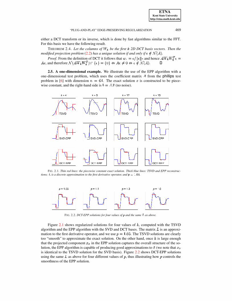
2.5. A one-dimensional example. We illustrate the use of the EPP algorithm with aone-dimensional test problem, which uses the coefficient matrix

�from the phillips test

problem in [6] with dimension � �ÌËyÍ. The exact solution

� is constructed to be piece-wise constant, and the right-hand side is

��w� (no noise).

FIG. 2.1. Thin red lines: the piecewise constant exact solution. Thick blue lines: TSVD and EPP reconstruc-tions; Î is a discrete approximation to the first derivative operator, and �2Ï�Ð±Ñ Ò±Ó .

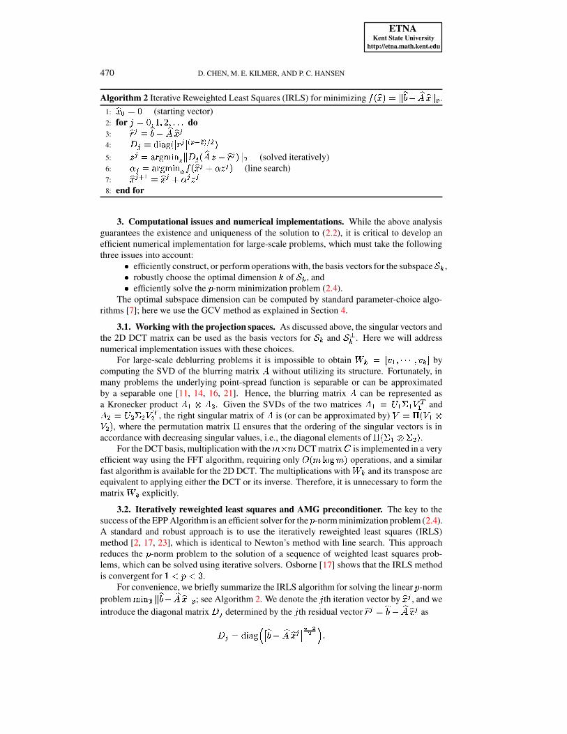
FIG. 2.2. DCT-EPP solutions for four values of � and the same Î as above.

Figure 2.1 shows regularized solutions for four values of - , computed with the TSVDalgorithm and the EPP algorithm with the SVD and DCT bases. The matrix / is an approxi-mation to the first derivative operator, and we use 5 � 6 s OuÔ . The TSVD solutions are clearlytoo “smooth” to approximate the exact solution. On the other hand, once - is large enoughthat the projected component � + in the EPP solution captures the overall structure of the so-lution, the EPP algorithm is capable of producing good approximations to

� (we note that � +is identical to the TSVD solution for the SVD basis). Figure 2.2 shows DCT-EPP solutionsusing the same / as above for four different values of 5 , thus illustrating how 5 controls thesmoothness of the EPP solution.




Algorithm 2 Iterative Reweighted Least Squares (IRLS) for minimizing Õi�cÖ� � � 0 Ö � > Ö� Ö� 0 4 .1: Ö� k � O (starting vector)2: for Ä � O H 6 H : H sPs$s do3: Ö × µ � Ö � > Ö� Ö� µ4: Ø µ2�9ÙÇ}Úv�z �{Û × µ Û Y 4 ! � ]cÜ � �5:

� µ �9v�x`zy|�}\~�� 0$Ø µ � Ö� � >gÖ× µ � 0 � (solved iteratively)6: Ý µ �wv�x`zy|�}\~®Þ Õi�cÖ� µ Ý � µ � (line search)7: Ö� µ ° " � Ö� µ Ý µ � µ8: end for

3. Computational issues and numerical implementations. While the above analysisguarantees the existence and uniqueness of the solution to (2.2), it is critical to develop anefficient numerical implementation for large-scale problems, which must take the followingthree issues into account:¡ efficiently construct, or perform operations with, the basis vectors for the subspace *Ã+ ,¡ robustly choose the optimal dimension - of *i+ , and¡ efficiently solve the 5 -norm minimization problem (2.4).

The optimal subspace dimension can be computed by standard parameter-choice algo-rithms [7]; here we use the GCV method as explained in Section 4.

3.1. Working with the projection spaces. As discussed above, the singular vectors andthe 2D DCT matrix can be used as the basis vectors for *i+ and * m+ . Here we will addressnumerical implementation issues with these choices.

For large-scale deblurring problems it is impossible to obtain fE+ �ß¢ ¤ " H 1$1P1 H ¤ + ¥ bycomputing the SVD of the blurring matrix

�without utilizing its structure. Fortunately, in

many problems the underlying point-spread function is separable or can be approximatedby a separable one [11, 14, 16, 21]. Hence, the blurring matrix

�can be represented as

a Kronecker product� "�C � � . Given the SVDs of the two matrices

� " �áà "eâ�"Pã p" and� � �bà � â � ã p� , the right singular matrix of�

is (or can be approximated by) ã ��ä � ã#" Cã � � , where the permutation matrixä

ensures that the ordering of the singular vectors is inaccordance with decreasing singular values, i.e., the diagonal elements of

ä � â " C?â � � .For the DCT basis, multiplication with the ��Ã� DCT matrix ³ is implemented in a very

efficient way using the FFT algorithm, requiring only å��=��æ ¿ z � � operations, and a similarfast algorithm is available for the 2D DCT. The multiplications with f + and its transpose areequivalent to applying either the DCT or its inverse. Therefore, it is unnecessary to form thematrix fg+ explicitly.

3.2. Iteratively reweighted least squares and AMG preconditioner. The key to thesuccess of the EPP Algorithm is an efficient solver for the 5 -norm minimization problem (2.4).A standard and robust approach is to use the iteratively reweighted least squares (IRLS)method [2, 17, 23], which is identical to Newton’s method with line search. This approachreduces the 5 -norm problem to the solution of a sequence of weighted least squares prob-lems, which can be solved using iterative solvers. Osborne [17] shows that the IRLS methodis convergent for 6N7l5�7�Ô .

For convenience, we briefly summarize the IRLS algorithm for solving the linear 5 -normproblem

|�}�~�ç� 0 Ö � > Ö� Ö� 0 4 ; see Algorithm 2. We denote the Ä th iteration vector by Ö� µ , and weintroduce the diagonal matrix Ø µ determined by the Ä th residual vector Ö× µ � Ö � > Ö� Ö� µ asØ µF��Ù�}\vyz,À®èè Ö � > Ö� Ö� µ èè=éeêyëë Â s




The Newton search direction� µ

is identical to the solution of the weighted least squaresproblem

(3.1)|�}�~� 0eØ µ®ì Ö� � >gÖ× µ ��íí � s

For 6�7�597î: , as the iteration vector Ö� µ gets close to the solution, the diagonal elementsin Ø µ increase to infinity, and this tendency increases as 5 approaches 1. Hence, the matrixØ µ Ö� in (3.1) becomes increasingly ill-conditioned as the iterations converge. It is thereforedifficult to find a suitable preconditioner for the least squares problem (3.1).

Consider the corresponding normal equationsÖ� pjØ �µ Ö� � µ � Ö� pïØ �µ Ö× µ � Ö� pïØ �µ � Ö � > Ö� Ö� µ � Hand define the new variable ð µ � � µ Ö� µ . The normal equations can then be rewritten as

(3.2) Ö� pjØ �µ Ö� ð µ � Ö� pjØ �µ Ö � sThe benefit of the above transformation is that the right-hand side in the new system (3.2)depends on iteration Ä only through Ø µ , which is known in the Ä th iteration.2

For our algorithm, it follows from (2.4) that Ö�¼� / f k and Ö �ñ� >2/ f + t + , so (3.2) canbe rewritten as

(3.3) f pk �c/ p Ø �µ / � f k ð µ � >�f pk �c/ p Ø �µ / � f + t + sSince the condition number increases as the IRLS algorithm converges to the solution, pre-conditioning is necessary when solving (3.3). Recall that / is a gradient operator, and hence/ p ØÊ�µ / represents a diffusion operator with large discontinuities in the diffusion coefficients.Algebraic multi-grid (AMG) methods are robust when the diffusion coefficients are discon-tinuous and vary widely [18, 20]. Therefore, we employ an AMG method to develop a rightpreconditioner ò for (3.3). The right-preconditioned problem is

(3.4)¢ f pk ��/ p Ø �µ / � f k ò ¥ �ð µ � >�f pk ��/ p Ø �µ / � f + t + H

where ð µ � ò �ð µ . In our implementation, given a vector¤

, the matrix-vector multiplicationÆ � ò ¤is implemented in three steps:

1. Compute �¤�� f k ¤ .2. Use the AMG method to solve �c/ p ØÊ�µ / �^ó � �¤ for

ó.

3. Compute the result Æ � f pk ó .The matrix f pk �c/ p Øô�µ / � f k is symmetric positive definite if Øô�µ is positive definite. If

not, positive definiteness of Ø��µ can be guaranteed by adding a small positive number to thediagonal elements. A first thought may be to solve (3.4) with the conjugate gradient (CG)method; but this requires that the preconditioner ò is also symmetric and positive definite.In our implementation we use the Gauss-Seidel method in the pre- and post-relaxations of theAMG method, and hence the AMG residual reduction operator is not symmetric [18], andconsequently the preconditioner is not symmetric. Instead we solve (3.1) with the GMRESalgorithm with right AMG preconditioning [19].

2We thank Eric de Sturler for pointing this out.




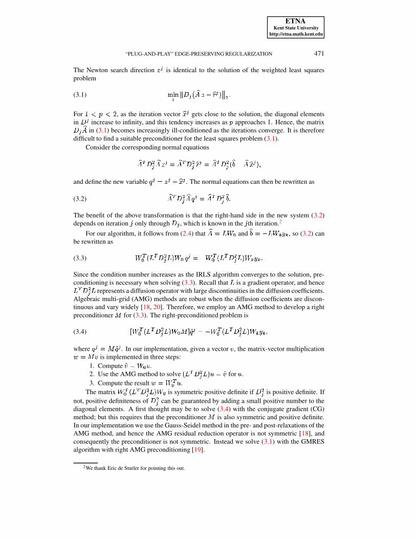
FIG. 4.1. Gaussian PSF with õFÏ8ö (left) and out-of-focus PSF with ÷ÃÏ�ö (right).

4. Numerical results. We present numerical experiments using the EPP algorithm, andwe perform a brief comparison with Total Variation deblurring. To better visualize the impactof the high-frequency correction we use Matlab’s colormap Hot for the first example, whichvaries smoothly from black through shades of red, orange, and yellow, to white, as the inten-sity increases. Throughout we use the :uø Ë �ô:uø Ë “cameraman” test image. All the numericalsimulations are performed using Matlab R2009b on a Windows 7 x86 32-bit system. The Ccompiler used to build the AMG preconditioner MEX-files is Microsoft Visual Studio 2008.

4.1. Image quality, PSFs, and algorithm parameters. The “noise level” of a test im-age is defined as 0 � 0 � ¨�0 � 0 � . The quality of the restored images is measured by the relativeerror 0 � restored > � 0 � ¨�0 � 0 � and by the MSSIM [22] (for which a larger value is better). Inour experiments the test images are generated with two common types of PSFs, Gaussianblur and out-of-focus blur, and we use reflexive boundary conditions in the restorations. Theelements of the Gaussian PSF are5 §¶µñ��ª$ù3Fú >Êû �: À ��½ï>o- � � � Ä >�ü � � Â¯ý Hand the elements of the out-of-focus PSF are5 §þµF� ÿ " ¨ Á � ë if ��½ï>o- � � � Ä > � � �� × �O otherwise Hwhere �c- H ü � is the center of the PSF, and û and × are parameters that determine the amount ofblurring; see Fig. 4.1. Both are doubly symmetric, but the latter is not separable, and thereforeit is not possible to efficiently compute the exact SVD of the corresponding matrix

�.

To compute the subspace dimension - we use the GCV method [7], which can be imple-mented very efficiently when the singular vectors or the DCT basis are used. Other methodscould also be considered (and may work well in other applications), but here we choose theGCV method for its simplicity and convenience. In this method we minimize the GCV func-tion given by

� �c- � �� h§� +±° "� �§�=�8>o- � � H for - � 6 H : H 1$1P1 H �@>?6 Hwhere § � Æ p§ � ( Æ § being either the left singular vectors

ó §or the DCT basis vectors). As

noted in [4] the GCV method very often provides a parameter that is too large, which is un-desirable in our algorithm where it is important that � + captures only the smooth componentof the solution. Also, in some of our experiments the singular vectors are approximated bya Kronecker product, which might be not accurate. Hence, to ensure that � + is smooth, we




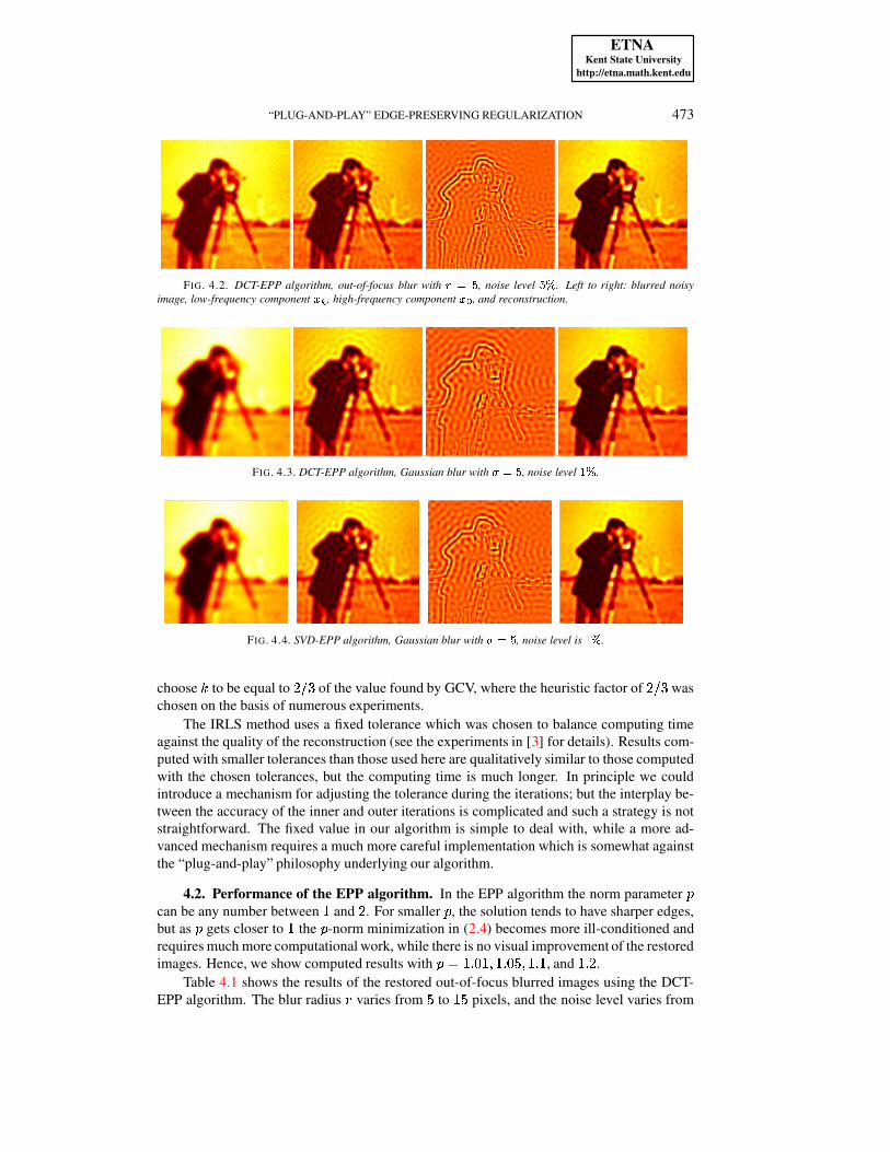
FIG. 4.2. DCT-EPP algorithm, out-of-focus blur with ÷�Ï�ö , noise level ö � . Left to right: blurred noisyimage, low-frequency component �� , high-frequency component �� , and reconstruction.

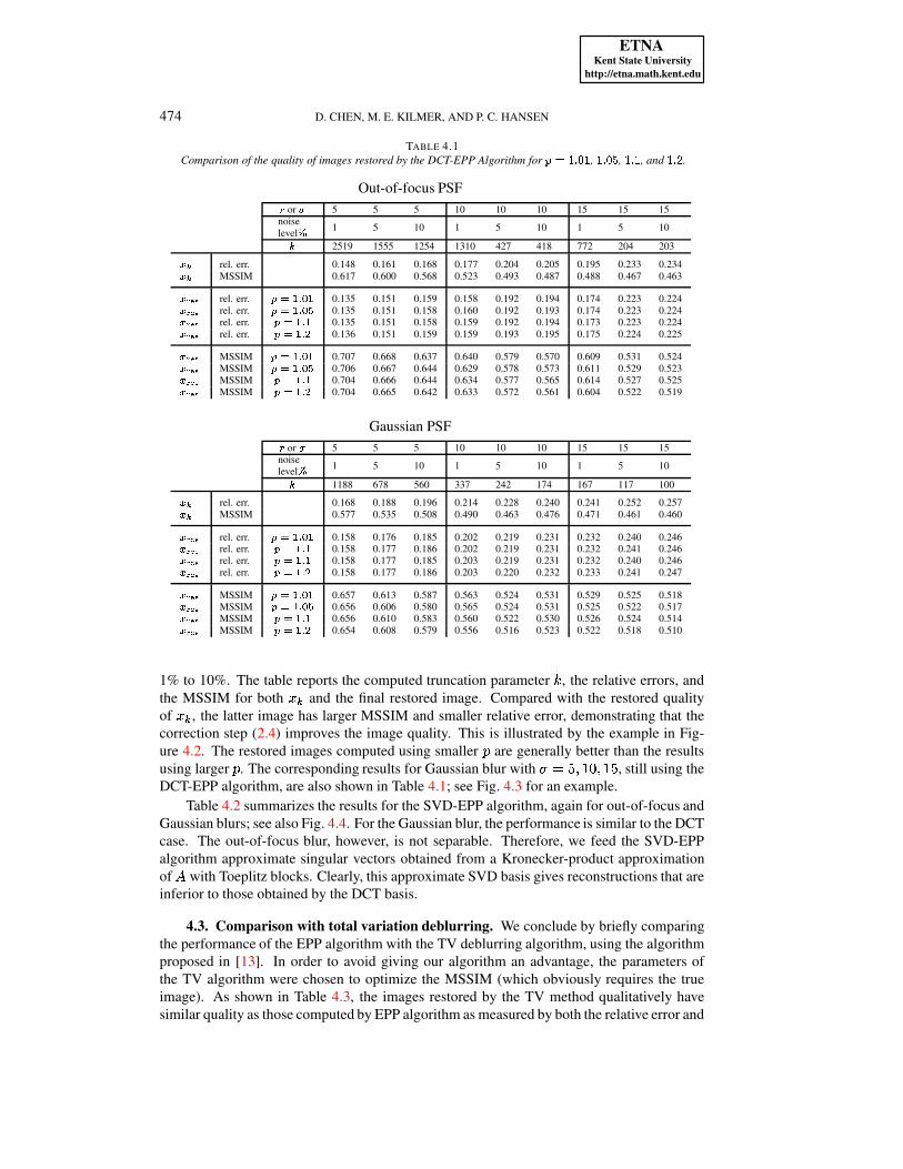
FIG. 4.3. DCT-EPP algorithm, Gaussian blur with õIÏ�ö , noise level Ð�� .

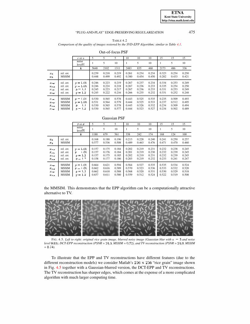
FIG. 4.4. SVD-EPP algorithm, Gaussian blur with õñÏ@ö , noise level is Ð�� .

choose - to be equal to :u¨�Ô of the value found by GCV, where the heuristic factor of :u¨<Ô waschosen on the basis of numerous experiments.

The IRLS method uses a fixed tolerance which was chosen to balance computing timeagainst the quality of the reconstruction (see the experiments in [3] for details). Results com-puted with smaller tolerances than those used here are qualitatively similar to those computedwith the chosen tolerances, but the computing time is much longer. In principle we couldintroduce a mechanism for adjusting the tolerance during the iterations; but the interplay be-tween the accuracy of the inner and outer iterations is complicated and such a strategy is notstraightforward. The fixed value in our algorithm is simple to deal with, while a more ad-vanced mechanism requires a much more careful implementation which is somewhat againstthe “plug-and-play” philosophy underlying our algorithm.

4.2. Performance of the EPP algorithm. In the EPP algorithm the norm parameter 5can be any number between 6 and : . For smaller 5 , the solution tends to have sharper edges,but as 5 gets closer to 6 the 5 -norm minimization in (2.4) becomes more ill-conditioned andrequires much more computational work, while there is no visual improvement of the restoredimages. Hence, we show computed results with 5 � 6 s O�6 H 6 s O�ø H 6 s 6 , and 6 s : .

Table 4.1 shows the results of the restored out-of-focus blurred images using the DCT-EPP algorithm. The blur radius × varies from ø to 6�ø pixels, and the noise level varies from




TABLE 4.1Comparison of the quality of images restored by the DCT-EPP Algorithm for �2ÏlÐ±Ñ Ò¦Ð , Ð±Ñ Ò±ö , Ð±ÑþÐ , and Ð±Ñ � .

Out-of-focus PSF� or � 5 5 5 10 10 10 15 15 15noiselevel � 1 5 10 1 5 10 1 5 10+ 2519 1555 1254 1310 427 418 772 204 203�� rel. err. 0.148 0.161 0.168 0.177 0.204 0.205 0.195 0.233 0.234�� MSSIM 0.617 0.600 0.568 0.523 0.493 0.487 0.488 0.467 0.463�� rel. err. 4 � " � k " 0.135 0.151 0.159 0.158 0.192 0.194 0.174 0.223 0.224� �� rel. err. 4 � " � k"! 0.135 0.151 0.158 0.160 0.192 0.193 0.174 0.223 0.224� �� rel. err. 4 � "#� " 0.135 0.151 0.158 0.159 0.192 0.194 0.173 0.223 0.224�� rel. err. 4 � "#� � 0.136 0.151 0.159 0.159 0.193 0.195 0.175 0.224 0.225� �� MSSIM 4 � " � k " 0.707 0.668 0.637 0.640 0.579 0.570 0.609 0.531 0.524�� MSSIM 4 � " � k"! 0.706 0.667 0.644 0.629 0.578 0.573 0.611 0.529 0.523�� MSSIM 4 � "#� " 0.704 0.666 0.644 0.634 0.577 0.565 0.614 0.527 0.525� �� MSSIM 4 � "#� � 0.704 0.665 0.642 0.633 0.572 0.561 0.604 0.522 0.519

Gaussian PSF� or � 5 5 5 10 10 10 15 15 15noiselevel � 1 5 10 1 5 10 1 5 10+ 1188 678 560 337 242 174 167 117 100�� rel. err. 0.168 0.188 0.196 0.214 0.228 0.240 0.241 0.252 0.257�� MSSIM 0.577 0.535 0.508 0.490 0.463 0.476 0.471 0.461 0.460�� rel. err. 4 � " � k " 0.158 0.176 0.185 0.202 0.219 0.231 0.232 0.240 0.246� �� rel. err. 4 � "#� " 0.158 0.177 0.186 0.202 0.219 0.231 0.232 0.241 0.246� �� rel. err. 4 � "#� " 0.158 0.177 0.185 0.203 0.219 0.231 0.232 0.240 0.246�� rel. err. 4 � "#� � 0.158 0.177 0.186 0.203 0.220 0.232 0.233 0.241 0.247� �� MSSIM 4 � " � k " 0.657 0.613 0.587 0.563 0.524 0.531 0.529 0.525 0.518�� MSSIM 4 � " � k"! 0.656 0.606 0.580 0.565 0.524 0.531 0.525 0.522 0.517�� MSSIM 4 � "#� " 0.656 0.610 0.583 0.560 0.522 0.530 0.526 0.524 0.514� �� MSSIM 4 � "#� � 0.654 0.608 0.579 0.556 0.516 0.523 0.522 0.518 0.510

1% to 10%. The table reports the computed truncation parameter - , the relative errors, andthe MSSIM for both � + and the final restored image. Compared with the restored qualityof � + , the latter image has larger MSSIM and smaller relative error, demonstrating that thecorrection step (2.4) improves the image quality. This is illustrated by the example in Fig-ure 4.2. The restored images computed using smaller 5 are generally better than the resultsusing larger 5 . The corresponding results for Gaussian blur with û � ø H 6PO H 6�ø , still using theDCT-EPP algorithm, are also shown in Table 4.1; see Fig. 4.3 for an example.

Table 4.2 summarizes the results for the SVD-EPP algorithm, again for out-of-focus andGaussian blurs; see also Fig. 4.4. For the Gaussian blur, the performance is similar to the DCTcase. The out-of-focus blur, however, is not separable. Therefore, we feed the SVD-EPPalgorithm approximate singular vectors obtained from a Kronecker-product approximationof�

with Toeplitz blocks. Clearly, this approximate SVD basis gives reconstructions that areinferior to those obtained by the DCT basis.

4.3. Comparison with total variation deblurring. We conclude by briefly comparingthe performance of the EPP algorithm with the TV deblurring algorithm, using the algorithmproposed in [13]. In order to avoid giving our algorithm an advantage, the parameters ofthe TV algorithm were chosen to optimize the MSSIM (which obviously requires the trueimage). As shown in Table 4.3, the images restored by the TV method qualitatively havesimilar quality as those computed by EPP algorithm as measured by both the relative error and




TABLE 4.2Comparison of the quality of images restored by the SVD-EPP Algorithm; similar to Table 4.1.

Out-of-focus PSF� or � 5 5 5 10 10 10 15 15 15noiselevel � 1 5 10 1 5 10 1 5 10+ 5648 2102 1311 2483 835 468 2173 486 336�$� rel. err. 0.239 0.218 0.219 0.261 0.234 0.234 0.323 0.254 0.250�$� MSSIM 0.448 0.499 0.492 0.380 0.454 0.450 0.202 0.433 0.421��%�� rel. err. 4 � " � k " 0.246 0.223 0.219 0.267 0.237 0.234 0.334 0.253 0.249� �%�� rel. err. 4 � " � k"! 0.246 0.224 0.218 0.267 0.236 0.233 0.335 0.254 0.250� �%�� rel. err. 4 � " � " 0.245 0.223 0.217 0.267 0.236 0.233 0.331 0.253 0.249��%�� rel. err. 4 � " � � 0.245 0.222 0.216 0.266 0.235 0.232 0.331 0.252 0.248� �%�� MSSIM 4 � " � k " 0.530 0.565 0.578 0.443 0.525 0.535 0.235 0.509 0.493��%�� MSSIM 4 � " � k"! 0.531 0.564 0.579 0.444 0.525 0.533 0.237 0.512 0.495��%�� MSSIM 4 � " � " 0.530 0.565 0.578 0.445 0.526 0.532 0.234 0.509 0.494� �%�� MSSIM 4 � " � � 0.530 0.565 0.577 0.444 0.523 0.527 0.234 0.502 0.489

Gaussian PSF� or � 5 5 5 10 10 10 15 15 15noiselevel � 1 5 10 1 5 10 1 5 10+ 1188 679 561 338 242 174 168 124 100�$� rel. err. 0.168 0.188 0.196 0.213 0.228 0.240 0.241 0.250 0.257�$� MSSIM 0.577 0.536 0.508 0.489 0.463 0.476 0.471 0.470 0.460��%�� rel. err. 4 � " � k " 0.157 0.175 0.184 0.202 0.219 0.231 0.232 0.238 0.245� �%�� rel. err. 4 � " � k"! 0.157 0.176 0.184 0.201 0.219 0.230 0.232 0.239 0.245� �%�� rel. err. 4 � " � " 0.157 0.175 0.185 0.202 0.219 0.231 0.232 0.239 0.245��%�� rel. err. 4 � " � � 0.158 0.177 0.186 0.203 0.219 0.232 0.233 0.241 0.247� �%�� MSSIM 4 � " � k " 0.664 0.621 0.594 0.564 0.527 0.535 0.535 0.534 0.524��%�� MSSIM 4 � " � k"! 0.662 0.616 0.589 0.570 0.523 0.536 0.533 0.532 0.520��%�� MSSIM 4 � " � " 0.662 0.618 0.588 0.568 0.520 0.531 0.530 0.529 0.518� �%�� MSSIM 4 � " � � 0.657 0.611 0.580 0.559 0.512 0.524 0.522 0.519 0.508

the MMSIM. This demonstrates that the EPP algorithm can be a computationally attractivealternative to TV.

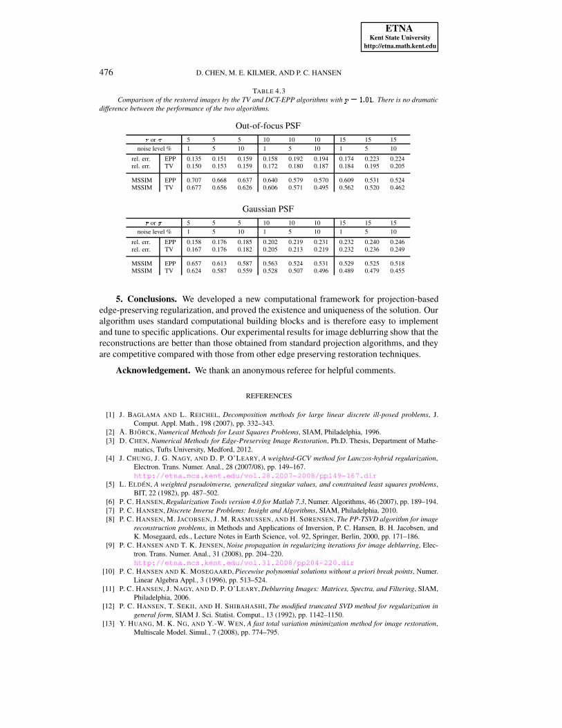
FIG. 4.5. Left to right: original rice grain image, blurred noisy image (Gaussian blur with õ�Ï�Ó and noiselevel Ò¦Ñ Ò±Ó ), DCT-EPP reconstruction (PSNR = �#&�Ñ Ó , MSSIM = Ò¦Ñ '#� ), and TV reconstruction (PSNR = �#&�Ñ ( , MSSIM= Ò¦Ñ '"& ).

To illustrate that the EPP and TV reconstructions have different features (due to thedifferent reconstruction models) we consider Matlab’s :yø Ë ��:uø Ë “rice grain” image shownin Fig. 4.5 together with a Gaussian-blurred version, the DCT-EPP and TV reconstructions.The TV reconstruction has sharper edges, which comes at the expense of a more complicatedalgorithm with much larger computing time.




TABLE 4.3Comparison of the restored images by the TV and DCT-EPP algorithms with ��Ï�Ð±Ñ Ò¦Ð . There is no dramatic

difference between the performance of the two algorithms.

Out-of-focus PSF� or � 5 5 5 10 10 10 15 15 15noise level % 1 5 10 1 5 10 1 5 10

rel. err. EPP 0.135 0.151 0.159 0.158 0.192 0.194 0.174 0.223 0.224rel. err. TV 0.150 0.153 0.159 0.172 0.180 0.187 0.184 0.195 0.205

MSSIM EPP 0.707 0.668 0.637 0.640 0.579 0.570 0.609 0.531 0.524MSSIM TV 0.677 0.656 0.626 0.606 0.571 0.495 0.562 0.520 0.462

Gaussian PSF� or � 5 5 5 10 10 10 15 15 15noise level % 1 5 10 1 5 10 1 5 10

rel. err. EPP 0.158 0.176 0.185 0.202 0.219 0.231 0.232 0.240 0.246rel. err. TV 0.167 0.176 0.182 0.205 0.213 0.219 0.232 0.236 0.249

MSSIM EPP 0.657 0.613 0.587 0.563 0.524 0.531 0.529 0.525 0.518MSSIM TV 0.624 0.587 0.559 0.528 0.507 0.496 0.489 0.479 0.455

5. Conclusions. We developed a new computational framework for projection-basededge-preserving regularization, and proved the existence and uniqueness of the solution. Ouralgorithm uses standard computational building blocks and is therefore easy to implementand tune to specific applications. Our experimental results for image deblurring show that thereconstructions are better than those obtained from standard projection algorithms, and theyare competitive compared with those from other edge preserving restoration techniques.

Acknowledgement. We thank an anonymous referee for helpful comments.

REFERENCES

[1] J. BAGLAMA AND L. REICHEL, Decomposition methods for large linear discrete ill-posed problems, J.Comput. Appl. Math., 198 (2007), pp. 332–343.

[2] A. BJORCK, Numerical Methods for Least Squares Problems, SIAM, Philadelphia, 1996.[3] D. CHEN, Numerical Methods for Edge-Preserving Image Restoration, Ph.D. Thesis, Department of Mathe-

matics, Tufts University, Medford, 2012.[4] J. CHUNG, J. G. NAGY, AND D. P. O’LEARY, A weighted-GCV method for Lanczos-hybrid regularization,

Electron. Trans. Numer. Anal., 28 (2007/08), pp. 149–167.http://etna.mcs.kent.edu/vol.28.2007-2008/pp149-167.dir

[5] L. ELDEN, A weighted pseudoinverse, generalized singular values, and constrained least squares problems,BIT, 22 (1982), pp. 487–502.

[6] P. C. HANSEN, Regularization Tools version 4.0 for Matlab 7.3, Numer. Algorithms, 46 (2007), pp. 189–194.[7] P. C. HANSEN, Discrete Inverse Problems: Insight and Algorithms, SIAM, Philadelphia, 2010.[8] P. C. HANSEN, M. JACOBSEN, J. M. RASMUSSEN, AND H. SØRENSEN, The PP-TSVD algorithm for image

reconstruction problems, in Methods and Applications of Inversion, P. C. Hansen, B. H. Jacobsen, andK. Mosegaard, eds., Lecture Notes in Earth Science, vol. 92, Springer, Berlin, 2000, pp. 171–186.

[9] P. C. HANSEN AND T. K. JENSEN, Noise propagation in regularizing iterations for image deblurring, Elec-tron. Trans. Numer. Anal., 31 (2008), pp. 204–220.http://etna.mcs.kent.edu/vol.31.2008/pp204-220.dir

[10] P. C. HANSEN AND K. MOSEGAARD, Piecewise polynomial solutions without a priori break points, Numer.Linear Algebra Appl., 3 (1996), pp. 513–524.

[11] P. C. HANSEN, J. NAGY, AND D. P. O’LEARY, Deblurring Images: Matrices, Spectra, and Filtering, SIAM,Philadelphia, 2006.

[12] P. C. HANSEN, T. SEKII, AND H. SHIBAHASHI, The modified truncated SVD method for regularization ingeneral form, SIAM J. Sci. Statist. Comput., 13 (1992), pp. 1142–1150.

[13] Y. HUANG, M. K. NG, AND Y.-W. WEN, A fast total variation minimization method for image restoration,Multiscale Model. Simul., 7 (2008), pp. 774–795.

http://etna.mcs.kent.edu/vol.28.2007-2008/pp149-167.dir

http://etna.mcs.kent.edu/vol.31.2008/pp204-220.dir




[14] J. KAMM AND J. G. NAGY, Optimal Kronecker product approximation of block Toeplitz matrices, SIAM J.Matrix Anal. Appl., 22 (2000), pp. 155–172.

[15] J. L. MUELLER AND S. SILTANEN, Linear and Nonlinear Inverse Problems with Practical Applications,SIAM, Philadelphia, 2012.

[16] J. G. NAGY, M. K. NG, AND L. PERRONE, Kronecker product approximations for image restoration withreflexive boundary conditions, SIAM J. Matrix Anal. Appl., 25 (2003), pp. 829–841.

[17] M. R. OSBORNE, Finite Algorithms in Optimization and Data Analysis, Wiley, Chichester, 1985.[18] J. W. RUGE AND K. STUBEN, Algebraic multigrid, in Multigrid Methods, S. McCormick, ed., Frontiers

Appl. Math., vol. 3, SIAM, Philadelphia, 1987, pp. 73–130.[19] Y. SAAD AND M. H. SCHULTZ, GMRES: a generalized minimal residual algorithm for solving nonsymmetric

linear systems, SIAM J. Sci. Statist. Comput., 7 (1986), pp. 856–869.[20] U. TROTTENBERG, C. W. OOSTERLEE, AND A. SCHULLER, Multigrid, Academic Press, San Diego, 2001.[21] C. F. VAN LOAN AND N. PITSIANIS, Approximation with Kronecker products, in Linear Algebra for Large

Scale and Real-time Applications, M. S. Moonen, G. J. Golub, B. L. R. De Moor, eds., vol. 232 of NATOAdv. Sci. Inst. Ser. E Appl. Sci., Kluwer, Dordrecht, 1993, pp. 293–314.

[22] Z. WANG, A. BOVIK, H. SHEIKH, AND E. SIMONCELLI, Image quality assessment: from error visibility tostructural similarity, IEEE Trans. Image Process., 13 (2004), pp. 600–612.

[23] R. WOLKE AND H. SCHWETLICK, Iteratively reweighted least squares: algorithms, convergence analysis,and numerical comparisons, SIAM J. Sci. Statist. Comput., 9 (1988), pp. 907–921.

ﬁplug-and-playﬂ edge-preserving...

Documents