C 134571

STIFF SYSTEHS OF ORDINK~jy DFBET

CU (C722

PL:L OtisLTO

https://ntrs.nasa.gov/search.jsp?R=19740020609 2018-06-22T17:21:08+00:00Z

CR 134571

Technical Report No. W /*dNumerical Solution of Stiff Systems

of Ordinary Differential Equations

with Applications to Electronic Circuits

Jerrold Stephen Rosenbaum

1971

Vincent R. LalliProject ManagerLewis Research CenterOffice of Reliability& Quality Assurance21000 Brookpark RdCleveland, OH 44135

This research was partially supported by the National

Science Foundation under grant GK - 2283 and the National

Aeronautics and Space Administration under grant NGR 33-008-090.

ABSTRACT

Numerical Solution of Stiff Systems of Ordinary Differential

Equations with Applications to Electronic Circuits

Jerrold S. Rosenbaum

Systems of ordinary differential equations inwhich the

magnitudes of the eigenvalues (or time constants) vary greatly

are commonly called stiff. Such systems of equations arise

in nuclear reactor kinetics, the flow of chemically reacting

gas, dynamics, control theory, circuit analysis and other

fields.

It is often the case that the solution is smooth outside

one or more almost-discontinuous segments. However, during

an almost-discontinuous segment, there is a rapid (sometimes

almost-discontinuous) variation in the solution.

The research reported herein develops a new A-stable

numerical integration technique for solving stiff systems of

ordinary differential equations. The method, which.is called

the generalized trapezoidal rule, is a modification of the

trapezoidal rule. However, the new method is computationally

more efficient than the trapezoidal rule when the solution of

the almost-discontinuous segments is being calculated.

The basic aim of the new numerical integration technique

is to transform the original system of differential equations

to a new system of equations such that the eigenvalues of

i

the transformed system are smaller in magnitude than the

eigenvalues of the original system. Also, the ratio of the

real parts of the largest to the smallest eigenvalue of the

transformed system is smaller than the same ratio for the

original system. A consequence of shifting the eigenvalues

is that for the same accuracy, one can integrate the new

system of equations with a larger time step than is possible

for the original system.

Particular attention has been focused on numerically

integrating the differential equations for a high frequency

model of a semiconductor network. It is shown how the

generalized trapexoidal rule can be used to integrate the

circuit equations more efficiently than the trapezoidal rule.

Also, because one has an a priori knowledge of the structure

of the circuit equations and the nature of their solution,

one can obtain additional computational economies when

integrating the circuit equations be the generalized trapezoidal

rule.

In the appendix, there is a computer program for the

generalized trapexoidal rule written in PL/I.

ii

ACKNOWLEDGEMENTS

The author wishes to express his sincere gratitude to

Professor Thomas E. Stern for his valuable guidance and en-

couragement during the course of this research.

The aughor also wishes to express his gratitude to Professor

Henry E. Meadows for his valuable guidance and inspiration

during the absence of Professor T. E. Stern.

The author wishes to thank his wife, Eileen, for her patience

during the course of the research, and for her typing.

This research was partially supported by the National

Science Foundation under grant GK - 2283 and the National

Aeronautics and Space Administration under grant NGR 33-008-009.

111

Table of Contents

I. Introduction 1

II. General Problem of Stiff Systems (Background)1. Stability 52. A-stability 113. Generalized Runge-Kutta Processes 144. Implicit Runge-Kutta Processes 175. Trapezoidal Rule, Backwards Euler

and Implicit Midpoint Methods 186. Exponential Fitting 217. Global Extrapolation 248. Alternatives to A-stability 27

III. Generalized Trapezoidal Rule1. Description of the Integration Scheme 31

a. Calculation of the Smooth Segments 33b. Calculation of the Almost-

Discontinuous Segments 362. Rationale of the Integration Scheme 433. Theoretical Error Calculations 46

a. Theoretical Errors for Various Systemsof Ordinary Differential Equations 47

b. Accuracy of the Pade Approximations 534. Step Size Control and Detection of the

Almost-Discontinuous Segments 565. Illustrative Computer Results 58

IV. Application of the Generalized Trapezoidal Ruleto Semiconductor Networks1. Semiconductor Network Equations 642. Detection of Smooth and Almost-Discontinuous

Segments 703. Application of the Generalized Trapezoidal

Rule to an Astable Multivibrator Circuit 72

V. Conclusions and Suggestions for Further Research1. Conclusions 822. Suggestions for Further Research 85

VI. References 87

VII. Appendix (Computer Program for the GeneralizedTrapezoidal Rule) 90

I. Introduction

Systems of ordinary differential equations in which the

magnitudes of the eigenvalues (or time constants) vary

greatly are commonly called stiff. Such systems of equations

arise in nuclear reactor kinetics, the flow of chemically

reacting gas, dynamics, control theory, circuit analysis and

other fields. [1,12,14,18,20,21]

It is often the case that the solution is smooth outside

of one or more almost-discontinuous segments [21] (or transient

phases or boundary layers). However, during an almost-

discontinuous phase, there is a rapid (sometimes almost-

discontinuous) variation in the solution. In addition, the

system of differential equations is usually asymptotically

stable --i.e., all the eigenvalues of the system of equations

are in the left half plane (LHP).

A similar stiffness problem arises when a partial differ-

ential equation is approximated by a large system of ordinary

differential equations. By differencing one of the variables

(usually a space variable), the initial value problem for

the resulting system of ordinary differential equations

generally has a wide spread in time constants ( see section

II.I).

Numbers in brackets indicate references listed in Chapter VI.

2

For most numerical integration schemes, in order to

prevent the numerical solution from becoming unstable, the

maximum step size that can be used to integrate a system

of equations is on the order of the smallest time constant

of the system. The step size limitation necessitates taking

an excessively large number of steps to obtain the solution

in both the smooth and almost discontinuous segments. In

particular, during the smooth regions, one would like to use

step sizes that are on the order of the largest time constant

since the local variation is small. But, one must still take

small time steps (on the order of the smallest time constant)

to prevent the numerical solution from becoming unstable.

In the case of a semiconductor switching circuit, the

solution is slowly varying except at the switching "instants".

However, if one uses the usual integration schemes, which

are generally step length limited, the largest step size

allowable throughout the entire solution is on the order of

the switching time even though the solution may be almost

constant between switching instants.

The purpose of the research reported herein is to develop

a new numerical integration technique for stiff systems of

ordinary differential equations. The method, which will be

called the generalized trapezoidal rule, is a modification

of the trapezoidal rule. However, the new method is computation-

ally more efficient than the trapezoidal rule when the solution

of an almost-discontinuous segment is being computed.

Many different approaches have been suggested for

obtaining the numerical solution of stiff systems of ordinary

differential equations. Almost all of the suggested methods

require the solution of a system of implicit (usually non-

linear) equations at each time step. In chapter II, there

is a discussion of some of the methods used to overcome the

usual step length limitations when integrating stiff systems.

In addition, there is a brief discussion of methods for solv-

ing the implicit equations that are generated by the various

integration schemes. We also attempt to show how the integration

methods are interrelated.

Chapter III is concerned with a new method for numerical

integration of stiff systems of ordinary differential equations.

The method is a modification of the trapezoidal rule. The

basic approach of the method is: (1) to modify the given

differential equations so that they are less stiff and

consequently "easier" to integrate; and (2) to use differing

approaches to obtain the numerical solution during the

almost-discontinuous and smooth sections of the solution.

The objectives of the new method are to allow the user to

take larger time steps during the almost-discontinuous

segments of the solution and to do fewer iterations per

step in order to solve the implicit integrating equations

while, at the same time, maintaining the same or improved

accuracy as compared with the trapezoidal rule.

In the research reported herein particular attention

4

has been focused on numerically integrating the differential

equations for a high frequency model of a semiconductor

network [9,18,20,21]. In Chapter IV, it is shown how the

integration method of the previous chapter can be used to

integrate the circuit equations and how, because of an a

priori knowledge of the structure of the circuit equations

and the nature of their solution, one can obtain additional

economies when integrating the circuit equations.

Chapter V presents a summary of the results of the

previous chapters and suggestions for further research.

5

II. General Problem of Stiff Systems

1. Stability

In the general theory of numerical solution of ordinary

differential equations, a major concern is the stability of

the numerical solution. Roughly speaking, the stability of

a numerical method refers to the behavior of the difference

between the actual and calculated solution as the number

of steps becomes large [14]. The values of the step size,

h, for which a particular integration method is stable, are

a function of the characteristic roots, ui , of the integration

method and the eigenvalues, Xi , of the Jacobian of the

system of ordinary differential equations being integrated

[4,10,11,12,14].

The region of the hX-plane for which all the character-

istic roots of the integration scheme are on or in the unit

circle is called the region of stability. If the stability

region is bounded, then the integration method is called

step length limited.

To demonstrate the general type of step length limitation

that can be encountered with stiff systems and the problems

that the step length limitation can cause, it is useful

to examine a linear system of ordinary differential equations:

(2.1) : = Ax, x(O) = x0

6

where the eigenvalues of A are distinct and in the LHP.

/ If the real parts of some of the eigenvalues of A

are very much larger in magnitude than the real parts of

others, the terms corresponding to the "large" eigenvalues

become negligible very quickly. This type of behavior can

also arise with nonlinear systems of equations or even

with a single equation (see section 111.3). All that is

required for a system to be stiff is that any transient

be damped out quickly in relation to the steady-state solution.

The difficulty in trying to use many of the common

numerical methods to integrate stiff equations is well

known. A numerical method can be affected by the transient

components of the solution even after the effects of those

components have become negligible in the true solution.

Analytically, this behavior of the numerical solution leads

to a restriction on the allowable step size. When many

numerical methods are applied to the linear equations (2.1),

the step size restriction takes the form:

(2.2) hil < d, i= 1,2,...,m

where h is the step size, and d is some constant which is

typically about 1 to 6. If some of the Ixbi are large,

equation (2.2) forces the numerical method to use a very

small step size in order to maintain stability, even though

the corresponding contributions to the true solution are

negligible.

7

For the linear system of equations (2.1), the analytic

solution is

nhA(2.3) x(nh) = e x o

As a consequence, any numerical procedure must, in some

hAway, approximate e hA. Also, because all the eigenvalues

of A are in the LHP, the least one should require is that

(2.4) Lim xn = 0,n a n - th

where x is the value of the solution at the n point

in the calculation.

When one applies the forward Euler, Heun or traditional

fourth-order Runge-Kutta schemes to equation (2.1), it can

be shown that

(2.5) Xn = [M(hA)] x

where

I + Z Forward Euler

(2.6) M(Z)= I + Z + Z2 /2+ Heun

I + Z + Z2 /21 + Z3 /31 + Z4 /4 . Runge-Kutta

Therefore, in order to satisfy equation (2.4), one

must require that

(2.7) IIM(hA)II<1.

Since the eigenvalues of A are distinct, there exists a

matrix P such that

(2.8) PAP -1 = diag(X1,...,) = X

Consequently, equation (2.5) can be rewritten as

8

(2.9) Xn = M(hPXP )] x0-1. = P[M (hXk) P- xo

and equation (2.7) can be reduces to

(2.10) I M(hXi) <1 for i=l,...m.

One can think of equation (2.10) as requiring that the

integration schemes be contraction operators on the left

half hX-plane (or have spectral radii less than 1).

In particular, for the forward Euler method, one has

that

(2.11) xn = x + hf(tnx 1 )

-1= P(l+hX)P xnl

Hence,

(2.12) ll+hXil<l for i = 1,...m

or, if all the eigenvalues are real,

IhXil<2

For the Heun method, the stability criterion is also

IhkX<2 and for the fourth-order Runge-Kutta method, the

criterion is Ijhx<2.78 [61.

However, one is generally interested in obtaining

the solution over the interval t = [0,q(maxlxj.-)].

If min Ixi<<maxlXjl, then stability considerations dictate

a very small step size, h =&(minl.jl-l), over the entire

interval even though the effects of the maximal eigenvalue

on the solution are negligible after the first few steps.

To demonstrate explicitly the problems caused by the

9

wide spread in the eigenvalues, two systems of ordinary

differential equations (one of which is stiff) which possess

"almost" the same solution, will be considered.

The first system is

(2.13) dVt DV+C , V() = 0, D= .- and C 2]

The solution to equations (2.13) are

V1(t) = V2(t) = 2(l-e-t )

and the stability conditions are h < 2 for the Euler and

Heun methods and h < 2.78 for the Runge-Kutta methods.

If, on the other hand, one considers the system

(2.14) dW = AW + C, W(0) = A499.5dt + C499.5 -500.

then

W(t) = 2(1-e-t )_.le - 1 0 0 0 t

W2(t) = 2(1-e-t)+0.1e -1000t

But, fbr t > 0.02, one has that 0.1e -1000le < 2.5 * 1010

or V ; W for t > 0.02. However, the eigenvalues of A are

-1 and -1000, which dictates that h < 0.002 for the Euler

and Heun methods and h < 0.00278 for the Runge-Kutta method

[6].

Now, in both systems, one wishes to determine the solution

over the interval t = [0, 6()]. For the V equations,

one would need less than 10 steps to obtain the solution

10

over the desired interval. But, for the W equations, one

woald require 1000 times as many steps to obtain the solution,

and increased precision might be needed for the calculation

because of the increased round-off error introduced by the

very large number of steps.

From the example, one can see that the step size,

h, cannot be chosen to represent the information carried

by modes corresponding to the smaller eigenvalues. The step

size must be chosen to avoid any spurious amplification of

the modes corresponding to the larger eigenvalues of the sys-

tem of equations. Thus, if an integration scheme has a bound-

ed region of stability, one is forced to take exceedingly

small time steps throughout the time interval for which

a solution is desired in order to prevent instability.

The instability is a result of an amplification of the

modes corresponding to the larger eigenvalues.

In the numerical solution of partial differential

equations, the same type'of problem is encountered when one

approximates a partial differential equation by a system

of ordinary differential equations. For example, consider

the heat equation:

(2.15) K 2u = , u(0,t) = u(L,t) = 0.

One of the standard first steps in the numerical

solution of equation (2.15) is to difference it in the

x (or space) direction. This given the following system

of ordinary differential equations:

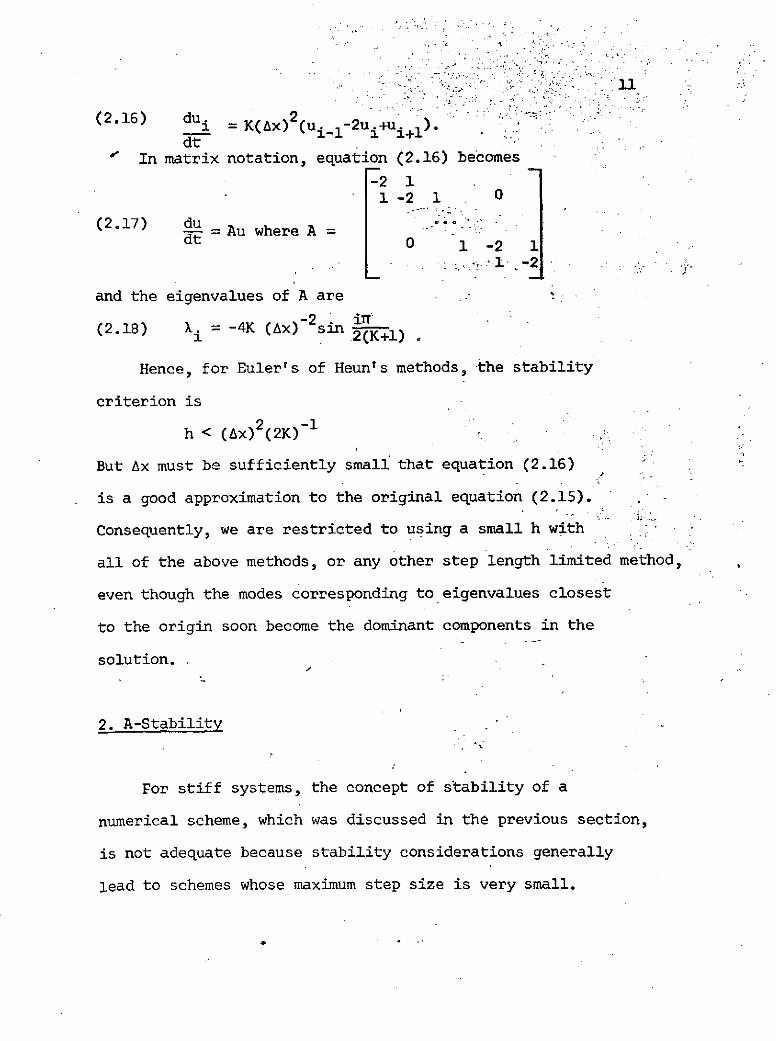
(2.16) dui = K(Ax)2 (ui _-2ui+ui+l).dt

' In matrix notation, equation (2.16) becomes

-2 11 -2 1 0

(2.17) du2. du = Au where A =dt 0 1 -2 1

and the eigenvalues of A are

-2 in(2.18) X. = -4K (Ax) sin

1 2(K+1)

Hence, for Euler's of Heun's methods, the stability

criterion is

h < (Ax)2(2K)-1

But Ax must be sufficiently small that equation (2.16)

is a good approximation to the original equation (2.15).

Consequently, we are restricted to using a small h with

all of the above methods, or any other step length limited method,

even though the modes corresponding to eigenvalues closest

to the origin soon become the dominant components in the

solution.

2. A-Stability

For stiff systems, the concept of stability of a

numerical scheme, which was discussed in the previous section,

is not adequate because stability considerations generally

lead to schemes whose maximum step size is very small.

Ideally, the step size should be a function only of the rate

otvariation of the solution during the particular interval

being calculated and the desired accuracy (rather than being

a function of the global properties of the solution).

Also, for stiff systems, it is not enough that the transient

solutions be bounded; one needs a numerical method that

insures one that all transient solutions will eventually

die out. Towards these ends, the concept of A-stability

was proposed by G. Dahlquist [3].

Definition: A numerical method for solving differential

equations is called A-stable if all solutions tend

toward zero as n- - when the method is applied with

fixed positive h to any differential equation of the

form:

* =qx

where q is a complex constant with negative real part.

In effect, the definition requires that for all eigen-

values in the LHP, the numerical solution corresponding to

those eigenvalues eventually die out regardless of the

step size. As pointed out earlier, an A-stable method

may be regarded as one which acts-as a contraction operator

for equations with eigenvalues in the LHP, although this

concept is not found in the literature on numerical integration

techniques.

The numerical integration of stiff systems has been

considered by many authors (see references). It is known

that all explicit schemes of the linear multistep and

Runge-Kutta types are step length limited and consequently

not A-stable. Therefore, attention must be focused on other

classes of integration schemes (usually implicit).

No explicit Runge-Kutta scheme is A-stable, because

the recurrence relation it produces when applied to the

test equation :c = qx is xn+1 = C(hq) xn where C(hq) is

a truncated exponential series for ehq. If q is in the

LHP, then the sequence ([x does not converge to zero for

arbitrary positive h. In fact, for almost every initial

value, x0 , xn - for almost all values of q and h.

In a paper by Ehle [6), it is shown that Butcher's

fourth-order implicit Runge-Kutta scheme is A stable; but,

the non-linear functional equations that must be solved

at each time step are considerably more complex than those

for linear multistep methods.

An indirect approach to the integration problem for

stiff systems is to transform the system of differential

equations into a new system (suitably modified) that is

not stiff and to solve the latter system by a conventional

method which is step length limited. Lawson [13] proposed

what he called a "Generalized Runge-Kutta" scheme involving

the Jacobian matrix and exponential shifts in the variables

(see section 11.3).

14

The basic theory of stiff linear multistep methods

way developed by G. Dahlquist [3]. He showed that no explicit

linear multistep method is A-stable, and'he proved the

remarkable theorem that for fixed h, the most accurate

linear multistep method is of order two, with the trapezoidal

rule having the minimum truncation error of all second

order A-stable schemes. Dahlquist also pointed out that

an iterative technique like Newton-Raphson iteration must

be used to solve the implicit integrating equations because

the method of successive substitutions is inherently step

length limited (see section 1I.5).

More recently, Widlund [24] and Gear [8] have developed

higher order multistep schemes which are, for practical

purposes, not step length limited. Widlund developed third

and fourth order schemes and Gear developed second through

sixth order schemes. But, both authors use a "milder"

form of Dahlquist's concept of A-stability. The approaches

of these two authors are discussed in section 11.7.

3. Generalized Runge-Kutta Processes [133

The basic problem inherent in all implicit integration

schemes is that one must solve a system of implicit non-

linear equations at each step. In order to avoid some of

these problems, Lawson [13] proposed to alter the stiff

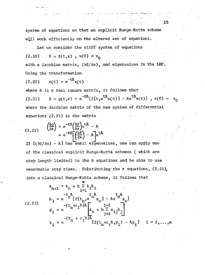
system of equations so that an explicit Runge-Kutta scheme

wll work efficiently on the altered set of equations.

Let us consider the stiff system of equations

(2.19) k = f(t,x) , x(0) = x0

with a Jacobian matrix, (.f/3x), and eigenvalues in the LHP.

Using the transformation

(2.20) z(t) = e-tA x(t)

where A is a real square matrix, it follows that

(2.21) 2 = g(t,z) = e-tA f[t,etAz(t)] - AetAz(t)} , z(0) = X

where the Jacobian matrix of the new system of differential

equations (2.21) is the matrix

(2.22) z)= e T-)- A-tA[ff N) tA

If [(3f/ax) - A] has small eigenvalues, one can apply one

of the classical explicit Runge-Kutta schemes ( which are

step length limited) to the z equations and be able to use

reasonable step sizes. Substituting the z equations, (2.21),

into a classical Runge-Kutta scheme, it follows thatm

z n+l= z n + h E bikii=l

-tA tA tAk = e n [f[t [t ,e n z] - Ae n Zn

(2.23) Pi -(t +cih)A n +h hC k

= e n i nz + h_ ai.

-(tn + c.h)Ak. = e n 1 [f(t n+c.h,p.) - APi] i= 2,...,m

1 n 1 1 1

16

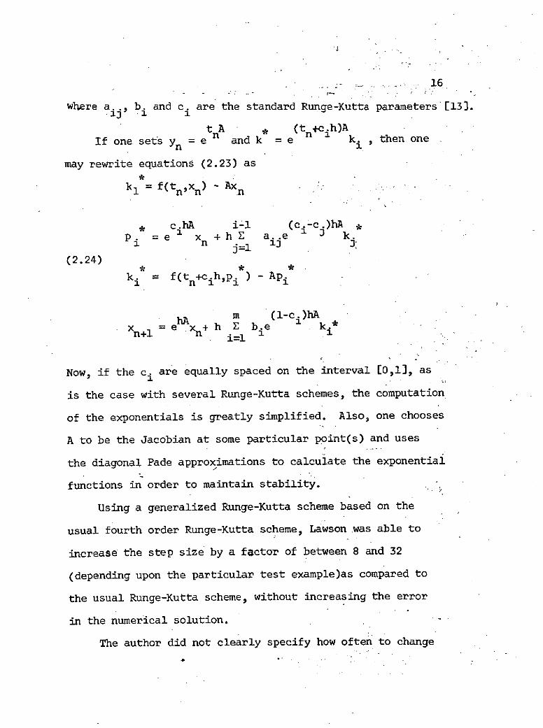
where a..i b. and c. are the standard Runge-Kutta parameters [13).

tA * (tn+cih)AIf one sets yn = e and k =e ki , then one

may rewrite equations (2.23) as

k = f(tn, n ) Axn

* c.hA i-i (c.-c.)hA kp = e Xn + h E a..e k.

j=1 3 3

(2.24)

k. = f(t +c.hp ) - Api1 n i'i

m (1-ci)hAXn+= e x+ h E be k*

n i=l

Now, if the ci are equally spaced on the interval [0,1), as

is the case with several Runge-Kutta schemes, the computation

of the exponentials is greatly simplified. Also, one chooses

A to be the Jacobian at some particular point(s) and uses

the diagonal Pade approximations to calculate the exponential

functions in order to maintain stability.

Using a generalized Runge-Kutta scheme based on the

usual fourth order Runge-Kutta scheme, Lawson was able to

increase the step size by a factor of between 8 and 32

(depending upon the particular test example)as compared to

the usual Runge-Kutta scheme, without increasing the error

in the numerical solution.

The author did not clearly specify how often to change

17

A and how to select h.

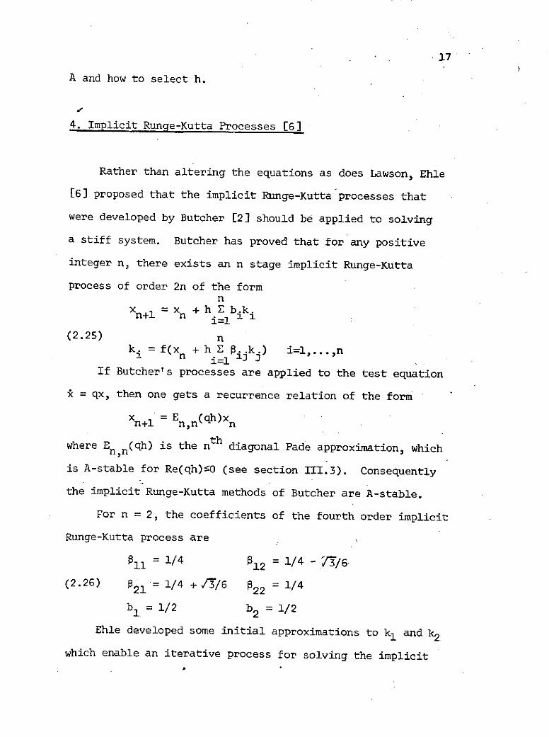
4. Implicit Runge-Kutta Processes [6]

Rather than altering the equations as does Lawson, Ehle

[6] proposed that the implicit Runge-Kutta processes that

were developed by Butcher [2] should be applied to solving

a stiff system. Butcher has proved that for any positive

integer n, there exists an n stage implicit Runge-Kutta

process of order 2n of the formn

Xn+ = x + h b.k.i=l

(2.25) nk = f(x + hi ijk) i=... n1 n _i= 1 ,.

If Butcher's processes are applied to the test equation

5 = qx, then one gets a recurrence relation of the form

Xn+l = En,n(qh)x n

where En,n(qh) is the nth diagonal Pade approximation, which

is A-stable for Re(qh)-O (see section III.3). Consequently

the implicit Runge-Kutta methods of Butcher are A-stable.

For n = 2, the coefficients of the fourth order implicit

Runge-Kutta process are

o11 = 1/4 P12 = 1/4 - 3/6

(2.26) P21 = 1/4 + /T/6 22 = 1/4

b 1 = 1/2 b2 = 1/2

Ehle developed some initial approximations to kl and k2which enable an iterative process for solving the implicit

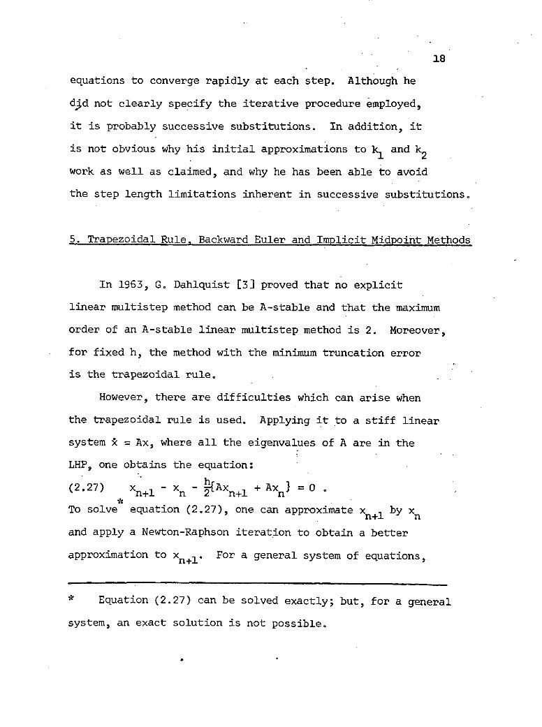
18

equations to converge rapidly at each step. Although he

djd not clearly specify the iterative procedure employed,

it is probably successive substitutions. In addition, it

is not obvious why his initial approximations to k, and k2work as well as claimed, and why he has been able to avoid

the step length limitations inherent in successive substitutions.

5. Trapezoidal Rule, Backward Euler and Implicit Midpoint Methods

In 1963, G. Dahlquist [3] proved that no explicit

linear multistep method can be A-stable and that the maximum

order of an A-stable linear multistep method is 2. Moreover,

for fixed h, the method with the minimum truncation error

is the trapezoidal rule.

However, there are difficulties which can arise when

the trapezoidal rule is used. Applying it to a stiff linear

system :k = Ax, where all the eigenvalues of A are in the

LHP, one obtains the equation:

(2.27) x+ 1 - xn - Ax + Axn =o

To solve equation (2.27), one can approximate Xn+1 by xnand apply a Newton-Raphson iteration to obtain a better

approximation to xn+l. For a general system of equations,

Equation (2.27) can be solved exactly; but, for a general

system, an exact solution is not possible.

19

the Newton-Raphson iteration is used repeatedly to get in-

creasingly better approximations to Xn+1 until two successive

approximations to Xn+1 differ by some specified small amount.

The number of iterations that is necessary for convergence

is often used to adjust the step size which, in turn, controls

the truncation error of the entire procedure.

However, in the case of a linear system, the first

iteration yields the result#

(2.28) X+ 1 = C(Ah)x where C(Ah) = I +(1/2)Ahn+ n I -(1/2)Ah

which is the exact solution to equation (2.27). Except for

rounding errors, further Newton-Raphson iterations do not

alter the value of Xn+ 1 that is given in equation (2.28).

Consequently, if one is not careful, counting the number of

iterations for the approximations to xn+1 to converge can

be very misleading when one uses the number of iterations

to control the step size.

Also, even though IIC(Ah)JII 1 for Re(k) : 0 (i.e. the

method is A-stable), as h becomes large, C(Xh) - -1. That

is, the numerical solution has a tendency towards slowly

damped oscillations which can be very troublesome during

the calculation of the transient phases of the solution.

To avoid the oscillatory problem, one can use small

# In a matrix equation, whenever a fraction of the form

N/D appears, we are using the notation to mean the matrix

D-N.

20

steps during the transient phases when rapidly changing

cemponents affect the solution. But, once the amplitude of

the transients has become sufficiently small, one can start

using larger time steps that are adjusted to the rate of

change of the solution.

A second way to cope with the oscillations for a general

equation is to use a smoothing process proposed by B. Lindberg

[15]. He suggested that one calculate the function values

at the points tn, tn+l, and tn+2O Then one setsA

(2.29) Xn+l =(1/4)(x + 2 Xn+l + Xn2 )

and continues the integration from tn+1 (that is, backtracking

Aone step) using the smoothed value, Xn+l, as the function

value.

A third way of coping with the oscillations is to use

the backwards Euler scheme. For a linear system, one obtains

the relation

(2.30) Xn+1 = C'(Ah)xn where C'(Ah) = II - Ah

which is also A-stable for systems with eigenvalues in the LHP.

However, one has that C'(Xh)- 0 as Re(Xh)- --, which is

desirable when the contributions to the solution correspons-

ing to the eigenvalues with large negative real parts is

still significant. It must be remembered that the backwards

Euler scheme is only a first order scheme and that care must

be taken because the damping factor C'(Ah) may be too strong

and consequently produce an underestimate of the exact

21

solution.

It is interesting to note that in both cases the

multiplicative quotients, C(Ah) and C'(Ah), are Pade

approximations to the exponential function [19).

H. J. Stetter [22] has pointed out that for fixed h, the

implicit midpoint method

(2.31) xn+l - xn = f(tn+ 2 ,n+ 1 2 ) where x n+/2 = Xn+l Xn

is equivalent to the trapezoidal rule. Presently, it is not

known whether the implicit midpoint rule or the trapezoidal

rule is more accurate for a variable h. The last question

is important because a variable step size is usually used

when one applies any integration scheme. At the moment,

G. Dahlquist [5] feels that the implicit midpoint method

may be better for variable h, but he does not have a conclusive

proof.

6. Exponential Fitting

The main concept behind the work of W. Liniger and R.

Willoughby [16] is the use of families of schemes where one

selects the parameters based on some judgement about the solution.

Liniger and Willoughby consider two basic families of integration

schemes:

(2.32) Xn+ 1 - xn = -(l+a)An + (1-a) n ]

2 ba) ba- -(b+a)rn+ 1 + (b-a)Rn] + (h 3

22

and

(233) n+- x =h[(l-i): n + Xn 3 + (h2)

These schemes are A-stable in the range:

0 < b-a < 1/3 and 1/3 ! a+b < 2

for the first family of schemes and

0 1/2

for the second family of schemes.

It should be noted that in the second scheme X = 0 gives

the backwards Euler method and X = 1/2 gives the trapezoidal

rule. Thus, the choice of X allows one to select either of

these two extremes or an "intermediate" scheme at any point

during the integration.

If one lets n+1 = r() (q)x then a, b, and X can be

selected so that r(V)(q) = e- +(h ) for appropriate values

of p and q. This approach is called exponential fitting. In

the case of equation (2.32), there is fitting at two points,

but for equation (2.33) there is fitting at only one point.

For the linear equation A = Ax, the application equations

(2.32) and (2.33) yields

_I + h(l-a)A + h4-b-a)A2(2.34) Xn+l 42 XI + h(l+a)A + h2 (b+a)A n

4

and

I + hkA(2.35) Xn+l - I - h(l-X)A Xn

respectively.

23

Equations (2.34) and (2.35) indicate the structure of the

characteristic roots of (2.32) and (2.33) respectively and

point up the strong roll of the choice of a, b, and X in

determining the degree of damping of the higher modes in the

numerical solution.

The authors [16] point out that during the transient

phases, one would like X small (equivalent to exponential

fitting for large q). But during the asymptotic ( or smooth)

phase, one would like to benefit from the increased accuracy

of the trapezoidal rule ( X = 1/2), because the values of

q closer to zero are usually more important -- unless the

transient solution still affects the solution, in which case

a X less than 1/2 is desirable to inhibit spurious oscillations.

This strategy has allowed them to use approximately the same

step sizes during the transient and the smooth phases. For

the case of the semiconductor equations ( see chapter IV), T.

E. Stern [21], found that a choice ofX opposite to that

suggested by Liniger and Willoughby was more efficient.

We should again emphasize the point that in order to

solve the implicit equations for each time step, we must use

a scheme like Newton-Raphson iteration and not successive

substitutions. For the integration scheme (2.33), successive

substitutions converges only if

hIIJ (1-X) - 1 < 2 for 0 :X f 1/2

and 11J11, where J is the Jacobian matrix, is large if the

24

system is stiff. That is, successive substitutions imposes

a step length limitation which was not inherent in the A-stable

scheme and the limitation is as severe as that imposed by a

typical explicit integration scheme. Interestingly, the

first step in successive substitutions is

Xn+l = Xn + hf(tn ,xn)

which is simply the forward Euler formula and not A-stable.

(1)xn+1 is the first correction to the initial guess of n+1 = xn

The reasons for using the first integration scheme, (2.32),

instead of the second, (2.33), are that the additional terms,

which involve the second derivative, gain one some additional

accuracy and a second degree of freedom at the cost of

evaluating the derivative of the Jacobian matrix.

7. Global Extrapolation [141

One approach to increasing the accuracy of any integration

scheme is to use a local or global extrapolation procedure.

Expanding the error term for an integration scheme into an

hp term and higher order terms, one has that

(2.36) xn(h) = x(t ) + 6 (t)h +(h p+1 )

where Xn(h) is the computed approximation to x(tn) using a

step size h. One also has that

(2.37) xn(h/2) = x(t) + n(tn) + hp+1

Combining equations (2.36) and (2.37) to eliminate the

25

hP term, it follows that

(1) 2 h)-x(h)(2.38) x l)(h) = 2n() - n

2P -.1

which differs from x(tn) byO(hp+1 ) - that is

(2.39) x(1)(h) = x(tn) + hP+).

The extrapolation procedure can be continued using step

sizes h/4, h/8, ... to eliminate successively one power of

h in the error term at each repetition. If the procedure is

used at each step before going on to the next step, it is

called local extrapolation.

Global extrapolation differs from local extrapolation in

that one first computes the xn over the entire interval

desired using a basic step size h = h0. Then one recomputes

the values of the solution over the same interval using the

step sizes h/2, h/4, .... Finally, one uses the various values

of x that were independently computed - namely xn(h), xn(h/2),

... to extrapolate at each point. The big disadvantage of

global extrapolation is that it requires considerably more

computer storage than does local extrapolation.

In the use of extrapolation, it is important not to

introduce instabilities into the numerical solution. In

the case of the trapezoidal rule, local extrapolation destroys

the A-stability of the scheme. But, one can still apply

global extrapolation, which does not affect the A-stability

of an integration scheme because the extrapolation is done

26

after the entire integration is performed and not during the

integration [3,14].

In the case of the trapezoidal rule, at the ith point,

the error expansion is of the form

(2.40) xi(h) = x(t i) + T.i(ti)h2 + T (ti)h41 1 1 ih 2(t

Consequently, equation (2.38) becomes

4 x (1) - x (h)(2.41) X (1) n 2 n

n 4m - 1

and, in addition, each stage of the extrapolation increases

the accuracy by h2

In general, the global extrapolation procedure can be

visualized as computing the following table

(1) (2)i(h) x (h) X (h)

(2.42) x(h/2) x 21) 1h

x.(h/4)

where the x. are the calculated values using the step size

specified and

4m (m-l)/h - x(m-1)h

(2.43) x m) k i 2kml1 i k)

4 - 1

It is important to remember that in order for the

extrapolation to work well, one must use a sufficient number

of Newton-Raphson iterations so that the error in solving

the implicit equations at each point is less than the error

desired through extrapolation.

27

8. Alternatives to A-Stability

As pointed out earlier, A-stability imposes a very severe

restriction on the types of linear multistep methods which are

acceptable. Namely, methods can be of order two at most and

must be implicit. Consequently, in order to maintain accuracy

for long time calculations, the step size may have to be

limited (even though there is not any problem of stability)

or global extrapolation used. But these limitations are not

as severe as those posed by stability. Several authors have

proposed alternate stability criteria for stiff systems that

have allowed them to develop higher order linear multistep

methods that satisfy their.alternate criteria.

Olof Widlund [24] has proposed A(a)-stability.

Definition: A linear difference method is A(a)-stable

for a E (0,11/2) if all solutions of the linear difference

method tend towards zero as t - * when the method is -

applied with fixed h to 5 = qx, where q is a complex

constant and lies in the set

S = I z: arg(-z)l < , z 0

Widlund's definition requires that all the eigenvalues

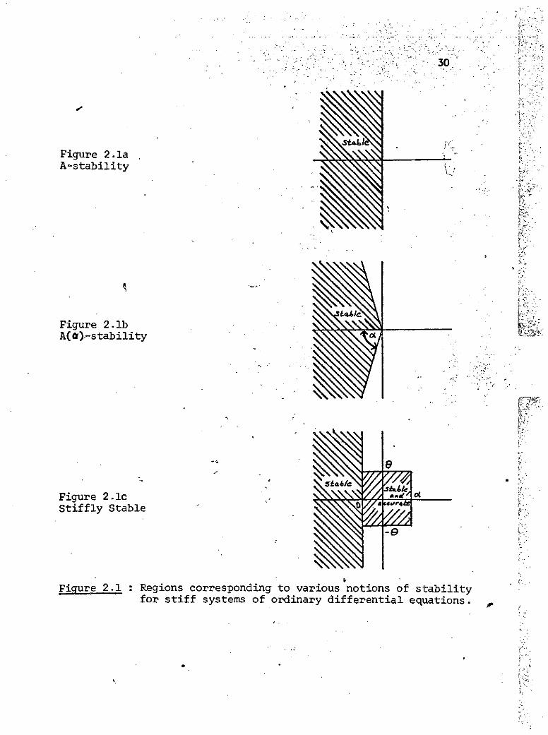
are in a wedge shaped sector in the LHP (see figure 2.1b).

We should note that A(H/2)-stability corresponds precisely to

Dahlquist's A-stability.

Widlund was able to show that for a E [0,H/2) there are

28

A(a)-stable linear multistep methods of orders 3 and 4 (of

derees 3 and 4 respectively). The methods are useful for

many problems, .but if a is close to 1/2 some of the parameters

in the linear multistep methods become very large, thereby

making the methods unsuitable for practical uses in such cases.

There is also the usual difficulty in changing step sizes

because the degrees of the methods are greater than 1.

A second alternative to A-stability was proposed by C.W.

Gear [8], who developed the notion of "stiffly stable" schemes.

Such a scheme would be stable and accurate for eigenvalues in

a rectangular region of the hX-plane which includes the origin

and stable in all parts of the LHP to the left of the rectangle.

(See figure 2.1c.) Gear's criterion has enabled him to produce

up to sixth order linear multistep methods. He also developed

automatic procedures for selecting the step size and order of

the scheme during the calculation. However, the dimensions of

the region of stability that were given by Gear are D -6.1,

8 40.5 and o.zD.1 (see figure 2.1c), which prohibits us from

having eigenvalues lying in the important regions in the LHP

above and below the rectangle.

If there is a single eigenvalue, X, in the unstable region

of the LHP, then one can either increase or decrease h so that

hk falls within the region of stability. However, if there are

several eigenvalues along a ray in the LHP that passes through

the unstable region, it may be very difficult to adjust h so

-29

that all the eigenvalues along the ray fall into the region of

stAbility without making h unduly large or small [27].

Also, because the stiffly stable scheme is variable order

and variable step size, it is exceedingly difficult to get

bounds on the error terms. In addition, there are the usual

difficulties that are associated with any linear multistep method

of degree (number of previous function values needed) greater

than one. Namely, starting values must be computed for the

integration scheme by a special procedure and changing the step

size can be difficult.

C, W. Gear [27] has pointed out that the coefficients used

in the stiffly stable scheme, particularly the sixth order

scheme are not optimal. However, an attempt is being made (in

the United Kingdom) to calculate better coefficients. F. H.

Branin [26] has found that Gear's scheme works quite well on

the whole. During the almost-discontinuous segments of the

solution, the automatic order selection procedure usually

selects the second and third order schemes, and during the

smooth segments, a third through fifth order scheme is usually

selected.

It should be noted that the trapezoidal rule with global

extrapolation can also produce truncation errors of the sixth

or higher orders. It has been found that the trapezoidal rule

with global extrapolation is the most accurate of the integration.

schemes for stiff systems that has been discussed but it is

also one of the most time consuming [141].

-J-

30

Figure 2.laA-stability

Figure 2. b

A(@)-stability

-"

Figure 2. icStiffly Stable "

Figure 2.1 : Regions corresponding to various notions of stabilityfor stiff systems of ordinary differential equations.

31

III. Generalized Trapezoidal Rule

1. Description of the Integration Scheme

The new numerical integration scheme for stiff systems

or ordinary differential equations, that is presented in this

chapter, is a modification of the trapezoidal rule. The

scheme will be called the generalized trapezoidal rule. The

two major aspects of the integration scheme, that differ from

the trapezoidal rule, are:

(1) the use of different numerical integration techniques

for the smooth and the almost-discontinuous segments of the

solution;

and (2) the transformation of the original system of equations,

during the almost-discontinuous segments of the solution, to

a new system of differential equations that is less stiff,

and, consequently, "easier" to integrate.

The transformation employed involves an exponential time

shift, related to the Jacobian of the original system of

equations. The resulting transformed system of equations will

have eigenvalues closer to the origin, and have a lesser

spread between the largest and the smallest eigenvalue than

the original system.

The objectives of the new method are:

(1) to allow the use of larger time steps during the

32

integration of the almost-discontinuous segments of the

solution and still maintain the same or improved accuracy as

compared to the trapezoidal rule,

and (2) to "lessen" the oscillatory problem that is inherent

with the trapezoidal rule (see section 11.5).

Generally speaking, the approach of the proposed

integration scheme is to use the trapezoidal rule with

Newton-Raphson iterations to solve the implicit equations for

calculating the smooth segments of the solution. During the

almost-discontinuous segments, the equations are transformed

to a "smoother" set of equations by means of the transformation

suggested by Lawson [13]. The transformed set of equations

is integrated by means of the trapezoidal rule and both Newton-

Raphson and modified Newton-Raphson iterations are employed

to solve the implicit equations.

The approach described herein differs from Lawson's

generalized Runge-Kutta methods [13] is several respects.

The transformation is applied to an A-stable integration

scheme and is only applied during the almost-discontinuous

segments in conjunction with a linear time shift, in order to

reduce the norms of the matrices involved in the exponential

function; and Newton-Raphson and modified Newton-Raphson

iterations are used to solve the implicit equations in order

to reduce the amount of work per iteration.

A detailed description of the proposed scheme for the

smooth segments is found in section III.la and for the

33

almost-discontinuous segments in section III.lb. Step size

oontrol and techniques for differentiating between the smooth

and almost-discontinuous segments will be discussed in section

III.4.

The integration scheme for the smooth segments is a

relatively standard version of the trapezoidal rule; whereas,

the integration scheme for the almost-discontinuous segments

is a new approach.

la. Calculation of the Smooth Segments

Consider the stiff system of differential equations:

(3.1) * = f(t,x), x(O) = x0.

If one applies the trapezoidal rule:

(3.2a) = x + [ + X n + e(t ,h),

where

(3.2b) e(tnh) = 1 2(8-1)x(3)(t n+ h )d O

is the error term [17], and one Newton-Raphson iteration to

integrate equations (3.1), it can be shown that

(X(0 ) xn - [f(t ,x ) + f(t x(0)(33) x(1) X(0) n+l n 2 n n n+l' n+l(3.3) x xn+l n+l h - (0)

2axj n+1' n+l

where x( 0 ) is an initial approximation to x and x() isn+1 n+l n+

the first corrected approximation to Xn+1 . Usually, the

initial approximation to Xn+ 1 is

(3.4) x() Xn+l n

34

For additional corrected approximations to xn+l, the

Wuperscripts in equation (3.3) are simply increased by one for

each succeeding iteration, and equation (3.3) is repeatedly

iterated until two sucessive approximations to Xn+l differ by

less than some prescribed small amount. When the difference

is small enough, it is said that the sequence of approximations,

fXn('l, has converged to Xn+l .

Equation (3.3) can be rewritten as

(1) (0) hI8f (0) -1 (0)(3.5a) x(1) x - [I - (t0) )]1 vn+l n+l 2 ax/ n+l n+l n+1where

(0) = (0n)+ (0)(3.5b) n (x - x) - 1 f(t ,xn) + f(tn+,n+l

From equations (3.5), it can be seen that the work

necessary for the first Newton-Raphson iteration consists of:

2 function evaluations1 Jacobian evaluation1 matrix inversion1 matrix vector product.

In order to calculate the amount of work necessary to

do the second and later iterations, one must decide whether

Newton-Raphson (NR) or modified Newton-Raphson (MNR) iter-

ations will be used. For the first iteration, equations (3.5),

both types of iterations are identical. For the second and

later iterations, both iterative schemes use equation (3.5),

with superscripts suitably modified. However, in the case

of MNR iterations, the Jacobian matrix is only evaluated

during the first iteration and never reevaluated for succeeding

iterations - that is, the same Jacobian is used for each

35

iteration.

, Hence, in the case of MNR iterations, the second and

later iterations require:

1 function evaluation1 matrix vector product.

In the case of NR-iterations, the Jacobian matrix is

reevaluated for each iteration. Thus, the second and later

iterations require:

1 function evaluation1 Jacobian evaluation1 matrix inversion1 matrix vector product.

W. Liniger [16] pointed out that if the initial approx-

imation, x to xn+1 differed from xn+1 by (h ), gl, then

the first two MNR iterations will differ from Xn+1 by 6(h2g+1

and ((h3g+2) respectively; whereas, the first two NR iterations

will differ from Xn+1 by 0(h2g+l) and ((h4g+3 ) respectively.

If, as suggested, one used equation (3.4) for the initial

approximation to xn+l, then x(0) differs from xn+1 by (h)n+l n+l

--i.e. g =- .---This is true because the trapezoidal rule is

a consistant integration scheme (i.e. its error term is of

order 1 or greater).

One should note that the matrix inverse called for in

equation (3.5a) does not have to be performed. Equation (3.5a)

can be changed so as to allow one to solve a linear system of

equations instead. (It requires fewer operations to solve a

linear system than to invert a matrix.)

36

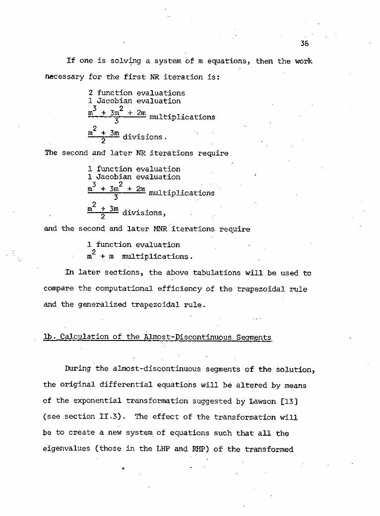
If one is solving a system of m equations, then the work

necessary for the first NR iteration is:

2 function evaluations1 Jacobian evaluation

m + 3m + 2m3 multiplications

2m- + 3mm + 3m divisions.2

The second and later NR iterations require

1 function evaluation1 Jacobian evaluation

3 2m + 3m + 2m3 multiplications

2m + 3m2 divisions,

and the second and later MNR iterations require

1 function evaluation

m2 + m multiplications.

In later sections, the above tabulations will be used to

compare the computational efficiency of the trapezoidal rule

and the generalized trapezoidal rule.

lb. Calculation of the Almost-Discontinuous Segments

During the almost-discontinuous segments of the solution,

the original differential equations will be altered by means

of the exponential transformation suggested by Lawson [13]

(see section II.3). The effect of the transformation will

be to create a new system of equations such that all the

eigenvalues (those in the LHP and RHP) of the transformed

37

system are closer to the origin than the eigenvalues of the

original system. In addition to Lawson's transformation,

time shifts will be performed in order to prevent the norms

of the matrices, that appear in the exponential transformation,

from becoming too large.

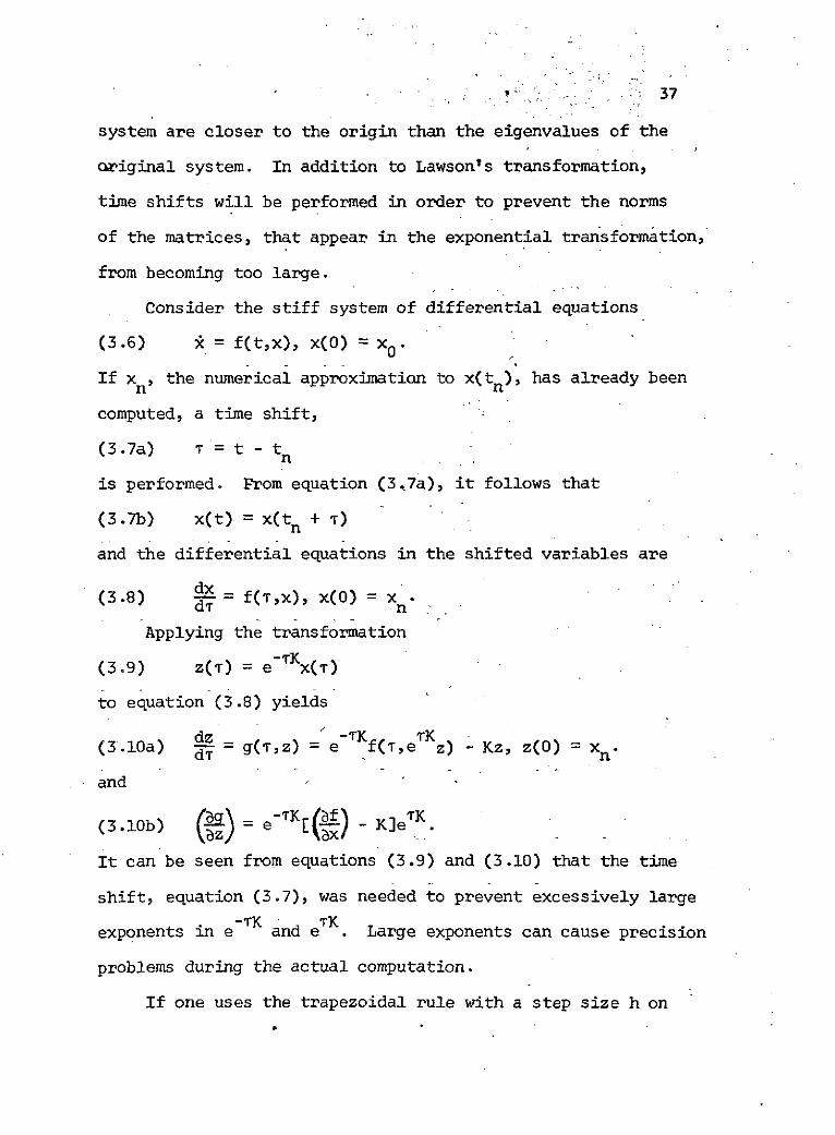
Consider the stiff system of differential equations

(3.6) ) = f(t,x), x(0) = x0 .

If xn, the numerical approximation to x(tn), has already been

computed, a time shift,

(3.7a) 7 = t - tn

is performed. Prom equation (3.7a), it follows that

(3.7b) x(t) = x(tn + 7)

and the differential equations in the shifted variables are

(3.8) dx = f(T,X), X(0) = xdT n

Applying the transformation

(3.9) z(T) = e-TK x(T)

to equation (3.8) yields

-3K

(3.10a) d- g(T,z) = e f(T,e z) Kz, z(0) = x

and

(3.10b) ) = e-K[ - K]eK.

It can be seen from equations (3.9) and (3.10) that the time

shift, equation (3.7), was needed to prevent excessively large-TK n TK

exponents in e and e . Large exponents can cause precision

problems during the actual computation.

If one uses the trapezoidal rule with a step size h on

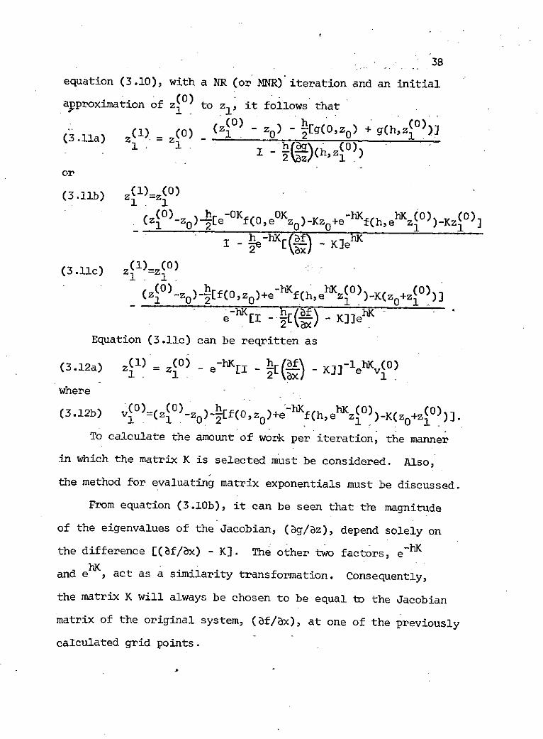
38

equation (3.10), with a NR (or MNR) iteration and an initial

approximation of z(0) to zl, it follows that

(3.11a) z)= z(0) (z0 z) - g(0,z 0 ) + g(h,z( 0 )lI -1.~ 2 (hzl )

or

(3.11b) z(l)-z (0)1 1

(0) h -OK OK -hK hK (0) (0)(z 1 -z 0 ) 21e f(0,e z 0 )-Kz 0 +e f(h,e z 1 )-Kzl ]

h -hK (af KI - e [L- - KIe h K

(3.11c) z(1)=z(0 )

1 1(0) h -hK hK (0) (0)(z( -z 0 )-h[f(0,z 0 )+e f(h,e hl )-K(z 0 +z( )

e-hK _ h /f Ke [I 1 - K]]e

Equation (3.11c) can be reqritten as(3.12a) z(1) (0) e-hK i h lf\ KX]-lehK (0)

where

(3.12b) (0)=(z(0) -z 0 ) f(0,z 0 )+e - h Kf(h,ehKz ( 0 ) ) -K(z+z 0)

To calculate the amount of work per iteration, the manner

in which the matrix K is selected must be considered. Also,

the method for evaluating matrix exponentials must be discussed.

From equation (3.10b), it can be seen that tle magnitude

of the eigenvalues of the Jacobian, (6g/bz), depend solely on

the difference [(bf/bx) - K]. The other two factors, e - h K

and e hK , act as a similarity transformation. Consequently,

the matrix K will always be chosen to be equal to the Jacobian

matrix of the original system, (bf/6x), at one of the previously

calculated grid points.

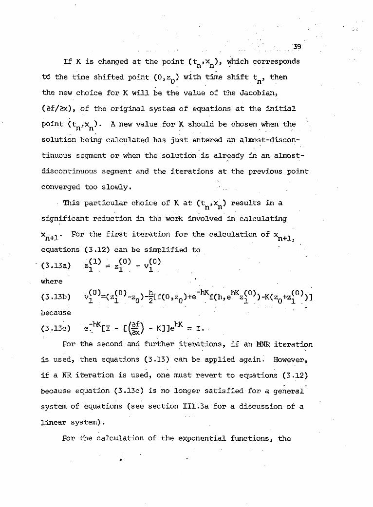
'39

If K is changed at the point (t ,x ), which correspondsn n

tc the time shifted point (O,z0) with time shift tn, then

the new choice for K will be the value of the Jacobian,

(af/ax), of the original system of equations at the initial

point (tn,x ). A new value for K should be chosen when the

solution being calculated has just entered an almost-discon-

tinuous segment or when the solution is already in an almost-

discontinuous segment and the iterations at the previous point

converged too slowly.

This particular choice of K at (tn,Xn) results in a

significant reduction in the work involved in calculating

Xn+l o For the first iteration for the calculation of Xn+1,

equations (3.12) can be simplified to((l) (0) (0)

(3.13a) z1 = 1 1

where

1 1 ()z() z )--[f(0,zo)+e-hKf(h,e z 1 ))-K(z0+z()

because

(3.13c) e-hK[I - ) - K]]e = I.

For the second and further iterations, if an MNR iteration

is used, then equations (3.13) can be applied again. However,

if a NR iteration is used, one must revert to equations (3.12)

because equation (3.13c) is no longer satisfied for a general

system of equations (see section III.3a for a discussion of a

linear system).

For the calculation of the exponential functions, the

40

diagonal Pade approximations will be used because they are

Arstable and make optimal use of the powers of the matrix, hK,

that will be computed. In particular, either the Ell or E22

approximations,

(3.14) E11(hK) = [I - K1 + 1 + j )

(3.15) E2 2 (hK) = [I - hK + 1 K) 2 -1I +K + 2

+a( JhK 115)

will be used because their error terms are of the same or

slightly better order than the generalized trapezoidal rule.

It is important to note that if global extrapolation is to be

used, a higher order Pade approximation may be necessary

(see section 11.7).

In order to get increased accuracy in the Pade approx-

imations, the argument reduction scheme,

(2-ShK) 2 hK(3.16) e 2 ] 2 e

is used. The bracketed expression is calculated using E11 or

E22 and then squared s times. Equation (3.16) effectively

decreases the norm of the argument of the Pade approximation

and thereby increases the accuracy of the approximation. In

practice, s = 4 or 5 is usually sufficient [19]. In section

III.3b, there is a more detailed discussion of the error in

the Pade approximation.

To calculate the amount of work per iteration, two pairs

of cases must be considered: using a new value for K, and using

an old value for K. For each

41possibility for K, either an NR or an MNR iteration can be used

for the second and further iterations. In addition to the work

per iteration, there is one extra matrix-vector product needed

to obtain xn+1 from z .

When selecting a new value for K, the amount of work for

the first NR (or MNR) iteration, using equations (3.13), is

2 function evaluations1 Jacobian evaluation (for K)2 Pade approximations3 matrix-vector products1 matrix-scalar product.

For the second and later MNR iterations, equations (3.13) can

still be used. The work per iteration is

1 function evaluation3 matrix-vector products1 matrix-scalar product.

However, for the second and later NR iterations, one requires :

1 function evaluation1 Jacobian evaluation1 matrix inversion6 matrix-vector products1 matrix-scalar product.

Clearly, it is preferable to use MNR iterations since a NR iter-

ation requires much more work per iteration than a MNR iteration.

When using an old value of K, all iterations must make use

of equations (3.12). The first iteration requires

2 function evaluations1 Jacobian evaluation1 matrix inverse6 matrix-vector products1 matrix-scalar product.

For the second and later iterations, an MNR iteration requires

42

1 function evaluation6 matrix-vector products,

and a NR iteration requires

1 function evaluation1 Jacobian evaluation1 matrix inverse6 matrix-vector products1 scalar-matrix product.

Again one should note that the matrix inverse called for

in equation (3.12a) and indicated above does not have to be

performed. Equation (3.12a) can be changed so as to allow one

to solve a linear system of equations instead.

When one is solving a system of m equations, and has

selected a new value for K, the amount of work for the first

iteration is

2 function evaluations1 Jacobian evaluation2 Pade approximations

4m2 + m multiplications.

The second and later MNR iterations require

1 function evaluation

4m2 + m multiplications,

and the second and later NR iterations require

1 function evaluation1 Jacobian evaluation

m + 21m2 + 2m3 multiplications

m + 3m divisions.2

However, when an old value of K is being used, then the first

NR iteration requires

43

2 function evaluations1 Jacobian evaluation3 2

m + 21m + 2m multiplications

m- + 3m2 3m divisions.2

The second and later MNR iterations need

1 function evaluation

6 m2 + m multiplications,

and the second and later NR iterations need

1 function evaluation1 Jacobian evaluation3 2m + 21m2 + 2m3 multiplicationsm + 3m3

divisions.2

In the later sections of this chapter, it will be shown

that the generalized trapezoidal rule is computationally more

efficient than the trapezoidal rule for computing almost-

discontinuous segments. The theoretical error comparisons and

illustrative computer results presented later indicate that the

generalized trapezoidal rule requires more work per iteration

but the overall amount of work needed to compute the almost-

discontinuous segment is less than that required by the trap-

ezoidal rule.

2. Rationale of the Integration Scheme

When an A-stable integration scheme is being chosen to

solve a stiff system of ordinary differential equations, a

44

decision must be made as to how much detail one wishes to see

in.,the various segments of the solution. This decision is

particularly crucial for the calculation of the almost-discon-

tinuous segments of the solution.

If one wishes to obtain extremely fine details of the

structure of the solution during an almost-discontinuous seg-

ment, then extremely small step sizes of the order of the small-

est time constant must be used. In that case, the present

author and others [5] have suggested that high order explicit

schemes, such as fourth and fifth order Runge-Kutta schemes, be

used for the almost-discontinuous segments of the solution.

The small step size (or perhaps a reasonable fraction of it

such as 1/2 or 1/4) satisfies the stability criterion for explicit

schemes and the explicit schemes are much easier to implement

(there are no implicit equations to solve).

However, during the smooth portions of the solution, an

A-stable scheme will probably be needed because the desired

step sizes will probably be outside the region of stability for

a step length limited scheme. It remains to be proved that

the use of an explicit scheme within it's region of stability

does not cause stability problems.when one switches to an A-stable

scheme to calculate the smooth segments of the solution, although

it is probably true.

The generalized trapezoidal rule proposed herein is not

meant for obtaining very fine detailed solutions during the

45

almost-discontinuous sections. The basic aim of the scheme is

to transform the original equations to a new system of equations

such that the eigenvalues of the transformed system are smaller

in magnitude than the eigenvalues of the original system, and

the ratio of the real parts of the largest to the smallest

eigenvalue of the transformed system is smaller than the same

ratio for the original system. A consequence of shifting the

eigenvalues is that for the same accuracy, one can integrate the

new system of equations with a larger time step than is possible

for the original system. However, a larger time step means

that one cannot expect to see as much fine detail as for a

smaller time step.

Therefore, the proposed scheme is primarily suggested for

the integration of systems of equations where one wishes to see

a moderate to coarse degree of detail, but with a relatively

high degree of accuracy, for the almost-discontinuous segments,

and is not interested in very fine detail. The proposed scheme

allows one to solve a smoother set of equations at the expense

of having to calculate a difficult transformation and having to

do more work per step than the trapezoidal rule. However, in

the almost-discontinuous segments, the extra work is more than

compensated for by allowing one to use larger time steps when

solving the transformed equations as compared with solving the

original equations.

The other consideration in the proposed scheme is that

46

the smooth and almost-discontinuous segments are calculated

dfferently. The reasoning behind this decision is that simple

A-stable schemes, such as the trapezoidal rule, work

very will when the solution, over the particular region being

integrated, is smooth. A transformation whose objective is to

smooth out the solution in a smooth region cannot help very

muchsince the solution of the original system is already

smooth. Therefore, the extra work necessary for computations

using the generalized trapezoidal rule, as compared with the

trapezoidal rule, probably cannot be favorable compensated for

by an increase in the step size (to be illustrated in section

III.3a).

3. Theoretical Error Calculations

The trapezoidal ruleand the generalized trapezoidal rule

discussed in section III.1 are both second order schemes.

However, it is constructive to compare the errors produced by

each scheme when each is applied to several examples where the

exact error can be calculated. In section III.3a, three examples

are considered and the errors in the numerical solution using

each scheme are calculated and tabulated for various step sizes.

In section III.3b, the errors incurred when one uses the

Pade approximation, Ell and E22 , are discussed and tabulated.

The reduction in the error as a result of using the argument

scheme (3.16) is also considered. Errors for other Pade

47

approximations can be found in [193.

3a. Theoretical Errors for Various Ordinary DifferentialEquations-*

In each example, it will be assumed that all exponential

functions can be calculated exactly. The errors incurred

in calculating the exponentials will be discussed in the

next section. Also, all calculations will be based on

a fixed step size.

Example 1:

The first example that will be considered is the stiff

linear time invariant system

(3.17) * = Ax, x(O) = x0

When the exponential transformation,

-tC(3.18) z = e x,

is applied to (3.17), it follows that

(3.19) dz = e tCAe tCz - Cz z(0) = x

If C = A, then equation (3.19) reduces to

(3.20) z' = 0, z(O) = x 0

which can be solved exactly --i.e. no error is incurred in.

the numerical solution.

However, if C ) A, but C ; A and C and A commute, then

* The second and third examples in this section were

suggested by [5].

48

it follows that

dz(3. 21) = (A-C)z, z(0) = x0

If we have that

p(A-C) << p(A)

where p(A) is the spectral radius of A, then the trapezoidal

rule will give more accurate results for equation (3.21)

than for equation (3.17). Equivalently, for the same accuracy,

one can take larger steps when integrating equation (3.21)

than when integrating equation (3.17). Also, since the

trapezoidal rule applied to a linear system is equivalent

to using the Ell Pade approximation (without using the argument

reduction scheme), the errors in the computation can be found

on tables (3.3) and (3.4) in section III.3b.

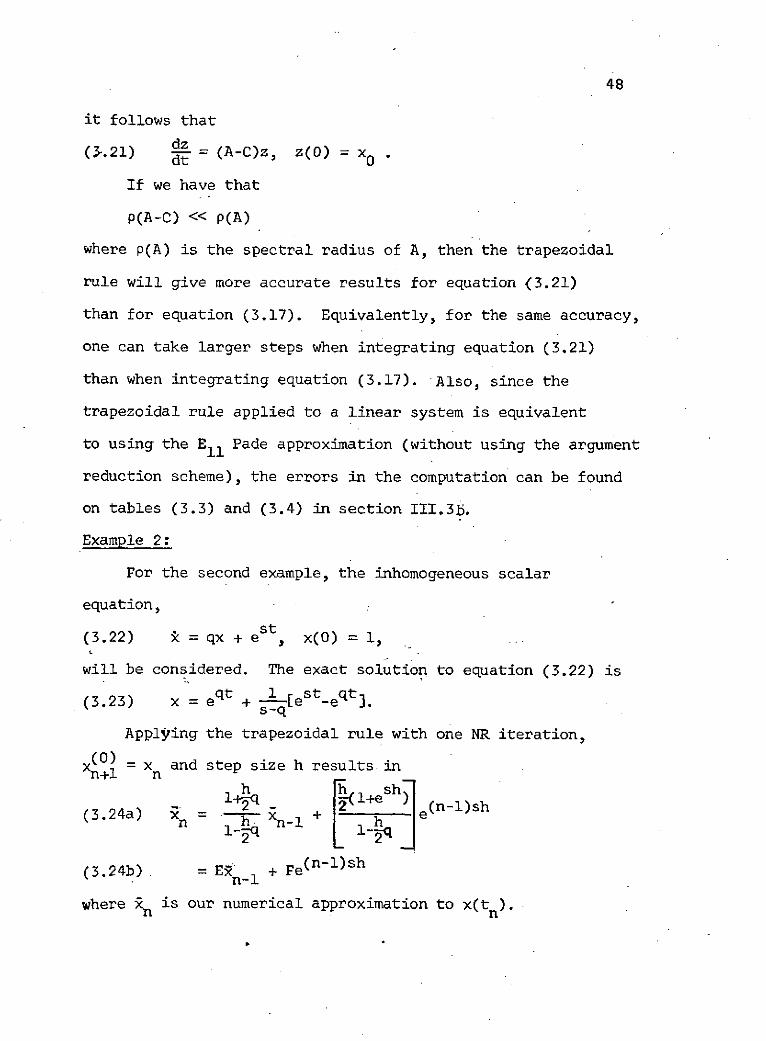
Example 2:

For the second example, the inhomogeneous scalar

equation,

st(3.22) = qx + e , x(O) = l,

will be considered. The exact solution to equation (3.22) is

(3.23) x = eq t + st-eqt.

Applying the trapezoidal rule with one NR iteration,

xn(0) = x and step size h results in1n+l n

(3.24a) Xn = -h- xn_1 + e_-n h

(3.24b) :E"n I Fe

where n is our numerical approximation to x(tn).n n

49,

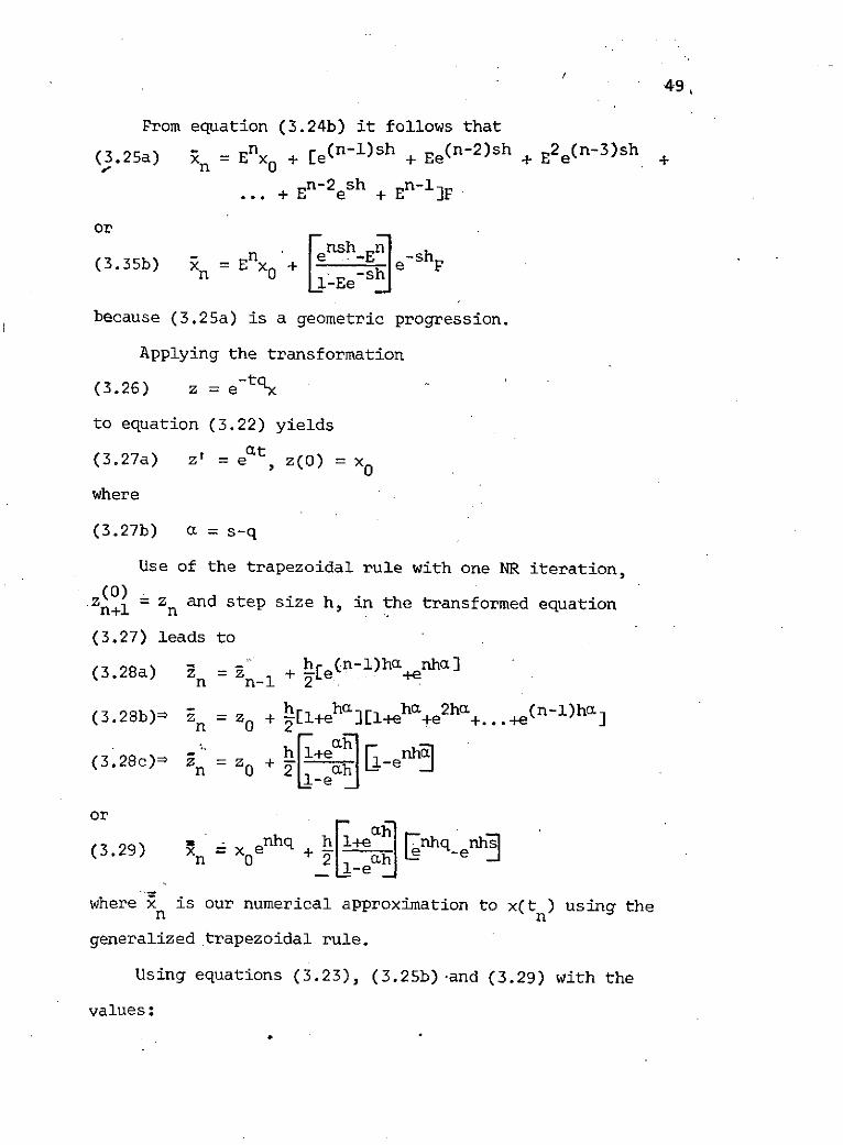
From equation (3.24b) it follows that

(3.25a) n = Ex+ [e(n-l)sh + Ee(n-2 )sh + E2 e(n-3 )sh +

En-2 sh En-1IF.. +E e +E ]F

orn sh Sh

(3.35b) n = nx + se e-h

because (3.25a) is a geometric progression.

Applying the transformation

(3.26) z = e-tq

to equation (3.22) yields

(3.27a) z = eat z() = x0

where

(3.27b) a = s-q

Use of the trapezoidal rule with one NR iteration,

(0)Zn+l = Zn and step size h, in the transformed equation

(3.27) leads to

h[ (n-1)h nhcL](3.28a) n = n 1 + hre(n-)ha na]

h ha ha 2ha (n-1)ha(3.28b)= zn = z0 + [l+e [1+e +e +...+e]

"- h 1+eLh e(3.28c)= * n = z0 + 2[ah] en

or

(3.29) n x0 e +nhq h +eh -enh

where xn is our numerical approximation to x(t ) using the

generalized trapezoidal rule.

Using equations (3.23), (3.25b)-and (3.29) with the

values:

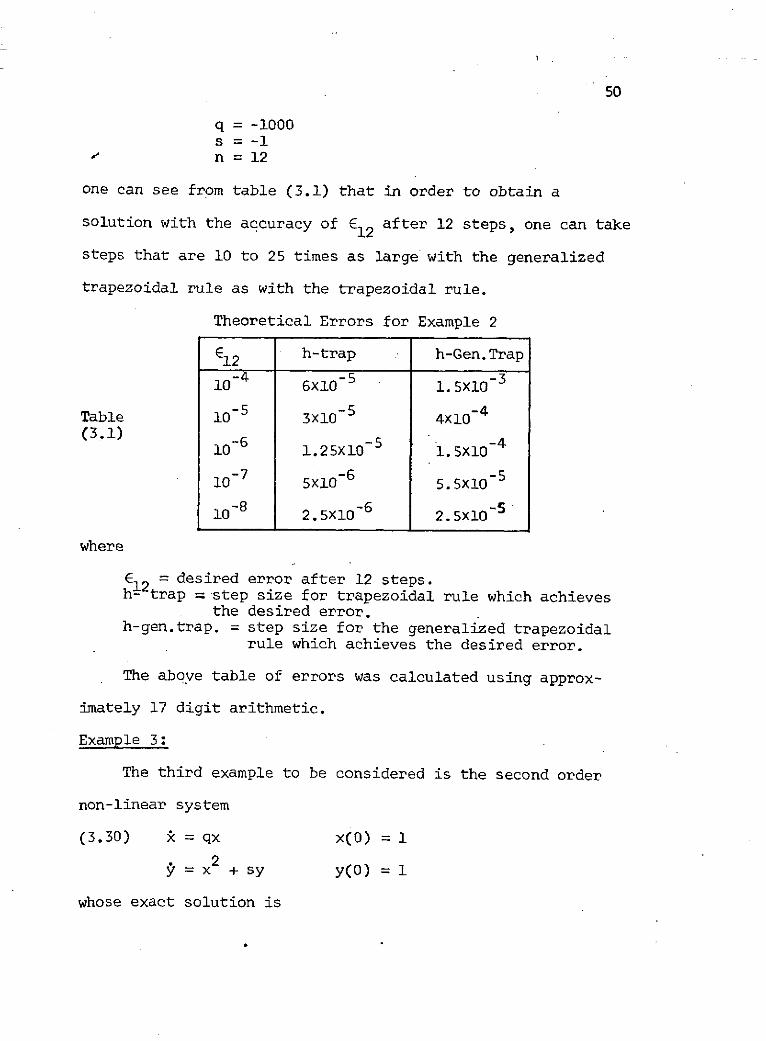
50

q = -1000s = -1n =12

one can see from table (3.1) that in order to obtain a

solution with the accuracy of E12 after 12 steps, one can take

steps that are 10 to 25 times as large with the generalized

trapezoidal rule as with the trapezoidal rule.

Theoretical Errors for Example 2

E12 h-trap h-Gen.Trap

-4310-4 6X10-5 1.5xl10 -3

Table 10-5 3x10-5 4x10-4(3.) 10-6 -5 -410 1.25X10 1.5xl0

10-7 5x10 -6 5.5X10-5

10 2.5xl0-6 2.5x10 -5

where

E12 desired error after 12 steps.h- trap =-step size for trapezoidal rule which achieves

the desired error.h-gen.trap. = step size for the generalized trapezoidal

rule which achieves the desired error.

The above table of errors was calculated using approx-

imately 17 digit arithmetic.

Example 3:

The third example to be considered is the second order

non-linear system

(3.30) k = qx x(0) = 1

2y = x + sy y(O) = 1

whose exact solution is

51

(3.31) x = x0et2

st 0 2qt sty = y0 e + 2q-se -e ]

By applying the transformation

(3.32) (u) = e-Jt()

where J is the Jacobian of equations (3.30), it follows that

d = 0 ,u(0) = x0(3.33)

S= e(2q-S)tu2 - 2x0e( -S)t u ,v(0) = YO

If one applies the trapezoidal rule to equations .(3.30),

one has that

F h1-

Xn h x0

(3.34a) n K nE 2nyn = E + K 1 2

1. 2

where

" i--s h F1+h -77 h 2 (3.34b) E1 E2 = -- K = h h +

1- -)(-) l-

The use of the generalized trapezoidal rule to equations

(3.30) yields

x qnhxn = 0e

22x qnh snh

Sq-s

snhxh 2 +eh 1-enh+ e (2)x 0 Ll+e h

1-e+ eShx02 [l+e h ]

52

where

(.3.35b) a = 2q - s

S=q -s

Using equations (3.31), (3.34), and (3.35) with the

values:

q = -1000s = -1n =12

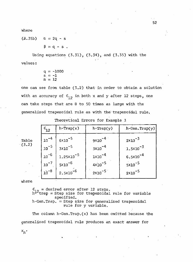
one can see from table (3.2) that in order to obtain a solution

with an accuracy of 612 in both x and y after 12 steps, one

can take steps that are 8 to 50 times as large with the

generalized trapezoidal rule as with the trapezoidal rule.

Theoretical Errors for Example 3

E12 h-Trap(x) h-Trap(y) .h-Gen.Trap(y)

-4 -5 -4 3Table 10 6x10-5 910-4 2x10 3

(3.2) -5 -51 3X0 3X10 1.5XI0

10 - 6 1.25X10-5 IXlO-4 6.5X10- 4

10 - 7 5x10 - 6 4xi0- 5 5X10 - 5

-8 -6 -5 -510 2.5x10 2X10 2X10

where

E = desired error after 12 steps.h- trap = Step size for trapezoidal rule for variable

specified.h-Gen.Trap. = Step size for generalized trapezoidal

rule for y variable.

The column h-Gen.Trap.(x) has been omitted because the

generalized trapezoidal rule produces an exact answer for

Xn

53

When looking at the results of the calculation for the

third set of equations (3.30), one must remember that in

the solution, x is rapidly changing, but y is slowly changing.

From equations (3.31), one can see that y goes as e-st with

a slight perturbation due to the second term. For s = -1

and q = -1000, the perturbation is less than 1/2000 --i.e.

it shows up in the third or fourth decimal places at most.

Thus, when using the trapezoidal-rule to integrate equation

(3.30), it is the x equation that determines the step size

at the beginning of the numerical computation.

If one compares the step sizes for y in table (3.2),

one can see that there is not that much difference between

them. But, the solution to the y equations is smooth and we

should not expect a smoothing process to signigicantly

decrease the required step size. For this reason the

transformation should be applied only during the almost-

discontinuous segments and not during the smooth segments.

3b. Accuracy of the Pade Approximations [19]

The Pade approximations are useful for computing e t

where M is an n x n matrix, when the stability of the

approximation is an important criterion. For the Pade approx-

imations, one sets

(3.36) etM Ep,q(tM) = N (tM)D (tM)p,q

54

where N and D are polynomials with real coefficients andpq pq

of orders q and p respectively. The coefficients of N and

D are chosen so that E agrees with the Taylor series expansion

of etM through and including terms of order (p+q). This

requirement leads to the equations [25]

N pq(tM) = (p+-k)q (tM)kp,q k=(P+q) kl(q-k).

(3.37)p (k+o-k) , k

D (tM) = E (+-k tM) k

p,q k=O (p+q)k!(p-k)t

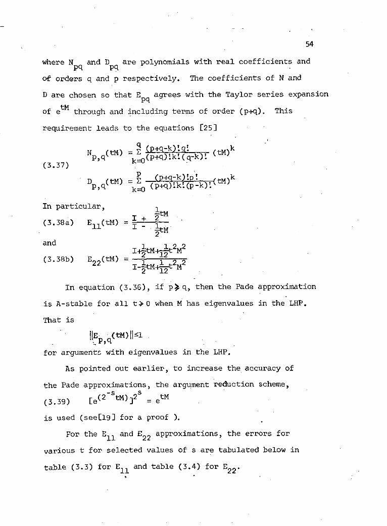
In particular, 1

(3.38a) E11(tM) =I 1I - 1-tM

and 1 2 2

(3.38b) E22 (tM)22 = 1 1 2 2

In equation (3.36), if p)q, then the Pade approximation

is A-stable for all t) 0 when M has eigenvalues in the LHP.

That is

IJEp (tM) I<l.pq

for arguments with eigenvalues in the LHP.

As pointed out earlier, to increase the accuracy of

the Pade approximations, the argument reduction scheme,

(3.39) [e(2StM) 12 = e

is used (see[19] for a proof ).

For the E11 and E22 approximations, the errors for

various t for selected values of s are tabulated below in

table (3.3) for Ell and table (3.4) for E22.

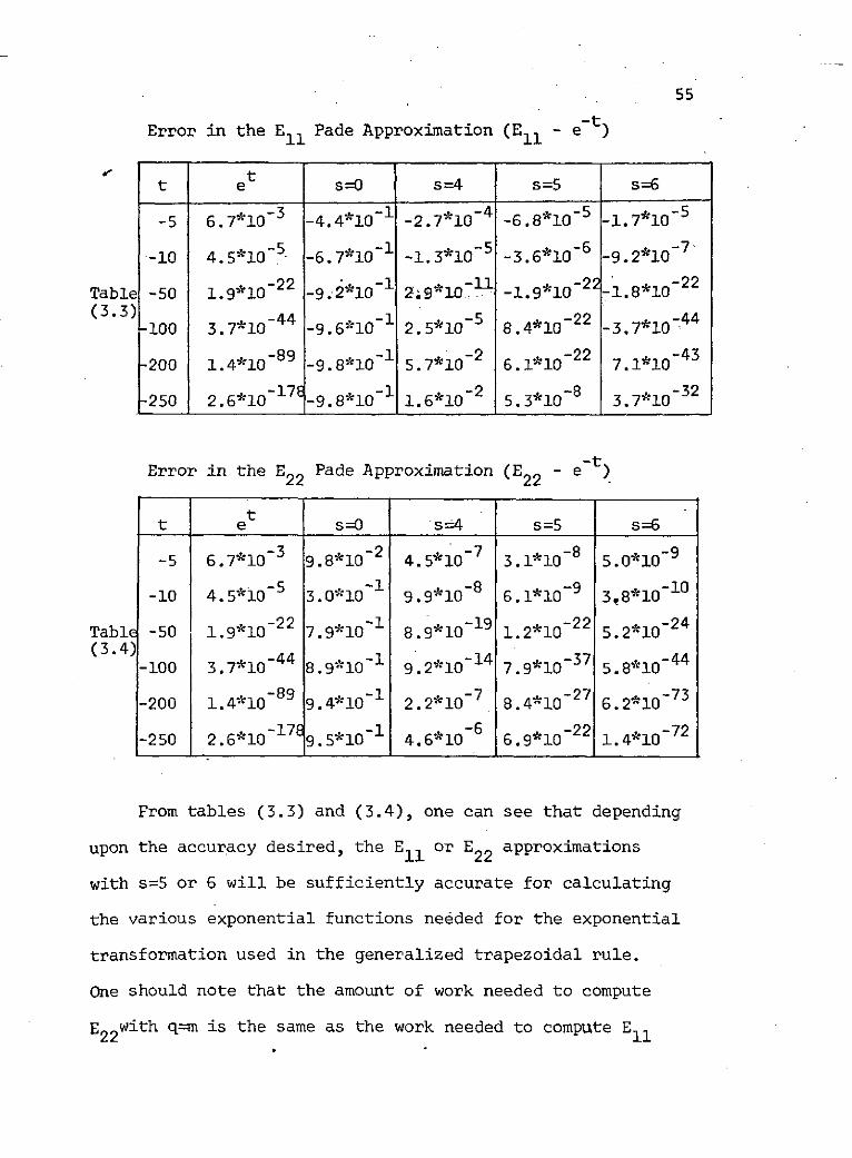
55

-tError in the E11 Pade Approximation (E11 - e t)

tt e s=0 s=4 s=5 s=6

-5 6.7*10-3 -4.4*10-1 -2.7*10 - 4 -6.8*10 - 5 -1.7*10 - 5

-10 4.5*10-5 -6.7*10-1 -1.3*10-5 -3.6*10-6 -9.2*10-7 -

4 22 -1 11-622Table -50 1.9*10-22 -9.2*i10 - 29*0 - - -1.910 -2 .8*10 - 22(3.3) -44 J 1 2.5.105 22 -44

-100 3.7*10- -9.610 2.510 8.4*10-22 -3.7*1044

200 1.4*10-89 -9.8*10- 1 5 .7*10 -2 6.1*10-22 7.1*10-43

250 2.6*10-17 9.8*10-1 1.6*10-2 5.3*10-8 3.7*10 -32

Error in the E22 Pade Approximation (E22 - e-t )

t e s=0 s=4 s=5 s=6

-5 6.7*10 - 3 9.8*10- 2 4.5*10- 7 3.1*10- 8 5.0*10- 9

-10 4.5*10 -5 3.0*10-1 9.9*10-8 6.1*10- 9 3,8*1010

TablE -50 1.9*10-22 7.9"10- 1 8.9*10- 19 1.2*10- 2 2 5.2"10- 2 4

(3.4) -100 3.7*10- 44 8.9*10- 1 9.2*1014 7.9*1037 5.8*10

-200 1.4*10 - 89 9.4*10- 1 2.2*10- 7 8.4*10- 27 6.2*10 - 73

-250 2.6*10-17 9 . 5* 1 0 - 1 4.6*10-6 6.9*10- 22 1.4*10 - 72

From tables (3.3) and (3.4), one can see that.depending

upon the accuracy desired, the E 1 or E22 approximations

with s=5 or 6 will be sufficiently accurate for calculating

the various exponential functions needed for the exponential

transformation used in the generalized trapezoidal rule.

One should note that the amount of work needed to compute

E22with q=m is the same as the work needed to compute E11

56with s = m+l. However, the E22 approximation with s = m is

more accurate than the E11 approximation with q = m+l.

Therefore, the E22 approximations will be used for computations.

4. Step Size Control and Detection of Almost-DiscontinuousSegments

For a particular problem, the user always specifies

the maximum step size, h . For example, h is at mostmax max

the sample period for the solution or the points at which

the user wishes to see the value of the solution over the

range of integration. To begin calculating the solution, it

will be assumed that one will calculate an almost-discontinuous

segment (unless told otherwise) and begin with a step size

h = hmax/16. The reason for the 1/16 is that the user may

have specified a large hmax, and, if h is too large, too

many iterations may have to be done before the approximations

to the next point converge.

During the smooth segments, the step size control that

will be used is a standard method based on counting the

number of iterations necessary to solve the implicit

trapezoidal rule equations (3.2). If it takes one or two

iterations for the approximations to Xn+ 1 to converge,

then the step size, h, will be doubled for the calculation

of the next point. However, if the approximations have

not converged after four iterations, then the results of

the iterations will be discarded and the calculation will

57

be repeated with half as large a step size as the one that

failed.

For the almost-discontinuous segments, the amount of

work needed for changing the step size --except for doubling

the step size, which requires two matrix multiplications,

or else two matrix-vector procucts and some bookkeeping--

is considerable because e-hK and ehK must be recomputed.

Therefore, the rule of thumb used for changing step sizes

will be that if the approximation to zl converges in two

or fewer iterations, h will be doubled, but if it takes

more than five iterations then h will be halved and K reselected.

The reselection of K whenever h is halved is done in order to

reduce significantly the work for the first iteration with

the new h --i.e. one uses equations (3.13) instead of (3.12).

The reason for changing h after five iterations, instead of

four as in the smooth segments, is that changing h requires

alot of work.

The detection of whether one is calculating a smooth

segment or an almost-discontinuous segment is at best a difficult

task. If one does not have a priori information about the

nature of the solution or the location of the smooth and

almost-discontinuous segments then there are two available

alternatives. One can calculate finite difference approxima-

tions to the derivative of each variable or one can count the

number of NR (or MNR) iterations needed to obtain the

58

solution to the implicit integrating equations. The latter

approach will be chosen.

The procedure that will be used is as follows:

(1) if one is calculating an almost-discontinuous segment

and the step size for the next step will exceed hmax/A , then

one will say that one is in the smooth region and change to

the integration of a smooth segment of the solution; but

(2) if one is calculating a smooth segment and the step

size for the next step will be less than h max/32, then

one will say that one is in the almost-discontinuous region

and change to the integration of an almost-discontinuous step.

The cross-over point between the two types of segments

is not the same in both directions. This is intentional and

is meant to prevent the numerical technique from oscillating

back and forth between the two phases of the integration

scheme. If rapid oscillations between the two phases were

permitted, then the value of the approach in the almost-

discontinuous segments might be nullified due to the initial

overhead involved.

5. Illustrative Computer Results

In this section, the results of actual numerical comput-

ations using both the generalized trapezoidal rule and the

trapezoidal rule will be presented. The examples chosen are

the same as those analysed in section III.3a (Theoretical

- 59

Error Calculations).

For the linear equations, the exponential functions

needed for the generalized trapezoidal rule were evaluated

by means of the E11 Pade Approximation with s = 5. However,

for the inhomogenous equations and the non-linear equations,

the E22 Pade approximation with s = 5 was used. In each

example, the step size was controlled by means of the method

suggested in section 111.4. All computations were done in

PL1 to approximately 17 decimal places on the IBM 360/91.

Example 1:

For the linear equation

(3.40) ; = qx, x(O) = 1.

the solutions were computed over the interval t = (0,.25)

for q = -10, -100, and -1000. Maximum step sizes of h = .1

and .01 were used.

In the tables below, "error" means the error in the

numerical solution at t = .25. "Oscillates" means that the

numerical solution was oscillating because the step size

was too large, and that the indicated error is a poor measure

.of the solution over the entire interval t = (0,.25). "Iter"

refers to the number of Newton-Raphson iterations needed to-8

obtain the solution. Also, an error of 10 means that the

error occurred in a decimal position beyond the last decimal

digit printed out.

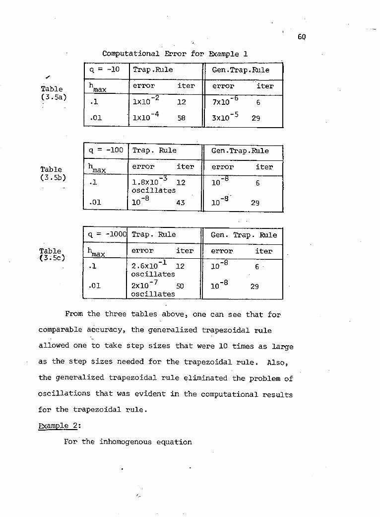
60

Computational Error for Example 1

q= -10 Trap.Rule Gen.Trap.Rule

Table hmax error iter error iter

(3.5a) .1 lxl0-2 12 7x10 6 6

-4 -.01 lxl0 -4 58 3x10-5 29

q = -100 Trap. Rule Gen.Trap.Rule

Table hmax error iter error iter(3.5b) .1 1.8x10 -3 12 10-8 6

oscillates

.01 108 43 10- 29

q = -1000 Trap. Rule Gen. Trap. Rule

Table hmax error iter error iter.(3.5c) max

.1 2.6x10 12 108 6oscillates

.01 2x10-7 50 10-8 29oscillates

From the three tables above, one can see that for

comparable accuracy, the generalized trapezoidal rule

allowed one to take step sizes that were 10 times as large

as the step sizes needed for the trapezoidal rule. Also,

the generalized trapezoidal rule eliminated the problem of

oscillations that was evident in the computational results

for the trapezoidal rule.

Example 2:

For the inhomogenous equation

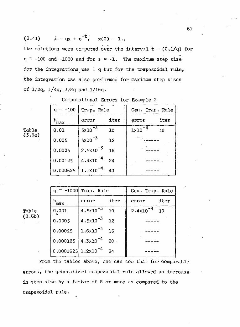
61

-t(3.41) : = qx + e , x(0) = 1.,

the solutions were computed over the interval t = (0,1/q) for

q = -100 and -1000 and for s = -1. The maximum step size

for the integrations was 1 q but for the trapezoidal rule,

the integration was also performed for maximum step sizes

of 1/2q, 1/4q, 1/8q and 1/16q.

Computational Errors for Example 2

q = -100 Trap. Rule Gen. Trap. Rule

h error iter error itermax

Table 0.01 5x10 - 3 10 lxl0-4 10(3.6a) -3

0.005 5xl0 12-3

0.0025 2.5xl0 16 -----

-40.00125 4.3x10- 4 24 -----

0.000625 1.1xl0 -4 40 -----

q = -1000 Trap. Rule Gen. Trap. Rule

h error iter error itermax

Table 0.001 4.5x10- 3 10 2.4xl0 -4 10(3.6b) 1

0.0005 4.5x0 -3 12 -----

-30.00025 1.6x10 - 3 16 -----

0.000125 4.3x10 - 4 20

-0;0000625 1.2X10 -4 24

From the tables above, one can see that for comparable

errors, the generalized trapezoidal rule allowed an increase

in step size by a factor of 8 or more as compared to the

trapezoidal rule.

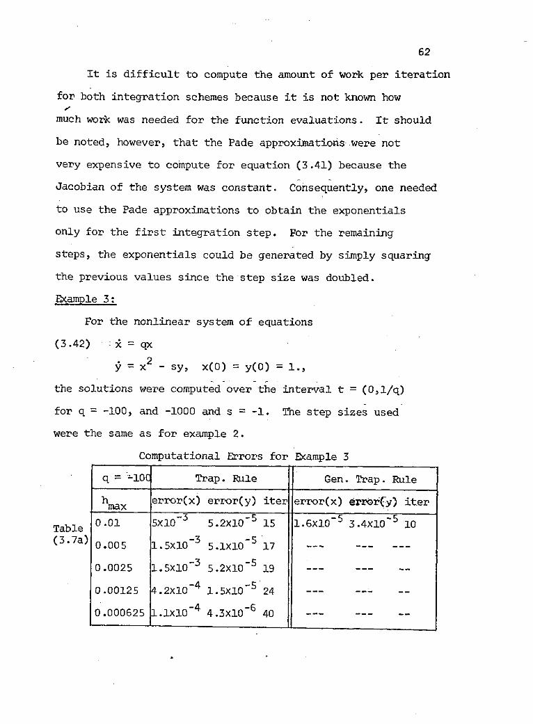
62

It is difficult to compute the amount of work per iteration

for both integration schemes because it is not known how

much work was needed for the function evaluations. It should

be noted, however, that the Pade approximations .were not

very expensive to compute for equation (3.41) because the

Jacobian of the system was constant. Consequently, one needed

to use the Pade approximations to obtain the exponentials

only for the first integration step. For the remaining

steps, the exponentials could be generated by simply squaring

the previous values since the step size was doubled.

Example 3:

For the nonlinear system of equations

(3.42) i = qx

= X2 - sy, x() = y(O) = 1.,

the solutions were computed over the interval t = (0,/q)

for q = -100, and -1000 and s = -1. The step sizes used

were the same as for example 2.

Computational Errors for Example 3

q = -10C Trap. Rule Gen. Trap. Rule

hma x error(x) error(y) iter error(x) error{y) iter

Table 0.01 5X10 - 3 5.2X10-5 15 1.610 - 5 3.4xl0- 5 10

-3 -5(3.7a) 0.005 1.5x10-3 5.lxlO-5 17 --- --- ---

0.0025 1.5X10 3 5.2X10 19 --- --- --

0.00125 4.2x10- 4 1.5X10 - 5 24 -- --- --

0.000625 .1xl0-4 4.3X10 40 --- --

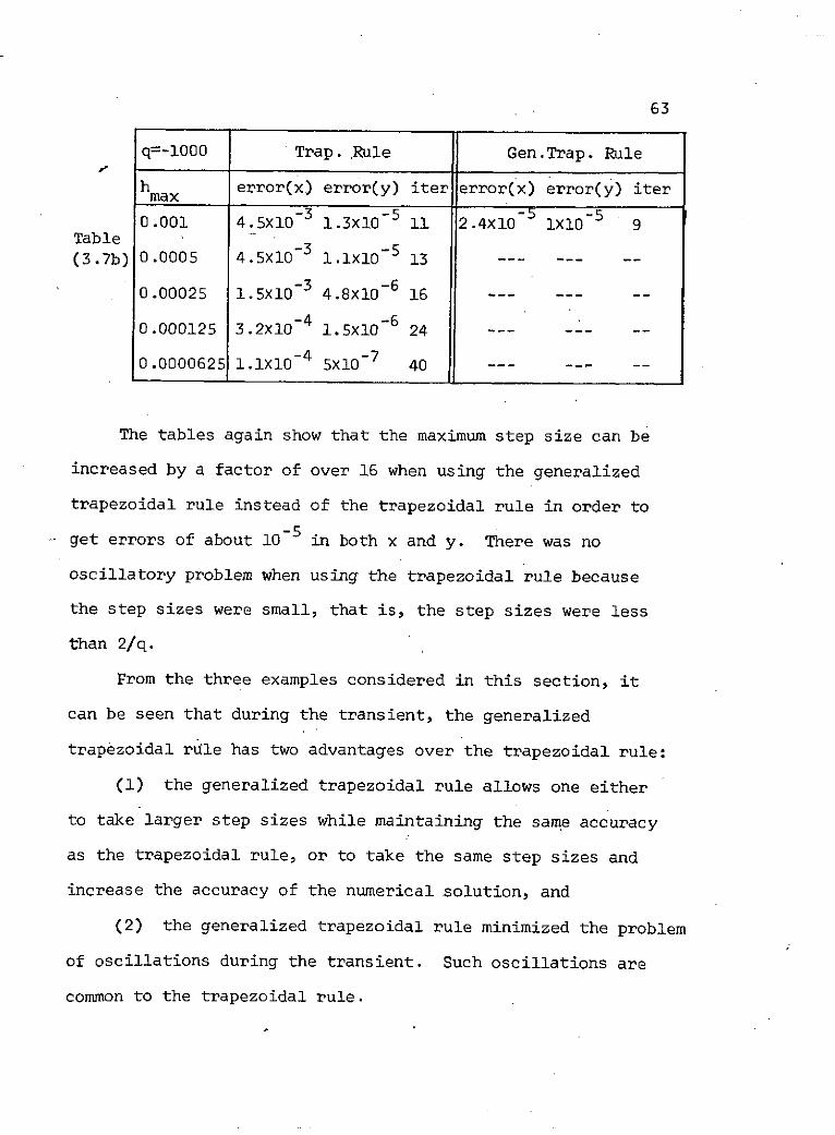
63

q=-1000 Trap. Rule Gen.Trap. Rule

hmax error(x) error(y) iter error(x) error(y) iter

0.001 4.5X10 -3 1.3X10 - 5 11 2.4X10 l0l - 9Table 3(3.7b) 0.0005 4.5x10 1.1xl0- 5 13 --- --- --

0.00025 1.5x10-3 4.8x10- 6 16 --

-4 -60.000125 3.2x10 - 4 1.5X10 - 6 24 --- --- --

0.0000625 1.lxl0- 4 5x10 - 7 40 --- --- --

The tables again show that the maximum step size can be

increased by a factor of over 16 when using the generalized

trapezoidal rule instead of the trapezoidal rule in order to

-5- get errors of about 10-5 in both x and y. There was no

oscillatory problem when using the trapezoidal rule because

the step sizes were small, that is, the step sizes were less

than 2/q.

From the three examples considered in this section, it

can be seen that during the transient, the generalized

trapezoidal rule has two advantages over the trapezoidal rule:

(1) the generalized trapezoidal rule allows one either

to take larger step sizes while maintaining the same accuracy

as the trapezoidal rule, or to take the same step sizes and

increase the accuracy of the numerical solution, and

(2) the generalized trapezoidal rule minimized the problem

of oscillations during the transient. Such oscillations are

common to the trapezoidal rule.

64

IV. Applications to Semiconductor Networks

1. Semiconductor Network Equations [21]

In this section, the structure of the differential equations

for a semiconductor network will be briefly discussed. We

will also point out some ways in which an a priori knowledge

of the particular structure of the network equations can be

exploited to reduce the computational effort needed to integrate

the equations.

The network equations are a special canse of the general

equation

(4.1a) = f(t,z)

where

(4.1b) z = (x,u)

and x and u are vectors. The dynamic behavior of u can

usually be considered "fast" compared with that of x. As a

result, the system of equations will be stiff.

Consider a semiconductor network composed of the following

types of circuit elements: independent voltage sources,

linear positive time-invariant capacitors, linear positive

time-invariant inductors, linear positive time-invariant

z = (x,u) means that z is the vector whose components are

zl= X1 Z2 = x2.. ,m+l u,zm+2 u2 ...zm+n = u .2"'Zm m~l m n

65

resistors, and semiconductor branches (edges). The terminal

characteristics of the semiconductor branches are assumed to

be of the form:

(4.2) iT = C(u)i + Mp(u)

where

iT is an n-vector of semiconductor branch currents

u is an n-vector of semiconductor branch voltages

p(u) = [Pl(ul) .. ,Pn(Un)] is an n-vector of carrier

densities

C(u) = diag[C 1 (ul),...,Cn(un)] is a matrix of incremental

capacitances (positive for all u)

M is a constant symmetric non-singular n x n matrix.

The model of the transistor branches that is being employed

is the high frequency model which allows for the close

approximation of high frequency effects such as rise time. [20]

Any network consisting of the above classes of elements

can be described by a set of equations of the form:

(4.3a) P; = Ax + Nu + y(t)

(4.3b) C(u)i = Ntx - Gu - Mp(u) + w(t)

where

x is an m vector of state variables associated with linear

reactive elements,

P and A are constant symmetric non-singular m x m matrices

derived respectively from linear reactive and

resistive element values.

66

N is a constant m x n matrix

G is a constant symmetric positive semi-definite n x n

matrix derived from linear resistive element values

y(t) and w(t) are respectively m and n vectors derived from

the independent voltage sources.

It is important to note that the non-linearities occur only

in equations (4.3b) --the equations associated with the semi-

conductor elements. In addition, because the time constants

associated with the semiconductor equation (4.3b) are usually

much smaller than those associated with the linear equations

(4.3a), the dynamics associated with u are generally much faster

than that associated with x, resulting in a stiffness

problem.

Because of the wide variation in time constants, it is use-

ful to think of the solution as composed of two types of seg-

ments:

(1) smooth segments where x-and u vary slowly at about

the same rate,

and (2) almost discontinuous segments characterized by a

very rapid change in u while x remains almost constant.

Behavior of type (1) is typical of digital wave forms between

switching instants, while type (2) is characteristic of

transients that occur at switching times.

From equations (4.3), it follows that the Jacobian of the

system of equations is

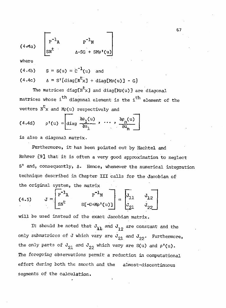
67

(4 4a) p-SN A-SG + SMp'(u)

where

(4.4b) S = S(u) = C-l(u) and

(4.4c) A = S'fdiag[Ntx] + diag[Mp(u)] - G}

The matrices diag[Ntx] and diag[Mp(u)] are diagonal

matrices whose ith diagonal element is the ith element of the

vectors Ntx and Mp(u) respectively and

S(u) apn(u)(4.4d) p'(u) = dag pu, ***

is also a diagonal matrix.

Furthermore, it has been pointed out by Hachtel and

Rohrer [91 that it is often a very good approximation to neglect

S' and, consequently, A. Hence, whenever the numerical integration

technique described in Chapter III calls for the Jacobian of

the original system, the matrix

(4.5) J= =[11 ]2

will be used instead of the exact Jacobian matrix.

It should be noted that J11 and J12 are constant and the

only submatrices of J which vary are J2 1 and J2 2. Furthermore,

the only parts of J21 and J22 which vary are S(u) and p'(u).

The foregoing observations permit a reduction in computational

effort during both the smooth and the almost-discontinuous

segments of the calculation.

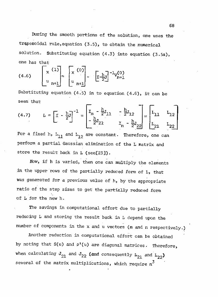
68

During the smooth portions of the solution, one uses the

trapezoidal rule,equation (3.5), to obtain the numerical

solution. Substituting equation (4.3) into equation (3.5a),

one has that

(1) x(0)(4.6) _ % -V (+1

n+l n+l

Substituting equation (4.5) in to equation (4.6), it can be

seen that

(4.7) L = 4 - 2i ' 11 2 2 11 L12

"21 IL-L L

For a fixed h, Ll and L12 are constant. Therefore, one can

perform a partial Gaussian elimination of the L matrix and

store the result back in L (see[23]).

Now, if h is varied, then one can multiply the elements

in the upper rows of the partially reduced form of L, that

was generated for a previous value of h, by the appropriate

ratio of the step sizes to get the partially reduced form

of L for the new h.

The savings in computational effort due to partially

reducing L and storing the result back in L depend upon the

number of components in the x and u vectors (m and n respectively.)

Another reduction in computational effort can be obtained

by noting that S(u) and p'(u) are diagonal matrices. Therefore,

when calculating J21 and J22 (and consequently L21 and L22)several of the matrix multiplications, which require n3

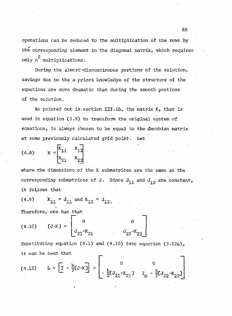
69

operations can be reduced to the multiplication of the rows by

the corresponding element in the diagonal matrix, which requires

only n2 multiplications.

During the almost-discontinuous portions of the solution,

savings due to the a priori knowledge of the structure of the

equations are more dramatic than during the smooth portions

of the solution.

As pointed out in section III.lb, the matrix K, that is

used in equation (3.9) to transform the original system of

equations, is always chosen to be equal to the Jacobian matrix

at some previously calculated grid point. Let

(4.8) K =[

where the dimensions of the K submatrices are the same as the

corresponding submatrices of J. Since Jll and J12 are constant,

it follows that

(4.9) K11 = J1 1 and K12 = J12.

Therefore, one has that

0 0(4.10) [J-K] =

21-K21 J22-K22

Substituting equation (4.1) and (4.10) into equation (3.12a),

it can be seen that

(4.12) L = I - J-K = h11 2K I I hJ _K2 21 21 n 2 22 22

70

Consequently, the use of the transformation, equation (3.9),

effectively yields a system where the first m rows of L are

already reduced --i.e., the first m rows do not require

further Gaussian eliminations.

2. Detection of Smooth and Almost-Discontinuous Segments

As indicated in section III.4, an a priori knowledge

of the nature of the solution can be useful for detecting

whether a smooth or almost-discontinuous segment is being

calculated. As indicated earlier (section IV.1), the smooth

segments are characterized by x and u both changing at about

the same rate and the almost-discontinuous segments are charact-

erized by a very rapid change in u while x remains almost

constant.

If we letm

(4.13a) lAx! IAxiImi=l

and

(4.13b) 11Au 1 I JAu.Jn i=1

then a possible criterion for deciding which segment of

the solution is being calculated can be based on the ratio

(4.14a) R =

as follows:

(1) if the smooth portion is being calculated, then

71

it will be assumed that the smooth portion is still

being calculated if

(4.14b) R > 1/16;

otherwise, it will be assumed that the almost-

discontinuous portion has been entered;

and (2) if the almost-discontinuous portion is being

calculated, then it will be assumed that the almost-

discontinuous portion is still being calculated

if

(4.14c) R < 1/8;

otherwise, it will be assumed that the smooth portion

has been entered.

We should note that, as before, the cross-over point is

not the same in both directions. This is intentional and is

meant to prevent the numerical technique from oscillating back

and forth between the two phases of the integration scheme.

This criterion is also related to the criterion for separating

the two portions that was suggested by [18].

As before, it will be assumed that the initial point

is in the almost-discontinuous section unless otherwise

noted. Also, the initial step size will be set at 1/16th

the maximum step size in order to prevent too many iterations

from being done to solve the implicit equations.

It is suggested by the present author that the new technique

for integrating the almost-discontinuous segments be used if

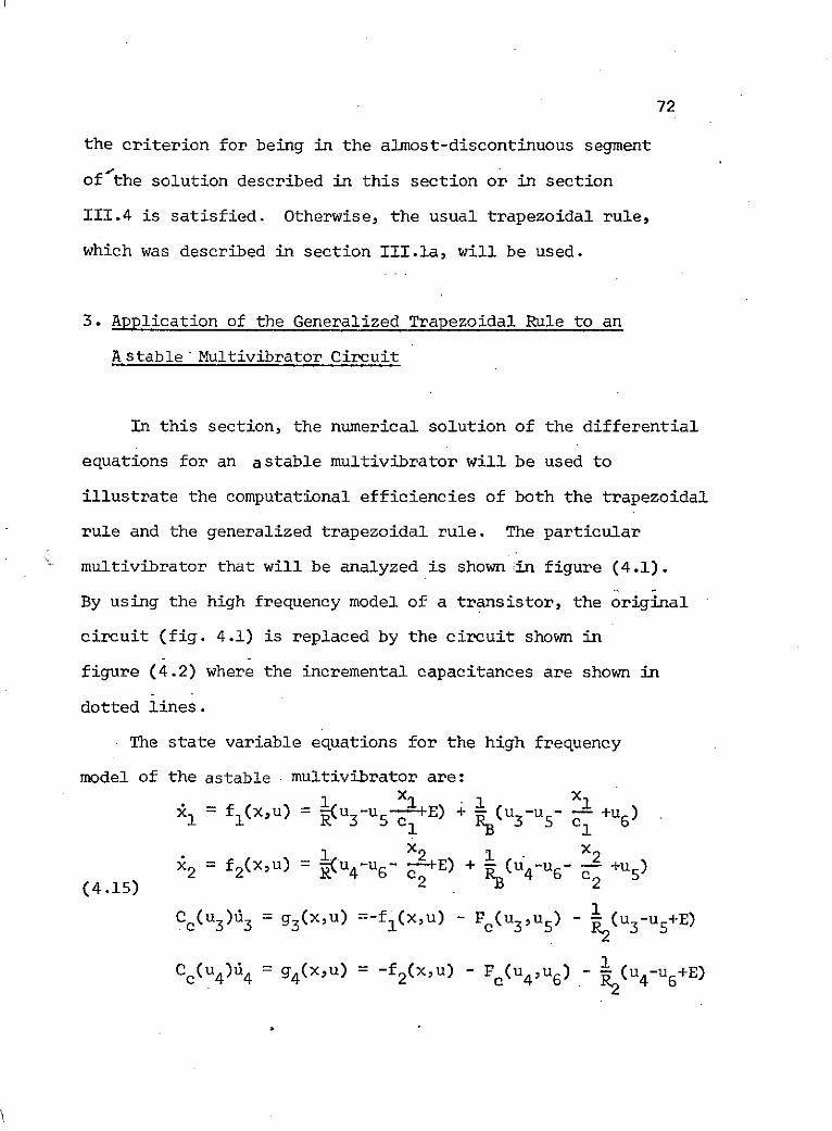
72

the criterion for being in the almost-discontinuous segment

of the solution described in this section or in section

I1.4 is satisfied. Otherwise, the usual trapezoidal rule,

which was described in section III.la, will be used.

3. Application of the Generalized Trapezoidal Rule to an

A stable Multivibrator Circuit

In this section, the numerical solution of the differential

equations for an a stable multivibrator will be used to

illustrate the computational efficiencies of both the trapezoidal

rule and the generalized trapezoidal rule. The particular

multivibrator that will be analyzed is shown in figure (4.1).

By using the high frequency model of a transistor, the original

circuit (fig. 4.1) is replaced by the circuit shown in

figure (4.2) where the incremental capacitances are shown in

dotted lines.

The state variable equations for the high frequency

model of the astable multivibrator are:1 X 1 X

f (x,u) = (u3-u5- - E) + (u-u- u61 5 c1 1 (U3 5 1x x

2 f 2 (x,u) = u4 -u 6 -2+E) + 1 ( u 4 - u +u

(4.15) 2 RB 2

Cc(u3)d3 = 93(x,u) =-fl(x,u) - Fc(u 3 ,u5 ) - (u 3 -u5+E)

Cc(u4 ), 4 g4(x,u) = -f2(x,u)- Fc(u4 ,u6) 1R(u 4-u 6+E)

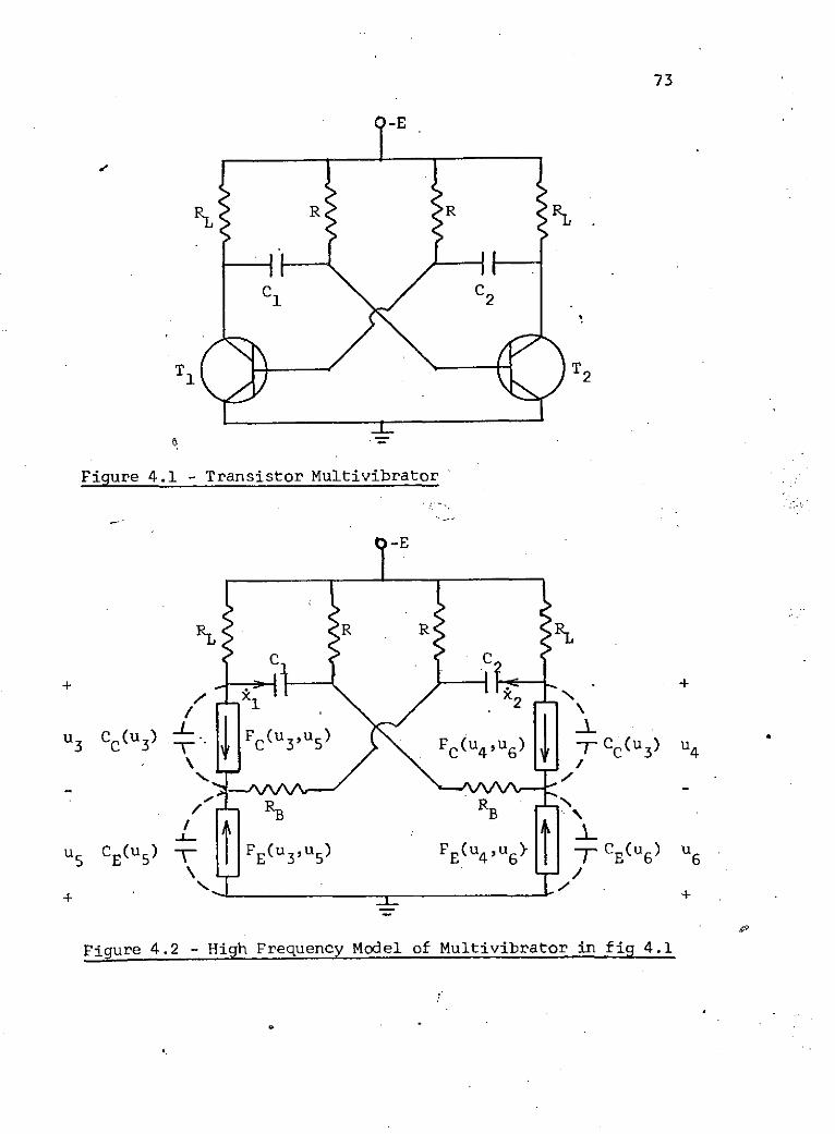
73

-E

RL R R RL

C 1 C2

T1 T2

Figure 4.1 - Transistor Multivibrator

-E

RL R R

Cl C

+ +/ x22(

U3 CC(U 3 Fc( 3 ,u5 (u4 u6 ) CC(u 3) U4

/ RB

u 5 CE(U 5) ~ FE(U 3 u 5 FE(U 4 ,U6) TCE(u6 ) u 6

+ re4.2 - Hih Freuency Model of Multivibato in fi +4.1

Figure 4.2 - High Frequency Model of Multivibrator in fig 4.1

74'

CE(U5)u 5 = g5(x,u) = fl(x,u) - PE(U3 ,u5)1 x2 1

+ (c2 -u4-u5+u6) + (u3 -u 5 +E)

(4.15)cont. CE(u6)d 6 =. 6 (x,u) = f2 (x,u) - FE(U4,u6)

+ Xl -u 3 -u 6 +u 5 ) + 1(Uu6+E)

where

C (u) = CE(u ) = 4X10-4e 4 0u + 2 pF

40V 40Vc(V,VE) = 10[-52(e C-1) - 0.98(e 40VE)]mA

40V_ -40VFE(Vc,VE) = 10- 5[0.98(e C-l) + (e E-1)] mA

(4.16) RB = 0.2 Kx

RL = 0.6 K-r (Units: volts, mA, .Ka,pF)

R= 6. Ka

E = 10 volts

C1 2 = C (varied) pF

The variables xl and x2 are the charges on the capacitors

C1 and C2 respectively, and u3, u4, u5 , and u6 represent

voltages within the transistor model (see figure 4.2).

If one writes equation (4.3) as

(4.17) [1 + R(u) + T(t)

where

(4.18) Q = -, 1C-1Nt -C "G-

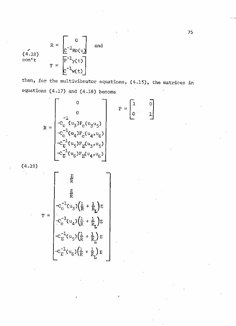
75

R = and

(4.18)con't p- (t)

T =

the - w(t)

then, for the multivibrator equations, (4.15), the matrices in

equations (4.17) and (4.18) become

0 1 0P=

0 0-1

R= -C (3 )Fc(U3U 5)-1

-c (u 4 ) F (u 4 , u 6 )

-1-CE (u 5) E(u 3 , u 5)-1

-CE (uG) E(U 4 ,u 6)

(4.19)

ER

ER

-C1 (u5 + E

-1 1 1

-C (u )(1 + -L EE 5 R

-1 ( 1 )I 1 )E

LE (u6 \R R

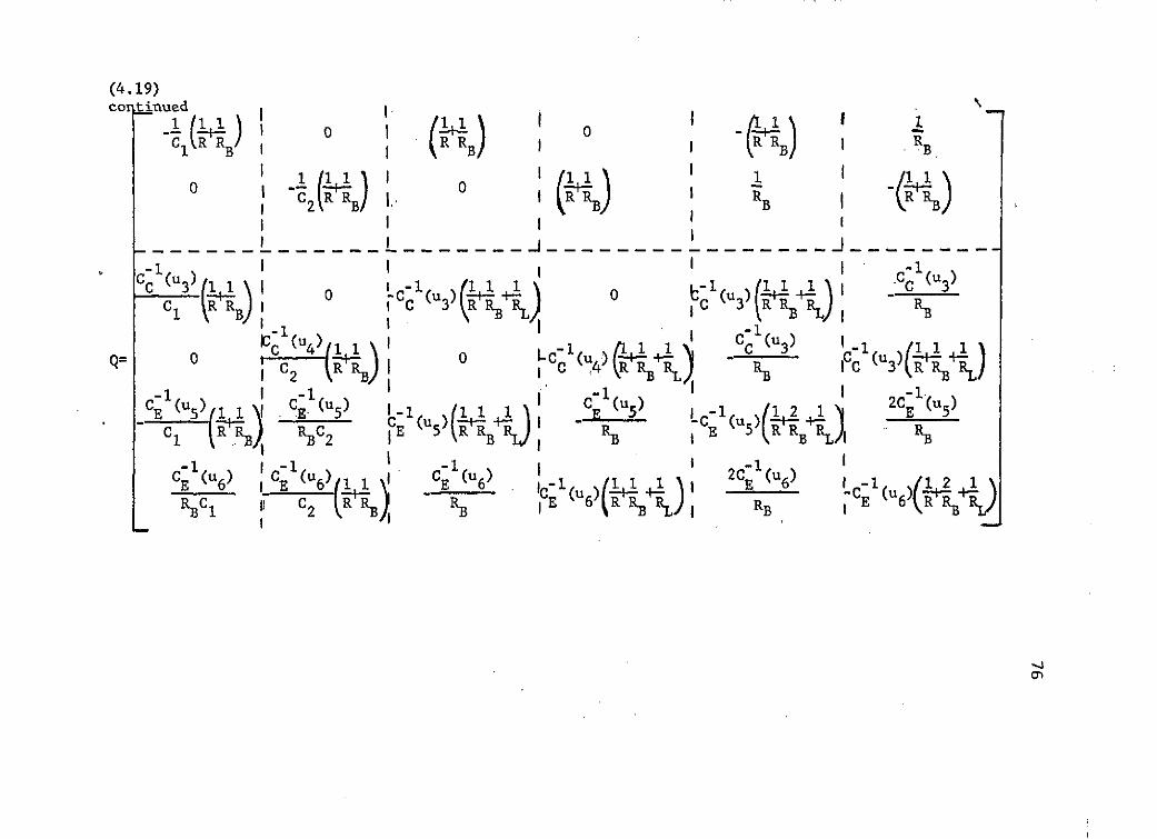
(4.19)co tinued

1 Rm) I R I B

R R I R R RB I

CI- I I I .0C c ( u 3Cik) C. iRIRR RBSo-1

C= (u 2 C o (u

0 2 i B

CE1C ((u U) CE (u B CC (u 3 ) - 2C I u5

R-1 -1 1( - 1

CB I 6) ) () EB C(

CE (6) C (U) c U )2C (g) 1 .0 '

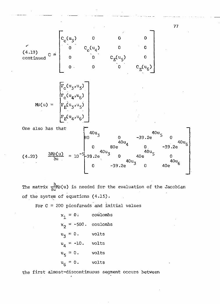
77

Cc(u 3 ) 0 0 0

0 Cc(u 4 ) 0 0(4.19)continued 0 0 CE(U5) 0

0. 0 0 CE(u6

Fc(u 3 ,u5)

Fc (u 4 ,u 6 )

Mp(u) = FE(u 3 ,U 5 )

FE(u4 ,u6)

One also has that40u 40u

0 0 -39.2e 040u 4 40u 6

0 80e 0 -39.2e40u3 40u 5

(4.20) MP = 10- -39.2e 0 40e 0au 40u 40u0 -39.2e 0 40e

The matrix -Mp(u) is needed for the evaluation of the Jacobianau

of the system of equations (4.15).

For C = 200 picofarads and initial values

x = 0. coulombs

X2 = -500. coulombs

u3 = 0. volts

u4 = -10. volts

u5 = 0. volts

u6 = 0. volts

the first almost-discontinuous segment occurs between

78

approximately t = 0 nanoseconds and t = 3 ns. The "correct"

solution at t = 3 ns was obtained by applying global extra-

polation to the solutions that were calculated by means of

the trapezoidal rule with step sizes of 1/512 ns and 1/1024

ns.

In the tables below, the tabulated relative error in

each variable (difference between the calculated and "correct"

solution divided by the "correct" solution for each variable)

in the solution were calculated by means of the generalized

trapezoidal rule and the trapezoidal rule for various maximum

step sizes. The exponential functions needed for the general-

ized trapezoidal rule were evaluated by means of the E22

Pade approximation with s = 4.

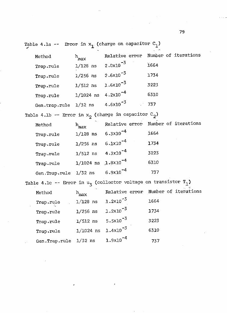
79

Table 4.1a -- Error in xl (charge on capacitor C1)

Method h Relative error Number of iterationsmax

-3Trap.rule 1/128 ns 2.0x10-3 1664

Trap.rule 1/256 ns 2.6xl0-3 1734

Trap.rule 1/512 ns 1.6X10-3 3223-4

Trap.rule 1/1024 ns 4.2x10 6310-3

Gen.trap.rule 1/32 ns 4.6x10 737

Table 4.1b -- Error in x2 (charge in capacitor C2)

Method h Relative error Number of iterationsmax

-4Trap.rule 1/128 ns 6.3x0 -4 1664

-4Trap.rule 1/256 ns 6.110-4 1734

-4Trap.rule 1/512 ns 4.3xl0-4 3223

Trap.rule 1/1024 ns .8X10-4 6310

Gen.Trap.rule 1/32 ns 6.9X10 -4 737

Table 4.1l -- Error in u3 (collector voltage on transistor TI)

Method hmax Relative error Number of iterations-3

Trap.rule 1/128 ns 1.2X10 1664-3

Trap.rule 1/256 ns 1.2X10 1734

-3Trap.rule 1/512 ns 5.5x10 - 3 3223

Trap.rule 1/1024 ns 1.4x10-3 6310

Gen.Trap.rule 1/32 ns 1.9x10-4 737

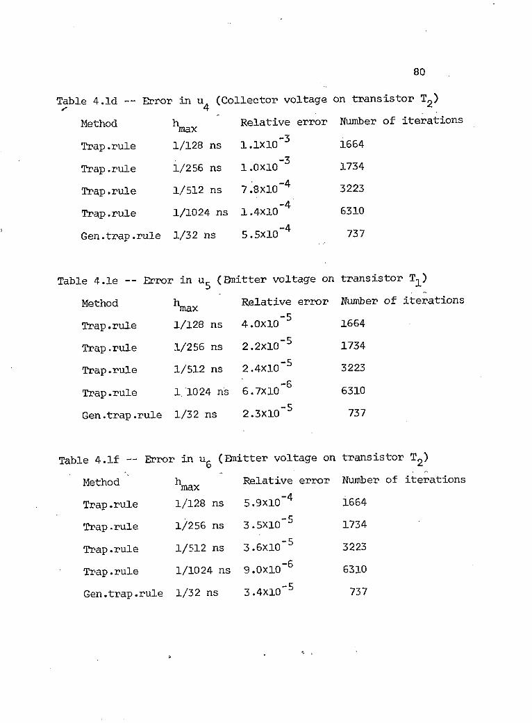
80

Table 4.1d -- Error in u (Collector voltage on transistor T2)

Method h Relative error Number of iterationsmax

-3Trap.rule 1/128 ns l.lXl0-3 1664

-3Trap.rule 1/256 ns 1.Oxl0-3 1734

Trap.rule 1/512 ns 7.8x10 - 4 3223-4

Trap.rule 1/1024 ns 1.4x10-4 6310

Gen.trap.rule 1/32 ns 5.5x10-4 737

Table 4.le -- Error in u5 (mitter voltage on transistor T1)

Method hmax Relative error Number of iterations-5

Trap.rule 1/128 ns 4.010- 1664

Trap.rule 1/256 ns 2.2x10-5 1734

Trap.rule 1/512 ns 2.4x10-5 3223

-6Trap.rule 1,1024 ns 6.7x10 6310

-5Gen.trap.rule 1/32 ns 2.3x10 5 737

Table 4.1f -- Error in u6 (DEitter voltage on transistor T2 )

Method h Relative error Number of iterationsmax

Trap.rule 1/128 ns 5.9x10-4 1664

-5Trap.rule 1/256 ns 3.5X10-5 1734

Trap.rule 1/512 ns 3.6X10 -5 3223-6

Trap.rule 1/1024 ns 9.0x10-6 6310

Gen.trap.rule 1/32 ns 3.4X10 -5 737

81

From the above tables, it can be seen that the generalized

trapezoidal rule with a maximum step size of 1/32 ns

produced a solution whose error was less than the error for

the trapezoidal rule with a step size of 1/512 ns but not as

accurate as the latter with a step size of 1/1024 ns.

Moreover, the generalized trapezoidal rule required approx-

imately 1/5 as many iterations over the interval t = 0 to

t = 3 ns as did the trapezoidal rule with h = 1/512 ns.

As was the case with the third example in section 111.5,

for a given hmax the generalized trapezoidal rule and the

trapezoidal rule produced solutions with approximately the

same accuracy for the "slow" variables (xl and x2 ), but the

generalized trapezoidal rule produces more accurate solutions

for the "fast" variables (u3 , u4 , u5, and u6).

82

V. Conclusions and Suggestions for Further Research.

1. Conclusions

The research reported herein developed a new numerical

integration technique for solving stiff systems of ordinary

differential equations. The method, which is called the

generalized trapezoidal rule, is a modification of the trap-

ezoidal rule. However, the new method is computationally more

efficient than the trapezoidal rule when the solution of the

almost-discontinuous segments is being computed.

The computation of the solution of the system of ordinary

differential equations is divided into two parts. For the

computation of the smooth segments of the solution, the trap-

ezoidal rule with Newton-Raphson iterations to solve the

implicit equations is used. However, during the almost-

discontinuous segments, the generalized trapezoidal rule with

both Newton-Raphson and modified Newton-Raphson iterations

to solve the implicit equations is used to calculate the

solution. The details of the computation for both types of

segments is found in sections III.la and III.1b.

As pointed out in section 111.4, the detection of whether

one is calculating a smooth or an almost-discontinuous segment

is at best a difficult task. The detection method based on

the step size chosen by the integration scheme that was used

83

in the research presented herein can be hazardous if the user

has specified a "very large" maximum step size, hma It is

hazardous in the sense that the integration procedure might

choose the generalized trapezoidal rule instead of the trap-

ezoidal rule during the smooth segments. However, during the

smooth segments, the generalized trapezoidal rule is not as

computationally efficient as the trapezoidal rule. For a given

step size, both the trapezoidal rule and the generalized

trapezoidal rule produce solutions with approximately the same

accuracy. Since the generalized trapezoidal rule requires

more work per step than the trapezoidal rule, the latter should

be used for the calculation of smooth segments of the solution.

Therefore, care must be taken not to specify a value for

hmax that will be much larger than the step size chosen by

the step size control procedure used with the trapezoidal rule.

If the user does not have experience in choosing a proper

maximum step size for a particular problem, he should do some

preliminary calculations with the trapezoidal rule and observe

the step sizes selected.

The results discussed in sections 111.3 (Theoretical

Error Calculations), 11.5 (Illustrative Computer Results),

and IV.3 (Computational Results for a Multivibrator Circuit)

indicate that the generalized trapezoidal rule is computation-

ally more efficient than the trapezoidal rule for computing

the solution during an almost-discontinuous segment of the

84

solution. That is, the generalized trapezoidal rule enables

Ohe to use larger step sizes and to do fewer iterations to

solve the implicit integrating equations during the almost-

discontinuous segments than the trapezoidal rule while

maintaining the same or improved accuracy as compared to

the trapezoidal rule. Also, the numerical solution produced

by the generalized trapezoidal rule did not have an oscillatory

behavior at step sizes for which the trapezoidal rule

produced an oscillating solution (even though the actual solution

was decaying exponentially).

The generalized trapezoidal rule is not meant for obtain-

ing very fine detailed solutions during the almost-discontinuous

segments. The basic aim of the scheme is to take larger

time steps than is possible with the trapezoidal rule while

maintaining a predetermined accuracy in the solution.

Consequently, if one needs very fine details of the solution

during the almost-discontinuous segments, the trapezoidal

rule, or perhaps step length limited schemes such as explicit

Runge-Kutta methods should be used instead of the generalized

trapezoidal rule.

From the foregoing remarks and the results of the previous

chapters, it may be concluded that for stiff systems of

ordinary differential equations even though the generalized

trapezoidal rule requires more work per iteration than the

trapezoidal rule, the overall computational effort needed

to compute the almost-discontinuous segment of the solution

85

is less for the generalized trapezoidal rule.

2. Sugqestions for Further Research

The research presented herein suggests several important

questions that should be pursued further. The applicability

of an exponential shift in variables to other A-stable

schemes should considered. Of particular interest would

be the effects of the transformation on the concept of

exponential fitting [17], and on the implicit midpoint

scheme [22].

One would like to know whether the exponential trans-

formation would improve the computational efficiency of

exponential fitting. The exponential transformation has

a tendency to compress the eigenvalues, especially the

larger ones; whereas, the exponential fitting method tries

to approximate the decay of the larger eigenvalues. It

is not clear how a combination of the two ideas would

perform in terms of computational efficiency.

The implicit midpoint scheme is closely related to the

trapezoidal rule and it is quite likely that exponential

time shifts would improve the computational efficiency in

about the same way that the transformation improves the

efficiency of the trapezoidal rule. However, this remains to

be demonstrated.

86

The application of the exponential transformation to

the stiffly stable multi-order scheme of Gear [8] is also

of considerable interest. The compressing effect on the

eigenvalues of the exponential transformation might alleviate

the problem of poorly situated eigenvalues (see section 11.8).

Also, it would be interesting to note the effect of the

transformation on the order of the scheme selected by the

automatic procedure.

A third direction for further research is to find the

effect of the transformation on the h2 nature of the error

expansion for the trapezoidal rule. The fact that the

error terms for the trapezoidal rule can be expressed in

powers of h2 allows for a great increase in the computational

efficiency of global extrapolation. Thus, the question to

be examined is how the exact exponential transformation

and the various Pade approximations (inconjunction with the

usual argument reduction scheme) change the basic form of

the error expansions for the trapezoidal rule.

87

VI. References

[13 G. Bjurel, G. Dahlquist, B. Lindberg, S. Linde & L. Oden,"Survey of Stiff Ordinary Differential Equations,"Report NA 70.11 Department of Computer Science, RoyalInstitute of Technology, Stockholm, Sweden

[2] J.C. Butcher, "Implicit Runge-Kutta Processes," Mathematicsof Computation, 18, (1964),#85, pp50-64

[3] G. Dahlquist, "A Special Stability Problem for LinearMultistep Methods," BIT (Nordisk Tidskrift for Information-behandling) 3, (1963), pp 27-43

[4] G. Dahlquist, "Stability Questions for Some NumericalMethods for Ordinary Differential Equations," Proceedingsof the Symposium of Applied Mathematics, 15 , (1963)

[5] G. Dahlquist and B. Lindberg, Private communications (1971)

[6] B. Ehle, "The Application of Implicit Runge-Kutta Processesto Stiff Systems," Research Report CSRR 2007, Universityof Waterloo, Waterloo, Ontario, Canada

[7] M. Fowler & R. Warten, "A Numerical Integration Techniquefor Ordinary Differential Equations with Widely SeparatedEigenvalues," IBM Journal of Research and Development,September 1967, pp 537-543

[8] C.Gear, "The Automatic Integration of Stiff OrdinaryDifferential Equations," IFIPS Conference 1968 (Edinburgh,Scotland)

[9] G. D. Hachtel & R. A. Rohrer, "Techniques for OptimalDesign and Synthesis of Switching Circuits," Proceedingsof the' IEEE, 55, #11, (November 1967), pp 1864-1877

[10] P. Henrici, Discrete Variable Methods in OrdinaryDifferential Equations, J. Wiley & Sons, (1962)

[11] P. Henrici, Error Propagation for Difference Methods,J. Wiley & Sons, (1964)

[12] T. E. Hull, "The Numerical Integration of OrdinaryDifferential Equations," IFIPS Congress 1968 (Edinburgh,Scotland)

[13] J. D. Lawson, "Generalized Runge-Kutta Processes forStable Systems with Large Lipschitz Constants," SIAMJournal of Numerical Analysis, 4, (1967), #3, pp 372-380

88

[14] L. Lapidus & J. Seinfeld, Numerical Solution of OrdinaryDifferential Equations, Academic Press (1971)

[15] B. Lindberg, "On Smoothing and Extrapolation for theTrapezoidal Rule," BIT, 11, (1971), pp29-52

[16] W. Liniger, "A Stopping Criterion for the Newton-RaphsonMethod in Implicit Multistep Integration Algorithmsfor Nonlinear Systems of Ordinary Differential Equations,"Communications of the ACM, 14,#9, (September 1971),pp 600-601

[17] W. Liniger & R. Willoughby, "Efficient Numerical Integrationof Stiff Systems of Ordinary Differential Equations,"IBM Research Report RC 1970 (December 1970)

[18] S. J. Oh, T. E. Stern & H. E. Meadows, "On the Analysis ofNon-Linear Irregular -Networks," Symposium on GeneralizedNetworks, Polytechnic Institute of Brooklyn, April 1966

[19] J. Rosenbaum, "Pade Approximations to the ExponentialFunctions Exp (-z) and Exp (-At), " Technical Memorandum,Department of Electrical Engineering, Columbia University,(December 1969)

[20] T. E. Stern, "Computer Aided Analysis of Non-LinearNetworks," Systems Research Group, Technical Report# 107, Department of Electrical Engineering, ColumbiaUniversity, ( July 1968)

[21] T. Stern, "Efficient Computer Aided Analysis of Non-Linear Semiconductor Networks," IEEE Mexico Conference(January 1971)

[22] H. J. Stetter, Private communication through G. Dahlquist(1971)'

[23] W. Tinney & J. Walker, "Direct Solution of SparseNetwork Equations by Optimally Ordered TriangularFactorization," Proceedings of the IEEE, 55,#11,(November 1967) pp 1801-1809

[24] O. Widlund, "A Note on Unconditionally Stable LinearMultistep Methods," BIT, 7, (1967), pp 65-70

[25] R. S. Varga, Matrix Iterative Analysis, Prentice Hall(1962)

[26] F. H. Branin, Jr., Private communications (1971)

[271 C. Gear, Private communications (1971)

89

[28] J. Millman and H. Taub, Pulse Digital and SwitchingWaveforms, McGraw Hill ( 1965)

90

VIT. Appendix

On the next several pages there is a listing of the PL/I

program used to calculate the results reported herein.

The program is set up for a maximum of 6 equations; but the

declaration statements can easily be changed to accomodate

any other number of equations.

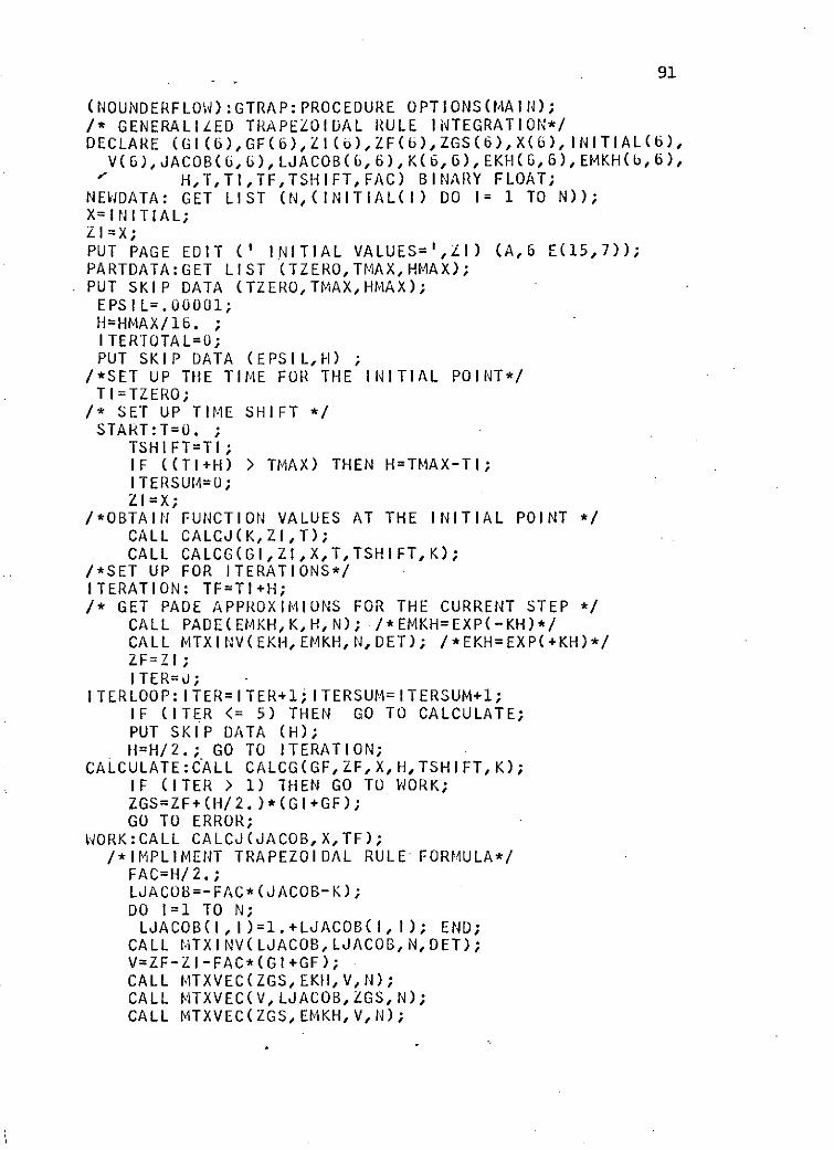
91

(NOUNDERFLOW):GTRAP:PROCEDURE OPTIONS(MAIN);/* GENERALIZED TRAPEZOIDAL RULE INTEGRATION*/DECLARE (GI (6),GF(6),ZI(b),ZF(t ),ZGS(6),X(6), INITIAL(6),

V(6),JACOB(6,6),LJACOB(6,6),K(6,6),EKH(6,6),EMKH(b,6),' H,T,TI,TF,TSHIFTFAC) BINARY FLOAT;

NEWDATA: GET LIST (tI,(INITIAL(I) DO I= 1 TO N));X=INITIAL;ZI=X;PUT PAGE EDIT (' INITIAL VALUES=',ZI) (A,6 E(15,7));PARTDATA:GET LIST (TZERO,TMAX,HMAX);PUT SKIP DATA (TZERO,TMAX,HMAX);EPSIL = .00001;H=HMAX/16. ;I TERTOTAL=0;PUT SKIP DATA (EPSIL,H) ;

/*SET UP THE TIME FOR THE INITIAL POINT*/TI=TZERO;

/* SET UP TIME SHIFT */START:T=O. ;

TSHIFT=TI;IF ((TI+H) > TMAX) THEN H=TMAX-TI;ITERSUM=O;ZI=X;

/*OBTAIN FUNCTION VALUES AT THE INITIAL POINT */CALL CALCJ(K,ZI,T);CALL CALCG(GI,ZI,X,T,TSHI FT,K);

/*SET UP FOR ITERATIONS*/ITERATION: TF=TI+H;/* GET PADE APPROXIMIONS FOR THE CURRENT STEP */

CALL PADE(EMKH,K,H,N); /*EMKH=EXP(-KH)*/CALL MTXINV(EKH,EMKH,N,DET); /*EKH=EXP(+KH)*/ZF=ZI;ITER=J;

ITERLOOP:ITER=ITER+1;ITERSUM=ITERSUM+1;IF (ITER <= 5) THEN GO TO CALCULATE;PUT SKIP DATA (H);H=H/2.; GO TO ITERATION;

CALCULATE:CALL CALCG(GF,ZF,X,H,TSHIFT,K);IF (ITER > 1) THEN GO TO WORK;ZGS=ZF+(H/2. )*(GI+GF);GO TO ERROR;

WORK:CALL CALCJ(JACOB,X,TF);/*IMPLIMENT TRAPEZOIDAL RULE FORMULA*/

FAC=H/2.;LJACOB=-FAC* (JACOB-K);DO 1=1 TO N;LJACOB(I,I)=1.+LJACOB(I,I); END;

CALL MITX INV(L J ACOB, LJACOB, N, DET);V=ZF-ZI-FAC*(GI+GF);CALL MTXVEC(ZGS,EKH,V,N);CALL IMTXVEC(V,LJACOB,ZGS,N);CALL MTXVEC(ZGS,EMKH,V,N);

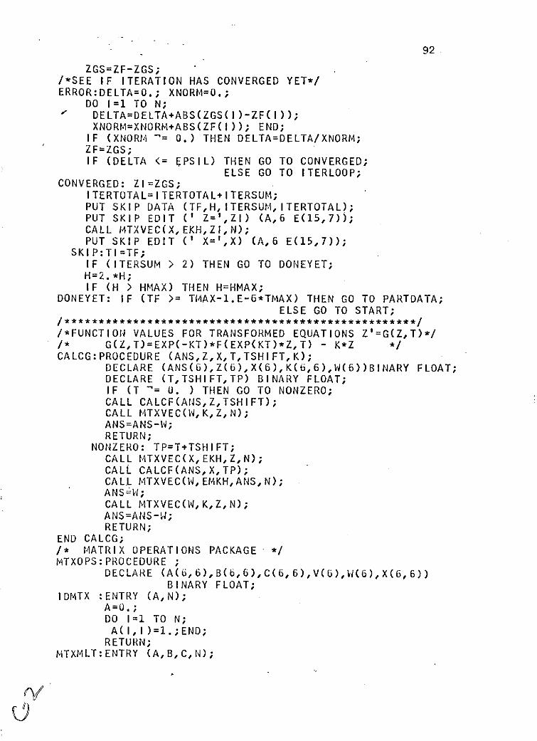
92

ZGS=ZF-ZGS;/*SEE IF ITERATION HAS CONVERGED YET*/ERROR:DELTA=O.; XNORM=O.;

DO I=1 TO N;" DELTA=DELTA+ABS(ZGS(I)-ZF( I));

XNORM=XNORM+ABS(ZF(I)); END;IF (XNORM '= 0.) THEN DELTA=DELTA/XNORM;ZF=ZGS;IF (DELTA <= EPSIL) THEN GO TO CONVERGED;

ELSE GO TO ITERLOOP;CONVERGED: ZI=ZGS;

ITERTOTAL=ITERTOTAL+I TERSUM;PUT SKIP DATA (TF,H,ITERSUM,ITERTOTAL);PUT SKIP EDIT (' Z=',ZI) (A,6 E(15,7));CALL M1TXVEC(X,EKH,ZI,N);PUT SKIP EDIT (' X=',X) (A,6 E(15,7));

SKIP:TI=TF;IF (ITERSUM > 2) THEN GO TO DONEYET;H=2.*H;IF (H > HMAX) THEN H=HMAX;

DONEYET: IF (TF >= TMAX-1.E-6*TMAX) THEN GO TO PARTDATA;ELSE GO TO START;

/***************************************************/

/*FUNCTION VALUES FOR TRANSFORMED EQUATIONS Z'=G(ZT)*//* G(Z,T)=EXP(-KT)*F(EXP(KT)*ZT) - K*Z */CALCG:PROCEDURE (ANS,Z,X,T,TSHIFT,K);

DECLARE (ANS(6),Z(6),X(6),K(6,6),W(6))BINARY FLOAT;DECLARE (T,TSHIFT,TP) BINARY FLOAT;IF (T "= U. ) THEN GO TO NONZERO;CALL CALCF(ANS,Z,TSHIFT);CALL MTXVEC(W,K,Z,N);ANS=ANS-W;RETURN;

NONZERO: TP=T+TSHIFT;CALL MTXVEC(X,EKH,Z,N);CALL CALCF(ANS,X,TP);CALL MTXVEC(W,EMKH,ANS,N);ANS- W;CALL MTXVEC(W,K,Z,N);ANS=ANS-W;RETURN;

END CALCG;/* MATRIX OPERATIONS PACKAGE */MTXOPS:PROCEDURE ;

DECLARE (A(6,6),B(6,6),C(6,6),V(6),W(6),X(6,6))BINARY FLOAT;

IDMTX :ENTRY (A,N);A=O.;DO I=1 TO N;A(1,1)=1.;END;

RETURN;MTXMLT:ENTRY (A,B,C,N);

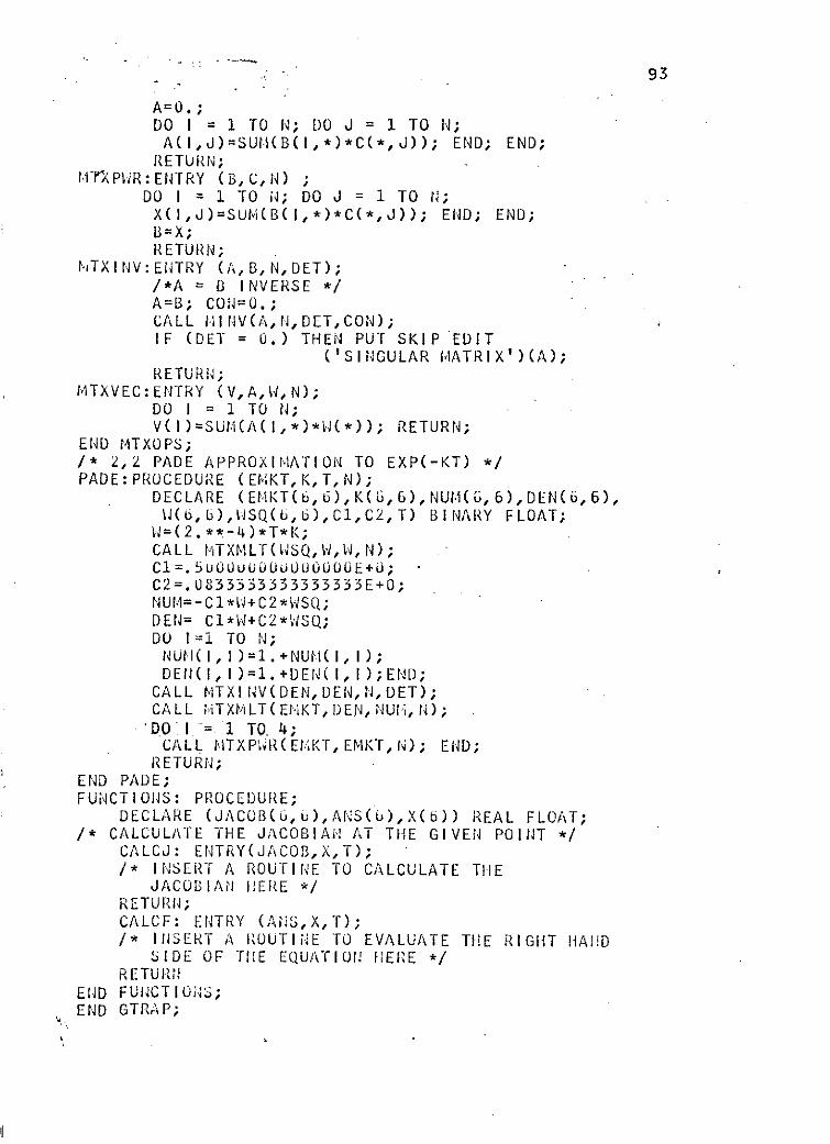
93

A=0.;DO I = 1 TO N; DO J = 1 TO N;A(I,J)=SUH(B(I,*)*C(*,J)); END; END;RETURN;

['1XPWR: ENTRY (B, C, N) ;DO I = 1 TO N; DO J = 1 TO N;X(I,J)=SUM(B(I,*)*C(*,J)); END; END;B=X;RETURN;

hTXINV:ENTRY (A,B,N,DET);/*A = B INVERSE */A=B; CON=O.;CALL MINV(A,N,DET,CON);IF (DET = 0.) THEN PUT SKIP EDIT

('SINGULAR MATRIX')(A);RETURN;

MTXVEC:ENTRY (V,A,W,N);DO I = 1 TO N;V(1)=SUM(A(I,*)*W(*)); RETURN;

END MTXOPS;/* 2,2 PADE APPROXIIATION TO EXP(-KT) */PADE:PROCEDURE (EEMKT,K,T,N);

DECLARE (EMKT(6,6),K(, 6),NUM(G, 6),DEN(6, 6),W(6,b),WSQ(,6),C1,C2,T) BINARY FLOAT;W=(2.**-4)*T*K;CALL MTXMLT(WSQ,W,W,N);C1=.5UUOuuU0Uu00U0E+O;C2= .0833333333333333E+O;NUM = -C1*W+C2*WSQ;DEN = C1*W+C2*WSQ;DO 1=1 TO N;NU.(I, I)=1.+NUH(I, I);DEN(I, I)=1.+DEN(1,1);END;

CALL MTXINV(DEN,DEN,N,DET);CALL HTXMLT(EIiKT, DEN, NUfi,N);'DO I -= 1 TO 4;

CALL HTXPWR(EIKT, EMKT,N); END;RETURN;

END PADE;FUNCTIONS: PROCEDURE;

DECLARE (JACOB(G,6),ANS(b),X(6)) REAL FLOAT;/* CALCULATE THE JACOBIAN AT THE GIVEN POINT */

CALCJ: ENTRY(JACOB,X,T);/* INSERT A ROUTINE TO CALCULATE THE

JACOBIAN HERE */RETURN;CALCF: .ENTRY (ANS,X,T);/* INSERT A ROUTINE TO EVALUATE THE RIGHT HA!D

SIDE OF TIE EQUATION HERE */RETURN

END FUNCTIONS;END GTRAP;