Claremont CollegesScholarship @ Claremont

CMC Senior Theses CMC Student Scholarship

2015

Player Compensation and Team Performance:Salary Cap Allocation Strategies across the NFLMax WinsbergClaremont McKenna College

This Open Access Senior Thesis is brought to you by Scholarship@Claremont. It has been accepted for inclusion in this collection by an authorizedadministrator. For more information, please contact scholarship@cuc.claremont.edu.

Recommended CitationWinsberg, Max, "Player Compensation and Team Performance: Salary Cap Allocation Strategies across the NFL" (2015). CMC SeniorTheses. Paper 1006.http://scholarship.claremont.edu/cmc_theses/1006

CLAREMONT MCKENNA COLLEGE

Player Compensation and Team Performance: Salary Cap Allocation Strategies across the NFL

SUBMITTED TO

PROFESSOR JOSHUA ROSETT

AND

DEAN NICHOLAS WARNER

BY

MAX WINSBERG

FOR

SENIOR THESIS

FALL 2014

DECEMBER 1, 2014

Table of Contents Abstract…………………………………………………………………………....1 Introduction………………………………………………………………………..2 The History of the NFL Salary Cap……………………………………………….3 Literature Review………………………………………………………………….5 The Model………………………………………………………………………..10 Selection of Variables……………………………………………………………14 Data……………………………………………………………………………....15 Results……………………………………………………………………………16 Summary and Conclusion ……………………………………………………….23 Appendix………………………………………………………………………....25 Works Cited……………………………………………………………………...40

Abstract

The National Football League’s salary cap constrains the available resources each

franchise is allotted to spend on player personnel. I examine the effects of executive

management’s compensation allocation strategies on team performance from 2006 to

2013. The findings suggest that spending more than the league-average on offensive

lineman hurts overall team performance. Spending above the league average on both the

offensive line and quarterback positions negatively affects offensive performance as well.

This supports previous research stating that taking a superstar-approach to cap

distribution negatively affects team performance. Furthermore, I find evidence of

increased compensation inequality among players under the Collective Bargaining

Agreement of 2011 compared to that of 1993.

1

I. Introduction

In 1993, the National Football League (“NFL”) and its players’ association agreed

on a collective bargaining agreement (“CBA”) that created a salary cap, or limit, on the

amount of money each franchise is allowed to spend on its players in a particular season.

In exchange for team salary caps, the players received the right to gain free agency for

the first time. Free agency allows players to switch teams upon the expiration of their

contract with their current team. The creation of free agency created a new dynamic in

the sport as it opened the door for franchises to sign players who were previously

unavailable to them.

The combination of both free agency and the NFL salary cap created the need for

franchises to allocate their available resources as efficiently as possible. Teams needed to

find an optimal relationship between player compensation and team performance. This

relationship between compensation and performance is common throughout economics

and finance research. The study of allocating available resources to maximize

performance has been studied at length and is discussed in the literature review in the

ensuing section. The purpose of this study is to determine the potential effect of player

compensation allocation on team performance. The measure of team performance that I

use primarily consists of each team’s number of regular season wins over the duration of

the study (2006-2013).

The paper proceeds in the following order. To conclude Section I, I provide a

brief history on the NFL salary cap and a literature review of previous studies on related

topics. In Section II, a model is supplied to examine the relationship between player

2

compensation and team performance, while Section III, outlines the data and variables

used in the study. I report the results of the study in Section IV and offer possible

explanations for the results produced. Finally, a summary and conclusion are provided in

Section V. This section includes a discussion on further work needed to advance this

preliminary study.

History of the NFL Salary Cap

The NFL instituted a hard salary cap for the 1994 season in accordance with the

1993 CBA between the NFL and the National Football League Players’ Association

(NFLPA). The introduction of the salary cap was designed to create greater parity among

NFL teams and is often credited for the league’s enormous popularity. Under the 1993

CBA, the NFL set the salary cap for each new league year based on a percentage of their

Defined Gross Revenues. In 2006, the formulation was changed to include a percentage

of the NFL’s total salary, which added other revenue streams such as local advertising.

The hard salary cap forbids teams from exceeding the league’s salary cap ceiling

for that specific year.1 A team’s salary cap is the sum of each player’s “cap value” on

their 53-man roster. Player contracts consist of a base salary and various bonuses which

can be earned over the life of the contract. A player’s base salary is not guaranteed,

meaning they can be released at any time during the contract and the team no longer has

the obligation to pay them their base salary. Bonuses, on the other hand, are paid as lump

sums at the date in which they are earned and generally cannot be recovered. The

different type of bonuses include signing bonuses (paid at beginning of contract), training

3

camp bonuses (paid at beginning of training camp), roster bonuses (paid upon making the

53-man roster), and an assortment of incentive bonuses. These incentive bonuses are

distinguished between “likely to be earned” bonuses (LBTEs) and “not likely to be

earned” bonuses (NLBTEs). A player’s cap value is calculated as:

Cap Value = Base salary + (total contract signing bonus/number of seasons of

contract duration) + training camp bonus + roster bonus + LTBEs (1)

As mentioned previously, the sum of each players cap value on the 53-man roster

cannot exceed the league’s salary cap. Table 2 shows the league wide salary cap for the

years 2006-2013, the focus of this research. In 2008, the NFL owners opted out of the

1993 CBA which led to an uncapped year in 2010. The NFL cautioned the 32 teams not

to take advantage of the uncapped year by front-loading contracts in order to have a

reduced cap hit in future capped seasons. Most teams listened and treated the 2010 season

as if there was a cap in place even though nothing was ever put into writing. However,

the Dallas Cowboys and Washington Redskins did not adhere to the advice and severely

front-loaded their contracts during this 2010 season. The NFL retaliated by stripping the

Cowboys of $10 million of cap space and the Redskins of $36 million of cap space over

the 2011 and 2012 seasons. Although neither team technically violated the salary cap, the

penalty remained after appeals from both the franchises. I will include the 2010 season in

my regressions for this study due to 30 of the 32 teams treating the season as if there was

a salary cap in place. However, an altercation may be needed to normalize the effects of

the Cowboys and Redskins generous spending.

4

The NFL and NFLPA agreed to a new CBA in 2011 which reinstated the salary

cap starting in the 2011 season. The 2011 CBA created a $120 million salary cap for the

2011 season and introduced a salary floor that would not be enforced until the 2013

season. The cap floor required each team to spend at least 88.8% of the salary cap in

2013 and 90% thereafter. The salary floor is intended to deter teams from significantly

reducing player contracts in an effort to minimize costs. The cap floor is based on total

cash spent over two separate four year periods allowing teams to spend less than the floor

in certain seasons without violating the CBA.

Literature Review

In 1994, the NFL instituted a salary cap that limits the amount of money a given

team can spend on its roster. The introduction of this hard salary cap resulted from the

new collective bargaining agreement in an effort to create parity across the different

franchises. Larsen, Fenn, and Spenner (2006) confirm the implementation of the salary

cap in the NFL did increase competitive balance by spreading the wealth of talent around

the league. They found that teams’ cap spending from 2000-2002 was negatively

correlated with their spending from 2004-2005. This implies that the salary cap is

effective in reducing teams from constantly spending more than other teams year after

year. With a salary cap and increased parity in the NFL, it is important for teams to

strategically allocate resources across players and positions to maximize wins and

increase return to owners.

5

Kowalewski and Leeds (1999) focus on the distribution and structure of salaries

in the NFL from 1992-1994, before and after the implementation of the salary cap. By

using Gini coefficients, Kowalewski and Leeds conclude that the salary cap created a less

equal distribution of salaries in the NFL. The Gini coefficient, which measures statistical

dispersion of income distribution, rose from 0.393 in 1992 to 0.479 in 1993. The rise in

the Gini coefficient shows a significant increase in the inequality of contracts in the NFL.

Furthermore, Kowalewski and Leeds found that “superstars” received higher pay after the

salary cap in 1994 in relation to the pre- salary cap era in 1992. The increase in salary for

superstars seemed to come at expense of the marginal players in the NFL. Players in the

60th percentile in salary distribution earned less money under the new salary cap rules,

whereas the players at around the 65th percentile earned higher salaries post salary cap.

The increase in salary inequality started to push the “NFL toward a two-class system with

a small group of very wealthy players and a much larger group of (relatively) poor

players” (p.219). The effect of the inequality of pay between the superstars and everyone

else is discussed below on when analyzing team success in relation to resource allocation.

In a later study, Kowalewski and Leeds (2001) dive deeper and look at the effect

of the salary cap on the compensation of offensive skill players in the NFL. Offensive

skill players consist of the players who regularly touch the football such as quarterbacks,

running backs, wide receivers, and tight ends. The authors employ a quantile regression

for players at the 25th and 75th quantiles of income distribution2. This regression allows

them to compare and contrast players that are highly-paid with players that receive lower

levels of income. The results showed that all offensive skill players’ mean salaries rose,

but only quarterbacks’ median salary increased as well. This illustrates that the salaries of

6

running backs, wide receivers, and tight ends became skewed to the right after the

introduction of the salary cap. Unlike their previous study, Kowalewski and Leeds

indicate that it is easier for players in the .25 quantile to increase their wages, while it was

less common for those players that were already compensated well in the .75 quantile.

Intuitively, this makes sense as “a player’s bargaining power from having a good year is

greater when he is relatively underpaid than when he is relatively highly paid” (p.256).

An important factor to consider in the Kowalewski and Leeds findings revolves

around non-guaranteed contracts in the NFL. Franchises can release a player who is not

performing well and not be stuck with his base salary for future years. Teams frequently

sign players to large contracts and release them before the end of the agreement. This can

partially account for why it is less common for players who are already highly paid to

achieve further economic gain. Thus, guaranteed money, often signing bonuses, are a

better indicator of the economic commitment a franchise makes to its players. Signing

bonuses are usually collected in the early years of a contract and must be paid even if the

player is released. Finally, Kowalewski and Leeds observe compensation post-salary cap

is more reliant on performance. This differs with the pre-salary cap era where players

were compensated mainly for which position they played.

Rosen (1981) points out in particular labor markets, even small differences in

talent can cause enormous differences in income distribution. This seems to be the case

with player contracts in the NFL. Rosen labels this the “superstar effect” where “the

income distribution is stretched out in its right-hand tail compared to the distribution of

talent” (p.846). This “superstar effect” can help explain the two-class system that

Kowalewski and Leeds (1999) found in NFL wages.

7

Quinn, Geier, and Berkovitz (2007) delve further into the allocation of teams’

salary cap by analyzing every NFL franchise’s budget from 2000-2005. Their findings

are consistent with Rosen’s “superstar” income distribution and are supported by a

“marginal win utility product” model rather than the standard marginal revenue product

model. This seems accurate because there is not a significant drop off in talent when

comparing the highest paid players down to the lowest paid players. Thus, the “superstar”

income distribution makes sense because small differences in talent results in large pay

inequality due to the large impact on wins of even small difference of talent. In addition,

the authors investigate salary cap distribution among players and on-field results. They

found that teams with a higher than average winning percentage allocated more of their

money on players ranked 15th through 30th in relation to cap spending, and less on players

ranked 35th to 53rd. However, the researches failed to obtain a statistically significant

correlation between income distribution and winning percentage. They suggest a

relationship may in fact exist between the two variables, but they cannot reach a

statistically significant conclusion from their data set.

Borghesi (2008) analyzed the 1994-2004 NFL seasons in an attempt to develop a

relationship between wage distribution and team performance. Borghesi cites Lazear’s

work (1989, 1991) that supports firm efficiency when pay among employees is

distributed relatively evenly. With this in mind, Borghesi set out to discover how to best

allocate compensation amongst a team’s roster. Teams may choose to employ a superstar

approach or a more egalitarian method to filling out their roster under the constraints of

the salary cap. In his statistical analysis, the author regressed a player’s base and bonus

pay separately because of the important differences between them. As mentioned

8

previously, signing bonuses are usually collected in the early years of a contract whereas

a player’s base salary can be voided if the team releases the player. Results from

Borghesi’s regression revealed teams that spend more than the league average on bonuses

to any defensive position are likely to perform better on defense than those teams that do

not. Moreover, the findings point to a significant, positive relationship between

performance and base pay for running backs and quarterbacks. Performance bonuses are

incentive based and are collected when a player reaches a predetermined benchmark,

such as 500 rushing yards in a season. In contrast to base salary, “superstar” approaches

to the offensive side of the ball concerning bonus pay tended to backfire as those offenses

performed fairly poorly. Furthermore, when Borghesi’s regression included a team’s win-

loss record he found a significant relationship between overall team performance and

positional spending for quarterbacks, tight ends, and the defensive line. The author

concludes by stressing “teams that compensate players the most inequitably are those

most likely to perform the worst” (p.15) due to a negative estimate for the bonus Gini

coefficient. Borghesi suggests this is because of the presence of a highly-paid superstar

increases the dissatisfaction of lower-paid teammates to the point of disruption.

The literature to date has emphasized the increase in salary inequality in the NFL

since the introduction of the hard salary cap in 1994. It also touches on the relationship

between the distribution of wages and a team’s on-field performance. The aim of this

study is to analyze the relationship between resource allocation distribution and team

performance in an attempt to understand the components of an optimal wage distribution

strategy. As with any industry, the NFL is constantly evolving and new strategies are

likely to have been implemented to help gain a competitive advantage. In particular, I use

9

Gini coefficients to gain further insight on the strategies NFL general managers are

employing to maximize the effectiveness of their limited resources. In the models

developed below, I predict teams with an above-average win-loss record spend more

money on “critical” positions, such as quarterback and defensive line, than teams with an

average or below-average win-loss record. I also expect to see a more inequitable pay

structure at these critical positions because of the high perceived value at these positions.

II. The Model

This study is conducted assuming that owners and general managers are driven to

construct the best team they possibly can in relation to team performance. Thus, the

objective function of executive management in this study is measured mainly by the

number of regular season wins per year and secondarily by unit performance. This study

assumes that teams will make resource allocation decisions with the goal of maximizing

the number of wins in a season. I assume this because it seems contradictory to believe

general managers would focus on anything other than team performance with their jobs

on the line. However, perhaps not all owners are as committed to team success as others.

Some owners may value maximizing profits more than maximizing wins. This can lead to

teams spending a lot of money on a popular player that is more likely to enhance fan

attendance and merchandise sales. This rationale behind the allocation of cap space

among players would lead to alternative predictions. Therefore, finding results opposite

the prediction of this study may be consistent with profit maximization rather than win

10

maximization. However, I am not able to directly support this alternative conclusion due

to lack of information on team profits.

The purpose of this study is to examine the effect of management’s compensation

allocation decisions on team performance. The goal of NFL general managers, like

management of any firm, is to find effective strategies to maximize performance under

resource constraints. In the NFL, general managers must find a way to best utilize its

team’s cap space under the constraints of the collective bargaining agreement. Some

franchises may employ a strategy of superstar pay where they pay premium prices on top

athletes and fill in the rest of the roster with relatively lower-paid players. Other teams

may choose to spread out their cap space and utilize a more egalitarian approach in player

compensation. This would allow a franchise to sign and retain more middle-tier talent

than teams that exhaust a majority of their cap space on a small number of players.

Strategies for compensation structures may have changed over the duration of this

study due to the different cap constraints and CBA’s in place at the time. Teams could

have adjusted their allocation strategies with each of the three different set of rules (1993

CBA, 2010 uncapped year, and 2011 CBA). For example, teams could have used the lack

of salary floor in 2011 and 2012 to go well below the salary cap in order to carry over

unused cap space in future years. This will be monitored with the comparison of Gini

coefficients for total team spending and positional spending throughout the league during

the researched period.

Gini coefficients are used to measure income inequality and statistical dispersion

among individuals in a group setting. This study uses Gini coefficients to compare team

and positional compensation variances relative to the NFL average. A coefficient of 0

11

represents perfect competition and a coefficient of 1 represents utmost inequality among

values.3 Thus, a low Gini signifies an egalitarian pay approach with a high Gini

representing more of a superstar approach.

Other variables used in this study comprise positional, unit, and team

compensation numbers and ratios. These variables include the percentage of the NFL

salary cap a team spends, the percentage of cap a franchise spends on its quarterback

compared to the rest of the offense, and the percentage of compensation given to the

defensive line in comparison with the rest of the team. The reasoning behind picking

these variables is discussed in the next section. These variables allow me to explore any

relationship between these independent variables and the dependent variables being

examined such as a franchise’s total number of wins per season. These variables

describing the construction of each franchise will hopefully give us more insight on the

roster construction of a football team and its relation to team performance. Different

general managers value each position differently and thus spend more resources on

certain positions than others. The purpose is to determine which pay strategies produce

the best outcomes.

The OLS regression model that I use to quantify the relationship between team

performance and player compensation is defined as:

𝑃𝑖𝑡 = 𝛽0 + 𝛽1𝑃𝑂𝑆𝑖𝑡 + 𝛽2𝑈𝑁𝐼𝑇𝑖𝑡 + 𝛽3𝐶𝐴𝑃𝑖𝑡 + 𝛽4𝐺𝑀𝑖𝑡 + 𝛽5𝑂𝑊𝑁𝑖𝑡 + 𝜇𝑖𝑡, (2)

where 𝑃𝑖𝑡 is team i’s performance (either number of wins in the regular season, offensive

points scored per game ranking, or defensive points allowed per game ranking) in season

t.

12

When 𝑃𝑖𝑡 is measuring the number of team wins a season, 𝑃𝑂𝑆𝑖𝑡 is a vector that

includes the positional compensation terms 𝑄𝐵𝑖𝑡,𝐷𝐿𝑖𝑡, and 𝑂𝐿𝑖𝑡. 𝑄𝐵𝑖𝑡,𝐷𝐿𝑖𝑡 , 𝑂𝐿𝑖𝑡

contain the compensation figures for the quarterback, defensive line, and offensive line

positions respectively for team i in year t. The independent variable 𝑈𝑁𝐼𝑇𝑖𝑡 is a vector

that includes the unit compensation terms 𝑂𝐹𝐹𝑖𝑡 and 𝐷𝐸𝐹𝑖𝑡. 𝑂𝐹𝐹𝑖𝑡 and 𝐷𝐸𝐹𝑖𝑡 are

comprised of the total amount of cap spent on offensive and defensive players

respectively for team i in year t.

When 𝑃𝑖𝑡 is measuring offensive unit performance, 𝑃𝑂𝑆𝑖𝑡 is a vector that includes

the positional compensation terms 𝑄𝐵𝑖𝑡 and 𝑂𝐿𝑖𝑡. The independent variable 𝑈𝑁𝐼𝑇𝑖𝑡 is a

vector that includes the unit compensation term 𝑂𝐹𝐹𝑖𝑡.

When 𝑃𝑖𝑡 is measuring defensive unit performance, 𝑃𝑂𝑆𝑖𝑡 is a vector that includes

the positional compensation term 𝐷𝐿𝑖𝑡. The independent variable 𝑈𝑁𝐼𝑇𝑖𝑡 is a vector that

includes the unit compensation term 𝐷𝐸𝐹𝑖𝑡.

For all measures of performance, 𝐶𝐴𝑃𝑖𝑡 includes the total amount of cap spent by

each team i in year t. 𝐺𝑀𝑖𝑡 contains any general manager retention for team i in year t.

𝑂𝑊𝑁𝑖𝑡 is comprised of ownership retention for team i in year t.

Among all of the independent variables, I predict that an increase in compensation

for quarterbacks and defensive linemen will be positively correlated with increased team

performance. These two positions are often of high value to franchise management and

because of this I expect them to have a significant effect on team success.

13

Selection of Variables

Teams must determine which positions they think are most important for

maximizing wins and how to correctly allocate their cap space amongst the different

positions. This study will focus mainly on the compensation and performance of three

positions generally thought to be of significant importance to a team’s success. These

positions include quarterback, offensive line, and defensive line.

These three positions were selected over others for a variety of reasons. First,

Borghesi (2008) found a significant relationship team between performance and the

compensation of quarterbacks and members of the defensive line. Specifically, there was

a link between the number of wins a team accrued during the season and the amount of

compensation allocated to these positions. Next, there has been a recent trend to select

these positions at a higher frequency in the early stages of the first round of the NFL’s

first-year player draft.4 First round draft picks are considered to be one of a team’s most

valuable resources because of the ability to select and retain an elite player to build a

team around. Therefore, general managers use first round draft picks on positions they

think are most important to the success of their team. Examining the frequency of players

selected at a specific position is thus a good approach of observing the value management

places on certain positions compared to others. In the 2013 NFL Draft, the selection of

players playing either offensive or defensive line was staggering. The top-six picks of the

draft consisted of three offensive lineman and three defensive linemen. In addition, the

top-14 picks of the draft included five offensive linemen and six defensive linemen. The

14

recent trend of valuing these positions above others factored significantly in including

offensive and defensive linemen in this study.

Finally, these positions account for 18 of the top 25 highest-paid players in the

NFL.5 Quarterbacks rank first with nine of the highest-paid players, defensive line ranks

second with five players in the top-25, and offensive line is tied for third with four

players. The large amounts of money teams are willing to spend on these positions

illustrate just how much they value these positions.

Additionally, I will control for managerial stability, such as ownership and

general manager retention. New personnel in key executive positions are likely to have an

effect on compensation strategy.

III. Data

I have compiled a data set of 256 team-year observations for the 2006-2013

NFL seasons. The data set includes positional compensation data, productivity statistics,

and executive management retention for each of the eight seasons studied. The

compensation data consists of the “cap hit” for each team’s position groups and offensive

and defensive units. Productivity statistics consist of a team’s regular season win-loss

record and their points per game (PPG) ranking for both points allowed and points

scored. Executive management trends contain both general manager and ownership

stability. Player compensation data were obtained from USA Today, NFL Players’

Association (NFLPA.org), Over the Cap (overthecap.com), and ianwhetstone.com.

15

Productivity stats were obtained from the National Football League (NFL.com) and

executive trends from Pro-Football-Reference.

The data for the productivity and executive trends statistics are likely to be

accurate because they can be confirmed through multiple outlets. The compensation data

are less reliable as it is difficult to track exact compensation figures for NFL teams

because they are not readily available for the public. Compiling data from different

sources can be a cause for concern, but the sources they are collected from are reliable.

After cross checking compensations figures among the different sources I believe any

errors in the data and variables would be immaterial.

Summary statistics are located in Table 3 and a correlation table among key

variables is located in Table 4.

IV. Results

Team Performance

Table 5 shows the positive correlation associated with the number of wins in a

season and the percentage of salary cap a team spends in a given season. The regression

coefficient illustrates that a 10% increase in salary cap spent is associated with just over

one additional win per season. The low R2 signifies an overall lack of predictive power of

the equation, but it is not surprising given the cross-sectional nature of the data. However,

the P value of .002 displays a significant relationship between the overall cap spending

and the number of wins earned in the regular season. The correlation between the two

16

variables might help show the advantage of spending close to, if not more, than the entire

salary cap in any given season. Teams that believe they will be poor in the upcoming

season may then be inclined to spend as little as possible in order to carry over unused

cap space to future years. This unused cap space would allow them to spend more in

future years and thus possibly increase their chance of winning more games in upcoming

seasons.

Total cap space spent on offensive linemen and number of wins per season was

found to be negatively correlated at the 95% confidence level. An additional $1,000,000

in cap space spent on the offensive line position is correlated with a reduction of about

half a game won per season. This negatively correlated relationship is a bit surprising at

first glance, but may be feasibly explained by several possible reasons. Teams usually

carry around eight to nine offensive linemen on their 53-man roster, a number that is

normally greater than every other position on the team besides the defensive line. If a

team spends a large amount of money on their offensive line, they will be sacrificing vital

resources available to invest in the rest of the team. Additionally, successful offensive

lines are generally associated with having strong chemistry. A team with five linemen

who work well together may be more effective than an offensive line with high-priced

players that don’t cooperate as well. Hence, general managers may be better off focusing

on acquiring offensive linemen through the draft where their rookie contract

compensation will be significantly lower than acquiring offensive linemen through free

agency. Offensive linemen acquired through free agency may also not perform as well

with their new team because they are not familiar with the offensive linemen already

present. These results can also be seen in Table 5.

17

Unit Performance

Table 6 shows the correlation between total cap spent on quarterbacks and that

team’s offensive points scored per game ranking. It is important to note that a ranking of

one means that team’s offense scored the most points per game out of any team in the

NFL. Thus, a team with a lower number in this ranking system performed better

offensively than a team with a higher number. There is a positive correlation between the

total amount spent on the quarterback position and a team’s offensive points per game

ranking. As just discussed, this means that the more a team spends on a quarterback the

worse they perform on offense. Specifically, an additional $1,000,000 spent on the

quarterback position is associated with a team’s offense dropping a little less than two

spots in the NFL’s offensive points scored per game ranking. The importance of having a

good quarterback can pressure a team into overspending on the position leading to an

imbalance between compensation and performance. Franchises are more willing to spend

money on quarterbacks and as a result are more prone to significantly overpaying these

players.6 This imbalance in compensation to performance can adversely impact a

franchise’s win-loss record. Borghesi (2008) finds similar results as he notes the negative

correlation between unexplained starter pay and offensive performance.

A similar reduction in offensive performance is found with an increase in

spending on offensive linemen as shown in Table 6. Every additional $1,000,000 spent

on offensive linemen is associated with a team dropping about two and a half spots in

offensive points scored per game rankings. Performing well in any team sport requires

18

contribution from all team members. These findings so far support previous research in

the area that advise against superstar spending and support a spread-the-wealth type of

approach. Additionally, it is important to note that offensive line compensation and

performance of both the overall team and the offensive unit has been negatively

correlated. While these results are far from conclusive, it is interesting to point out that

this has been the only position group researched that has two negative relationships with

team performance.

I did not find a significant relationship between defensive line compensation and

the performance of that defensive unit as whole as seen in Table 7. A possible reason

could be the lack of other data points on the defensive side of the ball. Regarding the

offense, I researched the compensation of six of the starting eleven players. This allowed

for the study of a majority of the offense and possibly is the reason why I found potential

relationships between performance and the compensation of quarterbacks and offensive

linemen. Most defenses start either three or four defensive linemen which accounts for

only a minority of the defense.7 Increased data points from the other defensive positions

may help illustrate a relationship between the compensation of defensive linemen and

team or unit performance. Conversely, it may be the case that linebacker or defensive

back positions serve as a better determinant of compensation and performance.

Differing Cap Constraints

I computed inter-team Gini coefficients for each franchise’s total cap spent, along

with the Gini coefficients for the three positions of interest around the league over the

19

duration of the study. Relatively low Gini coefficients are expected because of the similar

cap constraints placed on each franchise due to all teams having to adhere to the CBA.

However, we can still track the effect of the three differing sets of rules (1993 CBA,

uncapped 2010 season, and 2011 CBA) on the distribution of player compensation. Did

one set of cap constraints promote higher inequality of pay among players?

The Gini coefficients do point to a difference in the distribution of compensation

among players depending on the rules in place at a certain time. By looking at the Gini

coefficients in Table 8 we can see that there is more of a discrepancy in overall team

salary under the 2011 CBA than under the 1993 CBA. Intuitively, the uncapped 2010

year will stimulate higher income inequality because franchises were not bound to the

same set of rules. As mentioned previously, the Dallas Cowboys and Washington

Redskins spent significantly more money than the other teams in the league that year

which help push the Gini coefficient upwards. The Gini coefficients are likely boosted

because the additional spending of these two teams were concentrated on a few players.8

However, the Gini coefficients for overall team spending from 2011-2013 (adhering to

the 2011 CBA) are still considerably higher than the 2006-2009 seasons that were subject

to the 1993 CBA. The mean Gini coefficient for the 2006-2009 seasons is 0.016

compared to 0.034 for the 2011-2013 seasons. Figure 1 helps visualize the results in a bar

graph.

Table 9 shows the results of a two-sample t-test comparing the mean Ginis for

NFL teams both under the 1993 CBA and under the 2011 CBA. The p-value of 0.0319 in

the Pr(|T| > |t|) row shows a significant difference between the means of the two

variables. However, the very small sample size must be taken into account.

20

A similar trend can be found when examining the Gini coefficients for positional

spending among teams over the duration of the study. Table 10 highlights the Gini

coefficients for each position over the time period studied. The seasons played under the

2011 CBA result in a higher mean Gini coefficient for each position in comparison to the

seasons played under the 1993 CBA. The mean Gini for the quarterback position under

the old CBA is 0.206 in comparison to 0.260 under the new CBA. The mean Gini

increased from 0.152 to 0.203 among defensive linemen and increased from 0.122 to

0.163 among offensive linemen. The offensive line is the only position group whose

mean Gini may regress back to 1993 levels as indicated by its 0.122 Gini coefficient in

2013. The mean Ginis both before and after the 2011 CBA for each position is shown in

Figure 2.

Tables 11-13 display the t-tests comparing the mean Ginis for each position

studied under the two different salary caps. Both the mean Ginis for the quarterback and

defensive line positions are significantly different for the differing cap constraints at the

95% level. The defensive line p-value shows significance at the 99% level. Conversely,

the mean Ginis for the two different salary cap era for the offensive line position are only

significantly different at the 90%. Once again, sample size here is extremely small and

must be taken into consideration.

Gini coefficients are significantly highest amongst the quarterback position. This

should not be surprising because, as discussed earlier, they tend to be the highest-paid

position. The high value placed on the position will cause general managers to spend a

great deal and sometimes overpay for marginal talent. When mixing some of the highest-

paid players in the NFL with rookies (and other lower-paid quarterbacks) it is easier to

21

comprehend a possible reason as to why the quarterback position has greater income

inequality.

Potential reasons for the 2011 CBA producing higher Gini coefficients in

comparison to the old CBA may stem from rule changes enacted in the current CBA.

First, the lack of a salary cap floor for the 2011 and 2012 seasons may be associated with

a greater inequality in team spending under the current CBA. Teams more concerned

with turning a profit, instead of producing wins, could have planned to spend less during

these years to keep costs down. The difference in spending between these franchises and

franchises that spent near the salary cap limit may have produced the higher Gini

coefficients related with the 2011 CBA.

Second, a new rule allowing franchises to carry over unused salary cap to future

years may also be part of the explanation. Teams that foresee themselves being poor in

the upcoming season may spend less in the current year in order spend more in future

years by carrying over their unused cap space. This too creates an increase in team

spending inequality as team spending deviates further from the mean in both directions.

This carry over strategy is similar to the big bath strategy used by upper management in

financial reporting.9

Additionally, a rule change significantly reducing rookie contract compensation

may have something to do with the increased income inequality. Under the 1993 CBA,

rookie contracts were skyrocketing to the point where the unproven rookies drafted in the

first round were getting paid significantly more than established NFL veterans.10 The

reduction in rookie compensation freed up more money for each franchise and allowed

general managers to spend more in free agency. This increase in resources may have very

22

well driven up the prices on free agents because most teams could now afford to spend a

significant amount on free agents. This situation would once again create a greater

disparity in compensation amongst NFL players.

The possible explanations for an increase in income inequality I provided are only

a guess to what I believe may have happened. I leave it up to future researchers to further

dive into this topic and explain the reasoning behind the results I have gathered.

V. Summary and Conclusions

The implementation of the NFL salary cap in 1994 forced NFL teams to make

tough resource allocation decisions during the construction of their roster. This study

attempts to understand the effects of different compensation strategies on team

performance. We find that overspending on the offensive line position is negatively

correlated with team and unit performance. In addition, we found that paying more than

league average on the quarterback position is negatively associated with offensive

performance. These findings contest my hypotheses stating that spending more on key

positions would benefit team performance.

Although this study only focused on three position groups, we found no evidence

linking increased team performance with over-compensating players. This lack of

evidence coincides with previous research suggesting that overpaying players does not

lead to better team performance (Borghesi, 2008).

Thus, it is interesting to learn of an increase in player income inequality since the

application of the 2011 CBA. The new rules of the 2011 CBA likely play a part in the

23

increased salary inequality amongst players. This begs the question of whether the NFL

Players’ Association actually endorsed the idea of greater income inequality among its

players by reducing rookie contract compensation. The reduction in rookie salaries

allowed franchises the opportunity to spend more money to acquire veteran players.

However, the small sample size observed in this study leaves it up to future

researchers to further study the impact of the 2011 CBA on player compensation equality.

Additionally, this study did not find any compensation allocation strategies that were

positively associated with increased team performance. I surely missed out on key

independent variables, such as the remaining position groups, which future researchers

may include in their own studies to produce more significant results.

24

Appendix

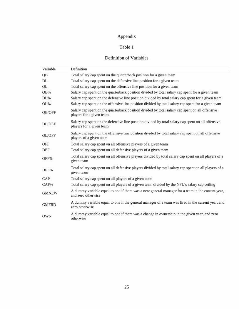
Table 1

Definition of Variables

Variable Definition QB Total salary cap spent on the quarterback position for a given team DL Total salary cap spent on the defensive line position for a given team OL Total salary cap spent on the offensive line position for a given team QB% Salary cap spent on the quarterback position divided by total salary cap spent for a given team DL% Salary cap spent on the defensive line position divided by total salary cap spent for a given team OL% Salary cap spent on the offensive line position divided by total salary cap spent for a given team

QB/OFF Salary cap spent on the quarterback position divided by total salary cap spent on all offensive players for a given team

DL/DEF Salary cap spent on the defensive line position divided by total salary cap spent on all offensive players for a given team

OL/OFF Salary cap spent on the offensive line position divided by total salary cap spent on all offensive players of a given team

OFF Total salary cap spent on all offensive players of a given team DEF Total salary cap spent on all defensive players of a given team

OFF% Total salary cap spent on all offensive players divided by total salary cap spent on all players of a given team

DEF% Total salary cap spent on all defensive players divided by total salary cap spent on all players of a given team

CAP Total salary cap spent on all players of a given team CAP% Total salary cap spent on all players of a given team divided by the NFL’s salary cap ceiling

GMNEW A dummy variable equal to one if there was a new general manager for a team in the current year, and zero otherwise

GMFRD A dummy variable equal to one if the general manager of a team was fired in the current year, and zero otherwise

OWN A dummy variable equal to one if there was a change in ownership in the given year, and zero otherwise

25

Table 2

NFL Salary Cap by Year

Year Salary Cap

2006 $102 million

2007 $109 million

2008 $116 million

2009 $123 million

2010 Uncapped*

2011 $120.6 million

2012 $123 million

2013 $133 million

* No salary cap during the 2010 season

26

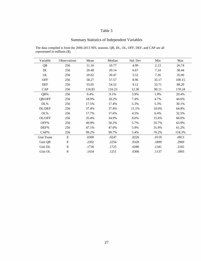
Table 3

Summary Statistics of Independent Variables The data compiled is from the 2006-2013 NFL seasons. QB, DL, OL, OFF, DEF, and CAP are all represented in millions ($).

Variable Observations Mean Median Std. Dev Min Max

QB 256 11.16 10.77 4.99 2.13 26.74 DL 256 20.48 20.14 6.67 7.24 38.44 OL 256 20.62 20.47 5.52 7.26 35.00

OFF 256 58.27 57.57 8.96 35.17 100.15 DEF 256 55.05 54.52 9.12 33.71 88.20 CAP 256 116.83 116.23 12.36 90.11 178.24 QB% 256 9.4% 9.1% 3.9% 1.9% 20.4%

QB/OFF 256 18.9% 18.2% 7.4% 4.7% 44.6% DL% 256 17.5% 17.4% 5.3% 5.3% 30.1%

DL/DEF 256 37.4% 37.4% 11.1% 10.0% 64.8% OL% 256 17.7% 17.6% 4.5% 6.4% 32.5%

OL/OFF 256 35.4% 34.9% 8.0% 15.6% 60.0% OFF% 256 49.9% 50.2% 5.7% 35.7% 63.9% DEF% 256 47.1% 47.0% 5.9% 31.9% 61.2% CAP% 256 99.2% 99.7% 5.4% 76.2% 118.3%

Gini Team 8 .0309 .0247 .0226 .0119 .0813 Gini QB 8 .2302 .2256 .0328 .1899 .2969 Gini DL 8 .1736 .1725 .0280 .1341 .2165 Gini OL 8 .1434 .1251 .0306 .1137 .1893

27

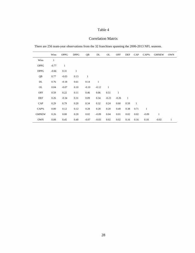
Table 4

Correlation Matrix

There are 256 team-year observations from the 32 franchises spanning the 2006-2013 NFL seasons.

Wins OPPG DPPG QB DL OL OFF DEF CAP CAP% GMNEW OWN

Wins 1

OPPG -0.77 1

DPPG -0.66 0.31 1

QB 0.77 -0.03 0.13 1

DL 0.76 -0.18 0.61 0.14 1

OL 0.04 -0.07 0.10 -0.10 -0.12 1

OFF 0.59 0.22 0.11 0.46 0.06 0.51 1

DEF 0.26 -0.34 0.31 0.09 0.34 -0.23 -0.26 1

CAP 0.29 0.79 0.20 0.34 0.32 0.24 0.60 0.59 1

CAP% 0.00 0.12 0.12 0.28 0.28 0.20 0.49 0.38 0.71 1

GMNEW 0.26 0.00 0.20 0.02 -0.09 0.04 0.01 0.02 0.02 -0.09 1

OWN 0.08 0.45 0.40 -0.07 -0.03 0.02 0.02 0.16 0.16 0.18 -0.02 1

28

Table 5

Determinants of Team Wins

This table contains results from an OLS regression clustered by each individual NFL franchise. The dependent variable is number of wins a team earns in the regular season. There are 256 team-year observations from the 32 franchises spanning the 2006-2013 NFL seasons. The coefficient estimates are listed with associated p-values. *, **, and *** note significance at the 10%, 5%, and 1% levels.

R2 = 0.20

The dependent variable, number of wins in the regular season, is significantly correlated with both the total cap space spent on offensive linemen and the percentage of the NFL salary cap a team spends in a season.

Variable Coefficient P-Value

QB -0.08612 0.771

DL -0.0688 0.761

OL -0.6384** 0.037

QB/OFF 7.7972 0.646

DL/DEF 0.1286 0.993

OL/OFF 34.2022 0.102

OFF -0.3590 0.585

OFF% 75.8071 0.255

DEF -0.9091 0.260

DEF% 114.9002 0.174

CAP 0.7410 0.289

CAP% 12.3023*** 0.002

GMNEW -0.6453 0.262

GMFRD -2.5767 0.000

OWN -1.8362 0.080

29

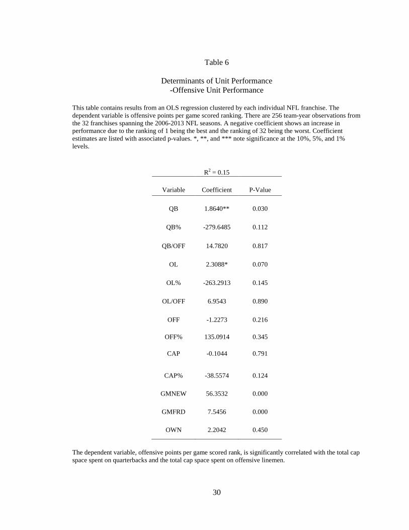
Table 6

Determinants of Unit Performance -Offensive Unit Performance

This table contains results from an OLS regression clustered by each individual NFL franchise. The dependent variable is offensive points per game scored ranking. There are 256 team-year observations from the 32 franchises spanning the 2006-2013 NFL seasons. A negative coefficient shows an increase in performance due to the ranking of 1 being the best and the ranking of 32 being the worst. Coefficient estimates are listed with associated p-values. *, **, and *** note significance at the 10%, 5%, and 1% levels.

R2 = 0.15

Variable

Coefficient

P-Value

QB

1.8640**

0.030

QB%

-279.6485

0.112

QB/OFF

14.7820

0.817

OL

2.3088*

0.070

OL%

-263.2913

0.145

OL/OFF

6.9543

0.890

OFF

-1.2273

0.216

OFF%

135.0914

0.345

CAP

-0.1044

0.791

CAP% -38.5574 0.124

GMNEW 56.3532 0.000

GMFRD 7.5456 0.000

OWN 2.2042 0.450

The dependent variable, offensive points per game scored rank, is significantly correlated with the total cap space spent on quarterbacks and the total cap space spent on offensive linemen.

30

Table 7

Determinants of Unit Performance -Defensive Unit Performance

This table contains results from an OLS regression clustered by each individual NFL franchise. The dependent variable is defensive points per game allowed ranking. There are 256 team-year observations from the 32 franchises spanning the 2006-2013 NFL seasons. A negative coefficient shows an increase in performance due to the ranking of 1 being the best and the ranking of 32 being the worst. Coefficient estimates are listed with associated p-values. *, **, and *** note significance at the 10%, 5%, and 1% levels.

R2 = 0.12

Variable

Coefficient

P-Value

DL

0.4784

0.606

DL%

15.8281

0.905

DL/DEF -27.1620 0.489

DEF

0.9396

0.305

DEF%

-158.9495

0.170

CAP

-0.5239

0.197

CAP%

-22.84771

0.115

GMNEW

1.9385

0.201

GMFRD

6.0873

0.000

OWN

2.6905

0.399

There are no significant relationships between the dependent variable, defensive points allowed per game rank, and any of the independent variables.

31

Table 8

Gini Coefficients of Total Salary Cap Spent Amongst NFL Teams The 2006-2009 seasons fall under the rules of the 1993 CBA. The 2010 season is an uncapped year where there are no limits on salary cap spending. The 2011-2013 seasons are played under the rules of the 2011 CBA.

*shaded region indicates the uncapped 2010 season

There is a significant rise in team Gini coefficients after the implementation of the 2011 CBA.

Year

Gini

2006

0.016

2007

0.012

2008

0.016

2009

0.020

2010

0.081

2011

0.042

2012

0.030

2013

0.029

32

Figure 1

Comparison of Mean Gini Coefficients by Team Adhering to Different CBAs

*2010 season omitted due to lack of salary cap

0

0.005

0.01

0.015

0.02

0.025

0.03

0.035

0.04

Team Gini

Mean Gini by Team, 2006-2013, omitting 2010 season

2006-2009 (1993 CBA)

2011-2013 (2011 CBA)

33

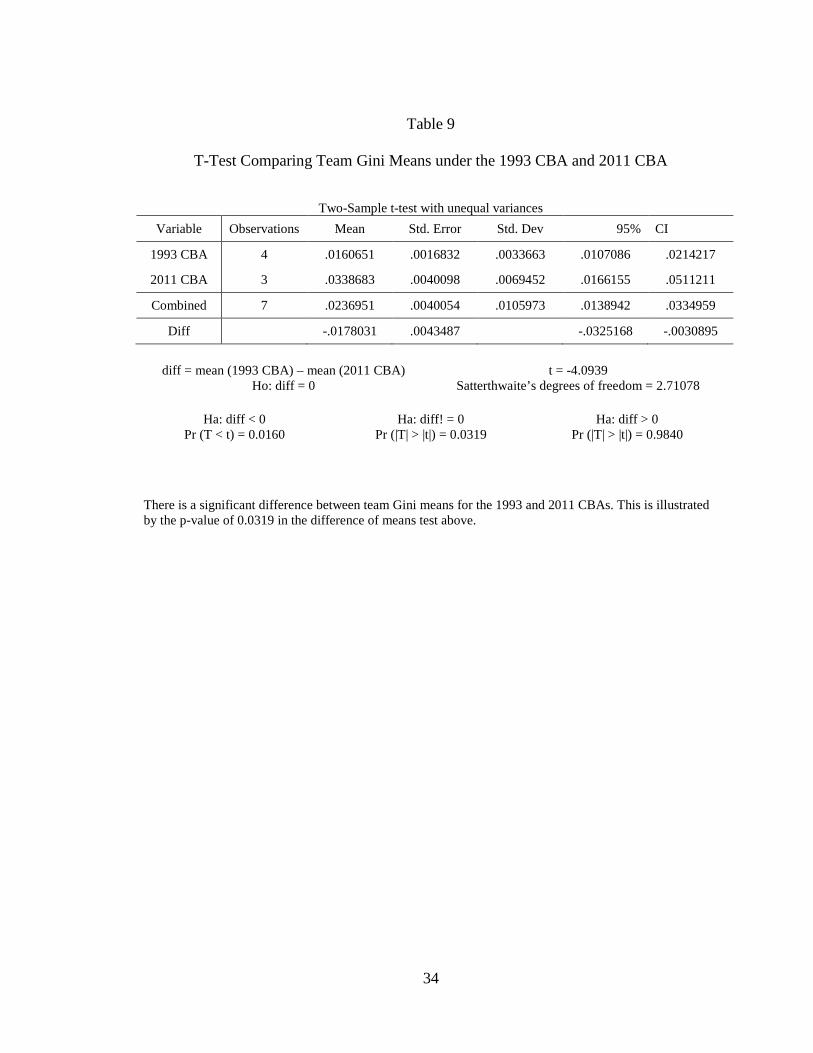
Table 9

T-Test Comparing Team Gini Means under the 1993 CBA and 2011 CBA

Two-Sample t-test with unequal variances Variable Observations Mean Std. Error Std. Dev 95% CI

1993 CBA 4 .0160651 .0016832 .0033663 .0107086 .0214217

2011 CBA 3 .0338683 .0040098 .0069452 .0166155 .0511211

Combined 7 .0236951 .0040054 .0105973 .0138942 .0334959

Diff -.0178031 .0043487 -.0325168 -.0030895

diff = mean (1993 CBA) – mean (2011 CBA) t = -4.0939

Ho: diff = 0 Satterthwaite’s degrees of freedom = 2.71078

Ha: diff < 0 Ha: diff! = 0 Ha: diff > 0 Pr (T < t) = 0.0160 Pr (|T| > |t|) = 0.0319 Pr (|T| > |t|) = 0.9840

There is a significant difference between team Gini means for the 1993 and 2011 CBAs. This is illustrated by the p-value of 0.0319 in the difference of means test above.

34

Table 10

Inter-Team Gini Coefficients by Position

The 2006-2009 seasons fall under the rules of the 1993 CBA. The 2010 season is an uncapped year where there are no limits on salary cap spending. The 2011-2013 seasons are played under the rules of the 2011 CBA. *shaded region indicates the uncapped 2010 season There is a significant increase in all positional Gini coefficients after the implementation of the 2011 CBA.

Year

Gini QB

Gini DL

Gini OL

2006

0.205

0.171

0.127

2007

0.213

0.160

0.114

2008

0.217

0.142

0.122

2009

0.190

0.134

0.123

2010

0.235

0.174

0.171

2011

0.297

0.196

0.189

2012

0.236

0.195

0.179

2013

0.248

0.217

0.122

35

Figure 2

Comparison of Mean Gini Coefficients by Position Adhering to Different CBAs

*2010 season omitted due to lack of salary cap

0

0.05

0.1

0.15

0.2

0.25

0.3

Gini QB Gini DL Gini OL

Mean Gini by Position, 2006-2013, omitting 2010 season

2006-2009 (1993 CBA)

2011-2013 (2011 CBA)

36

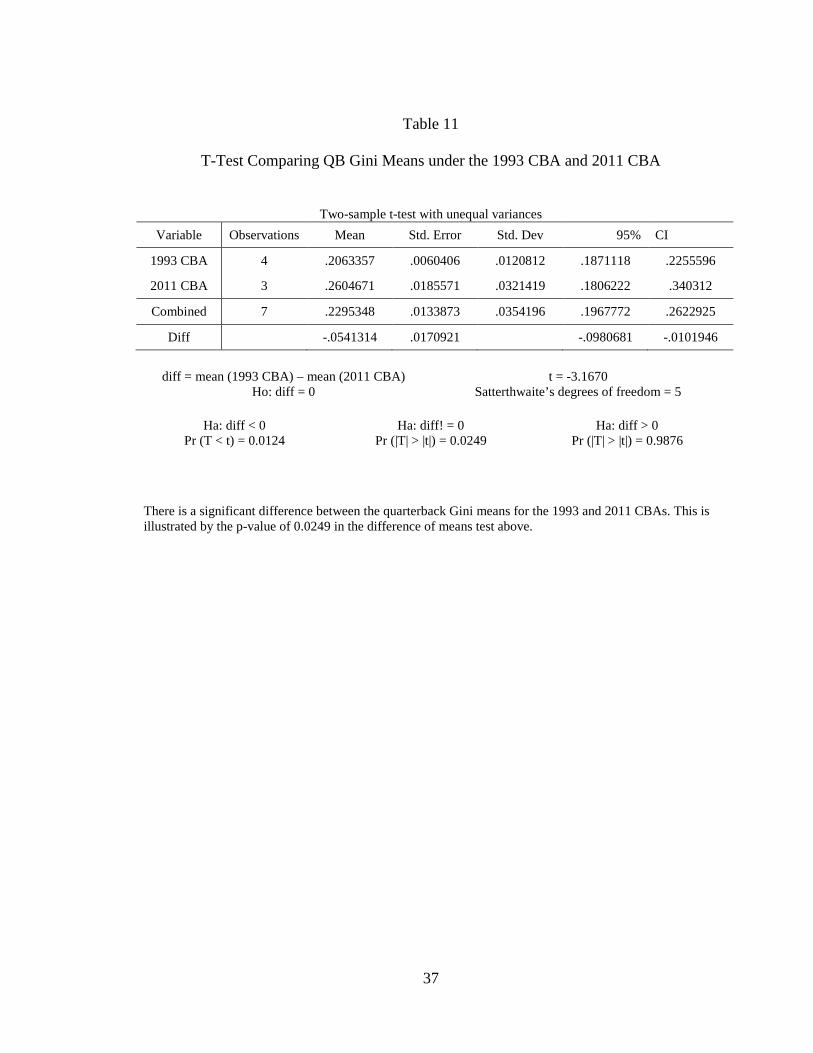
Table 11

T-Test Comparing QB Gini Means under the 1993 CBA and 2011 CBA

Two-sample t-test with unequal variances Variable Observations Mean Std. Error Std. Dev 95% CI

1993 CBA 4 .2063357 .0060406 .0120812 .1871118 .2255596

2011 CBA 3 .2604671 .0185571 .0321419 .1806222 .340312

Combined 7 .2295348 .0133873 .0354196 .1967772 .2622925

Diff -.0541314 .0170921 -.0980681 -.0101946

diff = mean (1993 CBA) – mean (2011 CBA) t = -3.1670

Ho: diff = 0 Satterthwaite’s degrees of freedom = 5

Ha: diff < 0 Ha: diff! = 0 Ha: diff > 0 Pr (T < t) = 0.0124 Pr (|T| > |t|) = 0.0249 Pr (|T| > |t|) = 0.9876

There is a significant difference between the quarterback Gini means for the 1993 and 2011 CBAs. This is illustrated by the p-value of 0.0249 in the difference of means test above.

37

Table 12

T-Test Comparing Defensive Linemen Gini Means under the 1993 CBA and 2011 CBA.

Two-sample t-test with unequal variances

Variable Observations Mean Std. Error Std. Dev 95% CI

1993 CBA 4 .1519129 .0083315 .016663 .1253984 .1784275

2011 CBA 3 .2022582 .0071355 .0123591 .1715565 .2329599

Combined 7 .1734895 .0114263 .0302312 .1455302 .2014487

Diff -.0503453 .0115248 -.0799707 -.0207199

diff = mean (1993 CBA) – mean (2011 CBA) t = -4.3684

Ho: diff = 0 Satterthwaite’s degrees of freedom = 5

Ha: diff < 0 Ha: diff! = 0 Ha: diff > 0 Pr (T < t) = 0.0036 Pr (|T| > |t|) = 0.0072 Pr (|T| > |t|) = 0.9964

There is a significant difference between the defensive line Gini means for the 1993 and 2011 CBAs. This is illustrated by the p-value of 0.0072 in the difference of means test above.

38

Table 13

T-Test Comparing Offensive Linemen Gini Means for 1993 CBA and 2011 CBA

Two-sample t-test with unequal variances

Variable Observations Mean Std. Error Std. Dev 95% CI

1993 CBA 4 .1215867 .0028643 .0057285 .1124713 .1307021

2011 CBA 3 .1633489 .0208761 .0361585 .0735262 .2531715

Combined 7 .1394848 .0116529 .0308306 .1109712 .1679984

Diff -.0417622 .017792 -.0874979 .0039735

diff = mean (1993 CBA) – mean (2011 CBA) t = -2.3473

Ho: diff = 0 Satterthwaite’s degrees of freedom = 5

Ha: diff < 0 Ha: diff! = 0 Ha: diff > 0 Pr (T < t) = 0.0329 Pr (|T| > |t|) = 0.0658 Pr (|T| > |t|) = 0.9671

There is a significant difference between the offensive line Gini means for the 1993 and 2011 CBAs. This is illustrated by the p-value of 0.0658 in the difference of means test above.

39

Works Cited "Big Bath Definition | Investopedia." Investopedia. N.p., n.d. Web. 1 Nov. 2014. Borghesi, Richard. "Allocation of scarce resources: Insight from the NFL salary cap." Journal of Economics and Business 60.6 (2008): 536-550. "Contract Status of 2010 First-round Draft Picks." NFL.com. N.p., 6 July 2010. Web. 28 Oct. 2014. Gaines, Cork. "The 25 Highest-Paid Players In The NFL." Business Insider. Business Insider, Inc, 3 Sept. 2014. Web. 5 Nov. 2014. Kirk, Jason. "All 15 NFL 3-4 Defenses Ranked by Weight (plus Falcons Takeaways).”

The Falcoholic. SB Nation, 17 Mar. 2014. Web. 1 Nov. 2014.

Kowalewski, Sandra, and Michael A. Leeds. “The Impact of the Salary Cap and Free Agency on the Structure and Distribution of Salaries in the NFL.” Sports Economics: Current Research. Praeger, Westport, CT (1999). Larsen, Andrew, Aju J. Fenn, and Erin Leanne Spenner. “The impact of free agency and the salary cap on competitive balance in the National Football League.” Journal of Sports Economics 7.4 (2006): 374-390 Lazear, Edward P. “Pay equality and industrial politics.” Journal of Political Economy (1989): 561-580. Lazear, Edward P. “Labor economics and the psychology of organizations.” The Journal Of Economic Perspectives (1991): 89-110. Leeds, Michael A., and Sandra Kowalewski. “Winner Take All in the NFL: The Effect of the Salary Cap and Free Agency on the Compensation of Skill Position Players.” Journal of Sports Economics 2.3 (2001): 244-256 Quinn, Kevin G., Melissa Geier, and Anne Berkovitz. Superstars and Journeymen: An Analysis of National Football Team’s Allocation of the Salary Cap across Rosters, 2000-2005. No. 0722. 2007 Rosen, Sherwin. “The economics of superstars.” The American Economic Review (1981): 845-858. Rosenthal, Gregg. “Cowboys, Redskins Lead the Way in Uncapped Spending” ProFootballTalk. N.p., 18 Sept. 2010. Web. 1 Nov. 2014

40

Endnotes

1 There are a few exceptions where teams can go above the salary cap limit. An example of this includes a team’s salary cap carry over where they are allowed to carry over unused salary cap space into future years. 2 Players in the 25th quantile are comprised of the players in the income distribution quantile from .2-.3. Players in the 75th quantile are comprised of players in the income distribution quantile from .6-.8. 3 Gini coefficients are calculated by finding the area between the Lorenz curve and the line of perfect equality and dividing it by 0.5. 4 The NFL draft consists of seven rounds and the order of each round is determined in reverse order of its record the previous year. Therefore, the last place team in the NFL picks first and so on. 5 As noted by the Business Insider list of the highest-paid players in the NFL 6 There are currently 15 teams starting three defensive linemen while the other 17 teams start four. 7 The big bath is a financial statement manipulation strategy where upper management concludes they will not meet earning targets so they manipulate the financials to take as big of a loss as possible. The rationale behind this is to artificially increase earnings in future years to paint management in a better light. 8 For example, the Dallas Cowboys signed Miles Austin to a contract with a $17 million base salary in the year 2010. 9 The top-five picks of the 2010 NFL draft all received contracts north of $60 million with every contract containing at least $30 million of guaranteed money. Sam Bradford, the first pick of the 2010 draft, became the second-highest player in the NFL in 2011 before ever taking at the NFL level.

41