place & route tutorial #1 - ncsu eda wiki · place & route tutorial #1 in this tutorial you...

NC State University Fall 2016 ECE Department ECE 720 W. Rhett Davis

Place & Route Tutorial #1

In this tutorial you will use Synopsys IC Compiler (ICC) to place, route, and analyze the timing and wire-length of two simple designs. This tutorial assumes that you have worked through Tutorial #1: Introduction to Simulation and Synthesis on the ECE 520 ASIC Design Tutorials Page and that you know how to simulate, synthesize and analyze timing on basic designs.

I. Setup

Log in to a Linux machine.

Download and unpack the file pr_tut1.tar.gz. This archive contains a directory called ''pr_tut1'' with two subdirectories called “counter” and “xbar”. Each of these directories contains two subdirectories called ''v'' and ''pr'' with files needed to complete this tutorial. We will start with the counter design and move on to the xbar design.

Change to the counter/v/synth directory and synthesize the simple ''counter.v'' design with the command “make”. This design is copied from the ECE 520 tutorial #1 mentioned above. When complete, you should have a file called “counter/v/src/gate/counter_final.v”, which will serve as the starting point for this tutorial.

II. Initialize the Design

1. Change to the PR directory and Start ICC with the command “make gui”. Look inside the Makefile, and you’ll see that this recipe executes the following commands

2. Once the ICC Main Window appears, type the command “source import.tcl” at the icc_shell>

prompt at the bottom of the window. You may want to open the import.tcl file in a separate window to see what’s inside. If you do, you’ll notice that it’s doing the following: (You should update these details as needed to for your own designs)

Sources setup.tcl – The setup.tcl file defines various variables used throughout the design flow. In particular, it sets a variable used in the remainder of the file called modname, which is the module-name, set to “counter” for this tutorial. This file gives the standard-cell netlist that will be placed and routed.

Creates the MilkyWay library – The next command creates a library called “work” in the current directory to store all results. This library is in the Synopsys MilkyWay database format and uses a 32nm technology file and standard-cell library.

Imports the Verilog Netlist – The Verilog netlist is imported into a cell called “counter_init” (i.e. initialized). To successfully import the file, the path is specified, along with the name of the top-level cell in the Verilog file.

Sources the Timing Constraint File - This reads the timing constraint(s) that will be used for the design. The file loaded is almost identical to the “Constrainsts.tcl” file used earlier to synthesize the design with Synopsys Design Compiler. Look in this file and you'll see that it defines the clock port and a 10 ns clock period.

add synopsys2015 icc_shell -gui


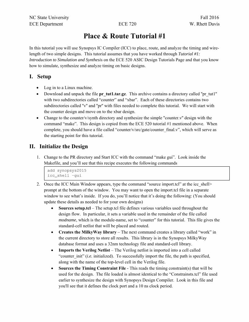
3. At this point, your design should look like the figure below. To make your view look exactly like the one below, you will need to edit the “View Settings”. You can do that by using F8 or by selecting View → Toolbars → View Settings. Then select the check-boxes in the “Vis.” column (i.e. “visible”) for object types Pin and Site Row and then click the “Apply” button. You can

zoom in by left-clicking on the zoom-tool and draging a box. Some convenient key-bindings are included below.

4. Now that the design has been loaded, you can analyze the timing of the design. Type the command “report_timing” in the Main Window icc_shell> prompt. This timing report should look identical to the report in Design Compiler. The slack on the critical path is 7.7901 ns. This is pretty good! Our clock period is not set very aggressively for this design. If we reduce the clock period in the constraints.tcl file by more than 7.7901ns, then we will see a negative number here. Compare this to the critical path given in the file ''../v/synth/timing_max_slow_holdfixed_tut1.rpt'', and you'll note that the path and delay are

Button/Key Action Description

Select Tool Allows selection of objects in the Layout Window q Query

Selection Display the object attributes for the selected object.

f Fit Display Zooms the display to fit the design area.

z Zoom Tool Selects the Zoom tool

+ Zoom-in Zooms in the display, 2x.

Shift-z or - Zoom-out Zooms out the display, 2x.

Arrows Pan Pans the display in direction of arrow.

Ctrl-U Ruler Selects the Ruler tool for measuring distance.

Clear Rulers Clears all rulers in the view.


identical. This is no great surprise, since ICC and Design Compiler are using the same timing engine.

5. Lastly, note that all of the output that you see in the Main Window is also appearing in the UNIX shell window where you typed “make gui”. This output is also recorded in the file icc_output.log. We’ll be referring to this file throughout the rest of this tutorial.

III. Place & Route the Design

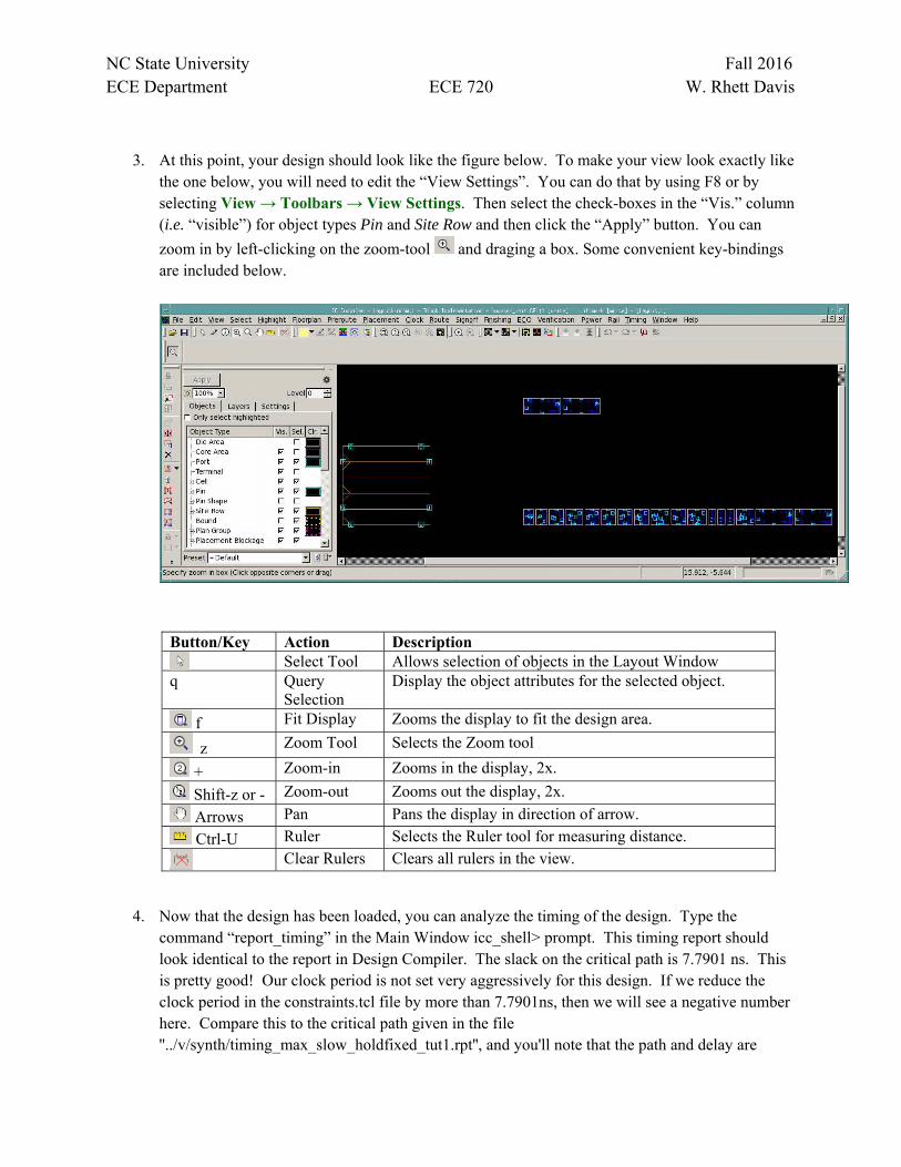
Choose Placement → Core Placement and Optimization… to run the Placer. Click OK on the next pop-up to run placement with default options. Once complete, your design should look like the one below.

Choose File → Save Design.... In the Save Design dialog box, check the “Show Advanced Options” box and then scroll to the right until you see the “Save As Name” box. Enter the name “counter_placed” and check the “Save As” box to the left of the name. Then click Ok. Once saved, you can open the design with File → Open Design... in the ICC Main Window.

Choose Route → Global Route… and click OK on the next pop-up to route with default options. Your routed design should look like the one below. The only difference you should see will be that some vias have been added to connect from one metal layer to another, but no wires have been routed, yet. This is because the Global Route performs only the first part of the routing process. That is, all wires are assigned to Global Routing Cells (GRCs).


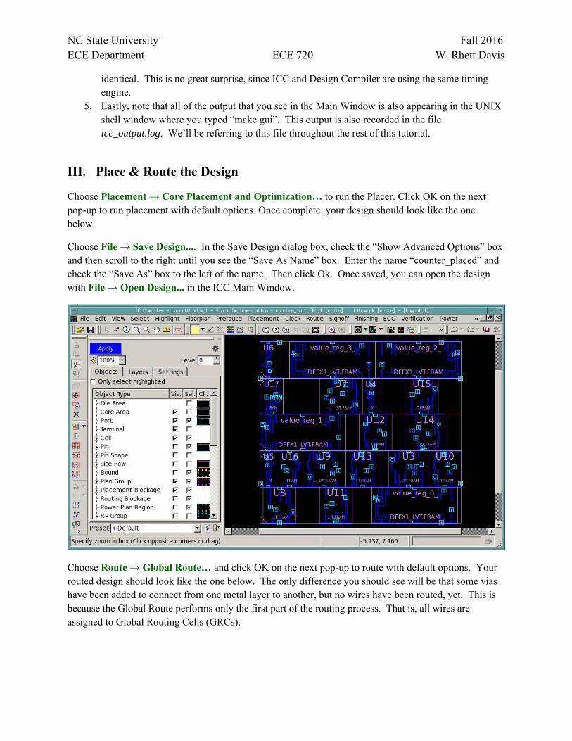
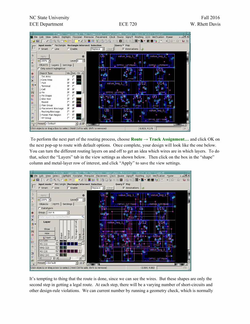
To perform the next part of the routing process, choose Route → Track Assignment… and click OK on the next pop-up to route with default options. Once complete, your design will look like the one below. You can turn the different routing layers on and off to get an idea which wires are in which layers. To do that, select the “Layers” tab in the view settings as shown below. Then click on the box in the “shape” column and metal-layer row of interest, and click “Apply” to save the view settings.

It’s tempting to thing that the route is done, since we can see the wires. But these shapes are only the second step in getting a legal route. At each step, there will be a varying number of short-circuits and other design-rule violations. We can current number by running a geometry check, which is normally


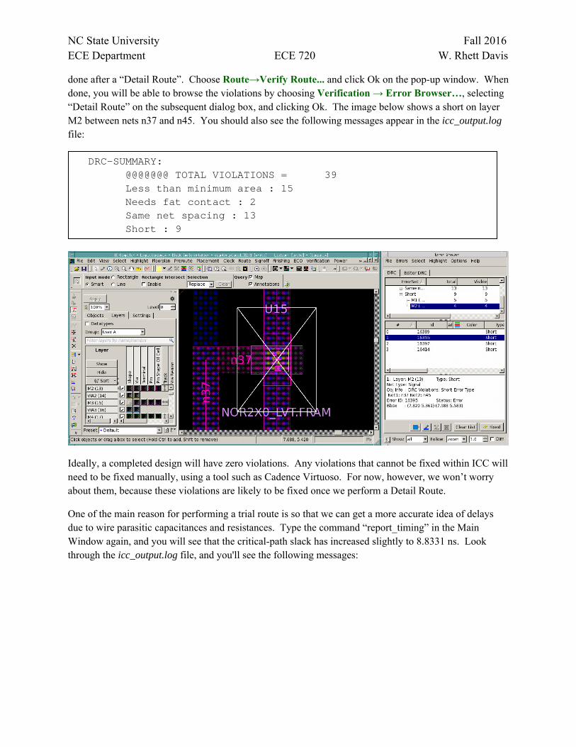
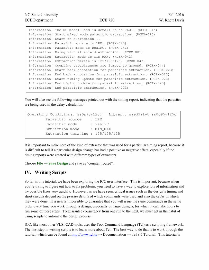
done after a “Detail Route”. Choose Route→Verify Route... and click Ok on the pop-up window. When done, you will be able to browse the violations by choosing Verification → Error Browser…, selecting “Detail Route” on the subsequent dialog box, and clicking Ok. The image below shows a short on layer M2 between nets n37 and n45. You should also see the following messages appear in the icc_output.log file:

Ideally, a completed design will have zero violations. Any violations that cannot be fixed within ICC will need to be fixed manually, using a tool such as Cadence Virtuoso. For now, however, we won’t worry about them, because these violations are likely to be fixed once we perform a Detail Route.

One of the main reason for performing a trial route is so that we can get a more accurate idea of delays due to wire parasitic capacitances and resistances. Type the command “report_timing” in the Main Window again, and you will see that the critical-path slack has increased slightly to 8.8331 ns. Look through the icc_output.log file, and you'll see the following messages:

DRC-SUMMARY: @@@@@@@ TOTAL VIOLATIONS = 39 Less than minimum area : 15 Needs fat contact : 2 Same net spacing : 13 Short : 9


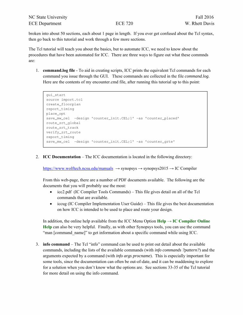
You will also see the following messages printed out with the timing report, indicating that the parasitcs are being used in the delay calculation:

It is important to make note of the kind of extractor that was used for a particular timing report, because it is difficult to tell if a particular design change has had a positive or negative effect, especially if the timing reports were created with different types of extractors.

Choose File → Save Design and save as "counter_routed".

IV. Writing Scripts

So far in this tutorial, we have been exploring the ICC user interface. This is important, because when you’re trying to figure out how to fix problems, you need to have a way to explore lots of information and try possible fixes very quickly. However, as we have seen, critical issues such as the design’s timing and short circuits depend on the precise details of which commands were used and also the order in which they were done. It is nearly impossible to guarantee that you will issue the same commands in the same order every time you work through a design, especially on large designs, for which it can take hours to run some of these steps. To guarantee consistency from one run to the next, we must get in the habit of using scripts to automate the design process.

ICC, like most other VLSI CAD tools, uses the Tool Command Language (Tcl) as a scripting framework. The first step in writing scripts is to learn more about Tcl. The best way to do that is to work through the tutorial, which can be found at http://www.tcl.tk → Documentation → Tcl 8.5 Tutorial. This tutorial is

Operating Conditions: ss0p95v125c Library: saed32lvt_ss0p95v125c Parasitic source : LPE Parasitic mode : RealRC Extraction mode : MIN_MAX Extraction derating : 125/125/125

Information: The RC model used is detail route TLU+. (RCEX-015) Information: Start mixed mode parasitic extraction. (RCEX-023) Information: Start rc extraction... Information: Parasitic source is LPE. (RCEX-040) Information: Parasitic mode is RealRC. (RCEX-041) Information: Using virtual shield extraction. (RCEX-081) Information: Extraction mode is MIN_MAX. (RCEX-042) Information: Extraction derate is 125/125/125. (RCEX-043) Information: Coupling capacitances are lumped to ground. (RCEX-044) Information: Start back annotation for parasitic extraction. (RCEX-023) Information: End back annotation for parasitic extraction. (RCEX-023) Information: Start timing update for parasitic extraction. (RCEX-023) Information: End timing update for parasitic extraction. (RCEX-023) Information: End parasitic extraction. (RCEX-023)


broken into about 50 sections, each about 1 page in length. If you ever get confused about the Tcl syntax, then go back to this tutorial and work through a few more sections.

The Tcl tutorial will teach you about the basics, but to automate ICC, we need to know about the procedures that have been automated for ICC. There are three ways to figure out what these commnds are:

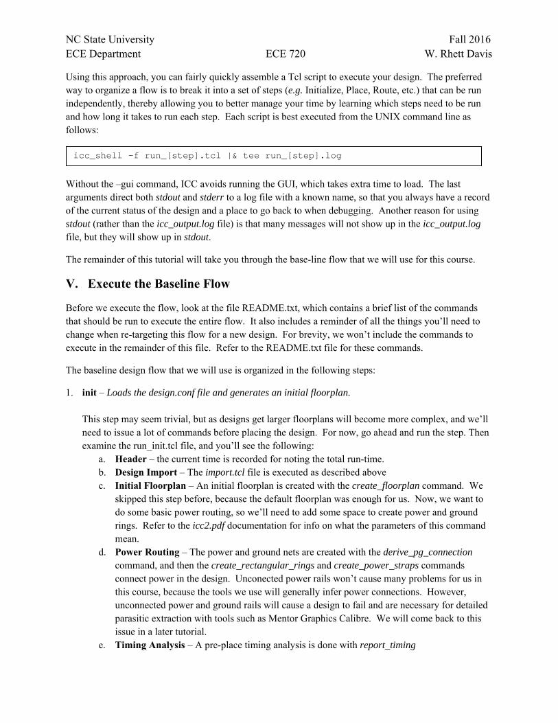
1. command.log file - To aid in creating scripts, ICC prints the equivalent Tcl commands for each command you issue through the GUI. These commands are collected in the file command.log. Here are the contents of my encounter.cmd file, after running this tutorial up to this point:

2. ICC Documentation – The ICC documentation is located in the following directory: https://www.wolftech.ncsu.edu/manuals → synopsys → synopsys2015 → IC Compiler From this web-page, there are a number of PDF documents available. The following are the documents that you will probably use the most:

icc2.pdf (IC Compiler Tools Commands) – This file gives detail on all of the Tcl commands that are available.

iccug (IC Compiler Implementation User Guide) – This file gives the best documentation on how ICC is intended to be used to place and route your design.

In addition, the online help available from the ICC Menu Option Help → IC Compiler Online Help can also be very helpful. Finally, as with other Synopsys tools, you can use the command “man [command_name]” to get information about a specific command while using ICC.

3. info command – The Tcl “info” command can be used to print out detail about the available commands, including the lists of the available commands (with info commands ?pattern?) and the arguments expected by a command (with info args procname). This is especially important for some tools, since the documentation can often be out-of-date, and it can be maddening to explore for a solution when you don’t know what the options are. See sections 33-35 of the Tcl tutorial for more detail on using the info command.

gui_start source import.tcl create_floorplan report_timing place_opt save_mw_cel -design "counter_init.CEL;1" -as "counter_placed" route_zrt_global route_zrt_track verify_zrt_route report_timing save_mw_cel -design "counter_init.CEL;1" -as "counter_grte"


Using this approach, you can fairly quickly assemble a Tcl script to execute your design. The preferred way to organize a flow is to break it into a set of steps (e.g. Initialize, Place, Route, etc.) that can be run independently, thereby allowing you to better manage your time by learning which steps need to be run and how long it takes to run each step. Each script is best executed from the UNIX command line as follows:

Without the –gui command, ICC avoids running the GUI, which takes extra time to load. The last arguments direct both stdout and stderr to a log file with a known name, so that you always have a record of the current status of the design and a place to go back to when debugging. Another reason for using stdout (rather than the icc_output.log file) is that many messages will not show up in the icc_output.log file, but they will show up in stdout.

The remainder of this tutorial will take you through the base-line flow that we will use for this course.

V. Execute the Baseline Flow

Before we execute the flow, look at the file README.txt, which contains a brief list of the commands that should be run to execute the entire flow. It also includes a reminder of all the things you’ll need to change when re-targeting this flow for a new design. For brevity, we won’t include the commands to execute in the remainder of this file. Refer to the README.txt file for these commands.

The baseline design flow that we will use is organized in the following steps:

1. init – Loads the design.conf file and generates an initial floorplan. This step may seem trivial, but as designs get larger floorplans will become more complex, and we’ll need to issue a lot of commands before placing the design. For now, go ahead and run the step. Then examine the run_init.tcl file, and you’ll see the following:

a. Header – the current time is recorded for noting the total run-time. b. Design Import – The import.tcl file is executed as described above c. Initial Floorplan – An initial floorplan is created with the create_floorplan command. We

skipped this step before, because the default floorplan was enough for us. Now, we want to do some basic power routing, so we’ll need to add some space to create power and ground rings. Refer to the icc2.pdf documentation for info on what the parameters of this command mean.

d. Power Routing – The power and ground nets are created with the derive_pg_connection command, and then the create_rectangular_rings and create_power_straps commands connect power in the design. Unconected power rails won’t cause many problems for us in this course, because the tools we use will generally infer power connections. However, unconnected power and ground rails will cause a design to fail and are necessary for detailed parasitic extraction with tools such as Mentor Graphics Calibre. We will come back to this issue in a later tutorial.

e. Timing Analysis – A pre-place timing analysis is done with report_timing

icc_shell -f run_[step].tcl |& tee run_[step].log


f. Save Design – The design is saved, so that we can start from this point on the next step. We can also start up ICC and open this design to view its status after this step.

g. Footer – The elapsed time is printed, along with a message that the command completed successfully. This message is important, because when running a lot of scripts, it can be hard to find where things went wrong sometimes. The first thing that we should always check is whether or not a script completed successfully, or whether the script failed for some reason during execution.

2. place – Places the standard cells This command is much like the previous step, except that it opens the counter_init design, places the cells (as we did interactively earlier) with the place_opt command, and then saves the design as counter_placed. Go ahead and run this step now.

3. cts – Clock-Tree Synthesis This command is like the previous step, but runs clock-tree synthesis with the clock_opt command. We skipped this step earlier for simplicity. We will come back to clock-tree synthesis in a later tutorial, but it is such an important part of the flow that it’s best not to skip completely. Go ahead and run this step now. We will discuss clock-trees in more detail in a future tutorial.

4. route – Global and Detail route, extraction, and timing analysis This step executes the following sub-steps:

a. Set Routing Options & Constraints – The most important constraint for this tutorial is the number of metal layers to use, which is set with the set_net_routing_layer_constraints –max_layer_name option. Here it is set to M9, the maximum, but it is better to route with fewer metal layers to save money in manufacturing.

b. Global Route – The global route is executed with the command route_opt –stage global. The detail route step that follows would perform a global route automatically, so it’s not necessary to issue this command explicitly. We listed the global route separately here in case you want to perform a quick check for routing congestion, since the detail route can take a very, very long time, if the design is very congested.

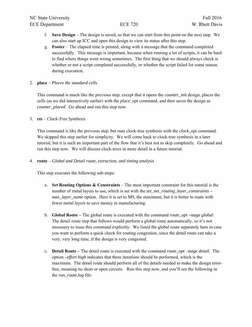
c. Detail Route – The detail route is executed with the command route_opt –stage detail. The option –effort high indicates that three iterations should be performed, which is the maximum. The detail route should perform all of the details needed to make the design error-free, meaning no short or open circuits. Run this step now, and you’ll see the following in the run_route.log file:


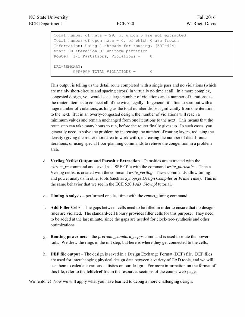
This output is telling us the detail route completed with a single pass and no violations (which are mainly short-circuits and spacing errors) in virtually no time at all. In a more complex, congested design, you would see a large number of violations and a number of iterations, as the router attempts to connect all of the wires legally. In general, it’s fine to start out with a huge number of violations, as long as the total number drops significantly from one iteration to the next. But in an overly-congested design, the number of violations will reach a minimum values and remain unchanged from one iterations to the next. This means that the route step can take many hours to run, before the router finally gives up. In such cases, you generally need to solve the problem by increasing the number of routing layers, reducing the density (giving the router more area to work with), increasing the number of detail-route iterations, or using special floor-planning commands to relieve the congention in a problem area.

d. Verilog Netlist Output and Parasitic Extraction – Parasitics are extracted with the extract_rc command and saved as a SPEF file with the command write_parasitics. Then a Verilog netlist is created with the command write_verilog. These commands allow timing and power analysis in other tools (such as Synopsys Design Compiler or Prime Time). This is the same behavior that we see in the ECE 520 PAD_Flow.pl tutorial.

e. Timing Analysis – performed one last time with the report_timing command.

f. Add Filler Cells – The gaps between cells need to be filled in order to ensure that no design-rules are violated. The standard-cell library provides filler cells for this purpose. They need to be added at the last minute, since the gaps are needed for clock-tree-synthesis and other optimizations.

g. Routing power nets – the preroute_standard_cepps command is used to route the power rails. We drew the rings in the init step, but here is where they get connected to the cells.

h. DEF file output – The design is saved in a Design Exchange Format (DEF) file. DEF files are used for interchanging physical design data between a variety of CAD tools, and we will use them to calculate various statistics on our design. For more information on the format of this file, refer to the lefdefref file in the resources sections of the course web-page.

We’re done! Now we will apply what you have learned to debug a more challenging design.

Total number of nets = 29, of which 0 are not extracted Total number of open nets = 0, of which 0 are frozen Information: Using 1 threads for routing. (ZRT-444) Start DR iteration 0: uniform partition Routed 1/1 Partitions, Violations = 0 DRC-SUMMARY: @@@@@@@ TOTAL VIOLATIONS = 0


VI. Place & Route the Crossbar Design

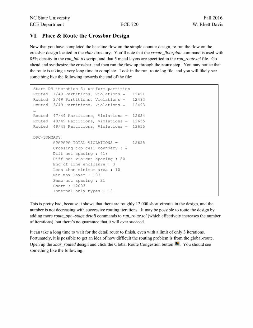
Now that you have completed the baseline flow on the simple counter design, re-run the flow on the crossbar design located in the xbar directory. You’ll note that the create_floorplan command is used with 85% density in the run_init.tcl script, and that 5 metal layers are specified in the run_route.tcl file. Go ahead and synthesize the crossbar, and then run the flow up through the route step. You may notice that the route is taking a very long time to complete. Look in the run_route.log file, and you will likely see something like the following towards the end of the file:

This is pretty bad, because it shows that there are roughly 12,000 short-circuits in the design, and the number is not decreasing with successive routing iterations. It may be possible to route the design by adding more route_opt –stage detail commands to run_route.tcl (which effectively increases the number of iterations), but there’s no guarantee that it will ever succeed.

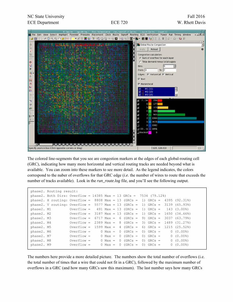
It can take a long time to wait for the detail route to finish, even with a limit of only 3 iterations. Fortunately, it is possible to get an idea of how difficult the routing problem is from the global-route. Open up the xbar_routed design and click the Global Route Congestion button . You should see something like the following:

Start DR iteration 3: uniform partition Routed 1/49 Partitions, Violations = 12491 Routed 2/49 Partitions, Violations = 12493 Routed 3/49 Partitions, Violations = 12493 … Routed 47/49 Partitions, Violations = 12684 Routed 48/49 Partitions, Violations = 12655 Routed 49/49 Partitions, Violations = 12655 DRC-SUMMARY: @@@@@@@ TOTAL VIOLATIONS = 12655 Crossing top-cell boundary : 4 Diff net spacing : 418 Diff net via-cut spacing : 80 End of line enclosure : 3 Less than minimum area : 10 Min-max layer : 103 Same net spacing : 21 Short : 12003 Internal-only types : 13


The colored line-segments that you see are congestion markers at the edges of each global-routing cell (GRC), indicating how many more horizontal and vertical routing tracks are needed beyond what is available. You can zoom into these markers to see more detail. As the legend indicates, the colors correspond to the nuber of overflows for that GRC edge (i.e. the number of wires to route that exceeds the number of tracks available). Look in the run_route.log file, and you’ll see the following output.

The numbers here provide a more detailed picture. The numbers show the total number of overflows (i.e. the total number of times that a wire that could not fit in a GRC), followed by the maximum number of overflows in a GRC (and how many GRCs saw this maximum). The last number says how many GRCs

phase2. Routing result: phase2. Both Dirs: Overflow = 14385 Max = 13 GRCs = 7534 (79.12%) phase2. H routing: Overflow = 8808 Max = 13 (GRCs = 1) GRCs = 4395 (92.31%) phase2. V routing: Overflow = 5577 Max = 13 (GRCs = 1) GRCs = 3139 (65.93%) phase2. M1 Overflow = 491 Max = 13 (GRCs = 1) GRCs = 143 (3.00%) phase2. M2 Overflow = 3187 Max = 13 (GRCs = 1) GRCs = 1650 (34.66%) phase2. M3 Overflow = 6717 Max = 6 (GRCs = 9) GRCs = 3037 (63.79%) phase2. M4 Overflow = 2389 Max = 8 (GRCs = 3) GRCs = 1489 (31.27%) phase2. M5 Overflow = 1599 Max = 4 (GRCs = 6) GRCs = 1215 (25.52%) phase2. M6 Overflow = 0 Max = 0 (GRCs = 0) GRCs = 0 (0.00%) phase2. M7 Overflow = 0 Max = 0 (GRCs = 0) GRCs = 0 (0.00%) phase2. M8 Overflow = 0 Max = 0 (GRCs = 0) GRCs = 0 (0.00%) phase2. M9 Overflow = 0 Max = 0 (GRCs = 0) GRCs = 0 (0.00%)


experience an overflow of at least 1, as an absolute number and as a percentage of the total GRCs. The numbers here show that 79% of all GRCs have overflows, so there’s not a lot of space for those overflowing wires to go. This is a rather congested design, but good Detail Routers can handle a lot of congestion, and the ICC Detail Router is a pretty good one. You can try to add more detail routing iterations, but watch the violations on each iteration in the run_route.log file to make sure that the step doesn’t run forever. Another option is to comment-out the detail routing command and simply run the global-route, checking the congestion information above until you have a good feeling that the detail route will succeed.

Your task is to try to alter the scripts to allow the xbar design to complete the route step successfully with no violations. You can decrease the density of the design, increase the number of metal layers available, and/or increase the number of detail routing iterations. When you are done, turn in the following:

your xbar_routed.def file

your run_route.log file, showing zero violations

all Tcl scripts from your xbar/pr directory

Also include in your solution document a description of the changes that you needed to make to the scripts in order to route the design with no violations.

place & route tutorial #1 - ncsu eda wiki · place & route tutorial #1 in this tutorial you...

Documents