1 out of 15

Analyzing Data: Uncertainty Analysis & Curve Fitting

TABLE OF CONTENTS (ctrl + click section title in table of contents to link directly to section)

1 Accuracy vs. Precision2 Methods for determining uncertainty3 Multiple trials method4 Instrumental uncertainty method5 Propagation of errors: the uncertainty of a computed quantity6 Reporting your results7 Doing your best work in lab8 Tips for taking data: How many points to collect and where to measure them9 Mistakes: What to do when things go wrong10 A final comment

For a more detailed treatment of this topic read Ifan G. Hughes and Thomas P.A. Hase, Measurements and their Uncertainties, Oxford University Press, Oxford, UK (2011)This book is on electronic and permanent hardcopy reserve in the Science Library.

In science, how well you know a value, quantified by the uncertainty of a measured value, is just as important as the measured value itself. You could even say that characterizing errors — the range of uncertainty in a measured value — is one of the distinguishing features of empirical science: only in mathematics do you have exact numbers. This topic is essential to all areas of empirical science (biology, chemistry, epidemiology and public health) not just physics! For this reason, we focus extensively in this course on the essential topic of uncertainty analysis. Note that in this document we will use the words error and uncertainty to mean the same thing; you should not read the word “error” to mean “mistake” or “blunder”.

How do you know you’ve found the Higgs boson? How do you know that a new disease treatment is superior to an older one—or when it’s even harmful? The answers are found in careful experimental measurements and their uncertainties. Let’s see how!

1. Accuracy vs. PrecisionThere are two effects that determine uncertainty: precision (statistical) and accuracy (systematic) uncertainties. No matter how careful you are in making a measurement, there will always be some spread in your data. This introduces an uncertainty called the precision or random error. This spread or “scatter” comes from random variations in variables beyond the experimenter’s control, from variations in how the experimenter takes readings from analog devices (e.g. meter sticks, or meters with needle pointers rather than digital displays), and variations in quantities that are intrinsically random. These random or precision errors have the characteristic of introducing uncertainties in your measured quantity that could both over-estimate and under-estimate with equal probability each time you perform a particular measurement.

2 out of 15

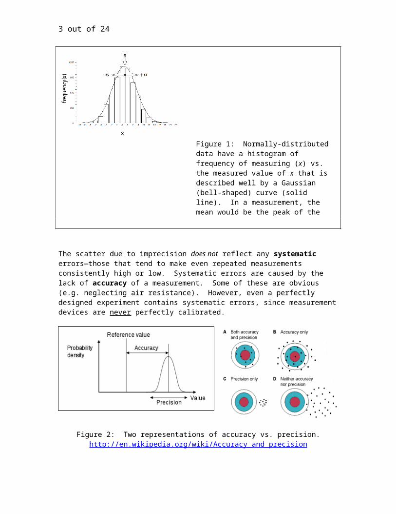
NOTE - Assumptions about statistics: Throughout these notes we will assume that variations in data that occur randomly do so with a consistent distribution of probabilities, and that the variations in different measurements are uncorrelated—that is, they occur independently of each other. These simplifying mathematical assumptions are well-obeyed in many experiments you will perform this semester. In the case of large collections of data (see subsection 3.3 for the case of small samples) the distribution is a Gaussian (bell-shaped curve) (Fig. 1). This is often called the “normal distribution.”

Figure 1: Normally-distributed data have a histogram of frequency of measuring (x) vs. the measured value of x that is described well by a Gaussian (bell-shaped) curve (solid line). In a measurement, the mean would be the peak of the normal distribution and the uncertainties would express how well you knew the position of the mean. (Here the mean is 3.8 and the standard deviation is 4.3)

The scatter due to imprecision does not reflect any systematic errors—those that tend to make even repeated measurements consistently high or low. Systematic errors are caused by the lack of accuracy of a measurement. Some of these are obvious (e.g. neglecting air resistance). However, even a perfectly designed experiment contains systematic errors, since measurement devices are never perfectly calibrated.

3 out of 15

Figure 2: Two representations of accuracy vs. precision. http://en.wikipedia.org/wiki/Accuracy_and_precision

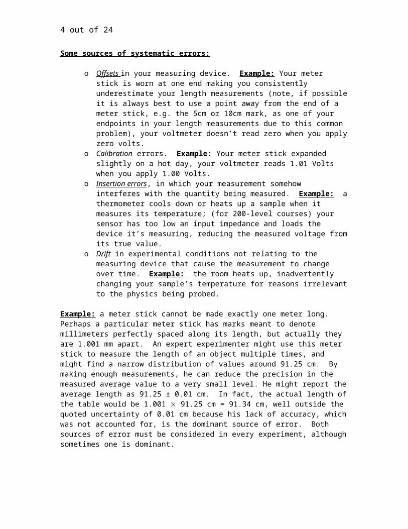
Some sources of systematic errors:

o Offsets in your measuring device. Example: Your meter stick is worn at one end making you consistently underestimate your length measurements (note, if possible it is always best to use a point away from the end of a meter stick, e.g. the 5cm or 10cm mark, as one of your endpoints in your length measurements due to this common problem), your voltmeter doesn’t read zero when you apply zero volts.

o Calibration errors. Example: Your meter stick expanded slightly on a hot day, your voltmeter reads 1.01 Volts when you apply 1.00 Volts.

o Insertion errors , in which your measurement somehow interferes with the quantity being measured. Example: a thermometer cools down or heats up a sample when it measures its temperature; (for 200-level courses) your sensor has too low an input impedance and loads the device it’s measuring, reducing the measured voltage from its true value.

o Drift in experimental conditions not relating to the measuring device that cause the measurement to change over time. Example: the room heats up, inadvertently changing your sample’s temperature for reasons irrelevant to the physics being probed.

Example: a meter stick cannot be made exactly one meter long. Perhaps a particular meter stick has marks meant to denote millimeters perfectly spaced along its length, but actually they are 1.001 mm apart. An expert experimenter might use this meter stick to measure the length of an object multiple times, and might find a narrow distribution of values around 91.25 cm. By making enough measurements, he can reduce the precision in the measured average value to a very small level. He might report the average length as 91.25 ± 0.01 cm. In fact, the actual length of the table would be 1.001 91.25 cm = 91.34 cm, well outside the quoted uncertainty of 0.01 cm because his lack of accuracy, which was not accounted for, is the dominant source of error. Both sources of error must be considered in every experiment, although sometimes one is dominant.

IMPORTANT: The difference between your measurement and the expected value is called the discrepancy. This is not the same thing as the experimental uncertainty! In this document (see section 6), we will see how to determine whether the discrepancy in your measurement means your measured and expected values agree within experimental uncertainty or not, based on statistical reasoning.

2. Methods for determining uncertaintyThere are two basic methods for determining the uncertainty of a measurement. Each has its own advantages and disadvantages, and your choice of which to use will depend on the particular experiment; for some experiments, you’ll need to use both.

1. The Multiple Trials Method If the experiment can be repeated many times quickly, it is usually easiest to use the results of these multiple trials to estimate the precision. This method does not measure the accuracy; for example, it won’t detect a calibration error. Since you don’t know anything about the accuracy of the instruments, you ordinarily make the assumption that the uncertainty is dominated by the lack

4 out of 15

of precision, rather than the lack of accuracy. If you get a statistically significant difference (see subsection 3.3 below) between your measurement and the expected value, this means that this assumption that the lack of precision is the dominate source of error is unjustified, or that there is some other type of systematic error in your experiment, or that the expected value is wrong.

2. Instrumental uncertainty methodSometimes, an experiment is so difficult or time consuming that it can only be performed once. In that case, you are forced either to estimate the precision and accuracy yourself (by, respectively, observing typical ranges of fluctuations in a few measurements and calibrating the device using known standard quantities) or else to find out values from accepted sources. You can get values for instruments either from your lab manual or from the device manufacturer’s specifications. This method allows you to take both accuracy and precision into account when determining your uncertainty. However, this method is often harder, because you must determine the accuracy and precision of every instrument used for your measurement, combine these appropriately into an overall uncertainty for each instrument, then combine the uncertainties of all the instruments appropriately.

3. Multiple trials method

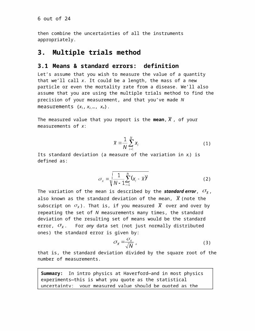
3.1 Means & standard errors: definitionLet’s assume that you wish to measure the value of a quantity that we’ll call x. It could be a length, the mass of a new particle or even the mortality rate from a disease. We’ll also assume that you are using the multiple trials method to find the precision of your measurement, and that you’ve made N measurements {x1, x2,…, xN}.

The measured value that you report is the mean, , of your measurements of x:

(1)

Its standard deviation (a measure of the variation in xi) is defined as:

(2)

The variation of the mean is described by the standard error, , also known as the standard

deviation of the mean, (note the subscript on ). That is, if you measured over and over by

repeating the set of N measurements many times, the standard deviation of the resulting set of

means would be the standard error, . For any data set (not just normally distributed ones) the

standard error is given by:

, (3)

that is, the standard deviation divided by the square root of the number of measurements.

Summary: In intro physics at Haverford—and in most physics experiments—this is what you quote as the statistical uncertainty: your measured value should be quoted as the mean ± the standard error: .

5 out of 15

3.2 How to compute means and standard errors of a measurement

Enter your data into a column of a spreadsheet using a program like Origin or Excel, and then use either program to compute the mean and standard error. Keep all significant figures in your original data and in your calculations at this step.

Origin has handy built-in statistics calculations on columns. You can select a column of data, and then choose from the top menu Statistics Descriptive Statistics Statistic on Columns, to automatically calculate these values. You can also right-click on the column to get these same options.

Excel does not have a function for the standard error, oddly enough, so you have to calculate the standard deviation (using the STDEV function) and divide by square root N; the mean is just given by the AVERAGE function.

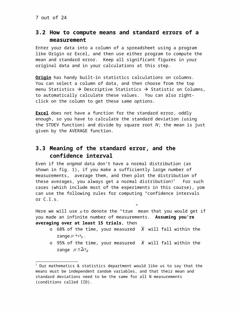
3.3 Meaning of the standard error, and the confidence intervalEven if the original data don’t have a normal distribution (as shown in fig. 1), if you make a sufficiently large number of measurements, average them, and then plot the distribution of these averages, you always get a normal distribution!1 For such cases (which include most of the experiments in this course), you can use the following rules for computing “confidence intervals” or C.I.s.

Here we will use to denote the “true” mean that you would get if you made an infinite number of measurements. Assuming you’re averaging over at least 15 trials, then

o 68% of the time, your measured will fall within the range .

o 95% of the time, your measured will fall within the range

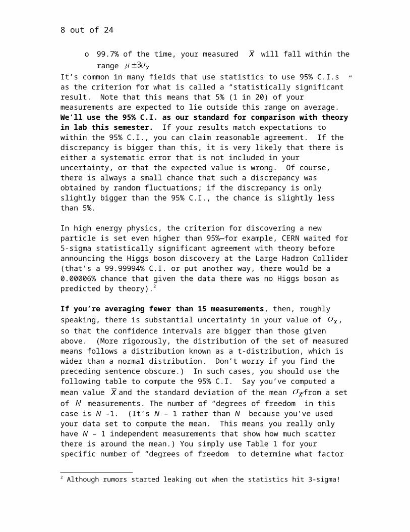
o 99.7% of the time, your measured will fall within the range

It’s common in many fields that use statistics to use 95% C.I.s as the criterion for what is called a “statistically significant” result. Note that this means that 5% (1 in 20) of your measurements are expected to lie outside this range on average. We’ll use the 95% C.I. as our standard for comparison with theory in lab this semester. If your results match expectations to within the 95% C.I., you can claim reasonable agreement. If the discrepancy is bigger than this, it is very likely that there is either a systematic error that is not included in your uncertainty, or that the expected value is wrong. Of course, there is always a small chance that such a discrepancy was obtained by random fluctuations; if the discrepancy is only slightly bigger than the 95% C.I., the chance is slightly less than 5%.

In high energy physics, the criterion for discovering a new particle is set even higher than 95%—for example, CERN waited for 5-sigma statistically significant agreement with theory before announcing the Higgs boson discovery at the Large Hadron Collider (that’s a 99.99994% C.I. or put another way, there would be a 0.00006% chance that given the data there was no Higgs boson as predicted by theory).2

1 Our mathematics & statistics department would like us to say that the means must be independent random variables, and that their mean and standard deviations need to be the same for all N measurements (conditions called IID).2 Although rumors started leaking out when the statistics hit 3-sigma!

6 out of 15

If you’re averaging fewer than 15 measurements, then, roughly speaking, there is substantial

uncertainty in your value of , so that the confidence intervals are bigger than those given

above. (More rigorously, the distribution of the set of measured means follows a distribution known as a t-distribution, which is wider than a normal distribution. Don’t worry if you find the preceding sentence obscure.) In such cases, you should use the following table to compute the

95% C.I. Say you’ve computed a mean value and the standard deviation of the mean from

a set of measurements. The number of “degrees of freedom” in this case is N -1. (It’s N – 1 rather than N because you’ve used your data set to compute the mean. This means you really only have N – 1 independent measurements that show how much scatter there is around the mean.) You simply use Table 1 for your specific number of “degrees of freedom” to determine

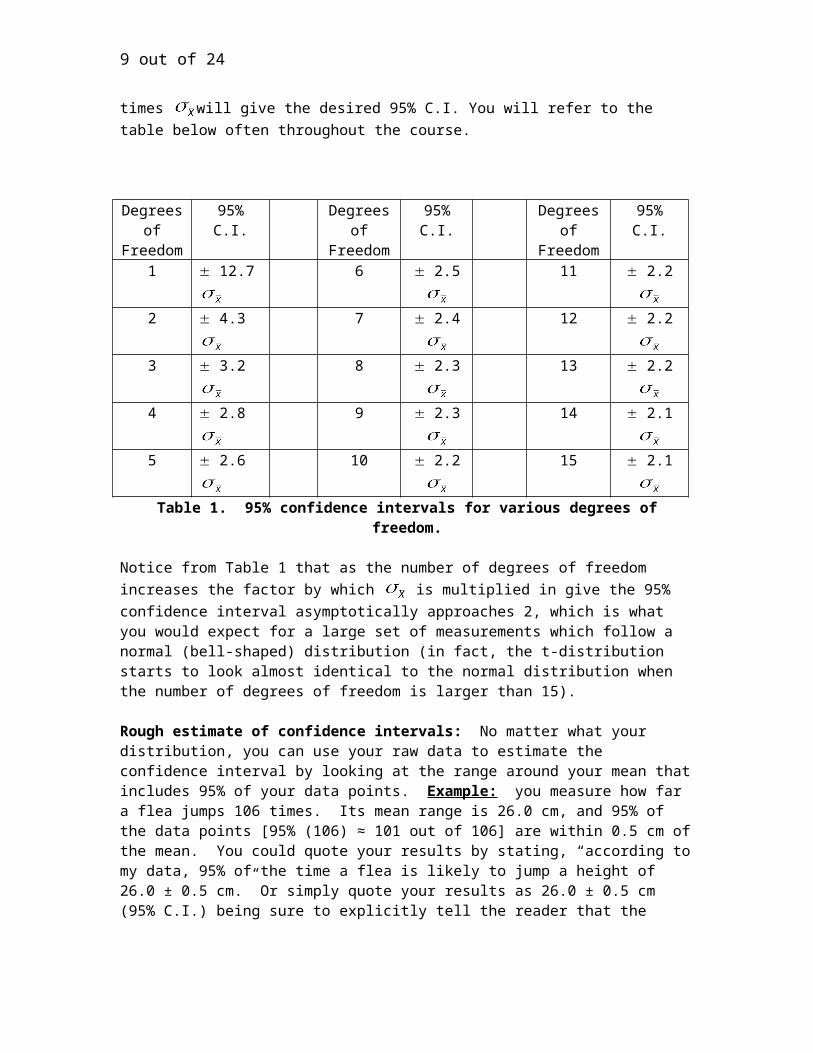
what factor times will give the desired 95% C.I. You will refer to the table below often

throughout the course.

Degrees of Freedom

95% C.I. Degrees of Freedom

95% C.I. Degrees of Freedom

95% C.I.

1 12.7 6 2.5 11 2.22 4.3 7 2.4 12 2.23 3.2 8 2.3 13 2.24 2.8 9 2.3 14 2.15 2.6 10 2.2 15 2.1

Table 1. 95% confidence intervals for various degrees of freedom.

Notice from Table 1 that as the number of degrees of freedom increases the factor by which

is multiplied in give the 95% confidence interval asymptotically approaches 2, which is what you would expect for a large set of measurements which follow a normal (bell-shaped) distribution (in fact, the t-distribution starts to look almost identical to the normal distribution when the number of degrees of freedom is larger than 15).

Rough estimate of confidence intervals: No matter what your distribution, you can use your raw data to estimate the confidence interval by looking at the range around your mean that includes 95% of your data points. Example: you measure how far a flea jumps 106 times. Its mean range is 26.0 cm, and 95% of the data points [95% (106) ≈ 101 out of 106] are within 0.5 cm of the mean. You could quote your results by stating, “according to my data, 95% of the time a flea is likely to jump a height of 26.0 ± 0.5 cm.” Or simply quote your results as 26.0 ± 0.5 cm (95% C.I.) being sure to explicitly tell the reader that the interval you are giving is a 95% confidence interval by writing out the “95% C.I.” in parentheses.

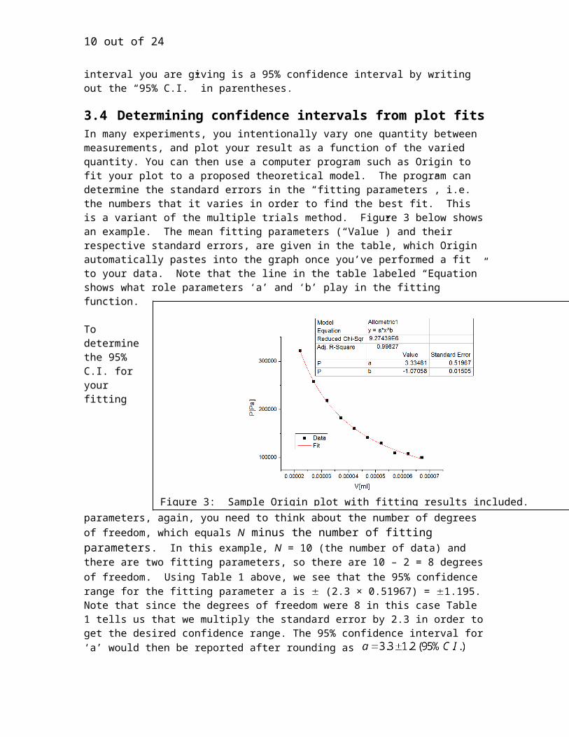
3.4 Determining confidence intervals from plot fitsIn many experiments, you intentionally vary one quantity between measurements, and plot your result as a function of the varied quantity. You can then use a computer program such as Origin to fit your plot to a proposed theoretical model. The program can determine the standard errors in the “fitting parameters”, i.e. the numbers that it varies in order to find the best fit. This is a variant of the multiple trials method. Figure 3 below shows an example. The mean fitting parameters (“Value”) and their respective standard errors, are given in the table, which Origin

7 out of 15

automatically pastes into the graph once you’ve performed a fit to your data. Note that the line in the table labeled “Equation” shows what role parameters ‘a’ and ‘b’ play in the fitting function.

To determine the 95% C.I. for your fitting parameters, again, you need to think about the number of degrees of freedom, which equals N minus the number of fitting parameters. In this example, N = 10 (the number of data) and there are two fitting parameters, so there are 10 – 2 = 8 degrees of freedom. Using Table 1 above, we see that the 95% confidence range for the fitting parameter a is (2.3 × 0.51967) = 1.195. Note that since the degrees of freedom were 8 in this case Table 1 tells us that we multiply the standard error by 2.3 in order to get the desired confidence range. The 95% confidence interval for ‘a’ would then be reported after rounding as

(see subsection 6.1 below on the rules for rounding measured values and their uncertainties).

4 Instrumental uncertainty method

4.1 Combining uncertainties from imprecision and inaccuracyThe uncertainty in the reading from a particular instrument comes both from lack of precision and lack of accuracy. In the most sophisticated treatments of uncertainty, these are handled separately. However, in this course we will combine them into a single uncertainty, as is done in most scientific papers. (There is one exception, which we’ll discuss at the end of this section.) Following standard practice, we will call this uncertainty ; this plays the same role that

does for the multiple trials method.

4.2 Confidence interval for the instrumental uncertainty method

The 95% confidence interval is 2 , and the 99.7% confidence interval is 3 .

Figure 3: Sample Origin plot with fitting results included.

8 out of 15

4.3 Determining the total uncertainty of an instrument

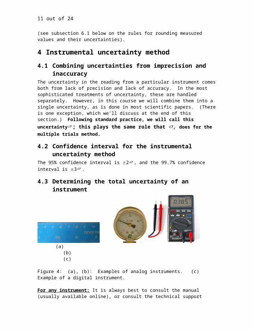
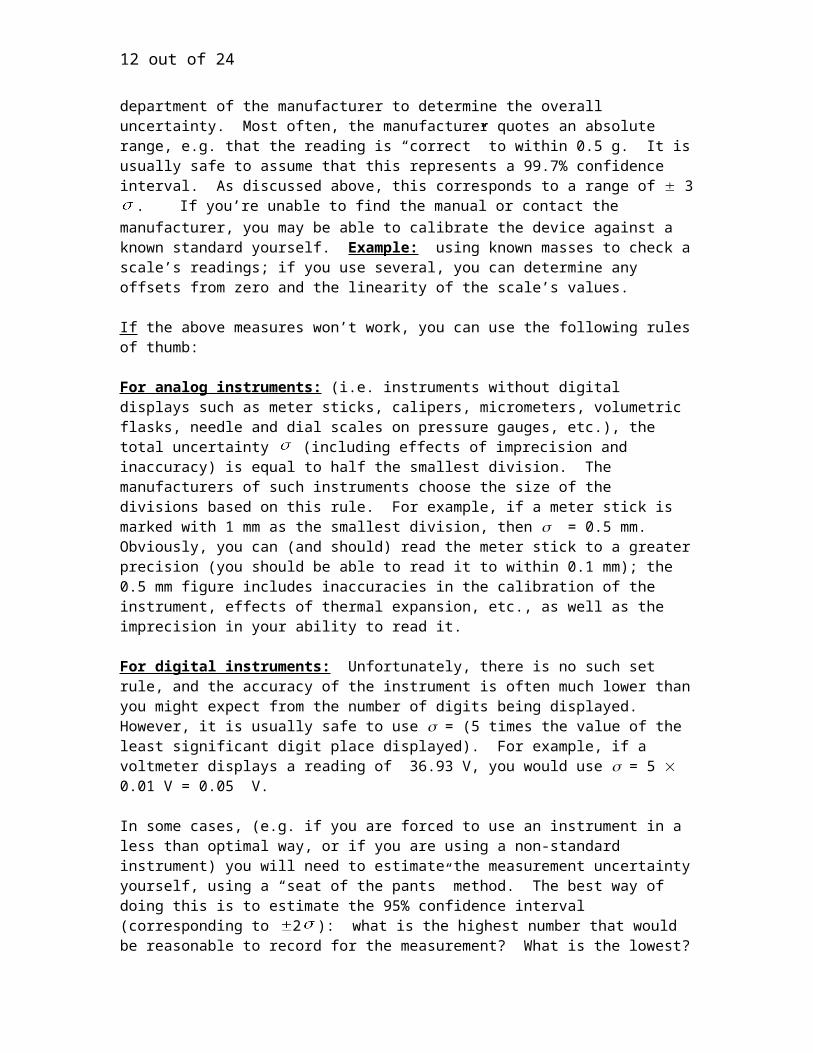
(a) (b) (c)

Figure 4: (a), (b): Examples of analog instruments. (c) Example of a digital instrument.

For any instrument: It is always best to consult the manual (usually available online), or consult the technical support department of the manufacturer to determine the overall uncertainty. Most often, the manufacturer quotes an absolute range, e.g. that the reading is “correct” to within 0.5 g. It is usually safe to assume that this represents a 99.7% confidence interval. As discussed above, this corresponds to a range of 3 . If you’re unable to find the manual or contact the manufacturer, you may be able to calibrate the device against a known standard yourself. Example: using known masses to check a scale’s readings; if you use several, you can determine any offsets from zero and the linearity of the scale’s values.

If the above measures won’t work, you can use the following rules of thumb:

For analog instruments: (i.e. instruments without digital displays such as meter sticks, calipers, micrometers, volumetric flasks, needle and dial scales on pressure gauges, etc.), the total uncertainty (including effects of imprecision and inaccuracy) is equal to half the smallest division. The manufacturers of such instruments choose the size of the divisions based on this rule. For example, if a meter stick is marked with 1 mm as the smallest division, then = 0.5 mm. Obviously, you can (and should) read the meter stick to a greater precision (you should be able to read it to within 0.1 mm); the 0.5 mm figure includes inaccuracies in the calibration of the instrument, effects of thermal expansion, etc., as well as the imprecision in your ability to read it.

For digital instruments: Unfortunately, there is no such set rule, and the accuracy of the instrument is often much lower than you might expect from the number of digits being displayed. However, it is usually safe to use = (5 times the value of the least significant digit place displayed). For example, if a voltmeter displays a reading of 36.93 V, you would use = 5 0.01 V = 0.05 V.

In some cases, (e.g. if you are forced to use an instrument in a less than optimal way, or if you are using a non-standard instrument) you will need to estimate the measurement uncertainty yourself, using a “seat of the pants” method. The best way of doing this is to estimate the 95% confidence interval (corresponding to 2 ): what is the highest number that would be reasonable to record for the measurement? What is the lowest? This range corresponds approximately to the 95% confidence interval. The span of this interval, from highest to lowest, is equal to 4 (i.e. 2 ).

9 out of 15

5 Propagation of errors: the uncertainty of a computed quantity

Important note on notation: The notation used in this section assumes you’ve used the multiple trials method. If instead you’ve used the instrumental

uncertainty method, simply substitute for .

5.1 Exact and approximate expressions for the uncertainty in a calculated quantity

Often you want to use the mean values and the uncertainty of measured quantities to compute an interesting physical quantity. For example, we can measure the ratio of charge to mass of an elementary particle by bending its path into an orbit using a strong magnet. The radius of that orbit depends on many measurable physical variables. How do we get the uncertainty of the calculated value? Assume we want to compute f(x) using measured values of x. Our estimate for is , that is,

the function evaluated at the computed average value of x. We can compute the standard error

of exactly using:

(4)

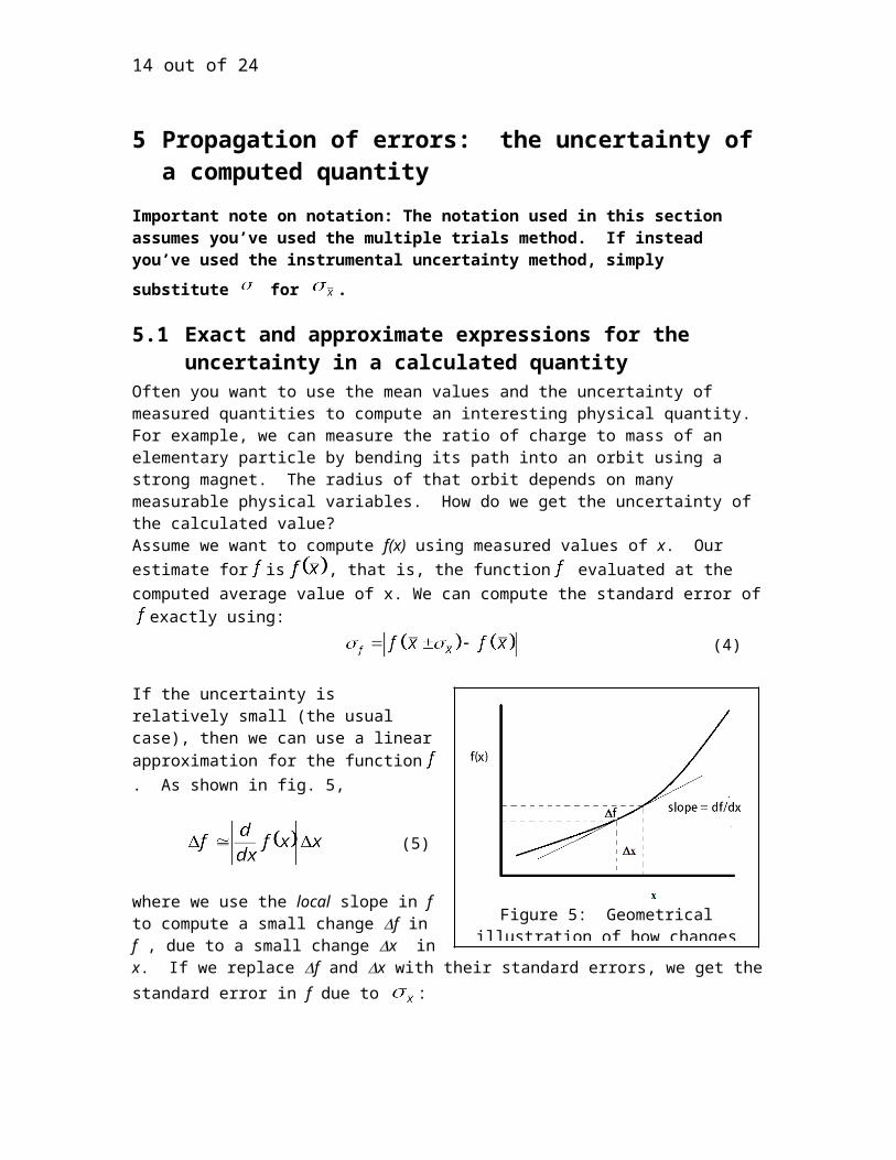
If the uncertainty is relatively small (the usual case), then we can use a linear approximation for the function . As shown in fig. 5,

(5)

where we use the local slope in f to compute a small change f in f , due to a small change x in x. If we replace f and x with their standard errors, we get the standard error in f due to :

(6)

5.2 Combining uncertainties arising from multiple variablesWhat if depends on more than one measured quantity, e.g. if depends on both x and y? In that case, assuming the variations in x and y are independent of each other, we can use equations similar to (6) to find the variation in that would result from each uncertainty:

and .

Figure 5: Geometrical illustration of how changes in f (x) relate to slope and x.

10 out of 15

The partial derivative means we take the derivative of f(x,y) with respect to x while

holding y constant. We could also use the more exact expressions (similar to equation 4):

and

To find the total uncertainty for , we cannot just add the two uncertainties due to x and y, since x is not always high when y is also high. Instead, we can derive a general relationship for their combined effect on . This uses a result from statistics that is similar to the Pythagorean theorem, called adding in quadrature. This result is generally true as long as x, y and any other variables (hence the + …) vary independently of each other:

(7)

In the calculus approximation this becomes:

(8)

Tips: If your calculated quantity will have a large variation when you compute it using your

measured uncertainty, you must use the exact formula (e.g. equation (4)) for the calculated uncertainty.

If your calculated quantity will vary by only a small amount, the approximate calculus-based formulas (e.g. equation (8)) should suffice.

The exact formula is always correct, so if it’s a bother to compute derivatives, it’s always OK to use that instead of the calculus-based approximations.

5.3 Sample calculationsNow suppose that you calculate a quantity f (say, the speed of light) that depends on two measured quantities x and y. Let the uncertainty associated with the measurement of x be x and the uncertainty associated with the measurement of y be y. Example 1: f (x,y)= Ax ± By (addition or subtraction) If there is no uncertainty in either A or B, then:

Example 2: f (x,y)= Axy (multiplication) If there is no uncertainty in A, then:

This is easier to interpret if you divide both sides by f (x,y)= Axy:

11 out of 15

The fractional uncertainty in f(x,y) is the sum in quadrature of the fractional uncertainties in x and y. Example: If the uncertainty in x is 3% and that in y is 4%, then

It is easy to show that this rule of adding fractional uncertainties in quadrature also works for division, e.g. f (x,y)= Ax/y

Other useful examples: f (x)= Axn (powers of x) If there is no uncertainty in A or n, then:

f (x)= Aebx (exponential) If there is no uncertainty in A or b, then:

Dominant sources of uncertainty: In general uncertainties that are ≤ 1/3 of the largest uncertainties only increase the overall uncertainty by ≤ 5% and those ≤ 1/5 by ≤ 2%. Don’t fuss about measuring tiny uncertainties exactly! Pay attention to your dominant sources of uncertainty.

6 Reporting your resultsIn general when you are asked to report a measured quantity with uncertainty you should always

give the measured value, and the standard error and report as:

that is, you just quote the measured value plus or minus one factor of the standard error. For example, if your estimate for the length of a pendulum is = 12.32 cm and you estimate the

= 0.05 cm then when you are asked to report the length of the pendulum you would report:

Length of Pendulum: 12.32 0.05 cm

It will be understood that you are reporting one factor of the standard error after the symbol.

If you are reporting on a 95% confidence interval you must always be sure to state explicitly that this is the case. Using the example above, we would state the 95% confidence interval as:

Length of Pendulum: 12.32 0.10 cm (95% C.I.)

Where I’ve assumed a normal distribution of measurements and simply multiplied the standard error by 2 in order to get the desired confidence interval.

6.1 Significant figures, units & justificationsWhen you give your results, quote the uncertainty to one significant figure in lab unless the leading digit is 1, in which case you should retain two significant figures. Example: An uncertainty of 0.0539 would be expressed as ±0.05, while 0.0001569 would be ±0.00016.

12 out of 15

Round the measured quantity itself to the appropriate decimal place so its smallest significant figure has the same order of magnitude as the uncertainty. Example: Round 3.14 ± 0.2 m to 3.1 m ± 0.2 m.

However, when you do any calculations using measured values with uncertainties (such as the propagation of errors mentioned in the previous section) retain one extra figure beyond your valid number of significant figures and round to the correct number of significant figures after the calculation.

When you see a value quoted to a certain number of significant figures, you can assume that it is known to at best half the lowest significant figure. Example: If the mass of the electron is given as 9.11 × 10-31 kg, that implies its value is (9.110 ± 0.005) × 10-31 kg. (99.7% C.I.) (In fact, it’s known to many more significant figures, but that’s all you can count on given only 3 significant figures!)

Be sure to include units in both the measured quantity and its uncertainty. Example: g = 9.82 ± 0.02 m/s2 or g = (9.82 ± 0.02) m/s2 or g = 9.82 m/s2 ± 0.02 m/s2 are all acceptable.

Just as you need to explain how you measured a quantity, you need to explain how you determined the uncertainty. You can’t just give a value: you must explain your reasoning and any measurements that went into finding them.

6.2 How to describe confidence intervalsYou must be careful to use the term “confidence interval” properly. Remember the meaning of the confidence interval: If you repeat your experiment many times, then 95% of your final results would fall within the 95% C.I., and 5% of your results would fall outside it based solely on statistical fluctuations.

For example, say you measure the gravitational acceleration to be (9.83 0.01) m/s2 so that we have (9.83 0.02) m/s2 as the 95% C.I. The expected result of 9.81 m/s2 is right at the edge of the 95% C.I. It would be correct to say, “The expected value is within the 95% confidence range of my experiment, indicating a reasonable level of agreement.” However, because the expected value is right at the edge of the C.I., it would also be correct to say, “There is only a 5% chance that the discrepancy between my measurement and the expected value was caused by fluctuations and inaccuracies that are included in my uncertainty analysis.” It would be wrong to say, “My results show with 95% confidence that the expected value is correct.” After all, if your measured value was instead (9.84 0.01) m/s2 and you had chosen instead to quote a 99.7% C.I. then again the expected value is just at the edge of this C.I.—i.e., note the discrepancy is greater than above —you would certainly not say, “My results show with 99.7% confidence that the expected value is correct.” In fact, your results being on the edge of a 99.7% confidence interval would only occur 0.3% of the time (assuming no unaccounted for errors in accuracy or precision) and this is surely not a situation in which you should be “99.7% confident that your results are correct”. In this case, there is 99.7% chance that the discrepancy was caused by a systematic error in your experiment that is not accounted for in your uncertainty analysis, or that the expected value is wrong.

just barely agree to within the 95% C.I. Adapted from http://scienceblogs.com/cognitivedaily/2008/07/31/most-researchers-dont-understa-1/

13 out of 15

6.3 Hypothesis testing: How to compare two values using their uncertainties

In experimental science, your goal is often to test agreement between a measured and theoretical value, or between two different experimental values. If you’re comparing a value that has a relatively high uncertainty (e.g. your experimental result) to a value with a very low uncertainty (e.g. an accepted value), then it’s easy; you just use the confidence intervals for the larger uncertainty as described above, assuming that the quantity with lower uncertainty is exact. This works very well if the uncertainty in one quantity is at least 5 times bigger than the uncertainty in the other. However, if you’re comparing two quantities that have a similar level of uncertainty, the situation is a little more complicated.

Say you wish to compare two estimates for x, either from two different measurements (e.g., energy before and after a collision), or a measurement and a calculation:

First value:

Second value: (Here we’re quoting 95% C.I.s.) When can we say that the two values agree to within uncertainties? This is equivalent to asking whether the 95% confidence range for the difference

includes 0. We can compute the uncertainty of just as for any other

calculated value (as described above in subsection 5.3 Example 1), using and , yielding

.

We multiply this by the appropriate constant (as described above) to get the desired confidence interval. Again, remember that, the bigger the confidence range you would have to use to include 0, the worse the agreement is. For example, if 0 is just outside the 99.7% confidence range, then it is 99.7% likely that there is an unaccounted-for systematic error.

Interesting special case: If , then

1.4 .

It’s good to be able to visualize what agreement and disagreement look like graphically. We’ll assume either that we’re using the multiple trials method with at least 15 trials, or that we’re using the instrumental uncertainty method, so that the 95% C.I. for the difference is given by . Figure 6 illustrates the minimal requirement for

agreement between and within the 95% C.I. The

95% C.I. error bars shown in the figure for each point are . If the two means are separated by more than

, then they disagree with

95% confidence. The two points shown in Figure 6 are separated by exactly this amount, so their

error bars overlap by an amount of 0.6*( ) = 1.2 . Even if the individual 95% C.I. of and

overlap by some amount up to and less than 1.2 , there is 95% likelihood of a real

discrepancy!3

3 Scientists are surprised by this too, and most get it wrong! http://isites.harvard.edu/fs/docs/icb.topic477909.files/misunderstood_confidence.pdf

14 out of 15

6.4 Discussing your results & their uncertaintiesWhether your data agree with expectations or not, you should always briefly discuss the major sources of error and uncertainty. Recall that a source of error is defined as some respect in which the experiment might have been performed better with the existing equipment, or some respect in which the theory could have described the experiment more accurately, while uncertainty arises from the limitations of the equipment. For example, accidentally pushing on the pendulum bob as you let it go would be a source of experimental error, and ignoring air resistance would be a source of theoretical error, while the uncertainty in reading a measurement off a meter stick would be a source of experimental uncertainty.

Usually there will be from one to three sources of error that are much more important than the rest, and your discussion should focus on these. These may include both simplifications made in the theory (for instance, neglecting air resistance), and experimental sources of error, such as the difficulty in determining the exact apex of a trajectory. Be as specific as possible. Vague terms such as "human error" are completely unacceptable. For each source of error or uncertainty, discuss the direction in which it may have altered your results (i.e. whether it would have made your final result larger or smaller). If your results differ from expectation, discuss whether this direction helps to explain the discrepancy, and whether the magnitude of the source of error or uncertainty is large enough to account for the discrepancy. We do not expect a fully quantitative discussion, but you should be able to give a qualitative idea. For example, in an experiment which checks the conservation of mechanical energy in a pendulum, air resistance might affect the kinetic energy by a few percent, but definitely could not account for a discrepancy as large as 25%. Note that, unlike statistical (random) uncertainties, most sources of experimental or theoret-ical error do have an associated direction.

7 Doing your best work in lab Do a trial measurement to map out your procedure and likely measured values, and to

organize your workspace. Understand how to operate all equipment thoroughly. You can only get really good data

if you have a deep understanding of your equipment. Plan how to record your data before you start your experiment: organize your lab

notebook, spreadsheet, and/or report form; write down everything you can before you start; include units and scales (mV or V?); write neatly, organizing different measurements clearly.

Check the obvious: everything is plugged in, mechanical parts aren’t wobbly, wires and connectors are firmly attached, ground wires go to ground, polarities of electrical wires are correct (positive to positive), all power supplies start at their lowest (and safest) values before turned on, etc.

Think! It takes a lot of careful thought to be a good experimentalist. Make sure you understand what you’re doing; ask questions if you need to.

Do as much of the analysis as you can before leaving lab. That way, if you have questions, you can ask your instructor.

8 Tips for taking data: How many points to collect and where to measure them

Before you start your experiment, carefully design your data-taking plan. Space your data out over the range of independent variables sensibly—uniformly for linear

variations, but non-uniformly for other functional forms.

15 out of 15

Don’t waste time taking excessive data points in a region with no change, and too few in a region where the results change dramatically.

Plot your data as you go to check that you are achieving a good distribution of measured values.

One good plan: measure the highest and lowest values first, then map out the regions in between. (Don’t clump many data points around one limited region of parameters.) Vary your independent variables by wide amounts, not tiny steps, and plot as you go!

Remember that any function looks like a straight line over sufficiently small intervals. Your planned range of data taking should actually probe the relevant functional behavior, not just a localized slope or curvature in one neighborhood.

9 Mistakes: What to do when things go wrongWhat happens when you or your partner goof up, or a piece of equipment malfunctions, so your data points are just plain wrong? Not when they return unexpected answers—that might even be the point of the lab!

You used the equipment wrong. You forgot to take an important measurement required to understand your results. You forgot to write down an important piece of information. And so on.

First, calm down. You are in excellent company—this happened to Albert Einstein, too. At least you’re not going to make it into the history books by messing up in this lab class!

The rule is simple: You must not report incorrect data without comment when you know you have messed up a measurement, however innocently or unavoidably. If you can’t fix it, you need to document what went wrong honestly. We’ll respect your integrity for doing so.

If you have time, redo the experiment. Sometimes you can report only part of what was desired. In many cases it is possible to go back after the fact and fix the problem. Perhaps you can recalibrate your measuring device before its behavior changes. Or you can perform another measurement to correct for the mistake you made. Or you can resume a measurement, taking special care to be sure you really are able to put the two data sets together. Consult with us about what to do if you’re not sure what the next step ought to be. We are here to help you trouble-shoot. In fact, that’s often when you learn the most!

10 A final commentThis document should prove adequate for the cases you encounter in the first year of introductory physics. The textbooks on reserve have more information if you ever need it for your senior thesis.4

4 See Chapter 2, John R. Taylor, An Introduction to Error Analysis, University Science Books, second edition, 1997.