Searching for stochastic gravitational waves using data fromthe two colocated LIGO Hanford detectors

J. Aasi,1 J. Abadie,1 B. P. Abbott,1 R. Abbott,1 T. Abbott,2 M. R. Abernathy,1 T. Accadia,3 F. Acernese,4,5 C. Adams,6

T. Adams,7 P. Addesso,8 R. X. Adhikari,1 C. Affeldt,9 M. Agathos,10 N. Aggarwal,11 O. D. Aguiar,12 P. Ajith,1

B. Allen,9,13,14 A. Allocca,15,16 E. Amador Ceron,13 D. Amariutei,17 R. A. Anderson,1 S. B. Anderson,1 W. G. Anderson,13

K. Arai,1 M. C. Araya,1 C. Arceneaux,18 J. Areeda,19 S. Ast,14 S. M. Aston,6 P. Astone,20 P. Aufmuth,14 C. Aulbert,9

L. Austin,1 B. E. Aylott,21 S. Babak,22 P. T. Baker,23 G. Ballardin,24 S.W. Ballmer,25 J. C. Barayoga,1 D. Barker,26

S. H. Barnum,11 F. Barone,4,5 B. Barr,27 L. Barsotti,11 M. Barsuglia,28 M. A. Barton,26 I. Bartos,29 R. Bassiri,30,27

A. Basti,31,16 J. Batch,26 J. Bauchrowitz,9 Th. S. Bauer,10 M. Bebronne,3 B. Behnke,22 M. Bejger,32 M. G. Beker,10

A. S. Bell,27 C. Bell,27 I. Belopolski,29 G. Bergmann,9 J. M. Berliner,26 D. Bersanetti,33,34 A. Bertolini,10 D. Bessis,35

J. Betzwieser,6 P. T. Beyersdorf,36 T. Bhadbhade,30 I. A. Bilenko,37 G. Billingsley,1 J. Birch,6 S. Biscans,11 M. Bitossi,16

M. A. Bizouard,38 E. Black,1 J. K. Blackburn,1 L. Blackburn,39 D. Blair,40 M. Blom,10 O. Bock,9 T. P. Bodiya,11 M. Boer,41

C. Bogan,9 C. Bond,21 F. Bondu,42 L. Bonelli,31,16 R. Bonnand,43 R. Bork,1 M. Born,9 V. Boschi,16 S. Bose,44 L. Bosi,45

J. Bowers,2 C. Bradaschia,16 P. R. Brady,13 V. B. Braginsky,37 M. Branchesi,46,47 C. A. Brannen,44 J. E. Brau,48 J. Breyer,9

T. Briant,49 D. O. Bridges,6 A. Brillet,41 M. Brinkmann,9 V. Brisson,38 M. Britzger,9 A. F. Brooks,1 D. A. Brown,25

D. D. Brown,21 F. Brückner,21 T. Bulik,50 H. J. Bulten,51,10 A. Buonanno,52 D. Buskulic,3 C. Buy,28 R. L. Byer,30

L. Cadonati,53 G. Cagnoli,43 J. Calderón Bustillo,54 E. Calloni,55,5 J. B. Camp,39 P. Campsie,27 K. C. Cannon,56 B. Canuel,24

J. Cao,57 C. D. Capano,52 F. Carbognani,24 L. Carbone,21 S. Caride,58 A. Castiglia,59 S. Caudill,13 M. Cavaglià,18

F. Cavalier,38 R. Cavalieri,24 G. Cella,16 C. Cepeda,1 E. Cesarini,60 R. Chakraborty,1 T. Chalermsongsak,1 S. Chao,61

P. Charlton,62 E. Chassande-Mottin,28 X. Chen,40 Y. Chen,63 A. Chincarini,34 A. Chiummo,24 H. S. Cho,64 J. Chow,65

N. Christensen,66 Q. Chu,40 S. S. Y. Chua,65 S. Chung,40 G. Ciani,17 F. Clara,26 D. E. Clark,30 J. A. Clark,53 F. Cleva,41

E. Coccia,67,60 P.-F. Cohadon,49 A. Colla,68,20 M. Colombini,45 M. Constancio, Jr.,12 A. Conte,68,20 D. Cook,26 T. R. Corbitt,2

M. Cordier,36 N. Cornish,23 A. Corsi,69 C. A. Costa,12 M.W. Coughlin,70 J.-P. Coulon,41 S. Countryman,29 P. Couvares,25

D. M. Coward,40 M. Cowart,6 D. C. Coyne,1 K. Craig,27 J. D. E. Creighton,13 T. D. Creighton,35 S. G. Crowder,71

A. Cumming,27 L. Cunningham,27 E. Cuoco,24 K. Dahl,9 T. Dal Canton,9 M. Damjanic,9 S. L. Danilishin,40 S. D’Antonio,60

K. Danzmann,9,14 V. Dattilo,24 B. Daudert,1 H. Daveloza,35 M. Davier,38 G. S. Davies,27 E. J. Daw,72 R. Day,24 T. Dayanga,44

G. Debreczeni,73 J. Degallaix,43 E. Deleeuw,17 S. Deléglise,49 W. Del Pozzo,10 T. Denker,9 T. Dent,9 H. Dereli,41

V. Dergachev,1 R. T. DeRosa,2 R. De Rosa,55,5 R. DeSalvo,74 S. Dhurandhar,75 M. Díaz,35 A. Dietz,18 L. Di Fiore,5

A. Di Lieto,31,16 I. Di Palma,9 A. Di Virgilio,16 K. Dmitry,37 F. Donovan,11 K. L. Dooley,9 S. Doravari,6 M. Drago,76,77

R. W. P. Drever,78 J. C. Driggers,1 Z. Du,57 J.-C. Dumas,40 S. Dwyer,26 T. Eberle,9 M. Edwards,7 A. Effler,2 P. Ehrens,1

J. Eichholz,17 S. S. Eikenberry,17 G. Endrőczi,73 R. Essick,11 T. Etzel,1 K. Evans,27 M. Evans,11 T. Evans,6

M. Factourovich,29 V. Fafone,67,60 S. Fairhurst,7 Q. Fang,40 B. Farr,79 W. Farr,79 M. Favata,80 D. Fazi,79 H. Fehrmann,9

D. Feldbaum,17,6 I. Ferrante,31,16 F. Ferrini,24 F. Fidecaro,31,16 L. S. Finn,81 I. Fiori,24 R. Fisher,25 R. Flaminio,43 E. Foley,19

S. Foley,11 E. Forsi,6 N. Fotopoulos,1 J.-D. Fournier,41 S. Franco,38 S. Frasca,68,20 F. Frasconi,16 M. Frede,9 M. Frei,59

Z. Frei,82 A. Freise,21 R. Frey,48 T. T. Fricke,9 P. Fritschel,11 V. V. Frolov,6 M.-K. Fujimoto,83 P. Fulda,17 M. Fyffe,6 J. Gair,70

L. Gammaitoni,84,45 J. Garcia,26 F. Garufi,55,5 N. Gehrels,39 G. Gemme,34 E. Genin,24 A. Gennai,16 L. Gergely,85 S. Ghosh,44

J. A. Giaime,2,6 S. Giampanis,13 K. D. Giardina,6 A. Giazotto,16 S. Gil-Casanova,54 C. Gill,27 J. Gleason,17 E. Goetz,9

R. Goetz,17 L. Gondan,82 G. González,2 N. Gordon,27 M. L. Gorodetsky,37 S. Gossan,63 S. Goßler,9 R. Gouaty,3 C. Graef,9

P. B. Graff,39 M. Granata,43 A. Grant,27 S. Gras,11 C. Gray,26 R. J. S. Greenhalgh,86 A. M. Gretarsson,87 C. Griffo,19

H. Grote,9 K. Grover,21 S. Grunewald,22 G. M. Guidi,46,47 C. Guido,6 K. E. Gushwa,1 E. K. Gustafson,1 R. Gustafson,58

B. Hall,44 E. Hall,1 D. Hammer,13 G. Hammond,27 M. Hanke,9 J. Hanks,26 C. Hanna,88 J. Hanson,6 J. Harms,1 G. M. Harry,89

I. W. Harry,25 E. D. Harstad,48 M. T. Hartman,17 K. Haughian,27 K. Hayama,83 J. Heefner,1 A. Heidmann,49 M. Heintze,17,6

H. Heitmann,41 P. Hello,38 G. Hemming,24 M. Hendry,27 I. S. Heng,27 A.W. Heptonstall,1 M. Heurs,9 S. Hild,27 D. Hoak,53

K. A. Hodge,1 K. Holt,6 T. Hong,63 S. Hooper,40 T. Horrom,90 D. J. Hosken,91 J. Hough,27 E. J. Howell,40 Y. Hu,27 Z. Hua,57

V. Huang,61 E. A. Huerta,25 B. Hughey,87 S. Husa,54 S. H. Huttner,27 M. Huynh,13 T. Huynh-Dinh,6 J. Iafrate,2

D. R. Ingram,26 R. Inta,65 T. Isogai,11 A. Ivanov,1 B. R. Iyer,92 K. Izumi,26 M. Jacobson,1 E. James,1 H. Jang,93 Y. J. Jang,79

P. Jaranowski,94 F. Jiménez-Forteza,54 W.W. Johnson,2 D. I. Jones,95 D. Jones,26 R. Jones,27 R. J. G. Jonker,10 L. Ju,40

Haris K.,96 P. Kalmus,1 V. Kalogera,79 S. Kandhasamy,18,71,* G. Kang,93 J. B. Kanner,39 M. Kasprzack,38,24 R. Kasturi,97

E. Katsavounidis,11 W. Katzman,6 H. Kaufer,14 K. Kaufman,63 K. Kawabe,26 S. Kawamura,83 F. Kawazoe,9 F. Kéfélian,41

D. Keitel,9 D. B. Kelley,25 W. Kells,1 D. G. Keppel,9 A. Khalaidovski,9 F. Y. Khalili,37 E. A. Khazanov,98 B. K. Kim,93

C. Kim,99,93 K. Kim,100 N. Kim,30 W. Kim,91 Y.-M. Kim,64 E. King,91 P. J. King,1 D. L. Kinzel,6 J. S. Kissel,11

S. Klimenko,17 J. Kline,13 S. Koehlenbeck,9 K. Kokeyama,2 V. Kondrashov,1 S. Koranda,13 W. Z. Korth,1 I. Kowalska,50

D. Kozak,1 A. Kremin,71 V. Kringel,9 B. Krishnan,9 A. Królak,101,102 C. Kucharczyk,30 S. Kudla,2 G. Kuehn,9 A. Kumar,103

D. Nanda Kumar,17 P. Kumar,25 R. Kumar,27 R. Kurdyumov,30 P. Kwee,11 M. Landry,26 B. Lantz,30 S. Larson,104

PHYSICAL REVIEW D 91, 022003 (2015)

1550-7998=2015=91(2)=022003(22) 022003-1 © 2015 American Physical Society

P. D. Lasky,105 C. Lawrie,27 A. Lazzarini,1 P. Leaci,22 E. O. Lebigot,57 C.-H. Lee,64 H. K. Lee,100 H. M. Lee,99 J. J. Lee,19

J. Lee,11 M. Leonardi,76,77 J. R. Leong,9 A. Le Roux,6 N. Leroy,38 N. Letendre,3 B. Levine,26 J. B. Lewis,1 V. Lhuillier,26

T. G. F. Li,10 A. C. Lin,30 T. B. Littenberg,79 V. Litvine,1 F. Liu,106 H. Liu,7 Y. Liu,57 Z. Liu,17 D. Lloyd,1 N. A. Lockerbie,107

V. Lockett,19 D. Lodhia,21 K. Loew,87 J. Logue,27 A. L. Lombardi,53 M. Lorenzini,67,60 V. Loriette,108 M. Lormand,6

G. Losurdo,47 J. Lough,25 J. Luan,63 M. J. Lubinski,26 H. Lück,9,14 A. P. Lundgren,9 J. Macarthur,27 E. Macdonald,7

B. Machenschalk,9 M. MacInnis,11 D. M. Macleod,7 F. Magana-Sandoval,19 M. Mageswaran,1 K. Mailand,1 E. Majorana,20

I. Maksimovic,108 V. Malvezzi,67,60 N. Man,41 G. M. Manca,9 I. Mandel,21 V. Mandic,71 V. Mangano,68,20 M. Mantovani,16

F. Marchesoni,109,45 F. Marion,3 S. Márka,29 Z. Márka,29 A. Markosyan,30 E. Maros,1 J. Marque,24 F. Martelli,46,47

L. Martellini,41 I. W. Martin,27 R. M. Martin,17 G. Martini,1 D. Martynov,1 J. N. Marx,1 K. Mason,11 A. Masserot,3

T. J. Massinger,25 F. Matichard,11 L. Matone,29 R. A. Matzner,110 N. Mavalvala,11 G. May,2 N. Mazumder,96 G. Mazzolo,9

R. McCarthy,26 D. E. McClelland,65 S. C. McGuire,111 G. McIntyre,1 J. McIver,53 D. Meacher,41 G. D. Meadors,58

M. Mehmet,9 J. Meidam,10 T. Meier,14 A. Melatos,105 G. Mendell,26 R. A. Mercer,13 S. Meshkov,1 C. Messenger,27

M. S. Meyer,6 H. Miao,63 C. Michel,43 E. Mikhailov,90 L. Milano,55,5 J. Miller,65 Y. Minenkov,60 C. M. F. Mingarelli,21

S. Mitra,75 V. P. Mitrofanov,37 G. Mitselmakher,17 R. Mittleman,11 B. Moe,13 M. Mohan,24 S. R. P. Mohapatra,25,59

F. Mokler,9 D. Moraru,26 G. Moreno,26 N. Morgado,43 T. Mori,83 S. R. Morriss,35 K. Mossavi,9 B. Mours,3

C. M. Mow-Lowry,9 C. L. Mueller,17 G. Mueller,17 S. Mukherjee,35 A. Mullavey,2 J. Munch,91 D. Murphy,29 P. G. Murray,27

A. Mytidis,17 M. F. Nagy,73 I. Nardecchia,67,60 T. Nash,1 L. Naticchioni,68,20 R. Nayak,112 V. Necula,17 I. Neri,84,45

M. Neri,33,34 G. Newton,27 T. Nguyen,65 E. Nishida,83 A. Nishizawa,83 A. Nitz,25 F. Nocera,24 D. Nolting,6

M. E. Normandin,35 L. K. Nuttall,7 E. Ochsner,13 J. O’Dell,86 E. Oelker,11 G. H. Ogin,1 J. J. Oh,113 S. H. Oh,113 F. Ohme,7

P. Oppermann,9 B. O’Reilly,6 W. Ortega Larcher,35 R. O’Shaughnessy,13 C. Osthelder,1 D. J. Ottaway,91 R. S. Ottens,17

J. Ou,61 H. Overmier,6 B. J. Owen,81 C. Padilla,19 A. Pai,96 C. Palomba,20 Y. Pan,52 C. Pankow,13 F. Paoletti,24,16

R. Paoletti,15,16 H. Paris,26 A. Pasqualetti,24 R. Passaquieti,31,16 D. Passuello,16 M. Pedraza,1 P. Peiris,59 S. Penn,97

A. Perreca,25 M. Phelps,1 M. Pichot,41 M. Pickenpack,9 F. Piergiovanni,46,47 V. Pierro,74 L. Pinard,43 B. Pindor,105

I. M. Pinto,74 M. Pitkin,27 J. Poeld,9 R. Poggiani,31,16 V. Poole,44 F. Postiglione,8 C. Poux,1 V. Predoi,7 T. Prestegard,71

L. R. Price,1 M. Prijatelj,9 S. Privitera,1 G. A. Prodi,76,77 L. Prokhorov,37 O. Puncken,35 M. Punturo,45 P. Puppo,20

V. Quetschke,35 E. Quintero,1 R. Quitzow-James,48 F. J. Raab,26 D. S. Rabeling,51,10 I. Rácz,73 H. Radkins,26 P. Raffai,29,82

S. Raja,114 G. Rajalakshmi,115 M. Rakhmanov,35 C. Ramet,6 P. Rapagnani,68,20 V. Raymond,1 V. Re,67,60 C. M. Reed,26

T. Reed,116 T. Regimbau,41 S. Reid,117 D. H. Reitze,1,17 F. Ricci,68,20 R. Riesen,6 K. Riles,58 N. A. Robertson,1,27 F. Robinet,38

A. Rocchi,60 S. Roddy,6 C. Rodriguez,79 M. Rodruck,26 C. Roever,9 L. Rolland,3 J. G. Rollins,1 J. D. Romano,35

R. Romano,4,5 G. Romanov,90 J. H. Romie,6 D. Rosińska,118,32 S. Rowan,27 A. Rüdiger,9 P. Ruggi,24 K. Ryan,26 F. Salemi,9

L. Sammut,105 V. Sandberg,26 J. Sanders,58 V. Sannibale,1 I. Santiago-Prieto,27 E. Saracco,43 B. Sassolas,43

B. S. Sathyaprakash,7 P. R. Saulson,25 R. Savage,26 R. Schilling,9 R. Schnabel,9,14 R. M. S. Schofield,48 E. Schreiber,9

D. Schuette,9 B. Schulz,9 B. F. Schutz,22,7 P. Schwinberg,26 J. Scott,27 S. M. Scott,65 F. Seifert,1 D. Sellers,6

A. S. Sengupta,119 D. Sentenac,24 V. Sequino,67,60 A. Sergeev,98 D. Shaddock,65 S. Shah,10,120 M. S. Shahriar,79 M. Shaltev,9

B. Shapiro,30 P. Shawhan,52 D. H. Shoemaker,11 T. L. Sidery,21 K. Siellez,41 X. Siemens,13 D. Sigg,26 D. Simakov,9

A. Singer,1 L. Singer,1 A. M. Sintes,54 G. R. Skelton,13 B. J. J. Slagmolen,65 J. Slutsky,9 J. R. Smith,19 M. R. Smith,1

R. J. E. Smith,21 N. D. Smith-Lefebvre,1 K. Soden,13 E. J. Son,113 B. Sorazu,27 T. Souradeep,75 L. Sperandio,67,60

A. Staley,29 E. Steinert,26 J. Steinlechner,9 S. Steinlechner,9 S. Steplewski,44 D. Stevens,79 A. Stochino,65 R. Stone,35

K. A. Strain,27 N. Straniero,43 S. Strigin,37 A. S. Stroeer,35 R. Sturani,46,47 A. L. Stuver,6 T. Z. Summerscales,121

S. Susmithan,40 P. J. Sutton,7 B. Swinkels,24 G. Szeifert,82 M. Tacca,28 D. Talukder,48 L. Tang,35 D. B. Tanner,17

S. P. Tarabrin,9 R. Taylor,1 A. P. M. ter Braack,10 M. P. Thirugnanasambandam,1 M. Thomas,6 P. Thomas,26 K. A. Thorne,6

K. S. Thorne,63 E. Thrane,1 V. Tiwari,17 K. V. Tokmakov,107 C. Tomlinson,72 A. Toncelli,31,16 M. Tonelli,31,16 O. Torre,15,16

C. V. Torres,35 C. I. Torrie,1,27 F. Travasso,84,45 G. Traylor,6 M. Tse,29 D. Ugolini,122 C. S. Unnikrishnan,115 H. Vahlbruch,14

G. Vajente,31,16 M. Vallisneri,63 J. F. J. van den Brand,51,10 C. Van Den Broeck,10 S. van der Putten,10 M. V. van der Sluys,79

J. van Heijningen,10 A. A. van Veggel,27 S. Vass,1 M. Vasúth,73 R. Vaulin,11 A. Vecchio,21 G. Vedovato,123 P. J. Veitch,91

J. Veitch,10 K. Venkateswara,124 D. Verkindt,3 S. Verma,40 F. Vetrano,46,47 A. Viceré,46,47 R. Vincent-Finley,111 J.-Y. Vinet,41

S. Vitale,11 S. Vitale,10 B. Vlcek,13 T. Vo,26 H. Vocca,84,45 C. Vorvick,26 W. D. Vousden,21 D. Vrinceanu,35 S. P. Vyachanin,37

A. Wade,65 L. Wade,13 M. Wade,13 S. J. Waldman,11 M. Walker,2 L. Wallace,1 Y. Wan,57 J. Wang,61 M. Wang,21 X. Wang,57

A. Wanner,9 R. L. Ward,65 M. Was,9 B. Weaver,26 L.-W. Wei,41 M. Weinert,9 A. J. Weinstein,1 R. Weiss,11 T. Welborn,6

L. Wen,40 P. Wessels,9 M. West,25 T. Westphal,9 K. Wette,9 J. T. Whelan,59 D. J. White,72 B. F. Whiting,17 S. Wibowo,13

K. Wiesner,9 C. Wilkinson,26 L. Williams,17 R. Williams,1 T. Williams,125 J. L. Willis,126 B. Willke,9,14 M. Wimmer,9

L. Winkelmann,9 W. Winkler,9 C. C. Wipf,11 H. Wittel,9 G. Woan,27 J. Worden,26 J. Yablon,79 I. Yakushin,6 H. Yamamoto,1

C. C. Yancey,52 H. Yang,63 D. Yeaton-Massey,1 S. Yoshida,125 H. Yum,79 M. Yvert,3 A. Zadrożny,101 M. Zanolin,87

J.-P. Zendri,123 F. Zhang,11 L. Zhang,1 C. Zhao,40 H. Zhu,81 X. J. Zhu,40 N. Zotov,116 M. E. Zucker,11 and J. Zweizig1

(LIGO Scientific Collaboration and Virgo Collaboration)

J. AASI et al. PHYSICAL REVIEW D 91, 022003 (2015)

022003-2

1LIGO—California Institute of Technology, Pasadena, California 91125, USA2Louisiana State University, Baton Rouge, Louisiana 70803, USA

3Laboratoire d’Annecy-le-Vieux de Physique des Particules (LAPP), Université de Savoie, CNRS/IN2P3,F-74941 Annecy-le-Vieux, France

4Università di Salerno, Fisciano, I-84084 Salerno, Italy5INFN, Sezione di Napoli, Complesso Universitario di Monte S.Angelo, I-80126 Napoli, Italy

6LIGO Livingston Observatory, Livingston, Louisiana 70754, USA7Cardiff University, Cardiff CF24 3AA, United Kingdom

8University of Salerno, I-84084 Fisciano (Salerno), Italy and INFN, Sezione di Napoli,Complesso Universitario di Monte S.Angelo, I-80126 Napoli, Italy

9Albert-Einstein-Institut, Max-Planck-Institut für Gravitationsphysik, D-30167 Hannover, Germany10Nikhef, Science Park, 1098 XG Amsterdam, The Netherlands

11LIGO—Massachusetts Institute of Technology, Cambridge, Massachusetts 02139, USA12Instituto Nacional de Pesquisas Espaciais, 12227-010 São José dos Campos, SP, Brazil

13University of Wisconsin–Milwaukee, Milwaukee, Wisconsin 53201, USA14Leibniz Universität Hannover, D-30167 Hannover, Germany

15Università di Siena, I-53100 Siena, Italy16INFN, Sezione di Pisa, I-56127 Pisa, Italy

17University of Florida, Gainesville, Florida 32611, USA18The University of Mississippi, University, Mississippi 38677, USA

19California State University Fullerton, Fullerton, California 92831, USA20INFN, Sezione di Roma, I-00185 Roma, Italy

21University of Birmingham, Birmingham B15 2TT, United Kingdom22Albert-Einstein-Institut, Max-Planck-Institut für Gravitationsphysik, D-14476 Golm, Germany

23Montana State University, Bozeman, Montana 59717, USA24European Gravitational Observatory (EGO), I-56021 Cascina, Pisa, Italy

25Syracuse University, Syracuse, New York 13244, USA26LIGO Hanford Observatory, Richland, Washington 99352, USA

27SUPA, University of Glasgow, Glasgow G12 8QQ, United Kingdom28APC, AstroParticule et Cosmologie, Université Paris Diderot, CNRS/IN2P3, CEA/Irfu,Observatoire de Paris, Sorbonne Paris Cité, 10, rue Alice Domon et Léonie Duquet,

F-75205 Paris Cedex 13, France29Columbia University, New York, New York 10027, USA30Stanford University, Stanford, California 94305, USA

31Università di Pisa, I-56127 Pisa, Italy32CAMK-PAN, 00-716 Warsaw, Poland

33Università degli Studi di Genova, I-16146 Genova, Italy34INFN, Sezione di Genova, I-16146 Genova, Italy

35The University of Texas at Brownsville, Brownsville, Texas 78520, USA36San Jose State University, San Jose, California 95192, USA

37Moscow State University, Moscow 119992, Russia38LAL, Université Paris–Sud, IN2P3/CNRS, F-91898 Orsay, France

39NASA/Goddard Space Flight Center, Greenbelt, Maryland 20771, USA40University of Western Australia, Crawley, Western Australia 6009, Australia

41ARTEMIS, Université Nice-Sophia-Antipolis, CNRS and Observatoire de la Côte d’Azur,F-06304 Nice, France

42Institut de Physique de Rennes, CNRS, Université de Rennes 1, F-35042 Rennes, France43Laboratoire des Matériaux Avancés (LMA), IN2P3/CNRS, Université de Lyon,

F-69622 Villeurbanne, Lyon, France44Washington State University, Pullman, Washington 99164, USA

45INFN, Sezione di Perugia, I-06123 Perugia, Italy46Università degli Studi di Urbino “Carlo Bo,” I-61029 Urbino, Italy47INFN, Sezione di Firenze, I-50019 Sesto Fiorentino, Firenze, Italy

48University of Oregon, Eugene, Oregon 97403, USA49Laboratoire Kastler Brossel, ENS, CNRS, UPMC, Université Pierre et Marie Curie,

F-75005 Paris, France50Astronomical Observatory Warsaw University, 00-478 Warsaw, Poland

51VU University Amsterdam, 1081 HV Amsterdam, The Netherlands52University of Maryland, College Park, Maryland 20742, USA

53University of Massachusetts–Amherst, Amherst, Massachusetts 01003, USA

SEARCHING FOR STOCHASTIC GRAVITATIONAL WAVES … PHYSICAL REVIEW D 91, 022003 (2015)

022003-3

54Universitat de les Illes Balears, E-07122 Palma de Mallorca, Spain55Università di Napoli “Federico II,” Complesso Universitario di Monte Sant’Angelo,

I-80126 Napoli, Italy56Canadian Institute for Theoretical Astrophysics, University of Toronto,

Toronto, Ontario M5S 3H8, Canada57Tsinghua University, Beijing 100084, China

58University of Michigan, Ann Arbor, Michigan 48109, USA59Rochester Institute of Technology, Rochester, New York 14623, USA

60INFN, Sezione di Roma Tor Vergata, I-00133 Roma, Italy61National Tsing Hua University, Hsinchu, Taiwan 300

62Charles Sturt University, Wagga Wagga, New South Wales 2678, Australia63Caltech—CaRT, Pasadena, California 91125, USA64Pusan National University, Busan 609-735, Korea

65Australian National University, Canberra, Australian Capital Territory 0200, Australia66Carleton College, Northfield, Minnesota 55057, USA67Università di Roma Tor Vergata, I-00133 Roma, Italy

68Università di Roma “La Sapienza,” I-00185 Roma, Italy69The George Washington University, Washington, D.C. 20052, USA70University of Cambridge, Cambridge CB2 1TN, United Kingdom71University of Minnesota, Minneapolis, Minnesota 55455, USA

72The University of Sheffield, Sheffield S10 2TN, United Kingdom73Wigner RCP, RMKI, H-1121 Budapest, Konkoly Thege Miklós út 29-33, Hungary

74University of Sannio at Benevento, I-82100 Benevento, Italy and INFN (Sezione di Napoli),I-80126 Napoli, Italy

75Inter-University Centre for Astronomy and Astrophysics, Pune 411007, India76Università di Trento, I-38123 Povo, Trento, Italy

77INFN, Gruppo Collegato di Trento, I-38050 Povo, Trento, Italy78California Institute of Technology, Pasadena, California 91125, USA

79Northwestern University, Evanston, Illinois 60208, USA80Montclair State University, Montclair, New Jersey 07043, USA

81The Pennsylvania State University, University Park, Pennsylvania 16802, USA82MTA Eötvös University, “Lendulet” Astrophysics Research Group, Budapest 1117, Hungary

83National Astronomical Observatory of Japan, Tokyo 181-8588, Japan84Università di Perugia, I-06123 Perugia, Italy

85University of Szeged, Dóm tér 9, Szeged 6720, Hungary86Rutherford Appleton Laboratory, HSIC, Chilton, Didcot, Oxon OX11 0QX, United Kingdom

87Embry-Riddle Aeronautical University, Prescott, Arizona 86301, USA88Perimeter Institute for Theoretical Physics, Ontario N2L 2Y5, Canada

89American University, Washington, D.C. 20016, USA90College of William and Mary, Williamsburg, Virginia 23187, USA91University of Adelaide, Adelaide, South Australia 5005, Australia92Raman Research Institute, Bangalore, Karnataka 560080, India

93Korea Institute of Science and Technology Information, Daejeon 305-806, Korea94University of Białystok, 15-424 Biał ystok, Poland

95University of Southampton, Southampton SO17 1BJ, United Kingdom96IISER-TVM, CET Campus, Trivandrum Kerala 695016, India

97Hobart and William Smith Colleges, Geneva, New York 14456, USA98Institute of Applied Physics, Nizhny Novgorod 603950, Russia

99Seoul National University, Seoul 151-742, Korea100Hanyang University, Seoul 133-791, Korea

101NCBJ, 05-400 Świerk-Otwock, Poland102IM-PAN, 00-956 Warsaw, Poland

103Institute for Plasma Research, Bhat, Gandhinagar 382428, India104Utah State University, Logan, Utah 84322, USA

105The University of Melbourne, Parkville, Victoria 3010, Australia106University of Brussels, Brussels 1050, Belgium

107SUPA, University of Strathclyde, Glasgow G1 1XQ, United Kingdom108ESPCI, CNRS, F-75005 Paris, France

109Università di Camerino, Dipartimento di Fisica, I-62032 Camerino, Italy110The University of Texas at Austin, Austin, Texas 78712, USA

J. AASI et al. PHYSICAL REVIEW D 91, 022003 (2015)

022003-4

111Southern University and A&M College, Baton Rouge, Louisiana 70813, USA112IISER-Kolkata, Mohanpur, West Bengal 741252, India

113National Institute for Mathematical Sciences, Daejeon 305-390, Korea114RRCAT, Indore, MP 452013, India

115Tata Institute for Fundamental Research, Mumbai 400005, India116Louisiana Tech University, Ruston, Louisiana 71272, USA

117SUPA, University of the West of Scotland, Paisley PA1 2BE, United Kingdom118Institute of Astronomy, 65-265 Zielona Góra, Poland

119Indian Institute of Technology, Gandhinagar, Ahmedabad, Gujarat 382424, India120Department of Astrophysics/IMAPP, Radboud University Nijmegen, P.O. Box 9010,

6500 GL Nijmegen, The Netherlands121Andrews University, Berrien Springs, Michigan 49104, USA

122Trinity University, San Antonio, Texas 78212, USA123INFN, Sezione di Padova, I-35131 Padova, Italy

124University of Washington, Seattle, Washington 98195, USA125Southeastern Louisiana University, Hammond, Louisiana 70402, USA

126Abilene Christian University, Abilene, Texas 79699, USA(Received 4 November 2014; published 8 January 2015)

Searches for a stochastic gravitational-wave background (SGWB) using terrestrial detectors typicallyinvolve cross-correlating data from pairs of detectors. The sensitivity of such cross-correlation analysesdepends, among other things, on the separation between the two detectors: the smaller the separation, thebetter the sensitivity. Hence, a colocated detector pair is more sensitive to a gravitational-wave backgroundthan a noncolocated detector pair. However, colocated detectors are also expected to suffer from correlatednoise from instrumental and environmental effects that could contaminate the measurement of thebackground. Hence, methods to identify and mitigate the effects of correlated noise are necessary toachieve the potential increase in sensitivity of colocated detectors. Here we report on the first SGWB analysisusing the two LIGO Hanford detectors and address the complications arising from correlated environmentalnoise. We apply correlated noise identification and mitigation techniques to data taken by the twoLIGO Hanford detectors, H1 and H2, during LIGO’s fifth science run. At low frequencies,40–460 Hz, we are unable to sufficiently mitigate the correlated noise to a level where we may confidentlymeasure or bound the stochastic gravitational-wave signal. However, at high frequencies, 460–1000 Hz, thesetechniques are sufficient to set a 95% confidence level upper limit on the gravitational-wave energy density ofΩðfÞ < 7.7 × 10−4ðf=900 HzÞ3, which improves on the previous upper limit by a factor of ∼ 180. In doingso, we demonstrate techniques that will be useful for future searches using advanced detectors, wherecorrelated noise (e.g., from global magnetic fields) may affect even widely separated detectors.

DOI: 10.1103/PhysRevD.91.022003 PACS numbers: 95.85.Sz, 04.80.Nn, 07.05.Kf, 97.60.Jd

I. INTRODUCTION

The detection of a stochastic gravitational-wave back-ground (SGWB), of either cosmological or astrophysicalorigin, is a major science goal for both current and plannedsearches for gravitational waves (GWs) [1–4]. Given theweakness of the gravitational interaction, cosmologicalGWs are expected to decouple from matter in the earlyUniverse much earlier than any other form of radiation(e.g., photons, neutrinos, etc.). The detection of such aprimordial GW background by the current ground-baseddetectors [5–7], proposed space-based detectors [8,9], or apulsar timing array [10,11] would give us a picture of theUniverse mere fractions of a second after the big bang[1–3,12], allowing us to study the physics of the highest

energy scales, unachievable in standard laboratory experi-ments [4]. The recent results from the BICEP2 experimentindicate the existence of cosmic microwave background(CMB) B-mode polarization at degree angular scales [13],which may be due to an ultralow frequency primordial GWbackground, such as would be generated by amplificationof vacuum fluctuations during cosmological inflation;however, it cannot currently be ruled out that the observedB-mode polarization is due to a Galactic dust foreground[14,15]. These GWs and their high-frequency counterpartsin the standard slow-roll inflationary model are severalorders of magnitude below the sensitivity levels of currentand advanced LIGO detectors. Hence they are not the targetof our current analysis. However, many nonstandard infla-tionary models predict GWs that could be detected byadvanced LIGO detectors.*shivaraj.kandhasamy@ligo.org

SEARCHING FOR STOCHASTIC GRAVITATIONAL WAVES … PHYSICAL REVIEW D 91, 022003 (2015)

022003-5

On the other hand, the detection of a SGWB due tospatially and temporally unresolved foreground astrophysi-cal sources such as magnetars [16], rotating neutron stars[17], galactic and extragalactic compact binaries [18–20],or the inspiral and collisions of supermassive black holesassociated with distant galaxy mergers [21] would provideinformation about the spatial distribution and formationrate of these various source populations.Given the random nature of a SGWB, searches

require cross-correlating data from two or more detectors[1,22–25], under the assumption that correlated noisebetween any two detectors is negligible. For such a case,the contribution to the cross-correlation from the (common)GW signal grows linearly with the observation time T,while that from the noise grows like

ffiffiffiffiT

p. Thus, the

signal-to-noise ratio (SNR) also grows likeffiffiffiffiT

p. This

allows one to search for stochastic signals buried withinthe detector noise by integrating for a sufficiently longinterval of time.For the widely separated detectors in Livingston,

Louisiana, and Hanford, Washington, the physical separa-tion (∼ 3000 km) eliminates the coupling of local instru-mental and environmental noise between the two detectors,while global disturbances such as electromagnetic reso-nances are at a sufficiently low level that they are notobservable in coherence measurements between the (first-generation) detectors at their design sensitivity [5,26–30].While physically separated detectors have the advantage

of reduced correlated noise, they have the disadvantage ofreduced sensitivity to a SGWB; physically separateddetectors respond at different times to GWs from differentdirections and with differing response amplitudes depend-ing on the relative orientation and (mis)alignment of thedetectors [23–25]. Colocated and coaligned detectors, onthe other hand, such as the 4 km and 2 km interferometersin Hanford, Washington (denoted H1 and H2), respondidentically to GWs from all directions and for all frequen-cies below a few kHz. They are thus, potentially, an order ofmagnitude more sensitive to a SGWB than e.g., theHanford-Livingston LIGO pair. But this potential gain insensitivity can be offset by the presence of correlatedinstrumental and environmental noise, given that the twodetectors share the same local environment. Methods toidentify and mitigate the effects of correlated noise are thusneeded to realize the potential increase in sensitivity ofcolocated detectors.In this paper, we apply several noise identification and

mitigation techniques to data taken by the two LIGOHanford detectors, H1 and H2, during LIGO’s fifth sciencerun (S5, November 4, 2005, to September 30, 2007) in thecontext of a search for a SGWB. This is the first stochasticanalysis using LIGO science data that addresses thecomplications introduced by correlated environmentalnoise. As discussed in Refs. [29,30], the coupling of globalmagnetic fields to noncolocated advanced LIGO detectors

could produce significant correlations between themthereby reducing their sensitivity to SGWB by an orderof magnitude. We expect the current H1-H2 analysis toprovide a useful precedent for SGWB searches withadvanced detectors in such an (expected) correlated noiseenvironment.Results are presented at different stages of cleaning

applied to the data. We split the analysis into two parts—one for the frequency band 460–1000 Hz, where we areable to successfully identify and exclude significant nar-row-band correlations; and the other for the band80–160 Hz, where even after applying the noise reductionmethods there is still evidence of residual contamination,resulting in a large systematic uncertainty for this band. Thefrequencies below 80 Hz and between 160–460 Hz are notincluded in the analysis because of poor detector sensitivityand contamination by known noise artifacts. We observe noevidence of a SGWB and so our final results are given inthe form of upper limits. Due to the presence of residualcorrelated noise between 80–160 Hz, we do not set anyupper limit for this frequency band. Since we do notobserve any such residual noise between 460–1000 Hz, inthat frequency band and the five subbands assigned to it, weset astrophysical upper limits on the energy density ofstochastic GWs.The rest of the paper is organized as follows. In Sec. II,

we describe sources of correlated noise in H1 and H2, andthe environmental and instrumental monitoring system. InSec. III we describe the cross-correlation procedure used tosearch for a SGWB. In Secs. IV and V we describe themethods that we used to identify correlated noise, and thesteps that we took to mitigate it. In Secs. VI and VII we givethe results of our analysis applied to the S5 H1-H2 data.Finally, in Sec. VIII we summarize our results and discusspotential improvements to the methods discussed inthis paper.

II. COMMON NOISE IN THE TWOLIGO HANFORD DETECTORS

At each of the LIGO observatory sites the detectors aresupplemented with a set of sensors to monitor the localenvironment [5,31]. Seismometers and accelerometersmeasure vibrations of the ground and various detectorcomponents; microphones monitor acoustic noise; magne-tometers monitor magnetic fields that could couple to thetest masses (end mirrors of the interferometers) via themagnets attached to the test masses to control theirpositions; radio receivers monitor radio frequency (RF)power around the laser modulation frequencies, and voltageline monitors record fluctuations in the ac power. Thesephysical environment monitoring (PEM) channels are usedto detect instrumental and environmental disturbances thatcan couple to the GW strain channel. We assume that thesechannels are completely insensitive to GW strain. The PEMchannels are placed at strategic locations around the

J. AASI et al. PHYSICAL REVIEW D 91, 022003 (2015)

022003-6

observatory, especially near the corner and ends of the L-shaped interferometer where important laser, optical, andsuspension systems reside in addition to the test massesthemselves.Information provided by the PEM channels is used in

many different ways. The most basic application is thecreation of numerous data quality flags identifyingstretches of data that are corrupted by instrumental orenvironmental noise [32]. The signals from PEM channelsare critical in defining these flags; microphones registerairplanes flying overhead, seismometers and accelerome-ters detect elevated seismic activity or anthropogenic events(trucks, trains, logging), and magnetometers detect fluctu-ations in the mains power supply and the Earth’s magneticfield.In searches for transient GW signals, such as burst or

coalescing binary events, information from the PEMchannels has been used to construct vetoes [33–36].When a clear association can be made between a measuredenvironmental event and a coincident glitch in the outputchannel of the detector, then these times are excluded fromthe transient GW searches. These event-by-event vetoesexclude times of order hundreds of milliseconds to a fewseconds.Similarly, noise at specific frequencies, called noise

lines, can affect searches for GWs from rotating neutronstars or even for a SGWB. In S5, data from PEM channelswere used to verify that some of the apparent periodicsignals were in fact due to noise sources at the observatories[37,38]. Typically the neutron-star search algorithms canalso be applied to the PEM data to find channels that havenoise lines at the same frequencies as those in the detectoroutput channel. The coherence is also calculated betweenthe detector output and the PEM channels, and these resultsprovide additional information for determining the sourceof noise lines.The study of noise lines has also benefited past LIGO

searches for stochastic GWs. For example, in LIGO’ssearch for a SGWB using the data from the S4 run [27],correlated noise between the Hanford and Livingstondetectors was observed in the form of a forest of sharp1 Hz harmonic lines. It was subsequently determined thatthese lines were caused by the sharp ramp of a one-pulse-per-second signal, injected into the data acquisition systemto synchronize it with the Global Positioning System (GPS)time reference. In the S5 stochastic search [28], therewere other prominent noise lines that were subsequentlyidentified through the use of the PEM signals.In addition to passive studies, where the PEM signals are

observed and associations are made to detector noise, therehave also been a series of active investigations where noisewas injected into the detector environment in order tomeasure its coupling to the GW channel. Acoustic, seismic,magnetic, and RF electromagnetic noise were injected intothe observatory environment at various locations and

responses of the detectors were studied. These testsprovided clues and ways to better isolate the detectorsfrom the environment.All the previous LIGO searches for a SGWB have

used the physically separated Hanford and Livingstondetectors and assumed that common noise between thesenoncolocated detectors was inconsequential. Thisassumption was strongly supported by observations—i.e., none of the coherence measurements performed todate between these detectors revealed the presence ofcorrelations other than those known to be introduced bythe instrument itself (for example, harmonics of the 60 Hzpower line). Since the analysis presented here uses the twocolocated Hanford detectors, which are susceptible tocorrelated noise due to the local environment, new methodswere required to identify and mitigate the correlated noise.

III. CROSS-CORRELATION PROCEDURE

The energy density spectrum of SGWB is defined as

ΩgwðfÞ≡ fρc

dρgwdf

; ð1Þ

where ρcð¼ 3c2H20

8πG Þ is the critical energy density and ρgw isthe GW energy density contained in the frequency range fand f þ df. Since most theoretical models of stochasticbackgrounds in the LIGO band are characterized by apower-law spectrum, we will assume that the fractionalenergy density in GWs [39] has the form

ΩgwðfÞ ¼ Ωα

�ffref

�α

; ð2Þ

where α is the spectral index and fref is some referencefrequency. We will consider two values for the spectralindex: α ¼ 0 which is representative of many cosmologicalmodels, and α ¼ 3 which is characteristic of many astro-physical models. This latter case corresponds to a flat (i.e.,constant) one-sided power spectral density (PSD) in thestrain output of a detector SgwðfÞ, since

SgwðfÞ ¼3H2

0

10π2ΩgwðfÞ

f3∝ fα−3: ð3Þ

Here H0 is the present value of the Hubble parameter,assumed to be H0 ¼ 68 km=s=Mpc [40].Following the procedures described in [25], we construct

our cross-correlation statistic as estimators of Ωα forindividual frequency bins, of width Δf, centered at each(positive) frequency f. These estimators are simply themeasured values of the cross spectrum of the strain outputof two detectors divided by the expected shape of the cross-correlation due to a GW background with spectral index α:

SEARCHING FOR STOCHASTIC GRAVITATIONAL WAVES … PHYSICAL REVIEW D 91, 022003 (2015)

022003-7

Ω̂αðfÞ≡ 2

Tℜ½~s�1ðfÞ~s2ðfÞ�γðfÞSαðfÞ

: ð4Þ

Here T is the duration of the data segments used for Fouriertransforms; ~s1ðfÞ, ~s2ðfÞ are the Fourier transforms of thestrain time series in the two detectors; SαðfÞ is proportionalto the assumed spectral shape,

SαðfÞ≡ 3H20

10π21

f3

�ffref

�α

; ð5Þ

and γðfÞ is the overlap reduction function [23–25], whichencodes the reduction in sensitivity due to the separationand relative alignment of the two detectors. For the H1-H2detector pair, γðfÞ ≈ 1 for all frequencies below a fewkHz [41].In the absence of correlated noise, one can show that the

above estimators are optimal—i.e., they are unbiased,minimal-variance estimators of Ωα for stochastic back-ground signals with spectral index α. Assuming that thedetector noise is Gaussian, stationary, and much larger inmagnitude than the GW signal, the expectation value of thevariance of the estimators is given by

σ2Ω̂αðfÞ ≈ 1

2TΔfP1ðfÞP2ðfÞγ2ðfÞS2αðfÞ

; ð6Þ

where P1ðfÞ, P2ðfÞ are the one-sided PSDs of the detectoroutput ~s1ðfÞ, ~s2ðfÞ respectively. For a frequency bandconsisting of several bins of width Δf, the optimalestimator and corresponding variance are given by theweighted sum

Ω̂α ≡P

f σ−2Ω̂αðfÞΩ̂αðfÞP

f0 σ−2Ω̂αðf0Þ ; σ−2Ω̂α

≡Xf

σ−2Ω̂αðfÞ: ð7Þ

A similar weighted sum can be used to optimally combinethe estimators calculated for different time intervals [42].In the presence of correlated noise, the estimators are

biased. The expected values are then

hΩ̂αðfÞi ¼ Ωα þ ηαðfÞ; ð8Þ

where

ηαðfÞ≡ℜ½N12ðfÞ�γðfÞSαðfÞ

: ð9Þ

Here N12ðfÞ≡ 2T h ~n�1ðfÞ ~n2ðfÞi is the one-sided cross-

spectral density (CSD) of the correlated noise contribution~n1; ~n2 to ~s1; ~s2. The expression for the variance σ2Ω̂α

ðfÞ isunchanged in the presence of correlated noise providedjN12ðfÞj ≪ P1ðfÞ; P2ðfÞ. For the summed estimator Ω̂α,we have

hΩ̂αi ¼ Ωα þ ηα; ð10Þwhere

ηα ≡P

f σ−2Ω̂αðfÞηαðfÞP

f0 σ−2Ω̂αðf0Þ ð11Þ

is the contribution from correlated noise averaged over time(not shown) and frequency. Thus, correlated noise biasesour estimates of the amplitude of a SGWB. Here we alsonote that ηα can be positive or negative while Ωα is positiveby definition. The purpose of the noise identification andremoval methods that we describe below is to reduce thisbias as much as possible.

IV. METHODS FOR IDENTIFYINGCORRELATED NOISE

A. Coherence calculation

Perhaps the simplest method for identifying correlatednoise in the H1-H2 data is to calculate the magnitudesquared coherence, Γ̂12ðfÞ≡ jγ12ðfÞj2, where

γ12ðfÞ≡ 2

Th~s�1ðfÞ~s2ðfÞiNffiffiffiffiffiffiffiffiffiffiffiffiffiffiffiffiffiffiffiffiffiffiffiffiffiffiffiffiffiffiffiffiffiffiffiffihP1ðfÞiNhP2ðfÞiN

p : ð12Þ

Here T denotes the duration of a single segment of data, andangle brackets hiN denote an average over N segments usedto estimate the CSD and PSDs that enter the expression forγ12. If there are no correlations (either due to noise or a GWsignal) in the data, the expected value of Γ̂12ðfÞ is equal to1=N. This method is especially useful at finding narrow-band features that stick out above the expected 1=N level.Since we expect a SGWB to be broadband, with relativelylittle variation in the LIGO band (∼ 80–1000 Hz), most ofthese features can be attributed to instrumental and/orenvironmental correlations. We further investigate theselines with data from other PEM channels and once weconfirm that they are indeed environmental/instrumentalartifacts, we remove them from our analysis.Plots of Γ̂12ðfÞ for three different frequency resolutions

are shown in Figs. 1 and 2 for two frequency bands, 80–160 Hz and 460–1000 Hz, respectively. In Fig. 1, note therelatively wide structure around 120 Hz, which is especiallyprominent in the bottom panel where the frequencyresolution is 100 mHz. This structure arises from low-frequency noise (dominated by seismic and other mechani-cal noise) up-converting to frequencies around the 60 Hzharmonics via a bilinear coupling mechanism. While thesecoupling mechanisms are not fully understood, we rejectthe band from 102–126 Hz for our analysis, given theelevated correlated noise seen in this band. (A similar plotat slightly lower and higher frequencies shows similarnoisy bands from 40–80 Hz and 160–200 Hz.) A closerlook at the coherence also identifies smaller structures at

J. AASI et al. PHYSICAL REVIEW D 91, 022003 (2015)

022003-8

80 100 120 160

10−4

10−3

10−2

10−1

Freq. (Hz)

|γ12

|2 at 1

mH

zNotchedAnalyzed1/N

0 2 4

x 10−3

100

102

|γ12

|2

80 100 120 160

10−5

10−4

10−3

10−2

10−1

Freq. (Hz)

|γ12

|2 at 1

0 m

Hz

NotchedAnalyzed1/N

0 0.5 1

x 10−4

100

102

|γ12

|2

80 100 120 160

10−7

10−6

10−5

10−4

10−3

10−2

10−1

Freq. (Hz)

|γ12

|2 at 1

00 m

Hz

NotchedAnalyzed1/N

0 0.5 1

x 10−5

100

102

|γ12

|2

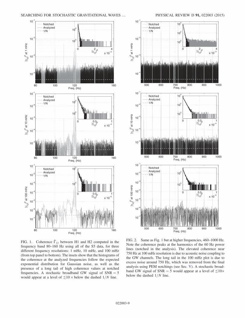
FIG. 1. Coherence Γ̂12 between H1 and H2 computed in thefrequency band 80–160 Hz using all of the S5 data, for threedifferent frequency resolutions: 1 mHz, 10 mHz, and 100 mHz(from top panel to bottom). The insets show that the histograms ofthe coherence at the analyzed frequencies follow the expectedexponential distribution for Gaussian noise, as well as thepresence of a long tail of high coherence values at notchedfrequencies. A stochastic broadband GW signal of SNR ¼ 5would appear at a level of ≲10 × below the dashed 1=N line.

500 600 700 800 900 1000

10−4

10−3

10−2

10−1

Freq. (Hz)

| γ12

|2 at 1

mH

z

NotchedAnalyzed1/N

0 2 4

x 10−3

100

102

104

|γ12

|2

500 600 700 800 900 1000

10−5

10−4

10−3

10−2

10−1

Freq. (Hz)

|γ12

|2 at 1

0 m

Hz

NotchedAnalyzed1/N

0 0.5 1

x 10−4

100

102

104

|γ12

|2

500 600 700 800 900 1000

10−7

10−6

10−5

10−4

10−3

10−2

10−1

Freq. (Hz)

|γ12

|2 at 1

00 m

Hz

NotchedAnalyzed1/N

0 0.5 1

x 10−5

100

102

|γ12

|2

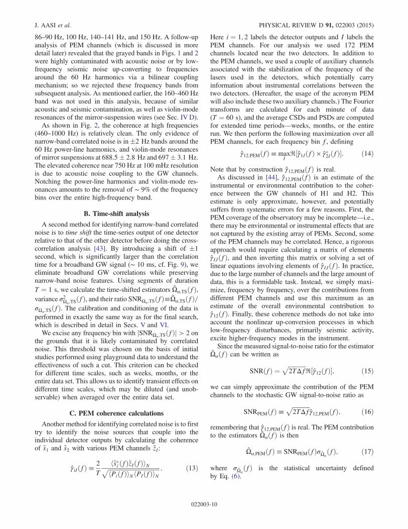
FIG. 2. Same as Fig. 1 but at higher frequencies, 460–1000 Hz.Note the coherence peaks at the harmonics of the 60 Hz powerlines (notched in the analysis). The elevated coherence near750 Hz at 100 mHz resolution is due to acoustic noise coupling tothe GW channels. The long tail in the 100 mHz plot is due toexcess noise around 750 Hz, which was removed from the finalanalysis using PEM notchings (see Sec. V). A stochastic broad-band GW signal of SNR ¼ 5 would appear at a level of ≲10×below the dashed 1=N line.

SEARCHING FOR STOCHASTIC GRAVITATIONAL WAVES … PHYSICAL REVIEW D 91, 022003 (2015)

022003-9

86–90 Hz, 100 Hz, 140–141 Hz, and 150 Hz. A follow-upanalysis of PEM channels (which is discussed in moredetail later) revealed that the grayed bands in Figs. 1 and 2were highly contaminated with acoustic noise or by low-frequency seismic noise up-converting to frequenciesaround the 60 Hz harmonics via a bilinear couplingmechanism; so we rejected these frequency bands fromsubsequent analysis. As mentioned earlier, the 160–460 Hzband was not used in this analysis, because of similaracoustic and seismic contamination, as well as violin-moderesonances of the mirror-suspension wires (see Sec. IV D).As shown in Fig. 2, the coherence at high frequencies

(460–1000 Hz) is relatively clean. The only evidence ofnarrow-band correlated noise is in�2 Hz bands around the60 Hz power-line harmonics, and violin-mode resonancesof mirror suspensions at 688.5� 2.8 Hz and 697� 3.1 Hz.The elevated coherence near 750 Hz at 100 mHz resolutionis due to acoustic noise coupling to the GW channels.Notching the power-line harmonics and violin-mode res-onances amounts to the removal of ∼ 9% of the frequencybins over the entire high-frequency band.

B. Time-shift analysis

A second method for identifying narrow-band correlatednoise is to time shift the time-series output of one detectorrelative to that of the other detector before doing the cross-correlation analysis [43]. By introducing a shift of �1second, which is significantly larger than the correlationtime for a broadband GW signal (∼ 10 ms, cf. Fig. 9), weeliminate broadband GW correlations while preservingnarrow-band noise features. Using segments of durationT ¼ 1 s, we calculate the time-shifted estimators Ω̂α;TSðfÞ,variance σ2Ωα;TS

ðfÞ, and their ratio SNRΩα;TSðfÞ≡Ω̂α;TSðfÞ=σΩα;TSðfÞ. The calibration and conditioning of the data isperformed in exactly the same way as for the final search,which is described in detail in Secs. V and VI.We excise any frequency bin with jSNRΩα;TSðfÞj > 2 on

the grounds that it is likely contaminated by correlatednoise. This threshold was chosen on the basis of initialstudies performed using playground data to understand theeffectiveness of such a cut. This criterion can be checkedfor different time scales, such as weeks, months, or theentire data set. This allows us to identify transient effects ondifferent time scales, which may be diluted (and unob-servable) when averaged over the entire data set.

C. PEM coherence calculations

Another method for identifying correlated noise is to firsttry to identify the noise sources that couple into theindividual detector outputs by calculating the coherenceof ~s1 and ~s2 with various PEM channels ~zI:

γ̂iIðfÞ≡ 2

Th~s�i ðfÞ~zIðfÞiNffiffiffiffiffiffiffiffiffiffiffiffiffiffiffiffiffiffiffiffiffiffiffiffiffiffiffiffiffiffiffiffiffiffiffihPiðfÞiNhPIðfÞiN

p : ð13Þ

Here i ¼ 1; 2 labels the detector outputs and I labels thePEM channels. For our analysis we used 172 PEMchannels located near the two detectors. In addition tothe PEM channels, we used a couple of auxiliary channelsassociated with the stabilization of the frequency of thelasers used in the detectors, which potentially carryinformation about instrumental correlations between thetwo detectors. (Hereafter, the usage of the acronym PEMwill also include these two auxiliary channels.) The Fouriertransforms are calculated for each minute of data(T ¼ 60 s), and the average CSDs and PSDs are computedfor extended time periods—weeks, months, or the entirerun. We then perform the following maximization over allPEM channels, for each frequency bin f, defining

γ̂12;PEMðfÞ≡maxIℜ½γ̂1IðfÞ × γ̂�2IðfÞ�: ð14Þ

Note that by construction γ̂12;PEMðfÞ is real.As discussed in [44], γ̂12;PEMðfÞ is an estimate of the

instrumental or environmental contribution to the coher-ence between the GW channels of H1 and H2. Thisestimate is only approximate, however, and potentiallysuffers from systematic errors for a few reasons. First, thePEM coverage of the observatory may be incomplete—i.e.,there may be environmental or instrumental effects that arenot captured by the existing array of PEMs. Second, someof the PEM channels may be correlated. Hence, a rigorousapproach would require calculating a matrix of elementsγ̂IJðfÞ, and then inverting this matrix or solving a set oflinear equations involving elements of γ̂IJðfÞ. In practice,due to the large number of channels and the large amount ofdata, this is a formidable task. Instead, we simply maxi-mize, frequency by frequency, over the contributions fromdifferent PEM channels and use this maximum as anestimate of the overall environmental contribution toγ̂12ðfÞ. Finally, these coherence methods do not take intoaccount the nonlinear up-conversion processes in whichlow-frequency disturbances, primarily seismic activity,excite higher-frequency modes in the instrument.Since the measured signal-to-noise ratio for the estimator

Ω̂αðfÞ can be written as

SNRðfÞ ¼ffiffiffiffiffiffiffiffiffiffiffiffi2TΔf

pℜ½γ̂12ðfÞ�; ð15Þ

we can simply approximate the contribution of the PEMchannels to the stochastic GW signal-to-noise ratio as

SNRPEMðfÞ≡ffiffiffiffiffiffiffiffiffiffiffiffi2TΔf

pγ̂12;PEMðfÞ; ð16Þ

remembering that γ̂12;PEMðfÞ is real. The PEM contributionto the estimators Ω̂αðfÞ is then

Ω̂α;PEMðfÞ≡ SNRPEMðfÞσΩ̂αðfÞ; ð17Þ

where σΩ̂αðfÞ is the statistical uncertainty defined

by Eq. (6).

J. AASI et al. PHYSICAL REVIEW D 91, 022003 (2015)

022003-10

We can use the PEM coherence calculations in twocomplementary ways. First, we can identify frequency binswith particularly large instrumental or environmental con-tributions by placing a threshold on jSNRPEMðfÞj andexclude them from the analysis. Second, the frequency binsthat pass this data-quality cut may still contain someresidual environmental contamination. We can estimateat least part of this residual contamination by usingΩ̂α;PEMðfÞ for the remaining frequency bins.As part of the analysis procedure, we were able to identify

the PEM channels that were responsible for the largestcoherent noise between the GW channels in H1 and H2 foreach frequency bin. For both the low- and high-frequencyanalyses, microphones and accelerometers in the centralbuilding near the beam splitters of each interferometerregistered the most significant noise. Within approximately1 Hz of the 60 Hz harmonics, magnetometers and voltageline monitors registered the largest correlated noise, but thesefrequencies were already removed from the analysis due tothe significant coherence (noise) level at these frequencies,as mentioned in Sec. IVA.

D. Comparing PEM-coherence and time-shift methods

Figure 3 shows a comparison of the SNRs calculated bythe PEM-coherence and time-shift methods. The agreementbetween these two very different techniques in identifying

contaminated frequency bins (those with jSNRj≳ a few) isremarkably good, which is an indication of their robustnessand effectiveness. Moreover, Fig. 3 shows that the fre-quency region between 200 Hz and 460 Hz is particularlycontaminated by environmental and/or instrumental effects.Hence, in this analysis we focus on the low-frequencyregion (80–160 Hz) which is the most sensitive to cosmo-logical backgrounds (i.e., spectral index α ¼ 0), and on thehigh-frequency region (460–1000 Hz) which is less con-taminated and more suitable for searches for astrophysi-cally generated backgrounds (e.g., α ¼ 3).We emphasize that the PEM channels only monitor the

instrument and the environment, and are not sensitive toGWs. Similarly, the time-shift analysis, with a time shift of�1 second, is insensitive to broadband GW signals. Hence,any data-quality cuts based on the PEM and time-shiftstudies will not affect the astrophysical signatures in thedata—i.e., they do not bias our estimates of the amplitudeof a SGWB.

E. Other potential nonastrophysicalsources of correlation

We note that any correlations that are produced byenvironmental signals that are not detected by the PEMsensors will not be detected by the PEM-coherencetechnique. Furthermore, if such correlations, or correlationsfrom a nonenvironmental source, are broadband and flat(i.e., do not vary with frequency over our band), they willnot be detected by either the PEM-coherence or the time-shift method. One potential source of broadband correlationbetween the two GW channels is the data acquisitionsystem itself. We investigated this possibility by looking forcorrelations between 153 channel pairs that had no physicalreason to be correlated. We found no broadband correla-tions, although we did find an unexplained narrow-bandcorrelation at 281.5 Hz between 10 of 153 channel pairs.Note that 281.5 Hz is outside of the frequency bandsanalyzed in this study.We addressed the potential of correlations from unmo-

nitored environmental signals by searching for couplingsites four times over the course of the run by injecting largebut localized acoustic, seismic, magnetic, and RF signals.New sensors were installed at the two coupling sites thathad the least coverage. However, we found that the newsensors, even after scaling up to the full analysis period,contribute less than 1% of the total frequency notches;hence it is safe to assume that we had sufficient PEMcoverage throughout our analysis period.We also examined the possibility of correlations between

the H1 and H2 detectors being generated by scattered light.We considered two mechanisms: first, light scattered fromone detector affecting the other detector, and second, lightfrom both detectors scattering off of the same site andreturning to the originating detectors. We did not observe,and do not expect to observe, the first mechanism because

200 400 600 800 100010

−2

10−1

100

101

102

103

104

|SN

R|

Freq. (Hz)

SNRPEM

SNRTS

FIG. 3 (color online). Comparison of the (absolute value of the)SNRs calculated by the PEM-coherence and time-shift tech-niques. The vertical dotted lines indicate the frequency bandsused for the low- (80–160 Hz; black dotted lines) and high-frequency (460–1000 Hz; magenta dotted lines) analyses. Notethat SNRΩα;TSðfÞ is a true signal-to-noise ratio, so values ≲2 aredominated by random statistical fluctuations. SNRΩα ;PEMðfÞ, onthe other hand, is an estimate of the PEM contribution to thesignal-to-noise ratio, so values even much lower than 2 aremeaningful measurements (i.e., they are not statistical fluctua-tions). The two methods agree very well in identifying contami-nated frequency bins or bands. Note that both methods indicatethat the 80–160 Hz and 460–1000 Hz bands have relatively lowlevels of contamination.

SEARCHING FOR STOCHASTIC GRAVITATIONAL WAVES … PHYSICAL REVIEW D 91, 022003 (2015)

022003-11

the frequencies of the two lasers, while very stable, maydiffer by gigahertz. If light from one interferometer scattersinto the main beam of the other, it will likely be at a verydifferent frequency and will not produce signals in our8 kHz band when it beats against the reference light for thatinterferometer.Nevertheless, we checked for a correlation produced by

light from one detector entering the other by looking for thecalibration signals [5] injected into one detector in thesignal of the second detector. During S5, the followingcalibration line frequencies were injected into H1 and H2:46.70 Hz, 393.10 Hz, 1144.30 Hz (H1) and 54.10 Hz,407.30 Hz, 1159.7 Hz (H2). We note here that all thosefrequencies are outside of our analysis bands. We observedno correlation beyond the statistical error of the measure-ment at any of the three calibration line frequencies foreither of the two detectors. This check was done for everyweek and month and for the entire S5 data set. Hence, weconclude that potential signals carried by the light in onedetector are not coupled into the other detector.In contrast, we have observed the second scattering

mechanism, in which scattered light from the H1 beamreturns to the H1 main beam and H2 light returns to the H2main beam. This type of scattering can produce H1-H2coupling if scattered light from H1 and from H2 both reflectoff of the same vibrating surface (which modulates thelength of the scattering paths) before recombining with theiroriginal main beams. This mechanism is thought to accountfor the observation that shaking the reflective end cap of the4 km beam tube (just beyond an H1 end test mass) produceda shaking-frequency peak in both H1 and H2 GW channels,even though the nearest H2 component was 2 km away.However, this scattering mechanism is covered by the PEMsystem since the vibrations that modulate the beam pathoriginate in the monitored environment.We tested our expectation that scattering-induced corre-

lations would be identified by our PEM-coherence method.We initiated a program to identify the most importantscattering sites by mounting shakers on the vacuum systemat 21 different locations that were selected as potentialscattering sites, and searching for the shaking signal in theGW channels. All significant scattering sites that we foundin this way were well monitored by the PEM system. At thesite that produced the greatest coherence between the twodetectors (a reflective flange close to and perpendicular tothe beam paths of both interferometers), we mounted anaccelerometer and found that the coherence between thisaccelerometer and the two GW channels was no greater thanthat for the sensors in the preexisting sensor system. Theseresults suggest that the PEM system adequately monitoredscattering coupling. As we shall show in Sec. VI A below, nocorrelated noise (either environmental or instrumental, eithernarrow band or broadband) that is not adequately covered bythe PEM system is identified in the high-frequency analysis,further solidifying the adequacy of PEM system.

V. ANALYSIS PROCEDURE

In the previous section we described a number ofmethods for identifying correlated noise when searchingfor a SGWB. Here we enumerate the steps for selecting thetime segments and frequency bands that were subsequentlyused for the analysis.Step 1: We begin by selecting time periods that pass a

number of data-quality flags. In particular, we rejectperiods when (i) there are problems with the calibrationof the data; (ii) the interferometers are within 30 s of loss ofservo control; (iii) there are artificial signals inserted intothe data for calibration and characterization purposes;(iv) there are PEM noise injections; (v) various dataacquisition overflows are observed; or (vi) there is missingdata. With these cuts, the intersection of the H1 and H2analyzable time was ∼ 462 days for the S5 run.Step 2: After selecting suitable data segments, we make a

first pass at determining the frequency bins to use in theanalysis by calculating the overall coherence between thedetector outputs as described in Sec. IVA. Excess coher-ence levels led us to reject the frequencies 86–90 Hz,100 Hz, 102–126 Hz, 140.25–141.25 Hz, and 150 Hz in thelow-frequency band (80–160 Hz), as well as�2 Hz aroundthe 60 Hz power-line harmonics and the violin-moderesonances at 688.5� 2.8 Hz and 697� 3.1 Hz in thehigh-frequency band (460–1000 Hz). It also identified aperiod of about 17 days in June 2007 (between GPS times866526322 and 867670285), during which the detector H2suffered from excessive transient noise glitches. We rejectthat period from the analysis.Step 3: We perform a search for transient excess power in

the data using the wavelet-based Kleine Welle algorithm[45], which was originally designed for detecting GWbursts. This algorithm is applied to the output of bothdetectors, producing a list of triggers for each detector. Wethen search the two trigger lists and reject any segment thatcontains transients with a Kleine Welle significance largerthan 50 in either of the two detectors. The value of 50 is aconservative threshold, chosen based on other studies doneon the distribution of such triggers in S5 [32].Step 4: Having determined the reasonably good fre-

quency bands, we then calculate Ω̂α and its uncertainty σΩ̂α

summed over the whole band, cf. Eq. (7). The purpose ofthis calculation is to perform another level of data qualityselection in the time domain by identifying noisy segmentsof 60 s duration. It is similar to the nonstationarity cut usedin the previous analyses [26–28,46] where we remove timesegments whose σΩ̂α

differs, by a predetermined amount,from that calculated by averaging over two neighboringsegments. Here we use a 20% threshold on the difference.The combination of the time-domain data quality cutsdescribed in Steps 1–4 removed about 22% of the availableS5 H1-H2 data.Step 5: After identifying and rejecting noisy time seg-

ments and frequency bins using Steps 1–4, we then use the

J. AASI et al. PHYSICAL REVIEW D 91, 022003 (2015)

022003-12

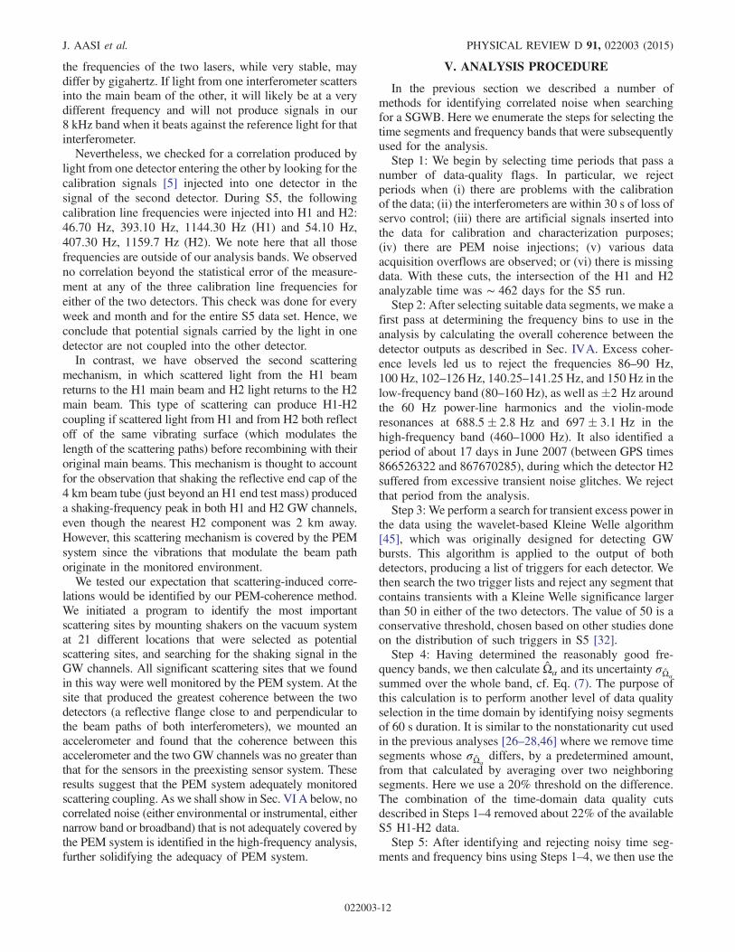
time-shift and PEM-coherence methods described inSecs. IV B and IV C to identify any remaining contami-nated frequency bins. To remove bad frequency bins, wesplit the S5 data set into weeklong periods and for eachweek, we reject any frequency bin for which eitherjSNRΩα;TSðfÞj or jSNRΩα;PEMðfÞj exceeds a predeterminedthreshold in the given week, the corresponding month, or inthe entire S5 data set. This procedure generates (different)sets of frequency notchings for each week of the S5 dataset. In the analysis we use two different sets of SNRthreshold values for the cut, which are further describedin Sec. VI.Figure 4 is a spectrogram of SNRΩ0;PEM for the 80–

160 Hz band for all weeks in S5; the visible structurerepresents correlated noise between H1 and H2, which wasidentified and subsequently excluded from the analysis bythe H1-H2 coherence, time-shift, and PEM-coherencemeasurements.Note that previous stochastic analyses using LIGO data

[26–28,46] followed only Steps 1, 2, and 4. Steps 3 and 5were developed for this particular analysis.Having defined the time segments and frequency bins to

be rejected in each week of the S5 data, we proceed with thecalculation of the estimators and standard errors, Ω̂αðfÞ andσΩ̂α

ðfÞ, in much the same manner as in previous searchesfor isotropic stochastic backgrounds [26–28,47]. The datais divided into T ¼ 60 s segments, decimated to 1024 Hzfor the low-frequency analysis and 4096 Hz for the high-frequency analysis, and high-pass filtered with a sixth orderButterworth filter with 32 Hz knee frequency. Each analysissegment is Hann windowed, and to recover the loss ofsignal-to-noise ratio due to Hann windowing, segments are50% overlapped. Estimators and standard errors for eachsegment are evaluated with a Δf ¼ 0.25 Hz frequency

resolution, using the frequency mask of the week to whichthe segment belongs. Aweighted average is performed overall segments and all frequency bins, with inverse variances,as in Eq. (7), but properly accounting for overlapping.

VI. ANALYSIS RESULTS

The analysis is separated into two parts corresponding tosearches for SGWBs with spectral index α ¼ 0 and α ¼ 3as described in Sec. III. Since the strain output of aninterferometer due to GWs is SgwðfÞ ∝ fα−3 (see Eq. (3),the case α ¼ 0 is dominated by low frequencies whileα ¼ 3 is independent of frequency. Since for α ¼ 3 there isno preferred frequency band, and since previous analyses[46] for stochastic backgrounds with α ¼ 3 considered onlyhigh frequencies, we also used only high frequencies forthe α ¼ 3 case. Thus, the two cases of α ¼ 0 and α ¼ 3correspond to the analysis of the low- and high-frequencybands, respectively. In this section, we present the results ofthe analyses in the two different frequency bands asdefined in Sec. IV D corresponding to the two differentvalues of α.To illustrate the effect of the various noise removal

methods described in the previous two sections, we give theresults as different stages of cuts are applied to the data (seeTable I). The threshold value used at stage III comes froman initial study performed using playground data to under-stand the effectiveness of the PEM-coherence method infinding problematic frequency bins in the H1-H2 analysis,and hence those results are considered as blind analysisresults. But a post-unblinding study showed that we couldlower the SNRPEM threshold to values as low as 0.5 (for lowfrequency) and 1 (for high frequency), which are used atstage IV. These postblinding results are used in the final

Week in S5

Fre

quen

cy (

Hz)

20 40 60 80 10080

90

100

110

120

130

140

150

160

|SN

R|

0

0.5

1

1.5

2

Week in S5

Fre

quen

cy (

Hz)

20 40 60 80 100

500

550

600

650

700

750

800

850

900

950

1000

|SN

R|

0

0.5

1

1.5

2

FIG. 4 (color online). Spectrograms displaying the absolute value of SNRΩ;PEMðfÞ for 80–160 Hz (left panel) and 460–1000 Hz (rightpanel) as a function of the week in S5. The horizontal dark (blue) bands correspond to initial frequency notches as described in Step 2(Sec. V) and vertical dark (blue) lines correspond to unavailability of data due to detector downtime. The large SNR structures seen inthe plots were removed from the low- and high-frequency analyses.

SEARCHING FOR STOCHASTIC GRAVITATIONAL WAVES … PHYSICAL REVIEW D 91, 022003 (2015)

022003-13

upper-limit calculations. For threshold values < 0.5 (lowfrequency) or < 1 (high frequency), the PEM-coherencecontribution, Ω̂α;PEM, varies randomly as the threshold ischanged indicating the statistical noise limit of the PEM-coherence method.

A. High-frequency results

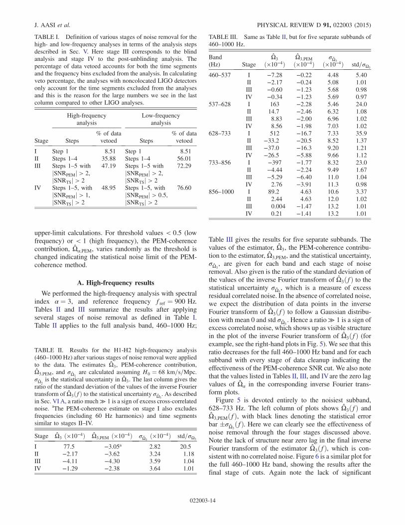
We performed the high-frequency analysis with spectralindex α ¼ 3, and reference frequency fref ¼ 900 Hz.Tables II and III summarize the results after applyingseveral stages of noise removal as defined in Table I.Table II applies to the full analysis band, 460–1000 Hz;

Table III gives the results for five separate subbands. Thevalues of the estimator, Ω̂3, the PEM-coherence contribu-tion to the estimator, Ω̂3;PEM, and the statistical uncertainty,σΩ̂3

, are given for each band and each stage of noiseremoval. Also given is the ratio of the standard deviation ofthe values of the inverse Fourier transform of Ω̂3ðfÞ to thestatistical uncertainty σΩ̂3

, which is a measure of excessresidual correlated noise. In the absence of correlated noise,we expect the distribution of data points in the inverseFourier transform of Ω̂3ðfÞ to follow a Gaussian distribu-tion with mean 0 and std σΩ̂3

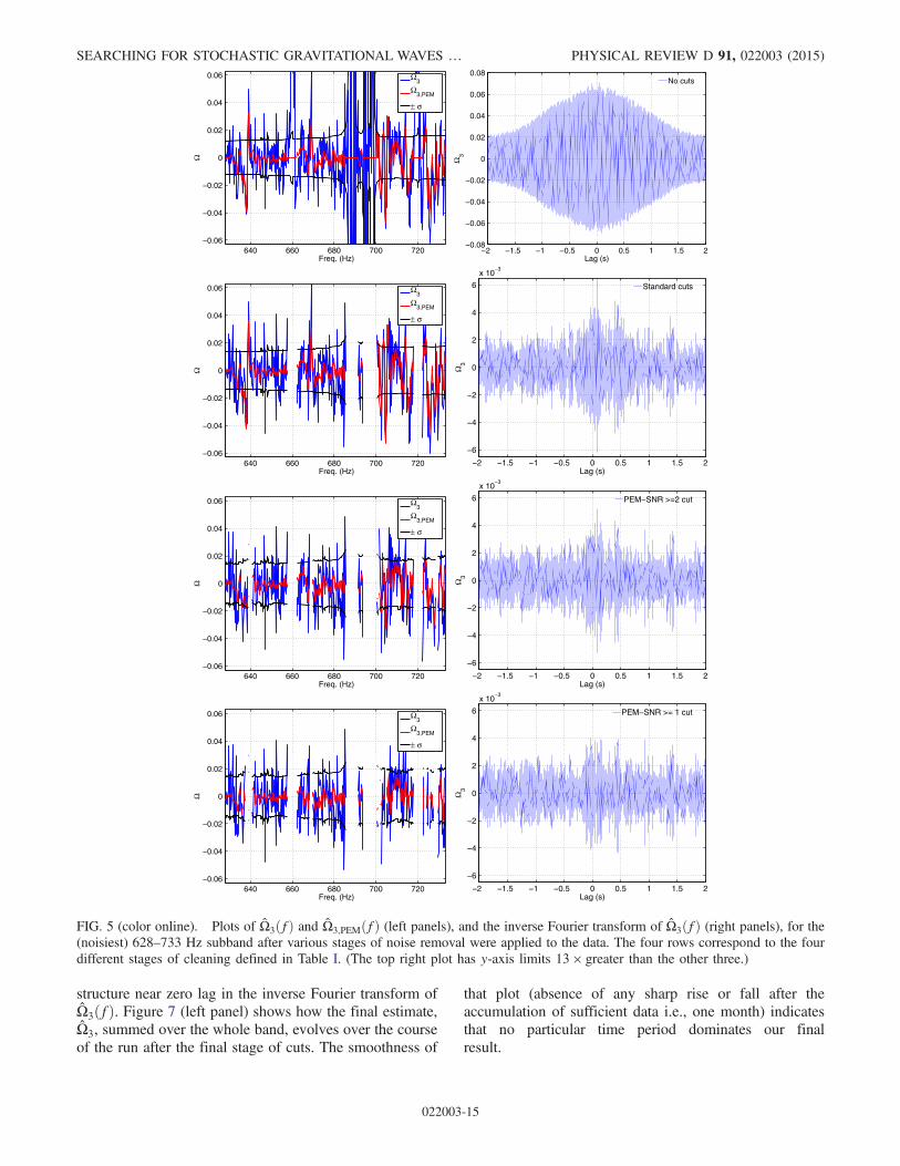
. Hence a ratio≫ 1 is a sign ofexcess correlated noise, which shows up as visible structurein the plot of the inverse Fourier transform of Ω̂3ðfÞ (forexample, see the right-hand plots in Fig. 5). We see that thisratio decreases for the full 460–1000 Hz band and for eachsubband with every stage of data cleanup indicating theeffectiveness of the PEM-coherence SNR cut. We also notethat the values listed in Tables II, III, and IVare the zero lagvalues of Ω̂α in the corresponding inverse Fourier trans-form plots.Figure 5 is devoted entirely to the noisiest subband,

628–733 Hz. The left column of plots shows Ω̂3ðfÞ andΩ̂3;PEMðfÞ, with black lines denoting the statistical errorbar �σΩ̂3

ðfÞ. Here we can clearly see the effectiveness ofnoise removal through the four stages discussed above.Note the lack of structure near zero lag in the final inverseFourier transform of the estimator Ω̂3ðfÞ, which is con-sistent with no correlated noise. Figure 6 is a similar plot forthe full 460–1000 Hz band, showing the results after thefinal stage of cuts. Again note the lack of significant

TABLE I. Definition of various stages of noise removal for thehigh- and low-frequency analyses in terms of the analysis stepsdescribed in Sec. V. Here stage III corresponds to the blindanalysis and stage IV to the post-unblinding analysis. Thepercentage of data vetoed accounts for both the time segmentsand the frequency bins excluded from the analysis. In calculatingveto percentage, the analyses with noncolocated LIGO detectorsonly account for the time segments excluded from the analysesand this is the reason for the large numbers we see in the lastcolumn compared to other LIGO analyses.

High-frequencyanalysis

Low-frequencyanalysis

Stage Steps% of datavetoed Steps

% of datavetoed

I Step 1 8.51 Step 1 8.51II Steps 1–4 35.88 Steps 1–4 56.01III Steps 1–5 with 47.19 Steps 1–5 with 72.29

jSNRPEMj > 2, jSNRPEMj > 2,jSNRTSj > 2 jSNRTSj > 2

IV Steps 1–5, with 48.95 Steps 1–5, with 76.60jSNRPEMj > 1, jSNRPEMj > 0.5,jSNRTSj > 2 jSNRTSj > 2

TABLE II. Results for the H1-H2 high-frequency analysis(460–1000 Hz) after various stages of noise removal were appliedto the data. The estimates Ω̂3, PEM-coherence contribution,Ω̂3;PEM, and σΩ̂3

are calculated assuming H0 ¼ 68 km=s=Mpc.σΩ̂3

is the statistical uncertainty in Ω̂3. The last column gives theratio of the standard deviation of the values of the inverse Fouriertransform of Ω̂3ðfÞ to the statistical uncertainty σΩ̂3

. As describedin Sec. VI A, a ratio much≫ 1 is a sign of excess cross-correlatednoise. aThe PEM-coherence estimate on stage I also excludesfrequencies (including 60 Hz harmonics) and time segmentssimilar to stages II–IV.

Stage Ω̂3 ð×10−4Þ Ω̂3;PEM ð×10−4Þ σΩ̂3ð×10−4Þ std=σΩ3

I 77.5 −3.05a 2.82 20.5II −2.17 −3.62 3.24 1.18III −4.11 −4.30 3.59 1.04IV −1.29 −2.38 3.64 1.01

TABLE III. Same as Table II, but for five separate subbands of460–1000 Hz.

Band(Hz) Stage

Ω̂3

ð×10−4ÞΩ̂3;PEMð×10−4Þ

σΩ̂3ð×10−4Þ std=σΩ3

460–537 I −7.28 −0.22 4.48 5.40II −2.17 −0.24 5.08 1.01III −0.60 −1.23 5.68 0.98IV −0.34 −1.23 5.69 0.97

537–628 I 163 −2.28 5.46 24.0II 14.7 −2.46 6.32 1.08III 8.83 −2.00 6.96 1.02IV 8.56 −1.98 7.03 1.02

628–733 I 512 −16.7 7.33 35.9II −33.2 −20.5 8.52 1.37III −37.0 −16.3 9.20 1.21IV −26.5 −5.88 9.66 1.12

733–856 I −397 −1.77 8.32 23.0II −4.44 −2.24 9.49 1.67III −5.29 −6.40 11.0 1.04IV 2.76 −3.91 11.3 0.98

856–1000 I 89.2 4.63 10.6 3.37II 2.44 4.63 12.0 1.02III 0.004 −1.47 13.2 1.01IV 0.21 −1.41 13.2 1.01

J. AASI et al. PHYSICAL REVIEW D 91, 022003 (2015)

022003-14

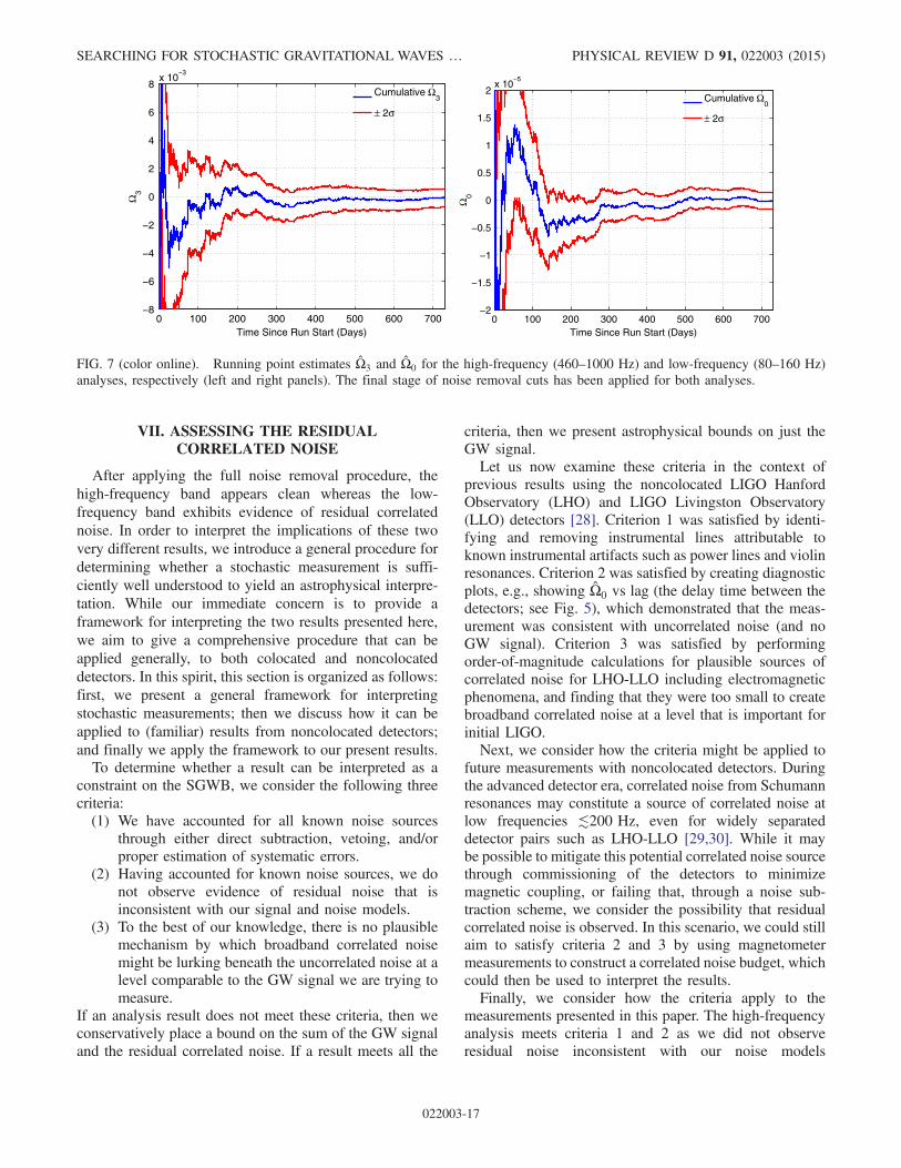
structure near zero lag in the inverse Fourier transform ofΩ̂3ðfÞ. Figure 7 (left panel) shows how the final estimate,Ω̂3, summed over the whole band, evolves over the courseof the run after the final stage of cuts. The smoothness of

that plot (absence of any sharp rise or fall after theaccumulation of sufficient data i.e., one month) indicatesthat no particular time period dominates our finalresult.

640 660 680 700 720−0.06

−0.04

−0.02

0

0.02

0.04

0.06

Ω

Freq. (Hz)

Ω3

Ω3,PEM

± σ

−2 −1.5 −1 −0.5 0 0.5 1 1.5 2−0.08

−0.06

−0.04

−0.02

0

0.02

0.04

0.06

0.08

Ω3

Lag (s)

No cuts

640 660 680 700 720−0.06

−0.04

−0.02

0

0.02

0.04

0.06

Ω

Freq. (Hz)

Ω3

Ω3,PEM

± σ

−2 −1.5 −1 −0.5 0 0.5 1 1.5 2

−6

−4

−2

0

2

4

6

x 10−3

Ω3

Lag (s)

Standard cuts

640 660 680 700 720−0.06

−0.04

−0.02

0

0.02

0.04

0.06

Ω

Freq. (Hz)

Ω3

Ω3,PEM

± σ

−2 −1.5 −1 −0.5 0 0.5 1 1.5 2

−6

−4

−2

0

2

4

6

x 10−3

Ω3

Lag (s)

PEM−SNR >=2 cut

640 660 680 700 720−0.06

−0.04

−0.02

0

0.02

0.04

0.06

Ω

Freq. (Hz)

Ω3

Ω3,PEM

± σ

−2 −1.5 −1 −0.5 0 0.5 1 1.5 2

−6

−4

−2

0

2

4

6

x 10−3

Ω3

Lag (s)

PEM−SNR >= 1 cut

FIG. 5 (color online). Plots of Ω̂3ðfÞ and Ω̂3;PEMðfÞ (left panels), and the inverse Fourier transform of Ω̂3ðfÞ (right panels), for the(noisiest) 628–733 Hz subband after various stages of noise removal were applied to the data. The four rows correspond to the fourdifferent stages of cleaning defined in Table I. (The top right plot has y-axis limits 13 × greater than the other three.)

SEARCHING FOR STOCHASTIC GRAVITATIONAL WAVES … PHYSICAL REVIEW D 91, 022003 (2015)

022003-15

B. Low-frequency results

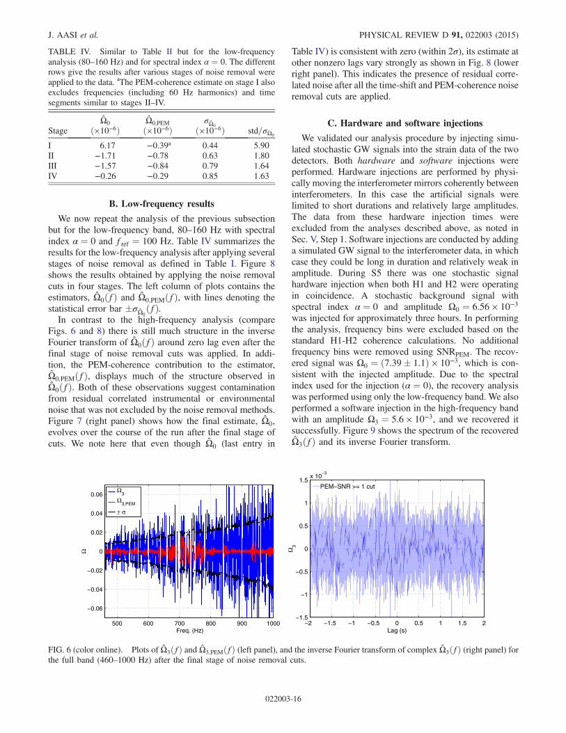
We now repeat the analysis of the previous subsectionbut for the low-frequency band, 80–160 Hz with spectralindex α ¼ 0 and fref ¼ 100 Hz. Table IV summarizes theresults for the low-frequency analysis after applying severalstages of noise removal as defined in Table I. Figure 8shows the results obtained by applying the noise removalcuts in four stages. The left column of plots contains theestimators, Ω̂0ðfÞ and Ω̂0;PEMðfÞ, with lines denoting thestatistical error bar �σΩ̂0

ðfÞ.In contrast to the high-frequency analysis (compare

Figs. 6 and 8) there is still much structure in the inverseFourier transform of Ω̂0ðfÞ around zero lag even after thefinal stage of noise removal cuts was applied. In addi-tion, the PEM-coherence contribution to the estimator,Ω̂0;PEMðfÞ, displays much of the structure observed inΩ̂0ðfÞ. Both of these observations suggest contaminationfrom residual correlated instrumental or environmentalnoise that was not excluded by the noise removal methods.Figure 7 (right panel) shows how the final estimate, Ω̂0,evolves over the course of the run after the final stage ofcuts. We note here that even though Ω̂0 (last entry in

Table IV) is consistent with zero (within 2σ), its estimate atother nonzero lags vary strongly as shown in Fig. 8 (lowerright panel). This indicates the presence of residual corre-lated noise after all the time-shift and PEM-coherence noiseremoval cuts are applied.

C. Hardware and software injections

We validated our analysis procedure by injecting simu-lated stochastic GW signals into the strain data of the twodetectors. Both hardware and software injections wereperformed. Hardware injections are performed by physi-cally moving the interferometer mirrors coherently betweeninterferometers. In this case the artificial signals werelimited to short durations and relatively large amplitudes.The data from these hardware injection times wereexcluded from the analyses described above, as noted inSec. V, Step 1. Software injections are conducted by addinga simulated GW signal to the interferometer data, in whichcase they could be long in duration and relatively weak inamplitude. During S5 there was one stochastic signalhardware injection when both H1 and H2 were operatingin coincidence. A stochastic background signal withspectral index α ¼ 0 and amplitude Ω0 ¼ 6.56 × 10−3

was injected for approximately three hours. In performingthe analysis, frequency bins were excluded based on thestandard H1-H2 coherence calculations. No additionalfrequency bins were removed using SNRPEM. The recov-ered signal was Ω0 ¼ ð7.39� 1.1Þ × 10−3, which is con-sistent with the injected amplitude. Due to the spectralindex used for the injection (α ¼ 0), the recovery analysiswas performed using only the low-frequency band. We alsoperformed a software injection in the high-frequency bandwith an amplitude Ω3 ¼ 5.6 × 10−3, and we recovered itsuccessfully. Figure 9 shows the spectrum of the recoveredΩ̂3ðfÞ and its inverse Fourier transform.

TABLE IV. Similar to Table II but for the low-frequencyanalysis (80–160 Hz) and for spectral index α ¼ 0. The differentrows give the results after various stages of noise removal wereapplied to the data. aThe PEM-coherence estimate on stage I alsoexcludes frequencies (including 60 Hz harmonics) and timesegments similar to stages II–IV.

StageΩ̂0

ð×10−6ÞΩ̂0;PEMð×10−6Þ

σΩ̂0ð×10−6Þ std=σΩ0

I 6.17 −0.39a 0.44 5.90II −1.71 −0.78 0.63 1.80III −1.57 −0.84 0.79 1.64IV −0.26 −0.29 0.85 1.63

500 600 700 800 900 1000

−0.06

−0.04

−0.02

0

0.02

0.04

0.06

Ω

Freq. (Hz)

Ω3

Ω3,PEM

± σ

−2 −1.5 −1 −0.5 0 0.5 1 1.5 2−1.5

−1

−0.5

0

0.5

1

1.5x 10

−3

Ω3

Lag (s)

PEM−SNR >= 1 cut

FIG. 6 (color online). Plots of Ω̂3ðfÞ and Ω̂3;PEMðfÞ (left panel), and the inverse Fourier transform of complex Ω̂3ðfÞ (right panel) forthe full band (460–1000 Hz) after the final stage of noise removal cuts.

J. AASI et al. PHYSICAL REVIEW D 91, 022003 (2015)

022003-16

VII. ASSESSING THE RESIDUALCORRELATED NOISE

After applying the full noise removal procedure, thehigh-frequency band appears clean whereas the low-frequency band exhibits evidence of residual correlatednoise. In order to interpret the implications of these twovery different results, we introduce a general procedure fordetermining whether a stochastic measurement is suffi-ciently well understood to yield an astrophysical interpre-tation. While our immediate concern is to provide aframework for interpreting the two results presented here,we aim to give a comprehensive procedure that can beapplied generally, to both colocated and noncolocateddetectors. In this spirit, this section is organized as follows:first, we present a general framework for interpretingstochastic measurements; then we discuss how it can beapplied to (familiar) results from noncolocated detectors;and finally we apply the framework to our present results.To determine whether a result can be interpreted as a

constraint on the SGWB, we consider the following threecriteria:(1) We have accounted for all known noise sources

through either direct subtraction, vetoing, and/orproper estimation of systematic errors.

(2) Having accounted for known noise sources, we donot observe evidence of residual noise that isinconsistent with our signal and noise models.

(3) To the best of our knowledge, there is no plausiblemechanism by which broadband correlated noisemight be lurking beneath the uncorrelated noise at alevel comparable to the GW signal we are trying tomeasure.

If an analysis result does not meet these criteria, then weconservatively place a bound on the sum of the GW signaland the residual correlated noise. If a result meets all the

criteria, then we present astrophysical bounds on just theGW signal.Let us now examine these criteria in the context of

previous results using the noncolocated LIGO HanfordObservatory (LHO) and LIGO Livingston Observatory(LLO) detectors [28]. Criterion 1 was satisfied by identi-fying and removing instrumental lines attributable toknown instrumental artifacts such as power lines and violinresonances. Criterion 2 was satisfied by creating diagnosticplots, e.g., showing Ω̂0 vs lag (the delay time between thedetectors; see Fig. 5), which demonstrated that the meas-urement was consistent with uncorrelated noise (and noGW signal). Criterion 3 was satisfied by performingorder-of-magnitude calculations for plausible sources ofcorrelated noise for LHO-LLO including electromagneticphenomena, and finding that they were too small to createbroadband correlated noise at a level that is important forinitial LIGO.Next, we consider how the criteria might be applied to

future measurements with noncolocated detectors. Duringthe advanced detector era, correlated noise from Schumannresonances may constitute a source of correlated noise atlow frequencies ≲200 Hz, even for widely separateddetector pairs such as LHO-LLO [29,30]. While it maybe possible to mitigate this potential correlated noise sourcethrough commissioning of the detectors to minimizemagnetic coupling, or failing that, through a noise sub-traction scheme, we consider the possibility that residualcorrelated noise is observed. In this scenario, we could stillaim to satisfy criteria 2 and 3 by using magnetometermeasurements to construct a correlated noise budget, whichcould then be used to interpret the results.Finally, we consider how the criteria apply to the

measurements presented in this paper. The high-frequencyanalysis meets criteria 1 and 2 as we did not observeresidual noise inconsistent with our noise models

0 100 200 300 400 500 600 700−8

−6

−4

−2

0

2

4

6

8x 10

−3

Ω3

Time Since Run Start (Days)

Cumulative Ω3

± 2σ

0 100 200 300 400 500 600 700−2

−1.5

−1

−0.5

0

0.5

1

1.5

2x 10

−5

Ω0

Time Since Run Start (Days)

Cumulative Ω0

± 2σ

FIG. 7 (color online). Running point estimates Ω̂3 and Ω̂0 for the high-frequency (460–1000 Hz) and low-frequency (80–160 Hz)analyses, respectively (left and right panels). The final stage of noise removal cuts has been applied for both analyses.

SEARCHING FOR STOCHASTIC GRAVITATIONAL WAVES … PHYSICAL REVIEW D 91, 022003 (2015)

022003-17

80 90 100 110 120 130 140 150 160−4

−3

−2

−1

0

1

2

3

4x 10

−5

Ω

Freq. (Hz)

Ω0

Ω0,PEM

± σ

−2 −1.5 −1 −0.5 0 0.5 1 1.5 2−1

−0.8

−0.6

−0.4

−0.2

0

0.2

0.4

0.6

0.8

1x 10

−5

Ω0

Lag (s)

No cuts

80 90 100 110 120 130 140 150 160−4

−3

−2

−1

0

1

2

3

4x 10

−5

Ω

Freq. (Hz)

Ω0

Ω0,PEM

± σ

−2 −1.5 −1 −0.5 0 0.5 1 1.5 2−1

−0.8

−0.6

−0.4

−0.2

0

0.2

0.4

0.6

0.8

1x 10

−5

Ω0

Lag (s)

Standard cuts

80 90 100 110 120 130 140 150 160−4

−3

−2

−1

0

1

2

3

4x 10

−5

Ω

Freq. (Hz)

Ω0

Ω0,PEM

± σ

−2 −1.5 −1 −0.5 0 0.5 1 1.5 2−1

−0.8

−0.6

−0.4

−0.2

0

0.2

0.4

0.6

0.8

1x 10

−5

Ω0

Lag (s)

PEM−SNR >=2 cut

80 90 100 110 120 130 140 150 160−4

−3

−2

−1

0

1

2

3

4x 10

−5

Ω

Freq. (Hz)

Ω0

Ω0,PEM

± σ

−2 −1.5 −1 −0.5 0 0.5 1 1.5 2−1

−0.8

−0.6

−0.4

−0.2

0

0.2

0.4

0.6

0.8

1x 10

−5

Ω0

Lag (s)

PEM−SNR >= 0.5 cut

FIG. 8 (color online). Plots of Ω̂0ðfÞ and Ω̂0;PEMðfÞ (left panels), and the inverse Fourier transform of Ω̂0ðfÞ (right panels) for the80–160 Hz band after various stages of noise removal were applied to the data. The four rows correspond to the four different stages ofcleaning defined in Table I.

J. AASI et al. PHYSICAL REVIEW D 91, 022003 (2015)

022003-18

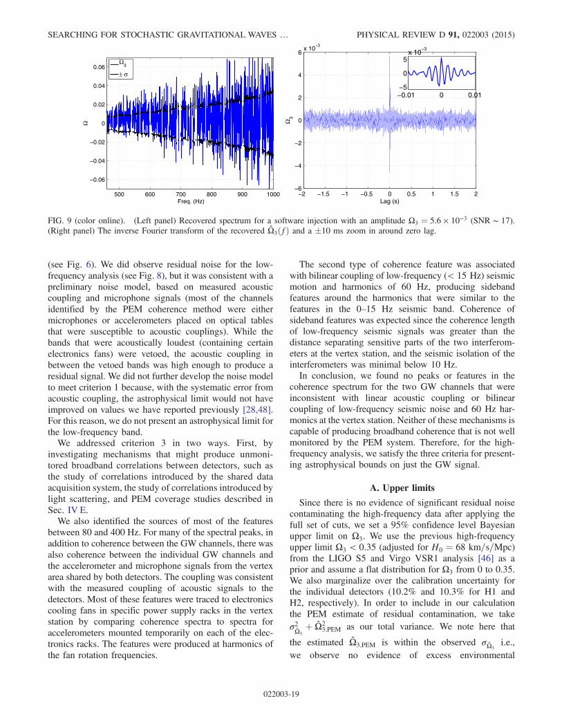
(see Fig. 6). We did observe residual noise for the low-frequency analysis (see Fig. 8), but it was consistent with apreliminary noise model, based on measured acousticcoupling and microphone signals (most of the channelsidentified by the PEM coherence method were eithermicrophones or accelerometers placed on optical tablesthat were susceptible to acoustic couplings). While thebands that were acoustically loudest (containing certainelectronics fans) were vetoed, the acoustic coupling inbetween the vetoed bands was high enough to produce aresidual signal. We did not further develop the noise modelto meet criterion 1 because, with the systematic error fromacoustic coupling, the astrophysical limit would not haveimproved on values we have reported previously [28,48].For this reason, we do not present an astrophysical limit forthe low-frequency band.We addressed criterion 3 in two ways. First, by

investigating mechanisms that might produce unmoni-tored broadband correlations between detectors, such asthe study of correlations introduced by the shared dataacquisition system, the study of correlations introduced bylight scattering, and PEM coverage studies described inSec. IV E.We also identified the sources of most of the features

between 80 and 400 Hz. For many of the spectral peaks, inaddition to coherence between the GW channels, there wasalso coherence between the individual GW channels andthe accelerometer and microphone signals from the vertexarea shared by both detectors. The coupling was consistentwith the measured coupling of acoustic signals to thedetectors. Most of these features were traced to electronicscooling fans in specific power supply racks in the vertexstation by comparing coherence spectra to spectra foraccelerometers mounted temporarily on each of the elec-tronics racks. The features were produced at harmonics ofthe fan rotation frequencies.

The second type of coherence feature was associatedwith bilinear coupling of low-frequency (< 15 Hz) seismicmotion and harmonics of 60 Hz, producing sidebandfeatures around the harmonics that were similar to thefeatures in the 0–15 Hz seismic band. Coherence ofsideband features was expected since the coherence lengthof low-frequency seismic signals was greater than thedistance separating sensitive parts of the two interferom-eters at the vertex station, and the seismic isolation of theinterferometers was minimal below 10 Hz.In conclusion, we found no peaks or features in the

coherence spectrum for the two GW channels that wereinconsistent with linear acoustic coupling or bilinearcoupling of low-frequency seismic noise and 60 Hz har-monics at the vertex station. Neither of these mechanisms iscapable of producing broadband coherence that is not wellmonitored by the PEM system. Therefore, for the high-frequency analysis, we satisfy the three criteria for present-ing astrophysical bounds on just the GW signal.

A. Upper limits

Since there is no evidence of significant residual noisecontaminating the high-frequency data after applying thefull set of cuts, we set a 95% confidence level Bayesianupper limit on Ω3. We use the previous high-frequencyupper limit Ω3 < 0.35 (adjusted for H0 ¼ 68 km=s=Mpc)from the LIGO S5 and Virgo VSR1 analysis [46] as aprior and assume a flat distribution for Ω3 from 0 to 0.35.We also marginalize over the calibration uncertainty forthe individual detectors (10.2% and 10.3% for H1 andH2, respectively). In order to include in our calculationthe PEM estimate of residual contamination, we takeσ2Ω̂3

þ Ω̂23;PEM as our total variance. We note here that

the estimated Ω̂3;PEM is within the observed σΩ̂3i.e.,

we observe no evidence of excess environmental

500 600 700 800 900 1000

−0.06

−0.04

−0.02

0

0.02

0.04

0.06

Ω

Freq. (Hz)

Ω3

± σ

−2 −1.5 −1 −0.5 0 0.5 1 1.5 2−6

−4

−2

0

2

4

6x 10

−3

Ω3

Lag (s)

−0.01 0 0.01−5

0

5x 10

−3

FIG. 9 (color online). (Left panel) Recovered spectrum for a software injection with an amplitude Ω3 ¼ 5.6 × 10−3 (SNR ∼ 17).(Right panel) The inverse Fourier transform of the recovered Ω̂3ðfÞ and a �10 ms zoom in around zero lag.

SEARCHING FOR STOCHASTIC GRAVITATIONAL WAVES … PHYSICAL REVIEW D 91, 022003 (2015)

022003-19

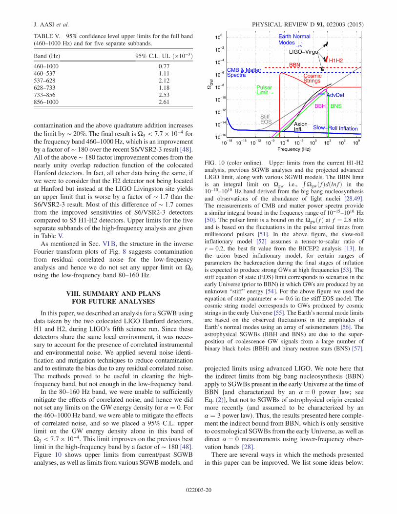
contamination and the above quadrature addition increasesthe limit by ∼ 20%. The final result is Ω3 < 7.7 × 10−4 forthe frequency band 460–1000 Hz, which is an improvementby a factor of ∼ 180 over the recent S6/VSR2-3 result [48].All of the above ∼ 180 factor improvement comes from thenearly unity overlap reduction function of the colocatedHanford detectors. In fact, all other data being the same, ifwe were to consider that the H2 detector not being locatedat Hanford but instead at the LIGO Livingston site yieldsan upper limit that is worse by a factor of ∼ 1.7 than theS6/VSR2-3 result. Most of this difference of ∼ 1.7 comesfrom the improved sensitivities of S6/VSR2-3 detectorscompared to S5 H1-H2 detectors. Upper limits for the fiveseparate subbands of the high-frequency analysis are givenin Table V.As mentioned in Sec. VI B, the structure in the inverse

Fourier transform plots of Fig. 8 suggests contaminationfrom residual correlated noise for the low-frequencyanalysis and hence we do not set any upper limit on Ω0

using the low-frequency band 80–160 Hz.

VIII. SUMMARY AND PLANSFOR FUTURE ANALYSES

In this paper, we described an analysis for a SGWB usingdata taken by the two colocated LIGO Hanford detectors,H1 and H2, during LIGO’s fifth science run. Since thesedetectors share the same local environment, it was neces-sary to account for the presence of correlated instrumentaland environmental noise. We applied several noise identi-fication and mitigation techniques to reduce contaminationand to estimate the bias due to any residual correlated noise.The methods proved to be useful in cleaning the high-frequency band, but not enough in the low-frequency band.In the 80–160 Hz band, we were unable to sufficiently

mitigate the effects of correlated noise, and hence we didnot set any limits on the GW energy density for α ¼ 0. Forthe 460–1000 Hz band, we were able to mitigate the effectsof correlated noise, and so we placed a 95% C.L. upperlimit on the GW energy density alone in this band ofΩ3 < 7.7 × 10−4. This limit improves on the previous bestlimit in the high-frequency band by a factor of ∼ 180 [48].Figure 10 shows upper limits from current/past SGWBanalyses, as well as limits from various SGWBmodels, and

projected limits using advanced LIGO. We note here thatthe indirect limits from big bang nucleosynthesis (BBN)apply to SGWBs present in the early Universe at the time ofBBN [and characterized by an α ¼ 0 power law; seeEq. (2)], but not to SGWBs of astrophysical origin createdmore recently (and assumed to be characterized by anα ¼ 3 power law). Thus, the results presented here comple-ment the indirect bound from BBN, which is only sensitiveto cosmological SGWBs from the early Universe, as well asdirect α ¼ 0 measurements using lower-frequency obser-vation bands [28].There are several ways in which the methods presented

in this paper can be improved. We list some ideas below:

TABLE V. 95% confidence level upper limits for the full band(460–1000 Hz) and for five separate subbands.

Band (Hz) 95% C.L. UL ð×10−3Þ460–1000 0.77460–537 1.11537–628 2.12628–733 1.18733–856 2.53856–1000 2.61

10−18

10−15

10−12

10−9

10−6

10−3

100

103

106

109

10−16

10−14

10−12

10−10

10−8

10−6

10−4

10−2

100

PulsarLimit

LIGO−Virgo

H1H2

Earth NormalModes

CMB & MatterSpectra

BBN

StiffEOS Axion

Infl.

CosmicStrings

BNSBBH

AdvDet

Slow−Roll Inflation

Frequency (Hz)

ΩG

W

FIG. 10 (color online). Upper limits from the current H1-H2analysis, previous SGWB analyses and the projected advancedLIGO limit, along with various SGWB models. The BBN limitis an integral limit on Ωgw i.e.,

RΩgwðfÞdðlnfÞ in the

10−10–1010 Hz band derived from the big bang nucleosynthesisand observations of the abundance of light nuclei [28,49].The measurements of CMB and matter power spectra providea similar integral bound in the frequency range of 10−15–1010 Hz[50]. The pulsar limit is a bound on the ΩgwðfÞ at f ¼ 2.8 nHzand is based on the fluctuations in the pulse arrival times frommillisecond pulsars [51]. In the above figure, the slow-rollinflationary model [52] assumes a tensor-to-scalar ratio ofr ¼ 0.2, the best fit value from the BICEP2 analysis [13]. Inthe axion based inflationary model, for certain ranges ofparameters the backreaction during the final stages of inflationis expected to produce strong GWs at high frequencies [53]. Thestiff equation of state (EOS) limit corresponds to scenarios in theearly Universe (prior to BBN) in which GWs are produced by anunknown “stiff” energy [54]. For the above figure we used theequation of state parameter w ¼ 0.6 in the stiff EOS model. Thecosmic string model corresponds to GWs produced by cosmicstrings in the early Universe [55]. The Earth’s normal mode limitsare based on the observed fluctuations in the amplitudes ofEarth’s normal modes using an array of seismometers [56]. Theastrophysical SGWBs (BBH and BNS) are due to the super-position of coalescence GW signals from a large number ofbinary black holes (BBH) and binary neutron stars (BNS) [57].

J. AASI et al. PHYSICAL REVIEW D 91, 022003 (2015)

022003-20

(i) As mentioned in Sec. IV C, we can improve theestimate of the PEM contribution to the coherenceby allowing for correlations between different PEMchannels ~zI and ~zJ. This requires inverting the fullmatrix of PEM coherences γIJðfÞ or solving a largenumber of simultaneous equations involving γIJðfÞ,rather than simply taking the maximum of theproduct of the coherences as was done here. Acomputationally cheaper alternative might be toinvert a submatrix formed from the largest PEMcontributors—i.e., those PEM channels that contrib-ute the most to the coherence.

(ii) We can use bicoherence techniques to account for(nonlinear) up-conversion processes missed by stan-dard coherence calculations. This may allow us toidentify cases where low-frequency disturbancesexcite higher-frequency modes in the detector.

(iii) The estimators Ω̂αðfÞ used in this analysis areoptimal in the absence of correlated noise. In thepresence of correlated noise, these estimators arebiased, with expected values given by the sum,Ωα þ ηαðfÞ, where the second term involves thecross spectrum, N12ðfÞ, of the noise contribution tothe detector output. An alternative approach is tostart with a likelihood function for the detectoroutput ~s1, ~s2, where we allow (at the outset) forthe presence of cross-correlated noise. (This wouldshow up in the covariance matrix for a multivariateGaussian distribution.) We can parametrize N12ðfÞin terms of its amplitude, spectral index, etc., andthen construct posterior distributions for theseparameters along with the amplitude and spectralindex of the stochastic GW signal. In this (Bayesian)approach, the cross-correlated noise is treated on thesame footing as the stochastic GW and is estimated(via its posterior distribution) as part of the analysis[58]. However, as described in [59], this works onlyfor those cases where the spectral shapes of the noiseand signal are different from one another.

(iv) We can also reduce correlated noise by first remov-ing as much noise as possible from the output of theindividual detectors. Wiener filtering techniques canbe applied to remove acoustic, magnetic, and grav-ity-gradient noise from the time-series output of theLIGO detectors [60–62]. Furthermore, feed-forward

control can be used to to cancel seismicallyinduced motion before it affects the LIGO testmasses [61].

These and/or other techniques might be needed for futurecross-correlation searches using advanced detectors, whereimproved (single-detector) sensitivity will mean that corre-lated noise may be an issue even for physically separateddetectors, such as the LIGO Hanford–LIGO Livingstondetector pair [29,30,63].

ACKNOWLEDGMENTS

The authors gratefully acknowledge the support of theU.S. National Science Foundation for the construction andoperation of the LIGO Laboratory, the Science andTechnology Facilities Council of the United Kingdom,the Max-Planck-Society, and the State of Niedersachsen/Germany for support of the construction and operation ofthe GEO600 detector, and the Italian Istituto Nazionale diFisica Nucleare and the French Centre National de laRecherche Scientifique for the construction and operationof the Virgo detector. The authors also gratefully acknowl-edge the support of the research by these agencies and bythe Australian Research Council, the International ScienceLinkages program of the Commonwealth of Australia, theCouncil of Scientific and Industrial Research of India, theIstituto Nazionale di Fisica Nucleare of Italy, the SpanishMinisterio de Economía y Competitividad, the Conselleriad'Economia Hisenda i Innovació of the Govern de les IllesBalears, the Foundation for Fundamental Research onMatter supported by the Netherlands Organisation forScientific Research, the Polish Ministry of Science andHigher Education, the FOCUS Programme of Foundationfor Polish Science, the Royal Society, the Scottish FundingCouncil, the Scottish Universities Physics Alliance, TheNational Aeronautics and Space Administration, OTKA ofHungary, the Lyon Institute of Origins (LIO), the NationalResearch Foundation of Korea, Industry Canada and theProvince of Ontario through the Ministry of EconomicDevelopment and Innovation, the National Science andEngineering Research Council Canada, the Carnegie Trust,the Leverhulme Trust, the David and Lucile PackardFoundation, the Research Corporation, and the Alfred P.Sloan Foundation.

[1] L. P. Grishchuk, JETP Lett. 23, 293 (1976).[2] A. A. Starobinskii, JETP Lett. 30, 682 (1979).[3] R. Bar-Kana, Phys. Rev. D 50, 1157 (1994).[4] M. Maggiore, Phys. Rep. 331, 283 (2000).[5] B. Abbott et al., Rep. Prog. Phys. 72, 076901 (2009).

[6] F. Acernese et al., Classical Quantum Gravity 25, 114045(2008).

[7] B. Willke et al., Classical Quantum Gravity 23, S207 (2006).[8] P. Bender, K. Danzmann, and the LISA Study Team, LISA

Project Report No. MPQ233, 1998.

SEARCHING FOR STOCHASTIC GRAVITATIONAL WAVES … PHYSICAL REVIEW D 91, 022003 (2015)

022003-21

[9] E. Phinney et al., The Big Bang Observer: DirectDetection of Gravitational Waves from the Birthof the Universe to the Present (NASA, Washington,D.C., 2004).

[10] F. A. Jenet, G. B. Hobbs, W. van Straten, R. N. Manchester,M. Bailes, J. P. W. Verbiest, R. T. Edwards, A. W. Hotan,J. M. Sarkissian, and S. M. Ord, Astrophys. J. 653, 1571(2006).

[11] R. van Haasteren et al., Mon. Not. R. Astron. Soc. 414,3117 (2011).

[12] B. Allen, in Proceedings of the Les Houches School onAstrophysical Sources of Gravitational Waves (CambridgeUniversity Press, Cambridge, England, 1997), p. 373.

[13] P. A. R. Ade et al. (BICEP2 Collaboration), Phys. Rev. Lett.112, 241101 (2014).

[14] R. Flauger, J. C. Hill, and D. N. Spergel, J. Cosmol.Astropart. Phys. 08 (2014) 039.

[15] M. J. Mortonson and U. Seljak, J. Cosmol. Astropart. Phys.10 (2014) 035.

[16] T. Regimbau and J. de Freitas Pacheco, Astron. Astrophys.447, 1 (2006).

[17] T. Regimbau and J. de Freitas Pacheco, Astron. Astrophys.376, 381 (2001).

[18] T. Regimbau and J. A. de Freitas Pacheco, Astrophys. J.642, 455 (2006).

[19] T. Regimbau and B. Chauvineau, Classical QuantumGravity 24, S627 (2007).

[20] X.-J. Zhu, E. Howell, T. Regimbau, D. Blair, and Z.-H. Zhu,Astrophys. J. 739, 86 (2011).

[21] A. Jaffe and D. Backer, Astrophys. J. 583, 616 (2003).[22] P. Michelson, Mon. Not. R. Astron. Soc. 227, 933 (1987).[23] N. Christensen, Phys. Rev. D 46, 5250 (1992).[24] E. E. Flanagan, Phys. Rev. D 48, 2389 (1993).[25] B. Allen and J. D. Romano, Phys. Rev. D 59, 102001

(1999).[26] B. Abbott et al., Phys. Rev. D 69, 122004 (2004).[27] B. Abbott et al., Astrophys. J. 659, 918 (2007).[28] B. Abbott et al., Nature (London) 460, 990 (2009).[29] E. Thrane, N. Christensen, and R. M. S. Schofield, Phys.

Rev. D 87, 123009 (2013).[30] E. Thrane, N. Christensen, R. M. S. Schofield, and A. Effler,

Phys. Rev. D 90, 023013 (2014).[31] B. Abbott et al., Nucl. Instrum. Methods Phys. Res., Sect. A

517, 154 (2004).[32] L. Blackburn et al., Classical Quantum Gravity 25, 184004

(2008).[33] N. Christensen, P. Shawhan, and G. González for (the LIGO

Scientific Collaboration), Classical Quantum Gravity 21,S1747 (2004).

[34] A. diCredico (for the LIGO Scientific Collaboration),Classical Quantum Gravity 22, S1051 (2005).

[35] N. Christensen (for the LIGO Scientific Collaboration),Classical Quantum Gravity 22, S1059 (2005).

[36] B. Abbott et al., Classical Quantum Gravity 24, 5343(2007).

[37] B. Abbott et al.., Phys. Rev. Lett. 102, 111102 (2009).[38] B. Abbott et al., Phys. Rev. D 80, 042003 (2009).[39] L. Grishchuk, Sov. Phys. Usp. 31, 940 (1988).[40] P. A. R. Ade et al., Astron. Astrophys. 571, A1 (2014).[41] For other pairs such as H1-L1, γðfÞ could be zero at some

frequencies. Since both Ω̂αðfÞ and σΩ̂αðfÞ have γðfÞ in their

denominators, the final result obtained by the weightedaverage [Eq. (7)] is always finite.

[42] For ease of notation, we do not explicitly show the timedependence of the estimators.

[43] N. V. Fotopoulos (for the LIGO Scientific Collaboration),J. Phys. Conf. Ser. 122, 012032 (2008).

[44] N. V. Fotopoulos (for the LIGO Scientific Collaboration),Classical Quantum Gravity 23, S693 (2006).

[45] S. Chatterji, L. Blackburn, G. Martin, and E. Katsavounidis,Classical Quantum Gravity 21, S1809 (2004).

[46] J. Abadie et al., Phys. Rev. D 85, 122001 (2012).[47] B. Abbott et al., Phys. Rev. Lett. 95, 221101 (2005).[48] J. Aasi et al. (LIGO Scientific and VIRGO Collaborations),

Phys. Rev. Lett. 113, 231101 (2014).[49] R. H. Cyburt, B. D. Fields, K. A. Olive, and E. Skillman,

Astropart. Phys. 23, 313 (2005).[50] I. Sendra and T. L. Smith, Phys. Rev. D 85, 123002 (2012).[51] R.M. Shannon, V. Ravi, W. A. Coles, G. Hobbs, M. J. Keith,

R. N. Manchester, J. S. B. Wyithe, M. Bailes, N. D. R. Bhat,S. Burke-Spolaor et al., Science 342, 334 (2013).

[52] M. S. Turner, Phys. Rev. D 55, R435 (1997).[53] N. Barnaby, E. Pajer, and M. Peloso, Phys. Rev. D 85,

023525 (2012).[54] L. A. Boyle and A. Buonanno, Phys. Rev. D 78, 043531

(2008).[55] X. Siemens, V. Mandic, and J. Creighton, Phys. Rev. Lett.

98, 111101 (2007).[56] M. Coughlin and J. Harms, Phys. Rev. D 90, 042005 (2014).[57] C. Wu, V. Mandic, and T. Regimbau, Phys. Rev. D 85,

104024 (2012).[58] E. Robinson and A. Vecchio, Report No. LIGO-P1100107,

2011.[59] M. R. Adams and N. J. Cornish, Phys. Rev. D 89, 022001

(2014).[60] B. Allen, W. Hua, and A. Ottewill, arXiv:gr-qc/9909083.[61] J. C. Driggers, M. Evans, K. Pepper, and R. Adhikari, Rev.

Sci. Instrum. 83, 024501 (2012).[62] J. C. Driggers, J. Harms, and R. X. Adhikari, Phys. Rev. D

86, 102001 (2012).[63] N. L. Christensen, Ph.D. thesis, Massachusetts Institute of

Technology, 1990.

J. AASI et al. PHYSICAL REVIEW D 91, 022003 (2015)

022003-22