Bayesian Melding of a

Forest Ecosystem Model with

Correlated Inputs

Philip J. Radtke, Thomas E. Burk, and Paul V. Bolstad

ABSTRACT. Bayesian melding, a method for assessing uncertainties in deterministic simulationmodels, was augmented to make use of prior knowledge about correlations between model inputs.The augmentation involved the use of a nonparametric correlation induction algorithm. The modifiedBayesian melding technique was applied to the process-based forest ecosystem computer modelPnET-ll. The Bayesian posterior distribution for this analysis did not reflect prior knowledge of inputcorrelations for five input pairs tested unless the correlations were explicitly accounted for in theBayesian prior distribution. For other input pairs not known to be correlated prior to the analysis,numerous significant posterior correlations were identified. For one such pair of model inputs, amoderate posterior correlation was substantiated by empirical evidence that had not previously beentaken into consideration. We conclude that, when possible, efforts should be made to account for priorknowledge of correlated inputs; however, Bayesian melding may elucidate input correlations in itsposterior sample, even when no prior knowledge of such correlations exists. FOR. Sci. 48(4):701-711.

Key Words: Bayesian melding, big leaf model, simulation, model evaluation, process model, Latinhypercube.

T HE USE OF PROCESS-BASED forest ecosystem computermodels has become commonplace for conductingresearch in the study of forest ecosystem dynamics.

Researchers have adopted the process-based modeling para-digm because it has some key advantages over traditionalstatistical modeling techniques. Chief among these are thestrengths of process-based models in the areas of knowledgesynthesis and predictive extrapolation. Still, widespread adop-tion of process-based models for practical applications hasbeen limited, mainly due to the lack of answers regarding themagnitudes of prediction uncertainty. Increasingly, attentionhas been paid to the need for quantitative assessments of thequality of predictions made with process-based computermodels (Cipra 2000, Makela et al. 2000).

Bayesian melding (BYSM) is a technique that allows forthe assessment of uncertainty in deterministic computermodel predictions by estimating Bayesian posterior distribu-tions of model inputs and outputs. As such, significantpotential exists to use BYSM for quantifying prediction

uncertainty in process-based forest ecosystem models. Themethod was developed by Raftery et al. (1995) to account foravailable information and uncertainty related to computermodel predictions of a population of an endangered whalespecies. The goal of their analysis was to develop probabilis-tic statements of how likely it would be that the whalepopulation might drop below some critical level following aproposed harvest of whales by aboriginal subsistence hunt-ers. To achieve this goal, the researchers developed thetheoretical framework and an algorithm for implementingwhat they called Bayesian synthesis.

Wolpert (1995) pointed out that Bayesian synthesis wassubject to Borel's paradox, meaning results were?"not invari-ant to rescaling of model outputs. Bayesian melding wasdeveloped to overcome this limitation (Poole and Raftery2000). The key result of BYSM is an approximation to theBayesian joint posterior distribution for model inputs. Thepropagation of this distribution through the model results inthe posterior distribution of outputs. Descriptive statistics—

Philip J. Radtke, Assistant Professor, Department of Forestry (0324), Virginia Tech, Blacksburg, VA 24061—Phone: (540) 231-8863; Fax: (540) 231-3698; E-mail: pradtke@vt.edu. Thomas E. Burk, Professor, Department of Forest Resources, University of Minnesota, 1530 Cleveland Ave N. St.Paul, MN 55108—Phone: (612) 624-6741; E-mail: tburk@forestry.umn.edu. Paul V. Bolstad, Associate Professor, Department of Forest Resources,University of Minnesota, 1530 Cleveland Ave N. St. Paul, MN 55108—Phone: (612) 625-1703; E-mail: pbolstad@forestry.umn.edu.Acknowledgments: The authors acknowledge the efforts of three anonymous reviewers, whose comments greatly improved earlier versions of this work.Manuscript received October 20, 2000, accepted August 22, 2001. Copyright © 2002 by the Society of American Foresters

Forest Science 48(4) 2002 701

modes, means, variances, intervals, etc.—can be readilyestimated from the posterior distributions of any subset ofmodel inputs or outputs. Because statistics based on regionsof highest Bayesian posterior density are generalized maxi-mum likelihood estimates (Berger 1985 p. 140-143), thedevelopment of BYSM represents something of a break-through in research on assessing the quality of process-modelpredictions.

To date, researchers have conducted BYSM analysesmaking a simplifying assumption in their formulations ofBayesian prior distributions: that model inputs are indepen-dent of one another. BYSM does not require this assumption,but it has typically been adopted to simplify implementationof the method where input relationships were unknown orwhere joint prior distributions for model inputs were difficultto formulate explicitly (Rafteryetal. 1995, Green etal. 1999,Poole and Raftery 2000). Interestingly, the results of BYSManalysis have been shown to elucidate relationships that existbetween model inputs a posteriori (Green et al. 1999). Still,in many situations, prior information about relationshipsbetween model inputs is known. It would seem desirable tomake use of such information when available. Ignoringrelationships between model parameters can be a serioussource of error in analyses that evaluate the quality of modelpredictions (Iman and Conover 1982, Guan 2000).

The objective here was to augment BYSM methodologyto take a priori account of correlations known to existbetween the inputs of a process-based computer model. Thisaugmentation would be developed and applied by conductingBYSM for the process-based forest ecosystem model PnET-II (Aber et al. 1995). PnET-II was designed to addressquestions involving regional, long-term dynamics of ecosys-tem water and carbon cycling. Because of this, PnET-II hasplayed a significant role in the modeling of regional forestecosystem dynamics and responses to predicted climatechange scenarios (McNulty et al. 1996, Goodale et al. 1998,Ollinger et al. 1998). A good deal is known about thedistributions of PnET-II model inputs, including empiricalevidence of correlations between some input pairs (Radtke etal. 2001).

The central question here is whether or not BYSM willaccurately predict correlations between PnET-II model in-puts in the posterior distribution, even though the priordistributions of inputs are assumed to be independent. Weproposed to answer this question by conducting BYSMassuming independence of inputs, and comparing results toBYSM conducted assuming a prior correlation structure. Thehypothesis to be tested from this approach was that BYSMposteriors would reflect correlations correctly, even whensuch correlations were not specified a priori.

MethodsBYSM was so named because of the prominence of

Bayes' theorem in the methodology and the fact that thetechnique combines or "melds" information from three sourcesin deriving its estimates of Bayesian posterior distributions(Poole and Raftery 2000). Sources of information are catego-rized as either direct or indirect, with the third source of

information being the model itself. Direct and indirect sourcesare distinguished by whether they are observed directly on apopulation of interest or obtained from outside sources some-how related to the population of interest. Direct and indirectinformation may pertain to either model inputs or outputs.Direct information typically involves a sample of observa-tions made on the population of interest. Indirect informationis expressed as probability density functions (PDFs) thatreflect knowledge and uncertainty about the varipus modelquantities.

BYSMBYSM is concerned with deterministic simulation mod-

els, particularly model inputs and outputs and functionsthereof. A brief description is included here for clarity andcompleteness. For additional detail and examples see Rafteryet al. (1995), Green et al. (1999), and Poole and Raftery(2000). A basic premise of BYSM is that information isavailable for some inputs and outputs, but there is likely to besome uncertainty associated with that information. The setsof model inputs and outputs for which we have informationindependent of the model are denoted by 9 and ()>, respec-tively, which are vectors for models that involve multipleinputs and outputs. Quantities of interest are not limited to 9and 4>. Indirect information translates to Bayesian priors, anddirect information translates to likelihoods. The premodelBayesian prior density for inputs is denoted <?e(9) and theBayesian prior density for outputs is denoted qM). Both<7e(9) and qM) are established before any execution of themodel is carried out. Likelihoods for inputs and outputs aredenoted £e(9) and LJ$), respectively. Subscripts 9 and <[>refer to model inputs and outputs, respectively. If we assumethat information about outputs is independent of informationabout the inputs, Bayes' theorem gives us the'followingposterior distribution.

Although (1) is a posterior in the Bayesian sense, it iscompiled without any consideration of the information con-tained in the model; thus,/?(9,40 is referred to as the jomtpre-model (posterior) distribution of 9 and <|>.

The model can be thought of as a mapping of inputs tooutputs: O(9) —> <(>. It follows that the joint post-model(posterior) distribution Jt(9, <|>) will have nonzero probabilityonly when <|> = <D(9). Raftery et al. (1995) defined the jointdistribution of 9 and <j> given the model as "the restriction ofthe pre-model distribution to the submanifold {(9, <|>): ((> =O(9)}," namely

(2)p(9,O(9)) if <t> =

0 otherwise

Resolving Borel's ParadoxIn implementing Bayesian synthesis, Raftery et al. (1995)

used the sampling importance resampling (SIR) algorithm ofRubin (1988) to approximate n(Q, <|>) so that inferences on thepost-model marginal distributions of inputs and outputs couldbe made. Wolpert (1995) pointed out that the joint distribu-

702 Forest Science 48(4) 2002

tion rc(0, ((>) in Equation (2) did not exist because of Borel'sparadox. This paradox arises in BYSM because <7e(0), whenpropagated through the model, implies a prior distribution onthe model outputs denoted q'e (<)>) and referred to as the priordistribution of outputs implied by the model and <79(0).Nothing in the method constrains q^ (()>) and qM) to be equal,effectively allowing for two conflicting priors to exist simul-taneously. Raftery et al. (1996) proposed a modification tothe method to eliminate Borel's paradox. Their solutioninvolved logarithmic pooling of the specified and impliedpriors into a single pooled prior for model outputs

4. Form importance sampling weights rk using (5) with a0.5 for geometric pooling.

>l-d

l-a (3)

where a is a pooling weight 0 < a < 1. When the two priorson the right hand side of (3) arise from the same base ofexpertise, a logical choice for a is 0.5. Other choices may beappropriate if input and output priors are based on differentexpertise bases and one expert is seen as more reliable thanthe other (Poole and Raftery 2000). When a = 0.5 is chosen,Equation (3) amounts to geometric pooling of the specifiedand implied priors for model outputs.

Assuming that inferences are to be made on inputs, thesame problem arises because #*(<)>), when propagated throughthe inverted model, implies a prior distribution on inputs thatwill surely contradict #e(0). The problem is further compli-cated when the model is not invertible, a certainty for modelsin which the number of outputs is smaller than the number ofinputs. The ideal solution involves obtaining a pooled priorfor inputs, ^8](0), by inverting q^(§) backwards throughthe model. For values of <j> that map to multiple points in 0, thedensity of those points is distributed in proportion to the priordensity ^e(0). Poole and Raftery (2000) showed that theproper way to arrive at ̂ '^(0), whether or not the model isinvertible, is by the following formula

(4)

Implementation: SIRRaftery et al. (1996) proposed a modification to the SIR

algorithm to implement BYSM with geometric pooling so asto eliminate Borel's paradox. The modified SIR algorithm iscarried out in the following five steps (Raftery and Poole1997), which are reviewed here for completeness.

1. Draw a random sample of size M from the values of 0 fromits prior distribution <7e(0). Denote the sample by (0];

02,..,0M).

2. For each value of Qk sampled in step 1, run the model toobtain the corresponding value of §k = <&(&%).

3. Use nonparametric density estimation to obtain an esti-mate of q^ (<j>), the resulting model-implied density of <)>for {<|>|, <j>2, ... ,<|>^}. Kernel density estimation with aGaussian kernel has the advantage of being easily appliedin higher dimensions (Silverman 1986, Scott 1992). Thewindow width of the smoother was chosen by the normalreference rule (Scott 1992, p. 131).

(5)

5. Sample m values, with replacement, from the discretedistribution of M values of (Qk, (|>t) and sampling prob-abilities proportional to rk

When Mlm is large, the result of SIR step 5 is an approxi-mate sample from the geometrically pooled, post-modelposterior distribution. It can be used to make inferences aboutquantities of interest, which may involve inputs or outputs orfunctions thereof.

Accounting for CorrelationsTo account for correlated model inputs analytically would

require specifying a joint prior distribution for all inputs. Forsome situations this would be a reasonable task, assumingmathematically tractable PDFs were available to describe thejoint distributions (e.g., bivariate normal distributions). Inpractice this will often be problematic as the number of inputsis large and joint relationships are not always easily defined.We used a nonparametric method that accounts for rankcorrelations between inputs rather than parametric specifica-tion ofmultivariate relationships. The method was developedfor inducing correlations in random samples of model inputsfor Latin Hypercube Sampling (Iman and Conover 1980).Iman and Conover (1982) described the correlation inductionalgorithm in detail, including numerical examples. A briefoverview explaining how the method is implemented inBYSM follows.

Correlations are induced immediately following SIR step1. In step 1, a large number (M) of input values are randomlygenerated for each of the P model inputs for which Bayesianpriors are available. For convenience, the simulated valuesare arranged in a M x P data matrix D. The columns of D arerandom samples from the marginal priors of 0. A P x Ppositive definite target rank correlation matrix R is specified.The restriction that R be positive definite is due to thecomputation of the Cholesky decomposition of R in thecorrelation induction algorithm. Correlations are induced bypartially sorting the columns of D to attain the target correla-tion structure. Since the algorithm only mixes values withinthe columns of D, all marginal distributions are^preserved.The rearranged data matrix D will have a correlation structureidentical to R. Although the augmentation to SIR step 1 doesnot completely specify a joint distribution for ge(0), it doeshave the desirable effect of accounting for correlations be-tween the inputs. SIR proceeds with the sample of A/modelinput vectors that satisfy the target correlation structure.

Additional consideration for correlated inputs may benecessary in SIR step 4. Calculations of likelihoods involvinginputs must account for the desired correlation structure. Ifdata pairs (triplets, etc.) directly observed on the populationof interest were available for inputs assumed a priori to becorrelated, explicit formulas for their joint likelihood wouldbe needed in SIR step 4 [Equation (5)] .If no directly observed

Forest Science 48(4) 2002 703

data were available for the correlated inputs, likelihoodcalculations involving these inputs would not be necessary.

DataHaving chosen to work with the model PnET-II, we

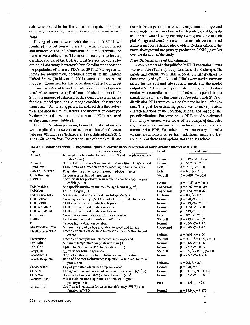
identified a population of interest for which various directand indirect sources of information about model inputs andoutputs were obtainable. The mixed-species, broadleaved,deciduous forest of the USDA Forest Service Coweeta Hy-drologic Laboratory in western North Carolina was chosen asthe population of interest. PDFs for 29 PnET-II vegetationinputs for broadleaved, deciduous forests in the EasternUnited States (Radtke et al. 2001) served as a source ofindirect information for this population (Table 1). Indirectinformation relevant to soil and site-specific model quanti-ties for Coweeta was compiled from published sources (Table2) for the purpose of establishing data-based Bayesian priorsfor these model quantities. Although empirical observationswere used in formulating priors, the indirect data themselveswere not used in BYSM. Rather, the information conveyedby the indirect data was compiled as a set of PDFs to be usedas Bayesian priors (Table 3).

Direct information pertaining to model inputs and outputswas compiled from observational studies conducted at Coweetabetween 1987 and 1995 (Bolstadetal. 1998,Bolstadetal. 2001).The available data from Coweeta consisted of complete climate

records for the period of interest, average annual foliage, andwood production values observed at 16 study plots at Coweetaand the soil water holding capacity (WHC) measured at eachplot. Foliage and wood biomass production data were summedand averaged for each field plot to obtain 16 observations of themean aboveground net primary production (ANPP, g/m2/yr)over the duration of the study.

Prior Distributions and CorrelationsA complete set of prior pdfs for PnET-II vegetation inputs

was available (Table 1), but priors for soil and site-specificinputs and outputs were still needed. Similar methods tothose employed by Radtke et al. (2001) were usedjo estimatepriors for the soil and site-specific inputs and the modeloutput ANPP. To estimate prior distributions, indirect infor-mation was compiled from published studies pertaining topopulations similar to the forests at Coweeta (Table 2). Priordistribution PDFs were estimated from the indirect informa-tion. The goal for estimating priors was to make practicalcharacterizations of the location, spread, and shape of theprior distributions. For some inputs, PDFs could be estimatedfrom simple summary statistics of the compiled data sets,e.g., the mean and variance of the indirect observations for anormal prior PDF. For others it was necessary to makevarious assumptions or perform additional analyses. De-scriptions of these assumptions and analyses follow.

Table 1. Distributions of PnET-II vegetation inputs for eastern deciduous forests of North America (Radtke et al. 2001).InputAmaxA

AmaxBAmaxFracBaseFolRespFracCfracBiomassDVPD1

FolMassMaxFolNConFolRelGrowMaxGDDFolEndGDDFolStartGDDWoodEndGDDWoodStartGrespFracHalfSatkMinWoodFolRatioPlantCReserveFrac

PrecIntFracPsnTMinPsnTOptRespQIORootAllocBRootMRespFrac

SenesceStartSLWDelSLWMaxWoodMRespA

WueConst

Definition (units)Intercept of relationship between foliar N and max photosynthetic

rate (Amax)Slope of Amax versus N relationship; Amax (umol CO2/g leaf/s)Daily Amax as a fraction of early morning instantaneous rateRespiration as a fraction of maximum photosynthesisCarbon as a fraction of tissue massCoefficients for photosynthesis reduction due to vapor pressure

deficit (VPD)Site specific maximum summer foliage biomass (g/m2)Foliar nitrogen (%)Maximum relative growth rate for foliage (% /yr)Growing degree days (GDD) at which foliar production endsODD at which foliar production beginsGDD at which wood production endsGDD at which wood production beginsGrowth respiration, fraction of allocated carbonHalf saturation light intensity (umol/mVs)Canopy light extinction constantMinimum ratio of carbon allocation to wood and foliageFraction of plant carbon held in reserve after allocation to bud

carbonFraction of precipitation intercepted and evaporatedMinimum temperature for photosynthesis (°C)Optimum temperature for photosynthesis (°C)Q10 value for foliar respirationSlope of relationship between foliar and root allocationRatio of fine root maintenance respiration to fine root biomass

productionDay of year after which leaf drop can occurChange in SLW with accumulated foliar mass above (g/m2/g)Specific leaf weight (SLW) at top of canopy (g/m2)Wood maintenance respiration as a fraction of gross

photosynthesisCoefficient in equation for water use efficiency (WUE) as a

function of VPD

Family

NormalNormalBetaBetaWeibull

NormalLognormalLognormalUniformNormalNormalNormalNormalBetaWeibullNormalLognormal

UniformWeibullNormalNormalWeibullNormal

UniformNormalNormalNormal

Beta

Normal

Distribution

u = -12.2, 0=15.4u = 62.7, 0 = 7.0a = 23.2, (3 = 7.30a = 6.0, p = 37.3P = 0.494, 7 =35.4

u = -0.43, 0 = 0.011u = 5.76, a = 0.34!)u = 0.74, o = 0.26'a = 0.2,p = 0.5u = 898, o=189u = 379, o=75 'u= 1158,0 = 238\i = 639, 0=132a = 8.2,P = 23.0P = 299.9,Y=1.87H = 0.56, o = 0. 12u = 0.46, o = 0.42

a = 0.05, p = 0.95'<x = 0.11,p = 0.05,7=1.8u = 0.68, o = 0.64H = 22.2, 0 = 0.33a = 1.9, P = 0.60,7=1.87u = 2.52, o = 0.214

a = 0.5,P = 2.0u = 260,a=13u = -0.1 55, 0 = 0.014u= 87.2, o=18.8

a = 12.4, P = 99.8

u= 10.9, 0 = 0.875

704 Forest Science 48(4) 2002

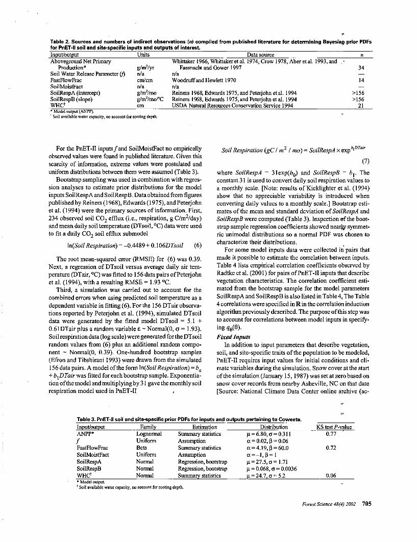
•Table 2. Sources and numbers of indirect observations (n) compiled from published literature for determining Bayesiag prior PDFsfor PnET-ll soil and site-specific inputs and outputs of interest.Input/outputAboveground Net Primary

Production*Soil Water Release Parameter (f)FastFlowFracSoilMoistFactSoilRespA (intercept)SoilRespB (slope)WHCf

Units

g/m2/yrn/acm/cmn/ag/m2/mog/m2/mo/°Ccm

Data sourceWhittakerl966,Whittakeretal. 1974, Crow 1978, Aberetal. 1993,and •

Fassnacht and Gower 1997n/aWoodruff and Hewlett 1970n/aReiners 1968, Edwards 1975, andPeterjohn etal. 1994Reiners 1968, Edwards 1975, andPeterjohn etal. 1994USDA Natural Resources Conservation Service 1994

n

34

14

>156>156

21•Model output (ANPP).t Soil available water capacity, no account for rooting depth.

For the PnET-II inputs/and SoilMoistFact no empiricallyobserved values were found in published literature. Given thisscarcity of information, extreme values were postulated anduniform distributions between them were assumed (Table 3).

Bootstrap sampling was used in combination with regres-sion analyses to estimate prior distributions for the modelinputs SoilRespA and SoilRespB. Data obtained from figurespublished by Reiners (1968), Edwards (1975), and Peterjohnet al. (1994) were the primary sources of information. First,234 observed soil C02 efflux (i.e., respiration, g C/m2/day)and mean daily soil temperature (DTsoil, °C) data were usedto fit a daily CO2 soil efflux submodel

\n(Soil Respiration) = -0.4489 + 0.106DTsoil (6)

The root mean-squared error (RMSE) for (6) was 0.39.Next, a regression of DTsoil versus average daily air tem-perature (DTair, °C) was fitted to 156 data pairs of Peterjohnet al. (1994), with a resulting RMSE = 1.93 °C.

Third, a simulation was carried out to account for thecombined errors when using predicted soil temperature as adependent variable in fitting (6). For the 156 DTair observa-tions reported by Peterjohn et al. (1994), simulated DTsoildata were generated by the fitted model DTsoil = 5.1 +0.61DTair plus a random variable e ~ Normal(0, o = 1.93).Soil respiration data (log scale) were generated for the DTsoilrandom values from (6) plus an additional random compo-nent ~ Normal(0, 0.39). One-hundred bootstrap samples(Efron and Tibshirani 1993) were drawn from the simulated156 data pairs. A model of the form ln(Soil Respiration) = b0

+ b^DTair was fitted for each bootstrap sample. Exponentia-tion of the model and multiplying by 31 gave the monthly soilrespiration model used in PnET-II «

Soil Respiration (gC/m2 / mo) = SoilRespA x expbtDTair

(7)

where SoilRespA = 31exp(&0) and SoilRespB = b{. Theconstant 31 is used to convert daily soil respiration values toa monthly scale. [Note: results of Kicklighter et al. (1994)show that no appreciable variability is introduced whenconverting daily values to a monthly scale.] Bootstrap esti-mates of the mean and standard deviation of SoilRespA andSoilRespB were computed (Table 3). Inspection ef the boot-strap sample regression coefficients showed nearly symmet-ric unimodal distributions so a normal PDF was chosen tocharacterize their distributions.

For some model inputs data were collected in pairs thatmade it possible to estimate the correlation between inputs.Table 4 lists empirical correlation coefficients observed byRadtke et al. (2001) for pairs of PnET-II inputs that describevegetation characteristics. The correlation coefficient esti-mated from the bootstrap sample for the model parametersSoilRespA and SoilRespB is also listed in Table 4,.The Table4 correlations were specified in R in the correlation inductionalgorithm previously described. The purpose of this step wasto account for correlations between model inputs in specify-ing 98(

6)-Fixed Inputs

In addition to input parameters that describe vegetation,soil, and site-specific traits of the population to be modeled,PnET-II requires input values for initial conditions and cli-mate variables during the simulation. Snow cover at the startof the simulation (January 15,1987) was set at zero based onsnow cover records from nearby Asheville, NC on that date[Source: National Climate Data Center online archive (ac-

Table 3. PnET-II soil and site-specific prior PDFs for inputs and outputs pertaining to Coweeta.Input/output Family Estimation Distribution

* Model output.1 Soil available water capacity, no account for rooting depth.

KStestP-valueANPP*/FastFlowFracSoilMoistFactSoilRespASoilRespBWHCf

LognormalUniformBetaUniformNormalNormalNormal

Summary statisticsAssumptionSummary statisticsAssumptionRegression, bootstrapRegression, bootstrapSummary statistics

u = 6.80, 0 = 0.311a = 0.02, p = 0.06a = 4.19, P = 60.0a = -l ,p= 1u = 27.5,o=1.71u = 0.068, 0 = 0.0036u = 24.7, 0 = 5.2

0.77

0.72

0.06

Forest Science 48(4) 2002 705

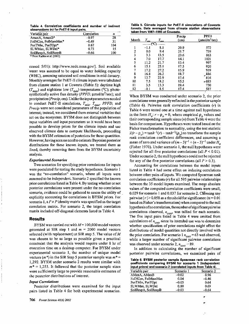
Table 4. Correlation coefficients and number of indirectobservations (n) for PnET-II input pairs.Variable pairAmaxA, AmaxB*FolNCon, FolMassMax*PsnTMin, PsnTOpt*SLWMax, SLWDel*SoilRespA, SoilRespB

Correlation-0.97-0.49

0.670.73

-0.66

n2831

10415

100* From Radtkeetal. (2001).

Table 5. Climate inputs for PnET-ll simulations of Coweetaforests. Data averaged from climate station observationstaken from 1987-1995 at Coweeta.

cessed 5/01): http://www.ncdc.noaa.gov/]. Soil availablewater was assumed to be equal to water holding capacity(WHC), assuming saturated soil conditions in mid-January.Monthly averages for PnET-II climate inputs were tabulatedfrom climate station 1 at Coweeta (Table 5): daytime high(Tmax) and nighttime low (Tmin) temperatures (°C); photo-synthetically active flux density (PPFD, (J.mol/m2/sec); andprecipitation (Precip, cm). Unlike the inputparameters neededto conduct PnET-II simulations, Tmia, Tmax, PPFD, andPrecip were not considered parameters of the population ofinterest; instead, we considered them external variables thatact on the ecosystem. BYSM does not distinguish betweeninput variables and input parameters so it would have beenpossible to develop priors for the climate inputs and useobserved climate data to compute likelihoods, proceedingwith the BYSM estimation of posteriors for these quantities.However, having seen no need to estimate Bayesian posteriordistributions for these known inputs, we treated them asfixed, thereby removing them from the BYSM uncertaintyanalysis.Experimental Scenarios

Two scenarios for specifying prior correlations for inputswere postulated for testing the study hypotheses. Scenario 1was the "no-correlation" scenario, where all inputs wereassumed to be independent. Scenario 2 specified the knownprior correlations listed in Table 4. By testing whether or notposterior correlations were present under the no-correlationscenario, evidence could be gathered to assess the utility ofexplicitly accounting for correlations in BYSM priors. Forscenario 1, a P x P identity matrix was specified as the targetcorrelation matrix. For scenario 2, the target correlationmatrix included off-diagonal elements listed in Table 4.

ResultsBYSM was carried out with M= 100,000 model vectors

generated at SIR step 1 and m = 2000 model vectorsselected (with replacement) at SIR step 5. The value of Mwas chosen to be as large as possible given a practicalconstraint that the analysis would require under 8 hr ofexecution time on a desktop computer. For BYSM underexperimental scenario 1, the number of unique modelvectors (m*) in the SIR Step 5 posterior sample was m* =1,292. BYSM under scenario 2 results were similar withm* = 1,253. It followed that the posterior sample sizeswere sufficiently large to provide reasonable estimates ofthe posterior distributions of interest.

Input CorrelationsPosterior distributions were examined for the input

pairs listed in Table 4 for both experimental scenarios.

Month rmin rra,,

123456789

101112

CQ-1.1

0.03.37.0

11.215.117.216.813.77.53.5

-0.1

8.19.4

13.517.721.725.127.226.222.918.213.38.5

Precip(cm)

20.921.723.614.113.417.515.918.717.415.519.417.4

PPFD(umol/nvVsec)

572739863

1021997920939

,886816

»885730587

When BYSM was conducted under scenario 2, the priorcorrelations were generally reflected in the posterior sample(Table 6). Pairwise rank correlation coefficients (r) inTable 6 were tested one at a time against null hypothesesin the form H0: r - p0 = 0, where empirical p0 values andtheir corresponding sample sizes (n) from Table 4 were thebasis for comparison. Hypotheses were tested based on theFisher transformation to normality, using the test statisticZ(r - p0) = tanh~l(r) - tan/j~'(p0) to transform the samplerank correlation coefficient differences, and assuming amean of zero and variance of (m — 3)~l +(n-3)~1 under Hg

(Fisher 1970). Under scenario 1, the null hypotheses wererejected for all five posterior correlations (all P < 0.01).Under scenario 2, the null hypotheses could not be rejectedfor any of the five posterior correlations (all P > 0.3).

Accounting for correlations between the model inputslisted in Table 4 had some effect on inducing correlationsbetween other pairs of inputs. We computed Spearman rankcorrelation coefficients (r) for all 595 pairwise relationshipsbetween the 35 model inputs examined. The mean absolutevalues of the computed correlation coefficients were small,0.029 for scenario 1 and 0.037 for scenario 2. CHoosing anypairwise \r\> 0.058 as a threshold for significance (a = 0.01based on Fisher's transformation) when compared to the nullhypothesis of no correlation, the number of significantpairwisecorrelations observed, «corr, was tallied for each scenario.The five input pairs listed in Table 4 were omitted fromcalculations of «corr since its intended use was to determinewhether specification of prior correlations might affect thedistributions of model quantities not directly involved withthe prior correlation. For scenario 1 «corr = 63 was observed,while a larger number of significant pairwise correlationswas observed under scenario 2, ncorr = 89.

In addition to calculating the number of significantposterior pairwise correlations, we examined pairs of

Table 6. BYSM posterior sample Spearman rank correlationcoefficients comparing BYSM for scenario 1 (independentinput priors) and scenario 2 (correlated inputs from Table 4).Variable pairAMaxA, AMaxBFolNCon, FolMassMaxPsnTMin, PsnTOptSLWMax, SLWDelSoilRespA, SoilRespB

Scenario 1-0.02

0.04-0.05

0.00-0.03

Scenario 2-0.96-0.46

0.640.69

-0.64

706 Forest Science 48(4) 2002

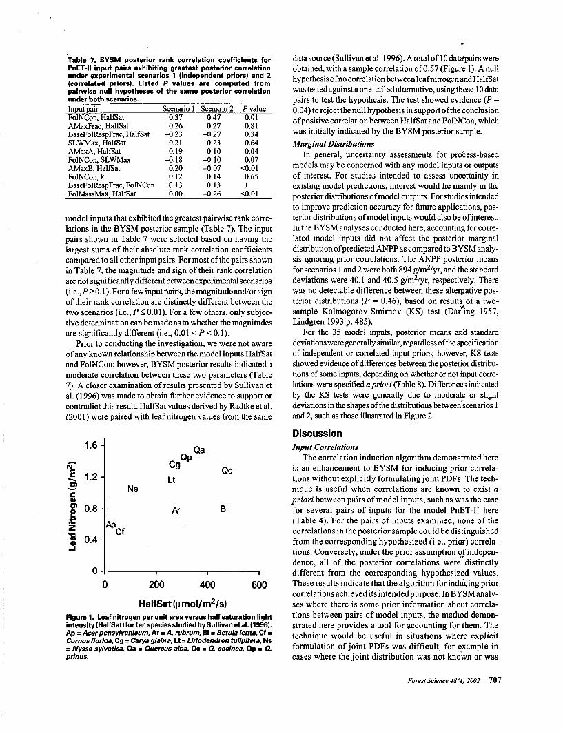
Table 7. BYSM posterior rank correlation coefficients forPnET-ll input pairs exhibiting greatest posterior correlationunder experimental scenarios 1 (independent priors) and 2(correlated priors). Listed P values are computed frompairwise null hypotheses of the same posterior correlationunder both scenarios.Input pairFolNCon, HalfSatAMaxFrac, HalfSatBaseFolRespFrac, HalfSatSLWMax, HalfSatAMaxA, HalfSatFolNCon, SLWMaxAMaxB, HalfSatFolNCon, kBaseFolRespFrac, FolNConFolMassMax, HalfSat

Scenario 10.370.26

-0.230.210.19

-0.180.200.120.130.00

Scenario 20.470.27

-0.270.230.10

-0.10-0.07

0.140.13

-0.26

P value0.010.810.340.640.040.07

<0.010.651

<0.01

model inputs that exhibited the greatest pairwise rank corre-lations in the BYSM posterior sample (Table 7). The inputpairs shown in Table 7 were selected based on having thelargest sums of their absolute rank correlation coefficientscompared to all other input pairs. For most of the pairs shownin Table 7, the magnitude and sign of their rank correlationare not significantly different between experimental scenarios(i.e., P > 0.1). For a few input pairs, the magnitude and/or signof their rank correlation are distinctly different between thetwo scenarios (i.e., P < 0.01). For a few others, only subjec-tive determination can be made as to whether the magnitudesare significantly different (i.e., 0.01 < P < 0.1).

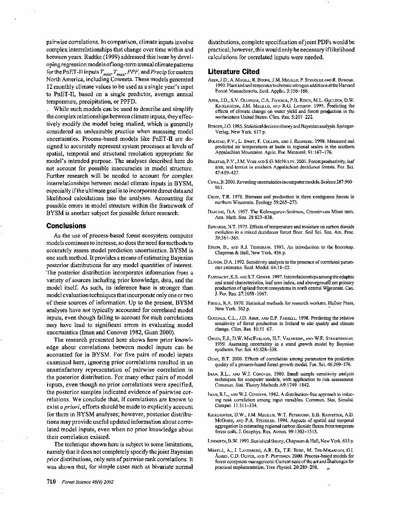
Prior to conducting the investigation, we were not awareof any known relationship between the model inputs HalfSatand FolNCon; however, BYSM posterior results indicated amoderate correlation between these two parameters (Table7). A closer examination of results presented by Sullivan etal. (199.6) was made to obtain further evidence to support orcontradict this result. HalfSat values derived by Radtke et al.(2001) were paired with leaf nitrogen values from the same

1.6-

5?o>§> 0.8-

Zg 0.4-

Ns

Cg

Lt

Ar

QpQa

Qc

Bl

Ap

200 400 600

HalfSat (umol/m2/s)Figure 1. Leaf nitrogen per unit area versus half saturation lightintensity (HalfSat) for ten species studied by Sullivan et al. (1996).Ap = Acer pensylvanicum, Ar = A. rubrum, Bl = Betula lenta, Cf =Cornus florida, Cg = Carya glabra, Lt = Liriodendron tulipifera, Ns= Nyssa sylvatica, Qa = Quercus alba, Qc = Q. cocinea. Qp = Q.prinus.

data source (Sullivan et al. 1996). A total of 10 datsfpairs wereobtained, with a sample correlation of 0.57 (Figure 1). A nullhypothesis of no correlation between leaf nitrogen and HalfSatwas tested against a one-tailed alternative, using these 10 datapairs to test the hypothesis. The test showed evidence (P =0.04) to reject the null hypothesis in support of the conclusionof positive correlation between HalfSat and FolNCon, whichwas initially indicated by the BYSM posterior sample.

Marginal DistributionsIn general, uncertainty assessments for process-based

models may be concerned with any model inputs or outputsof interest. For studies intended to assess uncertainty inexisting model predictions, interest would lie mainly in theposterior distributions of model outputs. For studies intendedto improve prediction accuracy for future applications, pos-terior distributions of model inputs would also be of interest.In the BYSM analyses conducted here, accounting for corre-lated model inputs did not affect the posterior marginaldistribution of predicted ANPP as compared to BYSM analy-sis ignoring prior correlations. The ANPP posterior meansfor scenarios 1 and 2 were both 894 g/m2/yr, and the standarddeviations were 40.1 and 40.5 g/m2/yr, respectively. Therewas no detectable difference between these alternative pos-terior distributions (P = 0.46), based on results of a two-sample Kolmogorov-Smirnov (KS) test (Darling 1957,Lindgren 1993 p. 485).

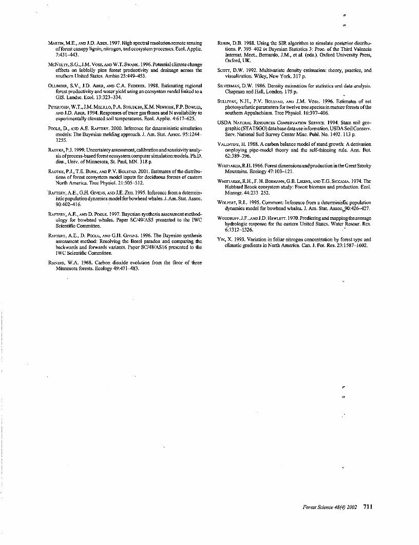
For the 35 model inputs, posterior means and standarddeviations were generally similar, regardless of the specificationof independent or correlated input priors; however, KS testsshowed evidence of differences between the posterior distribu-tions of some inputs, depending on whether or not input corre-lations were specified a priori (Table 8). Differences indicatedby the KS tests were generally due to moderate or slightdeviations in the shapes of the distributions betweenscenarios 1and 2, such as those illustrated in Figure 2.

DiscussionInput Correlations

The correlation induction algorithm demonstrated hereis an enhancement to BYSM for inducing prior correla-tions without explicitly formulating joint PDFs. The tech-nique is useful when correlations are known to exist apriori between pairs of model inputs, such as was the casefor several pairs of inputs for the model PnET-II here(Table 4). For the pairs of inputs examined, none of thecorrelations in the posterior sample could be distinguishedfrom the corresponding hypothesized (i.e., prior) correla-tions. Conversely, under the prior assumption of indepen-dence, all of the posterior correlations were distinctlydifferent from the corresponding hypothesized values.These results indicate that the algorithm for inducing priorcorrelations achieved its intended purpose. In BYSM analy-ses where there is some prior information about correla-tions between pairs of model inputs, the method demon-strated here provides a tool for accounting for them. Thetechnique would be useful in situations where explicitformulation of joint PDFs was difficult, for example incases where the joint distribution was not known or was

Forest Science 48(4) 2002 707

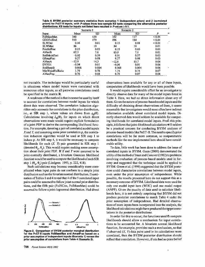
Table 8. BYSM posterior summary statistics from scenarios 1 (independent priors) and 2 (correlatedpriors) for PnET-ll inputs, with P-values from two-sample KS tests comparing the alternative posteriordistributions. KS tests for inputs not listed here resulted in P-values > 0.1.

InputFolMassMaxGDDFoIEndSLWDelSLWMaxPrecIntFracAMaxBSoilMoistFactGRespFracAMaxADVPD1SoilRespBMinWoodFolRatioAMaxFrac

ScenarioMean

340910

0.16860.15

62.3-0.02

0.27-12.9-0.04

0.0681.790.76

1SD

120179

0.01190.037.00.590.08

14.30.010.0040.780.08

ScenarioMean

352896

0.15840.15

63.00.010.27

-12.8-0.04

0.0681.740.75

2SD

117184

0.01180.037.10.570.08

15.70.010.0040.740.07

P<0.01<0.01<0.01

0.010.010.010.030.030.040.060.060.070.08

not tractable. The technique would be particularly usefulin situations where model inputs were correlated withnumerous other inputs, as all pairwise correlations couldbe specified in the matrix R.

A weakness of the method i s that it cannot be used by itselfto account for correlations between model inputs for whichdirect data were observed. The correlation induction algo-rithm only accounts for correlations in the prior distribution,i.e., at SIR step 1, where values are drawn from qe(Q).Calculations involving LQ(Q), for inputs on which directobservations were made would require explicit formulationof a joint PDF to derive the corresponding likelihood func-tion. For example, denoting a pair of correlated model inputsXand Y, and assuming some prior correlation p, the correla-tion induction algorithm would be used at SIR step 1 toinduce p. At SIR step 4, it would be necessary to computelikelihoods for each (X, Y) pair generated in SIR step 1(denoted 0X, 6 ). This would require making some assump-tion about their joint PDF. If X and Fwere assumed to bejoint-normally distributed, a bivariate Gaussian likelihoodfunction would be used to compute the likelihood of each SIRstep 1 (6X, ep pair (Lindgren 1993, p. 222,418).

Such calculations may become considerably more com-plicated when input pairs do not conform to a simple jointdistribution such as the bivariate normal distribution. Exami-nation of Tables 1 and 4 reveal that 4 of the 5 correlated inputpairs could be assumed to follow joint-normal prior distribu-tions, and the fifth pair (FolNCon, FolMassMax) could beassumed to follow a joint-lognormal distribution. Had direct

Scenario 1Scenario 2

800 0.6 0.8AMaxFrac

Figure 2. Comparison of BYSM posterior marginal distributionfor the PnET-ll inputs FolMassMax and AmaxFrac based on aprior assumption of independent inputs (Scenario 1) versus theprior assumption of correlations from Table 4 (Scenario 2).

observations been available for any or all of these inputs,computation of likelihoods would have been possible.

It would require considerable effort for an investigator todirectly observe data for many of the model inputs listed inTable 4. Here, we had no direct information about any ofthem. Given the nature of process-based model inputs and thedifficulty of obtaining direct observations of them, it seemsreasonable that investigators would most often have indirectinformation available about correlated model inputs. Di-rectly observed data would seldom be available for comput-ing likelihoods for correlated model inputs. From this prin-ciple, it follows that joint-likelihood calculations Will seldombe a practical concern for conducting BYSM analyses ofprocess-based models like PnET-II. The need to specify priorcorrelations will be far more common, so nonparametricmethods like the one implemented here should have consid-erable utility.

To date, little work has been done to address the issue ofcorrelated inputs in BYSM. Guan (2000) demonstrated theutility of the method of Iman and Conover (1982) to problemsinvolving evaluation of process-based models used in for-estry and suggested that the technique could be applied toBYSM. Green et al. (1999) suggested that the BYSM poste-riors could characterize correlations between model inputs,even under the prior assumption of independence. Whilepossible, the results presented here do not support this as anecessary outcome of BYSM. Likelihood data were used foronly one model input here (WHC) and one model output(ANPP). Given the paucity of data used to calculate likeli-hoods here, it is not entirely surprising that BYSM did notproduce posterior correlations to match Table 4 under theprior assumption of independence. Had detailed observa-tions of more inputs been incorporated into the analysis, thelikelihood calculations might have produced the target corre-lations in the posterior distributions.

In order for this to occur, the functions used tb computelikelihoods should allow a mechanism for input correla-tions to be accounted for. A bivariate normal likelihoodfunction, for example, provides such a mechanism, so thatif observed (X, Y) data pairs used in its calculations werecorrelated, then the BYSM posterior distribution shouldreflect that correlation. However, if one had no prior belief

708 Forest Science 48(4)2002

that X and Y were correlated, it would be reasonable toformulate their likelihoods as the product of two indepen-dent normal likelihood functions. Thus, it becomes appar-ent that simply including direct observations of A'and 7 inthe BYSM might not produce any posterior correlationbetween X and Y. In either case of having available directobservations or not, it would seem prudent to account forcorrelations as explicitly as possible in the specification ofprior distributions and likelihoods.

Although the BYSM analysis conducted here did notgenerate the hypothesized correlations for targeted inputs ofits own accord, significant (nonzero) posterior correlations.were observed for nontargeted model inputs. The numbers ofsignificant correlations were small compared to the findingsof Green et al. (1999), who observed significant relationshipsamong 44% of all possible input pairs tested at the a = 0.01level for the PIPESTEM model (Valentine 1998). The aver-age magnitude of the absolute values of posterior correlationswas also smaller here, around 0.03, compared to Green et al.(1999), who observed a value of 0.14. Their posterior samplesize was considerably larger (m = 5000), and they testedfewer pairwise correlations (276), thus the probability ofspurious nonzero correlations in theirposterior sample shouldhave been relatively small.

The possibility of spurious nonzero correlations should beconsidered, especially since pairwise tests of significancewere used to test against the null hypotheses of independence.One would expect a Type I error rate of 1 in 100 (a = 0.01),which corresponds to roughly 6 Type I errors when conduct-ing 595 pairwise tests, as was done here. The same number ofType I misclassifications would be expected under eitherscenario 1 or 2, so the comparison between the two «corr

values should not be affected by this problem. One factor thatmay help to minimize Type I errors in testing posteriorcorrelations is the use of the identity matrix for R whengenerating the SIR step 1 sample. Specifying R as the identity.matrix effectively removes any nonzero correlations thatmay have occurred by random chance in generating the SIRstep 1 values.

Regardless of whether input correlations were known toexist a priori, the BYSM posterior sample provides updatedinformation about the joint distributions of any model inputsof interest. The nonzero values of ncotT observed under bothexperimental scenarios indicate that prior beliefs about inde-pendence of inputs can be re-examined for possible updatinga posteriori. Information about such relationships may beuseful for a variety of applications such as subsequent uncer-tainty assessments or sensitivity analysis (Elston 1992, Guan2000). Posterior relationships may also provide informationabout actual relationships in the system being modeled. Suchresults may form the basis for hypotheses to be tested infuture research, such as the hypothesis that HalfSat andFolNCon are positively correlated in broadleaved, deciduouscanopies. Given the prominence of HalfSat and FolNCon inthe processes that control canopy carbon balance, such ahypothesis may help model developers to verify that thealgorithms they've designed to mimic these processes areworking adequately.

Output CorrelationsIn addition to learning about correlations between model

inputs, it is possible to use the BYSM posterior sample toupdate information regarding relationships between modeloutputs. For example, here we only considered the aggre-gated model output ANPP. PnET-II gives predictions of thecomponents of ANPP, foliage and wood production, as well.Examining the foliage and wood production data pairs thatcomprised the BYSM posterior sample should provide infor-mation about their marginal and joint distributions. A moreproactive approach than that described here would be tospecify a prior j oint distribution for foliage and wood produc-tion, then account for their joint distribution throughout theSIR procedure. Based on published foliage and wo^d produc-tion values from forests in eastern North America (e.g.,Whittaker 1966, Whittakeretal. 1974, Crow 1978tAberetal.1993, Yin 1993, and Fassnacht and Gower 1997, Martin andAber 1997) a data-based joint prior distributiorl could beestablished for wood and foliage production. Assuming thata bivariate normal or lognormal distribution describes theoutputs' joint distribution adequately, calculations for LM)would be straightforward based on the component measure-ments of foliage and wood production observed directly onthe population at Coweeta. The resulting BYSM posteriorsample would portray the joint distribution of the modeloutputs, i.e., foliage and wood production, in a way thatexplicitly accounts for their correlation structure throughoutthe analysis. Performing such a procedure follows directlyfrom the established BYSM technique and does not requireadditional implementation of the nonparametric correlationinduction algorithm used here.

Marginal DistributionsFor the BYSM analyses performed here, accounting for

versus ignoring input correlations had little practical effecton the marginal posterior distributions of any individualmodel quantities. A possible exception was the result that theshapes of a few model input distributions changed percepti-bly when prior correlations were accounted for."While thisresult cannot be generalized to all BYSN analyses; it demon-strates that correlation structures in modeling applicationscan vary significantly without affecting individual marginaldistributions. Given the paucity of direct data used to com-pute likelihoods here, this result is not surprising. For BYSManalyses that involve many correlated inputs and outputs, andwhere more direct observations are incorporated into theanalyses, one would expect that accounting for correlationscould have significant effects on marginal distributions ofany number of individual model quantities.

Fixed InputsClimate inputs were not subjected to the same uncertainty

analysis as the other model inputs in this study. Here, therewas very little uncertainty associated with the climate inputssince they were observed continuously over the duration ofthe study at Coweeta. It may be possible to account for theinherent variability in the climate inputs using BYSM; how-ever, doing so would require substantial additional effort.This study examined inputs known a priori to exhibit simple

Forest Science 48(4) 2002 709

pairwise correlations. In comparison, climate inputs involvecomplex interrelationships that change over time within andbetween years. Radtke (1999) addressed this issue by devel-oping regression models of long-term annual climate patternsfor the PnET-II inputs Tmin, Tmax, PPF, and Precip for easternNorth America, including Coweeta. These models generated12 monthly climate values to be used as a single year's inputto PnET-II, based on a single predictor, average annualtemperature, precipitation, or PPFD.. While such models can be used to describe and simplifythe complex relationships between climate inputs, they effec-tively modify the model being studied, which is generallyconsidered an undesirable practice when assessing modeluncertainties. Process-based models like PnET-II are de-signed to accurately represent system processes at levels ofspatial, temporal and structural resolution appropriate formodel's intended purpose. The analyses described here donot account for possible inaccuracies in model structure.Further, research will be needed to account for complexinterrelationships between model climate inputs in BYSM,especially if the ultimate goal is to incorporate direct data andlikelihood calculations into the analyses. Accounting forpossible errors in model structure within the framework ofBYSM is another subject for possible future research.

ConclusionsAs the use of process-based forest ecosystem computer

models continues to increase, so does the need for methods toaccurately assess model prediction uncertainties. BYSM isone such method. It provides a means of estimating Bayesianposterior distributions for any model quantities of interest.The posterior distribution incorporates information from avariety of sources including prior knowledge, data, and themodel itself. As such, its inference base is stronger thanmodel evaluation techniques that incorporate only one or twoof these sources of information. Up to the present, BYSManalyses have not typically accounted for correlated modelinputs, even though failing to account for such correlationsmay have lead to significant errors in evaluating modeluncertainties (Iman and Conover 1982, Guan 2000).

The research presented here shows how prior knowl-edge about correlations between model inputs can beaccounted for in BYSM. For five pairs of model inputsexamined here, ignoring prior correlations resulted in anunsatisfactory representation of pairwise correlation inthe posterior distribution. For many other pairs of modelinputs, even though no prior correlations were specified,the posterior samples indicated evidence of pairwise cor-relations. We conclude that, if correlations are known toexist a priori, efforts should be made to explicitly accountfor them in BYSM analyses; however, posterior distribu-tions may provide useful updated information about corre-lated model inputs, even when no prior knowledge abouttheir correlation existed.

The technique shown here is subject to some limitations,namely that it does not completely specify the joint Bayesianprior distributions, only sets of pairwise rank correlations. Itwas shown that, for simple cases such as bivariate normal

distributions, complete specification of joint PDFs would bepractical; however, this would only be necessary if likelihoodcalculations for correlated inputs were needed.

Literature CitedABER, J.D., A. MAOILL, R. BOONE, J.M. MELILLO, P. STEUDLER AND R. BOWDEN.

1993. Plant and soil responses to chronic nitrogen additions at the HarvardForest Massachusetts. Ecol. Applic. 3:156-166.

ABER, J.D., S.V. OLLINGER, C.A. FEDERER, P.B. REICH, M.L. GOULDEN, D.W.KICKLIOHTER, J.M. MELILLO, AND R.G. LATHROP. 1995. Predicting theeffects of climate change on water yield and forest production in thenortheastern United States. Clim. Res. 5:207-222.

BERGER, J.0.1985. Statistical decision theory andBayesian analysis. Springer-Verlag, New York. 617 p.

BOLSTAD, P.V., L. SWIFT, F. COLLINS, AND J. REGNIERE. 1998. Measured andpredicted air temperatures at basin to regional scales in the southernAppalachian Mountains. Agric. For. Meteorol. 91:167-176.

BOLSTAD, P.V., J.M. VOSE AND S.G. McNuLTY. 2001. Forest productivity, leafarea, and terrain in southern Appalachian deciduous forests. For. Sci.47:419-427.

CIPRA,B. 2000. Revealing uncertainties in computer models. Science 287:960-961.

CROW, T.R. 1978. Biomass and production in three contiguous forests innorthern Wisconsin. Ecology 59:265-273.

DARLING, D.A. 1957. The Kolmogorov-Smimov, Cramer-von Mises tests.Ann. Math. Stat. 28:823-838.

EDWARDS, N.T. 1975. Effects of temperature and moisture on carbon dioxideevolution in a mixed deciduous forest floor. Soil Sci. Soc. Am. Proc.39:361-365.

EFRON, B., AND R.J. TIBSHIRANI. 1993. An introduction to the bootstrap.Chapman & Hall, New York. 436 p.

ELSTON, D.A. 1992. Sensitivity analysis in the presence of correlated param-eter estimates. Ecol. Model. 64:11-22.

FASSNACHT, K.S. AND S.T. GOWER. 1997. Interrelationships among the edapbicand stand characteristics, leaf area index, and abovegrouriH net primaryproduction of upland forest ecosystems in north central Wisconsin. Can.J. For. Res. 27:1058-1067.

FISHER, R.A. 1970. Statistical methods for research workers. Hafner Press,New York. 362 p.

GOODALE, C.L., J.D. ABER, AND E.P. FARRELL. 1998. Predicting the relativesensitivity of forest production in Ireland to site quality and climatechange. Clim. Res. 10:51-67.

GREEN, E.J., D.W. MACFARLANE, H.T. VALENTINE, AND W.E. STRAWDERMAN.1999. Assessing uncertainty in a stand growth model by Bayesiansynthesis. For. Sci. 45:528-538.

GUAN, B.T. 2000. Effects of correlation among parameters Km predictionquality of a process-based forest growth model. For. Sci. 46:269-276.

IMAN, R.L., AND W.J. CONOVER. 1980. Small sample sensitivity analysistechniques for computer models, with application to risk assessment.Commun. Stat. Theory Methods A9:1749-1842.

IMAN, R.L., AND W.J. CONOVER. 1982. A distribution-free approach to induc-ing rank correlation among input variables. Commun. Stat. Simulat.Comput. 11:311-334.

KICKLIGHTER, D.W., J.M. MELILLO, W.T. PETERJOHN, E.B. RASTETTER, A.D.McGuiRE, AND P. A. STEUDLER. 1994. Aspects of spatial and temporalaggregation in estimating regional carbon dioxide fluxes from temperateforest soils. J. Geophys. Res. Atmos. 99:1303-1315.

LINDGREN, B.W. 1993. Statistical theory. Chapman & Hall, New York. 633 p.

MAKELA, A., J. LANDSBERG, A.R. EK, T.E. BURK, M. TER-MIKAELIAN, G.I.AGREN, C.D. OLIVER, AND P. PUTTONEN. 2000. Process-based models forforest ecosystem management: Current state of the art and challenges forpractical implementation. Tree Physiol. 20:289-298. „

710 Forest Science 48(4) 2002

MARTIN, ME., AND J.D. ABER. 1997. High spectral resolution remote sensingof forest canopy lignin, nitrogen, and ecosystem processes. Ecol. Applic.7:431-443.

McNuLTY, S.G., J.M. VOSE, AND W.T. SWANK. 1996. Potential climate changeeffects on loblolly pine forest productivity and drainage across thesouthern United States. Ambio 25:449-453.

OLLINOER, S.V., J.D. ABER, AND C.A. FEDERER. 1998. Estimating regionalforest productivity and water yield using an ecosystem model linked to aGIS. Landsc. Ecol. 13:323-334.

PETERJOHN, W.T., J.M. MELILLO, P. A. STEUDLER, K.M. NEWKJRK, P.P. BOWLES,AND J.D. ABER. 1994. Responses of trace gas fluxes and N availability toexperimentally elevated soil temperatures. Ecol. Applic. 4:617-625.

POOLE, D., AND A.E. RAFTERY. 2000. Inference for deterministic simulationmodels: The Bayesian melding approach. J. Am. Stat. Assoc. 95:1244—1255.

RADTKE, P.J. 1999. Uncertainty assessment, calibration and sensitivity analy-sis of process-based forest ecosystem computer simulation models. Ph.D.diss., Univ. of Minnesota, St. Paul, MM. 318 p.

RADTKE, P.J., T.E. BURK, AND P.V. BOLSTAD. 2001. Estimates of the distribu-tions of forest ecosystem model inputs for deciduous forests of easternNorth America. Tree Physiol. 21:505-512.

RAFTERY, A.E., G.H. GFVENS, AND J.E. ZEH. 1995. Inference from a determin-istic population dynamics model for bowhead whales. J. Am. Stat. Assoc.90:402^116.

RAFTERY, A.E., AND D. POOLE. 1997. Bayesian synthesis assessment method-ology for bowhead whales. Paper SC/49/AS5 presented to the IWCScientific Committee.

RAFTERY, A.E., D. POOLE, AND G.H. GIVENS. 1996. The Bayesian synthesisassessment method: Resolving the Borel paradox and comparing thebackwards and forwards variants. Paper SC/48/AS16 presented to theIWC Scientific Committee.

REINERS, W.A. 1968. Carbon dioxide evolution from the floor of threeMinnesota forests. Ecology 49:471—483.

RUBIN, D.B. 1988. Using the SIR algorithm to simulate posterior distribu-tions. P. 395^02 in Bayesian Statistics 3: Proc. of the Third ValenciaIntemat. Meet., Bernardo, J.M., et al. (eds.). Oxford University Press,Oxford, UK.

SCOTT, D.W. 1992. Multivariate density estimation: theory, practice, andvisualization. Wiley, New York. 317 p.

SILVERMAN, D.W. 1986. Density estimation for statistics and data analysis.Chapman and Hall, London. 175 p.

SULLIVAN, N.H., P.V. BOLSTAD, AND J.M. VOSE. 1996. Estimates of netphotosynthetic parameters for twelve tree species in mature forests of thesouthern Appalachians. Tree Physiol. 16:397-406.

USD A NATURAL RESOURCES CONSERVATION SERVICE. 1994. State soil geo-graphic (STATSGO) database datause information. USDA Soil Conserv.Serv. National Soil Survey Center Misc. Publ. No. 1492. 113 p.

VALENTINE, H. 1988. A carbon balance model of stand growth: A derivationemploying pipe-model theory and the self-thinning rule. Ann. Bot.62:389-396.

WHITTAKER,R.H. 1966. Forest dimensions andproduction in the Great SmokyMountains. Ecology 47:103-121.

WHITTAKER, R.H., F. H. BORMANN, G.E. LIKENS, ANoT.G. SICCAMA. 1974. TheHubbard Brook ecosystem study: Forest biomass and production. Ecol.Monogr. 44:233-252.

WOLPERT, R.L. 1995. Comment: Inference from a deterministic populationdynamics model for bowhead whales. J. Am. Stat. Assoc^O:426-427.

WOODRUFF, J.F., AND J.D. HEWLETT. 1970. Predicting and mapping the averagehydrologic response for the eastern United States. Water Resour. Res.6:1312-1326.

YIN, X. 1993. Variation in foliar nitrogen concentration by forest type andclimatic gradients in North America. Can. J. For. Res. 23:1587-1602.

Forest Science 48(4) 2002 111