pha final report
TRANSCRIPT

Pleasant Hills Sewage Treatment Plant Project On
Alternative Energy Generation

Page i
I. DISCLAIMERS
Page ii
II. ACKNOWLEDGEMENTS The Pleasant Hills Sewage Treatment Project Participants • Advanced Technology Systems Inc. - Robin Khosah, Vice President, Science and
Technology • Gannett Fleming - Bob Dengler and Ed Monroe, Project Engineers, Pleasant Hills Authority • Columbia Gas of PA - Mack Godfrey, Manager, National Accounts and Engineering
Services • Allegheny Power - Earl Sarain, Business Account Manager • Equitable Gas - Jim Stiffler, Engineering Technology Coordinator • Business Development Group Inc. - Martin Pomerantz, Director • Carnegie Mellon - Scott Farrow, Director, Principal Research Economist, Center for the
Study and Improvement of Regulation, Department of Engineering and Public Policy • The Pleasant Hills Authority • Pleasant Hills Sewage Treatment Plant - Tom Cuppett, Plant Superintendent • Pennsylvania Department of Environmental Protection - Robert Gamble, Pollution
Prevention Coordinator, Office of Pollution and Compliance Assistance • NETL - Art Baldwin, Bob James, John Wimer, Melissa Chan, H.P.Loh, Tom Russial Tom Feeley, Venkat Venkataraman and Abbey Layne
Page iii
TABLE OF CONTENTS i. Disclaimers............................................................................... i
ii. Acknowledgements................................................................. ii
1.0 EXECUTIVE SUMMARY............................................................1
2.0 INTRODUCTION .......................................................................3
2.1 The Opportunity.................................................................................................. 4
2.2 The Partnership .................................................................................................. 4
2.3 Phase I Study...................................................................................................... 5
3.0 CHARACTERIZATION OF BIOGAS...........................................6
3.1 Biogas Composition and Flow Rate ................................................................. 6
3.2 Current Disposition of Biogas........................................................................... 7
4.0 DESIGN REQUIREMENTS FOR BIOGAS UTILIZATION AT THE
PHSTP ......................................................................................8
4.1 Energy Utilization ............................................................................................... 8
4.2 Space Availability ............................................................................................... 8
4.3 Location .............................................................................................................. 8
4.4 Electrical Interface.............................................................................................. 8
4.5 Thermal/Heat Recovery Interface...................................................................... 8
4.6 Gas Cleanup/Sequestration............................................................................... 9
5.0 SURVEY OF POWER GENERATION TECHNOLOGIES............10
5.1 Technology Options......................................................................................... 11
6.0 OPTIONS FOR BIOGAS UTILIZATION ...................................16
6.1 Option 0 -- Status Quo Operation.................................................................... 16
6.2 Option 1 -- H2S Removal / Combustion in Boiler ........................................... 17
6.3 Option 2a -- Combustion in Microturbine....................................................... 18
6.4 Option 2b -- Combustion in Microturbine....................................................... 20

Page iv
6.5 Option 3 -- H2S Removal / Combustion in Microturbine and Boiler ............. 21
6.6 Projected Technical Performance................................................................... 22
7.0 LIFE CYCLE COST ANALYSIS OF BIOGAS UTILIZATION
OPTIONS ................................................................................24
7.1 Economic Values Assumed for LCC Analysis ............................................... 24
7.2 Life Cycle Costs................................................................................................ 26
7.3 Net Present Values ........................................................................................... 30
7.4 Sensitivity Analyses......................................................................................... 32
8.0 CLIMATE CHANGE AND EMISSIONS.....................................36
9.0 EMISSIONS FROM ALTERNATE PROCESS OPTIONS............39
Overview of Available Biogas and Natural Gas........................................................ 39
10.0 DETERMINING POTENTIAL ECONOMIC VALUE OF
EMISSIONS REDUCTION .......................................................53
11.0 Conclusions and Recommendations.....................................56
12.0 Bibliography...........................................................................56
13.0 Nomenclature ........................................................................60
List of Attachments
Attachment 1: PHA Natural Gas Bills – February 1999 to March 2000 Attachment 2: PHA Electricity Bills – January 1999 to February 2000 Attachment 3: Capstone Turbine Corporation Specification Sheets

Page 1
1.0 EXECUTIVE SUMMARY The National Energy Technology Laboratory (NETL) is implementing a Regional Development Program, with a goal of addressing regional energy and environmental problems. One of the emphasis areas is to determine the viability of potential technologies for the utilization of waste gases as a source of fuel. These technologies would be required to convert these waste fuels into electricity, for use at the generator facilities and preferably incorporate heat-recovery systems that could be used to offset other site-wide energy requirements. A target market was identified as the utilization of digester biogas from sewage treatment plants. The Pleasant Hills Sewage Treatment Plant (PHSTP), adjacent to the Pittsburgh site of the National Energy Technology Laboratory (NETL), continuously generates a significant volume of "biogas," a foul-smelling, corrosive mixture of methane, carbon dioxide and hydrogen sulfide as part of their anaerobic waste treatment process. Although it has a substantial heating value (600 Btu/CF), the plant currently flares the biogas because of its corrosive effect on equipment. In June 1999, NETL recognized this situation as an opportunity to apply NETL expertise and technology to harness an energy resource that was currently being wasted while simultaneously reducing harmful environmental emissions. This concept, which had the potential for nationwide replication, was endorsed by NETL's Regional Development Program managers, Art Baldwin and Curt Nakaishi, and championed by NETL Associate Directors Fred Brown and Jim Ekmann. The balance of 1999 was spent organizing a partnership of regional entities that were potential project stakeholders. This multidisciplinary partnership was formed to develop a project that could yield economic and environmental benefits for the region with the potential for nationwide replication. The partnership, which was coordinated by NETL, included: Pleasant Hills Authority, Pennsylvania Department of Environmental Protection, Business Development Group, Gannett Fleming, Inc., Advanced Technology Systems, Inc. (ATS), Carnegie Mellon University, Allegheny Power, Equitable Gas and Columbia Gas. During 2000, the formed task group, consisting of these potential stakeholders, completed a detailed study that determined the technical and economic feasibility of several biogas project options at PHSTP. This feasibility study included the following elements.
• Plant Characterization: The team characterized PHSTP's operating procedures, including a detailed analysis of their electricity and natural gas usage. ATS was contracted to sample the biogas and determine its composition and flow rate.
• Design Requirements: The team determined the basic design requirements for a biogas utilization project at PHSTP, including space availability, location, electrical interface, thermal interface and gas cleanup requirements.
• Technology Survey: Three technologies were surveyed for their applicability to the PHSTP project: fuel cells, reciprocating engines and microturbines. After documenting the pros and cons of each technology, the microturbine was selected for a detailed life cycle cost analysis.
• Life Cycle Cost Analysis: Four different biogas utilization project options were modeled to determine their technical and economic performance, three of which featured a 30-kilowatt microturbine. A life cycle cost analysis (including a sensitivity analysis of key variables) determined each option's net present value.
• Environmental Analysis: The potential impact on greenhouse gas and criteria pollutant emissions was determined for each of the four biogas utilization scenarios. An environmental valuation was performed to provide an economic metric to determine the environmental benefit of each option.

Page 2
In October 2000, NETL presented the results of this study to the Pleasant Hills Authority, which oversees PHSTP. Consequently, the Authority decided to install the microturbine cogeneration system and authorized their engineering firm, Gannett Fleming, to proceed with the detailed design. Although NETL hopes to have an R&D role (e.g., gas cleanup & carbon dioxide sequestration) once the project is installed, NETL's regional project development goals were successfully achieved with the Authority's decision to proceed with the project.
Page 3
2.0 INTRODUCTION The current energy crisis facing the United States, exemplified by skyrocketing natural gas prices and electricity
rolling blackouts in California, is spurring efforts to identify and deploy alternative sources of energy. Such
efforts include energy generation from waste fuels and biomass, electricity generation from windmills and solar
energy as well as distributed energy generation with fuel cells and microturbines. In light of these energy
availability challenges, the United States Department of Energy’s (DOE) National Energy Technology
Laboratory (NETL) is exploring the development and/or implementation of technologies that utilize waste gases
(landfill gas, biogas, abandoned mine methane gas etc.) as fuel. These technologies would be required to
convert these fuels into electricity at site and preferably incorporate heat-recovery systems that could be used to
offset energy requirements at the host facilities.
NETL identified sewage treatment plants as potential target facilities for evaluating this concept since they
produce waste biogas as a result of the anaerobic digestion of the sewage sludge. An added caveat was the
close proximity of the Cochrans Mill Road sewage treatment facility (PHSTP), which is operated by the
Pleasant Hills Sewage Authority (PHA) of Pleasant Hills, PA. The plant processes waste from the
approximately 20,000 users located in several surrounding communities. It is located in the Peters Creek
watershed and processes on average 4.0 Million Gallons per Day (MGD) of wastewater that eventually flows
into the Monongahela River, in the Southwestern corner of Pennsylvania. The plant operates an anaerobic
digester that produces on average of 18,000 cubic feet per day of methane-containing gas (~65% methane,
~34% carbon dioxide, ~1% other). This biogas waste product has historically been used at this plant in gas
burning internal combustion engines/ generator sets that supply back-up power in times of electricity outages.
Most recently this biogas has been directed to a flare and back-up natural gas has been employed as a fuel
source. Maintenance and operating (M&O) costs associated with the internal combustion engines made the past
practice of burning this corrosive biogas prohibitive at this time. This usage change created an opportunity for
NETL to evalauate technologies that would have the potential to use this biogas in an economic, efficient and
environmentally sound manner. Additionally, there was a need to mitigate the malodorous emissions from that
plant, since they have unpleasant impacts on the neighbors, which includes the NETL complex.
In an effort to achieve its project goals, NETL assembled a task group consisting of industrial specialists to help
develop a prototype approach to the capture and utilization of this digester biogas, in cooperation with the PHA
at its Cochrans Mill Road sewage treatment facility. .
Page 4
2.1 The Opportunity NETL has developed a Regional Development Program, with a goal of addressing the regional energy and
environmental problems that impact each of the associated states in the region (PA, WV, OH, MD and OK).
Establishing partnerships with state and local governments, other federal government agencies, industry and
universities to develop and create opportunities that can lead to favorable outcomes for all of the participants, is
deemed essential to the success of this program effort. The areas that NETL has the strongest interest in are
those that have one or more of the following: energy, environment, and economics as critical components. The
development and/or implementation of technologies that address or are applicable to these areas are preferred as
is the mitigation and/or reuse of greenhouse gases.
An opportunity to work with the PHA to develop a plan to use the biogas produced at the PHSTP became a
reality after a presentation to and a discussion with the Authority members. From these initial meetings, a
decision was made to establish a team that included participants from a local university, several power utilities,
local industry and state agencies. The plan called for partnering with all of these interested parties to come up
with a technically viable economic alternative to the present practice of flaring the biogas. NETL has for many
years partnered with many industry participants through cost sharing on major projects. This experience and
these long time relationships with industry and universities would be a corner stone for partnering on projects
developed at the regional level.
2.2 The Partnership
The NETL Regional Development Program is constantly involved in numerous local and regional activities and
these efforts bring NETL in contact with numerous community leaders from both government and industry.
NETL has used these relationships to form partnerships to take on problems and develop opportunities, a
concept that is being applied to this PHSTP project.
Partnering began by contacting those who had the most to gain in participating on this type of project. NETL
held meetings to explain its goals and gain an understanding of what the participants would like to see
accomplished. The final project team as assembled indeed reflected a diverse pool of stakeholders, who
represented organizations that could stand to benefit directly or indirectly from the team’s findings and output.
Page 5
The following organizations were represented on the project team:
The Pleasant Hills Authority, Gannett Fleming, Advanced Technology Systems, Inc., The Business
Development Group, Columbia Gas of Pennsylvania, Equitable Gas, Allegheny Energy Solutions, Pennsylvania
Department of Environmental Protection, Carnegie Mellon University and The National Energy Technology
Laboratory.
The participants developed a Phase I project plan that called for a feasibility study to determine a technically
viable economic alternative for the beneficial use of the waste biogas at the facility. It was necessary to
determine which technology would be a “good fit”, when evaluated for energy, environmental and economic
concerns. These factors were deemed critical and were established as early requirements for the project. To
assure a stronger sense of partnership, a Memorandum of Agreement (MOA) was developed and signed by all
participants. The MOA spelled out the Phase I objectives and provided guidelines for the following:
establishing decision making process, identifying tasks, roles and responsibilities and resource identification,
data collection and analysis, economic analysis, policy analysis, identification of key resources for Phase II
activity (most importantly participant provided resources), preparation of conceptual design and finally the
formulation of the format and content of the presentation of the group’s findings to the Pleasant Hills Authority.
2.3 Phase I Study
The primary objective of the Phase I Study was to perform a background information survey that would be used
to evaluate the application of alternative technologies for the capture and use of digester biogas as a fuel source.
The components of this case study could then be evaluated and potentially developed at a scale compatible with
other community sewage treatment facilities. While economic viability was of critical importance, there were
many technical and site-related issues that had to be considered as well such as the quality and quantity of the
biogas as produced at the plant.
Page 6
3.0 CHARACTERIZATION OF BIOGAS
3.1 Biogas Composition and Flow Rate In order to determine the best alternative technology to utilize the waste biogas, background data needed to be
acquired on the quality and quantity of the produced gas. The sampling plan below was designed to achieve
that objective.
Sampling and Analysis Plan for Waste Gas at the PHSTP The purpose for sampling and analysis was to determine the quality and quantity of the methane-containing gas
(Btu values) as well as determine the causative agents for the offensive odor.
Sampling Plan The appropriate place to perform the gas sampling was on the by-pass valve to the flare feed pipe located in the
basement of the Digester- Bldg. # 6. The valve piping is a 1/2" female pipe from which a 1/4" pipe connection
was made to facilitate sampling into evacuated Tedlar™ bags.
The sampling frequency and duration was as follows: One sample each at 8:00 am and 8:00 pm was acquired on the sampling days. This represented a total of six
samples. An additional six samples were acquired on different days for QA/QC purposes.
Analysis Plan The acquired samples were analyzed for: methane, ethane, other C2 - C6 hydrocarbons, hydrogen sulfide,
mercaptans, carbonyl sulfide, sulfur dioxide, oxygen, hydrogen, carbon monoxide, carbon dioxide, nitrogen and
nitrous oxide.
Gas Quantity Measurements The team performed gas meter readings twice a day to coincide with the gas sampling episodes. This
information was used to estimate the quantity of the gas that is produced and captured at the plant.
Biogas Composition The results from the analysis of the acquired samples are shown in Table 3.1 below. This data indicates the
presence of ~65% methane, ~30% carbon dioxide, ~ 0.5% hydrogen sulfide and a balance of contaminant air.
The digester biogas flow was determined to average 18,000 cfd and the heat value was calculated to be an
average of 600 BTU/cf.
Page 7
Table 3.1 - Current Digester Biogas Composition. Compound Sample 1 Sample 2 Sample 3 Sample 4 Sample 5 Sample 6 Average
O2 0.92 1.24 1.02 0.88 0.91 0.81 0.96 N2 2.80 3.8 2.96 2.85 2.82 2.46 2.95
CH4 65.94 63.88 64.95 65.94 66.57 64.38 65.28 CO2 29.90 30.63 30.63 29.91 29.24 31.84 30.36 H2S 0.45 0.45 0.44 0.42 0.45 0.51 0.45
3.2 Current Disposition of Biogas Since the spring of 2000, all of the biogas has been flared in the waste gas burner. Prior to this time, the plant
had occasionally utilized the gas by combusting it in either the fire-tube boiler or the reciprocating engines.
Unfortunately, these uses were discontinued because the hydrogen sulfide (H2S) in the gas led to various
corrosion/deposition problems that required extensive maintenance to correct. These problems included white
powder formation in the boiler and the gumming of pressure reduction valves. It is expected that installing a
system that removes H2S from the biogas could eliminate these corrosion problems.
Page 8
4.0 DESIGN REQUIREMENTS FOR BIOGAS UTILIZATION AT THE PHSTP
The following list of important issues was involved in evaluating the Pleasant Hills Sewage Treatment Plant for
the potential use of the biogas as a fuel.
4.1 Energy Utilization The best site applications utilize as close to 100% as possible of the thermal and electrical output of the biogas
as a fuel. The more site energy that is displaced by the biogas, the higher the energy savings and the shorter the
pay back period will be for the selected technology.
4.2 Space Availability
Several of the possible technology choices require enclosures and/or special operation environments. These
spacing requirements will dictate how large an area is required for each of the evaluated technologies.
4.3 Location
The objective is to minimize piping and wiring runs to reduce costs and energy losses. Proximity to the
mechanical room is generally the best location, but is not always available. Since the electrical and thermal
building interfaces are not always next to each other, in this instance it may be more important to locate the
equipment nearest the thermal/heat recovery operation
4.4 Electrical Interface
In the evaluation of equipment it should be possible for the electrical interface to be either tied directly to a
dedicated electrical circuit or paralleled with the electric utility. Electrical transmission from the technologies
being considered should be evaluated for electrical output going into the grid if this will be an issue for this
installation.
4.5 Thermal/Heat Recovery Interface
The application of the thermal/heat recovery interface can be the most involved requirement of this installation.
The temperature of the site application needed to be considered. Ideally, the heat recovered would augment the
gas-fired sludge-heating boiler. A temperature of 95o F is considered optimum.

Page 9
4.6 Gas Cleanup/Sequestration The application of emerging gas clean-up and gas sequestration/reuse technologies and the requirements for the
their use at this site should be developed. The economic viability of these can be examined and evaluated for
this scale of operation.
Page 10
5.0 SURVEY OF POWER GENERATION TECHNOLOGIES The unintended outcome of energy deregulation has been higher commodity prices and in some cases energy
shortages have resulted. The unpredictability associated with the centrally generated electricity for example is
calling for different outlooks and philosophies as to how energy is produced and distributed. Thus the concept
of distributed resources (DR) is becoming widely accepted and the potential to demonstrate real benefits in
terms of assuring individual site energy supply and security. The idea behind DR is that, in addition to
obtaining energy from the central power plant or high voltage transmission and distribution (TD) systems, a
facility will generate its own auxiliary power that is paralleled with that of the electric utility. Continuous
development and improvements in these DR-technologies have created new markets/users with numerous niche
applications. Technology options include proven gas turbines and reciprocating engines as well as emerging
technologies such as fuel cells and hybrid fuel cell/microturbine cogeneration systems. These technologies can
provide a multitude of service options/benefits including standby generation, peak shaving, quality power,
cogeneration and base-load supply.
The emerging market for DR appears to be in deregulated states. Customers who depend on reliable power for
manufacturing, banking and food service are driving the demand for DR. Developers and supporters of DR
believe it will become more popular and affordable as technology manufacturers standardize processes, pay off
development costs and design more efficient equipment.
Every technology option has its advantages and disadvantages and DR technologies are no exception. High-
capital cost, high-production cost, somewhat lower thermal efficiencies, long-term maintenance issues, and
potentially costly interconnect standards all are issues that have to be wrestled with when evaluating these
alternative energy technologies. The benefits of course include low TD losses, lower peak loads, enhanced site
reliability, improved power quality and the flexibility to react to energy/ electric rate increases.
The goal for this project was to determine the economic and technological feasibility of using biogas for on-site
power and process heat. The quantity of the biogas can also be increased by improving the efficiency of
production of the by the gas by the anaerobic digesters at the sewage plant. This can also improve the
economics of implementing the alternative energy option and provide a means to control some portion of the
plants’ operating expenses. This gas, utilized properly in a DR technology, becomes a value-added by-product
of the digestion.
Page 11
In selecting an alternative technology, the pros and cons of each option have to be determined and the
economics of the best performer quantified.
5.1 Technology Options
The technologies listed below were evaluated as potential DR candidates for the PHSTP. Three technology
options and a base case (status quo) were studied:
• Reciprocating Engine • Fuel Cell • Microturbine
Evaluation criteria were established to meet the specific needs of the plant. These included the ability to utilize
all the energy produced by the alternative energy option, space availability, siting constraints, capability for
electrical interfacing with the existing utility grid, coupling for thermal/heat recovery and the amenability to
couple gas clean-up/sequestration options.
Reciprocating Engines Reciprocating engines have dominated the DR market for many years. Successful applications include
hospitals, industry, remote-military facilities and rural housing. This technology is readily available and
accepted throughout industry. It boasts electrical efficiencies near 40% and has seen improvement in noise and
emissions reduction. Retooling resulting in fewer moving parts has led to claims of reduced routine
maintenance and the associated expense. The vast majority of the engines are designed for liquid fuels though
many models are available for use with natural gas. Needless to say the scale of these engines (some of the
smaller capacities are in the 300kw range) is too large for this project (<30/kw of gas available). An engine this
size would replace approximately 80%-90% of the power presently supplied to he entire facility on a daily
basis. A cost of $360,000 or $120.00/kW for a 300/kW unit would be expected for this technology at this
scale.
The initial cost and the operational and maintenance costs would be acceptable if the gas supply was available
to support the demand. There may be smaller scale (<300/kW) natural gas (NG) engines than the ones we have
evaluated, but at this time we were unable to find sufficient information to include them in this evaluation.
Also, PHSTP’s experience with currently installed reciprocating engines has not been favorable given the high
operational and maintenance (O&M) costs that the plant personnel have encountered.
Page 12
The advantages and disadvantages of reciprocating engines can be summarized as follows:
Pros • Potential to provide 80%-90% of PHSTP daily power needs • Cost: $360,000 or $120.00/kW for a 300/kW unit • Electrical efficiency near 40%
Cons
• Operation and maintenance (O&M) costs for existing units are very high • Most gas engines (>300kW range) are too large for this project (<30kW of gas available)
Fuel Cells Fuel cells are a rapidly developing DR technology option, but acceptance has been tempered by high initial
cost. Cost as high as $3000/kw is being reported. Recent design and manufacturing improvements have helped
trim this cost. Large-scale commercialization of the larger units (>250/kw) has been slow to meet market
expectations. Government support of these technologies is also credited with cost reductions.
A drawback for our selection of this technology was the unavailability of a unit for our scale of operation at a
manageable cost. At present all the major manufacturers of fuel cells are operating at capacity or are retooling
for production of new models. A few companies are moving into residential units with a 7-10/kW range and a
capital cost of $8,000 to $12,000. These units would supply electricity and hot water to an average size home.
However, they are not expected to be commercially available until late in 2001. This area of technology
development is constantly making improvements and as the market for these products increases, cost will
certainly fall and become more competitive with other alternative energy products.
These size units could meet the energy and heating needs of the PHSTP. A “stack “ of two or three fuel cells
could utilize all the digester gas produced and supply approximately 30/kW of electricity. A difficulty is that a
relatively clean supply of methane is required to produce the hydrogen used in the reaction to produce
electricity. Sewage digester gas is fairly contaminated with other chemical components (H2S, CO2, etc.) that
can damage the fuel processing stage equipment. Sulfur is particularly harsh on fuel cells. To utilize the
digester gas in any of the current generation of fuel cells, some form of gas cleanup process would be required.
This requirement for a clean stream of hydrogen would make this technology choice costly at this time. A
commercial fuel cell in the range of 30/kW would cost $90,000 at present pricing. A gas cleanup stage would
add an additional $20,000 to $30,000 to the initial cost and add around $10,000 annually in annual maintenance.

Page 13
At this particular time, fuel cell availability for this size (30kW) is very low. Fuel cell technology is somewhat
expensive even though there are several buy down programs sponsored by the Federal Government to help
defray this cost.
The advantages and disadvantages of fuel cells can be summarized as follows: Pros
• Increased future availability • Industry is developing smaller fuel cells • residential: 7-10 kW • defense, space: portable • large-scale utility (>1 MW)
Cons
• Current cost of 30 kW fuel cell is high: $90,000 at present pricing • Limited Availability: 30 kW fuel cells are not widely available • Biogas is not clean and can damage fuel cell • Clean-up costs: $40,000 - $60,000 equipment cost • $10,000 annual maintenance cost
Microturbines Gas turbines (combustion turbines) are available in various sizes from the microturbine (~30/kW) range to
much larger commercial/utility scale (>1MW) units. Microturbines are a resent development in the DR arena.
The technology has been used in other industries such as transportation. Examples are found as turbo chargers
on larger truck engines and as auxiliary power units (APU) on airplanes and also in small military jet engines.
Microturbines have been demonstrated to operate on various fuels and to produce low emissions. Efficiencies
of 25%-30% have been reported. This efficiency can be increased with exhaust-heat recovery to produce area
space heating, process heat or even process steam.
Recent results of microturbine performance are very promising. A manufacturer of microturbines has reported
10,000 hours of operation with only routine shut downs for scheduled maintenance. The microturbine features
only one moving part. It is air cooled, and it is designed with an air bearing that is reported to eliminate the
need for lubricants and coolants thereby requiring very little routine maintenance.
Page 14
In a similar application, the Los Angles County Sanitation District has installed a 30kW microturbine at a
district landfill to generate essentially free electricity while reducing greenhouse gases. Recent tests have
proven reduced hydrocarbon emissions and more importantly a reduction of NOx emissions to 1.9 ppm. LA
County has a serious problem with NOx emissions, which are a precursor for ground-level ozone. This
particular turbine has operated on untreated gas mixture (~50% CH4, ~50% CO2) for more than 1300 hours with
very few complaints reported. Testing of the flare emissions reported NOx levels of about 30 ppm. Therefore, a
very significant NOx reduction was achieved using the gas in the microturbine. Results like this are generally
associated with fuel cells.
Microturbines are presently becoming the leading technology choice if size, cost and emissions are the leading
selection criteria. With costs around $1000/kW and low NOx emission levels (9-ppm), this technology is
acceptable for most applications.
At the PHSTP, an evaluation of the gas quality and quantity has been carried out. This study has indicated that
the gas composition has averaged around 65% CH4 and 30% CO2 with the remainder being contaminant air and
less than 0.5% H2S. The quantity of gas produced will be sufficient to operate a 30/kW unit for a period of at
least 12 hours a day. This gas mixture will operate well in a microturbine and can be expected to meet or
exceed the emissions data reported for similar fuels (landfill gases and gas produced in oil-well drilling). The
H2S component of the gas can cause corrosion of most metal surfaces. However, a microturbine manufacturer
has addressed this concern with a design that can handle up to 7.0% H2S, which would be 14 times the H2S
level present in the PHSTP digester gas.
The choice of a 30/kW unit will use all of the digester gas produced. The small size of these packaged units will
allow for installation almost anywhere. Plant personnel have expressed that installation at a location close to
the existing flare would be desirable. This can easily be done. A small concrete pad and maybe a shed are all
that is needed for this area. The exhaust from the turbine can be re-routed to augment the heating capabilities of
the existing sludge heating boiler. This location will be ideal for this application, since it is less than 50 feet
from the sludge-heating boiler.
In summary, microturbines offer the following favorable attributes:
• Can burn untreated biogas • Low emissions • Efficiency: 25%-30% • Expected lifetime: 10 years with routine maintenance

Page 15
• Low maintenance - one moving part • Air-cooled - little need for lubricants and coolant • Compact design allows for easy installation • Exhaust may be routed to heat sludge
Consequently, the microturbine appears to be a good fit for the PHSTP and meets most of the established
requirements. The small size of the units, the potential to utilize all available biogas concomitant with the
associated low emissions and the potential for heat recovery, make this option the most attractive for
implementation at PHSTP.

Page 16
6.0 OPTIONS FOR BIOGAS UTILIZATION Four options for utilizing digester biogas at the PHSTP were selected for more detailed analysis. A “status quo”
case was also defined so that the four options could be compared with a “do nothing” alternative. These options
are described individually in Sections 6.1 to 6.5. Section 6.6 summarizes and compares the technical
performance of each option and Section 7 contains a life cycle cost analysis of the options.
The analysis of each option involves two pieces of equipment that are currently being used in the PHSTP: the
fire-tube boiler and the waste gas flare. The fire-tube boiler is used to heat process water to approximately 160
°F. The hot water then passes through an external heat exchanger to heat sewage sludge. In the winter, the hot
water is also used to heat the plant’s buildings. The waste gas flare is used to dispose of unwanted biogas.
The following design parameters are assumed for the analysis of each option:
• Average digester biogas flow rate is 18,000 CF/day • Average digester biogas heating value is 600 Btu/CF (LHV) • Average boiler efficiency, when operating on natural gas, is 80% • Average boiler efficiency, when operating on biogas is 75%
6.1 Option 0 -- Status Quo Operation
Option 0, shown in the figure below, would preserve the current operating procedure. To avoid corrosion
problems and the associated maintenance costs, no biogas would be combusted in the boiler. Instead, all the
biogas would be flared and the boiler would be fueled exclusively with natural gas.
Flare
Existing Boiler
hot waterbio-gas X
natural gas
Page 17
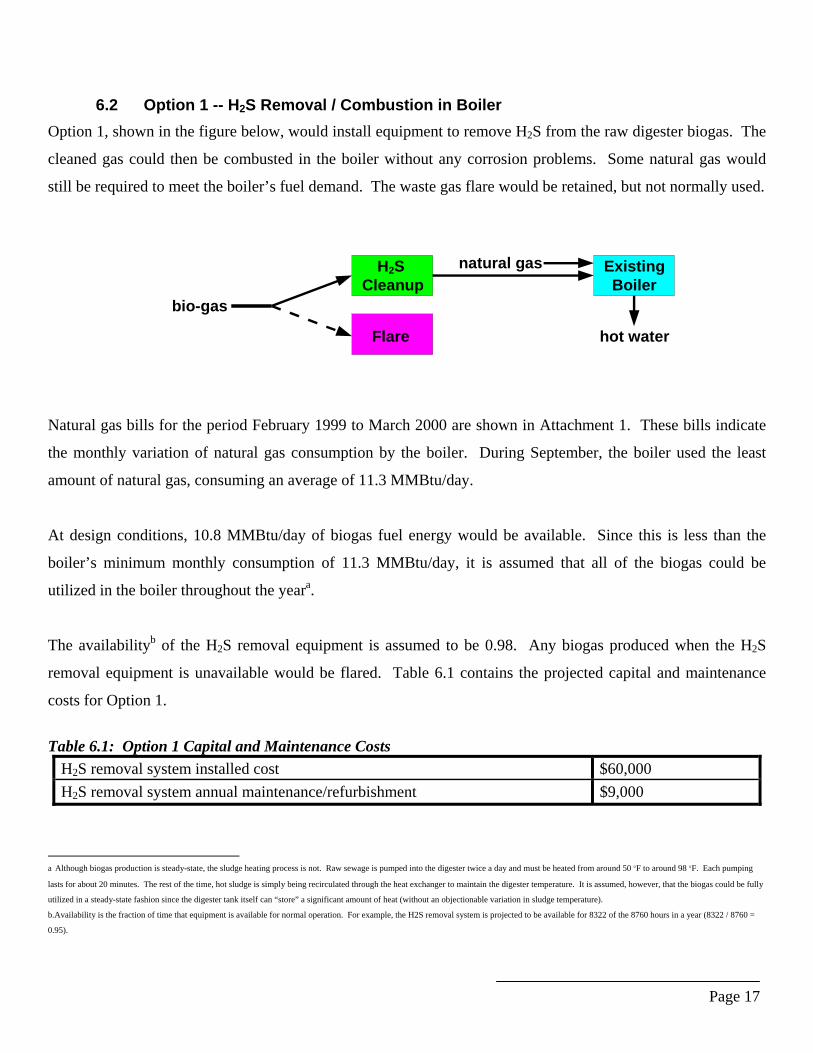
6.2 Option 1 -- H2S Removal / Combustion in Boiler Option 1, shown in the figure below, would install equipment to remove H2S from the raw digester biogas. The
cleaned gas could then be combusted in the boiler without any corrosion problems. Some natural gas would
still be required to meet the boiler’s fuel demand. The waste gas flare would be retained, but not normally used.
Natural gas bills for the period February 1999 to March 2000 are shown in Attachment 1. These bills indicate
the monthly variation of natural gas consumption by the boiler. During September, the boiler used the least
amount of natural gas, consuming an average of 11.3 MMBtu/day.
At design conditions, 10.8 MMBtu/day of biogas fuel energy would be available. Since this is less than the
boiler’s minimum monthly consumption of 11.3 MMBtu/day, it is assumed that all of the biogas could be
utilized in the boiler throughout the yeara.
The availabilityb of the H2S removal equipment is assumed to be 0.98. Any biogas produced when the H2S
removal equipment is unavailable would be flared. Table 6.1 contains the projected capital and maintenance
costs for Option 1.
Table 6.1: Option 1 Capital and Maintenance Costs
H2S removal system installed cost $60,000 H2S removal system annual maintenance/refurbishment $9,000
a Although biogas production is steady-state, the sludge heating process is not. Raw sewage is pumped into the digester twice a day and must be heated from around 50 °F to around 98 °F. Each pumping
lasts for about 20 minutes. The rest of the time, hot sludge is simply being recirculated through the heat exchanger to maintain the digester temperature. It is assumed, however, that the biogas could be fully
utilized in a steady-state fashion since the digester tank itself can “store” a significant amount of heat (without an objectionable variation in sludge temperature).
b.Availability is the fraction of time that equipment is available for normal operation. For example, the H2S removal system is projected to be available for 8322 of the 8760 hours in a year (8322 / 8760 =
0.95).
H2S Cleanup
Flare
Existing Boiler
hot water
bio-gas
natural gas
Page 18
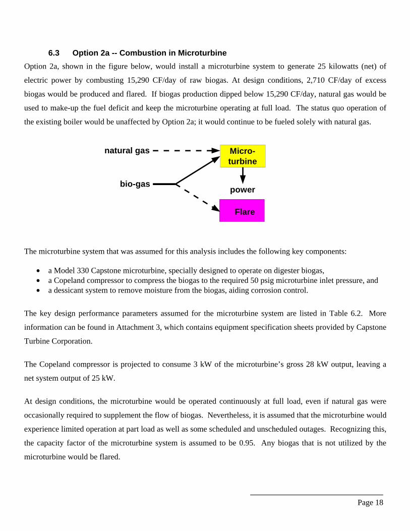
6.3 Option 2a -- Combustion in Microturbine Option 2a, shown in the figure below, would install a microturbine system to generate 25 kilowatts (net) of
electric power by combusting 15,290 CF/day of raw biogas. At design conditions, 2,710 CF/day of excess
biogas would be produced and flared. If biogas production dipped below 15,290 CF/day, natural gas would be
used to make-up the fuel deficit and keep the microturbine operating at full load. The status quo operation of
the existing boiler would be unaffected by Option 2a; it would continue to be fueled solely with natural gas.
The microturbine system that was assumed for this analysis includes the following key components:
• a Model 330 Capstone microturbine, specially designed to operate on digester biogas, • a Copeland compressor to compress the biogas to the required 50 psig microturbine inlet pressure, and • a dessicant system to remove moisture from the biogas, aiding corrosion control.
The key design performance parameters assumed for the microturbine system are listed in Table 6.2. More
information can be found in Attachment 3, which contains equipment specification sheets provided by Capstone
Turbine Corporation.
The Copeland compressor is projected to consume 3 kW of the microturbine’s gross 28 kW output, leaving a
net system output of 25 kW.
At design conditions, the microturbine would be operated continuously at full load, even if natural gas were
occasionally required to supplement the flow of biogas. Nevertheless, it is assumed that the microturbine would
experience limited operation at part load as well as some scheduled and unscheduled outages. Recognizing this,
the capacity factor of the microturbine system is assumed to be 0.95. Any biogas that is not utilized by the
microturbine would be flared.
Flare
Micro- turbine
power bio-gas
natural gas
Page 19
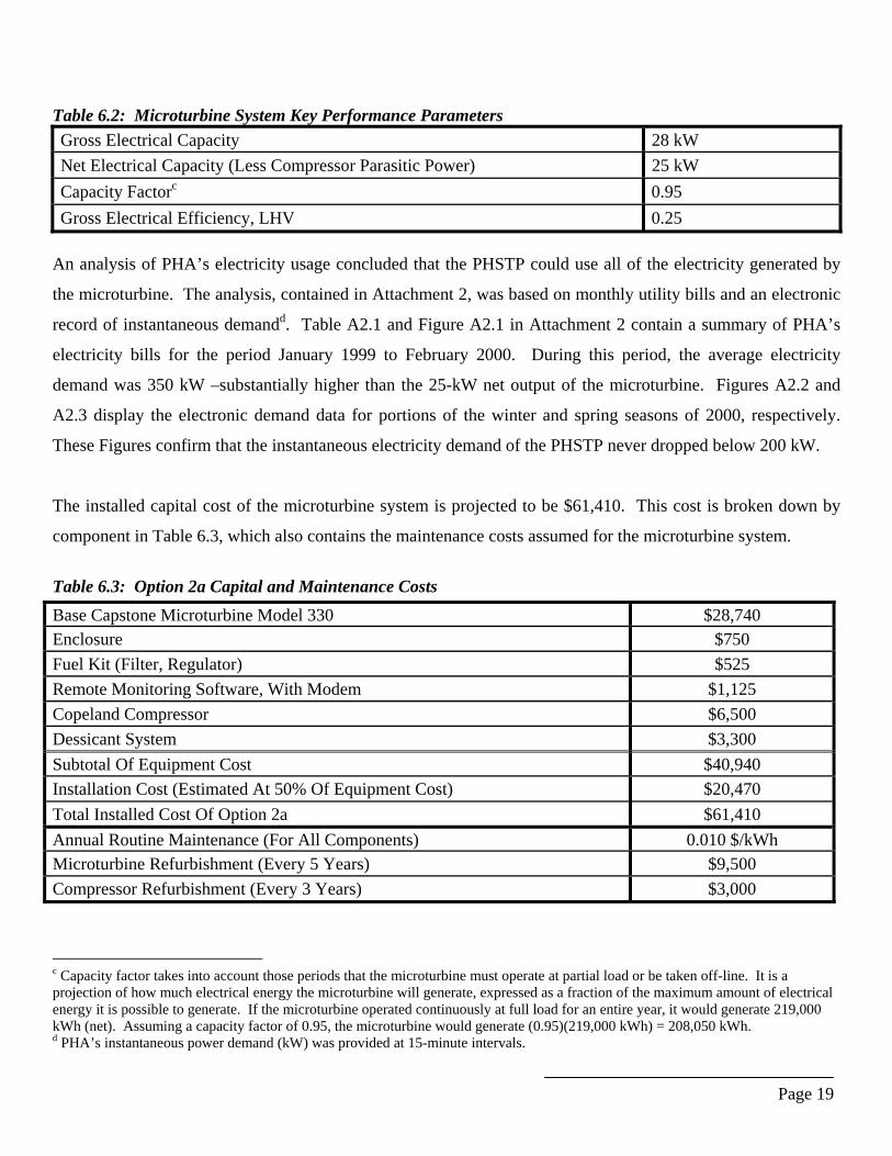
Table 6.2: Microturbine System Key Performance Parameters Gross Electrical Capacity 28 kW Net Electrical Capacity (Less Compressor Parasitic Power) 25 kW Capacity Factorc 0.95 Gross Electrical Efficiency, LHV 0.25
An analysis of PHA’s electricity usage concluded that the PHSTP could use all of the electricity generated by
the microturbine. The analysis, contained in Attachment 2, was based on monthly utility bills and an electronic
record of instantaneous demandd. Table A2.1 and Figure A2.1 in Attachment 2 contain a summary of PHA’s
electricity bills for the period January 1999 to February 2000. During this period, the average electricity
demand was 350 kW –substantially higher than the 25-kW net output of the microturbine. Figures A2.2 and
A2.3 display the electronic demand data for portions of the winter and spring seasons of 2000, respectively.
These Figures confirm that the instantaneous electricity demand of the PHSTP never dropped below 200 kW.
The installed capital cost of the microturbine system is projected to be $61,410. This cost is broken down by
component in Table 6.3, which also contains the maintenance costs assumed for the microturbine system.
Table 6.3: Option 2a Capital and Maintenance Costs
c Capacity factor takes into account those periods that the microturbine must operate at partial load or be taken off-line. It is a projection of how much electrical energy the microturbine will generate, expressed as a fraction of the maximum amount of electrical energy it is possible to generate. If the microturbine operated continuously at full load for an entire year, it would generate 219,000 kWh (net). Assuming a capacity factor of 0.95, the microturbine would generate (0.95)(219,000 kWh) = 208,050 kWh. d PHA’s instantaneous power demand (kW) was provided at 15-minute intervals.
Base Capstone Microturbine Model 330 $28,740 Enclosure $750 Fuel Kit (Filter, Regulator) $525 Remote Monitoring Software, With Modem $1,125 Copeland Compressor $6,500 Dessicant System $3,300 Subtotal Of Equipment Cost $40,940 Installation Cost (Estimated At 50% Of Equipment Cost) $20,470 Total Installed Cost Of Option 2a $61,410 Annual Routine Maintenance (For All Components) 0.010 $/kWh Microturbine Refurbishment (Every 5 Years) $9,500 Compressor Refurbishment (Every 3 Years) $3,000
Page 20
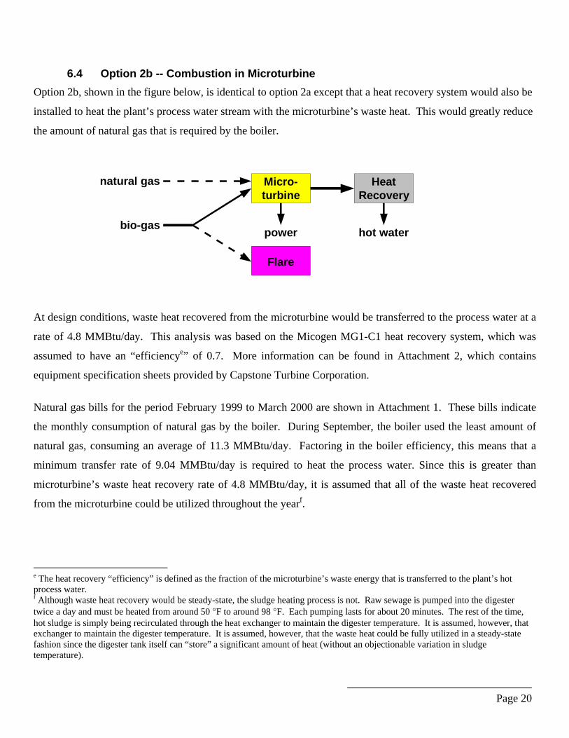
6.4 Option 2b -- Combustion in Microturbine Option 2b, shown in the figure below, is identical to option 2a except that a heat recovery system would also be
installed to heat the plant’s process water stream with the microturbine’s waste heat. This would greatly reduce
the amount of natural gas that is required by the boiler.
At design conditions, waste heat recovered from the microturbine would be transferred to the process water at a
rate of 4.8 MMBtu/day. This analysis was based on the Micogen MG1-C1 heat recovery system, which was
assumed to have an “efficiencye” of 0.7. More information can be found in Attachment 2, which contains
equipment specification sheets provided by Capstone Turbine Corporation.
Natural gas bills for the period February 1999 to March 2000 are shown in Attachment 1. These bills indicate
the monthly consumption of natural gas by the boiler. During September, the boiler used the least amount of
natural gas, consuming an average of 11.3 MMBtu/day. Factoring in the boiler efficiency, this means that a
minimum transfer rate of 9.04 MMBtu/day is required to heat the process water. Since this is greater than
microturbine’s waste heat recovery rate of 4.8 MMBtu/day, it is assumed that all of the waste heat recovered
from the microturbine could be utilized throughout the yearf.
e The heat recovery “efficiency” is defined as the fraction of the microturbine’s waste energy that is transferred to the plant’s hot process water. f Although waste heat recovery would be steady-state, the sludge heating process is not. Raw sewage is pumped into the digester twice a day and must be heated from around 50 °F to around 98 °F. Each pumping lasts for about 20 minutes. The rest of the time, hot sludge is simply being recirculated through the heat exchanger to maintain the digester temperature. It is assumed, however, that exchanger to maintain the digester temperature. It is assumed, however, that the waste heat could be fully utilized in a steady-state fashion since the digester tank itself can “store” a significant amount of heat (without an objectionable variation in sludge temperature).
Flare
Heat Recovery
hot water
Micro- turbine
power bio-gas
natural gas
Page 21
As shown by Table 6.4, the heat recovery system is estimated to add $12,642 to the installed capital cost of the
microturbine system while increasing maintenance costs by $0.001/kWh.
Table 6.4: Option 2b Capital and Maintenance Costs Micogen MG1-C1 Heat Recovery System Equipment Cost $7,224
Heat Recovery System Installation Cost (Estimated At 75% Of Equipment Cost) $5,418
Heat Recovery System Installed Cost $12,642 Microturbine System Installed Cost (From Table 6.2) $61,410 Total Installed Cost Of Option 2b $74,052 Microturbine Annual Routine Maintenance 0.010 $/kWh Heat Recovery System Annual Routine Maintenance 0.001 $/kWh Microturbine Refurbishment (Every 5 Years) $9,500 Compressor Refurbishment (Every 3 Years) $3,000
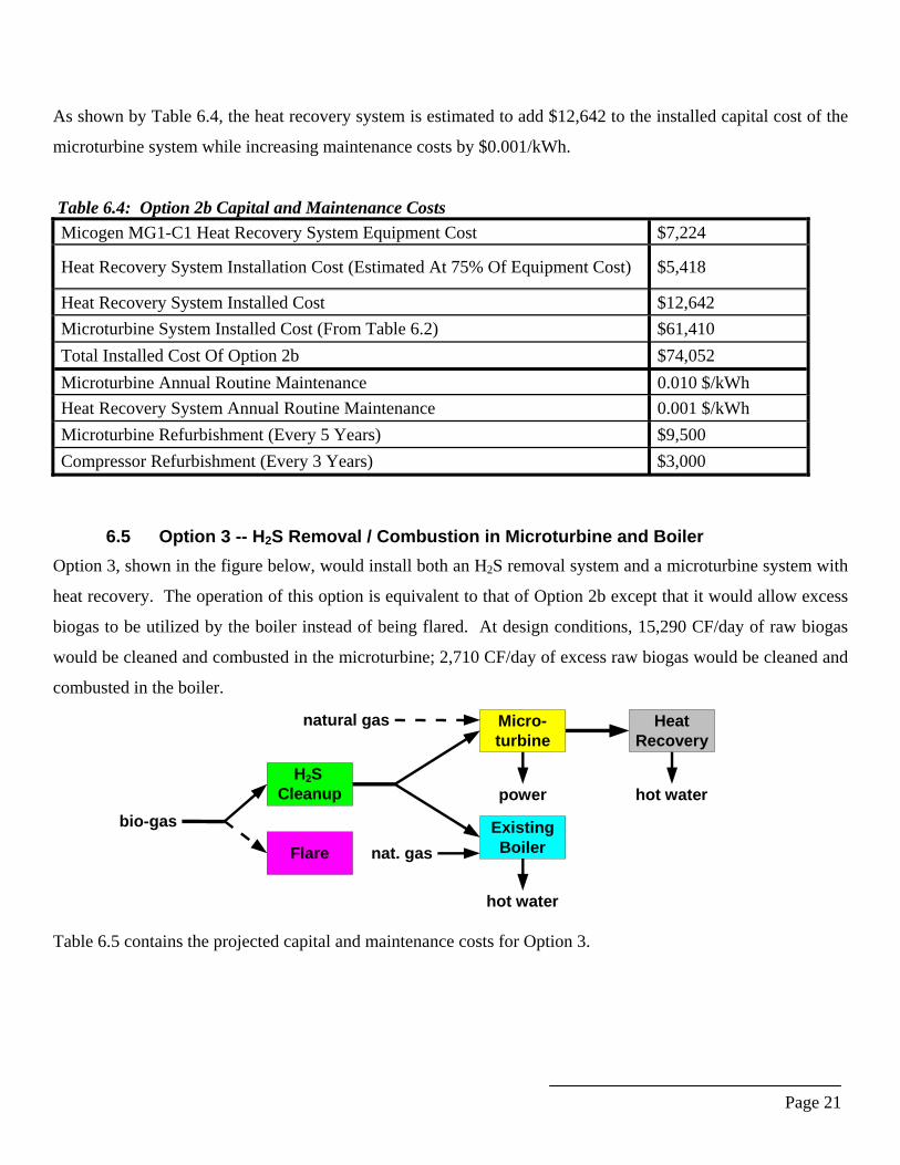
6.5 Option 3 -- H2S Removal / Combustion in Microturbine and Boiler Option 3, shown in the figure below, would install both an H2S removal system and a microturbine system with
heat recovery. The operation of this option is equivalent to that of Option 2b except that it would allow excess
biogas to be utilized by the boiler instead of being flared. At design conditions, 15,290 CF/day of raw biogas
would be cleaned and combusted in the microturbine; 2,710 CF/day of excess raw biogas would be cleaned and
combusted in the boiler.
Table 6.5 contains the projected capital and maintenance costs for Option 3.
Heat Recovery
hot water
Micro-turbine
powerbio-gas
H2S Cleanup
ExistingBoiler
hot water
Flare nat. gas
natural gas
Page 22
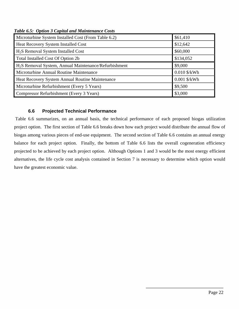
Table 6.5: Option 3 Capital and Maintenance Costs Microturbine System Installed Cost (From Table 6.2) $61,410 Heat Recovery System Installed Cost $12,642 H2S Removal System Installed Cost $60,000 Total Installed Cost Of Option 2b $134,052 H2S Removal System, Annual Maintenance/Refurbishment $9,000 Microturbine Annual Routine Maintenance 0.010 $/kWh Heat Recovery System Annual Routine Maintenance 0.001 $/kWh Microturbine Refurbishment (Every 5 Years) $9,500 Compressor Refurbishment (Every 3 Years) $3,000
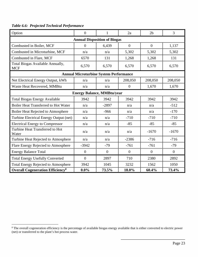
6.6 Projected Technical Performance Table 6.6 summarizes, on an annual basis, the technical performance of each proposed biogas utilization
project option. The first section of Table 6.6 breaks down how each project would distribute the annual flow of
biogas among various pieces of end-use equipment. The second section of Table 6.6 contains an annual energy
balance for each project option. Finally, the bottom of Table 6.6 lists the overall cogeneration efficiency
projected to be achieved by each project option. Although Options 1 and 3 would be the most energy efficient
alternatives, the life cycle cost analysis contained in Section 7 is necessary to determine which option would
have the greatest economic value.
Page 23
Table 6.6: Projected Technical Performance
g The overall cogeneration efficiency is the percentage of available biogas energy available that is either converted to electric power (net) or transferred to the plant’s hot process water.
Option 0 1 2a 2b 3
Annual Disposition of Biogas Combusted in Boiler, MCF 0 6,439 0 0 1,137 Combusted in Microturbine, MCF n/a n/a 5,302 5,302 5,302 Combusted in Flare, MCF 6570 131 1,268 1,268 131 Total Biogas Available Annually, MCF 6,570 6,570 6,570 6,570 6,570
Annual Microturbine System Performance Net Electrical Energy Output, kWh n/a n/a 208,050 208,050 208,050 Waste Heat Recovered, MMBtu n/a n/a 0 1,670 1,670
Energy Balance, MMBtu/year Total Biogas Energy Available 3942 3942 3942 3942 3942 Boiler Heat Transferred to Hot Water n/a -2897 n/a n/a -512 Boiler Heat Rejected to Atmosphere n/a -966 n/a n/a -170 Turbine Electrical Energy Output (net) n/a n/a -710 -710 -710 Electrical Energy to Compressor n/a n/a -85 -85 -85 Turbine Heat Transferred to Hot Water n/a n/a n/a -1670 -1670
Turbine Heat Rejected to Atmosphere n/a n/a -2386 -716 -716 Flare Energy Rejected to Atmosphere -3942 -79 -761 -761 -79 Energy Balance Total 0 0 0 0 0
Total Energy Usefully Converted 0 2897 710 2380 2892 Total Energy Rejected to Atmosphere 3942 1045 3232 1562 1050 Overall Cogeneration Efficiencyg 0.0% 73.5% 18.0% 60.4% 73.4%
Page 24
7.0 LIFE CYCLE COST ANALYSIS OF BIOGAS UTILIZATION OPTIONS In the previous section, four investment alternatives (Options 1, 2a, 2b and 3) were proposed for utilizing biogas
at the PHA wastewater treatment plant. Each alternative has a different capital cost and results in different
types and amounts of energy cost savings. Furthermore, the magnitude and timing of maintenance and
operating costs varies for each alternative. So, which of the four investments is expected to provide the greatest
return? And how does this return compare to that of other investments available to PHA? This section presents
a life cycle cost (LCC) analysis that helps to answer these questions by estimating the net present value (NPV)
of each investment alternative.
Various cash flows, such as capital costs, maintenance costs and avoided energy costs, occur at different points
throughout a project’s life. For each of the four-biogas utilization project alternatives, the timing and magnitude
of these cash flows were estimated. The cash flows were then discounted to their present values and summed to
yield a single, net present value life cycle cost estimate for each project.
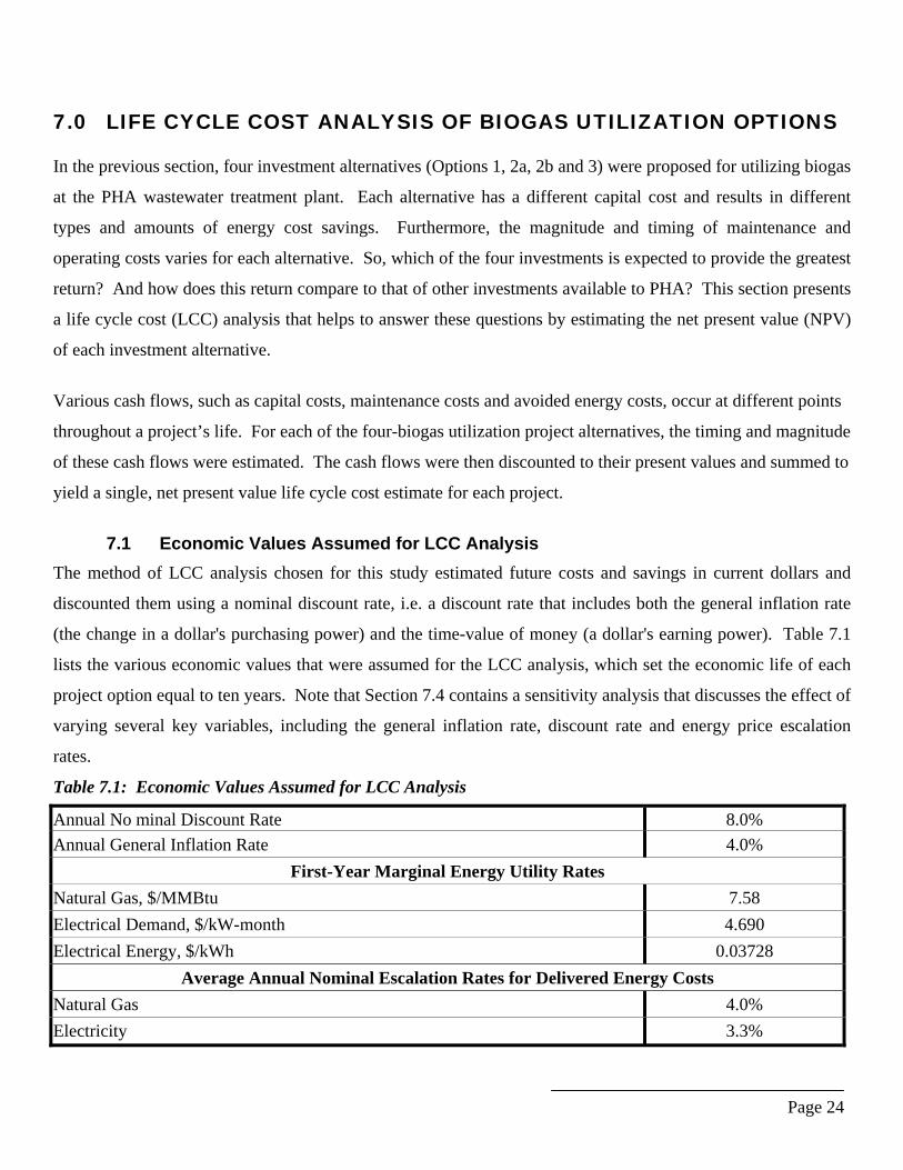
7.1 Economic Values Assumed for LCC Analysis
The method of LCC analysis chosen for this study estimated future costs and savings in current dollars and
discounted them using a nominal discount rate, i.e. a discount rate that includes both the general inflation rate
(the change in a dollar's purchasing power) and the time-value of money (a dollar's earning power). Table 7.1
lists the various economic values that were assumed for the LCC analysis, which set the economic life of each
project option equal to ten years. Note that Section 7.4 contains a sensitivity analysis that discusses the effect of
varying several key variables, including the general inflation rate, discount rate and energy price escalation
rates.
Table 7.1: Economic Values Assumed for LCC Analysis
Annual No minal Discount Rate 8.0% Annual General Inflation Rate 4.0%
First-Year Marginal Energy Utility Rates Natural Gas, $/MMBtu 7.58 Electrical Demand, $/kW-month 4.690 Electrical Energy, $/kWh 0.03728
Average Annual Nominal Escalation Rates for Delivered Energy Costs Natural Gas 4.0% Electricity 3.3%
Page 25
The annual rate of general inflation was assumed to be 4.0%. Historically, the escalation rate for construction
and maintenance costs has not deviated substantially from the general inflation rate. Therefore, maintenance
costs were assumed to escalate at the general inflation rate. On the other hand, history has also shown that
energy prices, which are much more volatile, have deviated substantially from the general inflation rateh
Therefore, the escalation rates for the prices of natural gas and electricity were considered separately.
As shown in Table A2.1 in Attachment 2, PHA’s current marginal cost of electricity has the following two
components.
• Electrical Demand: The utility measures, in kW, PHA’s peak demand for electricity during a given
billing month. Currently, the monthly marginal demand charge is $4.69 for each kW of peak demand.
• Electrical Energy: The utility measures, in kWh, how much electrical energy PHA consumes during a
given billing month. Currently, the marginal energy charge is $0.03728 for each kWh of electrical
energy consumed.
For the period 1998 to 2020, DOE’s Energy Information Administrationi projects that electricity prices for the
industrial sector will decline, in real terms, at an average annual rate of –0.7%. Assuming a general inflation
rate of 4.0%, this corresponds to a nominal annual escalation rate of 3.3%, which was applied in this analysis to
both components of PHA’s marginal electricity cost.
As shown in Attachment 1, PHA’s current marginal cost of natural gas was calculated to be $7.58/MMBtu. In
real terms, this cost was assumed to stay the same for the entire analysis period. Assuming a general inflation
rate of 4.0%, this corresponds to a nominal annual escalation rate of 4.0%.
Table 7.2 lists the marginal rates for electricity and natural gas that were calculated for each year of the LCC
analysis period.
h One advantage of using the current dollar method of LCC analysis was that it allowed energy prices to be escalated at rates different from the general rate of inflation. i See Table A3 of the Annual Energy Outlook 2000. December 1999. DOE/EIA 0383.

Page 26
Table 7.2: Utility Rates used for LCC Analysis Marginal Natural Marginal Electricity Prices
Year Gas Price, $/MCF Demand, $/kW Energy, $/kWh 1 7.58 4.690 0.037 2 7.88 4.845 0.039
3 8.20 5.005 0.040 4 8.53 5.170 0.041 5 8.87 5.340 0.042 6 9.22 5.517 0.044 7 9.59 5.699 0.045 8 9.97 5.887 0.047 9 10.37 6.081 0.048 10 10.79 6.282 0.050
The nominal annual discount rate was assumed to be 8.0% --twice that of the general inflation rate. Ideally, the
discount rate should be equivalent to the PHA’s minimum acceptable rate of return for investments of
equivalent risk and duration. In every-day business activity, nominal discount rates are usually based on market
interest rates, which include the investor's expectation of general inflation.
7.2 Life Cycle Costs
Tables 7.3 through 7.6 list the projected annual cash flows for each proposed biogas utilization project option.
Below is a description of the columns in these tables.
Year Each project alternative is assumed to have a ten-year life. Capital and Salvage Costs Installed capital costs are assigned to year one. This is due to the expectation that the design and construction
period would be brief for all project options; avoided energy costs would follow the initial capital expenditure
within a few months.
Cash flows that reflect a project’s salvage value are assigned to year ten. However, for each of the options
considered, the residual value was assumed to be equivalent to the disposal cost, i.e., the salvage value is
assumed to be zero.

Page 27
Annual Maintenance Costs Cash flows in this column reflect routine maintenance costs that occur each year. Refurbishment Costs Cash flows in this column reflect equipment refurbishment costs that are required once every few years. Avoided kWh Costs Cash flows in this column reflect the portion of avoided electric utility costs that result from a reduced
consumption of utility-provided electrical energy (kWh). The reduction is equal to the net amount of electrical
energy that would be generated by the microturbine for the PHSTP.
Avoided kW Costs Cash flows in this column reflect the portion of avoided electric utility costs that result from a reduced peak
demand (kW) for utility-provided electricity. The total demand charge that is avoided in one year is calculated
by summing the twelve monthly reductions in peak demand that are obtained by operating the microturbine. At
design conditions, the microturbine would continuously generate 25 kW (net), resulting in a 25 kW reduction in
monthly peak demand. However, in a given year there could be months during which the microturbine operates
at part-load for a few hours, and months during which it would experience a complete outage. Therefore, for
the purpose of calculating the annual avoided electricity demand costs, the following (conservative)
assumptions were made.
For eight months each year, the microturbine would continuously generate 25 kW (net), reducing peak demand
by 25 kW.
For brief periods during two months each year, the microturbine would be operated at part-load, resulting in a
peak demand reduction of only 12.5 kW.
For a few days during two months each year, the microturbine would be taken out of service, resulting in no
reduction in peak demand.
This analysis assumed that the electric utility would not charge PHA with a fee for the service of standing by to
provide 25 kW of back-up power in the event the microturbine becomes unavailable. If assessed, such a fee
could have a significant adverse impact on project economics.
Page 28
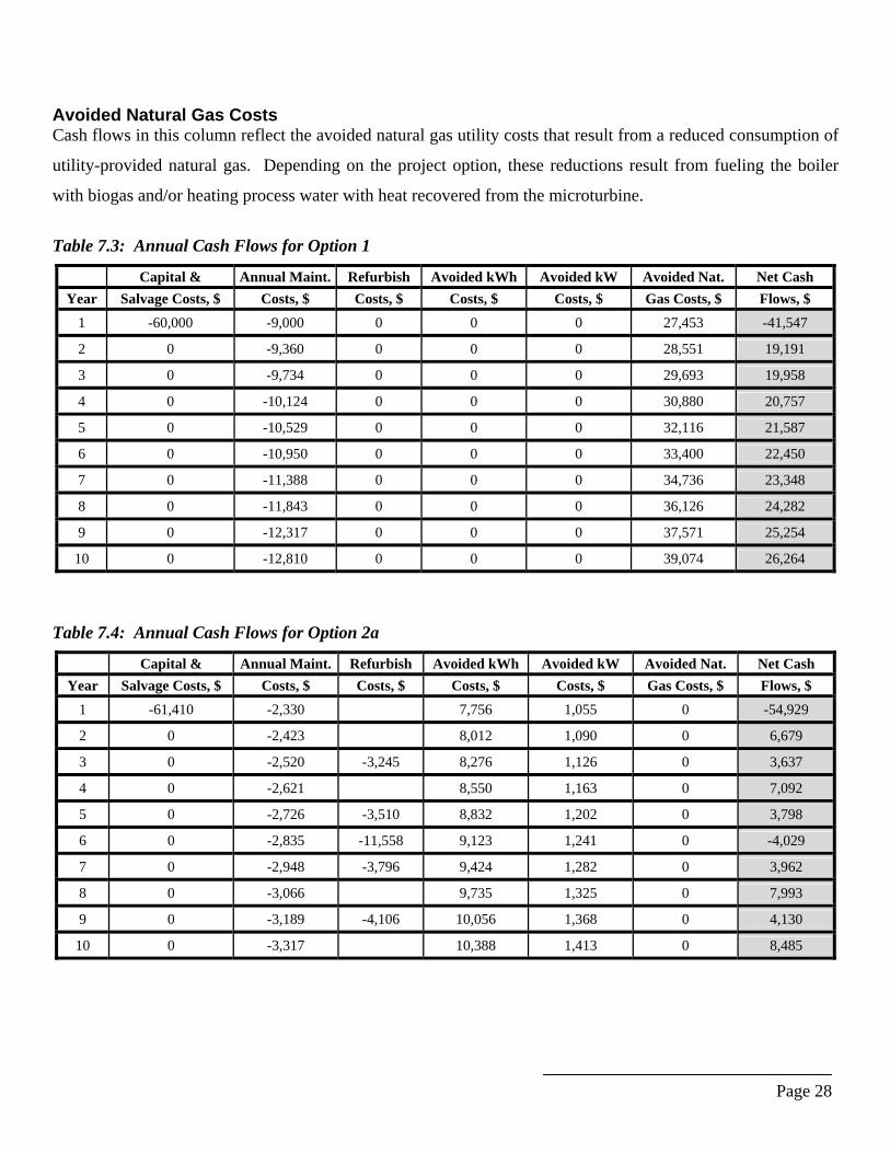
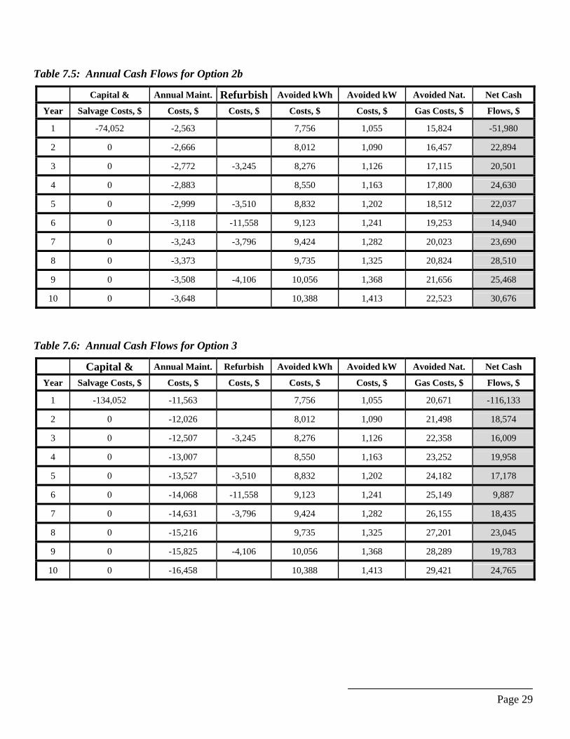
Avoided Natural Gas Costs Cash flows in this column reflect the avoided natural gas utility costs that result from a reduced consumption of
utility-provided natural gas. Depending on the project option, these reductions result from fueling the boiler
with biogas and/or heating process water with heat recovered from the microturbine. Table 7.3: Annual Cash Flows for Option 1
Capital & Annual Maint. Refurbish Avoided kWh Avoided kW Avoided Nat. Net Cash Year Salvage Costs, $ Costs, $ Costs, $ Costs, $ Costs, $ Gas Costs, $ Flows, $
1 -60,000 -9,000 0 0 0 27,453 -41,547
2 0 -9,360 0 0 0 28,551 19,191
3 0 -9,734 0 0 0 29,693 19,958
4 0 -10,124 0 0 0 30,880 20,757
5 0 -10,529 0 0 0 32,116 21,587
6 0 -10,950 0 0 0 33,400 22,450
7 0 -11,388 0 0 0 34,736 23,348
8 0 -11,843 0 0 0 36,126 24,282
9 0 -12,317 0 0 0 37,571 25,254
10 0 -12,810 0 0 0 39,074 26,264
Table 7.4: Annual Cash Flows for Option 2a
Capital & Annual Maint. Refurbish Avoided kWh Avoided kW Avoided Nat. Net Cash Year Salvage Costs, $ Costs, $ Costs, $ Costs, $ Costs, $ Gas Costs, $ Flows, $
1 -61,410 -2,330 7,756 1,055 0 -54,929
2 0 -2,423 8,012 1,090 0 6,679
3 0 -2,520 -3,245 8,276 1,126 0 3,637
4 0 -2,621 8,550 1,163 0 7,092
5 0 -2,726 -3,510 8,832 1,202 0 3,798
6 0 -2,835 -11,558 9,123 1,241 0 -4,029
7 0 -2,948 -3,796 9,424 1,282 0 3,962
8 0 -3,066 9,735 1,325 0 7,993
9 0 -3,189 -4,106 10,056 1,368 0 4,130
10 0 -3,317 10,388 1,413 0 8,485
Page 29
Table 7.5: Annual Cash Flows for Option 2b
Capital & Annual Maint. Refurbish Avoided kWh Avoided kW Avoided Nat. Net Cash
Year Salvage Costs, $ Costs, $ Costs, $ Costs, $ Costs, $ Gas Costs, $ Flows, $
1 -74,052 -2,563 7,756 1,055 15,824 -51,980
2 0 -2,666 8,012 1,090 16,457 22,894
3 0 -2,772 -3,245 8,276 1,126 17,115 20,501
4 0 -2,883 8,550 1,163 17,800 24,630
5 0 -2,999 -3,510 8,832 1,202 18,512 22,037
6 0 -3,118 -11,558 9,123 1,241 19,253 14,940
7 0 -3,243 -3,796 9,424 1,282 20,023 23,690
8 0 -3,373 9,735 1,325 20,824 28,510
9 0 -3,508 -4,106 10,056 1,368 21,656 25,468
10 0 -3,648 10,388 1,413 22,523 30,676
Table 7.6: Annual Cash Flows for Option 3
Capital & Annual Maint. Refurbish Avoided kWh Avoided kW Avoided Nat. Net Cash
Year Salvage Costs, $ Costs, $ Costs, $ Costs, $ Costs, $ Gas Costs, $ Flows, $
1 -134,052 -11,563 7,756 1,055 20,671 -116,133
2 0 -12,026 8,012 1,090 21,498 18,574
3 0 -12,507 -3,245 8,276 1,126 22,358 16,009
4 0 -13,007 8,550 1,163 23,252 19,958
5 0 -13,527 -3,510 8,832 1,202 24,182 17,178
6 0 -14,068 -11,558 9,123 1,241 25,149 9,887
7 0 -14,631 -3,796 9,424 1,282 26,155 18,435
8 0 -15,216 9,735 1,325 27,201 23,045
9 0 -15,825 -4,106 10,056 1,368 28,289 19,783
10 0 -16,458 10,388 1,413 29,421 24,765
Page 30
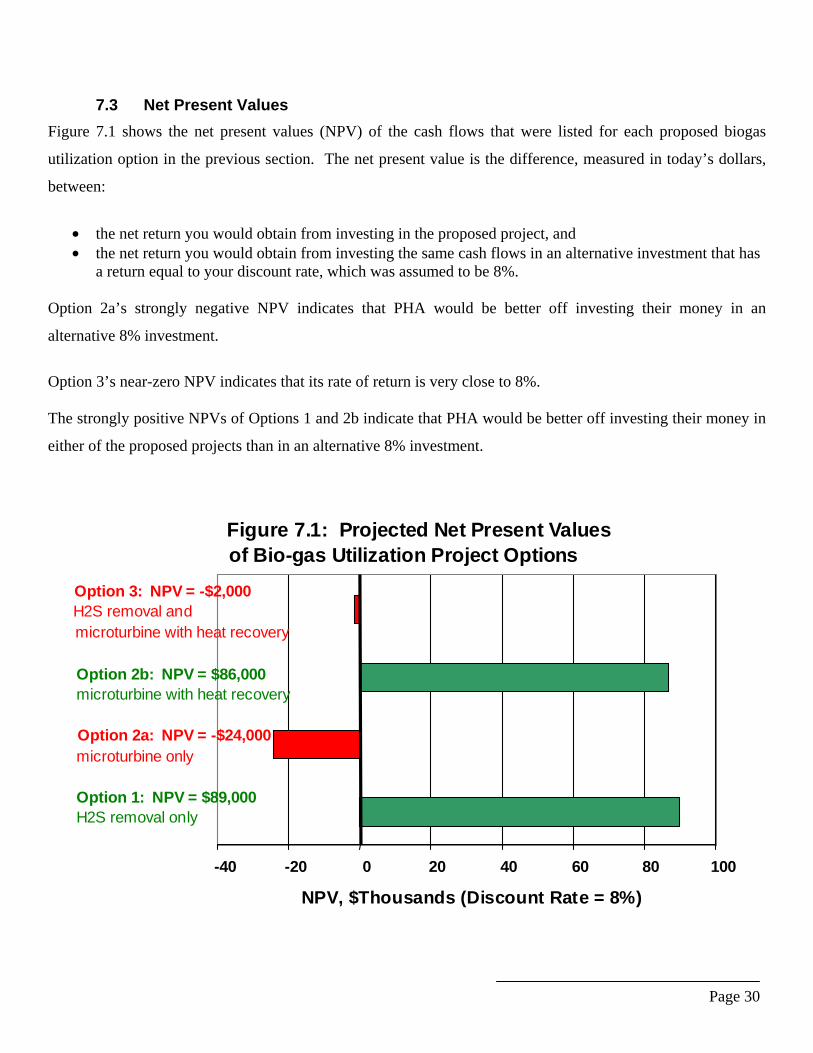
7.3 Net Present Values Figure 7.1 shows the net present values (NPV) of the cash flows that were listed for each proposed biogas
utilization option in the previous section. The net present value is the difference, measured in today’s dollars,
between:
• the net return you would obtain from investing in the proposed project, and • the net return you would obtain from investing the same cash flows in an alternative investment that has
a return equal to your discount rate, which was assumed to be 8%. Option 2a’s strongly negative NPV indicates that PHA would be better off investing their money in an
alternative 8% investment.
Option 3’s near-zero NPV indicates that its rate of return is very close to 8%. The strongly positive NPVs of Options 1 and 2b indicate that PHA would be better off investing their money in
either of the proposed projects than in an alternative 8% investment.
Figure 7.1: Projected Net Present Values of Bio-gas Utilization Project Options
-40 -20 0 20 40 60 80 100
NPV, $Thousands (Discount Rate = 8%)
Option 3: NPV = -$2,000 H2S removal and microturbine with heat recovery
Option 2b: NPV = $86,000 microturbine with heat recovery
Option 2a: NPV = -$24,000 microturbine only
Option 1: NPV = $89,000 H2S removal only
Page 31
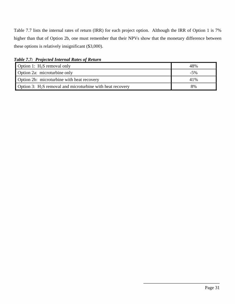
Table 7.7 lists the internal rates of return (IRR) for each project option. Although the IRR of Option 1 is 7%
higher than that of Option 2b, one must remember that their NPVs show that the monetary difference between
these options is relatively insignificant ($3,000).
Table 7.7: Projected Internal Rates of Return
Option 1: H2S removal only 48% Option 2a: microturbine only -5% Option 2b: microturbine with heat recovery 41% Option 3: H2S removal and microturbine with heat recovery 8%

Page 32
7.4 Sensitivity Analyses
The above LCC analysis indicates that Options 1 and 2b would be the most economically attractive of the
proposed biogas utilization projects. Therefore, these two options were selected for a sensitivity analysis to
determine the effect of varying the assumed values of key economic and technical variables.
Sensitivity of Discount and Inflation Rates Figures 7.2 and 7.3 show the effect on project NPV of varying the discount and inflation rates. The NPVs of Options 1 and 2 would remain positive for a wide range of credible discount rates. Relative to the discount rate, the inflation rate would have a weak effect on NPV.
Figure 7.2: Sensitivity of Discount and Inflation RatesCase 1: H2S Removal; Combustion in Boiler
0
20,000
40,000
60,000
80,000
100,000
120,000
0 0.1 0.2 0.3 0.4 0.5Nominal Discount Rate
NPV
0.00.00.00.1
General Inflation Rates
Figure 7.3: Sensitivity of Discount and Inflation RatesCase 2b: Microturbine with Heat Recovery
0
20,000
40,000
60,000
80,000
100,000
120,000
0 0.1 0.2 0.3 0.4 0.5Nominal Discount Rate
NPV
0.00.00.00.1
General Inflation Rates
Page 33
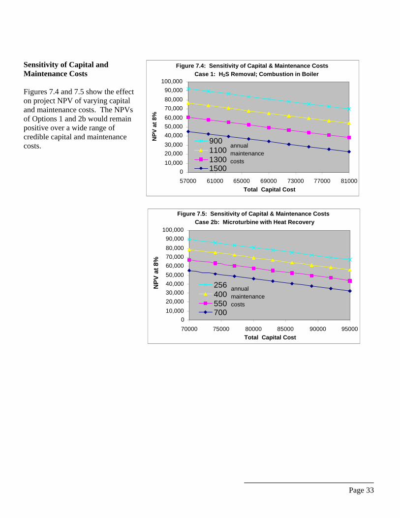
Sensitivity of Capital and Maintenance Costs Figures 7.4 and 7.5 show the effect on project NPV of varying capital and maintenance costs. The NPVs of Options 1 and 2b would remain positive over a wide range of credible capital and maintenance costs.
Figure 7.4: Sensitivity of Capital & Maintenance Costs Case 1: H2S Removal; Combustion in Boiler
010,00020,00030,00040,00050,00060,00070,00080,00090,000
100,000
57000 61000 65000 69000 73000 77000 81000Total Capital Cost
NPV
at 8
%
900110013001500
annualmaintenancecosts
Figure 7.5: Sensitivity of Capital & Maintenance Costs Case 2b: Microturbine with Heat Recovery
010,00020,00030,00040,00050,00060,00070,00080,00090,000
100,000
70000 75000 80000 85000 90000 95000Total Capital Cost
NPV
at 8
%
256400550700
annualmaintenancecosts
Page 34
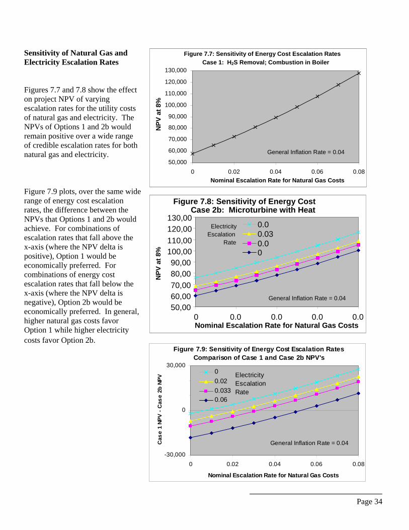
Sensitivity of Natural Gas and Electricity Escalation Rates Figures 7.7 and 7.8 show the effect on project NPV of varying escalation rates for the utility costs of natural gas and electricity. The NPVs of Options 1 and 2b would remain positive over a wide range of credible escalation rates for both natural gas and electricity. Figure 7.9 plots, over the same wide range of energy cost escalation rates, the difference between the NPVs that Options 1 and 2b would achieve. For combinations of escalation rates that fall above the x-axis (where the NPV delta is positive), Option 1 would be economically preferred. For combinations of energy cost escalation rates that fall below the x-axis (where the NPV delta is negative), Option 2b would be economically preferred. In general, higher natural gas costs favor Option 1 while higher electricity costs favor Option 2b.
Figure 7.9: Sensitivity of Energy Cost Escalation RatesComparison of Case 1 and Case 2b NPV's
-30,000
0
30,000
0 0.02 0.04 0.06 0.08
Nominal Escalation Rate for Natural Gas Costs
Cas
e 1
NPV
- C
ase
2b N
PV
00.020.0330.06
ElectricityEscalationRate
General Inflation Rate = 0.04
Figure 7.7: Sensitivity of Energy Cost Escalation Rates Case 1: H2S Removal; Combustion in Boiler
50,000
60,000
70,000
80,000
90,000
100,000
110,000
120,000
130,000
0 0.02 0.04 0.06 0.08Nominal Escalation Rate for Natural Gas Costs
NPV
at 8
%
General Inflation Rate = 0.04
Figure 7.8: Sensitivity of Energy Cost Case 2b: Microturbine with Heat
50,0060,0070,0080,0090,00
100,00110,00120,00130,00
0 0.0 0.0 0.0 0.0Nominal Escalation Rate for Natural Gas Costs
NPV
at 8
%
0.00.030.00
Electricity Escalation
Rate
General Inflation Rate = 0.04

Page 35
Sensitivity of Biogas Production Rate and Heating Value Figures 7.10 and 7.11 show the effect on project NPV of varying the biogas production rate and heating value. The NPVs of Options 1 and 2b would remain positive over a wide range of credible biogas production rates and heating values. As the assumed value for biogas production is increased, the NPV of Option 2b is limited by the fact that only one microturbine is included in the system. If biogas production dramatically increased, more microturbines could be installed to utilize it. Sensitivity of Microturbine Capacity Factor and Heat Recovery Efficiency Figure 7.12 shows the effect on project NPV of varying the microturbine’s capacity factor and the heat recovery system’s “efficiency.” The NPV of Option 2b would remain positive over a wide range of credible values for microturbine capacity factor and heat recovery system efficiency. (These technical parameters are not applicable to Option 1.)
Figure 7.12: Sensitivity of Turbine Capacity Factor & HR EffCase 2b: Microturbine with Heat Recovery
0
20,000
40,000
60,000
80,000
100,000
120,000
0.91 0.92 0.93 0.94 0.95 0.96 0.97 0.98 0.99Microturbine System Capacity Factor
NPV
at 8
%
0.80.70.60.5
heatrecovery
efficiency
Figure 7.10: Sensitivity of Biogas Production & Heat ValueCase 1: H2S Removal; Combustion in B il
0
20,000
40,000
60,000
80,000
100,000
120,000
140,000
160,000
14000 16000 18000 20000 22000Bio-Gas Production, CF/d
NPV
at 8
%
650600550500
Bio-Gas Lower Heating Value, Btu/CF
Figure 7.11: Sensitivity of Biogas Production & Heat ValueCase 2b: Microturbine with Heat Recovery
0
20,000
40,000
60,000
80,000
100,000
120,000
140,000
160,000
14000 16000 18000 20000 22000Bio-Gas Production, CF/d
NPV
at 8
%
650600550500
Bio-Gas Lower Heating Value, Btu/CF

Page 36
8.0 CLIMATE CHANGE AND EMISSIONS The current PHSTP emissions are comprised of greenhouse gas and criteria pollutants. Criteria pollutants,
sulfur dioxide (SO2) and nitrous oxide (NOX) affect smog development, while greenhouse gases are cited as a
major source of global warming.
Local Climate Change Criteria pollutants cause ground level development of ozone; ground-level ozone is also known as smog. The
1990 Clean Air Act regulates both particulate and criteria pollutant emissions, which bring about ground level
pollution. While the 1990 Act primarily addresses large stationary sources mobile sources, it also concerns a
variety of sources and mitigation strategies. As ground level pollution levels worsen, pollution controls may be
required for smaller stationary sources.
Global Climate Change Concern for the potential effect of anthropogenic emissions upon global climate has led to the U.S. agreement
in Kyoto to a 7% decrease in greenhouse gas (GHG) emission between 2008 and 2012, based on 1990 levels,
which must still be ratified by the U.S. Senate26. Carbon and other GHG emissions are not yet regulated; the
most populous carbon compounds in U.S. emissions are carbon dioxide, CO2, and methane, CH4. Carbon
dioxide is the most prevalent GHG and has a considerably longer lifetime than methane. The compounds exist
in the atmosphere for 50-200 years and 12 years, respectively. However, methane emissions are of great
concern because it has 21 times the ability of carbon dioxide to trap heat in the atmosphere. Furthermore, it is
possible to accurately measure carbon dioxide emissions within 3-5% because sources of carbon dioxide are
easily isolated7, 14.
However, accurate measurement of methane source emissions is not easily achieved, although they are believed
to account for 10% of U.S. GHG emissions7, 19. Most methane is emitted accidentally or occurs naturally as a
byproduct of farming and therefore is not easily measured. About 95% of the methane in the U.S. is emitted in
large quantities from landfills, livestock management, natural gas systems, coal mining, and manure
management. Smaller sources include rice farming, wastewater treatment, and biomass burning, all of which
account for less than 1.5% of the total methane emitted nationally14,19.
GHG Emissions and Reductions Data for U.S. The Energy Policy Act of 1992 requires the Energy Information Administration (EIA) to prepare a report on
aggregate U.S. national emissions of greenhouses gases for the period 1987-1990, with annual updates
Page 37
thereafter8. The EIA report presents estimates of U.S. anthropogenic emissions of carbon dioxide, methane,
nitrous oxide, halocarbons and criteria pollutants. Industrial wastewater treatment is not addressed in this
survey because it is believed that methane emissions from industrial wastewater treatment are a byproduct of
the method used to treat wastewater. Due to limited data available regarding wastewater treatment methods or
the amount of water treated, it is not possible to present estimates of methane emissions from industrial
wastewater9.
The EIA has a voluntary program that records the results of voluntary measures taken to reduce, avoid, or
sequester greenhouse gas emissions (Section 1605(b) of the Energy Policy Act of 1992). In 1994, the first year
of the program, 108 facilities reported aggregate reductions of 74 million tons carbon equivalent (mtce). In
1998, 187 facilities reported 212 mtce10. Several participants have perceived EIA’s Voluntary Reporting
Program as a method to achieving regulatory credit10. However, this program is designed to be a registry of
reduction levels achieved, not provide and arena for emissions trading or to provide credit for early reductions.
One wastewater treatment entity, the City of Fairfield Wastewater Division in Ohio, reported reduction of
emissions during 1998. The method of reducing greenhouse emissions for this facility was to recover biogas for
energy use, thus reducing carbon dioxide emissions by 631 metric tce, and no changes in methane emissions11.
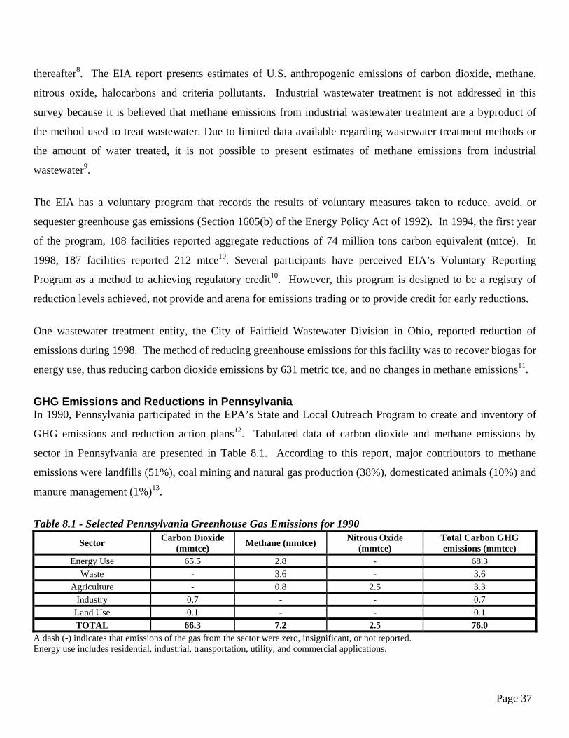
GHG Emissions and Reductions in Pennsylvania In 1990, Pennsylvania participated in the EPA’s State and Local Outreach Program to create and inventory of
GHG emissions and reduction action plans12. Tabulated data of carbon dioxide and methane emissions by
sector in Pennsylvania are presented in Table 8.1. According to this report, major contributors to methane
emissions were landfills (51%), coal mining and natural gas production (38%), domesticated animals (10%) and
manure management (1%)13.
Table 8.1 - Selected Pennsylvania Greenhouse Gas Emissions for 1990
Sector Carbon Dioxide (mmtce) Methane (mmtce) Nitrous Oxide
(mmtce) Total Carbon GHG emissions (mmtce)
Energy Use 65.5 2.8 - 68.3 Waste - 3.6 - 3.6
Agriculture - 0.8 2.5 3.3 Industry 0.7 - - 0.7
Land Use 0.1 - - 0.1 TOTAL 66.3 7.2 2.5 76.0
A dash (-) indicates that emissions of the gas from the sector were zero, insignificant, or not reported. Energy use includes residential, industrial, transportation, utility, and commercial applications.

Page 38
Pleasant Hills Case Overview Although wastewater treatment is not identified as a significant source of methane, opportunities to mitigate
methane should be not overlooked if the cost of reduction is affordable. There are also local benefits to be
gained from lowering GHG emission levels. To date, Pleasant Hills Authority has estimated that methane
comprises 68% of the fugitive gas from their sewage treatment plant that treats wastewater for approximately
12,000 households for the Pleasant Hills borough of Pittsburgh, PA. The potential for biogas collection will be
quantified and analyzed to determine the feasible level of GHG mitigation and resources for energy production
application.
This preliminary case study is the result of a feasibility team investigation of alternatives to reduce GHG
emissions at the Pleasant Hills wastewater treatment plant. The benefits of Pleasant Hills Authority
participation in a pilot GHG reduction project with NETL are two-fold. The Authority obtains retrofit
technology that may result in economic gain and serve as a prototype for other such projects for municipal
sewage treatment plants across the country. Retrofitting the current process to collect methane may collect a
sufficient amount of gas for power generation, so that the facility may provide energy for in-house use, or sale
to the utility distribution. Ancillary benefits from collecting methane gas include a decrease in “stink” from
hydrogen sulfide and decreases in carbon dioxide emissions19 as well as a decrease in criteria pollutant
emission4.
Currently, nitrous oxide, methane, and carbon dioxide are the main constituents of GHG emissions from the
Pleasant Hills facility, as will be discussed in the Section 9.0, “Emissions from Alternate Options”. Many
methods of decreasing methane emissions similarly decrease carbon dioxide emissions19. Nitrous oxide is of
particular concern; although it comprises an insignificant percentage of wastewater treatment emissions, it has
300 times the global warming potential of carbon dioxide8. As mentioned before, hydrogen sulfide is not a
greenhouse gas, but may play a future role in health concerns, since sulfur oxides, criteria pollutants regulated
by the Clean Air Act, result from combustion of hydrogen sulfide. Additionally, analysis of hydrogen sulfide
concentrations in sewage air have reported in literature of correlation between hydrogen sulfide concentration
and unpleasant, “rotten egg”, odor in the air surrounding a treatment facility20. Determined to be an irritant to
mucous membranes and a potential carcinogen by the EPA National Center for Environmental Assessment,
hydrogen sulfide is being considered for listing as a hazardous air pollutant (HAP) as defined under the Clean
Air Act11.
Page 39
9.0 EMISSIONS FROM ALTERNATE PROCESS OPTIONS The following is an estimation of potential emissions that may be expected from the installation of each
proposed case as described in Section 6. Estimations of current pollutant emissions, Case 0, are summarized
from the existing system involving flared biogas and natural gas boiler use, then compared to potential
emissions from Cases 1, 2a, 2b, and 3 to determine potential change in emissions. Estimates are based on
current digester gas composition and microturbine operations data. Combustion coefficients and calculations are
adapted from Steam, its generation and use, 40th ed., by Babcock and Wilcox Company1.
In order to estimate the potential for GHG emission reduction, emissions levels are converted to their metric ton
carbon equivalent (mtce) by a factor of their relative global warming potential. After determining their carbon
equivalence, their potential economic value may be determined by a factor of the cost of avoided health and
environmental damages21; approximately $14 per mtce. This value is well below the EIA’s estimated tax of
$348 per mtce required to achieve Kyoto budgets in 2010 without global GHG credit trading4. Global warming
potential factors are a means of determining the ability of GHG to trap heat in the atmosphere. It has been
determined that the global warming potentials of methane, nitrous oxide and nitrogen oxide are 21, 310 and 290
times that of carbon dioxide18, 17, respectively.
Of additional importance is criteria pollutant reduction through technology installation. Sulfur oxide (SOX), and
nitrous oxide (NOX) emissions are regulated by the Clean Air Act. Criteria pollutant reductions are valuable,
since they may be traded and sold as a commodity; trading options will be discussed further in Section 9.3,
“Determining Potential Economic Value of Emissions Reduction”.
Overview of Available Biogas and Natural Gas Biogas Composition Current estimates of digester biogas flow, 18,000 cfd, heat value, 600 BTU/cf, and measured composition
(Table 3.1) for the PHSTP were used to analyze greenhouse gas emissions under current conditions and
possible alternatives for reducing emissions.
Note that oxygen and nitrogen are present at the same ratio as that for air, which suggests that some air leaked into the sample. Using current biogas data, the molar composition of 100 lbs of biogas to be used in combustion may be stoichiometrically determined, and consequently used to determine emissions. The molar
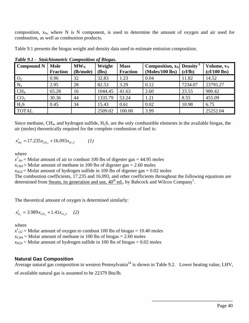
Page 40
composition, xN, where N is N component, is used to determine the amount of oxygen and air used for combustion, as well as combustion products. Table 9.1 presents the biogas weight and density data used to estimate emission composition. Table 9.1 - Stoichiometric Composition of Biogas. Compound N Mole
Fraction MWN (lb/mole)
Weight (lbs)
Mass Fraction
Composition, xN (Moles/100 lbs)
Density-1 (cf/lb)
Volume, vN (cf/100 lbs)
O2 0.96 32 32.83 1.23 0.04 11.82 14.52 N2 2.95 28 82.53 3.29 0.12 7234.07 23795.27 CH4 65.28 16 1044.45 41.63 2.60 23.55 980.42 CO2 30.36 44 1335.79 53.24 1.21 8.55 455.09 H2S 0.45 34 15.43 0.61 0.02 10.98 6.75 TOTAL 2509.02 100.00 3.99 25252.04
Since methane, CH4, and hydrogen sulfide, H2S, are the only combustible elements in the available biogas, the air (moles) theoretically required for the complete combustion of fuel is:
SHCHAir xxx24
093.16235.171 += (1) where x1
Air = Molar amount of air to combust 100 lbs of digester gas = 44.95 moles xCH4 = Molar amount of methane in 100 lbs of digester gas = 2.60 moles xH2S = Molar amount of hydrogen sulfide in 100 lbs of digester gas = 0.02 moles The combustion coefficients, 17.235 and 16.093, and other coefficients throughout the following equations are determined from Steam, its generation and use, 40th ed., by Babcock and Wilcox Company1.
The theoretical amount of oxygen is determined similarly:
SHCHO xxx242
41.1989.31 += (2) where x1
O2 = Molar amount of oxygen to combust 100 lbs of biogas = 10.40 moles xCH4 = Molar amount of methane in 100 lbs of biogas = 2.60 moles xH2S = Molar amount of hydrogen sulfide in 100 lbs of biogas = 0.02 moles Natural Gas Composition Average natural gas composition in western Pennsylvania24 is shown in Table 9.2. Lower heating value, LHV,
of available natural gas is assumed to be 22379 Btu/lb.
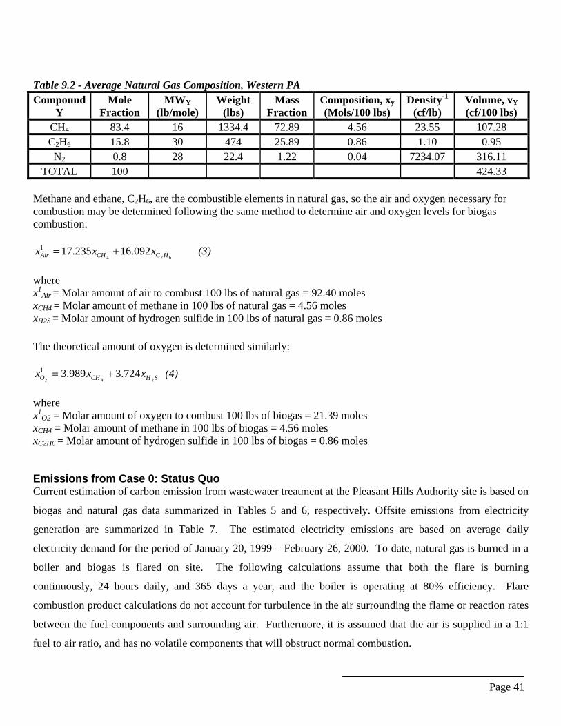
Page 41
Table 9.2 - Average Natural Gas Composition, Western PA Compound
Y Mole
Fraction MWY
(lb/mole) Weight
(lbs) Mass
Fraction Composition, xy (Mols/100 lbs)
Density-1 (cf/lb)
Volume, vY (cf/100 lbs)
CH4 83.4 16 1334.4 72.89 4.56 23.55 107.28 C2H6 15.8 30 474 25.89 0.86 1.10 0.95 N2 0.8 28 22.4 1.22 0.04 7234.07 316.11
TOTAL 100 424.33 Methane and ethane, C2H6, are the combustible elements in natural gas, so the air and oxygen necessary for combustion may be determined following the same method to determine air and oxygen levels for biogas combustion:
624092.16235.171
HCCHAir xxx += (3) where x1
Air = Molar amount of air to combust 100 lbs of natural gas = 92.40 moles xCH4 = Molar amount of methane in 100 lbs of natural gas = 4.56 moles xH2S = Molar amount of hydrogen sulfide in 100 lbs of natural gas = 0.86 moles
The theoretical amount of oxygen is determined similarly:
SHCHO xxx242
724.3989.31 += (4) where x1
O2 = Molar amount of oxygen to combust 100 lbs of biogas = 21.39 moles xCH4 = Molar amount of methane in 100 lbs of biogas = 4.56 moles xC2H6 = Molar amount of hydrogen sulfide in 100 lbs of biogas = 0.86 moles Emissions from Case 0: Status Quo Current estimation of carbon emission from wastewater treatment at the Pleasant Hills Authority site is based on
biogas and natural gas data summarized in Tables 5 and 6, respectively. Offsite emissions from electricity
generation are summarized in Table 7. The estimated electricity emissions are based on average daily
electricity demand for the period of January 20, 1999 – February 26, 2000. To date, natural gas is burned in a
boiler and biogas is flared on site. The following calculations assume that both the flare is burning
continuously, 24 hours daily, and 365 days a year, and the boiler is operating at 80% efficiency. Flare
combustion product calculations do not account for turbulence in the air surrounding the flame or reaction rates
between the fuel components and surrounding air. Furthermore, it is assumed that the air is supplied in a 1:1
fuel to air ratio, and has no volatile components that will obstruct normal combustion.
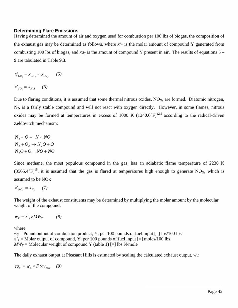
Page 42
Determining Flare Emissions Having determined the amount of air and oxygen used for combustion per 100 lbs of biogas, the composition of
the exhaust gas may be determined as follows, where x’Y is the molar amount of compound Y generated from
combusting 100 lbs of biogas, and xaY is the amount of compound Y present in air. The results of equations 5 –
9 are tabulated in Table 9.3.
242
' COCHCO xxx += (5)
SHSO xx22
' = (6) Due to flaring conditions, it is assumed that some thermal nitrous oxides, NOX, are formed. Diatomic nitrogen,
N2, is a fairly stable compound and will not react with oxygen directly. However, in some flames, nitrous
oxides may be formed at temperatures in excess of 1000 K (1340.6°F)1,15 according to the radical-driven
Zeldovitch mechanism:
NONOOONOONON
NONON
+=++→+
+→+
2
222
2
Since methane, the most populous compound in the gas, has an adiabatic flame temperature of 2236 K
(3565.4°F)15, it is assumed that the gas is flared at temperatures high enough to generate NOX, which is
assumed to be NO2:
2' NNO xx
X= (7)
The weight of the exhaust constituents may be determined by multiplying the molar amount by the molecular weight of the compound:
YYY MWxw ×= ' (8) where wY = Pound output of combustion product, Y, per 100 pounds of fuel input [=] lbs/100 lbs x’Y = Molar output of compound, Y, per 100 pounds of fuel input [=] moles/100 lbs MWY = Molecular weight of compound Y (table 1) [=] lbs N/mole The daily exhaust output at Pleasant Hills is estimated by scaling the calculated exhaust output, wY:
TOTYY vFweo ××= (9)
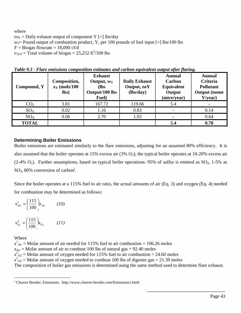
Page 43
where eoY = Daily exhaust output of component Y [=] lbs/day wY= Pound output of combustion product, Y, per 100 pounds of fuel input [=] lbs/100 lbs F = Biogas flowrate = 18,000 cf/d vTOT = Total volume of biogas = 25,252 ft3/100 lbs Table 9.3 - Flare emissions composition estimates and carbon equivalent output after flaring.
Compound, Y Composition, xY (mols/100
lbs)
Exhaust Output, wY
(lbs Output/100 lbs
Fuel)
Daily Exhaust Output, eoY
(lbs/day)
Annual Carbon
Equivalent Output
(mtce/year)
Annual Criteria
Pollutant Output (tonne
Y/year) CO2 3.81 167.72 119.66 5.4 - SOX 0.02 1.16 0.83 - 0.14 NOX 0.06 2.70 1.93 - 0.64
TOTAL 5.4 0.78 Determining Boiler Emissions Boiler emissions are estimated similarly to the flare emissions, adjusting for an assumed 80% efficiency. It is
also assumed that the boiler operates at 15% excess air (3% O2); the typical boiler operates at 10-20% excess air
(2-4% O2). Further assumptions, based on typical boiler operations: 95% of sulfur is emitted as SO2, 1-5% as
SO3, 80% conversion of carbonj.
Since the boiler operates at a 115% fuel to air ratio, the actual amounts of air (Eq. 3) and oxygen (Eq. 4) needed
for combustion may be determined as follows:
AirAir xx ⎟⎠⎞⎜
⎝⎛=1001151 (10)
22 1001152
OO xx ⎟⎠⎞⎜
⎝⎛= (11)
Where x1
Air = Molar amount of air needed for 115% fuel to air combustion = 106.26 moles xAir = Molar amount of air to combust 100 lbs of natural gas = 92.40 moles x2
O2 = Molar amount of oxygen needed for 115% fuel to air combustion = 24.60 moles x1
O2 = Molar amount of oxygen needed to combust 100 lbs of digester gas = 21.39 moles The composition of boiler gas emissions is determined using the same method used to determine flare exhaust.
j Cleaver Brooks: Emissions. http://www.cleaver-brooks.com/Emissions1.html
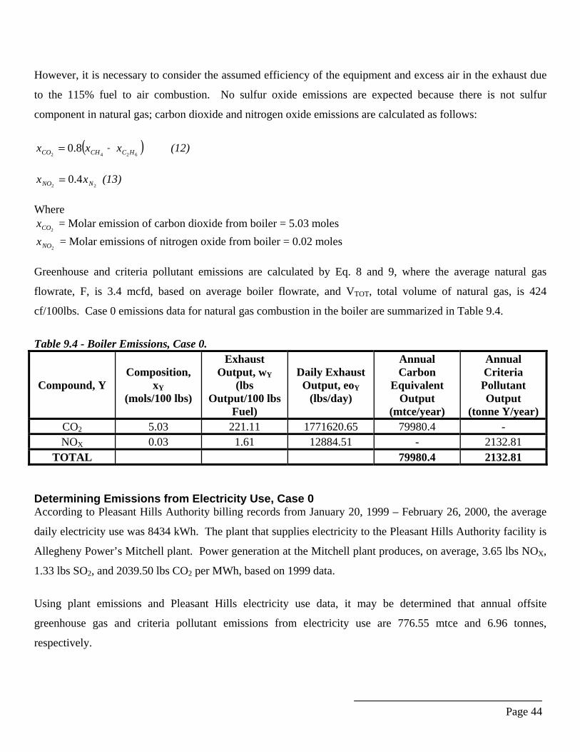
Page 44
However, it is necessary to consider the assumed efficiency of the equipment and excess air in the exhaust due
to the 115% fuel to air combustion. No sulfur oxide emissions are expected because there is not sulfur
component in natural gas; carbon dioxide and nitrogen oxide emissions are calculated as follows:
( )
62428.0 HCCHCO xxx += (12)
22
4.0 NNO xx = (13) Where
2COx = Molar emission of carbon dioxide from boiler = 5.03 moles
2NOx = Molar emissions of nitrogen oxide from boiler = 0.02 moles Greenhouse and criteria pollutant emissions are calculated by Eq. 8 and 9, where the average natural gas
flowrate, F, is 3.4 mcfd, based on average boiler flowrate, and VTOT, total volume of natural gas, is 424
cf/100lbs. Case 0 emissions data for natural gas combustion in the boiler are summarized in Table 9.4.
Table 9.4 - Boiler Emissions, Case 0.
Compound, Y Composition,
xY (mols/100 lbs)
Exhaust Output, wY
(lbs Output/100 lbs
Fuel)
Daily Exhaust Output, eoY
(lbs/day)
Annual Carbon
Equivalent Output
(mtce/year)
Annual Criteria
Pollutant Output
(tonne Y/year) CO2 5.03 221.11 1771620.65 79980.4 - NOX 0.03 1.61 12884.51 - 2132.81
TOTAL 79980.4 2132.81 Determining Emissions from Electricity Use, Case 0 According to Pleasant Hills Authority billing records from January 20, 1999 – February 26, 2000, the average
daily electricity use was 8434 kWh. The plant that supplies electricity to the Pleasant Hills Authority facility is
Allegheny Power’s Mitchell plant. Power generation at the Mitchell plant produces, on average, 3.65 lbs NOX,
1.33 lbs SO2, and 2039.50 lbs CO2 per MWh, based on 1999 data.
Using plant emissions and Pleasant Hills electricity use data, it may be determined that annual offsite
greenhouse gas and criteria pollutant emissions from electricity use are 776.55 mtce and 6.96 tonnes,
respectively.

Page 45
Overall Emissions As may be determined from Tables 9.4, 9.5, and estimated offsite power generation emissions, the Pleasant
Hills Authority facility currently emits 0.39 x 10⁶ mtce and 10.36 x 10³ tonnes of criteria pollutant annually
from flare and boiler operations.
Emissions from Case 1: Hydrogen Sulfide Removal Only In Case 1, the available biogas is stripped of hydrogen sulfide, H2S, and burned in the existing boiler to heat
water. Expected biogas production is 3942 MMBtu/year. It is assumed that the boiler is used for 90% of the
biogas utilization operation, since the boiler may require maintenance. The remaining 10% of the operating
year, the biogas is flared. While some manufacturers and end usersk claim 100% treatment efficiency, a
conservative estimate of 95% treatment efficiency is assumed. The same boiler assumptions are made as for
Case 0.
Analysis of Biogas After Hydrogen Sulfide Removal To determine the change in gas composition, available gas data was normalized for the case that the original
hydrogen sulfide content is reduced by 98%. As may be seen in Table 9.6, hydrogen sulfide content is
negligible after the stripping process. The air and oxygen necessary to combust the treated gas may be
determined using Eq. 3-4.
Table 9.6 - Biogas Composition after Hydrogen Sulfide Stripping
Compound Y
Mole Fraction
MWY (lb/mole)
Weight (lbs)
Mass Fraction
Composition, xy (Mols/100
lbs)
Density-1 (cf/lb)
Volume, vY
(cf/100 lbs)O2 0.97 32 30.93 1.23 0.04 11.82 14.59 N2 2.96 28 82.82 3.31 0.12 7234.07 23921.14
CH4 65.58 16 1049.25 41.89 2.62 23.55 986.61 CO2 30.48 44 1340.95 53.54 1.22 8.55 457.63 H2S 0.02 34 0.77 0.03 0.00 2.26 0.00
TOTAL 100 25380.32
k Reference Library Peroxide Applications: Municipal Wastewater. H2S Control: Scrubbing Hydrogen Sulfide with Hydrogen Peroxide. <http://www.h2o2.com/applications/municipalwastewater/scrubbing.html>
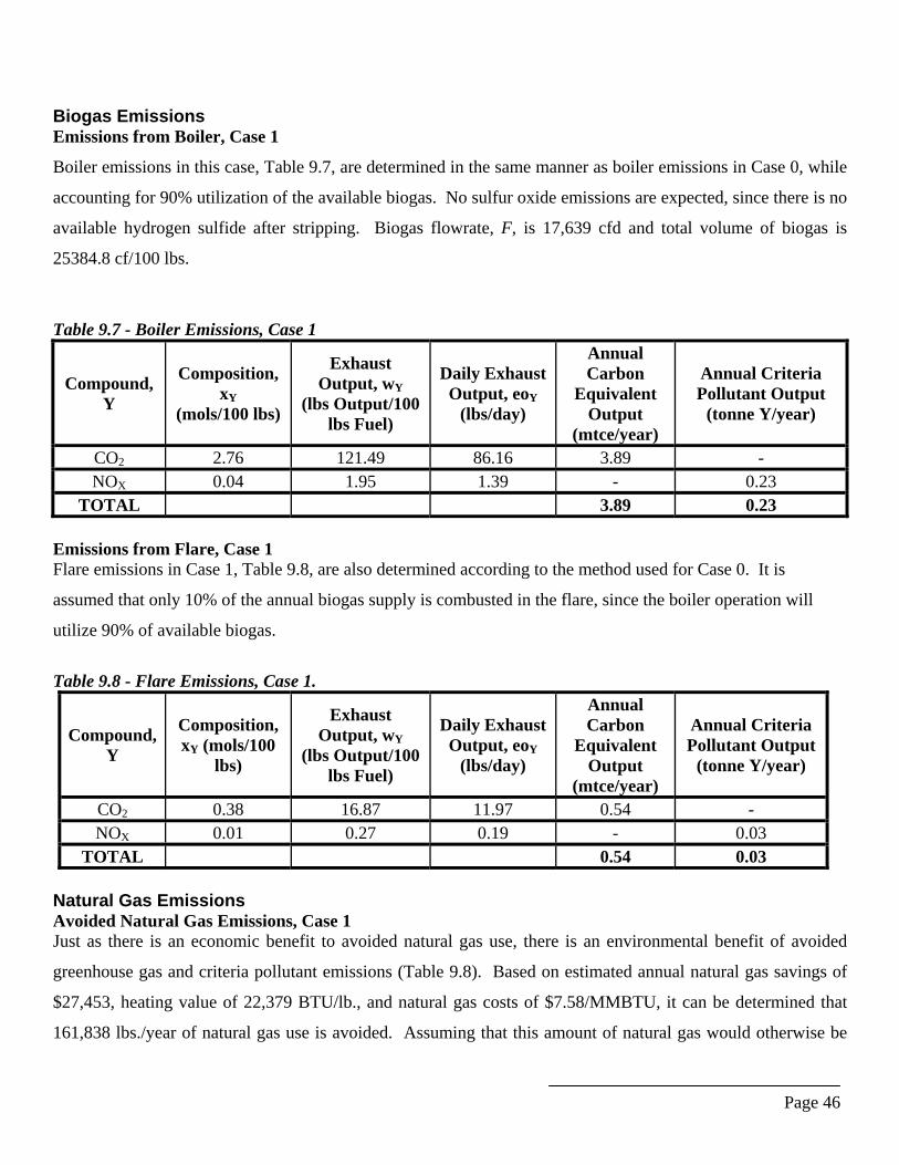
Page 46
Biogas Emissions Emissions from Boiler, Case 1
Boiler emissions in this case, Table 9.7, are determined in the same manner as boiler emissions in Case 0, while
accounting for 90% utilization of the available biogas. No sulfur oxide emissions are expected, since there is no
available hydrogen sulfide after stripping. Biogas flowrate, F, is 17,639 cfd and total volume of biogas is
25384.8 cf/100 lbs.
Table 9.7 - Boiler Emissions, Case 1
Compound, Y
Composition, xY
(mols/100 lbs)
Exhaust Output, wY
(lbs Output/100 lbs Fuel)
Daily Exhaust Output, eoY
(lbs/day)
Annual Carbon
Equivalent Output
(mtce/year)
Annual Criteria Pollutant Output
(tonne Y/year)
CO2 2.76 121.49 86.16 3.89 - NOX 0.04 1.95 1.39 - 0.23
TOTAL 3.89 0.23 Emissions from Flare, Case 1 Flare emissions in Case 1, Table 9.8, are also determined according to the method used for Case 0. It is
assumed that only 10% of the annual biogas supply is combusted in the flare, since the boiler operation will
utilize 90% of available biogas.
Table 9.8 - Flare Emissions, Case 1.
Compound, Y
Composition, xY (mols/100
lbs)
Exhaust Output, wY
(lbs Output/100 lbs Fuel)
Daily Exhaust Output, eoY
(lbs/day)
Annual Carbon
Equivalent Output
(mtce/year)
Annual Criteria Pollutant Output
(tonne Y/year)
CO2 0.38 16.87 11.97 0.54 - NOX 0.01 0.27 0.19 - 0.03
TOTAL 0.54 0.03 Natural Gas Emissions Avoided Natural Gas Emissions, Case 1 Just as there is an economic benefit to avoided natural gas use, there is an environmental benefit of avoided
greenhouse gas and criteria pollutant emissions (Table 9.8). Based on estimated annual natural gas savings of
$27,453, heating value of 22,379 BTU/lb., and natural gas costs of $7.58/MMBTU, it can be determined that
161,838 lbs./year of natural gas use is avoided. Assuming that this amount of natural gas would otherwise be
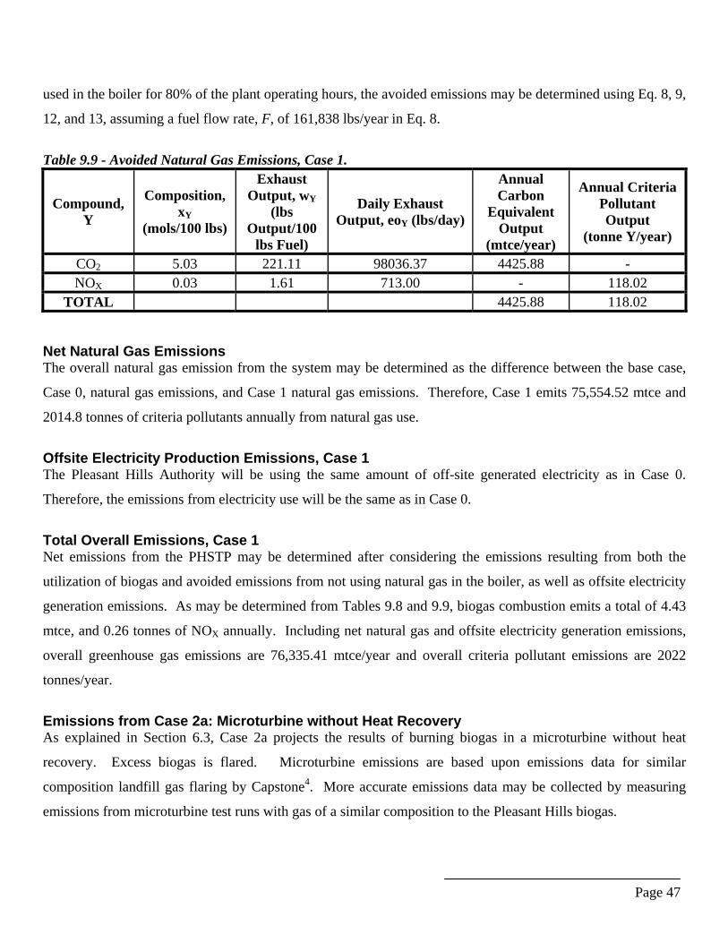
Page 47
used in the boiler for 80% of the plant operating hours, the avoided emissions may be determined using Eq. 8, 9,
12, and 13, assuming a fuel flow rate, F, of 161,838 lbs/year in Eq. 8.
Table 9.9 - Avoided Natural Gas Emissions, Case 1.
Compound, Y
Composition, xY
(mols/100 lbs)
Exhaust Output, wY
(lbs Output/100
lbs Fuel)
Daily Exhaust Output, eoY (lbs/day)
Annual Carbon
Equivalent Output
(mtce/year)
Annual Criteria Pollutant Output
(tonne Y/year)
CO2 5.03 221.11 98036.37 4425.88 - NOX 0.03 1.61 713.00 - 118.02
TOTAL 4425.88 118.02 Net Natural Gas Emissions The overall natural gas emission from the system may be determined as the difference between the base case,
Case 0, natural gas emissions, and Case 1 natural gas emissions. Therefore, Case 1 emits 75,554.52 mtce and
2014.8 tonnes of criteria pollutants annually from natural gas use.
Offsite Electricity Production Emissions, Case 1 The Pleasant Hills Authority will be using the same amount of off-site generated electricity as in Case 0.
Therefore, the emissions from electricity use will be the same as in Case 0.
Total Overall Emissions, Case 1 Net emissions from the PHSTP may be determined after considering the emissions resulting from both the
utilization of biogas and avoided emissions from not using natural gas in the boiler, as well as offsite electricity
generation emissions. As may be determined from Tables 9.8 and 9.9, biogas combustion emits a total of 4.43
mtce, and 0.26 tonnes of NOX annually. Including net natural gas and offsite electricity generation emissions,
overall greenhouse gas emissions are 76,335.41 mtce/year and overall criteria pollutant emissions are 2022
tonnes/year.
Emissions from Case 2a: Microturbine without Heat Recovery As explained in Section 6.3, Case 2a projects the results of burning biogas in a microturbine without heat
recovery. Excess biogas is flared. Microturbine emissions are based upon emissions data for similar
composition landfill gas flaring by Capstone4. More accurate emissions data may be collected by measuring
emissions from microturbine test runs with gas of a similar composition to the Pleasant Hills biogas.
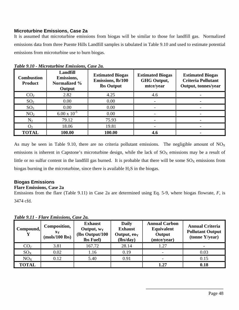
Page 48
Microturbine Emissions, Case 2a It is assumed that microturbine emissions from biogas will be similar to those for landfill gas. Normalized
emissions data from three Puente Hills Landfill samples is tabulated in Table 9.10 and used to estimate potential
emissions from microturbine use to burn biogas.
Table 9.10 - Microturbine Emissions, Case 2a.
Combustion Product
Landfill Emissions,
Normalized % Output
Estimated Biogas Emissions, lb/100
lbs Output
Estimated Biogas GHG Output,
mtce/year
Estimated Biogas Criteria Pollutant
Output, tonnes/year
CO2 2.82 4.25 4.6 - SO2 0.00 0.00 - - SO3 0.00 0.00 - - NO2 6.00 x 10⁻⁵ 0.00 - - N2 79.12 75.93 - - O2 18.06 19.81 - -
TOTAL 100.00 100.00 4.6 - As may be seen in Table 9.10, there are no criteria pollutant emissions. The negligible amount of NOX
emissions is inherent in Capstone’s microturbine design, while the lack of SOX emissions may be a result of
little or no sulfur content in the landfill gas burned. It is probable that there will be some SOX emissions from
biogas burning in the microturbine, since there is available H2S in the biogas.
Biogas Emissions Flare Emissions, Case 2a Emissions from the flare (Table 9.11) in Case 2a are determined using Eq. 5-9, where biogas flowrate, F, is
3474 cfd.
Table 9.11 - Flare Emissions, Case 2a.
Compound, Y
Composition, xY
(mols/100 lbs)
Exhaust Output, wY
(lbs Output/100 lbs Fuel)
Daily Exhaust
Output, eoY (lbs/day)
Annual Carbon Equivalent
Output (mtce/year)
Annual Criteria Pollutant Output
(tonne Y/year)
CO2 3.81 167.72 28.14 1.27 - SOX 0.02 1.16 0.19 - 0.03 NOX 0.12 5.40 0.91 - 0.15
TOTAL 1.27 0.18
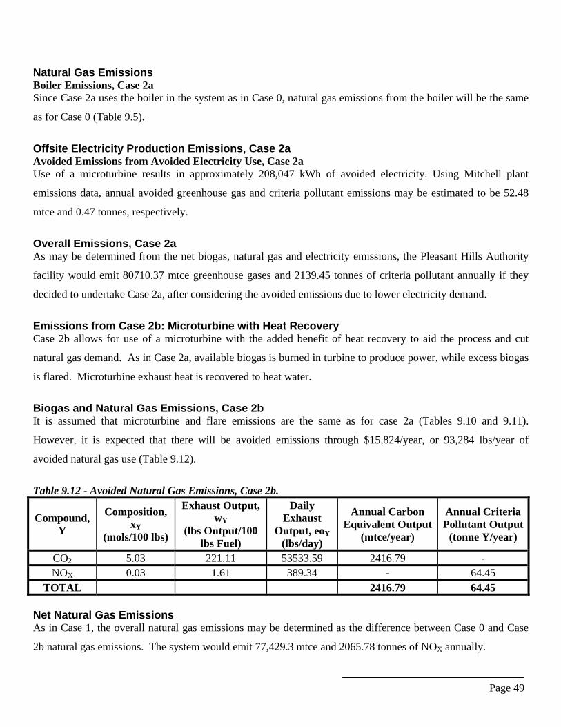
Page 49
Natural Gas Emissions Boiler Emissions, Case 2a Since Case 2a uses the boiler in the system as in Case 0, natural gas emissions from the boiler will be the same
as for Case 0 (Table 9.5).
Offsite Electricity Production Emissions, Case 2a Avoided Emissions from Avoided Electricity Use, Case 2a Use of a microturbine results in approximately 208,047 kWh of avoided electricity. Using Mitchell plant
emissions data, annual avoided greenhouse gas and criteria pollutant emissions may be estimated to be 52.48
mtce and 0.47 tonnes, respectively.
Overall Emissions, Case 2a As may be determined from the net biogas, natural gas and electricity emissions, the Pleasant Hills Authority
facility would emit 80710.37 mtce greenhouse gases and 2139.45 tonnes of criteria pollutant annually if they
decided to undertake Case 2a, after considering the avoided emissions due to lower electricity demand.
Emissions from Case 2b: Microturbine with Heat Recovery Case 2b allows for use of a microturbine with the added benefit of heat recovery to aid the process and cut
natural gas demand. As in Case 2a, available biogas is burned in turbine to produce power, while excess biogas
is flared. Microturbine exhaust heat is recovered to heat water.
Biogas and Natural Gas Emissions, Case 2b It is assumed that microturbine and flare emissions are the same as for case 2a (Tables 9.10 and 9.11).
However, it is expected that there will be avoided emissions through $15,824/year, or 93,284 lbs/year of
avoided natural gas use (Table 9.12).
Table 9.12 - Avoided Natural Gas Emissions, Case 2b.
Compound, Y
Composition, xY
(mols/100 lbs)
Exhaust Output, wY
(lbs Output/100 lbs Fuel)
Daily Exhaust
Output, eoY (lbs/day)
Annual Carbon Equivalent Output
(mtce/year)
Annual Criteria Pollutant Output
(tonne Y/year)
CO2 5.03 221.11 53533.59 2416.79 - NOX 0.03 1.61 389.34 - 64.45
TOTAL 2416.79 64.45 Net Natural Gas Emissions As in Case 1, the overall natural gas emissions may be determined as the difference between Case 0 and Case
2b natural gas emissions. The system would emit 77,429.3 mtce and 2065.78 tonnes of NOX annually.

Page 50
Offsite Electricity Production Emissions, Case 2b Since Case 2b engages the microturbine in the same manner as in Case 2a, the estimated emissions from offsite
electricity generation in Case 2b may be expected to be the same as in Case 2a.
Overall Emissions, Case 2b As may be determined from the summarized net biogas, natural gas and electricity generation emissions,
estimated net emissions from Case 2b are 78,159.27 mtce greenhouse gases and 2071.42 tonnes of criteria
pollutant annually.
Emissions from Case 3: Use of Microturbine, Heat Recovery and Hydrogen Sulfide Removal As explained in Section 6, Case 3 projects the outcome the combined use of a microturbine, heat recovery and
hydrogen sulfide removal. This section summarizes estimates of potential greenhouse gas and criteria pollutant
emissions from Case 3.
Biogas Emissions Microturbine Emissions, Case 3 It is assumed that the microturbine will use treated biogas of the composition tabulated in Table 9.13. However,
for simplicity, the Puente Landfill data is used since there are no SOX emissions from the sample burn data,
which is consistent with expected emissions from Case 3 because hydrogen sulfide is stripped from biogas in
Case 3. More accurate emissions data from the microturbine may be obtained from microturbine and biogas
test burns.
Table 9.13 - Potential Emissions from Microturbine, Case 3.
Combustion Product
Landfill Emissions,
Normalized % Output
Estimated Biogas Emissions, lb/100
lbs Output
Estimated Biogas GHG Output,
mtce/year
Estimated Biogas Criteria Pollutant
Output, tonnes/year
CO2 2.82 4.25 4.6 - SO2 0.00 0.00 - - SO3 0.00 0.00 - - NO2 6.00 x 10⁻⁵ 0.00 - - N2 79.12 75.93 - - O2 18.06 19.81 - -
TOTAL 100.00 100.00 4.6 -
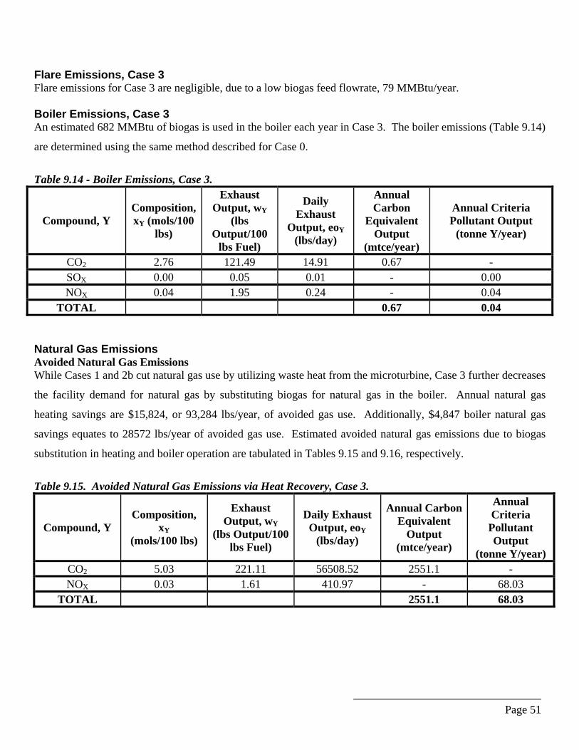
Page 51
Flare Emissions, Case 3 Flare emissions for Case 3 are negligible, due to a low biogas feed flowrate, 79 MMBtu/year. Boiler Emissions, Case 3 An estimated 682 MMBtu of biogas is used in the boiler each year in Case 3. The boiler emissions (Table 9.14)
are determined using the same method described for Case 0.
Table 9.14 - Boiler Emissions, Case 3.
Compound, Y Composition, xY (mols/100
lbs)
Exhaust Output, wY
(lbs Output/100
lbs Fuel)
Daily Exhaust
Output, eoY (lbs/day)
Annual Carbon
Equivalent Output
(mtce/year)
Annual Criteria Pollutant Output
(tonne Y/year)
CO2 2.76 121.49 14.91 0.67 - SOX 0.00 0.05 0.01 - 0.00 NOX 0.04 1.95 0.24 - 0.04
TOTAL 0.67 0.04 Natural Gas Emissions Avoided Natural Gas Emissions While Cases 1 and 2b cut natural gas use by utilizing waste heat from the microturbine, Case 3 further decreases
the facility demand for natural gas by substituting biogas for natural gas in the boiler. Annual natural gas
heating savings are $15,824, or 93,284 lbs/year, of avoided gas use. Additionally, $4,847 boiler natural gas
savings equates to 28572 lbs/year of avoided gas use. Estimated avoided natural gas emissions due to biogas
substitution in heating and boiler operation are tabulated in Tables 9.15 and 9.16, respectively.
Table 9.15. Avoided Natural Gas Emissions via Heat Recovery, Case 3.
Compound, Y Composition,
xY (mols/100 lbs)
Exhaust Output, wY
(lbs Output/100 lbs Fuel)
Daily Exhaust Output, eoY
(lbs/day)
Annual Carbon Equivalent
Output (mtce/year)
Annual Criteria
Pollutant Output
(tonne Y/year) CO2 5.03 221.11 56508.52 2551.1 - NOX 0.03 1.61 410.97 - 68.03
TOTAL 2551.1 68.03
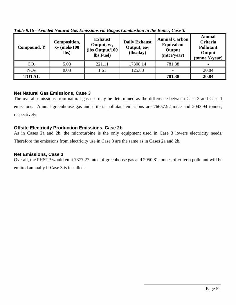
Page 52
Table 9.16 - Avoided Natural Gas Emissions via Biogas Combustion in the Boiler, Case 3.
Compound, Y Composition, xY (mols/100
lbs)
Exhaust Output, wY
(lbs Output/100 lbs Fuel)
Daily Exhaust Output, eoY
(lbs/day)
Annual Carbon Equivalent
Output (mtce/year)
Annual Criteria
Pollutant Output
(tonne Y/year) CO2 5.03 221.11 17308.14 781.38 - NOX 0.03 1.61 125.88 - 20.84
TOTAL 781.38 20.84 Net Natural Gas Emissions, Case 3 The overall emissions from natural gas use may be determined as the difference between Case 3 and Case 1
emissions. Annual greenhouse gas and criteria pollutant emissions are 76657.92 mtce and 2043.94 tonnes,
respectively.
Offsite Electricity Production Emissions, Case 2b As in Cases 2a and 2b, the microturbine is the only equipment used in Case 3 lowers electricity needs.
Therefore the emissions from electricity use in Case 3 are the same as in Cases 2a and 2b.
Net Emissions, Case 3 Overall, the PHSTP would emit 7377.27 mtce of greenhouse gas and 2050.81 tonnes of criteria pollutant will be
emitted annually if Case 3 is installed.
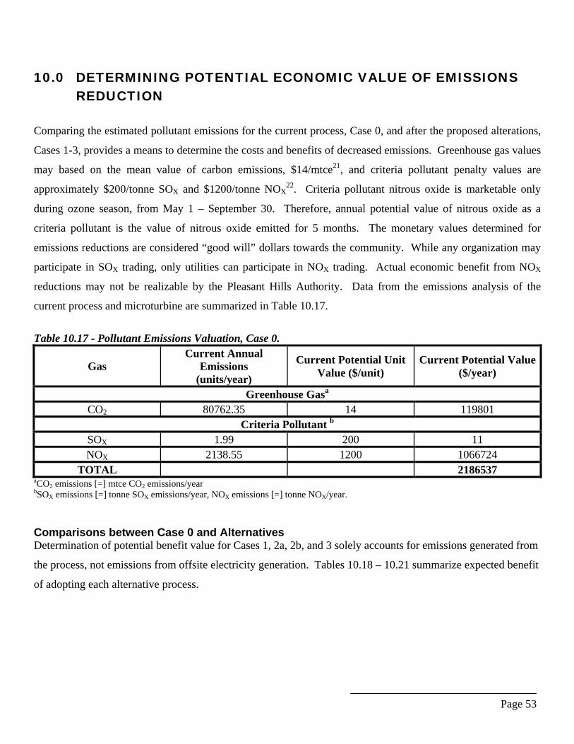
Page 53
10.0 DETERMINING POTENTIAL ECONOMIC VALUE OF EMISSIONS REDUCTION
Comparing the estimated pollutant emissions for the current process, Case 0, and after the proposed alterations,
Cases 1-3, provides a means to determine the costs and benefits of decreased emissions. Greenhouse gas values
may based on the mean value of carbon emissions, $14/mtce21, and criteria pollutant penalty values are
approximately $200/tonne SOX and $1200/tonne NOX22. Criteria pollutant nitrous oxide is marketable only
during ozone season, from May 1 – September 30. Therefore, annual potential value of nitrous oxide as a
criteria pollutant is the value of nitrous oxide emitted for 5 months. The monetary values determined for
emissions reductions are considered “good will” dollars towards the community. While any organization may
participate in SOX trading, only utilities can participate in NOX trading. Actual economic benefit from NOX
reductions may not be realizable by the Pleasant Hills Authority. Data from the emissions analysis of the
current process and microturbine are summarized in Table 10.17.
Table 10.17 - Pollutant Emissions Valuation, Case 0.
Gas Current Annual
Emissions (units/year)
Current Potential Unit Value ($/unit)
Current Potential Value ($/year)
Greenhouse Gasa CO2 80762.35 14 119801
Criteria Pollutant b SOX 1.99 200 11 NOX 2138.55 1200 1066724
TOTAL 2186537 aCO2 emissions [=] mtce CO2 emissions/year bSOX emissions [=] tonne SOX emissions/year, NOX emissions [=] tonne NOX/year. Comparisons between Case 0 and Alternatives Determination of potential benefit value for Cases 1, 2a, 2b, and 3 solely accounts for emissions generated from
the process, not emissions from offsite electricity generation. Tables 10.18 – 10.21 summarize expected benefit
of adopting each alternative process.
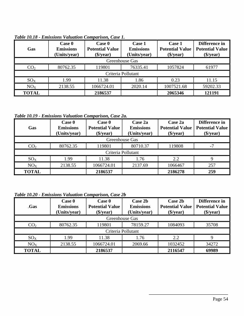
Page 54
Table 10.18 - Emissions Valuation Comparison, Case 1.
Gas Case 0
Emissions (Units/year)
Case 0 Potential Value
($/year)
Case 1 Emissions
(Units/year)
Case 1 Potential Value
($/year)
Difference in Potential Value
($/year) Greenhouse Gas
CO2 80762.35 119801 76335.41 1057824 61977 Criteria Pollutant
SOX 1.99 11.38 1.86 0.23 11.15 NOX 2138.55 1066724.01 2020.14 1007521.68 59202.33
TOTAL 2186537 2065346 121191 Table 10.19 - Emissions Valuation Comparison, Case 2a.
Gas Case 0
Emissions (Units/year)
Case 0 Potential Value
($/year)
Case 2a Emissions
(Units/year)
Case 2a Potential Value
($/year)
Difference in Potential Value
($/year) Greenhouse Gas
CO2 80762.35 119801 80710.37 119808 -7 Criteria Pollutant
SOX 1.99 11.38 1.76 2.2 9 NOX 2138.55 1066724.01 2137.69 1066467 257
TOTAL 2186537 2186278 259 Table 10.20 - Emissions Valuation Comparison, Case 2b
.Gas Case 0
Emissions (Units/year)
Case 0 Potential Value
($/year)
Case 2b Emissions
(Units/year)
Case 2b Potential Value
($/year)
Difference in Potential Value
($/year) Greenhouse Gas
CO2 80762.35 119801 78159.27 1084093 35708 Criteria Pollutant
SOX 1.99 11.38 1.76 2.2 9 NOX 2138.55 1066724.01 2069.66 1032452 34272
TOTAL 2186537 2116547 69989
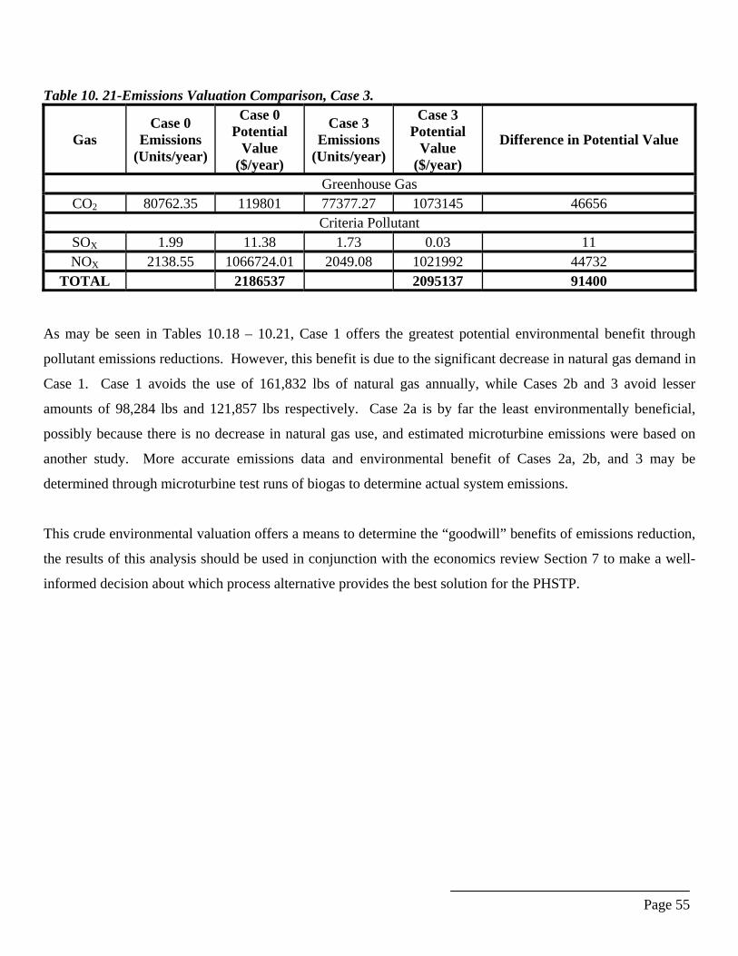
Page 55
Table 10. 21-Emissions Valuation Comparison, Case 3.
Gas Case 0
Emissions (Units/year)
Case 0 Potential
Value ($/year)
Case 3 Emissions
(Units/year)
Case 3 Potential
Value ($/year)
Difference in Potential Value
Greenhouse Gas CO2 80762.35 119801 77377.27 1073145 46656
Criteria Pollutant SOX 1.99 11.38 1.73 0.03 11 NOX 2138.55 1066724.01 2049.08 1021992 44732
TOTAL 2186537 2095137 91400 As may be seen in Tables 10.18 – 10.21, Case 1 offers the greatest potential environmental benefit through
pollutant emissions reductions. However, this benefit is due to the significant decrease in natural gas demand in
Case 1. Case 1 avoids the use of 161,832 lbs of natural gas annually, while Cases 2b and 3 avoid lesser
amounts of 98,284 lbs and 121,857 lbs respectively. Case 2a is by far the least environmentally beneficial,
possibly because there is no decrease in natural gas use, and estimated microturbine emissions were based on
another study. More accurate emissions data and environmental benefit of Cases 2a, 2b, and 3 may be
determined through microturbine test runs of biogas to determine actual system emissions.
This crude environmental valuation offers a means to determine the “goodwill” benefits of emissions reduction,
the results of this analysis should be used in conjunction with the economics review Section 7 to make a well-
informed decision about which process alternative provides the best solution for the PHSTP.
Page 56
11.0 Conclusions and Recommendations
11.1 Conclusions The main objective of this endeavor was to develop a project that could yield economic and environmental benefits for the region with the potential for nationwide replication. In the process, the partnerships developed could lead to problem solutions from which all the project participants could benefit. The problem identified for this project was that a local sewage treatment plant (PHSTP) was flaring the biogas produced in their anaerobic digester. In addition to causing a malodorous problem for the neighbors, the gases released through the flare included CH4 and CO2 which are associated with undesirable global climate change. The flaring of this potential fuel was also a waste of an energy resource. The assembled task group completed a detailed study that determined the technical and economic feasibility of several biogas project options at PHSTP. The overall result of the study was an economically- and technically- viable and environmentally-sound process to capture, clean/dry and utilize all the available biogas. The PHA accepted and embraced the findings from the study and has authorized the project to continue into Phase II, which involves the installation of a turbine/generator/heat recovery assembly at the plant site. The plant will now have the capability to generate some of its own power and co-produce thermal energy to aid in the digester operation. The operating plant and the community of those living and working around the facility will be able experience the most benefits from this effort. The odors emanating from the plant will be reduced significantly. The community will notice some savings in the operating costs of the facility over the next several years and most importantly it will be seen as a community that takes its role as an environmental steward, seriously. The stakeholders who participated on the project team as partners all experienced some level of benefit related to their specific needs and reasons for joining in this effort. The timing of this report comes as parts of the western United States are facing energy-related problems. The information and data gathered from this project may well be used by energy developers as well as policy makers and planners to develop alternate energy source stragegies. Capturing and using this type of energy resource from a waste could be added to the energy mix required in today’s climate of higher energy demands. The development of this energy at the source can relieve some of the pressures on the electric supply grid. This redirecting of energy supplies to other end users can benefit the entire power generation and transmission network. The economic and environmental benefits from this approach are obvious, based on the findings in this report. It is hoped that this report will find its way to help other small communities with similar-sized sewage treatment facilities that could benefit from reduced operating costs. Larger facilities could also benefit as the information presented shows improvements with scale increases due to improved economics. In most cases there will be an environmental benefit that comes with the reduction of the greenhouse gases and criteria pollutants.
11.2 Recommendations This project has shown that public and private partnering can be successful in solving problems and help create opportunities for business growth. NETL plans to continue its efforts in regional development by looking for areas where this type of approach can be utilized. Energy and environmental issues will continue to drive this outreach program.

Page 57
This project will include continued research into evaluating the progress of the implemented options at the facility as a way of verifying the projections stated in this report. It is also recommended that sometime in the near term, negotiations be started to incorporate additional technologies at the facility. Of notable priority would be gas-cleaning and gas-quality upgrading technologies to remove CO2 and other impurities from the digester biogas. CO2 sequestration and reuse options should also be evaluated. This can be approached with a partnering of representatives from local and national interest groups, industry and utilities. 12.0 Bibliography
Page 58
1. Babcock and Wilcox Company. Steam, its generation and use, 38th Ed. New York: 1972.
2. Biegler, Lorenz T., Ignacio E. Grossman, and Arthur W. Westerberg. Systematic Methods of Chemical Process Design. Prentice Hall PTR, Upper Saddle River: 1997.
3. Boyd, James. “The Pollution Prevention Puzzle: Which Policies Will Unlock the Profits?” Resources for
the Future, Spring 1998.
4. Capstone Turbine Corp. Puente Hills Landfill Capstone Turbine Emission Source Testing March 2000. Prepared for: County Sanitation Districts of Los Angeles County. Project No: 2025.1004, Report No: 2025.1004.rpt4.
5. Burtraw, Dallas, Alan Krupnick, Karen Palmer, Anthony Paul, Michael Toman, and Cary Bloyd.
“Ancillary Benefits of Reduced Air Pollution in the U.S. from Moderate Greenhouse Gas Mitigation Policies in the Electricity Sector”. Discussion Paper 99-51, Resources for the Future. September 1999.
6. Cramton, Peter, and Suzi Kerr. “Tradable Carbon Permit Auctions: How and Why to Auction Not
Grandfather”. Discussion Paper 98-34, Resources for the Future. May 1998.
7. Energy Information Administration. “Emissions of Greenhouse Gases in the United States” http://www.eia.doe.gov/oiaf/1605/1605a.html
8. Energy Information Administration. “Emissions of Greenhouse Gases in the United States 1998-
Appendix D: Emissions Sources Excluded” http://www.eia.doe.gov/oiaf/1605/ggrpt/appendixd.html 9. EIA. “Voluntary Reporting of Greenhouse Gases 1998”
http://www.eia.doe.gov/oiaf/1605/vrrpt/index.html 10. EIA. “Voluntary Reporting of Greenhouse Gases 1998- Table 13. Number of Projects and Emission
Reductions” http://www.eia.doe.gov/oiaf/1605/vrrpt/table_13.html 11. EPA Environmental Policy Alert. “EPA Makes Hydrogen Sulfide Effort Model for Future HAP
Listings”. March 8, 2000. 12. EPA. “State-Authored GHG Inventories”
http://yosemite.epa.gov/globalwarming/ghg.nsf/emissions/StateAuthoredInventories?Open 13. EPA. “Pennsylvania Greenhouse Gas Emissions and Sinks Inventory: Summary”
http://yosemite.epa.gov/globalwarming/ghg.nsf/resources/PDFs/$file/PASummary.PDF
14. EPA. “U.S. Methane Emissions 1990-2020: Inventories, Projections, and Opportunities for Reductions” Office of Air and Radiation. EPA 430-R-99-O13, September 1999. http://www.epa.gov/globalwarming/publications/emissions/methane_emissions.pdf
15. Fristrom, R.M. Flame Structure and Processes, Oxford University Press, New York: 1995.

Page 59
16. Grubb, Michael. “Technologies, energy systems and the timing of CO2 emissions abatement” Energy Policy, Vol. 25, No. 2, pp. 159-172, 1997.
17. ICF Consulting. “Methods for Estimating Greenhouse Gas Emissions from Municipal Wastewater”
Emissions Inventory Improvement Program Volume VIII: Chapter 12. October 1999. 18. Kandlikar, Milind. “Greenhouse Gas Indices” Degrees of Change: A Newsletter from the Global
Change Integrated Assessment Program. Department of Engineering & Public Policy, Carnegie Mellon. Vol. 1(4), May 1996.
19. Klein, Daniel. Suitability of Methane Sources for Emissions Trading. Twenty-First Strategies, LLC,
Prepared for the Center for Clean Air Policy’s Greenhouse Gas Emissions Trading Brain trust. Draft, 2/9/00.
20. Koe, Lawrence C.C. “Sewage Odors Quantification” Encyclopedia of Environmental Control
Technology, Vol. 3: Wastewater Treatment Technology. Chapter 15, pp. 423-446. Gulf Publishing Company, Houston: 1989.
21. Matthews, H. Scott. “The External Costs of air Pollution and the environmental Impact of the Consumer
in the U.S. Economy” Dissertation. Graduate School of Industrial Administration, Carnegie Mellon University, March 1999.
22. McGraw-Hill Companies’ Utility Environment Report. The McGraw-Hill Companies, Inc. September
10, 1999.
23. National Resources Defense Council. “Getting the Dirt on Your Electric Company: Allegheny Power” http://www.nrdc.org/air/energy/utilprof/al.asp.
24. North American Mfg. Co. North American Combustion Handbook: A Basic Reference on the Art and
Science of Industrial Heating with Gaseous and Liquid Fuels, Volume I: Combustion, Fuels, Stoichiometry, Heat Transfer, Fluid Flow. Third edition, p. 212.
25. Reference Library Peroxide Applications: Municipal Wastewater. “H2S Control: Scrubbing Hydrogen
Sulfide with Hydrogen Peroxide”. http://www.h2o2.com/applications/municipalwastewater/scrubbing.html
26. Stevens, William K. “Agreement is Reached in Kyoto on Greenhouse Gases” New York Times,
December 11, 1997.
27. U.S. Senate Committee on Environment and Public Works. Hearing on Voluntary Activities to Reduce the Emission of Greenhouse Gases. March 24, 1999.

Page 60
13.0 Nomenclature Btu British thermal unit CF cubic foot DOE Department of Energy H2S hydrogen sulfide IRR internal rate of return kW kilowatt kWh kilowatt-hour LCC life cycle cost LHV lower heating value MCF thousand cubic feet MMBtu million British thermal units NETL National Energy Technology Laboratory NPV net present value PHA Pleasant Hills Authority psig pounds per square inch, gauge
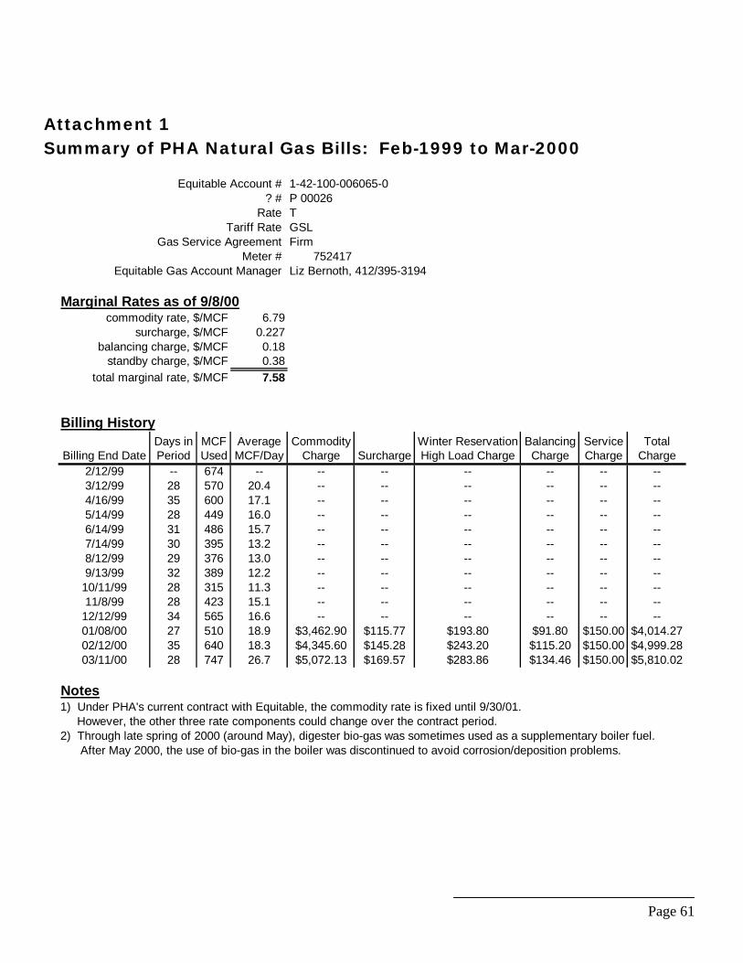
Page 61
Attachment 1 Summary of PHA Natural Gas Bills: Feb-1999 to Mar-2000
Equitable Account # 1-42-100-006065-0 ? # P 00026
Rate TTariff Rate GSL
Gas Service Agreement FirmMeter # 752417
Equitable Gas Account Manager Liz Bernoth, 412/395-3194
Marginal Rates as of 9/8/00commodity rate, $/MCF 6.79
surcharge, $/MCF 0.227balancing charge, $/MCF 0.18
standby charge, $/MCF 0.38total marginal rate, $/MCF 7.58
Billing HistoryDays in MCF Average Commodity Winter Reservation Balancing Service Total
Billing End Date Period Used MCF/Day Charge Surcharge High Load Charge Charge Charge Charge2/12/99 -- 674 -- -- -- -- -- -- --3/12/99 28 570 20.4 -- -- -- -- -- --4/16/99 35 600 17.1 -- -- -- -- -- --5/14/99 28 449 16.0 -- -- -- -- -- --6/14/99 31 486 15.7 -- -- -- -- -- --7/14/99 30 395 13.2 -- -- -- -- -- --8/12/99 29 376 13.0 -- -- -- -- -- --9/13/99 32 389 12.2 -- -- -- -- -- --
10/11/99 28 315 11.3 -- -- -- -- -- --11/8/99 28 423 15.1 -- -- -- -- -- --
12/12/99 34 565 16.6 -- -- -- -- -- --01/08/00 27 510 18.9 $3,462.90 $115.77 $193.80 $91.80 $150.00 $4,014.2702/12/00 35 640 18.3 $4,345.60 $145.28 $243.20 $115.20 $150.00 $4,999.2803/11/00 28 747 26.7 $5,072.13 $169.57 $283.86 $134.46 $150.00 $5,810.02
Notes1) Under PHA's current contract with Equitable, the commodity rate is fixed until 9/30/01. However, the other three rate components could change over the contract period.2) Through late spring of 2000 (around May), digester bio-gas was sometimes used as a supplementary boiler fuel. After May 2000, the use of bio-gas in the boiler was discontinued to avoid corrosion/deposition problems.
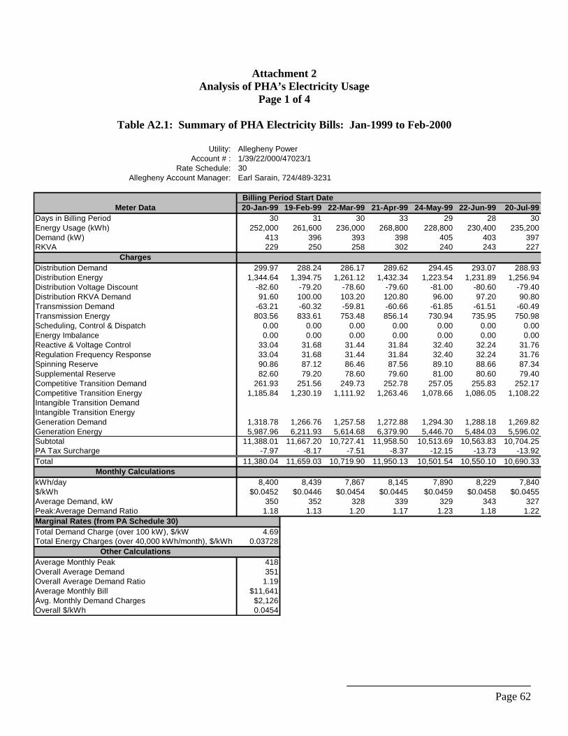
Page 62
Attachment 2 Analysis of PHA’s Electricity Usage
Page 1 of 4
Table A2.1: Summary of PHA Electricity Bills: Jan-1999 to Feb-2000
Utility: Allegheny PowerAccount # : 1/39/22/000/47023/1
Rate Schedule: 30Allegheny Account Manager: Earl Sarain, 724/489-3231
Billing Period Start DateMeter Data 20-Jan-99 19-Feb-99 22-Mar-99 21-Apr-99 24-May-99 22-Jun-99 20-Jul-99
Days in Billing Period 30 31 30 33 29 28 30Energy Usage (kWh) 252,000 261,600 236,000 268,800 228,800 230,400 235,200Demand (kW) 413 396 393 398 405 403 397RKVA 229 250 258 302 240 243 227
ChargesDistribution Demand 299.97 288.24 286.17 289.62 294.45 293.07 288.93Distribution Energy 1,344.64 1,394.75 1,261.12 1,432.34 1,223.54 1,231.89 1,256.94Distribution Voltage Discount -82.60 -79.20 -78.60 -79.60 -81.00 -80.60 -79.40Distribution RKVA Demand 91.60 100.00 103.20 120.80 96.00 97.20 90.80Transmission Demand -63.21 -60.32 -59.81 -60.66 -61.85 -61.51 -60.49Transmission Energy 803.56 833.61 753.48 856.14 730.94 735.95 750.98Scheduling, Control & Dispatch 0.00 0.00 0.00 0.00 0.00 0.00 0.00Energy Imbalance 0.00 0.00 0.00 0.00 0.00 0.00 0.00Reactive & Voltage Control 33.04 31.68 31.44 31.84 32.40 32.24 31.76Regulation Frequency Response 33.04 31.68 31.44 31.84 32.40 32.24 31.76Spinning Reserve 90.86 87.12 86.46 87.56 89.10 88.66 87.34Supplemental Reserve 82.60 79.20 78.60 79.60 81.00 80.60 79.40Competitive Transition Demand 261.93 251.56 249.73 252.78 257.05 255.83 252.17Competitive Transition Energy 1,185.84 1,230.19 1,111.92 1,263.46 1,078.66 1,086.05 1,108.22Intangible Transition DemandIntangible Transition EnergyGeneration Demand 1,318.78 1,266.76 1,257.58 1,272.88 1,294.30 1,288.18 1,269.82Generation Energy 5,987.96 6,211.93 5,614.68 6,379.90 5,446.70 5,484.03 5,596.02Subtotal 11,388.01 11,667.20 10,727.41 11,958.50 10,513.69 10,563.83 10,704.25PA Tax Surcharge -7.97 -8.17 -7.51 -8.37 -12.15 -13.73 -13.92Total 11,380.04 11,659.03 10,719.90 11,950.13 10,501.54 10,550.10 10,690.33
Monthly CalculationskWh/day 8,400 8,439 7,867 8,145 7,890 8,229 7,840$/kWh $0.0452 $0.0446 $0.0454 $0.0445 $0.0459 $0.0458 $0.0455Average Demand, kW 350 352 328 339 329 343 327Peak:Average Demand Ratio 1.18 1.13 1.20 1.17 1.23 1.18 1.22Marginal Rates (from PA Schedule 30)Total Demand Charge (over 100 kW), $/kW 4.69Total Energy Charges (over 40,000 kWh/month), $/kWh 0.03728
Other CalculationsAverage Monthly Peak 418Overall Average Demand 351Overall Average Demand Ratio 1.19Average Monthly Bill $11,641Avg. Monthly Demand Charges $2,126Overall $/kWh 0.0454

Page 63
Attachment 2: Page 2 of 4
Table A2.1 (continued): Summary of PHA Electricity Bills: Jan-1999 to Feb-2000
Billing Period Start Date
Meter Data 19-Aug-99 22-Sep-99 20-Oct-99 19-Nov-99 22-Dec-99 21-Jan-00 22-Feb-00Days in Billing Period 34 28 30 33 30 32 28Energy Usage (kWh) 280,000 238,400 256,000 292,800 281,600 305,600 225,600Demand (kW) 418 431 441 456 436 459 408RKVA 263 253 272 277 249 253 244
ChargesDistribution Demand 303.42 312.39 319.29 329.64 352.46 386.79 345.48Distribution Energy 1,490.80 1,273.65 1,365.52 1,557.62 1,692.33 1,923.92 1,427.92Distribution Voltage Discount -83.60 -86.20 -88.20 -91.20 -87.20 -91.80 -81.60Distribution RKVA Demand 105.20 101.20 108.80 110.80 99.60 101.20 97.60Transmission Demand -64.06 -66.27 -67.97 -70.52 -67.12 -71.03 -62.36Transmission Energy 891.20 760.99 816.08 931.26 896.21 971.33 720.93Scheduling, Control & Dispatch 0.00 0.00 0.00 0.00 0.00 0.00 0.00Energy Imbalance 0.00 0.00 0.00 0.00 0.00 0.00 0.00Reactive & Voltage Control 33.44 34.48 35.28 36.48 34.88 36.72 32.64Regulation Frequency Response 33.44 34.48 35.28 36.48 34.88 36.72 32.64Spinning Reserve 91.96 94.82 97.02 100.32 95.92 100.98 89.76Supplemental Reserve 83.60 86.20 88.20 91.20 87.20 91.80 81.60Competitive Transition Demand 264.98 272.91 244.16 18.24 11.34 9.18 8.16Competitive Transition Energy 1,315.20 1,123.01 1,060.16 140.42 105.02 99.79 74.19Intangible Transition Demand 34.85 269.92 258.52 271.63 242.56Intangible Transition Energy 144.16 1,233.92 1,187.44 1,287.04 955.04Generation Demand 1,334.08 1,373.86 1,404.46 1,450.36 1,395.26 1,468.72 1,311.64Generation Energy 6,641.20 5,670.67 6,081.28 6,939.82 6,708.66 7,285.09 5,406.69Subtotal 12,440.86 10,986.19 11,678.37 13,084.76 12,805.40 13,908.08 10,682.89PA Tax Surcharge -16.17 -14.28 -15.18 -17.01 -4.91 0.00 0.00Total 12,424.69 10,971.91 11,663.19 13,067.75 12,800.49 13,908.08 10,682.89
Monthly CalculationskWh/day 8,235 8,514 8,533 8,873 9,387 9,550 8,057$/kWh $0.0444 $0.0460 $0.0456 $0.0446 $0.0455 $0.0455 $0.0474Average Demand, kW 343 355 356 370 391 398 336Peak:Average Demand Ratio 1.22 1.21 1.24 1.23 1.11 1.15 1.22
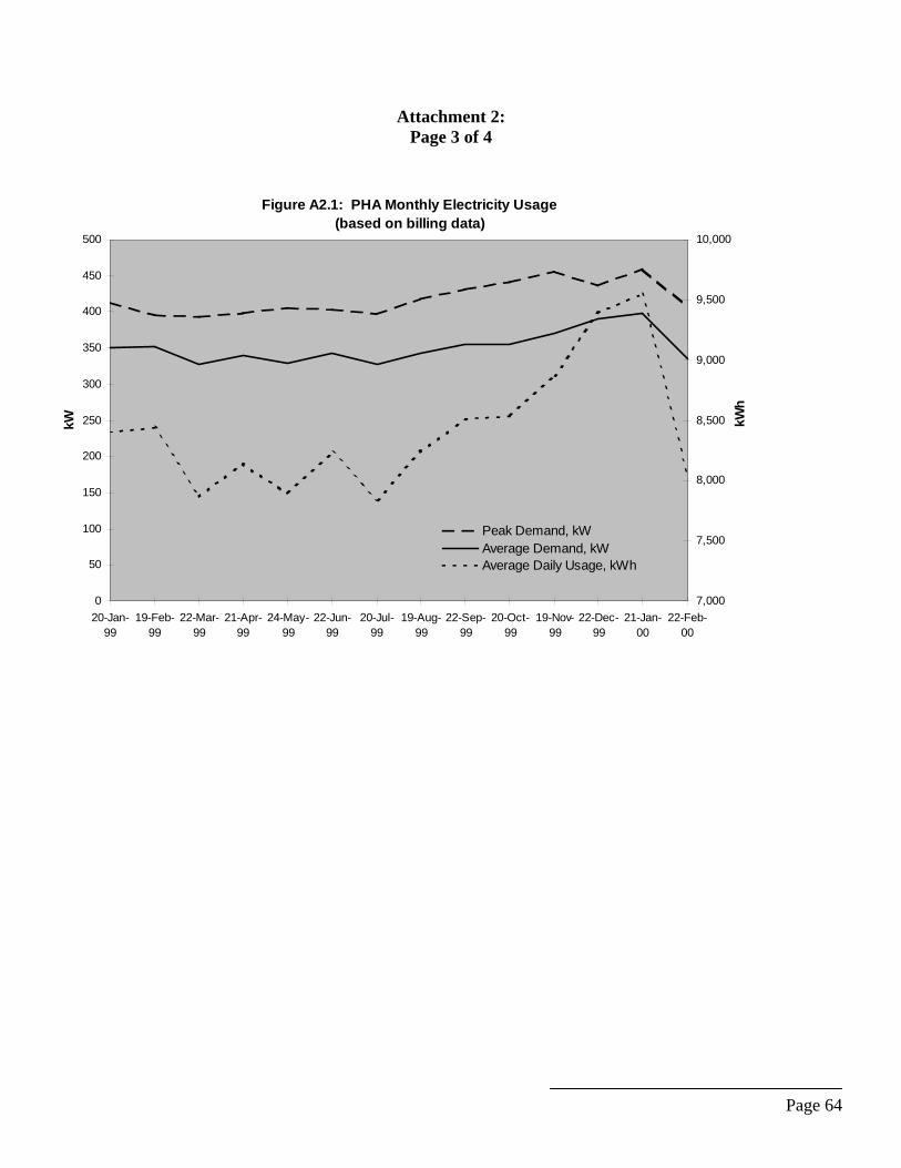
Page 64
Attachment 2: Page 3 of 4
Figure A2.1: PHA Monthly Electricity Usage(based on billing data)
0
50
100
150
200
250
300
350
400
450
500
20-Jan-99
19-Feb-99
22-Mar-99
21-Apr-99
24-May-99
22-Jun-99
20-Jul-99
19-Aug-99
22-Sep-99
20-Oct-99
19-Nov-99
22-Dec-99
21-Jan-00
22-Feb-00
kW
7,000
7,500
8,000
8,500
9,000
9,500
10,000
kWh
Peak Demand, kWAverage Demand, kWAverage Daily Usage, kWh
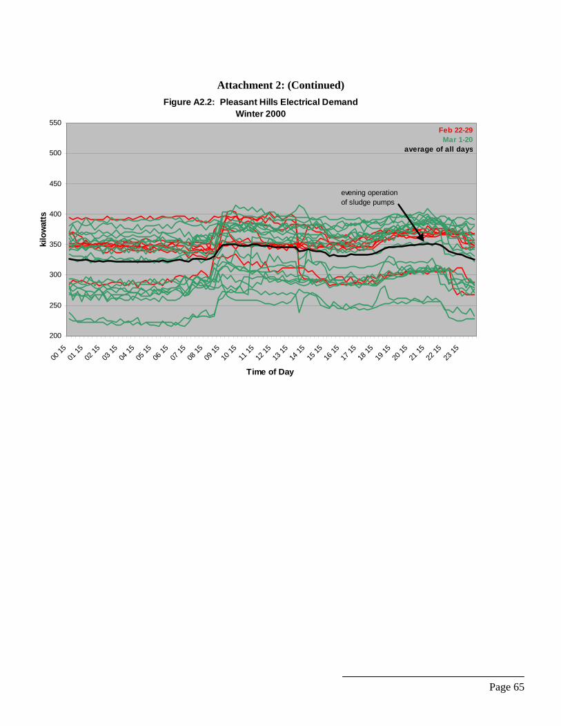
Page 65
Attachment 2: (Continued)
Figure A2.2: Pleasant Hills Electrical DemandWinter 2000
200
250
300
350
400
450
500
550
00 15
01 15
02 15
03 15
04 15
05 15
06 15
07 15
08 15
09 15
10 15
11 15
12 15
13 15
14 15
15 15
16 15
17 15
18 15
19 15
20 15
21 15
22 15
23 15
Time of Day
kilo
wat
ts
Feb 22-29Mar 1-20
average of all days
evening operationof sludge pumps
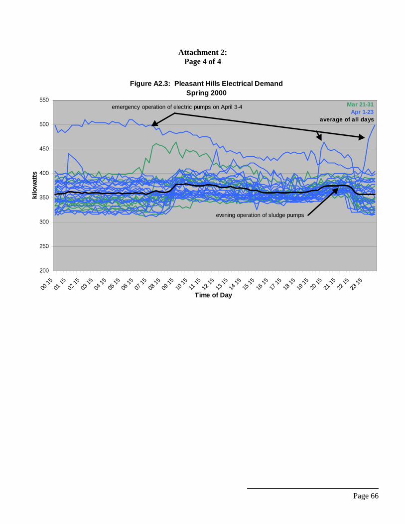
Page 66
Attachment 2: Page 4 of 4
Figure A2.3: Pleasant Hills Electrical Demand
Spring 2000
200
250
300
350
400
450
500
550
00 15
01 15
02 15
03 15
04 15
05 15
06 15
07 15
08 15
09 15
10 15
11 15
12 15
13 15
14 15
15 15
16 15
17 15
18 15
19 15
20 15
21 15
22 15
23 15
Time of Day
kilo
wat
ts
Mar 21-31Apr 1-23
average of all days
evening operation of sludge pumps
emergency operation of electric pumps on April 3-4

Page 67
Attachment 3 Capstone Turbine Corporation Equipment Specification Sheets
(not included electronically; hard copies inserted)