petri nets for modelling and analysing trophic networks · martina bocci,daniele brigolin,...
TRANSCRIPT

Petri nets for modelling and analysing Trophicnetworks
Marta Simeoni
Universita Ca’ Foscari Venezia
L’Aquila, March 9, 2018
Joint work withPaolo Baldan (Universita Padova),
Monika Heiner (Brandenburg University of Technology, Cottbus, Germany)Martina Bocci, Daniele Brigolin, and Nicoletta Cocco (Universita Ca’ Foscari Venezia)

Framework
Ecosystem = community of living organisms + nonlivingcomponents of the environment
A trophic network (or food web) is a representation of the feedinginteractions in an ecosystem (what-eats-what)
Let’s employ Petri nets in this framework!

Framework
Ecosystem = community of living organisms + nonlivingcomponents of the environment
A trophic network (or food web) is a representation of the feedinginteractions in an ecosystem (what-eats-what)
Let’s employ Petri nets in this framework!

Trophic networks
They are represented as directed graphs where:
I each node represents a species or a group of species(compartment) with similar feeding behaviour;
I each arc denotes a flow of biomass or energy from the sourcenode to the target one
They are usually open systems:
I input flows, e.g, primary production, immigration, incoming ofdetrital matter into the system
I output flows, e.g. respiration, emigration, harvesting byhumans, exit of detrital matter from the system
Trophic networks
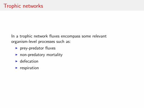
In a trophic network fluxes encompass some relevantorganism-level processes such as:
I prey-predator fluxes
I non-predatory mortality
I defecation
I respiration

A simple planktonic trophic network of the Venice Lagoon
I TAP = R. philippinarum,a clam living on the bottom
I MEZ = ”large” zooplankton
I MIZ = small zooplankton
I BPL = bacteria
I PHP = phytoplankton
I DET = detritus(dead organic matter)

Trophic networks: quantitative data
It is possible to add quantitative data:
I Some quantitative information can be derived from theliterature or gained from field or laboratory studies(e.g. diet composition, information on consumption,information on primary production)
However, it is unfeasible to determine the magnitudes of all flowsin the system directly

Trophic networks: estimating quantitative data
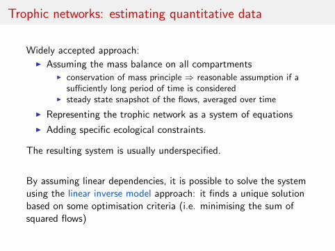
Widely accepted approach:I Assuming the mass balance on all compartments
I conservation of mass principle ⇒ reasonable assumption if asufficiently long period of time is considered
I steady state snapshot of the flows, averaged over time
I Representing the trophic network as a system of equations
I Adding specific ecological constraints.
The resulting system is usually underspecified.
By assuming linear dependencies, it is possible to solve the systemusing the linear inverse model approach: it finds a unique solutionbased on some optimisation criteria (i.e. minimising the sum ofsquared flows)
Trophic networks: estimating quantitative data
Widely accepted approach:I Assuming the mass balance on all compartments
I conservation of mass principle ⇒ reasonable assumption if asufficiently long period of time is considered
I steady state snapshot of the flows, averaged over time
I Representing the trophic network as a system of equations
I Adding specific ecological constraints.
The resulting system is usually underspecified.
By assuming linear dependencies, it is possible to solve the systemusing the linear inverse model approach: it finds a unique solutionbased on some optimisation criteria (i.e. minimising the sum ofsquared flows)
Analysis of trophic networks
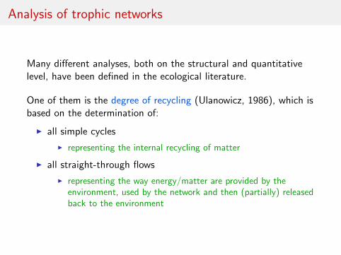
Many different analyses, both on the structural and quantitativelevel, have been defined in the ecological literature.
One of them is the degree of recycling (Ulanowicz, 1986), which isbased on the determination of:
I all simple cycles
I representing the internal recycling of matter
I all straight-through flows
I representing the way energy/matter are provided by theenvironment, used by the network and then (partially) releasedback to the environment

Petri nets (PNs)
I First introduced in 1962 by CarlAdam Petri for describing chemicalprocesses
I A diagrammatic tool to modelconcurrency and synchronisation indistributed systems
I Used as a visual communicationaid to model the system behaviour
I Based on strong mathematicalfoundation
Components of a PN
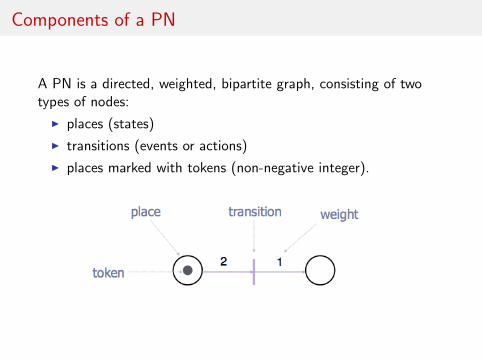
A PN is a directed, weighted, bipartite graph, consisting of twotypes of nodes:
I places (states)
I transitions (events or actions)
I places marked with tokens (non-negative integer).
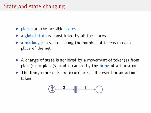
State and state changing
I places are the possible states
I a global state is constituted by all the places
I a marking is a vector listing the number of tokens in eachplace of the net
I A change of state is achieved by a movement of token(s) fromplace(s) to place(s) and is caused by the firing of a transition
I The firing represents an occurrence of the event or an actiontaken

Behaviour
I a transition may fire when it is enabled
I a transition is enabled when each of its input places contain atleast as many tokens as the weight of the corresponding inputarc
I firing depends only on the local state of input places(pre-condition) and it affects the local state of input andoutput places (pos-tcondition)
I firing is atomic, namely it is a non-interruptible step
I firing is immediate in basic Petri nets
I An enabled transition may or may not fire (nondeterminism).

Incidence Matrix
The Incidence Matrix of a PN is a matrix with a row for each placeand a column for each transition. The k-th matrix column is thevector representing the marking change when Tk fires.

Analysis of Petri nets
PNs used for modelling and analysing complex systems
I Analysis allows for model validation and for studyingproperties of the modelled system
I Analysis can be performed at different levelsI structural analysis
structural properties only depend on the net topologyI behavioural analysis
behavioural properties depend on the evolution of the net froman initial state (marking)
I simulationallows for running the network

Structural analysis of PNs: T-invariants
A T-invariant of a Petri net N is an m-dimensional vector in whicheach component represents the number of times that a transitionshould fire to take the net from a state M back to M itself. It canbe obtained as a solution of the following equation:
ANX = 0
where X = (x1, . . . , xm)T and xi natural number for i = 1. . . m
A T-invariant X 6= 0 indicates that the system can cycle on a stateM enabling the cycle.
The presence of a T-invariant in a PN can reveal the presence of asteady state in the involved subnet.

Structural analysis of PNs: T-invariants
I In general a PN admits more than one T- invariant
I A T-invariant is minimum if there does not exist a differentinvariant whose support (non-zero components) is a subset ofthe given T-invariant.
I A linear combination of invariants is still an invariant.
The set of minimal T-invariants of a PN is called Hilbert Basis.
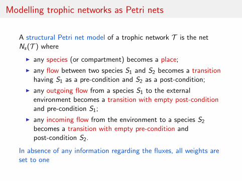
Modelling trophic networks as Petri nets
A structural Petri net model of a trophic network T is the netNs(T ) where
I any species (or compartment) becomes a place;
I any flow between two species S1 and S2 becomes a transitionhaving S1 as a pre-condition and S2 as a post-condition;
I any outgoing flow from a species S1 to the externalenvironment becomes a transition with empty post-conditionand pre-condition S1;
I any incoming flow from the environment to a species S2
becomes a transition with empty pre-condition andpost-condition S2.
In absence of any information regarding the fluxes, all weights areset to one

The Petri net of the Venice Lagoon
Colours legend:Yellow places = CompartmentsRed transitions = Interface flowsLight blue transitions = Respiration flowsBrown transitions = Defecation flowsPurple transitions = Death flowsWhite transitions = Consumption flows

Analysis of trophic networks represented as Petri nets
Given a trophic network T , consider the corresponding Hilbertbasis B(Ns(T )). For any T-invariant of the basis:
I Minimal internal invariants are simple cycles, involving onlyinternal transitions⇒ correspond to Ulanowicz simple cycles
I Minimal I/O invariants are acyclic paths, connecting twointerface transitions⇒ correspond to Ulanowicz straight-through flows
The Petri net model of the Venice Lagoon has 69 minimalT-invariants: nine internal and sixty I/O invariants.

Continuous Petri net model of a trophic network
We refine the structural Petri net model turning it into acontinuous Petri net model
I derived from the network topology by exploiting theminimal T-invariants in a way similar to what is donein (Popova-Zeugmann, Heiner, and Koch, 2005)
The structural Petri net model of a trophic network is covered byT-invariants
I under the assumption that any place has at least oneincoming and one outgoing transition
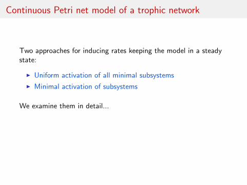
Continuous Petri net model of a trophic network
Two approaches for inducing rates keeping the model in a steadystate:
I Uniform activation of all minimal subsystems
I Minimal activation of subsystems
We examine them in detail...

First Continuous Petri net model of a trophic network
Uniform activation of all minimal subsystems: each subsystemcorresponding to a minimal T-invariant
I is active⇒ reasonable assumption from an ecological viewpoint
I performs all its transitions once per time unit⇒ rather strong and unrealistic assumption

Uniform Continuous Petri net model of a trophic network
The uniform continuous Petri net model Nc(T ) is the continuousPetri net obtained by
I considering the structural model Ns(T ) as underlying Petri net
I associating to each transition t a constant rate given by:
rate(t) = |{Ii |Ii ∈ B(Ns(T )) ∧ t ∈ Ii}|.
Then:
I all the transitions in all the invariants in Nc(T ) are performedonce in one time unit and the system is in a steady state;
I since all transition arcs are 1-weighted, rates and flows pertime unit coincide;
I for each compartment the sum of incoming and outgoingfluxes coincide, i.e. the mass balance assumption is satisfied

Uniform continuous Petri net of the Venice Lagoon
REMARKS:The structure of the trophic network is unique and it is depicted above, but there are 5 different function sets for the transitions rates (i.e. there are actually 5 different models).
−−−−−−−The Prey−Predator activity is modelled with standard arcs by: Prey −−−> || −−2−> Predator <−−1− This modelling technique is needed only for the mass−dependent rates (the mass−action law considers the marking of the pre−places only). It has no influence on the other models.
Petri net model of the Venice lagoon food web, case study of the paper.−−−Yellow places = internal placesRed transition = interface White transition = consumption (prey−predator activity)Blue transition = respirationBrown transition = feacesPurple transition = death−−−
BPL
DET
MEZ
MIZ
PHP
TAP
DET_TAP
11
TAP_CO2
15
TAP_DET
11
MEZ_CO210
MEZ_DET
17
MEZ_MEZ
1
MIZ_TAP
12
MIZ_MEZ
11
MIZ_CO2
5
MIZ_DET
8
MIZ_MIZ
1
BPL_TAP
11
BPL_MIZ
16
BPL_MEZ6
BPL_CO2
7
DET_BPL
41PHP_TAP
7
PHP_MEZ
10
PHP_MIZ
20
PHP_DET
11
CO2_PHP
49
TAP_harvesting15
DET_export
7
input_DET
11
BPL_DET
1
PHP_CO2
1
Colours legend:Yellow places = CompartmentsRed transitions = Interface flowsLight blue transitions = Respiration flowsBrown transitions = Defecation flowsPurple transitions = Death flowsWhite transitions = Consumption flows

Ecological validation of the uniform continuous VeniceLagoon model
For each compartment, we consider some basic ecologicalprocesses:
I throughput: total amount of flux flowing per time unit
I consumption: total amount of ingested food per time unit
I assimilation: total amount of ingested food minus amount offeaces, per time unit
I respiration
We check their plausibility from an ecological point of view
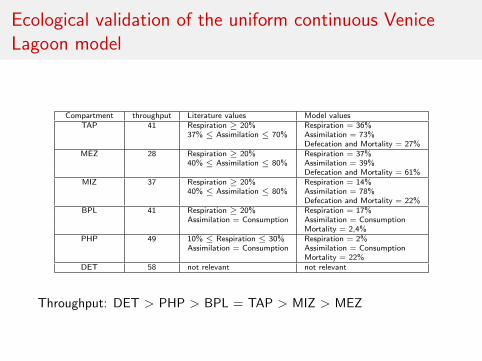
Ecological validation of the uniform continuous VeniceLagoon model
Compartment throughput Literature values Model valuesTAP 41 Respiration ≥ 20% Respiration = 36%
37% ≤ Assimilation ≤ 70% Assimilation = 73%Defecation and Mortality = 27%
MEZ 28 Respiration ≥ 20% Respiration = 37%40% ≤ Assimilation ≤ 80% Assimilation = 39%
Defecation and Mortality = 61%MIZ 37 Respiration ≥ 20% Respiration = 14%
40% ≤ Assimilation ≤ 80% Assimilation = 78%Defecation and Mortality = 22%
BPL 41 Respiration ≥ 20% Respiration = 17%Assimilation = Consumption Assimilation = Consumption
Mortality = 2,4%PHP 49 10% ≤ Respiration ≤ 30% Respiration = 2%
Assimilation = Consumption Assimilation = ConsumptionMortality = 22%
DET 58 not relevant not relevant
Throughput: DET > PHP > BPL = TAP > MIZ > MEZ
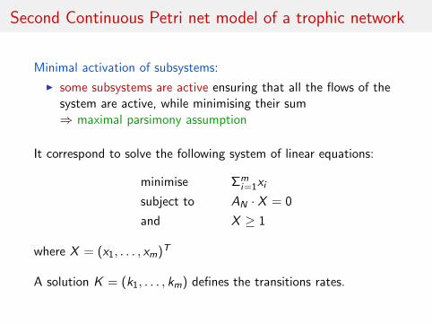
Second Continuous Petri net model of a trophic network
Minimal activation of subsystems:
I some subsystems are active ensuring that all the flows of thesystem are active, while minimising their sum⇒ maximal parsimony assumption
It correspond to solve the following system of linear equations:
minimise Σmi=1xi
subject to AN · X = 0
and X ≥ 1
where X = (x1, . . . , xm)T
A solution K = (k1, . . . , km) defines the transitions rates.

Minimal Continuous Petri net model of a trophic network
Given a solution K = (k1, . . . , km), a minimal continuous Petri netmodel Nc(T ) is the continuous Petri net obtained by
I considering the structural model Ns(T ) as underlying Petri net
I associating to each transition ti a constant rate ki , fori ∈ {1, . . . ,m}.
Note again that:
I since all transition arcs are 1-weighted, rates and flows pertime unit coincide;
I for each compartment the sum of incoming and outgoingfluxes coincide, i.e. the mass balance assumption is satisfied

Minimal continuous Petri net of the Venice Lagoon
REMARKS:The structure of the trophic network is unique and it is depicted above, but there are 5 different function sets for the transitions rates (i.e. there are actually 5 different models).
−−−−−−−The Prey−Predator activity is modelled with standard arcs by: Prey −−−> || −−2−> Predator <−−1− This modelling technique is needed only for the mass−dependent rates (the mass−action law considers the marking of the pre−places only). It has no influence on the other models.
Petri net model of the Venice lagoon food web, case study of the paper.−−−Yellow places = internal placesRed transition = interface White transition = consumption (prey−predator activity)Blue transition = respirationBrown transition = feacesPurple transition = death−−−
BPL
DET
MEZ
MIZ
PHP
TAP
DET_TAP
1
TAP_CO2
1
TAP_DET
2
MEZ_CO22
MEZ_DET
1
MEZ_MEZ
1
MIZ_TAP
1
MIZ_MEZ
1
MIZ_CO2
1
MIZ_DET
1
MIZ_MIZ
1
BPL_TAP
1
BPL_MIZ
1
BPL_MEZ1
BPL_CO2
1
DET_BPL
5PHP_TAP
1
PHP_MEZ
1
PHP_MIZ
3
PHP_DET
1
CO2_PHP
7
TAP_harvesting1
DET_export
1
input_DET
1
BPL_DET
1
PHP_CO2
1
Colours legend:Yellow places = CompartmentsRed transitions = Interface flowsLight blue transitions = Respiration flowsBrown transitions = Defecation flowsPurple transitions = Death flowsWhite transitions = Consumption flows

Ecological validation of the minimal continuous VeniceLagoon model
Compartment throughput Literature values Model valuesTAP 4 Respiration ≥ 20% Respiration = 25%
37% ≤ Assimilation ≤ 70% Assimilation = 50%Defecation and Mortality = 50%
MEZ 4 Respiration ≥ 20% Respiration = 50%40% ≤ Assimilation ≤ 80% Assimilation = 75%
Defecation and Mortality = 25%MIZ 5 Respiration ≥ 20% Respiration = 20%
40% ≤ Assimilation ≤ 80% Assimilation = 80%Defecation and Mortality = 20%
BPL 5 Respiration ≥ 20% Respiration = 20%Assimilation = Consumption Assimilation = Consumption
Mortality = 20%PHP 7 10% ≤ Respiration ≤ 30% Respiration = 14%
Assimilation = Consumption Assimilation = ConsumptionMortality = 14%
DET 7 not relevant not relevant
Throughput: DET=PHP>BPL=MIZ>MEZ=TAP

Embedding ecological contraints in a continuous model
Usually some ecological knowledge is available on a species, suchas:
I its metabolism
I its diet
Idea: making a continuous model closer to real trophic networks byembedding the additional knowledge in the system
That is, by imposing some constraints on the transitions’ rates

Including constraints in a continuous model
Embedding in the continuous model additional informationexpressed as linear constraints
e.g. MIZ CO2 ≥ 0.2 (PHP MIZ + BPL MIZ)
We are interested in the minimal T-invariant satisfying theadditional constraints
They can be obtained as solutions of a system of inequalities:
AN · X = 0C · X ≥ 0
where AN is the incidence matrix of Ns(T )
The solutions of the above system define the constrained Hilbertbasis BC (Ns(T )).

Including constraints in a continuous model
A continuous Petri net model Nc(T , C) for the trophic network Tsatisfying the constraints C is defined as follows:
I the underlying Petri net is Ns(T )
I each transition t is associate with a constant rate dependingon the model (uniform or minimal) and on the minimalT-invariants in BC (Ns(T )).
For the Venice Lagoon continuous model we obtain a constrainedHilbert basis with 993 minimal T-invariants

Main characteristics of the continuous models
All the continuous models proposed so far:
I rely only on the network topology⇒ transition rates are determined through the minimalT-invariants
I provide a static view of the trophic network⇒ constant transition rates does not allow for a sensibledynamic simulation and analysis of the system
I amounts of biomass of the compartments at steady state donot play any role⇒ when estimations of biomasses are available a morerealistic dynamic model can be derived

A continuous PN model with mass dependent rates
Law of mass action
I for a prey-predator flow
rate1 = k1 ·Mprey ·Mpredator
I for a respiration or defecation flow of a compartment C
rate2 = k2 ·MC
Given a continuous model of a trophic network:
I a constant rate value is associated to each transition t atsteady state BUT
I we assume now that the rate of t is regulated by the law ofmass action

Application to the Venice lagoon minimal continuousmodel: increasing the TAP harvesting
We associate
I mass-dependent rates to internal transitions
I constant rates to boundary transitions (input DET,DET output and TAP harvesting)
Four tests case have been analysed corresponding to:
I pus/minus 30% of TAP harvesting ⇒ testing the systems onthe basis of the fishing pressure for TAP
I pus/minus 30% of input DET ⇒ understanding the degree ofdependence of TAP production in a given area on the largerlagoon environment

Application to the Venice lagoon minimal continuousmodel: increasing the TAP harvesting

Conclusions and future work
Exploring the use of Petri nets for representing and analysingtrophic networks:
I natural representation as structural Petri nets
I classical trophic network concepts and analyses are recoveredI structural model turned into continuous models (uniform and
minimal)I system at steady state with all fluxes balanced
I refinement of the continuous models by embedding ecologicalknowledge (constrained continuous models)
I further refinement of continuous models to represent thedynamic behaviour of the system

Conclusions and future work
I All the concepts and models have been applied to the VeniceLagoon trophic network
I behaviour of the dynamic model reasonable from an ecologicalpoint of view and in agreement with the expectations based onthe available knowledge
I Future work: further experiments with different and possiblylarger trophic networks for
I a better validation of our approachI indicating further extension