LUND UNIVERSITY

PO Box 117221 00 Lund+46 46-222 00 00

Perturbative solution to susceptible-infected-susceptible epidemics on networks.

Sanders, Lloyd; Söderberg, Bo; Brockmann, Dirk; Ambjörnsson, Tobias

Published in:Physical Review E (Statistical, Nonlinear, and Soft Matter Physics)

DOI:10.1103/PhysRevE.88.032713

Published: 2013-01-01

Link to publication

Citation for published version (APA):Sanders, L., Söderberg, B., Brockmann, D., & Ambjörnsson, T. (2013). Perturbative solution to susceptible-infected-susceptible epidemics on networks. Physical Review E (Statistical, Nonlinear, and Soft Matter Physics),88(3), [032713]. DOI: 10.1103/PhysRevE.88.032713

General rightsCopyright and moral rights for the publications made accessible in the public portal are retained by the authorsand/or other copyright owners and it is a condition of accessing publications that users recognise and abide by thelegal requirements associated with these rights.

• Users may download and print one copy of any publication from the public portal for the purpose of privatestudy or research. • You may not further distribute the material or use it for any profit-making activity or commercial gain • You may freely distribute the URL identifying the publication in the public portal ?Take down policyIf you believe that this document breaches copyright please contact us providing details, and we will removeaccess to the work immediately and investigate your claim.

PHYSICAL REVIEW E 88, 032713 (2013)

Perturbative solution to susceptible-infected-susceptible epidemics on networks

Lloyd P. Sanders,1,* Bo Soderberg,1 Dirk Brockmann,2 and Tobias Ambjornsson1

1Department of Astronomy and Theoretical Physics, Lund University, SE-223 62 Lund, Sweden2Northwestern Institute on Complex Systems and Department of Engineering Sciences and Applied Mathematics,

Northwestern University, Evanston, Illinois 60208, USA(Received 10 April 2013; revised manuscript received 20 July 2013; published 23 September 2013)

Herein we provide a closed form perturbative solution to a general M-node network susceptible-infected-susceptible (SIS) model using the transport rates between nodes as a perturbation parameter. We separate thedynamics into a short-time regime and a medium-to-long-time regime. We solve the short-time dynamics ofthe system and provide a limit before which our explicit, analytical result of the first-order perturbation for themedium-to-long-time regime is to be employed. These stitched calculations provide an approximation to the fulltemporal dynamics for rather general initial conditions. To further corroborate our results, we solve the mean-fieldequations numerically for an infectious SIS outbreak in New Zealand (NZ, Aotearoa) recomposed into 23subpopulations where the virus is spread to different subpopulations via (documented) air traffic data, andthe country is internationally quarantined. We demonstrate that our analytical predictions compare well to thenumerical solution.

DOI: 10.1103/PhysRevE.88.032713 PACS number(s): 87.10.−e, 87.23.Cc, 05.45.−a, 82.39.Rt

I. INTRODUCTION

In mathematical epidemiology the canonical deterministicsusceptible-infected-susceptible (SIS) model is one of themost elementary compartmental models, receiving consistentattention (the specifics of which are given at length below)since the seminal work of Kermack and McKendrick [1]. Putsimply, this model partitions a large, well mixed, homogeneouspopulation into two compartments: susceptible and infected,where birth and death are neglected. A susceptible may becomeinfected upon contact with another infected with some finiteprobability, and conversely an infected will recover after sometypical time, becoming once more susceptible.

The simplicity of this model and its ability to characterizethe main motifs of viral infections, where recovery does notassure immunity (for example gonorrhea [2] or chlamydia [3]),has allowed for extensive research. Due to the mathematicaltractability of the mean-field model, many extensions havebeen applied, to include other important dynamical factors[4–6]. Although these models have focused on deterministicmean-field approaches as we shall show herein, there is alsoa surge in converting the models over to their stochasticcounterparts [7], and analyzing different properties of thesystem (for a recent example see [8]).

Recently, network theory [9] has sought to understand thelarge scale realism of human mobility [10,11], and in turncomprehend the etiology of epidemics on these systems [12].In a similar vein, researchers have incorporated the conceptof metapopulations [13] (a population of populations wherein each, mean-field equations suffice to describe the systemdynamics) into theoretical epidemiology [14] (for interestingrecent examples see [15] and [16]).

These similar directions of spatial structure incorporationhave naturally been applied to SIS models on networks[17–19], and metapopulations [20,21]. From these studies andthe current zeitgeist of the field, the current state of the research

*Corresponding author: lloyd.sanders@thep.lu.se

has implied two salient points: computational power is easilyaccessible, and the network epidemic modeling is not readilyamenable to classical mathematical tools. In this article weaddress these topics, whereby we amalgamate the SIS modelwith the current impetus toward network or metapopulationmodeling through the use of perturbation theory, to quantifythe effects of human mobility on an arbitrary network. Weshow that certain mathematical tools can be brought to bearon epidemic network models yielding accurate analyticalapproximations to the full temporal dynamics, which aresubstantiated by the corresponding numerical simulations.

Within the following section we review the analytics of thecanonical single-node SIS model, after which we segregatethe population into an M-node network, whereupon the SISinfection is introduced separately to each. We present a closed-form recursive perturbative solution to the network model;therefrom we calculate explicitly the first-order perturbationleading to our study’s main result Eq. (17). We generalize ourresult further by analytically solving the short-time dynamicsof the network given arbitrary initial conditions, Eq. (20),and stitching these to the perturbative solution to yield afull-time approximation to the whole network. Subsequentlywe compare our result to a test case scenario using real-worldpopulation and air traffic data. We then discuss the benefits andlimitations of the model and where this work may be appliedand built upon.

II. SIS MODEL

In this section we describe the equations which govern thesingle- and M-node models and perform analytical analysiswhere applicable.

A. Canonical single-node SIS model

The single-node SIS model considers a large, well mixedpopulation, of size N , in some closed environment wheredeath and birth are neglected. The population is dividedinto two compartments: susceptible S; and infected I ; where

032713-11539-3755/2013/88(3)/032713(8) ©2013 American Physical Society

LLOYD P. SANDERS et al. PHYSICAL REVIEW E 88, 032713 (2013)

N = S + I = const. Both S and I are discrete variables.Susceptibles may become infected from contact with theinfected at a rate β, and the infected compartment of thepopulation will lose constituents at a rate γ . The mean-fielddynamics of each state is then described by the set of equations

∂tS(t) = − β

NSI + γ I, (1)

∂t I (t) = β

NSI − γ I, (2)

where initial conditions are S(t = t0) = S0 > 0, and I (t =t0) = I0 > 0. One immediately notes that ∂t [S(t) + I (t)] = 0,which then ensures that the total population N is constant forall time. It is noted that in the mean-field equations above, itis implicitly assumed that S and I are treated as continuousvariables [2].

The solution to Eq. (2), and in turn Eq. (1), as S(t) =N − I (t), is solved in various texts (for example see [2]), sofor brevity, the solution is given (t � t0) as

I (t) = I∞1 + V e−χ(t−t0)

, (3)

where χ = β − γ , and I∞ = χN/β is the stable or endemicstate of the infected population, and V = I∞/I0 − 1 [22]. Withrespect to Eq. (3), for an epidemic to take place (i.e., some finitefraction of the population remains infected in the long-timelimit), we require the basic reproductive ratio: R0 = β/γ tosatisfy R0 > 1 (which will be assumed henceforth).

To incorporate a spatial component to the model let usconsider an arbitrary network of subpopulations.

B. Perturbative solution to the M-node SIS model

We here further the result found in the previous sectionthrough incorporation of an implicit spatial component, bystratifying the large population into M subpopulations ornodes (a realistic example is shown Fig. 1). Within eachsubpopulation (which may be regarded as a community, city,or country), the same assumptions stated in the canonicalmodel still hold: the population is sufficiently large, and wellmixed. One then allows for mobility between the nodes on thenetwork, where the fraction of persons traveling from city j toi per unit time is given by the transport rate, ωi←j .

Upon each node, an SIS virus is introduced, where the ithcity has an infectivity rate of βi , and recovery rate γi . Themean-field set of equations that then describe the dynamics isgiven by

∂tSi(t) = − βi

Ni

SiIi + γiIi + ε

M∑j=1

(wi←j Sj − wj←iSi), (4)

∂t Ii(t) = βi

Ni

SiIi − γiIi + ε

M∑j=1

(wi←j Ij − wj←iIi). (5)

where we have defined ωi←i = 0. A convenient parameterε(=1) is introduced here to keep track of the number of timesthe perturbation enters below (terms which are linear in ε arelinear in the travel rates, etc.) [24]. Summing Eqs. (4) and (5),we find that ∂tNi = 0, provided that the total influx and outflux

FIG. 1. (Color online) Abstract representation of the NewZealand air traffic network. Each node (23 total) is an airport whichservices a region, the lighter the shade the more populated the region(reversal of color scale for label clarity, log scale). Each link or edgeon the graph (70 total) represents a flight connection between airports:the darker the link the more transit between those connections (logscale) [23]. The network has a diameter of 3; with the most connectednode Auckland (AK, 19 connections), followed by Christchurch(CH, 18 connections) and Wellington (WL, 16 connections). Moreinformation on how this network was constructed is contained in theAppendix; the labels are defined in Tables I and II.

for each node are equal, i.e.,

M∑j=1

ωj←iNi =M∑

j=1

ωi←jNj , (6)

implying the total population Ni of city i is constant for alltime. We will assume Eq. (6) to hold henceforth.

To begin the derivation of the perturbative solution, we firstassume the influx and outflux of citizens from a given city issmall (defined quantitatively later); from there we can definea perturbative solution in terms of the travel rates, namely

Ii(t) =∞∑

k=0

εkI(k)i (t) = I

(0)i (t) +

∞∑k=1

εkI(k)i (t), (7)

where I(k)i (t) is the kth-order contribution to the perturbative

expansion at node i; i.e., I(1)i contains only linear terms in the

transport rates, whereas I(2)i (t) contains only quadratics terms,

and so on. In Eq. (6) I(0)i (t) is given by Eq. (3), with replace-

ments β → βi and γ → γi (and therefore χ → χi). Explicitly

I(0)i (t) = I∞,i

1 + Vie−χi (t−t0). (8)

Similarly we can define the perturbative solution to thenumber of susceptibles in city i as Si = ∑∞

k=0 εkS(k)i . Since

Ni = I(0)i + S

(0)i , it follows that I

(k)i = −S

(k)i for k � 1. Using

this fact and substituting Eq. (7) into Eq. (5) and equatingfactors of εk , we find for k = 0 that ∂t I

(0)i = χiI

(0)i − βi

Ni[I (0)

i ]2,

which is equivalent to Eq. (2), and whose solution is thereforegiven by Eq. (8). For k � 1 we obtain our formal perturbation

032713-2

PERTURBATIVE SOLUTION TO SUSCEPTIBLE- . . . PHYSICAL REVIEW E 88, 032713 (2013)

equations,

∂t I(k)i −

(χi − 2βiI

(0)i

Ni

)I

(k)i

= − βi

Ni

k−1∑k′=1

I(k−k′)i I

(k′)i +

M∑j=1

(ωi←j I

(k−1)j − ωj←iI

(k−1)i

),

(9)

where we have set ε = 1. Thus, we have formally convertedthe nonlinear problem in Eqs. (4) and (5) into a set ofinhomogeneous, linear equations, Eq. (9), with time dependentcoefficients. The time dependence of these coefficients inthe left-hand side enters only through the known quantityI

(0)i (t), whereas the right-hand side depends recursively on

the previous perturbation orders.With regard to the initial condition of the system, the time

t0, viz. Eq. (8), need not be the true initial time, but rathersome time at which �I (t)(≡[I1(t),I2(t), . . . ,IM (t)]T ) is known.We will, in a subsequent section, utilize this freedom of choicein t0 to improve upon the results in this section.

We proceed by expressing a formal solution to Eq. (9)through employment of the integrating factor method.First, we define the so-called integrating factor: exp[Bi(t)],where Bi(t) = − ∫ t

t0[χi − 2βiI

(0)i (t ′)/Ni]dt ′. Then the for-

mal solution to the kth-order perturbative term is I(k)i (t) =

exp[−Bi(t)][∫ t

t0exp[Bi(t ′)]g

(k−1)i (t ′)dt ′ + G

(k)i ], where, from

the initial conditions I(k)i (t = t0) = 0, we have G

(k)i = 0. The

function g(k−1)i (t) is defined as

g(k−1)i (t) = − βi

Ni

k−1∑k′=1

I(k−k′)i I

(k′)i

+M∑

j=1

(ωi←j I

(k−1)j − ωj←iI

(k−1)i

). (10)

Interestingly, we are able to calculate Bi(t) explic-itly. Using Eq. (8), we can write Bi(t) = −χi(t − t0) +(2βiI∞,i)/(Ni)

∫ t

t0(1 + Vie

−χi (t ′−t0))−1dt ′. We solve this to

yield the solution Bi(t) = ln[eχi (t−t0)( 1+Vie−χi (t−t0)

1+Vi)2]. Using the

solution for Bi(t) and Eq. (10) and substituting this intothe formal solution given, we explicitly obtain the kth-orderperturbation, namely

I(k)i (t) = e−χi (t−t0)(1 + Vie

−χi (t−t0))−2

×[ ∫ t

t0

eχi (t ′−t0)(1 + Vie−χi (t ′−t0))2g

(k−1)i (t ′)dt ′

].

(11)

With this closed form expression, we are able to calculate anyorder perturbation we require, recursively. Namely, startingfrom the zeroth-order solution, Eq. (8), we can insert this intoEq. (10), the result of which is then input into Eq. (11) to findthe first-order perturbation (shown explicitly in the followingsection). To find the next order, one uses the first-order resultin place of the zeroth-order solution, following the outlinedalgorithm, to arrive at the second-order perturbation. Thisoperation may be repeated until the desired number of orders

are achieved. Then the orders are summed, viz. Eq. (7) (withε = 1), to gain the final solution to the infected populationcontained in city i.

C. Explicit first-order perturbation

Let us now calculate the first-order perturbation term k = 1.Then the function g

(0)i , see Eq. (10), is explicitly g

(0)i (t) =∑

j (ωi←j I(0)j − ωj←iI

(0)i ), such that Eq. (11), using Eq. (8),

becomes

I(1)i = e−χi (t−t0)

(1 + Vie−χi (t−t0))2

M∑j=1

[ωi←jQij − ωj←iQii], (12)

where

Qij = I∞,j

∫ t

t0

eχi (t ′−t0) (1 + Vie−χi (t ′−t0))2

1 + Vje−χj (t ′−t0) dt ′. (13)

The quantity Qij may be expressed in terms of hypergeometricfunctions [25].

For the scope of this article, let us analyze the case where weshall assume that all infection and recovery rate parameters areindependent of the city, namely βi = βj = β and γi = γj = γ .Explicitly evaluating Eq. (13), we find that

Qij = −I∞,j

χ

[(Vi − Vj )2

Vj

ln

(1 + Vje

−χ(t−t0)

1 + Vj

)

+ 1 − χ (t − t0)(2Vi − Vj ) − eχ(t−t0)

]. (14)

This leads to the explicit first-order perturbative contributionto Eq. (7),

I(1)i = e−χ(t−t0)

χ (1 + Vie−χ(t−t0))2

⎛⎝ M∑

j=1

ωi←j I∞,j

×[χ (2Vi − Vj )(t − t0)

− (Vi − Vj )2

Vj

ln

(1 + Vje

−χ(t−t0)

1 + Vj

)]

−M∑

j=1

ωj←iI∞,iχVi(t − t0)

⎞⎠ , (15)

where we have used Eq. (6). Equations (8) and (15), withIi(t) = I

(0)i (t) + I

(1)i (t), constitute the first-order solution to

the SIS epidemic.If instead of zero net nodal flux, Eq. (6), we instate the more

restrictive clause of detailed balance [12], ωi←jNj = ωj←iNi ,we have that ωi←j I∞,j = ωj←iI∞,i . Using this relation, wecan write out the first-order perturbation, Eq. (15), explicitlyas

I(1)i = I∞,ie

−χ(t−t0)

χ (1 + Vie−χ(t−t0))2

M∑j=1

ωj←i(Vi − Vj )

×[χ (t − t0) − Vi − Vj

Vj

ln

(1 + Vje

−χ(t−t0)

1 + Vj

)]. (16)

Summing this with the zeroth-order solution we reap the first-order perturbative approximation to the number of infected in

032713-3

LLOYD P. SANDERS et al. PHYSICAL REVIEW E 88, 032713 (2013)

city i at time t :

Ii(t) = I∞,i

1 + Vie−χ(t−t0)

⎛⎝1 + e−χ(t−t0)

(1 + Vie−χ(t−t0))

×M∑

j=1

ωj←i

χ(Vi − Vj )

[χ (t − t0) − Vi − Vj

Vj

× ln

(1 + Vje

−χ(t−t0)

1 + Vj

)]⎞⎠ + O

(w2

i←j

), (17)

where

Vi = I∞,i

I0,i

− 1,

and

I∞,i = Niχ

β.

The first-order approximation to Ii(t), namely, Eq. (17), isvalid when the perturbation due to mobility is “small.” Toquantify explicitly the validity of Eq. (17) we introduce theapproximate validity indicator:

Ci(t0) =M∑

j=1

ωj←i

χ|Vi − Vj |=

M∑j=1

ωj←i

β

∣∣∣∣ Ni

I0,i

− Nj

I0,j

∣∣∣∣ . (18)

For a given system, when Ci(t0) ≈ 0 the zeroth-order solutionis valid for Ii(t); when Ci(t0) ∼ O(1) the first-order solution isan accurate approximation to Eq. (5). For Ci(t0) 1, Eq. (17)breaks down. It should be noted that Ci(t0) may be valid fornode i, but the corresponding indicator for some other nodej may not be. In this case, Eq. (17) would be reasonable stillfor Ii(t), but not for Ij (t), therefore caution is advised. Inparticular we point out that, besides the travel rate ωj←i (inunits of β), also the fraction of initially infected for each nodeenters Eq. (18) in a nontrivial way. Equation (18) requiresthat every neighboring node have a finite fraction of initiallyinfected for Eq. (17) to be valid. This stems from the fact that ifa node is initially uninfected, the transport of infected personsinto that node, see Eq. (5), is no longer small (compared to theinfectivity and recovery term), i.e., the base assumption of ourperturbative approach is violated, therefore Eq. (17) breaksdown. To remedy this initial condition restriction, we turn tolinearization of the short-time dynamics in the next subsection.

D. Short-time approximation

We utilize the prerogative in the choice of t0 in theprevious section in order to generalize Eq. (17). We do thisvia approximating the short-time regime to allow for anyinitial state of the system, not only that all nodes be infectedas required by the first-order perturbation result. We beginby neglecting the quadratic term I 2

i N−1i in Eq. (5) (as it is

generally small for short times compared to the linear term),thereby linearizing it to

∂t Ii(t) ≈⎛⎝χ −

M∑j=1

ωj←i

⎞⎠ Ii +

M∑j=1

ωi←j Ij . (19)

This can be written as ∂t�I (t) ≈ (� + χ ) �I (t), where �ij =

ωi←j (for i �= j ), and �ii = −∑j ωj←i . For the second

matrix, χ = χ I (I is the identity matrix). Through theBaker-Campbell-Hausdorff formula, and the commutativityof χ and �, the general solution to this set of equations is

�I (t) = exp(�t)eχt �F0, (20)

where �F0 = �I (t = 0) is the actual initial condition [26]. Notethat �F0 is different from the initial conditions used for thefirst-order perturbation result, i.e., �I0 = �I (t = t0). In Eq. (20)the zeroth-order dynamics are captured via exp(χt) �F0, and thecorrection factor to the zeroth order, captured in exp(�t), dueto travel.

To find a limiting time for which Eq. (20) is valid, considerthe following: We can recast Eq. (20) as

�I (t) = eχt∑

α

�rα exp(λαt)��α · �F0, (21)

where the subscript α labels the eigenmode of the eigen-value (λα), to the corresponding left (��α) and right (�rα)eigenvectors of � [27], which are normalized to ��α · �rβ =δαβ . We can approximate these exact linear dynamics byconsidering the contribution of only the leading eigenmode,α0 = 0 with λ0 = 0 [28]. Then we have ��0 = [1,1, . . . ,1]T ,and �r0 = N−1

tot [N1,N2, . . . ,NM ]T , where Ntot = ∑Mj=1 Nj . So,

per node, Eq. (21) simplifies to Ii(t) ≈ N−1tot NiF

tot0 exp(χt),

where F tot0 = ∑M

j=1 F0,j . We wish to investigate where thelinear approximation is valid, by comparing the linearand quadratic terms: β/NiI

2i � χIi, or Ii � Niχβ−1 ≡

I∞,i . Using the α = 0 linear approximation for Ii (as de-scribed above), we get that the linear approximation shouldbe valid for exp(χt)NiN

−1tot F tot

0 � Niχβ−1 where the Ni

drops out, leaving us with exp(χt) � (χβ−1)/(F tot0 /Ntot)

which we recognize as the ratio between the asymptoticfraction of infecteds to the initial one. Thus we expectthe linear approximation to break down as this limitsaturates, i.e., at

ts = χ−1 ln[(χ/β)/

(F tot

0

/Ntot

)]. (22)

A positive ts indicates that we need the initial linear stage,before switching to the nonlinear dynamics in the perturbativeapproximation. A negative ts , on the other hand, indicates thatwe can skip the linear step, and go directly to the nonlinearstage. Henceforth, ts will be referred to as the short-time limit.

If we are to “stitch” Eq. (20) to Eq. (17), we require thatEq. (17), be valid, i.e., Ci(t0) ∼ O(1), where t0 shall now beknown as the stitch time. This criterion sets a soft lower boundto the use of Eq. (20). We establish a cutoff value of thevalidity indicator to be Ccut,i = Ci(t = tc) ∼ O(1). Then thetime frame for a suitable stitching is tc < t0 < ts . This stitchedapproximation allows us to model the full temporal dynamicsof the network irrespective of the initial conditions.

To illustrate Eqs. (20) and (21), we construct asimple system of two nodes, whose eigenvalues are� and {λ1,λ2} = {0, − (ω1←2 + ω2←1)} (see [28]),with the respective eigenvectors: �v1 = [ω1←2ω

−12←1,1]T

and �v2 = [−1,1]T . If we set the initial conditions�I (t = 0) = [F0,1,0]T , then the nodal short-time evolutionis I1(t) = F0,1ω

−1T {ω2←1 exp(χt) + ω1←2 exp([χ − ωT ]t)},

I2(t) = F0,1ω2←1ω−1T {exp(χt) − exp([χ − ωT ]t)}; where

ωT = ω2←1 + ω1←2.

032713-4

PERTURBATIVE SOLUTION TO SUSCEPTIBLE- . . . PHYSICAL REVIEW E 88, 032713 (2013)

III. SIS EPIDEMIC IN NEW ZEALAND (AOTEAROA)

We proceed by measuring the performance of our analyticalexpressions, Eqs. (17) and (20), with realistic population [29]and air transport data [30] through a test case scenario, an SISepidemic in New Zealand (NZ). First, we suppose an infec-tious virus (β = 0.15 day−1, γ = 0.10 day−1, R0 = 1.5) hasintroduced itself within the Auckland region (see the Appendixfor population statistics) and assume people (and therefore thevirus), both susceptible and infected, move between nodes viathe air traffic transport network where there is no transport in-ternationally with NZ (which one could think of as a quarantinemeasure [31]). We consider two networks to illustrate the workdone herein: first, a simplified model where we recompose NZinto two subpopulations, Auckland, and the remainder of NZ.In the second scenario we consider the full NZ network (asshown in Fig. 1 and described in the Appendix).

A. NZ two-node system

In the event of an outbreak given the virus parametersmentioned above, we seek to understand how the country’slargest city, Auckland (Tamaki Makaurau, subscript “Auck”),is affected and/or affects the remainder of NZ (subscript“rem”). We divide NZ into these two subpopulations (therebyassuming that each of these populations is well mixed). Thedocumented transport rates between these two nodes areωrem←Auck ≈ 5.5 × 10−3 day−1, and ωAuck←rem ≈ 3.2 × 10−3

day−1 [23], which are indeed small—as required by our per-turbation assumption. We set the initial infected population toF0,Auck = 100 and F0,rem = 0, for Auckland and the remainderof NZ, respectively. Given these initial conditions and virusparameters, the short-time limit is ts ≈ 200 days. We useEq. (20) to model the network until all nodes in the networkare infected [Ii(t) � 1, ∀i], and the validity indicator forAuckland, CAuck � 2. At this time (t0 ≈ 130 days) we usethe state of the system as the initial condition for Eq. (17),and model the remaining infection dynamics for both nodes.We also compare our stitched first-order result to the stitchedzeroth-order result [using Eqs. (8) and (20)]. This scenario of“no travel” can be likened to a situation of quarantine when allnodes have been found to be infected. It is also a measure ofhow effective the zeroth-order solution, Eq. (8), is at estimatingthe time evolution of the epidemic. The stitched first-orderand the stitched zeroth-order perturbation approximations arecompared to the numerical solution �Inum(t) (calculated bythe Runge-Kutta fourth-order algorithm) in Fig. 2. We notethat, in Fig. 2, our analytical result conforms well to thenumerical result, where the absolute residuals [| j (t)|, seeAppendix, Eq. (A1)] between the first-order correction andthe zeroth-order correction are given in the inset. The zeroth-order solution performs poorly at estimating the interimdynamics of the epidemic, especially underestimating thefraction of infected in Auckland.

B. Full NZ network

To assess further the scope of our perturbation result, wereconstruct the system to include all available airports, givinga total of 23 nodes (see Fig. 1 and the Appendix). For thissystem we assume the same virus as before, with the same

0

0.05

0.1

0.15

0.2

0.25

0.3

0.35

0 50 100 150 200 250 300

Infe

cted

frac

tion

Time (days)

Numer. solutionAuck. stitch

NZ stitchAuck. no trav.

NZ no trav.

short-time limit

stitch time

0

0.005

0.01

0.015

0.02

Absolute Residuals

FIG. 2. (Color online) The infected fraction of the populace overtime (due to an SIS epidemic) for each node for an internationallyquarantined New Zealand, apportioned into two subpopulations:Auckland, and the remainder of the country. One clearly notes thatin both populations, the stitched first-order perturbation, Eqs. (17)and (20) [solid red (black) line], approximates the numerical solutionwell (solid gray line), compared to the stitched zeroth-order solution,Eqs. (8) and (20) [dashed red (black) line]. Inset: Absolute residualsof the analytical calculations, with respect to the numerical solution.For further explanation and auxiliary parameters see the main text.

initially infected, whom have been introduced initially to theAuckland node (this again gives a short-time limit of ts ≈200 days). Again, we use Eq. (20) to simulate the short-timeregime until all nodes are infected [Ii(t) � 1, ∀i], and thevalidity indicator for Auckland CAuck � 2. At this time, t0 ≈127 days, we use Eq. (17) to model the dynamics given thecurrent state of the system. We plot these results for Aucklandcompared to the numerical solution and the stitched zeroth-order approximation, Eqs. (8) and (20), in Fig. 3.

0

0.05

0.1

0.15

0.2

0.25

0.3

0.35

0 50 100 150 200 250 300 350

Infe

cted

frac

tion

Time (days)

Numer. solutionAuck. stitch

Timaru stitchAuck. no trav.

Timaru no trav.

short-time limit

stitch time

0

0.01

0.02

0.03

0.04

0.05Absolute Residuals

FIG. 3. (Color online) Infected fraction over time for the Auck-land and Timaru regions of an internationally quarantined NZ,illustrated in Fig. 1. These data demonstrate the capabilities of thestitched first-order perturbation, Eqs. (17) and (20) [solid red (black)line], on a realistic network (23 airport nodes of NZ, see Appendix)compared to the numerical solution (solid gray line). For furtherexplanation and auxiliary parameters see the main text.

032713-5

LLOYD P. SANDERS et al. PHYSICAL REVIEW E 88, 032713 (2013)

The choice of t0 here favors a good validity indicator forAuckland. To understand the repercussion of this on othernodes in the network, alongside the infection dynamics ofAuckland in Fig. 3, we have plotted the dynamics of Timaru (TeTihi-o-Maru). Timaru has the highest validity at the stitch time,CTim ≈ 6.39. This larger validity indicator makes for a worseapproximation, as shown in Fig. 3, compared to Aucklandwith respect to the numerical solution. On the other hand,the stitched zeroth order fares more poorly given this t0. Thishighlights the subtle consequences in the choice of t0.

IV. DISCUSSION AND CONCLUSION

Within this article, we have derived a closed form, recursive,perturbative solution to an SIS epidemic on an arbitrarynetwork, stated in Eqs. (10) and (11). We have proceededto explicitly calculate the first-order perturbation to thepopulation of infected persons in the ith city as a functionof time, to wit, Eq. (17), and then provided a quantitativebenchmark under what conditions this solution is accurate: thevalidity indicator, Eq. (18).

We have generalized Eq. (17), to include the arbitraryinitial condition of the network through the linearization of theshort-time dynamics, Eq. (20). We quantified a short-timelimit, ts Eq. (22), for which Eq. (20) is valid. The results ofEq. (20) are stitched to Eq. (17), at the stitch time, t0(<ts) (seemain text for further remarks). This gives an approximation tothe full network dynamics irrespective of initial conditions.

To verify our derived results we simulated an SIS epidemicon an internationally quarantined New Zealand (see Fig. 1).This comparison served a twofold objective; first the use ofdocumented air traffic data [32] showed that in this mediumof transport, our base assumption, that transport rates betweencommunities are small, is indeed reasonable and accurate as aperturbation parameter. Second, it serves to show the extent ofuse of our stitched first-order result; namely that it performswell on a realistic, moderately sized (23 nodes) network.

The derivation makes no assumptions on the type of thenetwork, whether it be a real-world network, regular lattice, arandom Erdos-Renyi graph, or a scale-free network [9]. It hasalso only been assumed, besides the detailed balance condition[see Eq. (15) for an expression without this assumption], thatthe population of each node is large enough such that themean-field nature of Eq. (3) is true. Therefore the nodes maybe seen as communities or countries, rather than only cities.This generality is advantageous for future investigations of SISepidemics on complex networks or metapopulations as thiswork may be used in parallel as a confidence measure. Butcaution is advised. The success of the stitch approximationon this network is due to the magnitude of the travel ratesand the diameter of the network. The NZ network has a lowdiameter of 3, with reasonable travel rates, so in turn theshort-time approximation is able to “seed” every node, enoughso that CAuck(t0) ∼ O(1) while t0 < ts . One could envisage asparse network with a large diameter and slow travel rates,such that Ci(t0) ∼ O(1) for ts < t0. This could then lead tothe breakdown of our calculations. So therefore it would beof interest to understand how higher-order perturbation termsmay regularize our first-order approximation.

One of the striking benefits of the solution is that onehas an analytical expression for Ii(t) at all times and assuch naturally outperforms usual investigative methods ofnumerical integration. In this way this solution can be usedto gauge parameter sets of large numerical simulations.

These calculations were built upon the assumption of largepopulations, where mean-field approximations are valid. Anatural extension would be the effect of stochasticity for lowpopulations. This may be found through an analytic pertur-bative solution of the associated master equation akin to thatdefined for an SIR epidemic in the work of Hufnagel et al. [33].

Although the analytics have been developed under the guiseof epidemic modeling, this mathematical framework may beconveniently adopted by other interdisciplinary fields withpopulation growth and metapopulation structure, for exampletheoretical ecology and the concept of island colonization [34].

In conclusion, we hope the mathematical framework de-termined herein will shift part of the academic interest ofepidemics on networks from large scale numerical simulationsback to the bedrock of analytical analysis.

ACKNOWLEDGMENTS

The authors would like to thank E. Lagerstedt, O. Woolley-Meza, M. Tsapos, and S. Æ. Jonsson for stimulating discus-sions, and the reviewers for constructive criticism regardingthe work herein.

APPENDIX

Within this Appendix we offer more statistics on our analy-sis of the epidemic on the full NZ network, and instructions onhow the network was constructed from census and air trafficdata.

-0.002

-0.0015

-0.001

-0.0005

0

0.0005

0.001

0.0015

150 200 250 300 350

Infe

cted

frac

tion

Time (days)

Mean pert. res.Std. dev. pert.

Mean zeroth res.Std. dev. zeroth.

FIG. 4. (Color online) Illustrated are the residue statistics as ameasure of performance of the first- and zeroth-order approximationsin comparison to the numerical solution (see also Fig. 3 for moreinformation). Plotted is (t) ± σ (t) of the NZ network (Tables Iand II), given a virus R0 = 1.5, β = 0.15 day−1, initially introducedto Auckland, FAuck(0) = 100. The measurement is conducted at thetime of stitching, the time at which the epidemic has spread toall nodes [Ii(t) > 1, ∀i], and the validity indicator, Eq. (18), forAuckland is CAuck � 2. The ordinate axis shows the fraction of thetotal population.

032713-6

PERTURBATIVE SOLUTION TO SUSCEPTIBLE- . . . PHYSICAL REVIEW E 88, 032713 (2013)

1. NZ network statistics

In the full system, Eqs. (17) and (20) model the dynamicswell for Auckland and Timaru, in comparison to Eqs. (8)and (20) (as shown in Fig. 3), but we seek the performance overthe entire network. Due to the size of the system, we have optedto show the residue statistics as a measure of performance over

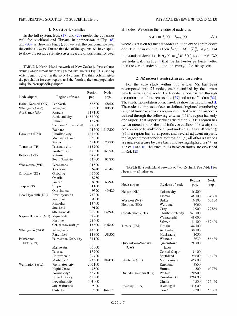
TABLE I. North Island network of New Zealand. First columndefines which airport (with designated label used in Fig. 1) is used bywhich regions, given in the second column. The third column givesthe population for each region, and the fourth is the total populationusing the corresponding airport.

Region NodeNode airport Regions of node pop. pop.

Kaitai-Kerikeri (KK) Far North 58 500 58 500Whangarei (WR) Whangarei 80 500 80 500Auckland (AK) Kaipara 1 19 150

Auckland city 1 486 000Hauraki 18 750Thames-Coromandal* 27 000Waikato 64 300 1 615 200

Hamilton (HM) Hamilton city 1 45 600Matamata-Piako 32 000Waipa 46 100 2 23 700

Tauranga (TR) Tauranga city 1 15 700Western BOP 45 800 161 500

Rotorua (RT) Rotorua 68 900South Waikato 22 900 91 800

Whakatane (WK) Whakatane 34 500Kawerau 6940 41 440

Gisborne (GB) Gisborne 46 600Opotiki 8950Wairoa 8350 63 900

Taupo (TP) Taupo 34 100Otorohanga 9320 43 420

New Plymouth (NP) New Plymouth 73 800Waitomo 9630Ruapehu 13 400Stratford 9170Sth. Taranaki 26 900 132 900

Napier-Hastings (NH) Napier city 57 800Hastings 75 500Centrl Hawkesbay* 13 500 146 800

Whanganui (WG) Whanganui 43 500Rangitikei 14 800 58 300

Palmerston Palmerston Nrth. city 82 100Nrth. (PN)

Manawatu 30 000Tararua 17 700Horowhenua 30 700Masterton* 23 500 184 000

Wellington (WL) Wellington city 200 100Kapiti Coast 49 800Porirua city* 52 700Upperhutt city 41 500Lowerhutt city 103 000Sth. Wairarapa 9420Carterton 7650 464 170

all nodes. We define the residue of node j as

j (t) = Ij (t) − Inum,j(t), (A1)

where Ij (t) is either the first-order solution or the zeroth-orderone. The mean residue is then (t) = M−1 ∑M

j=1 j (t), and

the standard deviation is σ (t) =√

M−1∑

j ( j − )2. We

see holistically in Fig. 4 that the first-order performs betterthan the zeroth-order solution, on average, for this system.

2. NZ network construction and parameters

For the case study within this article, NZ has beenrecomposed into 23 nodes, each identified by the airportwhich services the node. Each node is constructed througha combination of the census data [29] and air traffic data [32].The explicit population of each node is shown in Tables I and II.The node is composed of census defined “regions” (numbering66), and how each census region is billeted to which airport isdefined through the following criteria: (1) if a region has onlyone airport, that airport services the region; (2) If a region hastwo or more airports, the total influx or outflux of those airportsare combined to make one airport node (e.g., Kaitai-Kerikeri);(3) if a region has no airports, and several adjacent airports,the largest airport services that region; (4) all other situationsare made on a case by case basis and are highlighted via “*” inTables I and II. The travel rates between nodes are describedin Ref. [23].

TABLE II. South Island network of New Zealand. See Table I fordiscussion of columns.

Region NodeNode airport Regions of node pop. pop.

Nelson (NL) Nelson city 46 200Tasman 48 100 94 300

Westport (WS) Buller 10 100 10 100Hokitika (HK) Westland 8960

Grey 13 900 22 860Christchurch (CH) Christchurch city 367 700

Waimakariri 48 600Selwyn 41 100 457 400

Timaru (TM) Timaru 44 700Ashburton 30 100Mackenzie 4050Waimate 7630 86 480

Queenstown-Wanaka Queenstown 28 700(QW) lakes

Central Otago 184 00Southland 29 600 76 700

Blenheim (BL) Marlborough 45 600Kaikoura 3850Hurunui 11 300 60 750

Dunedin-Oamaru (DO) Waitaki 20 900Dunedin city 126 000Clutha 17 550 164 450

Invercagill (IN) Invercagill 53 000Gore* 12 300 65 300

032713-7

LLOYD P. SANDERS et al. PHYSICAL REVIEW E 88, 032713 (2013)

[1] W. O. Kermack and A. G. McKendrick, Proc. R. Soc. A: Math.Phys. Eng. Sci. 115, 700 (1927).

[2] H. W. Hethcote, in Three Basic Epidemiological Models,Applied Mathematical Ecology Vol. 18 (Springer, Berlin, 1989),pp. 119–142.

[3] K. M. E. Turner, E. J. Adams, N. Gay, A. C. Ghani, C. Mercer,and W. J. Edmunds, Theor. Biol. Med. Modell. 3, 3 (2006).

[4] J. Llibre and C. Valls, J. Math. Anal. Appl. 344, 574 (2008).[5] P. Das, Z. Mukandavire, C. Chiyaka, A. Sen, and D. Mukherjee,

Dif. Eqs. Dyn. Syst. 17, 393 (2010).[6] V. Mendez, D. Campos, and W. Horsthemke, Phys. Rev. E 86,

011919 (2012).[7] D. T. Gillespie, Annu. Rev. Phys. Chem. 58, 35 (2007).[8] M. J. Keeling and J. V. Ross, J. R. Soc. Interface 5, 171 (2008).[9] M. E. J. Newman, SIAM Rev. 45, 167 (2003).

[10] O. Woolley-Meza, C. Thiemann, D. Grady, J. J. Lee, H. Seebens,B. Blasius, and D. Brockmann, Eur. Phys. J. B 84, 589 (2011).

[11] J. P. Bagrow and Y.-R. Lin, PloS One 7, e37676 (2012).[12] D. Brockmann, in Reviews of Nonlinear Dynamics and Com-

plexity, edited by H. G. Schuster (Wiley-VCH Verlag GmbH,Weinheim, Germany, 2009), pp. 1–24.

[13] I. Hanski, Nature (London) 396, 41 (1998).[14] B. Grenfell and J. Harwood, Trends Ecol. Evolution 12, 395

(1997).[15] H. Lund, L. Lizana, and I. Simonsen, J. Stat. Phys. 151, 367

(2013).[16] V. Colizza and A. Vespignani, Phys. Rev. Lett. 99, 148701

(2007).[17] R. Parshani, S. Carmi, and S. Havlin, Phys. Rev. Lett. 104,

258701 (2010).[18] P. Van Mieghem and R. van de Bovenkamp, Phys. Rev. Lett.

110, 108701 (2013).[19] S. C. Ferreira, C. Castellano, and R. Pastor-Satorras, Phys. Rev.

E 86, 041125 (2012).[20] F. Arrigoni and A. Pugliese, J. Math. Biol. 45, 419 (2002).[21] F. Ball, Math. Biosci. 156, 41 (1999).[22] In Ref. [2] the analytical solution of the SIS model with birth and

death is provided. This solution can be used instead of Eq. (3)to yield an approximation to the temporal network dynamicsfollowing the derivation used here.

[23] The air transport rates are calculated from the worldwide airtraffic data provided by Ref. [32], taken the same year as theSubnational census data of NZ [29]. We have used the average

number of available seats (from the total average flights) perday as the measure of the number of people commuting betweentwo airport nodes in the NZ network. The travel weight ωi←j

is therefore the people leaving city j as a fraction of Nj . Wehave also removed all international connections to and from NZairports.

[24] J. J. Sakurai, Modern Quantum Mechanics (Revised Edition),1st ed. (Addison-Wesley, Reading, MA, 1993).

[25] M. Abramowitz and I. A. Stegun, Handbook of MathematicalFunctions with Formulas, Graphs, and Mathematical Tables,9th ed. (Dover, New York, 1972).

[26] Using an eigenvalue approach allows us to numerically cal-culate �I (t) at any desired (short) time without the need tointroduce a time step, as needed for instance in a Runge-Kuttaapproach.

[27] For the case of different infectivity and recovery rates for thedifferent cities, the matrix χ is replaced by a diagonal matrixwith elements χi . For this case χ and � do not commutein general, but the Baker-Campbell-Hausdorff formula stillapplies. This formula then requires us to evaluate a set ofcommutation relations in order to get an explicit expressionfor �I (t).

[28] Using the Gershgorin circle theorem [35] for diagonally domi-nant square matrices, we find that the eigenvalues of � in Eq. (20)have the following boundaries: −2 maxk Sk � λ � 0, where Sk

defines the sum of rates away from node k, Sk = ∑j �=k ωj←k , or

the sum of the column K of �.[29] Statistics New Zealand, “Subnational Populations Estimates:

At 30 June 2011, http://www.stats.govt.nz/browse_for_stats/population/estimates_and_projections/SubnationalPopulationEstimates_HOTPJun11/Commentary.aspx (2011) [online;accessed 4 April 2013].

[30] The transport rates we use [32] satisfy the detailed balancecondition, as required for the validity of Eq. (17).

[31] We consider travel to and from the Chatham islands to beinternational travel and it is therefore omitted.

[32] OAG, “Air Traffic Data”, http://www.oag.com (2011) [Dataretrieved 3 February 2011].

[33] L. Hufnagel, D. Brockmann, and T. Geisel, Proc. Natl. Acad.Sci. USA 101, 15124 (2004).

[34] R. Levins, Bull. Entomol. Soc. Am. 15, 237 (1969).[35] S. Gerschgorin, Izv. Akad. Nauk. USSR Otd. Fiz.-Mat. Nauk 7,

749 (1931).

032713-8