performance of reynolds averaged navier-stokes …...performance of reynolds averaged navier-stokes...

Performance of Reynolds Averaged Navier-Stokes

Models in Predicting Separated Flows: Study of the

Hump Flow Model Problem

Daniele Cappelli ∗

Ecole Nationale Superieure de l’Aronautique et de l’Espace, Toulouse, France

Nagi N. Mansour †

NASA Ames Research Center, Moffett-Field, CA

Separation can be seen in most aerodynamic flows, but accurate prediction of separatedflows is still a challenging problem for computational fluid dynamics (CFD) tools. Thebehavior of several Reynolds Averaged Navier-Stokes (RANS) models in predicting theseparated flow over a wall-mounted hump is studied. The strengths and weaknesses of themost popular RANS models (Spalart-Allmaras, k-ε, k-ω, k-ω-SST) are evaluated using theopen source software OpenFOAM. The hump flow modeled in this work has been docu-mented in the 2004 CFD Validation Workshop on Synthetic Jets and Turbulent SeparationControl. Only the baseline case is treated; the slot flow control cases are not considered inthis paper. Particular attention is given to predicting the size of the recirculation bubble,the position of the reattachment point, and the velocity profiles downstream of the hump.

Nomenclature

c Chord of the humpC1 Coefficient of the production term of ε for the k − ε modelC2 Coefficient of the dissipation term of ε for the k − ε modelCf Skin friction coefficientCµ Coefficient of eddy viscosity for the k − ε modelk Turbulent kinetic energyM Mach numberRec Reynolds number based on the chord of the humpS Outward-pointing face area vectorSij Rate-of-strain tensort Timeu Scalar component of velocityu Velocity vectorU∞ Asymptotic velocityx Space vectorα Coefficient of the production term of ω for the k − ω modelαω Coefficient of the viscous term of the ω equationβ Coefficient of the dissipation term of ω in the k − ω modelε Rate of dissipation of turbulent kinetic energyω Specific rate of dissipation of turbulent kinetic energyσε Coefficient of the viscous term in the ε equationρ Densityν Kinematic viscosity

∗Student intern, STIEP, NASA Ames Research Center; Double Master degrees student, SUPAERO - Politecnico di Milano†Chief Division Scientist, NASA Advanced Supercomputing Division, AIAA Associate Fellow

1 of 26

American Institute of Aeronautics and Astronautics

https://ntrs.nasa.gov/search.jsp?R=20130001741 2020-04-22T13:31:03+00:00Z

νt Turbulent kinematic viscosityνeff Effective viscosity (ν + νt)

I. Introduction

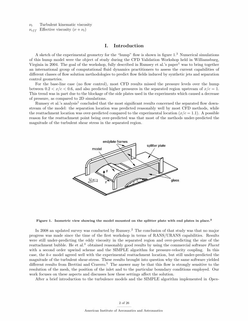
A sketch of the experimental geometry for the “hump” flow is shown in figure 1.3 Numerical simulationsof this hump model were the object of study during the CFD Validation Workshop held in Williamsburg,Virginia in 2004. The goal of the workshop, fully described in Rumsey et al.’s paper1 was to bring togetheran international group of computational fluid dynamics practitioners to assess the current capabilities ofdifferent classes of flow solution methodologies to predict flow fields induced by synthetic jets and separationcontrol geometries.

For the base-line case (no flow control), most CFD results missed the pressure levels over the humpbetween 0.2 < x/c < 0.6, and also predicted higher pressures in the separated region upstream of x/c = 1.This trend was in part due to the blockage of the side plates used in the experiments which caused a decreaseof pressure, as compared to 2D simulations.

Rumsey et al.’s analysis1 concluded that the most significant results concerned the separated flow down-stream of the model: the separation location was predicted reasonably well by most CFD methods, whilethe reattachment location was over-predicted compared to the experimental location (x/c = 1.1). A possiblereason for the reattachment point being over-predicted was that most of the methods under-predicted themagnitude of the turbulent shear stress in the separated region.

Figure 1. Isometric view showing the model mounted on the splitter plate with end plates in place.3

In 2008 an updated survey was conducted by Rumsey.2 The conclusion of that study was that no majorprogress was made since the time of the first workshop in terms of RANS/URANS capabilities. Resultswere still under-predicting the eddy viscosity in the separated region and over-predicting the size of thereattachment bubble. He et al.4 obtained reasonably good results by using the commercial software Fluentwith a second order upwind scheme and the SIMPLE algorithm for pressure-velocity coupling. In thiscase, the k-ε model agreed well with the experimental reattachment location, but still under-predicted themagnitude of the turbulent shear-stress. These results brought into question why the same software yieldeddifferent results from Brettini and Cravero.5 The answer may be that this flow is strongly sensitive to theresolution of the mesh, the position of the inlet and to the particular boundary conditions employed. Ourwork focuses on these aspects and discusses how these settings affect the solution.

After a brief introduction to the turbulence models and the SIMPLE algorithm implemented in Open-

2 of 26


FOAM,a we show our results for the baseline caseb by using 4 different turbulence models (Spalart-Allmaras,k-ε, k-ω, k-ω-SST ) and analyze the weaknesses and strengths of each RANS model. The effects that theposition of the inlet, the boundary condition on the upper wall, and the resolution of the mesh have on thehump-flow will be discussed as well.

II. RANS methods in OpenFOAM

The complete implementation of the algorithm can be found in the source code of the simpleFoam solverprovided with OpenFOAM (directory simpleFoam)c. In the appendix, we report some lines of code wherethe momentum equations and the equations for k, ε and ω are implemented. The equation for momentum,which is defined in the file UEqn.H , is:

uj∂uixj− ∂

∂xj

[νeff

(∂ui∂xj

+∂uj∂xi

)]= − ∂p

∂xi(1)

The RANS equation for turbulent kinetic energy, k, is:

∂k

∂t+ uj

∂k

∂xj− ∂

∂xj

[(νeff

)∂k

∂xj

]= νT

∂ui∂xj

(∂ui∂xj

+∂uj∂xi

)− ε (2)

While the equation for dissipation, ε, is:

∂ε

∂t+ uj

∂ε

∂xj− ∂

∂xj

[(ν +

νTσε

)∂ε

∂xj

]= C1

ε

kνT∂ui∂xj

(∂ui∂xj

+∂uj∂xi

)− C2

ε2

k(3)

By using the following definition of turbulent viscosity, νt = Cµk2

ε , we have the k − ε model. The firsttransported variable is k, the second one is ε.By defining the specific dissipation ω = ε

k , as second transported variable, we have the k − ω model. Theequation used for k is the same implemented for the k − ε model, while the equation for ω becomes:

∂ω

∂t+ uj

∂ω

∂xj− ∂

∂xj

[(ν + αωνT

)∂ω

∂xj

]= α

ω

kνT∂ui∂xj

(∂ui∂xj

+∂uj∂xi

)− βω2 (4)

The eddy viscosity is then defined as νt = kω

Because of their complexity, we will not describe the equations for the models Spalart− Allmaras andk−ω−SST . Their implementation is available in the same directory where k−ε and k−ω are implementedd.For further information about OpenFOAM we reference the reader to the manual available on the Internet.8

In table 1 we list the coefficients used in OpenFOAM for the k − ε and k − ω equations.

k − ε k − ωσε 1.3 αω 0.5

C1 1.44 α 0.52

C2 1.92 β 0.072

Cµ 0.09 Cµ 0.09

Table 1. Coefficients for the k-ε and k − ω models.

III. SIMPLE Algorithm as implemented in OpenFOAM

SimpleFOAM is a steady-state solver for incompressible, turbulent flow. We recall that the Navier-Stokesequations for a single-phase flow with a constant density and viscosity are the following:

∇ · u = 0 (5)

aThe Open-FOAM version used is the 2.1.1bThe baseline does not include the plenum, since the problem of flow-control is not dealt with here.cDirectory:openfoam211/applications/solvers/incompressible/simpleFoamdopenfoam211/src/turbulenceModels/RAS

3 of 26


∇ · (uu)−∇ · (ν∇u) = −1

ρ∇p (6)

The solution of these equations is not straightforward because of the non-linear term ∇ · (uu) and becausean explicit equation for the pressure is not available. The approach used in OpenFOAM is to derive anequation for the pressure by taking the divergence of the momentum equation and substituting it in thecontinuity equation. Temporal discretization is performed using some implicit temporal scheme, such as:6∫ t+∆t

t

f(t,U(x, t))dt = (1− C)∆tf(t,U(x, t0)) + C∆tf(t,U(x, tn)) (7)

where different values of C can recover temporal schemes defined in Juretic’s thesis.6 When the momentumequation is approximated by using the equation 7, the following relationship is derived:6,7

apup = H(u)−∇p (8)

where the subscript P refers tot he center of cell P . Velocity can be rewritten as follows:

up =H(u)

aP− ∇paP

(9)

The term H(u) includes all terms apart from the pressure gradient at the new time step and the diagonalterm anPU

nP , where the subscript n represents the new time level. The continuity equation is discretized as:

∇ · u =∑f

Suf = 0 (10)

where S is outward-pointing face area vector and uf is the velocity on the face, which is obtained byinterpolating the semi-discretized form of the momentum equation (9) as follows:

uf =

(H(u)

aP

)f

−(∇paP

)f

(11)

By substituting this equation into the discretized continuity equation above, the pressure equation is derived:

∇ ·(

1

aP∇p)

= ∇ ·(H(u)

aP

)(12)

The mass flux through a cell face can be obtained by using equation 11 as follows:

F = S ·[(

H(u)

ap

)f

−(

1

aP

)(∇p)f

](13)

A. The simpleFoam application: Implementation

The SIMPLE (Semi-Implicit Method for Pressure-Linked Equations) algorithm solves the Navier-Stokesequations with an iterative procedure, which can be summed up as follows:

1. Set the boundary conditions;

2. Solve the discretized momentum equation to compute the intermediate velocity field;

3. Compute the mass fluxes at the cells faces;

4. Solve the pressure equation and apply under-relaxation;

5. Correct the mass fluxes at the cell faces;

6. Correct the velocities on the basis of the new pressure field;

7. Update the boundary conditions;

8. Repeat till convergence.

4 of 26


IV. Results

In this section, the most significant results obtained by running the hump flow configuration in Open-FOAM are presented. In order to compare our results to experimental data, the freestream Reynolds numberand Mach number were fixed according to the experiments.

A. Fluid dynamic similitude

In order to operate in the subsonic regime, the freestream velocity was chosen to be 34.0 m/s, so thatM = 0.1 The chord of our model extends from 0.0 to 1.0 m (in order to easily compare our results with thedimensionless results provided by the other works: x/c, y/c, U/U∞). This means that in order to use thesame Reynolds number as the experimental one (the Reynolds number for the baseline case is ∼ 9300001,3, 9)we have to change the value of the kinematic viscosity in the transportProperties file, as follows:

ν =U∞c

Rec=

34.0× 1.0

930000= 3.66× 10−5m2/s (14)

In the following table, we summarize the basic properties of our set up. The Reynolds number is basedon the chord length of the humpe.

c 1 m

U∞ 34 m/s

ν 3.66×10−5 m2/s

M 0.1

Rec 930 000

Table 2. Properties of our “hump flow”

B. Mesh

For our simulations, we used two different meshes: one with the inlet set at -6x/c upstream of the leadingedge of the hump, to reproduce the experiments as well as possible and a second with inlet located at -1x/cupstream of the hump, to estimate the influence of the boundary layer on the flow; the goal is to comparethe effects of the development of the boundary layer along the lower wall of our meshf. The boundarycondition on the upper wall was changed in order to study the theoretical case (no upper wall blockage) andthe experimental one: in this case, the effects of the upper wall of the wind tunnel on the flow have beentaken into account using a no-slip condition on the upper wall.

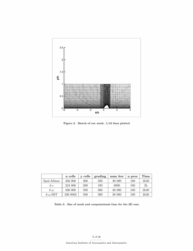
Our mesh was built by using the OpenFOAM utility blockMeshg. It was set up to be fine in the proximityof the humph. In figure 2, we show a simplified sketch of the mesh employed to run our simulations. Thegrading value defines the scale factor of our cells. A value of 100 in the y direction means that the cellsnear the lower wall are 100 times smaller than the cell close to the upper wall. In table 3 we summarize thecharacteristics of the mesh employed for the 2-D case, the number of iterations, and the computational timeto get to convergence, using 100 processors in parallel.

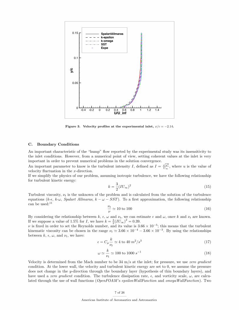
For the inlet located at -6 x/c, the length of the splitter plate has been selected to match the measuredvelocity profiles at x/c = −2.1 (see figure 3), as suggested by Blakumar.10 Only 2D simulations were run,i.e. the effects of the side plates were not taken into account. Since the mesh generated by OpenFOAM ’sblockMesh utility is 3D by default, to switch from 3D to 2D, we had to specify OpenFOAM ’s empty conditionon the side walls.

eIn the experiments the chord length was 420 mm.fThe lower wall of our mesh reproduce the splitter plate used in the experimentsgBy default, OpenFOAM handles both unstructured and structured meshes as unstructuredhThe points are scaled by using the option simpleGrading

5 of 26


x/c

y/c

-6 -4 -2 0 2 40

0.5

1

1.5

2

2.5

Figure 2. Sketch of our mesh. 1/10 lines plotted

n cells y cells grading num iter n proc Time

Spal-Allmar 336 000 300 500 30 000 100 2h30

k-ε 224 000 200 100 8000 100 2h

k-ω 336 000 500 300 30 000 100 2h30

k-ω-SST 336 0002 500 300 30 000 100 2h30

Table 3. Size of mesh and computational time for the 2D case

6 of 26


U/U_inf

y/c

-0.4 -0.2 0 0.2 0.4 0.6 0.8 1 1.2 1.40

0.05

0.1

0.15 SpalartAllmarask-epsilonk-omegaSSTExpe

Figure 3. Velocity profiles at the experimental inlet, x/c = −2.14.

C. Boundary Conditions

An important characteristic of the “hump” flow reported by the experimental study was its insensitivity tothe inlet conditions. However, from a numerical point of view, setting coherent values at the inlet is veryimportant in order to prevent numerical problems in the solution convergence.

An important parameter to know is the turbulent intensity I, defined as I =√u2

U∞, where u is the value of

velocity fluctuation in the x-direction.If we simplify the physics of our problem, assuming isotropic turbulence, we have the following relationshipfor turbulent kinetic energy:

k =3

2(IU∞)2 (15)

Turbulent viscosity, νt is the unknown of the problem and is calculated from the solution of the turbulenceequations (k-ε, k-ω, Spalart Allmaras, k − ω − SST ). To a first approximation, the following relationshipcan be used:11

νtν' 10 to 100 (16)

By considering the relationship between k, ε, ω and νt, we can estimate ε and ω, once k and νt are known.If we suppose a value of 1.5% for I, we have k = 3

2 (IU∞)2

= 0.39.ν is fixed in order to set the Reynolds number, and its value is 3.66 × 10−5; this means that the turbulentkinematic viscosity can be chosen in the range νt ' 3.66 × 10−4 − 3.66 × 10−3. By using the relationshipsbetween k, ε, ω, and νt, we have:

ε = Cµk

νt' 4 to 40 m2/s3 (17)

ω ' k

νt' 100 to 1000 s−1 (18)

Velocity is determined from the Mach number to be 34 m/s at the inlet; for pressure, we use zero gradientcondition. At the lower wall, the velocity and turbulent kinetic energy are set to 0, we assume the pressuredoes not change in the y-direction through the boundary layer (hypothesis of thin boundary layers), andhave used a zero gradient condition. The turbulence dissipation rate, ε, and vorticity scale, ω, are calcu-lated through the use of wall functions (OpenFOAM ’s epsilonWallFunction and omegaWallFunction). Two

7 of 26


different conditions have been used for the upper wall: in one case, we assume the upper wall blockage isnegligible: a symmetry plane condition is used. For the second case, in order to evaluate the effects of thewalls on the flow, we imposed a viscous wall condition (the same used for the lower wall). At the exit, wechose a zero gradient condition for all the variables, except that the pressure is forced to equal the asymptoticpressure. Since in the simpleFoam solver, psimpleFoam = ∆p

ρ , we have p = 0 at the outlet. The boundaryconditions that we have defined are summarized in tables 4 and 5.

inlet lower wall upper wall outlet

U 34 m/s 0 m/s symmetry plane zero gradient

p zero gradient zero gradient symmetry plane p = p∞

νt 3.66e-4 m2/s wall function symmetry plane zero gradient

k 0.39 m2/s2 0 m2/s2 symmetry plane zero gradient

ε 37.4 m2/s3 wall function symmetry plane zero gradient

ω 500 1/s wall function symmetry plan zero gradient

Table 4. Boundary conditions for the 2D case. Upper wall considered as a symmetry plane.

inlet lower wall upper wall outlet

U 34 m/s 0 m/s 0 m/s zero gradient

p zero gradient zero gradient zero gradient p = p∞

νt 3.66e-4 m2/s wall function wall function zero gradient

k 0.39 m2/s2 0 m2/s2 0 m2/s2 zero gradient

ε 37.4 m2/s3 wall function wall function zero gradient

ω 500 1/s wall function wall function zero gradient

Table 5. Boundary conditions for the 2D case. Upper wall considered as viscous wall.

D. Pressure

In this section the results for pressure in the 2D case are shown. In figures 4, 5, 6 and 7, the trend of pressurefor the different turbulence methods is shown as contour plots covering the entire computational domain,while in figures 8 and 9, pressure coefficients are compared to experimental data. These simulations wererun by using both 1-equation and 2-equation turbulence models, more specifically: Spalart-Allmaras i, k-ε,k-ω, k-ω-SSTj. Pressure shows how the flow is accelerated up to around the mid-chord of the hump, wherea peak magnitude of Cp is observed. A sudden drop of pressure downstream leads to a separation at aroundx/c=0.65, which corresponds to the location of the cavity slot for the controlled casesk. The exp-no-platesdata refer to the pressure coefficients measured in the absence of the end-side plates. In this case, the problemof blockage does not affect the measurements, so that the pressure is not under-predicted. In figure 8, ourcasesl are compared with experiments: all the methods are very close to the experimental results withoutplates, except k-ω-SST which over-predicts pressure. In figure 9, simulations are run by taking into accountthe effects of the upper wall, and are compared with experiments: in this case we have a slight improvementin the pressure prediction, especially for the k-ω-SST model that matches the experimental results very well.Downstream of the separation point, pressure is over predicted by Spalart Allmaras and k-ε, while k-ω andk-ω-SST provide accurate results.

iOne equation modeljTwo equation modelskIn this study the controlled case will not be studiedlIn this plot, the upper wall is treated as a symmetric plane

8 of 26


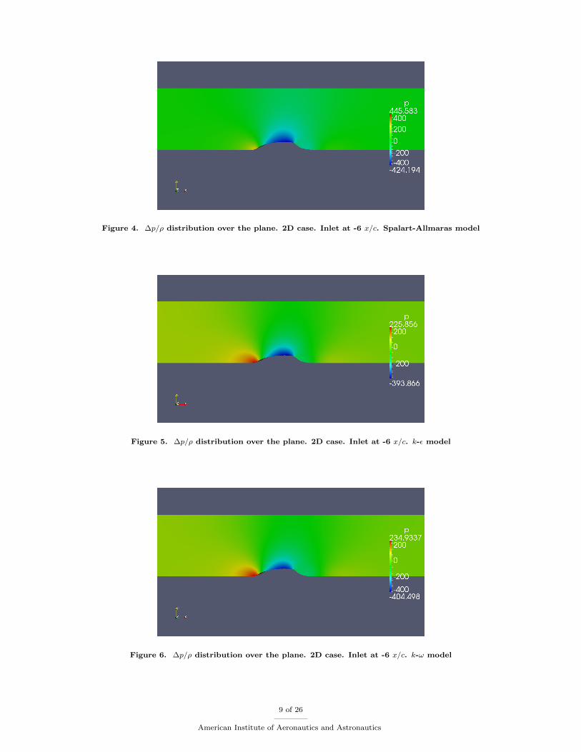
Figure 4. ∆p/ρ distribution over the plane. 2D case. Inlet at -6 x/c. Spalart-Allmaras model

Figure 5. ∆p/ρ distribution over the plane. 2D case. Inlet at -6 x/c. k-ε model

Figure 6. ∆p/ρ distribution over the plane. 2D case. Inlet at -6 x/c. k-ω model

9 of 26


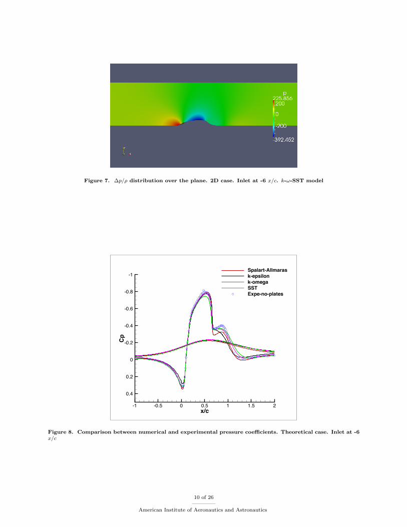
Figure 7. ∆p/ρ distribution over the plane. 2D case. Inlet at -6 x/c. k-ω-SST model

x/c

Cp

-1 -0.5 0 0.5 1 1.5 2

-1

-0.8

-0.6

-0.4

-0.2

0

0.2

0.4

Spalart-Allmarask-epsilonk-omegaSSTExpe-no-plates

Figure 8. Comparison between numerical and experimental pressure coefficients. Theoretical case. Inlet at -6x/c

10 of 26


x/c

Cp

-1 -0.5 0 0.5 1 1.5 2

-1

-0.8

-0.6

-0.4

-0.2

0

0.2

0.4

SSTSpalart-Allmarask-omegak-epsilonExpe-no-plates

Figure 9. Comparison between numerical and experimental pressure coefficients, by taking into account theeffects of the upper wall. 2D case. Inlet at -6 x/c

E. Velocity

In figures 10, 11, 12 and 13 the velocity field is shown for all turbulence models; these are 2D cases thatdo not take into account the blockage of the upper wall. In figures 14, 15, 16 and 17, velocity profiles atx/c = 0.8, x/c = 1.0, x/c = 1.1 and x/c = 1.2 are compared with experimental results (inlet located at -6x/c). Our grid origin is the beginning of the hump, so that 1.0 x/c is the last point of the hump.In the contour plots, the recirculation bubble (low speed flow marked by blue color) is visible for all of themodels. The trend of velocity is the same for all models: the flow accelerates where the pressure drops andseparates soon after. The size of the bubble may change for different models; we will discuss this aspect inthe following section.

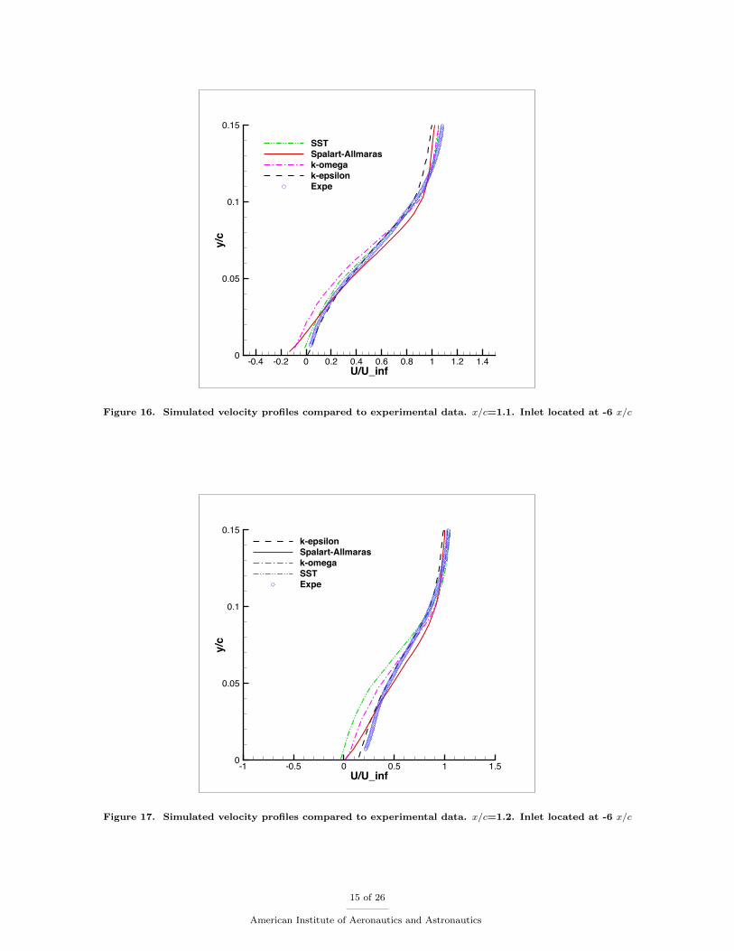
The most significant results are obtained by comparing the velocity profiles downstream of the hump.Velocity profiles are extracted in the bubble (x/c = 0.8 and x/c = 1.0), at the experimental reattachmentpoint (x/c = 1.1), and outside the bubble (x/c = 1.2). The predicted profiles match the experimental resultsvery well at all locations except x/c = 1.2 which is a critical location. As we will see in the next section,most numerical methods predict the reattachment point to be very close to x/c = 1.2, while experimentaldata suggest x/c = 1.1. Spalart-Allmaras, k − ω, and SST fail to reproduce the velocity profile correctlyat x/c = 1.2 close to the wall, while k − ε provides good results, probably because it is the most accuratemethod in predicting the position of the reattachment pointm. In figure 18 the effects of the upper wall onvelocity are shown. We can see the boundary layer developing all along the upper wall of our geometry.This is responsible for the decrease in pressure we show in figure 9. The presence of the upper wall does notaffect the bubble or the velocity profiles downstream of the hump. In figure 19 we show the velocity profilesat the critical location x/c = 1.2. The trend is very similar to the one obtained by using a symmetry planeas the boundary condition for the upper wall.

To have an idea of the accuracy of our solutions we show the velocity profiles collected by Rumsey at x/c =1.2 (figure 20). In this case, two methods predict the experimental results with a good accuracy:AZ-cobalt-des-1-3d and META-cfd++lns-3D. These are two hybrid LES/RANS methods. One of them implements theDES method (Detached Eddy Simulation), the other one implements the LNS method (Limited Numerical

mThese aspects will be discussed deeper in the next section.

11 of 26


Scales). All the other curves, obtained by using RANS models, are quite far from the experimental results:an evidence is the fact that, in proximity of the wall, u-velocities are negative, while the experimental curvepredicts positive values. This is a consequence of the fact that the RANS simulations used in the workshopover-predicted the length of the bubble, so that the location x/c=1.2 was still inside the recirculation zone.The good behavior of the k-ε method used in our simulations may be a consequence of predicting the size ofthe bubble properly.

F. Inlet located at x/c = −1

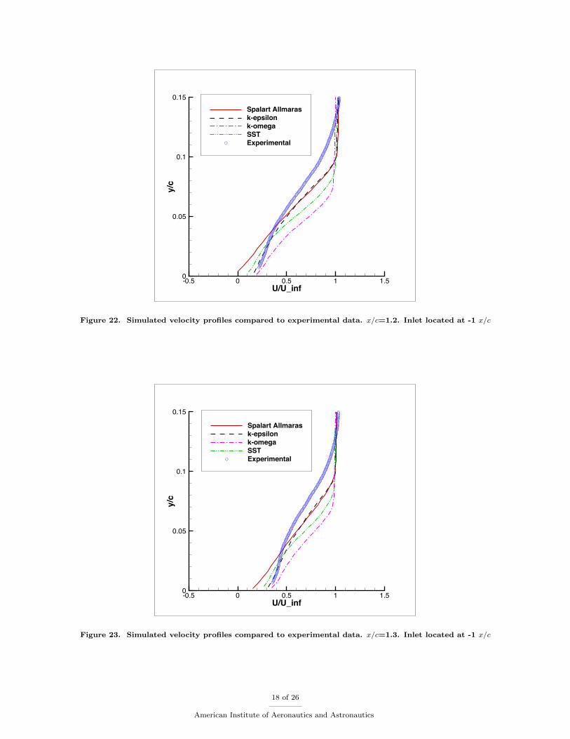
In this section we want to analyze the effects of the location of the inlet on the velocity profiles. So far,the inlet has been located at -6x/c upstream of the hump. In figures 21, 22, and 23 we show the behaviorof velocity profiles for the inlet located at -1x/c upstream of the hump. In this case the boundary layer atthe lower wall is thinner than that calculated for the inlet located -6 x/c upstream of the hump: when theflow separates, the wake remains thinner, so that if we move from the lower wall to the upper wall, we seethat the velocity profile reaches the external flow velocity faster than the experimental results. This is veryimportant, because it shows that, even if the “hump flow” is not sensitive to different inlet conditions (interms of Reynolds number and Mach number as shown by Greenblatt3 in experiments), the position of theinlet plays an important role in the accuracy of solution.

Figure 10. Zoom of velocity field in the x− y plane. 2D case. Inlet at -6 x/c. Spalart-Allmaras model

Figure 11. Zoom of velocity field in the x− y plane. 2D case. Inlet at -6 x/c. k-ε model

12 of 26


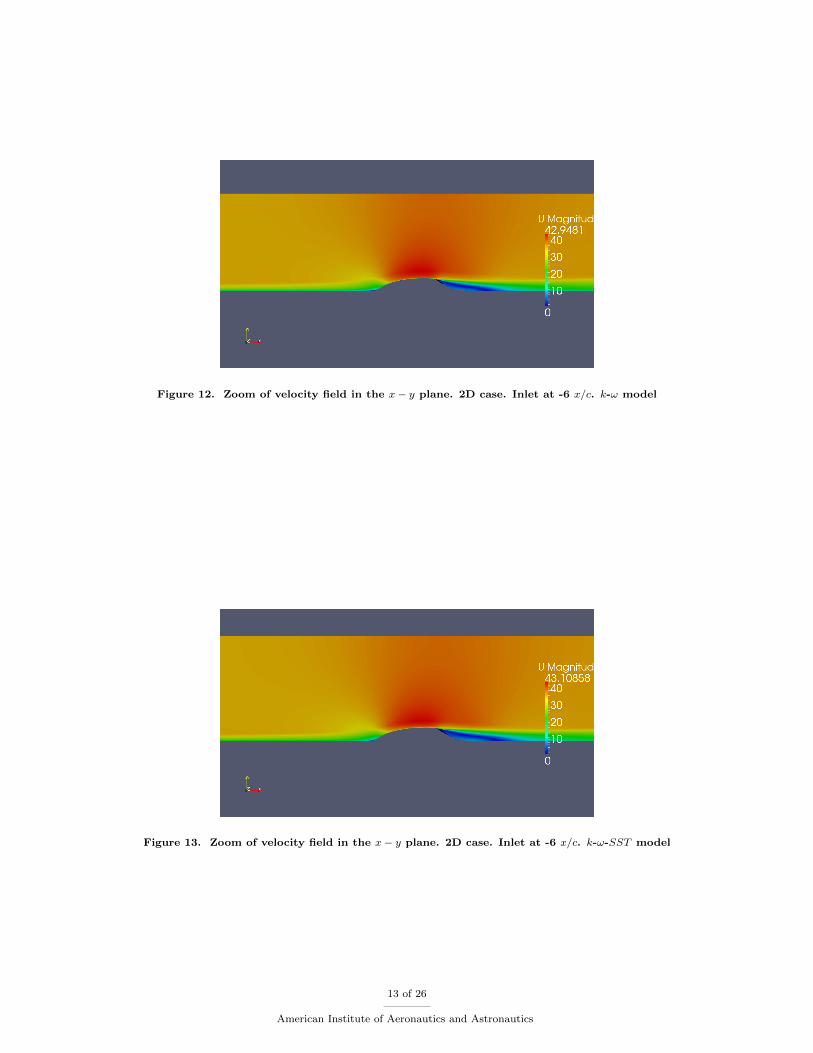
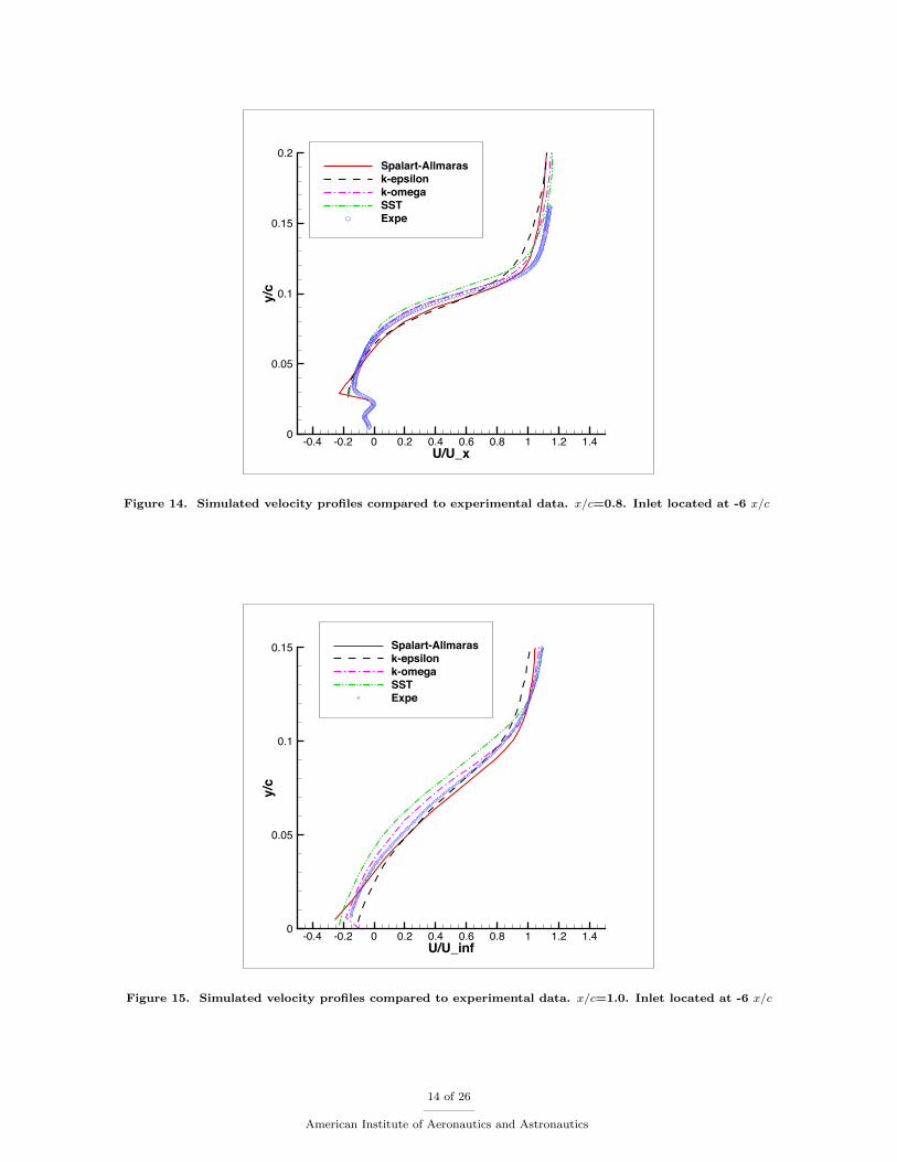
Figure 12. Zoom of velocity field in the x− y plane. 2D case. Inlet at -6 x/c. k-ω model

Figure 13. Zoom of velocity field in the x− y plane. 2D case. Inlet at -6 x/c. k-ω-SST model

13 of 26


U/U_x

y/c

-0.4 -0.2 0 0.2 0.4 0.6 0.8 1 1.2 1.40

0.05

0.1

0.15

0.2Spalart-Allmarask-epsilonk-omegaSSTExpe

Figure 14. Simulated velocity profiles compared to experimental data. x/c=0.8. Inlet located at -6 x/c

U/U_inf

y/c

-0.4 -0.2 0 0.2 0.4 0.6 0.8 1 1.2 1.40

0.05

0.1

0.15 Spalart-Allmarask-epsilonk-omegaSSTExpe


14 of 26


U/U_inf

y/c

-0.4 -0.2 0 0.2 0.4 0.6 0.8 1 1.2 1.40

0.05

0.1

0.15

SSTSpalart-Allmarask-omegak-epsilonExpe


U/U_inf

y/c

-1 -0.5 0 0.5 1 1.50

0.05

0.1

0.15k-epsilonSpalart-Allmarask-omegaSSTExpe


15 of 26


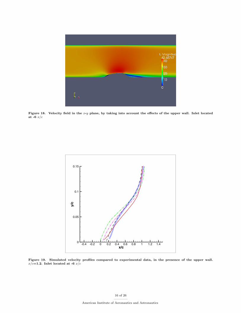
Figure 18. Velocity field in the x-y plane, by taking into account the effects of the upper wall. Inlet locatedat -6 x/c

x/c

y/c

-0.4 -0.2 0 0.2 0.4 0.6 0.8 1 1.2 1.40

0.05

0.1

0.15

Figure 19. Simulated velocity profiles compared to experimental data, in the presence of the upper wall.x/c=1.2. Inlet located at -6 x/c

16 of 26


Figure 20. Velocity profiles collected by Rumsey. x/c = 1.21

U/U_inf

y/c

-0.5 0 0.5 1 1.50

0.05

0.1

0.15Spalart Allmarask-epsilonk-omegaSSTExperimental


17 of 26


U/U_inf

y/c

-0.5 0 0.5 1 1.50

0.05

0.1

0.15

Spalart Allmarask-epsilonk-omegaSSTExperimental


U/U_inf

y/c

-0.5 0 0.5 1 1.50

0.05

0.1

0.15

Spalart Allmarask-epsilonk-omegaSSTExperimental


18 of 26


G. Recirculation zone

The size of the bubble is an important parameter for the evaluation of the accuracy of our simulations. Inorder to estimate the length of the bubble, both the separation point and the reattachment point have to beevaluated. This is possible by examining the curve of the skin friction coefficient. When the curve cuts thezero axis, the term du/dn is zero. It means that the flow is separating or reattaching. In order to get theskin friction coefficient trend, we have to compute the derivative of velocity along n. This field is not one ofthe standard outputs in the software, so we need to modify the source code of OpenFOAM by defining thisnew parameter. Once du/dn is available, we can compute Cf as:

Cf =τ

12ρU

2∞

=µ∂U∂y

12ρU

2∞

(19)

Figure 24 shows the skin friction coefficient over the hump for all the RANS models we considered. Theupper wall blockage does not affect the value of the skin friction at the lower wall. Curves are shown for bothcases (viscous wall and symmetry plane) with the inlet located at -6x/c. By identifying the points where theCf curves cut the axis, it possible to locate the separation point and the reattachment point. As we can seein table 6 and in figure 24, the separation point is accurately predicted by all the RANS models, while theonly model able to catch the exact position of reattachment is k− ε. This explains why the velocity profilesdownstream of the reattachment point are better predicted by the k − ε model as compared to the othermodels. Figures 25, 26, 27 and 28 show the size of the bubble computed with different RANS models. Thesmallest bubble is predicted by k − ε, the biggest by k − ω − SST as summarized in table 6.

x/c

Cf

-0.5 0 0.5 1 1.5-0.005

0

0.005

0.01

0.015k-epsilonk-omegaSpalart-AllmarasSSTExpe

Figure 24. Skin friction coefficient. Inlet located at x/c = −6

H. Turbulent Shear Stress

Rumsey reported that one of the parameters that can affect the prediction of the size of the bubble is theturbulent shear stress. He concluded that as long as this parameter is not predicted properly, the turbulencein the bubble can be compromised and its length and size mispredicted. After having defined the derivativesof velocity in OpenFOAM, we compute the turbulent shear stress by using Boussinesq’s hypothesis:

u′v′ = −2νtSij = −νt(∂u

∂y+∂v

∂x

)(20)

19 of 26


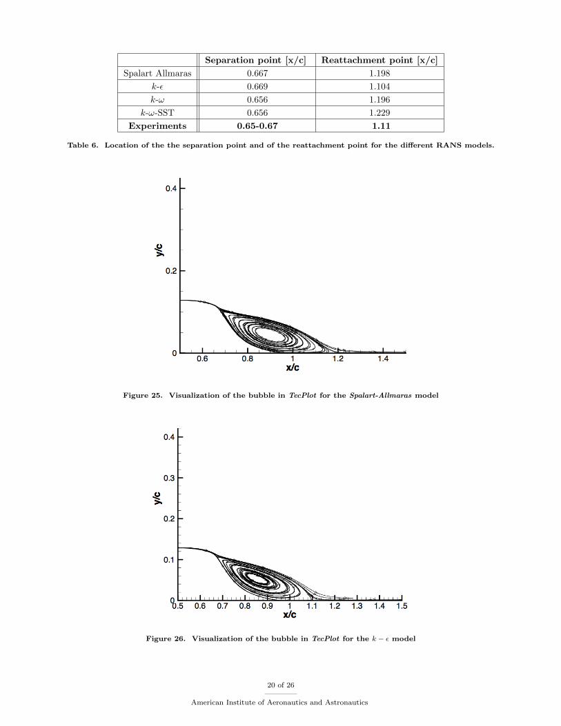
Separation point [x/c] Reattachment point [x/c]

Spalart Allmaras 0.667 1.198

k-ε 0.669 1.104

k-ω 0.656 1.196

k-ω-SST 0.656 1.229

Experiments 0.65-0.67 1.11

Table 6. Location of the the separation point and of the reattachment point for the different RANS models.

Figure 25. Visualization of the bubble in TecPlot for the Spalart-Allmaras model

Figure 26. Visualization of the bubble in TecPlot for the k − ε model

20 of 26


Figure 27. Visualization of the bubble in TecPlot for the k − ω model

Figure 28. Visualization of the bubble in TecPlot for the SST model

21 of 26


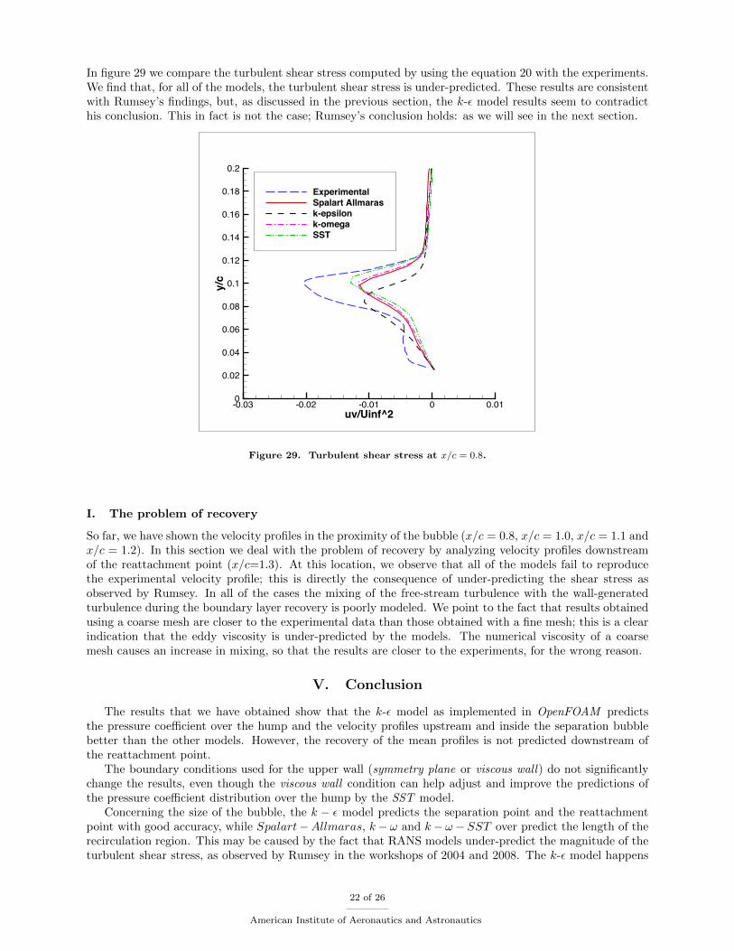
In figure 29 we compare the turbulent shear stress computed by using the equation 20 with the experiments.We find that, for all of the models, the turbulent shear stress is under-predicted. These results are consistentwith Rumsey’s findings, but, as discussed in the previous section, the k-ε model results seem to contradicthis conclusion. This in fact is not the case; Rumsey’s conclusion holds: as we will see in the next section.

uv/Uinf^2

y/c

-0.03 -0.02 -0.01 0 0.010

0.02

0.04

0.06

0.08

0.1

0.12

0.14

0.16

0.18

0.2

ExperimentalSpalart Allmarask-epsilonk-omegaSST

Figure 29. Turbulent shear stress at x/c = 0.8.

I. The problem of recovery

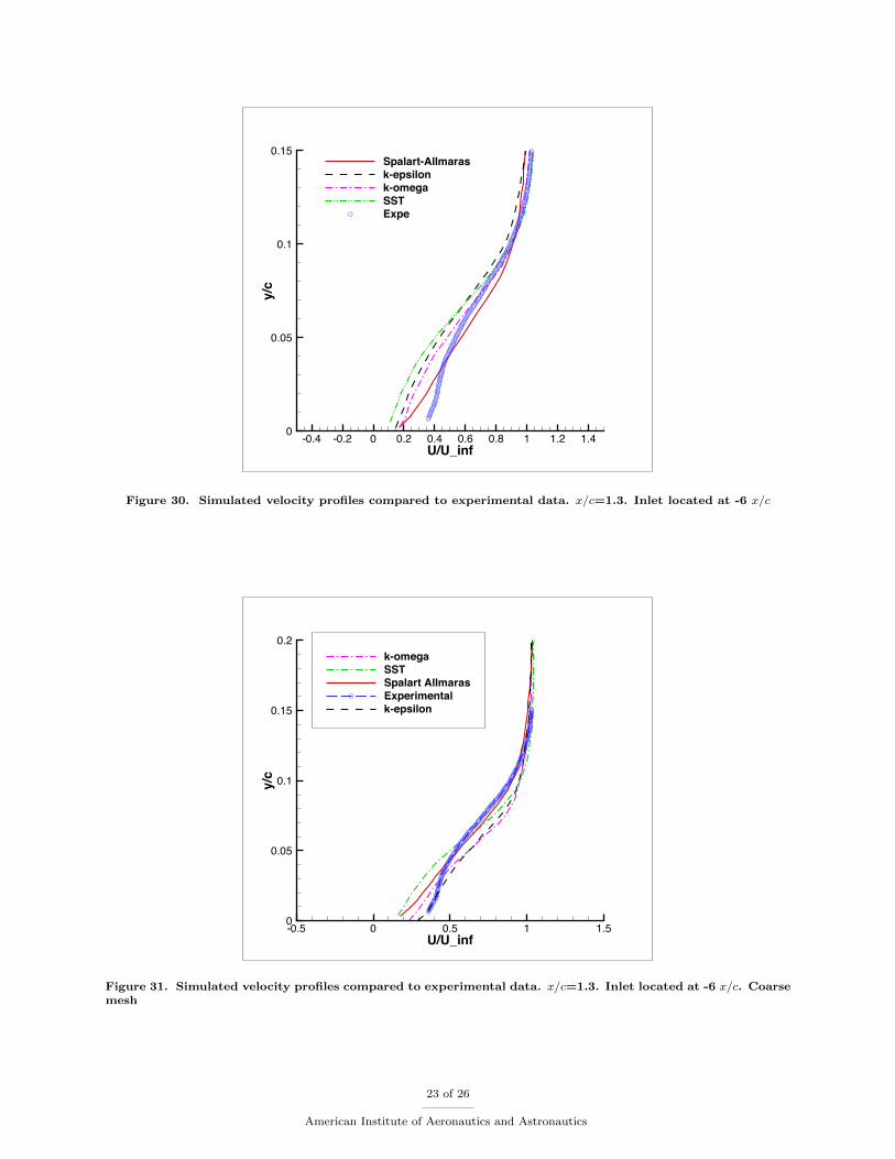
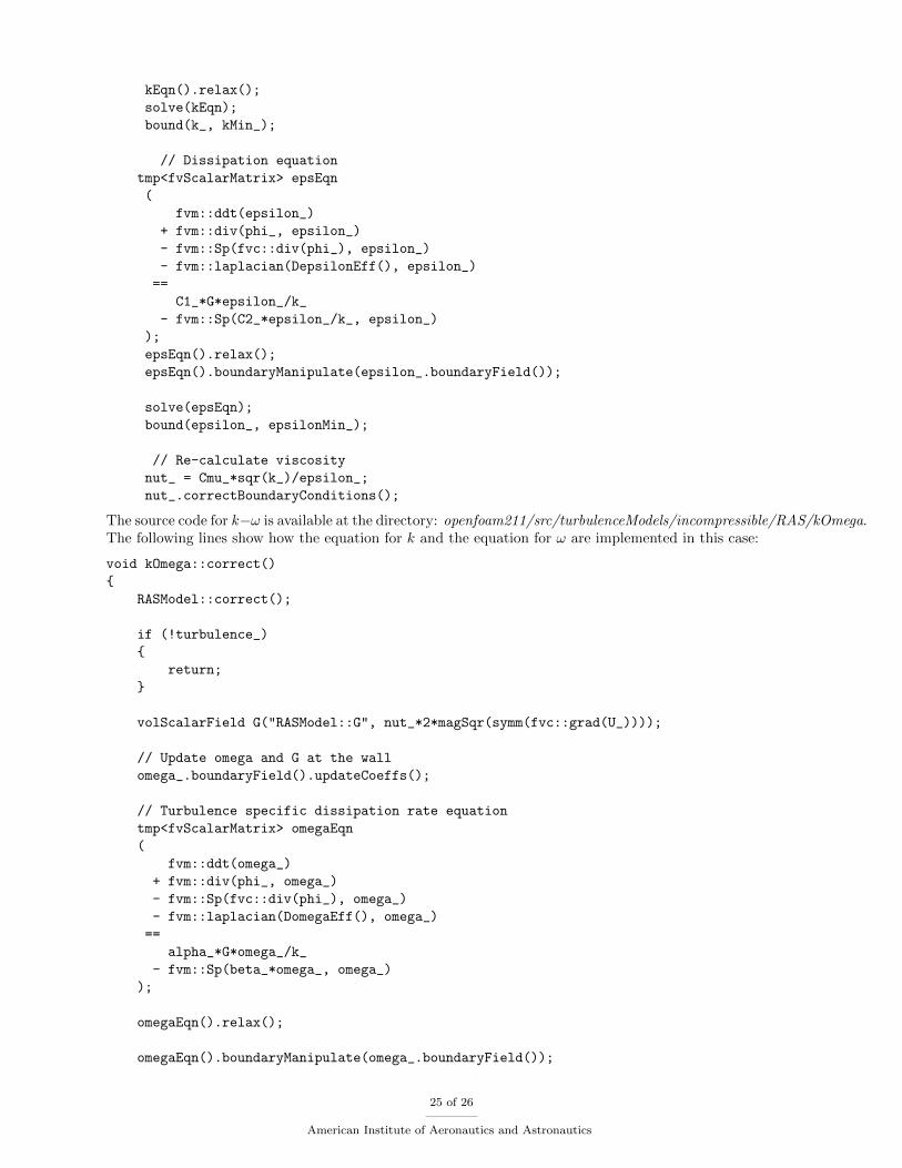
So far, we have shown the velocity profiles in the proximity of the bubble (x/c = 0.8, x/c = 1.0, x/c = 1.1 andx/c = 1.2). In this section we deal with the problem of recovery by analyzing velocity profiles downstreamof the reattachment point (x/c=1.3). At this location, we observe that all of the models fail to reproducethe experimental velocity profile; this is directly the consequence of under-predicting the shear stress asobserved by Rumsey. In all of the cases the mixing of the free-stream turbulence with the wall-generatedturbulence during the boundary layer recovery is poorly modeled. We point to the fact that results obtainedusing a coarse mesh are closer to the experimental data than those obtained with a fine mesh; this is a clearindication that the eddy viscosity is under-predicted by the models. The numerical viscosity of a coarsemesh causes an increase in mixing, so that the results are closer to the experiments, for the wrong reason.

V. Conclusion

The results that we have obtained show that the k-ε model as implemented in OpenFOAM predictsthe pressure coefficient over the hump and the velocity profiles upstream and inside the separation bubblebetter than the other models. However, the recovery of the mean profiles is not predicted downstream ofthe reattachment point.

The boundary conditions used for the upper wall (symmetry plane or viscous wall) do not significantlychange the results, even though the viscous wall condition can help adjust and improve the predictions ofthe pressure coefficient distribution over the hump by the SST model.

Concerning the size of the bubble, the k − ε model predicts the separation point and the reattachmentpoint with good accuracy, while Spalart−Allmaras, k− ω and k− ω− SST over predict the length of therecirculation region. This may be caused by the fact that RANS models under-predict the magnitude of theturbulent shear stress, as observed by Rumsey in the workshops of 2004 and 2008. The k-ε model happens

22 of 26


U/U_inf

y/c

-0.4 -0.2 0 0.2 0.4 0.6 0.8 1 1.2 1.40

0.05

0.1

0.15Spalart-Allmarask-epsilonk-omegaSSTExpe


U/U_inf

y/c

-0.5 0 0.5 1 1.50

0.05

0.1

0.15

0.2k-omegaSSTSpalart AllmarasExperimentalk-epsilon

Figure 31. Simulated velocity profiles compared to experimental data. x/c=1.3. Inlet located at -6 x/c. Coarsemesh

23 of 26


to match the shear stress at the location that affects the size of the bubble.Even if the hump-flow is considered insensitive to inlet conditions in terms of the Reynolds and Mach

numbers, the development of the boundary layer upstream of the hump strongly affects the velocity profilesdownstream. This is evidenced by the fact that by moving the inlet face of our mesh from x/c = −6 tox/c = −1, the field of velocity computed downstream of the model changes substantially.

Particular attention has to be paid to the resolution of the mesh, which plays a very important role inthe accuracy of results. More specifically, since we are interested in the derivatives of velocity (skin frictioncoefficient) and in the pressure distribution over the hump, the mesh has to be very fine close to the lowerwall. In our work, we have scaled the mesh so that the points in proximity of the hump are 300 or 500 timessmaller than in the free stream. A mesh that does not satisfy these requirements does not provide accuratevalues of pressure and skin friction or can provide good results for the wrong reason (problem of recovery ofvelocity).

Finally, our results are consistent with those obtained by He et al,4 who used the commercial softwareFluent. But predictions could be different from other results, even when computed using the same software,because of the great sensitivity of the solution to all of the variables discussed in the paper.

Appendix

The equation for momentum is defined in the file UEqn.H

tmp<fvVectorMatrix> UEqn

(

fvm::div(phi, U)

+ turbulence->divDevReff(U)

==

sources(U)

);

UEqn().relax();

sources.constrain(UEqn());

solve(UEqn() == -fvc::grad(p));

...

tmp<fvVectorMatrix> kEpsilon::divDevReff(volVectorField& U) const

{

return

(

- fvm::laplacian(nuEff(), U)

- fvc::div(nuEff()*dev(T(fvc::grad(U))))

);

}

The source code for k − ε model is in the directory openfoam211/src/turbulenceModels/RAS/kEpsilon.Here we report the lines of code where the equations for k and ε are implemented:

// Turbulent kinetic energy equation

tmp<fvScalarMatrix> kEqn

(

fvm::ddt(k_)

+ fvm::div(phi_, k_)

- fvm::Sp(fvc::div(phi_), k_)

- fvm::laplacian(DkEff(), k_)

==

G

- fvm::Sp(epsilon_/k_, k_)

);

24 of 26


kEqn().relax();

solve(kEqn);

bound(k_, kMin_);

// Dissipation equation

tmp<fvScalarMatrix> epsEqn

(

fvm::ddt(epsilon_)

+ fvm::div(phi_, epsilon_)

- fvm::Sp(fvc::div(phi_), epsilon_)

- fvm::laplacian(DepsilonEff(), epsilon_)

==

C1_*G*epsilon_/k_

- fvm::Sp(C2_*epsilon_/k_, epsilon_)

);

epsEqn().relax();

epsEqn().boundaryManipulate(epsilon_.boundaryField());

solve(epsEqn);

bound(epsilon_, epsilonMin_);

// Re-calculate viscosity

nut_ = Cmu_*sqr(k_)/epsilon_;

nut_.correctBoundaryConditions();

The source code for k−ω is available at the directory: openfoam211/src/turbulenceModels/incompressible/RAS/kOmega.The following lines show how the equation for k and the equation for ω are implemented in this case:

void kOmega::correct()

{

RASModel::correct();

if (!turbulence_)

{

return;

}

volScalarField G("RASModel::G", nut_*2*magSqr(symm(fvc::grad(U_))));

// Update omega and G at the wall

omega_.boundaryField().updateCoeffs();

// Turbulence specific dissipation rate equation

tmp<fvScalarMatrix> omegaEqn

(

fvm::ddt(omega_)

+ fvm::div(phi_, omega_)

- fvm::Sp(fvc::div(phi_), omega_)

- fvm::laplacian(DomegaEff(), omega_)

==

alpha_*G*omega_/k_

- fvm::Sp(beta_*omega_, omega_)

);

omegaEqn().relax();

omegaEqn().boundaryManipulate(omega_.boundaryField());

25 of 26


solve(omegaEqn);

bound(omega_, omegaMin_);

// Turbulent kinetic energy equation

tmp<fvScalarMatrix> kEqn

(

fvm::ddt(k_)

+ fvm::div(phi_, k_)

- fvm::Sp(fvc::div(phi_), k_)

- fvm::laplacian(DkEff(), k_)

==

G

- fvm::Sp(Cmu_*omega_, k_)

);

kEqn().relax();

solve(kEqn);

bound(k_, kMin_);

// Re-calculate viscosity

nut_ = k_/omega_;

nut_.correctBoundaryConditions();

}

// * * * * * * * * * * * * * * * * * * * * * * * * * * * * * * * * * * * * * //

Acknowledgments

The authors would like to thank the following people for the help they provided: Susheel Sekhar NPPFellow, NASA ARC, Jean Lachaud, ARC, University of California - Santa Cruz, and Julien De MuelenaerePhD student at Stanford University.

References

1C.L. Rumsey and T.B. Gatski and W.L. Sellers and V.N. Vatsa and S.A. Viken, Summary of the 2004 CFD ValidationWorkshop on Synthetic Jets and Turbulent Separation Control , Nasa Langley Research Center, AIAA 2005-1270, 2005.

2Christopher L. Rumsey Successes and Challenges for Flow Control Simulations , Nasa Langley Research Center - AIAA2008-4311, 2008.

3David Greenblatt and Keith B. Paschal and Chung-Sheng Yao and Jerome Harris and Norman Schaeffler and Anthony E.Washburn, A Separation Control CFD Validation Test Case. Part 1, AIAA 2004-2220, 2004.

4Chuan He and Thomas C. Corke , Numerical and Experimental Analysis of Plasma Flow Control Over a Hump Model ,University of Notre Drame, IN, 2007.

5Bettini, C. and Cravero, C, Computational Analysis of Flow Separation Control for the Flow over a Wall-MountedHumpUsing a synthetic Jet, AIAA Paper 2007-0516, 2007.

6Franjo Juretic, Error analysis in Finite Volume CFD, PhD Thesis, Imperial College, 2004.7Jasak H., Error analysis and estimation for the Finite Volume method with applications to fluid flows, PhD Thesis,

Imperial College, 1996.8OpenFOAM foundation, www.openfoam.org/doc , User Guide, 2012.9http://cfdval2004.larc.nasa.gov/ , CFD Validation of Synthetic Jets and Turbulent Separation Control , NASA Langley

Research Center.10P.Balakumar, Computations of Flow over a Hump Model Using Higher Order Method with Turbulence Modeling , Nasa

Langley Research Center, AIAA 2004-2220, 2004.11Platteeuw P.D.A, Application of the Probabilistic Collocation method to uncertainty in turbulence models , M. Sc. THesis,

2008

26 of 26


performance of reynolds averaged navier-stokes …...performance of reynolds averaged navier-stokes...

Documents