pdfs.semanticscholar.org stochastic processes, theory for applications solutions to selected...
TRANSCRIPT

1
Stochastic Processes,Theory for Applications
Solutions to Selected Exercises
R.G.GallagerOctober 5, 2014
The complete set of solutions is available to instructors teaching this course. ContactCambridge Press at www.Cambridge.org.
The solutions here occasionally refer to theorems, corollaries, and lemmas in the text. Thenumbering of theorems etc. in the text is slightly di↵erent from that of the draft of Chapters1-3 on my web site. Theorems, corollaries, lemmas, definitions, and examples are numberedseparately on the web site, but numbered collectively in the text. Thus students using theweb site must use some care in finding the theorem, etc. that is being referred to.
The author gratefully acknowleges the help of Shan-Yuan Ho, who has edited many of thesesolutions, and of a number of teaching assistants, particulartly Natasha Blitvic and MinaKarzand, who wrote earlier drafts of solutions. Thanks are also due to Kluwer AcademicPress for permission to use a number of exercises that also appeared in Gallager, ‘DiscreteStochastic Processes,’ Kluwer, 1995. The original solutions to those exercises were preparedby Shan-Yuan Ho, but changed substantially here by the author both to be consistent withthe new text and occasionally for added clarity.
The author will greatly appreciate being notified of typos, errors, di↵erent approaches, andlapses in clarity at [email protected].

2 APPENDIX A. SOLUTIONS TO EXERCISES
A.1 Solutions for Chapter 1
Exercise 1.2: This exercise derives the probability of an arbitrary (non-disjoint) union of events, derivesthe union bound, and derives some useful limit expressions.
a) For 2 arbitrary events A1 and A2, show that
A1
[A2 = A1
[(A2�A1), (A.1)
where A2�A1 = A2Ac1. Show that A1 and A2 � A1 are disjoint. Hint: This is what Venn diagrams were
invented for.
Solution: Note that each sample point ! is in A1 or Ac1, but not both. Thus each ! is in
exactly one of A1, Ac1A2 or Ac
1Ac2. In the first two cases, ! is in both sides of (A.1) and in
the last case it is in neither. Thus the two sides of (A.1) are identical. Also, as pointed outabove, A1 and A2 � A1 are disjoint. These results are intuitively obvious from the Venndiagram,
�⇢
⇠⇡
�⇢
⇠⇡6
⇥⇥⇥�
BBBM6
?
AAU
��↵
A1 A2
A1A2 A2Ac1 = A2�A1A1A
c2
b) For any n � 2 and arbitrary events A1, . . . , An, define Bn = An �Sn�1
i=1 Ai. Show that B1, B2, . . . are
disjoint events and show that for each n � 2,Sn
i=1 Ai =Sn
i=1 Bi. Hint: Use induction.
Solution: Let B1 = A1. From (a) B1 and B2 are disjoint and (from (A.1)), A1S
A2 =B1S
B2. Let Cn =Sn
i=1 Ai. We use induction to prove that Cn =Sn
i=1 Bi and that theBn are disjoint. We have seen that C2 = B1
SB2, which forms the basis for the induction.
We assume that Cn�1 =Sn�1
i=1 Bi and prove that Cn =Sn
i=1 Bi.
Cn = Cn�1
[An = Cn�1
[AnCc
n�1
= Cn�1
[Bn =
[n
i�1Bi.
In the second equality, we used (A.1), letting Cn�1 play the role of A1 and An play the roleof A2. From this same application of (A.1), we also see that Cn�1 and Bn = An�Cn�1 aredisjoint. Since Cn�1 =
Sn�1i=1 Bi, this also shows that Bn is disjoint from B1, . . . , Bn�1.
c) Show that
Prn[1
n=1An
o= Pr
n[1
n=1Bn
o=X1
n=1Pr{Bn} .
Solution: If ! 2S1
n=1 An, then it is in An for some n � 1. Thus ! 2Sn
i=1 Bi, and thus! 2
S1n=1 Bn. The same argument works the other way, so
S1n=1 An =
S1n=1 Bn. This
establishes the first equality above, and the second is the third axiom of probability.
d) Show that for each n, Pr{Bn} Pr{An}. Use this to show that
Prn[1
n=1An
oX1
n=1Pr{An} .

A.1. SOLUTIONS FOR CHAPTER 1 3
Solution: Since Bn = An �Sn�1
i=1 Ai, we see that ! 2 Bn implies that ! 2 An, i.e., thatBn ✓ An. From (1.5), this implies that Pr{Bn} Pr{An} for each n. Thus
Prn[1
n=1An
o=X1
n=1Pr{Bn}
X1
n=1Pr{An} .
e) Show that Pr�S1
n=1 An
= limn!1 Pr
�Sni=1 Ai
. Hint: Combine (c) and (b). Note that this says that
the probability of a limit is equal to the limit of the probabilities. This might well appear to be obvious
without a proof, but you will see situations later where similar appearing interchanges cannot be made.
Solution: From (c),
Prn[1
n=1An
o=X1
n=1Pr{Bn} = lim
k!1
Xk
n=1Pr{Bn} .
From (b), however,
Xk
n=1Pr{Bn} = Pr
(k[
n=1
Bn
)= Pr
(k[
n=1
An
).
Combining the first equation with the limit in k of the second yields the desired result.
f) Show that Pr�T1
n=1 An
= limn!1 Pr
�Tni=1 Ai
. Hint: Remember De Morgan’s equalities.
Solution: Using De Morgans equalities,
Pr
( 1\n=1
An
)= 1� Pr
( 1[n=1
Acn
)= 1� lim
k!1Pr
(k[
n=1
Acn
)
= limk!1
Pr
(k\
n=1
An
).
Exercise 1.4: Consider a sample space of 8 equiprobable sample points and let A1, A2, A3 be threeevents each of probability 1/2 such that Pr{A1A2A3} = Pr{A1}Pr{A2}Pr{A3}.
a) Create an example where Pr{A1A2} = Pr{A1A3} = 14 but Pr{A2A3} = 1
8 . Hint: Make a table with a
row for each sample point and a column for each of the above 3 events and try di↵erent ways of assigning
sample points to events (the answer is not unique).
Solution: Note that exactly one sample point must be in A1, A2, and A3 in order to makePr{A1A2A3} = 1/8. In order to make Pr{A1A2} = 1/4, there must be one additionalsample point that contains A1 and A2 but not A3. Similarly, there must be one samplepoint that contains A1 and A3 but not A2. These points give rise to the first three rowsin the table below. There can be no additional sample point containing A2 and A3 sincePr{A2A3} = 1/8. Thus each remaining sample point can be in at most 1 of the eventsA1, A2, and A3. Since Pr{Ai} = 1/2 for 1 i 3 two sample points must contain A2
alone, two must contain A3 alone, and a single sample point must contain A1 alone. Thisuniquely specifies the table below except for which sample point lies in each event.
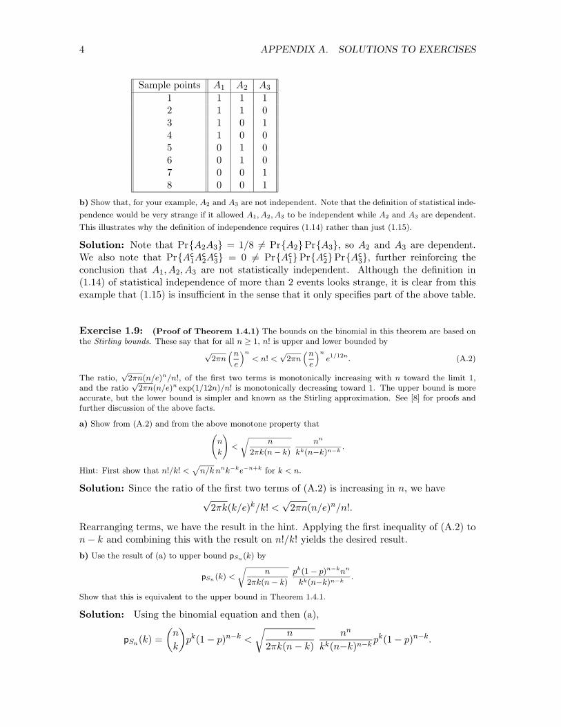
4 APPENDIX A. SOLUTIONS TO EXERCISES
Sample points A1 A2 A3
1 1 1 12 1 1 03 1 0 14 1 0 05 0 1 06 0 1 07 0 0 18 0 0 1
b) Show that, for your example, A2 and A3 are not independent. Note that the definition of statistical inde-
pendence would be very strange if it allowed A1, A2, A3 to be independent while A2 and A3 are dependent.
This illustrates why the definition of independence requires (1.14) rather than just (1.15).
Solution: Note that Pr{A2A3} = 1/8 6= Pr{A2}Pr{A3}, so A2 and A3 are dependent.We also note that Pr{Ac
1Ac2A
c3} = 0 6= Pr{Ac
1}Pr{Ac2}Pr{Ac
3}, further reinforcing theconclusion that A1, A2, A3 are not statistically independent. Although the definition in(1.14) of statistical independence of more than 2 events looks strange, it is clear from thisexample that (1.15) is insu�cient in the sense that it only specifies part of the above table.
Exercise 1.9: (Proof of Theorem 1.4.1) The bounds on the binomial in this theorem are based onthe Stirling bounds. These say that for all n � 1, n! is upper and lower bounded by
p2⇡n
⇣ne
⌘n< n! <
p2⇡n
⇣ne
⌘ne1/12n. (A.2)
The ratio,p
2⇡n(n/e)n/n!, of the first two terms is monotonically increasing with n toward the limit 1,and the ratio
p2⇡n(n/e)n exp(1/12n)/n! is monotonically decreasing toward 1. The upper bound is more
accurate, but the lower bound is simpler and known as the Stirling approximation. See [8] for proofs andfurther discussion of the above facts.
a) Show from (A.2) and from the above monotone property that nk
!<r
n2⇡k(n� k)
nn
kk(n�k)n�k.
Hint: First show that n!/k! <p
n/k nnk�ke�n+k for k < n.
Solution: Since the ratio of the first two terms of (A.2) is increasing in n, we havep
2⇡k(k/e)k/k! <p
2⇡n(n/e)n/n!.
Rearranging terms, we have the result in the hint. Applying the first inequality of (A.2) ton� k and combining this with the result on n!/k! yields the desired result.b) Use the result of (a) to upper bound pSn(k) by
pSn(k) <r
n2⇡k(n� k)
pk(1� p)n�knn
kk(n�k)n�k.
Show that this is equivalent to the upper bound in Theorem 1.4.1.
Solution: Using the binomial equation and then (a),
pSn(k) =✓
n
k
◆pk(1� p)n�k <
rn
2⇡k(n� k)nn
kk(n�k)n�kpk(1� p)n�k.

A.1. SOLUTIONS FOR CHAPTER 1 5
This is the the desired bound on pSn(k). Letting p = k/n, this becomes
pSn(pn) <
s1
2⇡np(1� p)ppn(1� p)n(1�p)
ppn(1� p)n(1�p)
=
s1
2⇡np(1� p)exp
✓n
p ln
p
p+ p ln
1� p
1� p
�◆,
which is the same as the upper bound in Theorem 1.4.1.
c) Show that
nk
!>r
n2⇡k(n� k)
nn
kk(n�k)n�k
1� n
12k(n� k)
�.
Solution: Use the factorial lower bound on n! and the upper bound on k and (n � k)!.This yields
✓n
k
◆>
rn
2⇡k(n� k)nn
kk(n�k)n�kexp
✓� 1
12k� 1
12(n� k)
◆
>
rn
2⇡k(n� k)nn
kk(n�k)n�k
1� n
12k(n� k)
�,
where the latter equation comes from combining the two terms in the exponent and thenusing the bound e�x > 1� x.
d) Derive the lower bound in Theorem 1.4.1.
Solution: This follows by substituting pn for k in the solution to c) and substituting thisin the binomial formula.
e) Show that �(p, p) = p ln( pp ) + (1� p) ln( 1�p
1�p ) is 0 at p = p and nonnegative elsewhere.
Solution: It is obvious that �(p, p) = 0 for p = p. Taking the first two derivatives of �(p, p)with respect to p,
@�(p, p)@p
= � ln✓
p(1� p)p(1� p)
◆@f2(p, p)
@p2=
1p(1� p)
.
Since the second derivative is positive for 0 < p < 1, the minimum of �(p, p) with respect top is 0, is achieved where the first derivative is 0, i.e., at p = p. Thus �(p, p) > 0 for p 6= p.Furthermore, �(p, p) increases as p moves in either direction away from p.
Exercise 1.11: a) For any given rv Y , express E [|Y |] in terms ofR
y<0FY (y) dy and
Ry�0
FcY
(y) dy. Hint:
Review the argument in Figure 1.4.
Solution: We have seen in (1.34) that
E [Y ] = �Z
y<0FY (y) dy +
Zy�0
FcY(y) dy.

6 APPENDIX A. SOLUTIONS TO EXERCISES
Since all negative values of Y become positive in |Y |,
E [|Y |] = +Z
y<0FY (y) dy +
Zy�0
FcY(y) dy.
To spell this out in greater detail, let Y = Y + + Y � where Y + = max{0, Y } and Y � =min{Y, 0}. Then Y = Y + + Y � and |Y | = Y + � Y � = Y + + |Y �|. Since E [Y +] =Ry�0 Fc
Y(y) dy and E [Y �] = �
Ry<0 FY (y) dy, the above results follow.
b) For some given rv X with E [|X|] < 1, let Y = X � ↵. Using (a), show that
E [|X � ↵|] =
Z ↵
�1FX(x) dx +
Z 1
↵
FcX(x) dx.
Solution: This follows by changing the variable of integration in (a). That is,
E [|X � ↵|] = E [|Y |] = +Z
y<0FY (y) dy +
Zy�0
FcY(y) dy
=Z ↵
�1FX(x) dx +
Z 1
↵Fc
X(x) dx,
where in the last step, we have changed the variable of integration from y to x� ↵.
c) Show that E [|X � ↵|] is minimized over ↵ by choosing ↵ to be a median of X. Hint: Both the easy way
and the most instructive way to do this is to use a graphical argument illustrating the above two integrals
Be careful to show that when the median is an interval, all points in this interval achieve the minimum.
Solution: As illustrated in the picture, we are minimizing an integral for which the inte-grand changes from FX(x) to Fc
X(x) at x = ↵. If FX(x) is strictly increasing in x, thenFc
X = 1� FX is strictly decreasing. We then minimize the integrand over all x by choosing↵ to be the point where the curves cross, i.e., where FX(x) = .5. Since the integrand hasbeen minimized at each point, the integral must also be minimized.
0.5
1
0
FX(x)
FcX(x)
↵
If FX is continuous but not strictly increasing, then there might be an interval over whichFX(x) = .5; all points on this interval are medians and also minimize the integral; Exercise1.10 (c) gives an example where FX(x) = 0.5 over the interval [1, 2). Finally, if FX(↵) � 0.5and FX(↵ � ✏) < 0.5 for some ↵ and all ✏ > 0 (as in parts (a) and (b) of Exercise 1.10),then the integral is minimized at that ↵ and that ↵ is also the median.
Exercise 1.12: Let X be a rv with CDF FX(x). Find the CDF of the following rv’s.
a) The maximum of n IID rv’s, each with CDF FX(x).
Solution: Let M+ be the maximum of the n rv’s X1, . . . ,Xn. Note that for any real x,M+ is less than or equal to x if and only if Xj x for each j, 1 j n. Thus
Pr{M+ x} = Pr{X1 x,X2 x, . . . ,Xn x} =nY
j=1
Pr{Xj x} ,

A.1. SOLUTIONS FOR CHAPTER 1 7
where we have used the independence of the Xj ’s. Finally, since Pr{Xj x} = FX(x) foreach j, we have FM+(x) = Pr{M+ x} =
�FX(x)
�n.
b) The minimum of n IID rv’s, each with CDF FX(x).
Solution: Let M� be the minimum of X1, . . . ,Xn. Then, in the same way as in ((a),M� > y if and only if Xj > y for 1 j n and for all choice of y. We could make thesame statement using greater than or equal in place of strictly greater than, but the strictinequality is what is needed for the CDF. Thus,
Pr{M� > y} = Pr{X1 > y,X2 > y, . . . ,Xn > y} =nY
j=1
Pr{Xj > y} ,
It follows that 1� FM�(y) =⇣1� FX(y)
⌘n.
c) The di↵erence of the rv’s defined in a) and b); assume X has a density fX(x).
Solution: There are many di�cult ways to do this, but also a simple way, based on firstconditioning on the event that X1 = x. Then X1 = M+ if and only if Xj x for 2 j n.Also, given X1 = M+ = x, we have R = M+ � M� r if and only if Xj > x � r for2 j n. Thus, since the Xj are IID,
Pr{M+=X1, R r | X1 = x} =nY
j=2
Pr{x�r < Xj x}
= [Pr{x�r < X x}]n�1 = [FX(x)� FX(x� r)]n�1 .
We can now remove the conditioning by averaging over X1 = x. Assuming that X has thedensity fX(x),
Pr{X1 = M+, R r} =Z 1
�1fX(x) [FX(x)� FX(x� r)]n�1 dx.
Finally, we note that the probability that two of the Xj are the same is 0 so the eventsXj = M+ are disjoint except with zero probability. Also we could condition on Xj = xinstead of X1 with the same argument (i.e., by using symmetry), so Pr{Xj = M+, R r} =Pr{X1 = M+ R r} It follows that
Pr{R r} =Z 1
�1nfX(x) [FX(x)� FX(x� r)]n�1 dx.
The only place we really needed the assumption that X has a PDF was in asserting thatthe probability that two or more of the Xj ’s are jointly equal to the maximum is 0. Theformula can be extended to arbitrary CDF’s by being careful about this possibility.
These expressions have a simple form if X is exponential with the PDF �e��x for x � 0.Then
Pr{M� � y} = e�n�y; Pr{M+ y} =�1� e��y
�n; Pr{R y} =�1� e��y
�n�1.
We will see how to derive the above expression for Pr{R y} in Chapter 2.

8 APPENDIX A. SOLUTIONS TO EXERCISES
Exercise 1.13: Let X and Y be rv’s in some sample space ⌦ and let Z = X + Y , i.e., for each! 2 ⌦, Z(!) = X(!) + Y (!). The purpose of this exercise is to show that Z is a rv. This is a mathematicalfine point that many readers may prefer to simply accept without proof.
a) Show that the set of ! for which Z(!) is infinite or undefined has probability 0.
Solution: Note that Z can be infinite (either ±1) or undefined only when either X orY are infinite or undefined. Since these are events of zero probability, Z can be infinite orundefined only with probability 0.
b) We must show that {! 2 ⌦ : Z(!) ↵} is an event for each real ↵, and we start by approximating
that event. To show that Z = X + Y is a rv, we must show that for each real number ↵, the set {! 2 ⌦ :
X(!) + Y (!) ↵} is an event. Let B(n, k) = {! : X(!) k/n}T{Y (!) ↵ + (1�k)/n} for integer k > 0.
Let D(n) =S
k B(n, k), and show that D(n) is an event.
Solution: We are trying to show that {Z ↵} is an event for arbitrary ↵ and doing thisby first quantizing X and Y into intervals of size 1/n where k is used to number thesequantized elements. Part (c) will make sense of how this is related to {Z ↵, but fornow we simply treat the sets as defined. Each set B(n, k) is an intersection of two events,namely the event {! : X(!) k/n} and the event {! : Y (!) ↵ + (1�k)/n}; these mustbe events since X and Y are rv’s. For each n, D(n) is a countable union (over k) of thesets B(n, k), and thus D(n) is an event for each n and each ↵
c) On a 2 dimensional sketch for a given ↵, show the values of X(!) and Y (!) for which ! 2 D(n). Hint:
This set of values should be bounded by a staircase function.
Solution:
x
y
@@@@@@@
@@@@
� 1n 0
1n
2n
3n
↵
↵�1/n
↵�2/n
↵
The region D(n) is sketched for ↵n = 5; it is the region below the staircase function above.The kth step of the staircase, extended horizontally to the left and vertically down is theset B(n, k). Thus we see that D(n) is an upper bound to the set {Z ↵}, which is thestraight line of slope -1 below the staircase.
d) Show that
{! : X(!) + Y (!) ↵} =\
n�1D(n). (A.3)
Explain why this shows that Z = X + Y is a rv.
Solution: The region {! : X(!) + Y (!) ↵} is the region below the diagonal line ofslope -1 that passes through the point (0,↵). This region is thus contained in D(n) foreach n � 1 and is thus contained in
Tn�1 D(n). On the other hand, each point ! for which
X(!)+Y (!) > ↵ is not contained in D(n) for su�ciently large n. This verifies (A.3). Since

A.1. SOLUTIONS FOR CHAPTER 1 9
D(n) is an event, the countable intersection is also an event, so {! : X(!) + Y (!) ↵} isan event. This applies for all ↵. This, in conjunction with (a), shows that Z is a rv.
e) Explain why this implies that if X1, X2, . . . , Xn are rv’s, then Y = X1 + X2 + · · · + Xn is a rv. Hint:
Only one or two lines of explanation are needed.
Solution: We have shown that X1 + X2 is a rv, so (X1 + X2) + X3 is a rv, etc.
Exercise 1.15: (Stieltjes integration) a) Let h(x) = u(x) and FX(x) = u(x) where u(x) is the unit
step, i.e., u(x) = 0 for �1 < x < 0 and u(x) = 1 for x � 0. Using the definition of the Stieltjes integral
in Footnote 19, show thatR 1
�1h(x)dFX(x) does not exist. Hint: Look at the term in the Riemann sum
including x = 0 and look at the range of choices for h(x) in that interval. Intuitively, it might help initially
to view dFX(x) as a unit impulse at x = 0.
Solution: The Riemann sum for this Stieltjes integral isP
n h(xn)[F(yn)� F(yn�1)] whereyn�1 < xn yn. For any partition {yn; n � 1}, consider the k such that yk�1 < 0 yk andconsider choosing either xn < 0 or xn � 0. In the first case h(xn)[F(yn)� F(yn�1)] = 0 andin the second h(xn)[F(yn) � F(yn�1)] = 1. All other terms are 0 and this can be done forall partitions as � ! 0, so the integral is undefined.
b) Let h(x) = u(x � a) and FX(x) = u(x � b) where a and b are in (�1, +1). Show thatR 1
�1h(x)dFX(x)
exists if and only if a 6= b. Show that the integral has the value 1 for a < b and the value 0 for a > b. Argue
that this result is still valid in the limit of integration over (�1, 1).
Solution: Using the same argument as in (a) for any given partition {yn; n � 1}, considerthe k such that yk�1 < b yk. If a = b, xk can be chosen to make h(xk) either 0 or 1,causing the integral to be undefined as in (a). If a < b, then for a su�ciently fine partion,h(xk) = 1 for all xk such that yk�1 < xk yk. Thus that term in the Riemann sum is1. For all other n, FX(yn) � FX(yn�1) = 0, so the Riemann sum is 1. For a > b and kas before, h(xk) = 0 for a su�ciently fine partition, and the integral is 0. The argumentdoes not involve the finite limits of integration, so the integral remains the same for infinitelimits.
c) Let X and Y be independent discrete rv’s, each with a finite set of possible values. Show thatR1�1 FX(z�
y)dFY (y), defined as a Stieltjes integral, is equal to the distribution of Z = X + Y at each z other than the
possible sample values of Z, and is undefined at each sample value of Z. Hint: Express FX and FY as sums
of unit steps. Note: This failure of Stieltjes integration is not a serious problem; FZ(z) is a step function,
and the integral is undefined at its points of discontinuity. We automatically define FZ(z) at those step
values so that FZ is a CDF (i.e., is continuous from the right). This problem does not arise if either X or
Y is continuous.
Solution: Let X have the PMF {p(x1), . . . , p(xK)} and Y have the PMF {pY (y1), . . . , pY (yJ)}.Then FX(x) =
PKk=1 p(xk)u(x� xk) and FY (y) =
PJj=1 q(yj)u(y � yj). Then
Z 1
�1FX(z � y)dFY (y) =
KXk=1
JXj=1
Z 1
�1p(xk)q(yj)u(z � yj � xk)du(y � yj).
From (b), the integral above for a given k, j exists unless z = xk + yj . In other words, theStieltjes integral gives the CDF of X + Y except at those z equal to xk + yj for some k, j,

10 APPENDIX A. SOLUTIONS TO EXERCISES
i.e., equal to the values of Z at which FZ(z) (as found by discrete convolution) has stepdiscontinuities.
To give a more intuitive explanation, FX(x) = Pr{X x} for any discrete rv X has jumpsat the sample values of X and the value of FX(xk) at any such xk includes p(xk), i.e., FX
is continuous to the right. The Riemann sum used to define the Stieltjes integral is notsensitive enough to ‘see’ this step discontinuity at the step itself. Thus, the stipulation thatZ be continuous on the right must be used in addition to the Stieltjes integral to define FZ
at its jumps.
Exercise 1.16: Let X1, X2, . . . , Xn, . . . be a sequence of IID continuous rv’s with the common probabilitydensity function fX(x); note that Pr{X=↵} = 0 for all ↵ and that Pr{Xi=Xj} = 0 for all i 6= j. For n � 2,define Xn as a record-to-date of the sequence if Xn > Xi for all i < n.
a) Find the probability that X2 is a record-to-date. Use symmetry to obtain a numerical answer without
computation. A one or two line explanation should be adequate).
Solution: X2 is a record-to-date with probability 1/2. The reason is that X1 and X2 areIID, so either one is larger with probability 1/2; this uses the fact that they are equal withprobability 0 since they have a density.
b) Find the probability that Xn is a record-to-date, as a function of n � 1. Again use symmetry.
Solution: By the same symmetry argument, each Xi, 1 i n is equally likely to be thelargest, so that each is largest with probability 1/n. Since Xn is a record-to-date if andonly if it is the largest of X1, . . . ,Xn, it is a record-to-date with probability 1/n.
c) Find a simple expression for the expected number of records-to-date that occur over the first m trials for
any given integer m. Hint: Use indicator functions. Show that this expected number is infinite in the limit
m !1.
Solution: Let In be 1 if Xn is a record-to-date and be 0 otherwise. Thus E [Ii] is theexpected value of the ‘number’ of records-to-date (either 1 or 0) on trial i. That is
E [In] = Pr{In = 1} = Pr{Xn is a record-to-date} = 1/n.
Thus
E [records-to-date up to m] =mX
n=1
E [In] =mX
n=1
1n
.
This is the harmonic series, which goes to 1 in the limit m ! 1. If you are unfamiliarwith this, note that
P1n=1 1/n �
R11
1x dx = 1.
Exercise 1.23: a) Suppose X, Y and Z are binary rv’s, each taking on the value 0 with probability 1/2
and the value 1 with probability 1/2. Find a simple example in which X, Y , Z are statistically dependent
but are pairwise statistically independent (i.e., X, Y are statistically independent, X, Z are statistically
independent, and Y , Z are statistically independent). Give pXY Z(x, y, z) for your example. Hint: In the
simplest example, there are four joint values for x, y, z that have probability 1/4 each.
Solution: The simplest solution is also a very common relationship between 3 bnary rv’s.The relationship is that X and Y are IID and Z = X �Y where � is modulo two addition,

A.1. SOLUTIONS FOR CHAPTER 1 11
i.e., addition with the table 0� 0 = 1� 1 = 0 and 0� 1 = 1� 0 = 1. Since Z is a functionof X and Y , there are only 4 sample values, each of probability 1/4. The 4 possible samplevalues for (XY Z) are then (000), (011), (101) and (110). It is seen from this that all pairsof X,Y,Z are statistically independentb) Is pairwise statistical independence enough to ensure that
EhYn
i=1Xi
i=Yn
i=1E [Xi] .
for a set of rv’s X1, . . . , Xn?
Solution: No, (a) gives an example, i.e., E [XY Z] = 0 and E [X]E [Y ]E [Z] = 1/8.
Exercise 1.25: For each of the following random variables, find the endpoints r� and r+ of the intervalfor which the moment generating function g(r) exists. Determine in each case whether g(r) exists at r� andr+. For parts a) and b) you should also find and sketch g(r). For parts c) and d), g(r) has no closed form.
a) Let �, ✓, be positive numbers and let X have the density.
fX(x) =12� exp(��x); x � 0; fX(x) =
12✓ exp(✓x); x < 0.
Solution: Integrating to find gX(r) as a function of � and ✓, we get
gX(r) =Z 0
�1
12✓e✓x+rx dx +
Z 1
0
12�e��x+rx dx =
✓
2(✓ + r)+
�
2(�� r)
The first integral above converges for r > �✓ and the second for r < �. Thus r� = �✓ andr+ = �. The MGF does not exist at either end point.
b) Let Y be a Gaussian random variable with mean m and variance �2.
Solution: Calculating the MGF by completing the square in the exponent,
gY (r) =Z 1
�1
1p2⇡�2
exp✓�(y �m)2
2�2+ ry
◆dy
=Z 1
�1
1p2⇡�2
exp✓�(y �m� r�2)2
2�2+ rm +
r2�2
2
◆dy
= exp✓
rm +r2�2
2
◆,
where the final equality arises from realizing that the other terms in the equation aboverepresent a Gaussian density and thus have unit integral. Note that this is the same as theresult in Table 1.1. This MGF is finite for all finite r so r� = �1 and r+ = 1. Also gY (r)is infinite at each endpoint.c) Let Z be a nonnegative random variable with density
fZ(z) = k(1 + z)�2 exp(��z); z � 0.
where � > 0 and k = [R
z�0(1+z)�2 exp(��z)dz]�1. Hint: Do not try to evaluate gZ(r). Instead, investigate
values of r for which the integral is finite and infinite.
Solution: Writing out the formula for gZ(r), we have
gZ(r) =Z 1
0k(1 + z)�2 exp
�(r � �)z
�dz.

12 APPENDIX A. SOLUTIONS TO EXERCISES
This integral is clearly infinite for r > � and clearly finite for r < �. For r = �, theexponential term disappears, and we note that (1 + z)�2 is bounded for z 1 and goes to0 as z�2 as z ! 1, so the integral is finite. Thus r+ belongs to the region where gZ(r) isfinite.
The whole point of this is that the random variables for which r+ = � are those for whichthe density or PMF go to 0 with increasing z as e��z. Whether or not gZ(�) is finitedepends on the coe�cient of e��z.
d) For the Z of (c), find the limit of �0(r) as r approaches � from below. Then replace (1+ z)2 with |1+ z|3
in the definition of fZ(z) and K and show whether the above limit is then finite or not. Hint: no integration
is required.
Solution: Di↵erentiating gZ(r) with respect to r,
g0Z(r) =Z 1
0kz(1 + z)�2 exp
�(r � �)z
�dz.
For r = �, the above integrand approaches 0 as 1/z and thus the integral does not converge.In other words, although gZ(�) is finite, the slope of gZ(r) is unbounded as r ! � frombelow. If (1 + z)�2 is repaced with (1 + z)�3 (with k modified to maintain a probabilitydensity), we see that as z ! 1, z(1 + z)�3 goes to 0 as 1/z2, so the integral converges.Thus in this case the slope of gZ(r) remains bounded for r < �.
Exercise 1.26: a) Assume that the random variable X has a moment generating function gX(r) that is
finite in the interval (r�, r+), r� < 0 < r+, and assume r� < r < r+ throughout. For any finite constant c,
express the moment generating function of X�c, i.e., g(X�c)(r) in terms of the moment generating function
of X. Show that g00(X�c)(r) � 0.
Solution: Note that g(X�c)(r) = E [exp(r(X � c))] = gX(r)e�cr. Thus r+ and r� are thesame for X and X � c. Thus (see Footnote 24), the derivatives of g(X�c)(r) with respect tor are finite. The first two derivatives are then given by
g0(X�c)(r) = E [(X � c) exp(r(X � c))] ,
g00(X�c)(r) = E⇥(X � c)2 exp(r(X � c))
⇤� 0,
since (X � c)2 exp(r(X � c)) � 0 for all x.
b) Show that g00(X�c)(r) = [g00X(r)� 2cg0X(r) + c2gX(r)]e�rc.
Solution: Writing (X � c)2 as X2 � 2cX + c2, we get
g00(X�c)(r) = E⇥X2 exp(r(X � c))
⇤� 2cE [X exp(r(X � c))] + c2E [exp(r(X � c))]
=⇥E⇥X2 exp(rX)
⇤� 2cE [X exp(rX)] + c2E [exp(rX)]
⇤exp(�rc)
=⇥g00X(r)� 2cg0X(r) + c2g(r)
⇤exp(�rc).
c) Use a) and b) to show that g00X(r)gX(r)� [g0X(r)]2 � 0, and that �00X(r) � 0. Hint: Let c = g0X(r)/gX(r).

A.1. SOLUTIONS FOR CHAPTER 1 13
Solution: With the suggested choice for c,
g00(X�c)(r) =g00X(r)� 2
(g0X(r))2
gX(r)+
(g0X(r))2
gX(r)
�exp(�rc)
=gX(r)g00X(r)� [g0X(r)]2
gX(r)
�exp(�cr).
Since this is nonnegative from (a), we see that
�00X(r) = gX(r)g00X(r)� [g0X(r)]2 � 0.
d) Assume that X is non-atomic, i.e., that there is no value of c such that Pr{X = c} = 1. Show that the
inequality sign “ � “ may be replaced by “ > “ everywhere in a), b) and c).
Solution: Since X is non-atomic, (X � c) must be non-zero with positive probability, andthus from (a), g00(X�c)(r) > 0. Thus the inequalities in parts b) and c) are strict also.
Exercise 1.28: Suppose the rv X is continuous and has the CDF FX(x). Consider another rv
Y = FX(X). That is, for each sample point ! such that X(!) = x, we have Y (!) = FX(x). Show that Y is
uniformly distributed in the interval 0 to 1.
Solution: For simplicity, first assume that FX(x) is strictly increasing in x, thus havingthe following appearance:
x
FX(x)
F�1X (y)
yIf FX(x) = y, then F�1
X (y) = x
Since FX(x) is continuous in x and strictly increasing from 0 to 1, there must be an inversefunction F�1
X such that for each y 2 (0, 1), F�1X (y) = x for that x such that FX(x) = y.
For this y, then, the event {FX(X) y} is the same as the event {X F�1X (y)}. This is
illustrated in the figure above. Using this equality for the given y,
Pr{Y y} = Pr{FX(X) y} = Pr�X F�1
X (y)
= FX(F�1X (y)) = y.
where in the final equation, we have used the fact that F�1X is the inverse function of FX .
This relation, for all y 2 (0, 1), shows that Y is uniformly distributed between 0 and 1.
If FX is not strictly increasing, i.e., if there is any interval over which FX(x) has a constantvalue y, then we can define F�1
X (y) to have any given value within that interval. The aboveargument then still holds, although F�1
X is no longer the inverse of FX .
If there is any discrete point, say z at which Pr{X = z} > 0, then FX(x) cannot take onvalues in the open interval between FX(z)� a and FX(z) where a = Pr{X = z}. Thus FX
is uniformly distributed only for continuous rv’s.

14 APPENDIX A. SOLUTIONS TO EXERCISES
Exercise 1.34: We stressed the importance of the mean of a rv X in terms of its association with thesample average via the WLLN. Here we show that there is a form of WLLN for the median and for theentire CDF, say FX(x) of X via su�ciently many independent sample values of X.
a) For any given x, let Ij(x) be the indicator function of the event {Xj x} where X1, X2, . . . , Xj , . . . are
IID rv’s with the CDF FX(x). State the WLLN for the IID rv’s {I1(x), I2(x), . . . }.
Solution: The mean value of Ij(x) is FX(x) and the variance (after a short calculation) isFX(x)Fc
X(x). This is finite (and in fact at most 1/4), so Theorem 1.7.1 applies and
limn!1
Pr
8<:��� 1n
nXj=1
Ij(x)� FX(x)��� > ✏
9=; = 0 for all x and ✏ > 0. (A.4)
This says that if we take n samples of X and use (1/n)Pn
j=1 Ij(x) to approximate the CDFFX(x) at each x, then the probability that the approximation error exceeds ✏ at any givenx approaches 0 with increasing n.
b) Does the answer to (a) require X to have a mean or variance?
Solution: No. As pointed out in a), Ij(x) has a mean and variance whether or not X does,so Theorem 1.7.1 applies.c) Suggest a procedure for evaluating the median of X from the sample values of X1, X2, . . . . Assume thatX is a continuous rv and that its PDF is positive in an open interval around the median. You need not beprecise, but try to think the issue through carefully.
What you have seen here, without stating it precisely or proving it is that the median has a law of large
numbers associated with it, saying that the sample median of n IID samples of a rv is close to the true
median with high probability.
Solution: Note that (1/n)Pn
j=1 Ij(y) is a rv for each y. Any sample function x1, . . . , xn
of X1, . . . ,Xn maps into a sample value of (1/n)Pn
j=1 Ij(y) for each y. We can view thiscollection of sample values as a function of y. Any such sample function is non-decreasingin y, and as seen in (a) is an approximation to FX(y) at each y. This function of y has allthe characteristics of a CDF itself, so we can let ↵n be the median of (1/n)
Pnj=1 Ij(y) as
a function of y. Let ↵ be the true median of X and let � > 0 be arbitrary. Note that if(1/n)
Pnj=1 Ij(↵ � �) < .5, then ↵n > ↵ � �. Similarly, if (1/n)
Pnj=1 Ij(↵ + �) > .5, then
↵n < ↵ + �. Thus,
Pr���↵n � ↵
�� � � Pr
8<:
1n
nXj=1
Ij(↵� �) � .5
9=;+ Pr
8<:
1n
nXj=1
Ij(↵ + �) .5
9=; .
Because of the assumption of a nonzero density, there is some ✏1 > 0 such that FX(a� �) <.5� ✏1 and some ✏2 > 0 such that FX(a� �) > .5 + ✏1. Thus,
Pr���↵n � ↵
�� � �
Pr
8<:��� 1n
nXj=1
Ij(↵� �)� FX(↵� �)��� > ✏1
9=;
+ Pr
8<:��� 1n
nXj=1
Ij(↵ + �)� FX(↵ + �)��� > ✏2
9=; .

A.1. SOLUTIONS FOR CHAPTER 1 15
From (A.4), the limit of this as n !1 is 0, which is a WLLN for the median. With a greatdeal more fussing, the same result holds true without the assumption of a positive densityif we allow ↵ above to be any median in cases where the median is nonunique.
Exercise 1.35 a) Show that for any integers 0 < k < n, n
k + 1
!
nk
!n� k
k.
Solution: ✓n
k + 1
◆=
n!(k + 1)!(n� k � 1)!
=n!
k!(k + 1)(n� k)!/(n� k)
=✓
n
k
◆n� k
k + 1✓
n
k
◆n� k
k. (A.5)
b) Extend (a) to show that, for all ` n� k, n
k + `
!
nk
!n� k
k
�`
. (A.6)
Solution: Using k + ` in place of k + 1 in (A.5),✓n
k + `
◆✓
n
k + `� 1
◆n� k � (`� 1)
k + `� 1
�✓
n
k + `� 1
◆n� k
k
�.
Applying recursion on `, we get (A.6).c) Let p = k/n and q = 1� p. Let Sn be the sum of n binary IID rv’s with pX(0) = q and pX(1) = p. Showthat for all ` n� k,
pSn(k + `) pSn(k)
✓qppq
◆`
. (A.7)
Solution: Using (b),
pSn(k + `) =✓
n
k + `
◆pk+`qn�k�`
✓n
k
◆n� k
k
�` p
q
�`
pkqn�k = pSn(k)qp
pq
�`
.
d) For k/n > p, show that Pr{Sn � k} pqp�p pSn(k).
Solution: Using the bound in (A.7), we get
Pr{Sn � k} =n�kX`=0
pSn(k+`) n�kX`=0
pSn(k)✓
qp
pq
◆`
pSn(k)1
1� qp/pq= pSn(k)
pq
pq � qp(A.8)
= pSn(k)pq
p(1� p)� (1� p)p= pSn(k)
pq
p� p.
e) Now let ` be fixed and k = dnpe for fixed p such that 1 > p > p. Argue that as n !1,
pSn(k + `) ⇠ pSn(k)
✓qppq
◆`
and Pr{Sn � k} ⇠ pqp� p
pSn(k),
16 APPENDIX A. SOLUTIONS TO EXERCISES
where a(n) ⇠ b(n) means that limn!1 a(n)/b(n) = 1.
Solution: Note that (A.6) provides an upper bound to� nk+`
�and a slight modification of
the same argument provides the lower bound� nk+`
���nk
��n�k�`
k+`
�`. Taking the ratio of theupper to lower bound for fixed ` and p as n !1, we see that
✓n
k + `
◆⇠
✓n
k
◆n� k
k
�`
so that
pSn(k + `) ⇠ pSn(k)(qp/pq)` (A.9)
follows. Replacing the upper bound in (A.8) with the asymptotic equality in (A.9), andletting ` grow very slowly with n, we get Pr{Sn � k} ⇠ pq
p�p pSn(k).
Exercise 1.39: Let {Xi; i � 1} be IID binary rv’s. Let Pr{Xi = 1} = �, Pr{Xi = 0} = 1 � �. LetSn = X1 + · · · + Xn. Let m be an arbitrary but fixed positive integer. Think! then evaluate the followingand explain your answers:
a) limn!1P
i: n��min�+m Pr{Sn = i}.
Solution: It is easier to reason about the problem if we restate the sum in the followingway:
Xi: n��min�+m
Pr{Sn = i} = Pr{n� �m Sn n� + m}
= Pr��m Sn � nX m
= Pr
⇢�m
�p
n Sn � nX
�p
n m
�p
n
�,
where � is the standard deviation of X. Now in the limit n ! 1, (Sn � nX)/�p
napproaches a normalized Gaussian rv in distribution, i.e.,
limn!1
Pr⇢�m
�p
n Sn � nX
�p
n m
�p
n
�= lim
n!1
⇥�� m
�p
n
�� �
� �m
�p
n
�⇤= 0.
This can also be seen immediately from the binomial distribution as it approaches a discreteGaussian distribution. We are looking only at essentially the central 2m terms of thebinomial, and each of those terms goes to 0 as 1/
pn with increasing n.
b) limn!1P
i :0in�+m Pr{Sn = i}.
Solution: Here all terms on lower side of the distribution are included and the upper sideis bounded as in (a). Arguing in the same way as in (a), we see that
Xi:0in�+m
Pr{Sn = i} = Pr⇢
Sn � nX
�p
n m
�p
n
�.
In the limit, this is �(0) = 1/2.
c) limn!1P
i :n(��1/m)in(�+1/m) Pr{Sn = i}.

A.1. SOLUTIONS FOR CHAPTER 1 17
Solution: Here the number of terms included in the sum is increasing linearly with n, andthe appropriate mechanism is the WLLN.
Xi:n(��1/m)in(�+1/m)
Pr{Sn = i} = Pr⇢� 1
m Sn � nX
n 1
m
�.
In the limit n !1, this is 1 by the WLLN. The essence of this exercise has been to scalethe random variables properly to go the limit. We have used the CLT and the WLLN, butone could guess the answers immediately by recognizing what part of the distribution isbeing looked at.
Exercise 1.44: Let X1, X2 . . . be a sequence of IID rv’s each with mean 0 and variance �2. Let
Sn = X1 + · · · + Xn for all n and consider the random variable Sn/�p
n � S2n/�p
2n. Find the limiting
CDF for this sequence of rv’s as n ! 1. The point of this exercise is to see clearly that the CDF of
Sn/�p
n � S2n/�p
2n is converging in n but that the sequence of rv’s is not converging in any reasonable
sense.
Solution: If we write out the above expression in terms of the Xi, we get
Sn
�p
n� S2n
�p
2n=
nXi=1
Xi
1
�p
n� 1
�p
2n
��
2nXi=n+1
Xi
�p
2n.
The first sum above approaches a Gaussian distribution of variance (1 � 1/p
2)2 and thesecond sum approaches a Gaussian distribution of variance 1/2. Since these two terms areindependent, the di↵erence approaches a Gaussian distribution of variance 1+(1�1/
p2)2.
This means that the distribution of the di↵erence does converge to this Gaussian rv asn !1. As n increases, however, this di↵erence slowly changes, and each time n is doubled,the new di↵erence is only weakly correlated with the old di↵erence.
Note that Sn/n�X behaves in this same way. The CDF converges as n !1, but the rv’sthemselves do not approach each other in any reasonable way. The point of the problemwas to emphasize this property.
Exercise 1.47: Consider a discrete rv X with the PMF
pX(�1) = (1� 10�10)/2,
pX(1) = (1� 10�10)/2,
pX(1012) = 10�10.
a) Find the mean and variance of X. Assuming that {Xm; m � 1} is an IID sequence with the distribution
of X and that Sn = X1 + · · ·+ Xn for each n, find the mean and variance of Sn. (no explanations needed.)
Solution: X = 100 and �2X = 1014 + (1 � 10�10) � 104 ⇡ 1014. Thus Sn = 100n and
�2Sn⇡ n⇥ 1014.
b) Let n = 106 and describe the event {Sn 106} in words. Find an exact expression for Pr�Sn 106
=
FSn(106).
Solution: This is the event that all 106 trials result in ±1. That is, there are no occurrencesof 1012. Thus Pr
�Sn 106
= (1� 10�10)106

18 APPENDIX A. SOLUTIONS TO EXERCISES
c) Find a way to use the union bound to get a simple upper bound and approximation of 1� FSn(106).
Solution: From the union bound, the probability of one or more occurrences of the samplevalue 1012 out of 106 trials is bounded by a sum of 106 terms, each equal to 10�10, i.e.,1� FSn(106) 10�4. This is also a good approximation, since we can write
(1� 10�10)106
= exp⇣106 ln(1� 10�10)
⌘⇡ exp(106 · 10�10) ⇡ 1� 10�4.
d) Sketch the CDF of Sn for n = 106. You can choose the horizontal axis for your sketch to go from �1
to +1 or from �3 ⇥ 103 to 3 ⇥ 103 or from �106 to 106 or from 0 to 1012, whichever you think will best
describe this CDF.
Solution: Conditional on no occurrences of 1012, Sn simply has a binomial distribution.We know from the central limit theorem for the binomial case that Sn will be approxi-mately Gaussian with mean 0 and standard deviation 103. Since one or more occurrencesof 1012 occur only with probability 10�4, this can be neglected in the sketch, so the CDF isapproximately Gaussian with 3 sigma points at ±3⇥ 103. There is a little blip, in the 4thdecimal place out at 1012 which doesn’t show up well in the sketch, but of course could beimportant for some purposes such as calculating �2.
103 3⇥ 103
1
00
FSn
e) Now let n = 1010. Give an exact expression for Pr�Sn 1010
and show that this can be approximated
by e�1. Sketch the CDF of Sn for n = 1010, using a horizontal axis going from slightly below 0 to slightly
more than 2⇥ 1012. Hint: First view Sn as conditioned on an appropriate rv.
Solution: First consider the PMF pB(j) of the number B = j of occurrences of the value1012. We have
pB(j) =✓
1010
j
◆pj(1� p)10
10�j where p = 10�10
pB(0) = (1� p)1010= exp{1010 ln[1� p]} ⇡ exp(�1010p) = e�1
pB(1) = 1010p(1� p)1010�1 = (1� p)1010�1 ⇡ e�1
pB(2) =✓
1010
2
◆p2(1� p)1010�2 ⇡ 1
2e�1.
Conditional on B = j, Sn will be approximately Gaussian with mean 1012j and standarddeviation 105. Thus FSn(s) rises from 0 to e�1 over a range from about �3⇥105 to +3⇥105.It then stays virtually constant up to about 1012�3⇥105. It rises to 2/e by 1012 +3⇥105.

A.1. SOLUTIONS FOR CHAPTER 1 19
It stays virtually constant up to 2⇥ 1012� 3⇥ 105 and rises to 2.5/e by 2⇥ 1012 + 3⇥ 105.When we sketch this, it looks like a staircase function, rising from 0 to 1/e at 0, from 1/eto 2/e at 1012 and from 2/e to 2.5/e at 2⇥ 1012. There are smaller steps at larger values,but they would not show up on the sketch.
d) Can you make a qualitative statement about how the distribution function of a rv X a↵ects the required
size of n before the WLLN and the CLT provide much of an indication about Sn.
Solution: It can be seen that for this peculiar rv, Sn/n is not concentrated around itsmean even for n = 1010 and Sn/
pn does not look Gaussian even for n = 1010. For this
particular distribution, n has to be so large that B, the number of occurrences of 1012, islarge, and this requires n >> 1010. This illustrates a common weakness of limit theorems.They say what happens as a parameter (n in this case) becomes su�ciently large, but ittakes extra work to see how large that is.
Exercise 1.48: Let {Yn; n � 1} be a sequence of rv’s and assume that limn!1 E [|Yn|] = 0. Show that
{Yn; n � 1} converges to 0 in probability. Hint 1: Look for the easy way. Hint 2: The easy way uses the
Markov inequality.
Solution: Applying the Markov inequality to |Yn| for arbitrary n and arbitrary ✏ > 0, wehave
Pr{|Yn| � ✏} E [|Yn|]✏
.
Thus going to the limit n !1 for the given ✏,
limn!1
Pr{|Yn| � ✏} = 0.
Since this is true for every ✏ > 0, this satisfies the definition for convergence to 0 in proba-bility.

20 APPENDIX A. SOLUTIONS TO EXERCISES
A.2 Solutions for Chapter 2
Exercise 2.1: a) Find the Erlang density fSn(t) by convolving fX(x) = � exp(��x), x � 0 with itself n
times.
Solution: For n = 2, we convolve fX(x) with itself.
fS2(t) =Z t
0fX1(x)fX2(t� x) dx =
Z t
0�e��x�e��(t�x) dx = �2te��t.
For larger n, convolving fX(x) with itself n times is found by taking the convolution n�1times, i.e., fSn�1(t), and convolving this with fX(x). Starting with n = 3,
fS3(t) =Z t
0fS2(x)fX3(t� x) dx =
Z t
0�2xe��x�e��(t�x) dx =
�3t2
2e��t
fS4(t) =Z t
0
�3x2
2e��x · �e�(t�x) dx =
�4t3
3!e��t.
We now see the pattern; each additional integration increases the power of � and t by 1and multiplies the denominator by n � 1. Thus we hypothesize that fSn(t) = �ntn�1
n! e��t.If one merely wants to verify the well-known Erlang density, one can simply use inductionfrom the beginning, but it is more satisfying, and not that much more di�cult, to actuallyderive the Erlang density, as done above.
b) Find the moment generating function of X (or find the Laplace transform of fX(x)), and use this to find
the moment generating function (or Laplace transform) of Sn = X1 + X2 + · · · + Xn.
Solution: The formula for the MGF is almost trivial here,
gX(r) =Z 1
0�e��xerx dx =
�
�� rfor r < �.
Since Sn is the sum of n IID rv’s,
gSn(r) =⇥gX(r)
⇤n =✓
�
�� r
◆n
.
c) Find the Erlang density by starting with (2.15) and then calculating the marginal density for Sn.
Solution: To find the marginal density, fSn(sn), we start with the joint density in (2.15)and integrate over the region of space where s1 s2 · · · sn. It is a peculiar integral,since the integrand is constant and we are just finding the volume of the n� 1 dimensionalspace in s1, . . . , sn�1 with the inequality constraints above. For n = 2 and n = 3, we have
fS2(s2) = �2e��s2
Z s2
ods1 =
⇣�2e��s2
⌘s2
fS3(s3) = �3e��s3
Z s3
0
Z s2
0ds1
�ds2 = �3e��s3
Z s3
0s2 ds2 =
⇣�3e��s3
⌘ s23
2.
A.2. SOLUTIONS FOR CHAPTER 2 21
The critical part of these calculations is the calculation of the volume, and we can do thisinductively by guessing from the previous equation that the volume, given sn, of the n� 1dimensional space where 0 < s1 < · · · < sn�1 < sn is sn�1
n /(n�1)!. We can check that by
Z sn
0
Z sn�1
0· · ·Z s2
0ds1 . . . dsn�2
�dsn�1 =
Z sn
0
sn�2n�1
(n� 2)!dsn�1 =
sn�1n
(n�1)!.
This volume integral, multiplied by �ne��sn , is then the desired marginal density.
A more elegant and instructive way to calculate this volume is by first observing that thevolume of the n � 1 dimensional cube, sn on a side, is sn�1
n . Each point in this cube canbe visualized as a vector (s1, s2, . . . , sn�1). Each component lies in (0, sn), but the cubedoesn’t have the ordering constraint s1 < s2 < · · · < sn�1. By symmetry, the volume ofpoints in the cube satisfying this ordering constraint is the same as the volume in whichthe components s1, . . . sn�1 are ordered in any other particular way. There are (n � 1)!di↵erent ways to order these n� 1 components (i.e., there are (n� 1)! permutations of thecomponents), and thus the volume with the ordering constraints, is sn�1
n /(n� 1)!.
Exercise 2.3: The purpose of this exercise is to give an alternate derivation of the Poisson distributionfor N(t), the number of arrivals in a Poisson process up to time t. Let � be the rate of the process.
a) Find the conditional probability Pr{N(t) = n | Sn = ⌧} for all ⌧ t.
Solution: The condition Sn = ⌧ means that the epoch of the nth arrival is ⌧ . Conditionalon this, the event {N(t) = n} for some t > ⌧ means there have been no subsequent arrivalsfrom ⌧ to t. In other words, it means that the (n + 1)th interarrival time, Xn+1 exceedst� ⌧ . This interarrival time is independent of Sn and thus
Pr{N(t) = n | Sn = ⌧} = Pr{Xn+1 > t� ⌧} = e��(t�⌧) for t > ⌧. (A.10)
b) Using the Erlang density for Sn, use (a) to find Pr{N(t) = n}.
Solution: We find Pr{N(t) = n} simply by averaging (A.10) over Sn.
Pr{N(t)=n} =Z 1
0Pr{N(t)=n | Sn=⌧} fSn(⌧) d⌧
=Z t
0e��(t�⌧) �
n⌧n�1e��⌧
(n� 1)!d⌧
=�ne��t
(n� 1)!
Z t
0⌧n�1 d⌧ =
(�t)ne��t
n!.
Exercise 2.5: The point of this exercise is to show that the sequence of PMF’s for the counting processof a Bernoulli process does not specify the process. In other words, knowing that N(t) satisfies the binomialdistribution for all t does not mean that the process is Bernoulli. This helps us understand why thesecond definition of a Poisson process requires stationary and independent increments along with the Poissondistribution for N(t).
a) For a sequence of binary rv’s Y1, Y2, Y3, . . . , in which each rv is 0 or 1 with equal probability, find ajoint distribution for Y1, Y2, Y3 that satisfies the binomial distribution, pN(t)(k) =
�tk
�2�t for t = 1, 2, 3 and
0 k t, but for which Y1, Y2, Y3 are not independent.

22 APPENDIX A. SOLUTIONS TO EXERCISES
Your solution should contain four 3-tuples with probability 1/8 each, two 3-tuples with probability 1/4 each,
and two 3-tuples with probability 0. Note that by making the subsequent arrivals IID and equiprobable, you
have an example where N(t) is binomial for all t but the process is not Bernoulli. Hint: Use the binomial
for t = 3 to find two 3-tuples that must have probability 1/8. Combine this with the binomial for t = 2
to find two other 3-tuples with probability 1/8. Finally look at the constraints imposed by the binomial
distribution on the remaining four 3-tuples.
Solution: The 3-tuples 000 and 111 each have probability 1/8, and are the unique tuplesfor which N(3) = 0 and N(3) = 3 respectively. In the same way, N(2) = 0 only for(Y1, Y2) = (0, 0), so (0,0) has probability 1/4. Since (0, 0, 0) has probability 1/8, it followsthat (0, 0, 1) has probability 1/8. In the same way, looking at N(2) = 2, we see that (1, 1, 0)has probability 1/8.
The four remaining 3-tuples are illustrated below, with the constraints imposed by N(1)and N(2) on the left and those imposed by N(3) on the right.
⇤�1/4
1/4
1/4
1/4
0 1 00 1 11 0 01 0 1
It can be seen by inspection from the figure that if (0, 1, 0) and (1, 0, 1) each have probability1/4, then the constraints are satisfied. There is one other solution satisfying the constraints:choose (0, 1, 1) and (1, 0, 0) to each have probability 1/4.
b) Generalize (a) to the case where Y1, Y2, Y3 satisfy Pr{Yi = 1} = q and Pr{Yi = 0} = 1 � q. Assume
q < 1/2 and find a joint distribution on Y1, Y2, Y3 that satisfies the binomial distribution, but for which the
3-tuple (0, 1, 1) has zero probability.
Solution: Arguing as in (a), we see that Pr{(0, 0, 0)} = (1� q)3, Pr{(0, 0, 1)} = (1� q)2p,Pr{(1, 1, 1)} = q3, and Pr{(1, 1, 0)} = q2(1�q). The remaining four 3-tuples are constrainedas shown below.
⇤�q(1� q)
q(1� q)
2q(1� q)2
2q2(1� q)
0 1 00 1 11 0 01 0 1
If we set Pr{(0, 1, 1)} = 0, then Pr{0, 1, 0)} = q(1 � q), Pr{(1, 0, 1)} = 2q2(1 � q), andPr{(1, 0, 0)} = q(1 � q) � 2q2(1 � q) = q(1 � q)(1 � 2q). This satisfies all the binomialconstraints.
c) More generally yet, view a joint PMF on binary t-tuples as a nonnegative vector in a 2t dimensional vector
space. Each binomial probability pN(⌧)(k) =�
⌧k
�qk(1� q)⌧�k constitutes a linear constraint on this vector.
For each ⌧ , show that one of these constraints may be replaced by the constraint that the components of
the vector sum to 1.

A.2. SOLUTIONS FOR CHAPTER 2 23
Solution: There are 2t binary n-tuples and each has a probability, so the joint PMF canbe viewed as a vector of 2t numbers. The binomial probability pN(⌧)(k) =
�⌧k
�qk(1� q)⌧�k
specifies the sum of the probabilities of the n-tuples in the event {N(⌧) = k}, and thus is alinear constraint on the joint PMF. Note: Mathematically, a linear constraint specifies thata given weighted sum of components is 0. The type of constraint here, where the weightedsum is a nonzero constant, is more properly called a first-order constraint. Engineers oftenrefer to first order constraints as linear, and we follow that practice here.
SinceP⌧
k=0
�⌧k
�pkq⌧�k = 1, one of these ⌧ + 1 constraints can be replaced by the constraint
that the sum of all 2t components of the PMF is 1.
d) Using (c), show that at most (t + 1)t/2 + 1 of the binomial constraints are linearly independent. Note
that this means that the linear space of vectors satisfying these binomial constraints has dimension at least
2t � (t + 1)t/2 � 1. This linear space has dimension 1 for t = 3, explaining the results in parts a) and
b). It has a rapidly increasing dimension for t > 3, suggesting that the binomial constraints are relatively
ine↵ectual for constraining the joint PMF of a joint distribution. More work is required for the case of t > 3
because of all the inequality constraints, but it turns out that this large dimensionality remains.
Solution: We know that the sum of all the 2t components of the PMF is 1, and we saw in(c) that for each integer ⌧, 1 ⌧ t, there are ⌧ additional linear constraints on the PMFestablished by the binomial terms N(⌧ = k) for 0 k ⌧ . Since
Pt⌧=1 ⌧ = (t + 1)t/2,
we see that there are t(t + 1)/2 independent linear constraints on the joint PMF imposedby the binomial terms, in addition to the overall constraint that the components sum to1. Thus the dimensionality of the 2t vectors satisfying these linear constraints is at least2t � 1� (t + 1)t/2.
Exercise 2.9: Consider a “shrinking Bernoulli” approximation N�(m�) = Y1 + · · · + Ym to a Poissonprocess as described in Subsection 2.2.5.
a) Show that
Pr{N�(m�) = n} =
mn
!(��)n(1� ��)m�n.
Solution: This is just the binomial PMF in (1.23)b) Let t = m�, and let t be fixed for the remainder of the exercise. Explain why
lim�!0
Pr{N�(t) = n} = limm!1
mn
!✓�tm
◆n ✓1� �t
m
◆m�n
,
where the limit on the left is taken over values of � that divide t.
Solution: This is the binomial PMF in (a) with � = t/m.c) Derive the following two equalities:
limm!1
mn
!1
mn=
1n!
; and limm!1
✓1� �t
m
◆m�n
= e��t.
Solution: Note that✓
m
n
◆=
m!n!(m� n)!
=1n!
n�1Yi=0
(m� i).

24 APPENDIX A. SOLUTIONS TO EXERCISES
When this is divided by mn, each term in the product above is divided by m, so✓
m
n
◆1
mn=
1n!
n�1Yi=0
(m� i)m
=1n!
n�1Yi=0
⇣1� i
m
⌘. (A.11)
Taking the limit as m !1, each of the n terms in the product approaches 1, so the limitis 1/n!, verifying the first equality in (c). For the second,
✓1� �t
m
◆m�n
= exp(m� n) ln
⇣1� �t
m
⌘�= exp
(m� n)
⇣��t
m+ o(1/m
⌘�
= exp��t +
n�t
m+ (m� n)o(1/m)
�.
In the second equality, we expanded ln(1 � x) = �x + x2/2 · · · . In the limit m ! 1, thefinal expression is exp(��t), as was to be shown.
If one wishes to see how the limit in (A.11) is approached, we have
1n!
n�1Yi=0
⇣1� i
m
⌘=
1n!
exp
n�1Xi=1
ln⇣1� i
m
⌘!=
1n!
exp✓�n(n� 1)
2m+ o(1/m)
◆.
d) Conclude from this that for every t and every n, lim�!0 Pr{N�(t)=n} = Pr{N(t)=n} where {N(t); t > 0}is a Poisson process of rate �.
Solution: We simply substitute the results of (c) into the expression in (b), getting
lim�!0
Pr{N�(t) = n} =(�t)ne��t
n!.
This shows that the Poisson PMF is the limit of shrinking Bernoulli PMF’s, but recallfrom Exercise 2.5 that this is not quite enough to show that a Poisson process is thelimit of shrinking Bernoulli processes. It is also necessary to show that the stationaryand independent increment properties hold in the limit � ! 0. It can be seen that theBernoulli process has these properties at each increment �, and it is intuitively clear thatthese properties should hold in the limit, but it seems that carrying out all the analyticaldetails to show this precisely is neither warranted or interesting.
Exercise 2.10: Let {N(t); t > 0} be a Poisson process of rate �.
a) Find the joint probability mass function (PMF) of N(t), N(t + s) for s > 0.
Solution: Note that N(t+s) is the number of arrivals in (0, t] plus the number in�t, t+s
�.
In order to find the joint distribution of N(t) and N(t+s), it makes sense to express N(t+s)as N(t) + eN(t, t+s) and to use the independent increment property to see that eN�t, t+s)
�is independent of N(t). Thus for m > n,
pN(t)N(t+s)(n,m) = Pr{N(t)=n}Prn eN(t, t+s)=m�n)
o
=(�t)ne��t
n!⇥��s�m�n
e��s
(m� n)!,

A.2. SOLUTIONS FOR CHAPTER 2 25
where we have used the stationary increment property to see that eN(t, t+s) has the samedistribution as N(s). This solution can be rearranged in various ways, of which the mostinteresting is
pN(t)N(t+s)(n,m) =(��t+s)
�me��(s+t)
m!⇥✓
m
n
◆⇣ t
t+s
⌘n⇣ s
t+s
⌘m�n,
where the first term is pN(t+s)(m) (the probability of m arrivals in (0, t+s]) and the second,conditional on the first, is the binomial probability that n of those m arrivals occur in (0, t).
b) Find E [N(t) · N(t + s)] for s > 0.
Solution: Again expressing N(t+s) = N(t) + eN(t, t+s),
E [N(t) ·N(t+s)] = E⇥N2(t)
⇤+ E
hN(t) eN(t, t+s)
i= E
⇥N2(t)
⇤+ E [N(t)]E [N(s)]
= �t + �2t2 + �t�s.
In the final step, we have used the fact (from Table 1.2 or a simple calculation) that themean of a Poisson rv with PMF (�t)n exp(��t)/n! is �t and the variance is also �t (thusthe second moment is �t + (�t)2). This mean and variance was also derived in Exercise 2.2and can also be calculated by looking at the limit of shrinking Bernoulli processes.
c) Find Eh eN(t1, t3) · eN(t2, t4)
iwhere eN(t, ⌧) is the number of arrivals in (t, ⌧ ] and t1 < t2 < t3 < t4.
Solution: This is a straightforward generalization of what was done in (b). We break upeN(t1, t3) as eN(t1, t2)+ eN(t2, t3) and break up eN(t2, t4) as eN(t2, t3)+ eN(t3, t4). The interval(t2, t3] is shared. Thus
Eh eN(t1, t3) eN(t2, t4)
i= E
h eN(t1, t2) eN(t2, t4)i
+ Eh eN2(t2, t3)
i+ E
h eN(t2, t3) eN(t3, t4)i
= �2(t2�t1)(t4�t2) + �2(t3�t2)2 + �(t3�t2) + �2(t3�t2)(t4�t3)= �2(t3�t1)(t4�t2) + �(t3�t2).
Exercise 2.11: An elementary experiment is independently performed N times where N is a Poissonrv of mean �. Let {a1, a2, . . . , aK} be the set of sample points of the elementary experiment and let pk,1 k K, denote the probability of ak.
a) Let Nk denote the number of elementary experiments performed for which the output is ak. Find the
PMF for Nk (1 k K). (Hint: no calculation is necessary.)
Solution: View the experiment as a combination of K Poisson processes where the kth hasrate pk� and the combined process has rate �. At t = 1, the total number of experiments isthen Poisson with mean � and the kth process is Poisson with mean pk�. Thus pNk(n) =(�pk)ne��pk/n!.
b) Find the PMF for N1 + N2.
Solution: By the same argument,
pN1+N2(n) =
[�(p1 + p2)]ne��(p1+p2)
n!.

26 APPENDIX A. SOLUTIONS TO EXERCISES
c) Find the conditional PMF for N1 given that N = n.
Solution: Each of the n combined arrivals over (0, 1] is then a1 with probability p1. ThusN1 is binomial given that N = n,
pN1|N (n1|n) =✓
n
n1
◆(p1)n1(1� p1)n�n1 .
d) Find the conditional PMF for N1 + N2 given that N = n.
Solution: Let the sample value of N1 + N2 be n12. By the same argument in (c),
pN1+N2|N (n12|n) =✓
n
n12
◆(p1 + p2)n12(1� p1 � p2)n�n12 .
e) Find the conditional PMF for N given that N1 = n1.
Solution: Since N is then n1 plus the number of arrivals from the other processes, andthose additional arrivals are Poisson with mean �(1� p1),
pN |N1(n|n1) =
[�(1� p1)]n�n1e��(1�p1)
(n� n1)!.
Exercise 2.12: Starting from time 0, northbound buses arrive at 77 Mass. Avenue according to a Poissonprocess of rate �. Customers arrive according to an independent Poisson process of rate µ. When a busarrives, all waiting customers instantly enter the bus and subsequent customers wait for the next bus.
a) Find the PMF for the number of customers entering a bus (more specifically, for any given m, find the
PMF for the number of customers entering the mth bus).
Solution: Since the customer arrival process and the bus arrival process are independentPoisson processes, the sum of the two counting processes is a Poisson counting process ofrate � + µ. Each arrival for the combined process is a bus with probability �/(� + µ) anda customer with probability µ/(� + µ). The sequence of choices between bus or customerarrivals is an IID sequence. Thus, starting immediately after bus m � 1 (or at time 0 form = 1), the probability of n customers in a row followed by a bus, for any n � 0, is⇥µ/(� + µ)
⇤n�/(� + µ). This is the probability that n customers enter the mth bus, i.e.,
defining Nm as the number of customers entering the mth bus, the PMF of Nm is
pNm(n) =✓
µ
� + µ
◆n �
� + µ. (A.12)
b) Find the PMF for the number of customers entering the mth bus given that the interarrival interval
between bus m� 1 and bus m is x.
Solution: For any given interval of size x (i.e., for the interval (s, s+x] for any given s),the number of customer arrivals in that interval has a Poisson distribution of rate µ. Sincethe customer arrival process is independent of the bus arrivals, this is also the distributionof customer arrivals between the arrival of bus m � 1 and that of bus m given that the

A.2. SOLUTIONS FOR CHAPTER 2 27
interval Xm between these bus arrivals is x. Thus letting Xm be the interval between thearrivals of bus m� 1 and m,
pNm|Xm(n|x) = (µx)ne�µx/n!.
c) Given that a bus arrives at time 10:30 PM, find the PMF for the number of customers entering the next
bus.
Solution: First assume that for some given m, bus m � 1 arrives at 10:30. The numberof customers entering bus m is still determined by the argument in (a) and has the PMFin (A.12). In other words, Nm is independent of the arrival time of bus m � 1. From theformula in (A.12), the PMF of the number entering a bus is also independent of m. Thusthe desired PMF is that on the right side of (A.12).
d) Given that a bus arrives at 10:30 PM and no bus arrives between 10:30 and 11, find the PMF for the
number of customers on the next bus.
Solution: Using the same reasoning as in (b), the number of customer arrivals from 10:30to 11 is a Poisson rv, say N 0 with PMF pN 0(n) = (µ/2)ne�µ/2/n! (we are measuring time inhours so that µ is the customer arrival rate in arrivals per hour.) Since this is independentof bus arrivals, it is also the PMF of customer arrivals in (10:30 to 11] given no bus arrivalin that interval.
The number of customers to enter the next bus is N 0 plus the number of customers N 00
arriving between 11 and the next bus arrival. By the argument in (a), N 00 has the PMF in(A.12). Since N 0 and N 00 are independent, the PMF of N 0 + N 00 (the number entering thenext bus given this conditioning) is the convolution of the PMF’s of N 0 and N 00, i.e.,
pN 0+N 00(n) =nX
k=0
✓µ
� + µ
◆k �
�+µ
(µ/2)n�ke�µ/2
(n� k)!.
This does not simplify in any nice way.
e) Find the PMF for the number of customers waiting at some given time, say 2:30 PM (assume that the
processes started infinitely far in the past). Hint: think of what happens moving backward in time from
2:30 PM.
Solution: Let {Zi;�1 < i < 1} be the (doubly infinite) IID sequence of bus/customerchoices where Zi = 0 if the ith combined arrival is a bus and Zi = 1 if it is a customer.Indexing this sequence so that �1 is the index of the most recent combined arrival before2:30, we see that if Z�1 = 0, then no customers are waiting at 2:30. If Z�1 = 1 and Z�2 = 0,then one customer is waiting. In general, if Z�n = 0 and Z�m = 1 for 1 m < n, then ncustomers are waiting. Since the Zi are IID, the PMF of the number Npast waiting at 2:30is
pNpast(n) =✓
µ
� + µ
◆n �
� + µ.
This is intuitive in one way, i.e., the number of customers looking back toward the previousbus should be the same as the number of customers looking forward to the next bus since

28 APPENDIX A. SOLUTIONS TO EXERCISES
the bus/customer choices are IID. It is paradoxical in another way since if we visualize asample path of the process, we see waiting customers gradually increasing until a bus arrival,then going to 0 and gradually increasing again, etc. It is then surprising that the number ofcustomers at an arbitrary time is statistically the same as the number immediately beforea bus arrival. This paradox is partly explained at the end of (f) and fully explained inChapter 5.
Mathematically inclined readers may also be concerned about the notion of ‘starting in-finitely far in the past.’ A more precise way of looking at this is to start the Poisson processat time 0 (in accordance with the definition of a Poisson process). We can then find thePMF of the number waiting at time t and take the limit of this PMF as t !1. For verylarge t, the number M of combined arrivals before t is large with high probability. GivenM = m, the geometric distribution above is truncated at m, which is a neglibible correctionfor t large. This type of issue is handled more cleanly in Chapter 5.
f) Find the PMF for the number of customers getting on the next bus to arrive after 2:30. Hint: this is
di↵erent from (a); look carefully at (e).
Solution: The number getting on the next bus after 2:30 is the sum of the number Np
waiting at 2:30 and the number of future customer arrivals Nf (found in (c)) until the nextbus after 2:30. Note that Np and Nf are IID. Convolving these PMF’s, we get
pNp+Nf (n) =nX
m=0
✓µ
�+µ
◆m �
�+µ
✓µ
�+µ
◆n�m �
�+µ
= (n+1)✓
µ
�+µ
◆n✓ �
�+µ
◆2
.
This is very surprising. It says that the number of people getting on the first bus after 2:30is the sum of two IID rv’s, each with the same distribution as the number to get on the mthbus. This is an example of the ‘paradox of residual life,’ which we discuss very informallyhere and then discuss carefully in Chapter 5.
Consider a very large interval of time (0, to] over which a large number of bus arrivals occur.Then choose a random time instant T , uniformly distributed in (0, to]. Note that T is morelikely to occur within one of the larger bus interarrival intervals than within one of thesmaller intervals, and thus, given the randomly chosen time instant T , the bus interarrivalinterval around that instant will tend to be larger than that from a given bus arrival, m�1say, to the next bus arrival m. Since 2:30 is arbitrary, it is plausible that the interval around2:30 behaves like that around T , making the result here also plausible.
g) Given that I arrive to wait for a bus at 2:30 PM, find the PMF for the number of customers getting on
the next bus.
Solution: My arrival at 2:30 is in addition to the Poisson process of customers, and thusthe number entering the next bus is 1 + Np + Nf . This has the sample value n if Np + Nf
has the sample value n� 1, so from (f),
p1+Np+Nf (n) = n
✓µ
�+µ
◆n�1✓ �
�+µ
◆2
.

A.2. SOLUTIONS FOR CHAPTER 2 29
Do not be discouraged if you made a number of errors in this exercise and if it still looksvery strange. This is a first exposure to a di�cult set of issues which will become clear inChapter 5.
Exercise 2.14: Equation (2.42) gives fSi|N(t)(si | n), which is the density of random variable Si con-
ditional on N(t) = n for n � i. Multiply this expression by Pr{N(t) = n} and sum over n to find fSi(si);
verify that your answer is indeed the Erlang density.
Solution: It is almost magical, but of course it has to work out.
fSi|N(t)(si|n) =(si)i�1
(i� 1)!(t� si)n�i
(n� i)!n!tn
; pN(t)(n) =(�t)ne��t
n!.
1Xn=i
f(si|n)p(n) =si�1i
(i� i)!
1Xn=i
(t� si)n�i
(n� i)!�ne��t
=�isi�1
i e��si
(i� i)!
1Xn=i
�n�i(t� si)n�ie��(t�si)
(n� i)!
=�isi�1
i e��si
(i� i)!.
This is the Erlang distribution, and it follows because the preceding sum is the sum of termsin the PMF for the Poisson rv of rate �(t� si)
Exercise 2.17: a) For a Poisson process of rate �, find Pr{N(t)=n | S1=⌧} for t > ⌧ and n � 1.
Solution: Given that S1 = ⌧ , the number, N(t), of arrivals in (0, t] is 1 plus the numberin (⌧, t]. This latter number, eN(⌧, t) is Poisson with mean �(t� ⌧). Thus,
Pr{N(t)=n | S1=⌧} = Prn eN(⌧, t) = n�1
o=
[�(t� ⌧)]n�1e��(t�⌧)
(n� 1)!.
b) Using this, find fS1(⌧) | N(t)=n).
Solution: Using Bayes’ law,
fS1|N(t)(⌧ |n) =n(t� ⌧)n�1
tn.
c) Check your answer against (2.41).
Solution: Eq. (2.41) is Pr{S1 > ⌧ | N(t) = n} = [(t � ⌧)/t]n. The derivative of this withrespect to ⌧ is �fS1|N(t)(⌧ |t), which clearly checks with (b).
Exercise 2.20: Suppose cars enter a one-way infinite length, infinite lane highway at a Poisson rate �.
The ith car to enter chooses a velocity Vi and travels at this velocity. Assume that the Vi’s are independent
positive rv’s having a common CDF F. Derive the distribution of the number of cars that are located in an
interval (0, a) at time t.

30 APPENDIX A. SOLUTIONS TO EXERCISES
Solution: This is a thinly disguised variation of an M/G/1 queue. The arrival process isthe Poisson process of cars entering the highway. We then view the service time of a caras the time interval until the car reaches or passes point a. All cars then have IID servicetimes, and service always starts at the time of arrival (i.e., this can be viewed as infinitelymany independent and identical servers). To avoid distractions, assume initially that V isa continuous rv. The CDF G(⌧) of the service time X is then given by the equation
G(⌧) = Pr{X ⌧} = Pr{a/V ⌧} = Pr{V � a/⌧} = FcV (a/⌧).
The PMF of the number N1(t) of cars in service at time t is then given by (2.36) and (2.37)as
pN1(t)(n) =mn(t) exp[�m(t)]
n!,
where
m(t) = �
Z t
0[1�G(⌧)] d⌧ = �
Z t
0FV (a/⌧) d⌧.
Since this depends only on the CDF, it can be seen that the answer is the same if V isdiscrete or mixed.
Exercise 2.23: Let {N1(t); t > 0} be a Poisson counting process of rate �. Assume that the arrivals fromthis process are switched on and o↵ by arrivals from a second independent Poisson process {N2(t); t > 0} ofrate �.
�A �A �A �A �A �A �A �A
�A� -On
�A� -On
�A �A� -On
�A
�A �A �A �A NA(t)
N2(t)
N1(t)
rate �
rate �
Let {NA(t); t>0} be the switched process; that is NA(t) includes the arrivals from {N1(t); t > 0} duringperiods when N2(t) is even and excludes the arrivals from {N1(t); t > 0} while N2(t) is odd.
a) Find the PMF for the number of arrivals of the first process, {N1(t); t > 0}, during the nth period when
the switch is on.
Solution: We have seen that the combined process {N1(t) + N2(t)} is a Poisson process ofrate �+�. For any even numbered arrival to process 2, subsequent arrivals to the combinedprocess independently come from process 1 or 2, and come from process 1 with probability�/(� + �). The number Ns of such arrivals before the next arrival to process 2 is geometricwith PMF pNs(n) =
⇥�/(�+�)
⇤n⇥�/(�+�)
⇤for integer n � 0.
b) Given that the first arrival for the second process occurs at epoch ⌧ , find the conditional PMF for the
number of arrivals Na of the first process up to ⌧ .
Solution: Since processes 1 and 2 are independent, this is equal to the PMF for the numberof arrivals of the first process up to ⌧ . This number has a Poisson PMF, (�⌧)ne��⌧/n!.

A.2. SOLUTIONS FOR CHAPTER 2 31
c) Given that the number of arrivals of the first process, up to the first arrival for the second process, is n,
find the density for the epoch of the first arrival from the second process.
Solution: Let Na be the number of process 1 arrivals before the first process 2 arrivaland let X2 be the time of the first process 2 arrival. In (a), we showed that pNa(n) =⇥�/(�+�)
⇤n⇥�/(�+�)
⇤and in (b) we showed that pNa|X2
(n|⌧) = (�⌧)ne��⌧/n!. We canthen use Bayes’ law to find fX2|Na
(⌧ | n), which is the desired solution. We have
fX2|Na(⌧ | n) = fX2(⌧)
pNa|X2(n|⌧)
pNa(n)=
(�+�)n+1⌧ne�(�+�)⌧
n!,
where we have used the fact that X2 is exponential with PDF � exp(��⌧) for ⌧ � 0. It canbe seen that the solution is an Erlang rv of order n + 1. To interpret this (and to solve theexercise in a perhaps more elegant way), note that this is the same as the Erlang density forthe epoch of the (n+1)th arrival in the combined process. This arrival epoch is independentof the process 1/process 2 choices for these n+1 arrivals, and thus is the arrival epoch forthe particular choice of n successive arrivals to process 1 followed by 1 arrival to process 2.
d) Find the density of the interarrival time for {NA(t); t � 0}. Note: This part is quite messy and is done
most easily via Laplace transforms.
Solution: The process {NA(t); t > 0 is not a Poisson process, but, perhaps surprisingly, it isa renewal process; that is, the interarrival times are independent and identically distributed.One might prefer to postpone trying to understand this until starting to study renewalprocesses, but we have the necessary machinery already.
Starting at a given arrival to {NA(t); t > 0}, let XA be the interval until the next arrivalto {NA(t); t > 0} and let X be the interval until the next arrival to the combined process.Given that the next arrival in the combined process is from process 1, it will be an arrivalto {NA(t); t > 0}, so that under this condition, XA = X. Alternatively, given that thisnext arrival is from process 2, XA will be the sum of three independent rv’s, first X, next,the interval X2 to the following arrival for process 2, and next the interval from that pointto the following arrival to {NA(t); t > 0}. This final interarrival time will have the samedistribution as XA. Thus the unconditional PDF for XA is given by
fXA(x) =�
�+�fX(x) +
�
�+�fX(x)⌦ fX2(x)⌦ fXA(x)
= � exp(�(�+�)x) + � exp(�(�+�)x)⌦ � exp(��x)⌦ fXA(x).
where ⌦ is the convolution operator and all functions are 0 for x < 0.
Solving this by Laplace transforms is a mechanical operation of no real interest here. Thesolution is
fXA(x) = B exph�x
2
⇣2�+� +
p4�2 + �2
⌘i+ C exp
h�x
2
⇣2�+��
p4�2 + �2
⌘i,
where
B =�
2
1 +
�p4�2 + �2
!; C =
�
2
1� �p
4�2 + �2
!.

32 APPENDIX A. SOLUTIONS TO EXERCISES
Exercise 2.25: a) For 1 i < n, find the conditional density of Si+1, conditional on N(t) = n and
Si = si.
Solution: Recall from (2,41) that
Pr{S1 > ⌧ | N(t) = n} = Pr{X1 > ⌧ | N(t) = n} =✓
t� ⌧
t
◆n
.
Given that Si = si, we can apply this same formula to eN(si, t) for the first arrival after si.
Pr{Xi+1>⌧ | N(t)=n, Si=si} = PrnXi+1>⌧ | eN(si, t)=n�i, Si=si
o=✓
t�si�⌧
t�si
◆n�i
.
Since Si+1 = Si + Xi+1, we get
Pr{Si+1>si+1 | N(t)=n, Si=si} =✓
t�si+1
t�si
◆n�i
fSi+1|N(t)Si
�si+1 | n, si
�=
(n� i)(t� si+1)n�i�1
(t� si)n�i. (A.13)
b) Use (a) to find the joint density of S1, . . . , Sn conditional on N(t) = n. Verify that your answer agrees
with (2.38).
Solution: For each i, the conditional probability in (a) is clearly independent of Si�2, . . . , S1.Thus we can use the chain rule to multiply (A35) by itself for each value of i. We must alsoinclude fS1|N(t)
�s1 | n
�= n(t� s1)n�1/tn. Thus
fS (n)|N(t)
�s(n)|n
�=
n(t�s1)n�1
tn· (n�1)(t�s2)n�2
(t� s1)n�1· (n�2)(t�s3)n�3
(t� s2)n�2· · · (t�sn)0
t�sn�1
=n!tn
.
Note: There is no great insight to be claimed from this exercise. it is useful, however, inproviding some additional techniques for working with such problems.
Exercise 2.28: The purpose of this problem is to illustrate that for an arrival process with independentbut not identically distributed interarrival intervals, X1, X2, . . . , the number of arrivals N(t) in the interval(0, t] can be a defective rv. In other words, the ‘counting process’ is not a stochastic process according toour definitions. This illustrates that it is necessary to prove that the counting rv’s for a renewal process areactually rv’s .
a) Let the CDF of the ith interarrival interval for an arrival process be FXi(xi) = 1� exp(�↵�ixi) for somefixed ↵ 2 (0, 1). Let Sn = X1 + · · · + Xn and show that
E [Sn] =↵(1� ↵n)
1� ↵.

A.2. SOLUTIONS FOR CHAPTER 2 33
Solution: Each Xi is an exponential rv, but the rate, ↵�i, is rapidly increasing with iand the expected interarrival time, E [Xi] = ↵i, is rapidly decreasing with i. Thus
E [Sn] = ↵ + ↵2 + · · ·↵n.
Recalling that 1 + ↵ + ↵2 + · · ·+ ↵n�1 = (1� ↵n)/(1� ↵),
E [Sn] = ↵(1 + ↵ + · · ·↵n�1)
=↵(1� ↵n)
1� ↵<
↵
1� ↵.
In other words, not only is E [Xi] decaying to 0 geometrically with increasing i, but E [Sn]is upper bounded, for all n, by ↵/(1� ↵).
b) Sketch a ‘reasonable’ sample function for N(t).
Solution: Since the expected interarrival times are decaying geometrically and the expectedarrival epochs are bounded for all n, it is reasonable for a sample path to have the followingshape:
t
N(t)
0 S1 S2S3
Note that the question here is not precise (there are obviously many sample paths, andwhich are ‘reasonable’ is a matter of interpretation). The reason for drawing such sketchesis to acquire understanding to guide the solution to the following parts of the problem.
c) Find �2Sn
.
Solution: Since Xi is exponential, �2Xi
= ↵2i. Since the Xi are independent,
�2Sn
= �2X1
+ �2X2
· · ·+ �2Xn
= ↵2 + ↵4 + · · ·+ ↵2n
= ↵2(1 + ↵2 + · · ·↵2(n�1))
=↵2(1� ↵2n)
1� ↵2<
↵2
1� ↵2.
d) Use the Markov inequality on Pr{Sn � t} to find an upper bound on Pr{N(t) n} that is smaller than
1 for all n and for large enough t. Use this to show that N(t) is defective for large enough t.
Solution: The figure suggests (but does not prove) that for typical sample functions (andin particular for a set of sample functions of non-zero probability), N(t) goes to infinity forfinite values of t. If the probability that N(t) n (for a given t) is bounded, independentof n, by a number strictly less than 1, then that N(t) is a defective rv rather than a truerv.

34 APPENDIX A. SOLUTIONS TO EXERCISES
By the Markov inequality,
Pr{Sn � t} Sn
t ↵
t(1� ↵)
Pr{N(t) < n} = Pr{Sn > t} Pr{Sn � t} ↵
t(1� ↵).
where we have used (2.3). Since this bound is independent of n, it also applies in the limit,i.e.,
limn!1
Pr{N(t) n} ↵
t(1� ↵).
For any t > ↵/(1� ↵), we see that ↵t(1�↵) < 1. Thus N(t) is defective for any such t, i.e.,
for any t greater than limn!1 E [Sn].
Actually, by working harder, it can be shown that N(t) is defective for all t > 0. The outlineof the argument is as follows: for any given t, we choose an m such that Pr{Sm t/2} >0 and such that Pr{S1 � Sm t/2} > 0 where S1 � Sm =
P1i=m+1 Xi. The second
inequality can be satisfied for m large enough by the Markov inequality. The first inequalityis then satisfied since Sm has a density that is positive for t > 0.

A.3. SOLUTIONS FOR CHAPTER 3 35
A.3 Solutions for Chapter 3
Exercise 3.1: a) Let X, Y be IID rv’s, each with density fX(x) = ↵ exp(�x2/2). In (b), we show
that ↵ must be 1/p
2⇡ in order for fX(x) to integrate to 1, but in this part, we leave ↵ undetermined. Let
S = X2 + Y 2. Find the probability density of S in terms of ↵.
Solution: First we find the CDF of S.
FS(s) =Z Z
x2+y2s↵2e(�x2�y2)/2 dxdy
=Z 2⇡
0
Zr2<s
↵2re�r2/2 drd✓
=Z
r2s2⇡↵2e�r2/2 d(r2/2) = 2⇡↵2(1� e�s/2), (A.14)
where we first changed to polar coordinates and then integrated. The density is then
fS(s) = ⇡↵2e�s/2; for s � 0.
b) Prove from (a) that ↵ must be 1/p
2⇡ in order for S, and thus X and Y , to be random variables. Show
that E [X] = 0 and that E⇥X2⇤
= 1.
Solution: From (A.14) and the fact that lims!1 FS(s) = 1, we see that 2⇡↵2 = 1, so↵ = 1/
p2⇡. From the fact that fX(x) = fX(�x) for all x, we see that E [X] = 0. Also,
since S is exponential and is seen to have mean 2, and since X and Y must have the samesecond moment, we see that E
⇥X2⇤
= 1. This also follows by using integration by parts.
c) Find the probability density of R =p
S. R is called a Rayleigh rv.
Solution: Since S � 0 and FS(s) = 1� e�s/2, we see that R � 0 and FR(r) = 1� e�r2/2.Thus the density is given by fR(r) = re�r2/2.
Exercise 3.3: Let X and Z be IID normalized Gaussian random variables. Let Y = |Z|Sgn(X), where
Sgn(X) is 1 if X � 0 and �1 otherwise. Show that X and Y are each Gaussian, but are not jointly Gaussian.
Sketch the contours of equal joint probability density.
Solution: Note that Y has the magnitude of Z but the sign of X, so that X and Y areeither both positive or both negative, i.e., their joint density is nonzero only in the first andthird quadrant of the X,Y plane. Conditional on a given X, the conditional density of Yis twice the conditional density of Z since both Z and �Z are mapped into the same Y .Thus fXY (x, y) = (1/⇡) exp(�x2�y2)/2 for all x, y in the first or third quadrant.
$
&�⌦ y
z

36 APPENDIX A. SOLUTIONS TO EXERCISES
Exercise 3.4: a) Let X1 ⇠ N (0, �21) and let X2 ⇠ N (0, �2
2) be independent of X1. Convolve the density
of X1 with that of X2 to show that X1 + X2 is Gaussian, N (0, �21 + �2
2).
Solution: Let Z = X1 + X2. Since X1 and X2 are independent, the density of Z is theconvolution of the X1 and X2 densities. For initial simplicity, assume �2
X1= �2
X2= 1.
fZ(z) = fX1(z) ⇤ fX2(z) =Z 1
�1fX1(x)fX2(z � x) dx
=Z 1
�1
1p2⇡
e�x2/2 1p2⇡
e�(z�x)2/2 dx
=12⇡
Z 1
�1e�(x2�xz+ z2
2 ) dx
=12⇡
Z 1
�1e�(x2�xz+ z2
4 )� z2
4 dx
=1
2p
⇡e�z2/4
Z 1
�1
1p⇡
e�(x� z2 )2 dx
=1
2p
⇡e�z2/4 ,
since the last integral integrates a Gaussian pdf with mean z/2 and variance 1/2, whichevaluates to 1. As expected, Z is Gaussian with zero mean and variance 2.
The ‘trick’ used here in the fourth equation above is called completing the square. The ideais to take a quadratic expression such as x2 + ↵z + �z2 and to add and subtract ↵2z2/4.Then x2+↵xz+↵z2/4 is (x+↵z/2)2, which leads to a Gaussian form that can be integrated.
Repeating the same steps for arbitrary �2X1
and �2X2
, we get the Gaussian density with mean0 and variance �2
X1+ �2
X2.
b) Let W1, W2 be IID normalized Gaussian rv’s . Show that a1W1 +a2W2 is Gaussian, N (0, a21 +a2
2). Hint:
You could repeat all the equations of (a), but the insightful approach is to let Xi = aiWi for i = 1, 2 and
then use (a) directly.
Solution: Following the hint �2Xi
= ↵2i for i = 1, 2, so ↵1W1 + ↵2W2 is N (0,↵2
1+↵22).
c) Combine (b) with induction to show that all linear combinations of IID normalized Gaussian rv’s are
Gaussian.
Solution: The inductive hypothesis is that if {Wi; i � 1} is a sequence of IID normalrv’s, if {↵i; i � 1} is a sequence of numbers, and if
Pni=1 ↵iWi is N (0,
Pni=1 ↵2
i ) for a givenn � 1, then
Pn+1i=1 ↵iWi is N (0,
Pn+1i=1 ↵2
i ). The basis for the induction was establishedin (b). For the inductive step, let X =
Pni=1 ↵iWi. Now X is independent of Wn+1 and
by the inductive hypothesis X ⇠ N (0,Pn
i=1 ↵2i ). From (a), X + Wn+1 ⇠ N (0,
Pn+1i=1 ↵2
i ).This establishes the inductive step, so
Pni=1 ↵iWi ⇠ N (0,
Pni=1 ↵2
i ) for all n, i.e., all linearcombinations of IID normalized Gaussian rv’s are Gaussian.
Exercise 3.7: Let [Q] be an orthonormal matrix. Show that the squared distance between any two
vectors z and y is equal to the squared distance between [Q]z and [Q]y .
Solution: The squared distance, say d2 between z and y is d2 = (z � y)T(z � y). Letting

A.3. SOLUTIONS FOR CHAPTER 3 37
x = z � y , we have d2 = x Tx . The squared distance, say d21, between [Q]z and [Q]y is
d21 =
⇣[Q]z � [Q]y
⌘T⇣[Q]z � [Q]y
⌘=⇣[Q]x
⌘T⇣[Q]x
⌘= x T[Q]T[Q]x .
From (3.26), [QT] = [Q�1], so [Q]T[Q] = [I] and d21 = d2.
Exercise 3.10: a) Let X and Y be zero-mean jointly Gaussian with variances �2X , �2
Y , and normalized
covariance ⇢. Let V = Y 3. Find the conditional density fX|V (x | v). Hint: This requires no computation.
Solution: Note that v = y3 for y 2 R is a one-to-one mapping. It follows that if V = v,then Y = v1/3. Thus fX|V (x|v) can be found directly from fX|Y (x|y) as given in (3.37) bysubstituting v1/3 for y, i.e.,
fX|V (x|v) =1
�X
p2⇡(1� ⇢2)
exp
"�⇥x� ⇢(�X/�Y )v1/3
⇤22�2
X(1� ⇢2)
#.
b) Let U = Y 2 and find the conditional density of fX|U (x | u). Hint: first understand why this is harder
than (a).
Solution: Note that u = y2 for y 2 R is not one-to-one. If U = u, then Y is either u1/2 or�u1/2. We then have
fX|U (x|u) =fXU (x, u)
fU (u)=
fXY (x,p
u) + fXY (x,�pu)fY (p
u) + fY (�pu).
Since fY (p
u) = fY (�pu), this can be rewritten as
fX|U (x|u) =fX|Y (x,
py) + fX|Y (x,�py)
2.
Substituting these terms into (3.37) gives a rather ugly answer. The point here is not theanswer but rather the approach to finding a conditional probability for a Gaussian problemwhen the conditioning rv is a non-one-to one function of a Gaussian rv.
Exercise 3.11: a) Let (X T,Y T) have a non-singular covariance matrix [K]. Show that [KX ] and [KY ]
are positive definite, and thus non-singular.
Solution: Let X have dimension n and Y have dimension m. If [KX ] is not positivedefinite but only semi-definite, then there is a b 6= 0 such that bT[kX ]b = 0. Defining bas the m + n dimensional vector with b as the first n components and zeros as the last m
components, we see that bT[K]b = 0, so that [K] is not positive definite. The contrapositive
of this is that if [K] is positive definite, then [KX ] is also positive definite.
The same argument shows that if [K] is positive definite, then [KY ] is also positive definite.In fact, this argument shows that all submatrices of [K] that are symmetric around themain diagonal are positive definite.
b) Show that the matrices [B] and [D] in (3.39) are also positive definite and thus non-singular.

38 APPENDIX A. SOLUTIONS TO EXERCISES
Solution: We can represent [K] in the form [Q⇤Q�1] where [Q] is a matrix whose columnsare orthonormal eigenvectors of [K] and [⇤] is the diagonal matrix of eigenvalues. Assumingthat [K] is positive definite, the eigenvalues are all strictly positive. It is easily seen that theinverse of [K] can be represented as [K�1] = [Q⇤�1Q�1] where [⇤�1] is the diagonal matrixof the reciprocals of the eigenvalues. Since the eigenvalues are positive, their reciprocals arealso, so [K�1] is also positive definite. From (a), then, the matrices [B] and [D] are alsopositive definite.
Exercise 3.13: a) Let W be a normalized IID Gaussian n-rv and let Y be a Gaussian m-rv. Suppose
we would like to choose Y so that the joint covariance E⇥WY T
⇤is some arbitrary real-valued n⇥m matrix
[K]. Find the matrix [A] such that Y = [A]W achieves the desired joint covariance. Note: this shows that
any real-valued n⇥m matrix is the joint covariance matrix for some choice of random vectors.
Solution: Y = [A]W means that Yi =Pn
j=1 aijWj for each i. Since the Wj are normalizedand IID, E [YiWj ] = aij . This is turn can be rewritten as E [Y W T] = [A]. Thus we choose[A] = [KT]. Note that the desired matrix [K] also determines the covariance [KY ], i.e.,
[KY ] = E [YY T] = E [AWW TAT] = [AAT].
In other words, we can choose [K] arbitrarily, but this also determines [KY ]
b) Let Z be a zero-mean Gaussian n-rv with non-singular covariance [KZ ], and let Y be a Gaussian m-rv.
Suppose we would like the joint covariance E⇥ZY T
⇤to be some arbitrary n ⇥ m matrix [K0]. Find the
matrix [B] such that Y = [B]Z achieves the desired joint covariance. Note: this shows that any real valued
n⇥m matrix is the joint covariance matrix for some choice of random vectors Z and Y where [KZ ] is given
(and non-singular).
Solution: For any given m by n matrix [B], if we choose Y = [B]Z , then
E [ZY T] = E [ZZ T[BT]] = [KZ ][BT].
Thus if we want to set this equal to some given matrix [K 0], it is su�cient to choose[B] = [K 0]T[K�1
Z ].
c) Now assume that Z has a singular covariance matrix in (b). Explain the constraints this places on possible
choices for the joint covariance E⇥ZY T
⇤. Hint: your solution should involve the eigenvectors of [KZ ].
Solution: If [KZ ] is singular, then there are one or more eigenvectors of [KZ ] of eigenvalue0, i.e., vectors b such that E [ZZ T] b = 0. For such b, we must have E [(bTZ )(Z Tb)] = 0,i.e., the first and second moments of bTZ must be 0. For each such b, the transpose bT
must satisfy bTE [ZY T] = 0. This means that each linearly independent eigenvector b ofeigenvalue 0 provides a linear constraint bT[K 0] = 0 on [K 0].
Exercise 3.15: a) Solve directly for [B], [C], and [D] in (3.39) for the one dimensional case where
n = m = 1. Show that (3.40) agrees with (3.37)
Solution: For X and Y one-dimensional, the covariance matrix of (X,Y )T is
[K] =
24 [KX ] [KX ·Y ]
[KTX ·Y ] [KY ]
35 =
24 �2
X ⇢�X�Y
⇢�X�Y �2Y
35 .

A.3. SOLUTIONS FOR CHAPTER 3 39
With the assumption in (3.39) that [K] is positive definite, [K�1] must exist and we cansolve directly for B,C in
[K�1] =
B CC D
�
by multiplying out the left two terms in [K][K�1] = [I]. We get �2XB + ⇢�X�Y C = 1
and ⇢�X�Y B + �2XC = 0. From the second equation, C = �⇢�XB/�Y . Substituting this
into the first equation, B = 1/[�2X(1 � ⇢2)]. Substituting this into the equation for C,
C = �⇢/[�X�Y (1 � ⇢2)]. From symmetry or from the right two terms, we solve for D,getting
[K�1] =1
1� ⇢2
24 ��2
X �⇢��1X ��1
Y
�⇢��1X ��1
Y ��2Y
35 .
Finally, noting that B�1C = ⇢�X/�Y , it is simple but slightly tedious to substitute theseterms into (3.40) to get (3.37).
Exercise 3.16: a) Express [B], [C], and [D], as defined in (3.39), in terms of [KX ], [KY ] and [KX ·Y ]
by multiplying the block expression for [K] by that for [K]�1. You can check your solutions against those
in (3.46) to (3.48). Hint: You can solve for [B] and [C] by looking at only the left two of the four block
equations in [KK�1]. You can use the symmetry between X and Y to solve for [D].
Solution: One reason for going through this exercise, for those not very familiar withmatrix manipulations, is to realize that algebraic manipulations on matrices are very similarto those on equations of numbers and real variables. One major di↵erence is that matricesare not in general commutative (i.e., AB 6= BA in many cases), and thus premultiplicationand postmultiplication are di↵erent. Another is that invertibility involves much more thanbeing non-zero. Recognizing this, we proceed with slightly guided plug and chug.
Multiplying out two of the block terms in [KK�1], we get [KXB] + [KX ·Y CT] = [I] and[KT
X·Y B]+[KY CT] = 0. These involve only two of the unknown terms, and we now solve forthose terms. Recognizing that [KX ] and [KY ] are invertible, we can rearrange the secondequation as
[CT] = �[K�1Y KT
X·Y B].
Substituting this into the first equation, we geth[KX ]� [KX·Y K�1
Y KTX·Y ]
i[B] = [I].
Now [B] must be invertible (See Exercise 3.11c) Thus the matrix preceeding [B] above isalso invertible, so
[B] =h[KX ]� [KX·Y K�1
Y KTX·Y ]
i�1.
This agrees wth the solution (derived very di↵erently) in (3.46). Next, to solve for [C], wetake the transpose of [CT] above, leading to [C] = �[BKX ·Y K�1
Y ]. This agrees with (3.47).

40 APPENDIX A. SOLUTIONS TO EXERCISES
We could solve for [D] in the same way, but it is easier to use the symmetry and simplyinterchange the roles of X and Y to get (3.48).b) Use your result in (a) for [C] plus the symmetry between X and Y to show that
[BKX ·Y K�1Y ] = [K�1
X KX ·Y D].
Solution: The quantity on the left above is �[C] as derived in (a). By using the symmetrybetween X and Y , we see that [DKT
X ·Y K�1X ] is �CT, and taking the transpose completes
the argument.
c) Show that [K�1V G] = [HTK�1
Z ] for the formulations X = [G]Y +V and Y = [H]X +Z where X and Y
are zero-mean, jointly Gaussian and have a non-singular combined covariance matrix. Hint: This is almost
trivial from (b), (3.43), (3.44), and the symmetry.
Solution: From (3.43), [KV ] = [B�1] and from (3.44), [G] = [KX ·Y KY ]. Substitutingthis into the left side of (b) and the symmetric relations for X and Y interchanged intothe right side completes the demonstration.
Exercise 3.21: a) Let X(t) = R cos(2⇡ft + ✓) where R is a Rayleigh rv and the rv ✓ is independent of
R and uniformly distributed over the interval 0 to 2⇡. Show that E [X(t)] = 0.
Solution: This can be done by standard (and quite tedious) manipulations, but if we firstlook at t = 0 and condition on a sample value of R, we are simply looking at cos(✓), andsince ✓ is uniform over [0, 2⇡), it seems almost obvious that the mean should be 0. Tocapture this intuition, note that cos(✓) = � cos(✓ + ⇡). Since ✓ is uniform between 0 and2⇡, E [cos(✓)] = E [cos(✓ + ⇡)], so that E [cos(✓)] = 0. The same argument works for any t,so the result follows.
b) Show that E [X(t)X(t + ⌧)] = 12E⇥R2⇤cos(2⇡f⌧).
Solution: Since ✓ and R are independent, we have
E [X(t)X(t + ⌧)] = E⇥R2⇤E [cos(2⇡ft + ✓) cos(2⇡f(t + ⌧) + ✓)]
= E⇥R2⇤ 1
2E [cos(4⇡ft + 2⇡f⌧ + 2✓) + cos(2⇡f⌧)]
=E⇥R2⇤cos(2⇡f⌧)2
.
where we used a standard trigonometric identity and then took the expectation over ✓ usingthe same argument as in (a).
c) Show that {X(t); t2R} is a Gaussian process.
Solution: Let W1,W2 be IID normal Gaussian rv’s. These can be expressed in polarcoordinates as W1 = R cos ✓ and W2 = R sin ✓, where R is Rayleigh and ✓ is uniform. Therv R cos ✓ is then N (0, 1). Similarly, X(t) is a linear combination of W1 and W2 for each t,so each set {X(t1),X(t2), . . .X(tk)} of rv’s is jointly Gaussian. It follows that the processis Gaussian.
Exercise 3.22: Let h(t) be a real square-integrable function whose Fourier transform is 0 for |f | > B

A.3. SOLUTIONS FOR CHAPTER 3 41
for some B > 0. Show thatP
n h2(t � n/2B) = (1/2B)R
h2(⌧) d⌧ for all t 2 <. Hint: find the sampling
theorem expansion for a time shifted sinc function.
Solution: We use a slightly simpler approach than that of the hint. The sampling theoremexpansion of h(t) is given by
h(t) =Xn
h� n
2B�sinc(2Bt� n).
Since the functions {p
2B sinc(2Bt � n); n 2 Z} are orthonormal, the energy equation,(3.64), says that
R1�1 h2(t)dt =
Pn 2Bh2
�n/2B)
�. For the special case of t = 0, this is the
same as what is to be shown (summing over �n instead of n). To generalize this, considerh(t + ⌧) as a function of t for fixed ⌧ . Then using the same sampling expansion on thisshifted function,
h(t + ⌧) =Xn
h� n
2B+ ⌧�sinc(2Bt� n).
The Fourier transform of h(t + ⌧) (as a function of t for fixed ⌧) is still 0 for f > B, andRh2(t)dt =
Rh2(t + ⌧) dt. Thus,
Zh2(t) dt =
Xn
2Bh2⇣ n
2B+ ⌧⌘.
Replacing n by �n in the sum over Z and interchanging t and ⌧ , we have the desired result.

42 APPENDIX A. SOLUTIONS TO EXERCISES
A.4 Solutions for Chapter 4
Exercise 4.2: Show that every Markov chain with M < 1 states contains at least one recurrent set of
states. Explaining each of the following statements is su�cient.
a) If state i1 is transient, then there is some other state i2 such that i1 ! i2 and i2 6! i1.
Solution: If there is no such state i2, then i1 is recurrent by definition. That state isdistinct from i1 since otherwise i1 ! i2 would imply i2 ! i1.
b) If the i2 of (a) is also transient, there is a third state i3 such that i2 ! i3, i3 6! i2; that state must satisfy
i3 6= i2, i3 6= i1.
Solution: The argument why i3 exists with i2 ! i3, i3 6! i2 and with i3 6= i2 is the sameas (a). Since i1 ! i2 and i2 ! i3, we have i1 ! i3. We must also have i3 6! i1, sinceotherwise i3 ! i1 and i1 ! i2 would imply the contradiction i3 ! i2. Since i1 ! i3 andi3 6! i1, it follows as before that i3 6= i1.
c) Continue iteratively to repeat (b) for successive states, i1, i2, . . . . That is, if i1, . . . , ik are generated as
above and are all transient, generate ik+1 such that ik ! ik+1 and ik+1 6! ik. Then ik+1 6= ij for 1 j k.
Solution: The argument why ik+1 exists with ik ! ik+1, ik+1 6! ik and with ik+1 6= ik isthe same as before. To show that ik+1 6= ij for each j < k, we use contradiction, notingthat if ik+1 = ij , then ik+1 ! ij+1 ! ik.
d) Show that for some k M, k is not transient, i.e., it is recurrent, so a recurrent class exists.
Solution: For transient states i1, . . . , ik generated in (c), state ik+1 found in (c) must bedistinct from the distinct states {ij ; j k}. Since there are only M states, there cannot beM transient states, since then, with k = M, a new distinct state iM+1 would be generated,which is impossible. Thus there must be some k < M for which the extension to ik+1 leadsto a recurrent state.
Exercise 4.3: Consider a finite-state Markov chain in which some given state, say state 1, is accessible
from every other state. Show that the chain has exactly one recurrent class R of states and state 1 2 R.
Solution: Since j ! 1 for each j, there can be no state j for which 1 ! j and j 6! 1.Thus state 1 is recurrent. Next, for any given j, if 1 6! j, then j must be transient sincej ! 1. On the other hand, if 1 ! j, then 1 and j communicate and j must be in the samerecurrent class as 1. Thus each state is either transient or in the same recurrent class as 1.
Exercise 4.5: (Proof of Theorem 4.2.11) a) Show that an ergodic Markov chain with M > 1 states
must contain a cycle with ⌧ < M states. Hint: Use ergodicity to show that the smallest cycle cannot contain
M states.
Solution: The states in any cycle (not counting the initial state) are distinct and thus thenumber of steps in a cycle is at most M. A recurrent chain must contain cycles, since foreach pair of states ` 6= j, there is a walk from ` to j and then back to `; if any state i otherthan ` is repeated in this walk, the first i and all subsequent states before the second i canbe eliminated. This can be done repeatedly until a cycle remains.

A.4. SOLUTIONS FOR CHAPTER 4 43
Finally, suppose a cycle contains M states. If there is any transition Pij > 0 for which (i, j)is not a transition on that cycle, then that transition can be added to the cycle and all thetransitions between i and j on the existing cycle can be omitted, thus creating a cycle offewer than M steps. If there are no nonzero transitions other than those in a cycle with Msteps, then the Markov chain is periodic with period M and thus not ergodic.
b) Let ` be a fixed state on a fixed cycle of length ⌧ < M. Let T (m) be the set of states accessible from `
in m steps. Show that for each m � 1, T (m) ✓ T (m + ⌧). Hint: For any given state j 2 T (m), show how
to construct a walk of m + ⌧ steps from ` to j from the assumed walk of m steps.
Solution: Let j be any state in T (m). Then there is an m-step walk from ` to j. There isalso a cycle of ⌧ steps from state ` to `. Concatenate this cycle (as a walk) with the abovem step walk from ` to j, yielding a walk of ⌧ + m steps from ` to j. Thus j 2 T (m + ⌧)and it follows that T (m) ✓ T (m + ⌧).
c) Define T (0) to be the singleton set {`} and show that
T (0) ✓ T (⌧) ✓ T (2⌧) ✓ · · · ✓ T (n⌧) ✓ · · · .
Solution: Since T (0) = {`} and ` 2 T (⌧), we see that T (0) ✓ T (⌧). Next, for each n � 1,use (b), with m = n⌧ , to see that T (n⌧) ✓ T (n⌧ + ⌧). Thus each subset inequality aboveis satisfied.
d) Show that if one of the inclusions above is satisfied with equality, then all subsequent inclusions are
satisfied with equality. Show from this that at most the first M � 1 inclusions can be satisfied with strict
inequality and that T (n⌧) = T ((M � 1)⌧) for all n � M � 1.
Solution: We first show that if T ((k+1)⌧) = T (k⌧) for some k, then T (n⌧) = T (k⌧) forall n > k. Note that T ((k+1)⌧) is the set of states reached in ⌧ steps from T (k⌧). SimilarlyT ((k+2)⌧) is the set of states reached in ⌧ steps from T ((k+1)⌧). Thus if T ((k+1)⌧) =T (k⌧) then also T ((k+2)⌧) = T ((k+1)⌧). Using induction,
T (n⌧) = T (k⌧) for all n � k.
Now if k is the smallest integer for which T ((k+1)⌧) = T (k⌧), then the size of T (n⌧) mustincrease for each n < k. Since |T (0)| = 1, we see that |T (n⌧)| � n + 1 for n k. Since Mis the total number of states, we see that k M � 1. Thus T (n⌧) = T ((M � 1)⌧) for alln � M� 1.
e) Show that all states are included in T�(M � 1)⌧
�.
Solution: For any t such that P t`` > 0, we can repeat the argument in part (b), replacing
⌧ by t to see that for any m � 1, T (m) ✓ T (m + t). Thus we have
T�(M�1)⌧
�✓ T
�(M�1)⌧ + t
�✓ · · · ✓ T
�(M�1)⌧ + t⌧
�= T
�(M�1)⌧
�,
where (d) was used in the final equality. This shows that all the inclusions above are satisfiedwith equality and thus that T
�(M�1)⌧
�= T
�(M�1)⌧ + kt
�for all k ⌧ . Using t in place
of ⌧ in the argument in (d), this can be extended to
T�(M�1)⌧
�= T
�(M�1)⌧ + kt
�for all k � 1.

44 APPENDIX A. SOLUTIONS TO EXERCISES
Since the chain is ergodic, we can choose t so that both P t`` > 0 and gcd(t, ⌧) = 1. From
elementary number theory, integers k � 1 and j � 1 can then be chosen so that kt = j⌧ +1.Thus
T�(M � 1)⌧
�= T
�(M� 1)⌧ + kt
�= T
�(M� 1 + j)⌧ + 1
�= T
�(M � 1)⌧ + 1
�. (4.5a)
As in (d), T�(M � 1)⌧ +2
�is the set of states reachable in one step from T
�(M � 1)⌧ +1
�.
From (4.5a), this is the set of states reachable from T�(M � 1)⌧
�in 1 step, i.e.,
T�(M � 1)⌧ + 2
�= T
�(M � 1)⌧ + 1
�= T
�(M � 1)⌧
�.
Extending this,
T�(M � 1)⌧
�= T
�(M � 1)⌧ + m
�for all m � 1.
This means that T�(M � 1)⌧
�contains all states that can ever occur from time
�(M � 1)⌧
on, and thus must contain all states since the chain is recurrent.
f) Show that P (M�1)2+1ij > 0 for all i, j.
Solution: We have shown that all states are accessible from state ` at all times ⌧(M� 1)or later, and since ⌧ M� 1, all are accessible at all times n � (M� 1)2. The same appliesto any state on a cycle of length at most M� 1. It is possible (as in Figure 4.4), for somestates to be only on a cycle of length M. Any such state can reach the cycle in the proofin at most M� ⌧ steps. Using this path to reach a state on the cycle and following this bypaths of length ⌧(M � 1), all states can reach all other states at all times greater than orequal to
⌧(M� 1) + M� ⌧ (M� 1)2 + 1.
The above derivation assumed M > 1. The case M = 1 is obvious, so the theorem is proven.
Exercise 4.8: A transition probability matrix [P ] is said to be doubly stochastic ifX
j
Pij = 1 for all i;X
i
Pij = 1 for all j.
That is, each row sum and each column sum equals 1. If a doubly stochastic chain has M states and is
ergodic (i.e., has a single class of states and is aperiodic), calculate its steady-state probabilities.
Solution: It is easy to see that if the row sums are all equal to 1, then [P ]e = e. If thecolumn sums are also equal to 1, then eT[P ] = eT. Thus eT is a left eigenvector of [P ] witheigenvalue 1, and it is unique within a scale factor since the chain is ergodic. Scaling eT tobe probabilities, ⇡⇡⇡ = (1/M, 1/M, . . . , 1/M).
Exercise 4.10: a) Find the steady-state probabilities for each of the Markov chains in Figure 4.2.
Assume that all clockwise probabilities in the first graph are the same, say p, and assume that P4,5 = P4,1
in the second graph.
Solution: These probabilities can be found in a straightforward but tedious fashion bysolving (4.8). Note that ⇡⇡⇡ = ⇡⇡⇡[P ] is a set of M linear equations of which only M�1 are
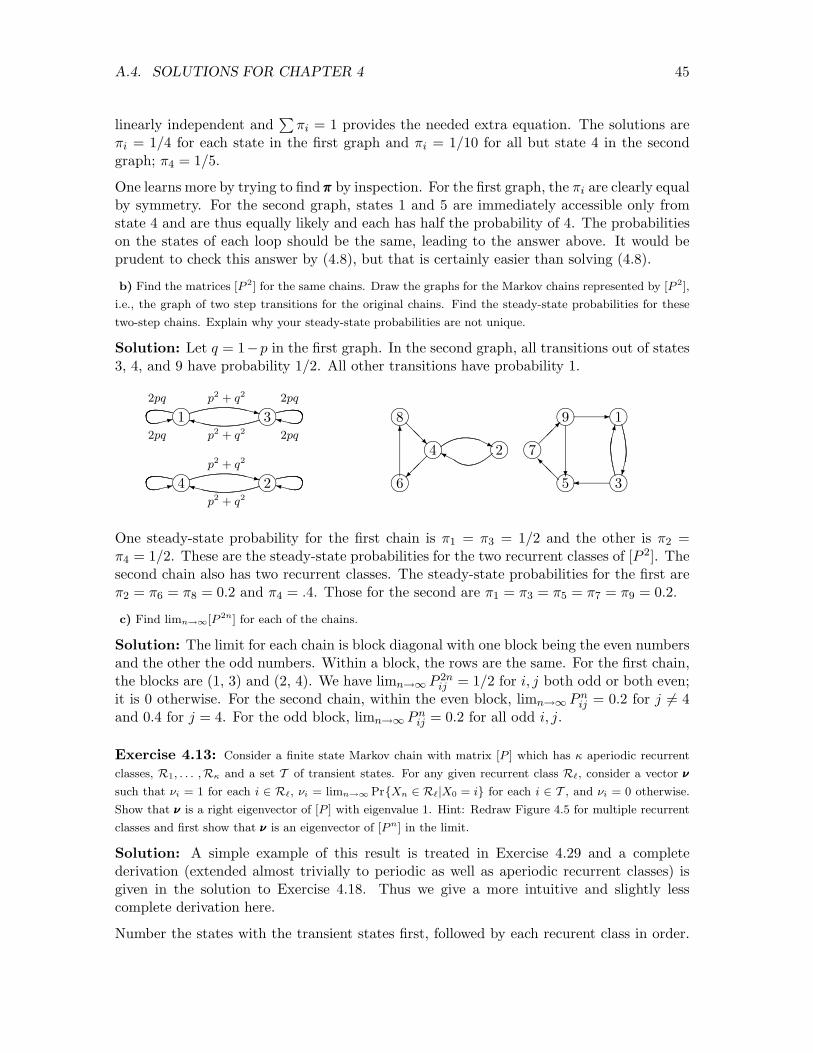
A.4. SOLUTIONS FOR CHAPTER 4 45
linearly independent andP
⇡i = 1 provides the needed extra equation. The solutions are⇡i = 1/4 for each state in the first graph and ⇡i = 1/10 for all but state 4 in the secondgraph; ⇡4 = 1/5.
One learns more by trying to find ⇡⇡⇡ by inspection. For the first graph, the ⇡i are clearly equalby symmetry. For the second graph, states 1 and 5 are immediately accessible only fromstate 4 and are thus equally likely and each has half the probability of 4. The probabilitieson the states of each loop should be the same, leading to the answer above. It would beprudent to check this answer by (4.8), but that is certainly easier than solving (4.8).
b) Find the matrices [P 2] for the same chains. Draw the graphs for the Markov chains represented by [P 2],
i.e., the graph of two step transitions for the original chains. Find the steady-state probabilities for these
two-step chains. Explain why your steady-state probabilities are not unique.
Solution: Let q = 1�p in the first graph. In the second graph, all transitions out of states3, 4, and 9 have probability 1/2. All other transitions have probability 1.
l1⇠: lXy3
l2 Xyl4⇠:
2pq
2pq
p2 + q22pq
2pq p2 + q2
p2 + q2
p2 + q2
XzXy
XzXy
l8
l6l4 HjHY
l2@@R
��
6
l9
l5@@Il7��✓
l1
l3?
⇤⌫
⇤✏
-
�
One steady-state probability for the first chain is ⇡1 = ⇡3 = 1/2 and the other is ⇡2 =⇡4 = 1/2. These are the steady-state probabilities for the two recurrent classes of [P 2]. Thesecond chain also has two recurrent classes. The steady-state probabilities for the first are⇡2 = ⇡6 = ⇡8 = 0.2 and ⇡4 = .4. Those for the second are ⇡1 = ⇡3 = ⇡5 = ⇡7 = ⇡9 = 0.2.
c) Find limn!1[P 2n] for each of the chains.
Solution: The limit for each chain is block diagonal with one block being the even numbersand the other the odd numbers. Within a block, the rows are the same. For the first chain,the blocks are (1, 3) and (2, 4). We have limn!1 P 2n
ij = 1/2 for i, j both odd or both even;it is 0 otherwise. For the second chain, within the even block, limn!1 Pn
ij = 0.2 for j 6= 4and 0.4 for j = 4. For the odd block, limn!1 Pn
ij = 0.2 for all odd i, j.
Exercise 4.13: Consider a finite state Markov chain with matrix [P ] which has aperiodic recurrent
classes, R1, . . . ,R and a set T of transient states. For any given recurrent class R`, consider a vector ⌫⌫⌫
such that ⌫i = 1 for each i 2 R`, ⌫i = limn!1 Pr{Xn 2 R`|X0 = i} for each i 2 T , and ⌫i = 0 otherwise.
Show that ⌫⌫⌫ is a right eigenvector of [P ] with eigenvalue 1. Hint: Redraw Figure 4.5 for multiple recurrent
classes and first show that ⌫⌫⌫ is an eigenvector of [P n] in the limit.
Solution: A simple example of this result is treated in Exercise 4.29 and a completederivation (extended almost trivially to periodic as well as aperiodic recurrent classes) isgiven in the solution to Exercise 4.18. Thus we give a more intuitive and slightly lesscomplete derivation here.
Number the states with the transient states first, followed by each recurent class in order.
46 APPENDIX A. SOLUTIONS TO EXERCISES
Then [P ] has the following block structure
[P ] =
2666664
[PT ] [PT R1 ]. . . . . . [PT R ]
0 [PR1 ] 0. . . 0
. . . . . . . . . . . . . . .
0 0. . . 0 [PR ]
3777775
.
The `th recurrent class has an |R`| by |R`| transition matrix which, viewed alone, hasan eigenvalue � = 1 of multiplicity 1, a corresponding unique (within a scale factor) lefteigenvector, say ⇡⇡⇡(R`), and a corresponding unique (within a scale factor) right eigenvector,⌫⌫⌫(R`) = (1, . . . , 1)T (see Theorem 4.4.2).
Let ⇡⇡⇡(`) be an M dimensional row vector whose components are equal to those of ⇡⇡⇡(R`) overthe states of R` and equal to 0 otherwise. Then it can be seen by visualizing elementaryrow/matrix multiplication on the block structure of [P ] that ⇡⇡⇡(`)[P ] = ⇡⇡⇡(`). This gives us left eigenvectors of eigenvalue 1, one for each recurrent class R`.
These left eigenvectors are clearly linearly independent and span the dimensional spaceof left eigenvectors of eigenvalue 1 (see Exercise 4.18).
If there are no transient states, then a set of right eigenvectors can be chosen in the sameway as the left eigenvectors. That is, for each `, 1 ` , the components of ⌫⌫⌫(`) canbe chosen to be 1 for each state in R` and 0 for all other states. This doesn’t satisfy theeigenvector equation if there are transient states, however. We now show, instead, that foreach `, 1 ` , there is a right eigenvector ⌫⌫⌫(`) of eigenvalue 1 that can be nonzero bothon R` and T . such that ⌫(`)
i = 0 for all i 2 Rm, for each m 6= `. Finally we will show thatthese vectors are linearly independent and have the properties specified in the problemstatement.
The right eigenvector equation that must be satisfied by ⌫⌫⌫(`) assuming that ⌫(`)i 6= 0 only
for i 2 R` [ T can be written out component by component, getting
⌫(`)i =
Xj2R`
Pij⌫(`)j for i 2 R`
⌫(`)i =
Xj2T
Pij⌫(`)j +
Xj2R`
Pij⌫(`)j for i 2 T .
The first set of equations above are simply the usual right eigenvector equations for eigen-value 1 over the recurrent submatrix [PR` ]. Thus ⌫(`)
j = 1 for j 2 R` and this solution(over R`) is unique within a scale factor. Substituting this solution into the second set ofequations, we get
⌫(`)i =
Xj2T
Pij⌫(`)j +
Xj2R`
Pij for i 2 T .
This has a unique solution for each ` (see Exercise 4.18). These eigenvectors, {⌫⌫⌫(`), 1 ` } must be linearly independent since ⌫(`)
i = 1 for i 2 R` and ⌫(`)i = 0 for i 2 Rm, m 6= `.
They then form a basis for the dimensional space of eigenvectors of [P ] of eigenvalue 1.

A.4. SOLUTIONS FOR CHAPTER 4 47
These eigenvectors are also eigenvectors of eigenvalue 1 for [Pn] for each n > 1. Thus
⌫(`)i =
Xj2T
Pnij⌫
(`)j +
Xj2R`
Pnij for i 2 T .
Now recall that for i, j 2 T , we have limn!1 Pnij = 0. Also
Pj2R`
Pnij is the probability
that Xn 2 R` given X0 2 T . Since there is no exit from R`, this quantity is non-decreasingin n and bounded by 1, so it has a limit. This limit is the probability of ever going from ito R`, completing the derivation.
Exercise 4.14: Answer the following questions for the following stochastic matrix [P ]
[P ] =
24 1/2 1/2 0
0 1/2 1/20 0 1
35 .
a) Find [P n] in closed form for arbitrary n > 1.
Solution: There are several approaches here. We first give the brute-force solution ofsimply multiplying [P ] by itself multiple times (which is reasonable for a first look), andthen give the elegant solution.
[P 2] =
24 1/2 1/2 0
0 1/2 1/20 0 1
3524 1/2 1/2 0
0 1/2 1/20 0 1
35 =
24 1/4 2/4 1/4
0 1/4 3/40 0 1
35 .
[P 3] =
24 1/2 1/2 0
0 1/2 1/20 0 1
3524 1/4 2/4 1/4
0 1/4 3/40 0 1
35 =
24 1/8 3/8 4/8
0 1/8 7/80 0 1
35 .
We could proceed to [P 4], but it is natural to stop and think whether this is telling ussomething. The bottom row of [Pn] is clearly (0, 0, 1) for all n, and we can easily eitherreason or guess that the first two main diagonal elements are 2�n. The final column iswhatever is required to make the rows sum to 1. The only questionable element is Pn
12. Weguess that it is n2�n and verify it by induction,
[Pn+1] = [P ] [Pn] =
24 1/2 1/2 0
0 1/2 1/20 0 1
3524 2�n n2�n 1� (n+1)2�n
0 2�n 1� 2�n
0 0 1
35
=
24 2�n�1 (n+1)2�n�1 1� (n+2)2�n�1
0 2�n 1� 2�n
0 0 1
35 .
This solution is not very satisfying, first because it is tedious, second because it required asomewhat unmotivated guess, and third because no clear rhyme or reason emerged.
The elegant solution, which can be solved with no equations, requires looking at the graphof the Markov chain,

48 APPENDIX A. SOLUTIONS TO EXERCISES
1 2 3n1/2 1/2
1/21/2 1O O O
n Xz n Xz
It is now clear that Pn11 = 2�n is the probability of taking the lower loop for n successive
steps starting in state 1. Similarly Pn22 = 2�n is the probability of taking the lower loop at
state 2 for n successive steps.
Finally, Pn12 is the probability of taking the transition from state 1 to 2 exactly once out
the n transitions starting in state 1 and of staying in the same state (first 1 and then 2)for the other n � 1 transitions. There are n such paths, corresponding to the n possiblesteps at which the 1 ! 2 transition can occur, and each path has probability 2�n. ThusPn
12 = n2�n, and we ‘see’ why this factor of n appears. The transitions Pni3 are then chosen
to make the rows sum to 1, yielding the same solution as above.
b) Find all distinct eigenvalues and the multiplicity of each distinct eigenvalue for [P ].
Solution: Note that [P ] is an upper triangular matrix, and thus [P � �I] is also uppertriangular. Thus its determinant is the product of the terms on the diagonal, det[P � ⇤I] =(12 � �)2(1 � �). It follows that � = 1 is an eigenvalue of multiplicity 1 and � = 1/2 is an
eigenvalue of multiplicity 2.
c) Find a right eigenvector for each distinct eigenvalue, and show that the eigenvalue of multiplicity 2 does
not have 2 linearly independent eigenvectors.
Solution: For any Markov chain, e = (1, . . . , 1)T is a right eigenvector. For the givenchain, this is unique within a scale factor, since � = 1 has multiplicity 1. For ⌫⌫⌫ to be a righteigenvector of eigenvalue 1/2, it must satisfy
12⌫1 +
12⌫2 + 0⌫3 =
12⌫1
0⌫1 +12⌫2 +
12⌫3 =
12⌫2
⌫3 =12⌫3.
From the first equation, ⌫2 = 0 and from the third ⌫3 = 0, so ⌫⌫⌫ = (1, 0, 0) is the righteigenvector of � = 1/2, unique within a scale factor. Thus � = 1/2 does not have 2 linearlyindependent eigenvectors.
d) Use (c) to show that there is no diagonal matrix [⇤] and no invertible matrix [U ] for which [P ][U ] = [U ][⇤].
Solution: Letting ⌫⌫⌫1,⌫⌫⌫2,⌫⌫⌫3 be the columns of an hypothesized matrix [U ], we see that[P ][U ] = [U ][⇤] can be written out as [P ]⌫⌫⌫i = �i⌫⌫⌫i for i = 1, 2, 3. For [U ] to be invertible,⌫⌫⌫1,⌫⌫⌫2,⌫⌫⌫3 must be linearly independent eigenvectors of [P ]. However part (c) showed that3 such eigenvectors do not exist.
e) Rederive the result of (d) using the result of a) rather than c).
Solution: If the [U ] and [⇤] of (d) exist, then [Pn] = [U ][⇤n][U�1]. Then, as in (4.30),[Pn] =
P3i=1 �n
i ⌫⌫⌫(i)⇡⇡⇡(i) where ⌫⌫⌫(i) is the ith column of [U ] and ⇡⇡⇡(i) is the ith row of [U�1].

A.4. SOLUTIONS FOR CHAPTER 4 49
Since Pn12 = n(1/2)n, the factor of n means that it cannot have the form a�n
1 + b�n2 + c�n
3for any choice of �1,�2,�3, a, b, c.
Note that the argument here is quite general. If [Pn] has any terms containing a polynomialin n times �n
i , then the eigenvectors can’t span the space and a Jordan form decompositionis required.
Exercise 4.16: a) Let � be an eigenvalue of a matrix [A], and let ⌫⌫⌫ and ⇡⇡⇡ be right and left eigenvectorsrespectively of �, normalized so that ⇡⇡⇡⌫⌫⌫ = 1. Show that
[[A]� �⌫⌫⌫⇡⇡⇡]2 = [A2]� �2⌫⌫⌫⇡⇡⇡.
Solution: We simply multiply out the original square,
[[A]� �⌫⌫⌫⇡⇡⇡]2 = [A2]� �⌫⌫⌫⇡⇡⇡[A]� �[A]⌫⌫⌫⇡⇡⇡ + �2⌫⌫⌫⇡⇡⇡⌫⌫⌫⇡⇡⇡
= [A2]� �2⌫⌫⌫⇡⇡⇡ � �2⌫⌫⌫⇡⇡⇡ + �2⌫⌫⌫⇡⇡⇡ = [A2]� �2⌫⌫⌫⇡⇡⇡.
b) Show that⇥[An]� �n⌫⌫⌫⇡⇡⇡
⇤ ⇥[A]� �⌫⌫⌫⇡⇡⇡
⇤= [An+1]� �n+1⌫⌫⌫⇡⇡⇡.
Solution: This is essentially the same as (a)⇥[An]� �n⌫⌫⌫⇡⇡⇡
⇤ ⇥[A]� �⌫⌫⌫⇡⇡⇡
⇤= [An+1]� �n⌫⌫⌫⇡⇡⇡[A]� �[An]⌫⌫⌫⇡⇡⇡ + �n+1⌫⌫⌫⇡⇡⇡⌫⌫⌫⇡⇡⇡
= [An+1]� �n+1⌫⌫⌫⇡⇡⇡.
c) Use induction to show that [[A]� �⌫⌫⌫⇡⇡⇡]n = [An]� �n⌫⌫⌫⇡⇡⇡.
Solution: (a) gives the base of the induction and (b) gives the inductive step.
Exercise 4.21: Suppose A and B are each ergodic Markov chains with transition probabilities {PAi,Aj}and {PBi,Bj} respectively. Denote the steady-state probabilities of A and B by {⇡Ai} and {⇡Bi} respectively.The chains are now connected and modified as shown below. In particular, states A1 and B1 are nowconnected and the new transition probabilities P 0 for the combined chain are given by
P 0A1,B1 = ", P 0A1,Aj= (1� ")PA1,Aj for all Aj
P 0B1,A1 = �, P 0B1,Bj= (1� �)PB1,Bj for all Bj .
All other transition probabilities remain the same. Think intuitively of " and � as being small, but do notmake any approximations in what follows. Give your answers to the following questions as functions of ", �,{⇡Ai} and {⇡Bi}.
n XzXyA1 B1
nn
nn
⇢⇢⇢
ZZZ
ZZZ
⇢⇢⇢
nn
nnZZZ
⇢⇢⇢�
���� "
�
'
&
$
%
'
&
$
%Chain A Chain B
a) Assume that ✏ > 0, � = 0 (i.e., that A is a set of transient states in the combined chain). Starting in
state A1, find the conditional expected time to return to A1 given that the first transition is to some state
in chain A.

50 APPENDIX A. SOLUTIONS TO EXERCISES
Solution: Conditional on the first transition from state A1 being to a state Ai 6= A1, theseconditional transition probabilities are the same as the original transition probabilities forA. If we look at a long sequence of transitions in chain A alone, the relative frequencyof state A1 tends to ⇡A1 so we might hypothesize that, within A, the expected time toreturn to A1 starting from A1 is 1/⇡A1 . This hypothesis is correct and we will verify it bya simple argument when we study renewal theory. Here, however, we verify it by lookingat first-passage times within the chain A. For now, label the states in A as (1, 2, . . . ,M)where 1 stands for A1. For 2 i M, let vi be the expected time to first reach state 1starting in state i. As in (4.31),
vi = 1 +Xj 6=1
Pijvj ; 2 i M. (A.15)
We can use these equations to write an equation for the expected time T to return to state1 given that we start in state 1. The first transition goes to each state j with probabilityP1j and the remaining time to reach state 1 from state j is vj . We define v1 = 0 since ifthe first transition from 1 goes to 1, there is no remaining time required to return to stateA1. We then have
T = 1 +MX
j=1
Pijvj . (A.16)
Note that this is very di↵erent from (4.32) where [P ] is a Markov chain in which 1 is atrapping state. We can now combine (A.16) (for component 1) and (A.15) (for components2 to M) into the following vector equation:
Te1 + v = e + [P ]v ,
where e1 = (1, 0, 0, . . . , 0)T and e = (1, 1, . . . , 1)T. Motivated by the hypothesis thatT = 1/⇡1, we premultiply this vector equation by the steady-state row vector ⇡⇡⇡, getting
T⇡1 + ⇡⇡⇡v = 1 + ⇡⇡⇡[P ]v = 1 + ⇡⇡⇡v .
Cancelling ⇡⇡⇡v from each side, we get T = 1/⇡1 as hypothesized.
b) Assume that ✏ > 0, � = 0. Find TA,B, the expected time to first reach state B1 starting from state A1.
Your answer should be a function of ✏ and the original steady-state probabilities {⇡Ai} in chain A.
Solution: Starting in state A1, we reach B1 in a single step with probability ✏. Withprobability 1� ✏, we wait for a return to A1 and then have expected time TA,B remaining.Thus TA,B = ✏ + (1� ✏)
�1
⇡A1+ TA,B
�. Solving this equation,
TA,B = 1 +1� ✏
✏⇡A1
.
c) Assume " > 0, � > 0. Find TB,A, the expected time to first reach state A1, starting in state B1. Your
answer should depend only on � and {⇡Bi}.

A.4. SOLUTIONS FOR CHAPTER 4 51
Solution: The fact that ✏ > 0 here is irrelevant since that transition can never be used inthe first passage from B1 to A1. Thus the answer is the reversed version of the answer to(b), where now ⇡B1 is the steady-state probability of B1 for chain B alone.
TB,A = 1 +1� �
�⇡B1
.
d) Assume " > 0 and � > 0. Find P 0(A), the steady-state probability that the combined chain is in one of
the states {Aj} of the original chain A.
Solution: With 0 < ✏ < 1 and 0 < � < 1, the combined chain is ergodic. To see this, notethat all states communicate with each other so the combined chain is recurrent. Also, allwalks in A are still walks in the combined chain, so the gcd of their lengths is 1. Thus A,and consequently B, are still aperiodic.
We can thus use the steady state equations to find the unique steady-state vector ⇡⇡⇡. Inparts (d), (e), and (f), we are interested in those probabilities in chain A. We denote thosestates, as before, as (1, . . . ,M) where 1 is state A1. Steady-state probabilities for A in thecombined chain for given ✏, � are denoted ⇡0j , whereas they are denoted as ⇡j in the originalchain. We first find ⇡01 and then ⇡0j for 2 j M.
As we saw in (a), the expected first return time from a state to itself is the reciprocal ofthe steady-state probability, so we first find TAA, the expected time of first return fromA1 to A1. Given that the first transition from state 1 goes to a state in A, the expectedfirst-return time is 1/⇡1 from (a). If the transition goes to B1, the expected first-returntime is 1 + TBA, where TBA is found in (c). Combining these with the a priori probabilitiesof going to A or B,
TAA = (1� ✏)/⇡1 + ✏⇥1 + TBA
⇤=
1� ✏
⇡1+ 2✏ +
✏(1� �)�⇡B1
.
Thus
⇡01 =1� ✏
⇡1+ 2✏ +
✏(1� �)�⇡B1
��1
.
Next we find ⇡0j for the other states in A in terms of the ⇡j for the uncombined chains and⇡01. The original and the combined steady-state equations for 2 j M are
⇡j =Xi6=1
⇡iPij + ⇡1P1j ; ⇡0j =Xi6=1
⇡0iPij + ⇡01(1� ✏)P1j .
These equations, as M�1 equations in the unknowns ⇡j ; j � 2 for given ⇡1, uniquely specify⇡2, . . . ,⇡M and they di↵er in ⇡1 being replaced by (1 � ✏)⇡01. From this, we see that thesecond set of equations is satisfied if we choose
⇡0j = ⇡j(1� ✏)⇡01
⇡1.
We can now sum the steady-state probabilities in A to get
Pr{A} =MX
j=1
⇡0j = ⇡01
✏ +
1� ✏
⇡1
�.

52 APPENDIX A. SOLUTIONS TO EXERCISES
e) Assume " > 0, � = 0. For each state Aj 6= A1 in A, find vAj , the expected number of visits to state Aj ,
starting in state A1, before reaching state B1. Your answer should depend only on " and {⇡Ai}.
Solution: We use a variation on the first passage time problem in (a) to find the expectednumber of visits to state j, E [Nj ], in the original chain starting in state 1 before the firstreturn to 1. Here we let vi(j) be the expected number of visits to j, starting in state i,before the first return to 1. The equations are
E [Nj ] =Xk 6=1
P1kvk(j) + P1j ; vi(j) =Xk 6=1
Pikvk(j) + Pij for i 6= 1.
The first equation represents E [N(j)] in terms of the expected number of visits to j con-ditional on each first transition k from the initial state 1. in the special case where thatfirst transition is to j, the expected number of visits to j includes both 1 for the initial visitplus vj(j) for the subsequent visits. The second set of equations are similar, but give theexpected number of visits to j (before a return to 1) starting from each state other than 1.
Writing this as a vector equation, with v(j) = (0, v2(j), v3(j). . . . , vM(j))T, we get
E [Nj ] e1 + v(j) = [P ]v(j) + [P ]ej .
Note that [P ]ej is the column vector (p1j , . . . , PMj)T Premultiplying by ⇡⇡⇡, we see thatE [Nj ] = ⇡j/⇡1. Finally, to find vAj , the expected number of visits to state j before the firstto B1, we have
vAj = (1� ✏)[E [Nj ] + vAj ] =(1� ✏)E [Nj ]
✏=
(1� ✏)⇡j
✏⇡i.
f) Assume " > 0, � > 0. For each state Aj in A, find ⇡0Aj, the steady-state probability of being in state Aj
in the combined chain. Hint: Be careful in your treatment of state A1.
Solution: This was solved in (d). Readers might want to come back to this exercise laterand re-solve it more simply using renewal theory.
Exercise 4.22: Section 4.5.1 showed how to find the expected first passage times to a fixed state, say1, from all other states. It is often desirable to include the expected first recurrence time from state 1 toreturn to state 1. This can be done by splitting state 1 into 2 states, first an initial state with no transitionscoming into it but the original transitions going out, and second, a final trapping state with the originaltransitions coming in.
a) For the chain on the left side of Figure 4.6, draw the graph for the modified chain with 5 states where
state 1 has been split into 2 states.
Solution: We split state 1 into states 10 and 1, where 10 is the trapping state and 1 can bean initial state.
�⇡
HY
�*Hj
⇤⌫
⇤✏
�*
Hj
⇠: Xyn nn
n1 3
4
2
n10 �� @I

A.4. SOLUTIONS FOR CHAPTER 4 53
b) Suppose one has found the expected first-passage-times vj for states j = 2 to 4 (or in general from 2 to
M). Find an expression for v1, the expected first recurrence time for state 1 in terms of v2, v3, . . . vM and
P12, . . . , P1M.
Solution: Note that v2, v3, and v4 are unchanged by the addition of state 1, since notransitions can go to 1 from states 2, 3, or 4. We then have
v1 = 1 +4X
j=2
P1jvj .
Exercise 4.23: a) Assume throughout that [P ] is the transition matrix of a unichain (and thus the
eigenvalue 1 has multiplicity 1). Show that a solution to the equation [P ]w �w = r � ge exists if and only
if r � ge lies in the column space of [P � I] where [I] is the identity matrix.
Solution: Let C[P � I] be the column space of [P � I]. A vector x is in C[P � I] if x is alinear combination of columns of [P�I), i.e., if x is w1 times the first column of [P�I] plusw2 times the second column, etc. More succinctly, x 2 C[P � I] if and only if x = [P � I]wfor some vector w . Thus r � ge 2 C[P � I] if and only if [P � I]w = r � ge for some w ,which after rearrangement is what is to be shown.
b) Show that this column space is the set of vectors x for which ⇡⇡⇡x = 0. Then show that r � ge lies in this
column space.
Solution: We know that [P ] has a single eigenvalue equal to 1. Thus [P �I] is singular andthe steady-state vector ⇡⇡⇡ satisfies ⇡⇡⇡[P �I] = 0. Thus for every w , ⇡⇡⇡[P �I]w = 0 so ⇡⇡⇡x = 0for every x 2 C[P � I] . Furthermore, ⇡⇡⇡ (and its scalar multiples) are the only vectors tosatisfy ⇡⇡⇡[P � I] = 0 and thus C[P � I] is an M � 1 dimensional vector space. Since thevector space of vectors x that satisfy ⇡⇡⇡x = 0 is M� 1 dimensional, this must be the sameas C[P � I]. Finally, since g is defined as ⇡⇡⇡r , we have ⇡⇡⇡(r � ge) = 0, so r � ge 2 C[P � I].
c) Show that, with the extra constraint that ⇡⇡⇡w = 0, the equation [P ]w�w = r�ge has a unique solution.
Solution: For any w 0 that satisfies [P ]w 0 � w 0 = r � ge, it is easy to see that w 0 + ↵ealso satisfies this equation for any real ↵. Furthermore, since the column space of [P � I]is M � 1 dimensional, this set of solutions, namely {w 0 + ↵e; ↵ 2 <} is the entire set ofsolutions. The additional constraint that ⇡⇡⇡(w 0 + ↵e) = ⇡⇡⇡w 0 + ↵ = 0 specifies a uniqueelement in this set.
Exercise 4.24: For the Markov chain with rewards in Figure 4.8,
a) Find the solution to (4.37) and find the gain g.
Solution: The symmetry in the transition probabilities shows that ⇡⇡⇡ = (1/2, 1/2)T, andthus g = ⇡⇡⇡r = 1/2. The first component of (4.37), i.e., of www + ge = [P ]w + r is thenw1 + 1/2 = P11w1 + P12w2 + r1. This simplifies to w1 �w2 = �50. The second componentis redundant, and ⇡⇡⇡w = 0 simplifies to w1 + w2 = 0. Thus w1 = �25 and w2 = 25.
b) Modify Figure 4.8 by letting P12 be an arbitrary probability. Find g and w again and give an intuitive
explanation of why P12 e↵ects w2.

54 APPENDIX A. SOLUTIONS TO EXERCISES
Solution: With arbitrary P12, the steady-state probabilities become
⇡1 =0.01
P12 + 0.01; ⇡2 =
P12
P12 + 0.01.
The steady-state gain, g = ⇡⇡⇡r , then becomes g = P12/(P12 +0.01). Solving for w as before,we get
w1 =�P12
(P12 + 0.01)2w2 =
0.01(P12 + 0.01)2
.
As P12 increases, the mean duration of each visit to state 1 decreases so that the fraction oftime spent in state 1 also decreases, thus increasing the expected gain. At the same time,the relative advantage of starting in state 2 decreases since the interruptions to having areward on each transition become shorter. For example, if P12 = 1/2, the mean time toleave state 1, starting in state 1, is 2.
Exercise 4.26: Consider the Markov chain below:
3
1
2
kk
k
⇣⇣⇣⇣⇣⇣⇣⇣⇣1
PPPPPPPPPq
6 1/2
1/4
1/2 1
1/2
1/4
Xy
⇠:
⇠:
a) Suppose the chain is started in state i and goes through n transitions; let vi(n) be the expected number
of transitions (out of the total of n) until the chain enters the trapping state, state 1. Find an expression
for v(n) = (v1(n), v2(n), v3(n))T in terms of v(n� 1) (take v1(n) = 0 for all n). (Hint: view the system as
a Markov reward system; what is the value of r?)
Solution: We use essentially the same approach as in Section 4.5.1, but we are explicithere about the number of transitions. Starting in any state i 6= 1 with n transitions to go,the expected number of transitions until the first that either enters the trapping state orcompletes the nth transition is given by
vi(n) = 1 +3X
j=1
Pijvj(n�1). (A.17)
Since i = 1 is the trapping state, we can express v1(n) = 0 for all n, since no transitions arerequired to enter the trapping state. Thus (A.17) is modified to v1(n) =
P3j=1 P1jvj(n�1)
for i = 1. Viewing r as a reward vector, with one unit of reward for being in any state otherthan the trapping state, we have r = (0, 1, 1)T. Thus (A.17) can be expressed in vectorform as
v(n) = r + [P ]v(n� 1).
b) Solve numerically for limn!1 v(n). Interpret the meaning of the elements vi in the solution of (4.32).

A.4. SOLUTIONS FOR CHAPTER 4 55
Solution: We have already seen that v1(n) = 0 for all n, and thus, since P23 = 0, we havev2(n) = 1 + (1/2)v2(n�1). Since v2(0) = 0, this iterates to
v2(n) = 1 +12�1 + v2(n�2)
�= 1 +
12
+14�1 + v2(n�3)
�= · · · = 2� 2�(n�1).
For v3(n), we use the same approach, but directly use the above solution for v2(n) for eachn.
v3(n) = 1 + P32v2(n�1) + P33v3(n�1) = 1 +12�1� 2�(n�2)
�+
14v3(n�1)
= (2� 2n�1) +14
h2� 2n�2 +
14v3(n�2)
i= · · ·
= (2� 2n�1) +14
h2� 2n�2
i+
116
h2� 2n�3
i+ · · ·+ 1
4n�1[2� 20]
= 2h1 +
14
+142
+ · · · 14n�1
i�h2�(n�1) + 2�n + · · ·+ 2�2n+2
i
= 21� 4�n
1� 4�1
�� 2�(n�1)
1� 2�n
1� 2�1
�=
83� 2�2n+3
3� 2�n+2 + 2�2n+2.
Taking the limit,
limn!1
v2(n) = 2; limn!1
v3(n) =83.
c) Give a direct argument why (4.32) provides the solution directly to the expected time from each state
to enter the trapping state.
Solution: The limit as n !1 gives the expected time to enter the trapping state with nolimit on the required number of transitions. This limit exists in general since the transientstates persist with probabilities decreasing exponentially with n.
Exercise 4.28: Consider finding the expected time until a given string appears in an IID binary sequence
with Pr{Xi=1} = p1, Pr{Xi=0} = p0 = 1� p1.
a) Following the procedure in Example 4.5.1, draw the 3 state Markov chain for the string (0, 1). Find the
expected number of trials until the first occurrence of that string.
Solution:
l0 Xz l1 Xz l2⇠:
p1 ✏Xy
p0
p0p1 1
Let vi be the expected first-passage time from node i to node 2. Then
v0 = 1 + p1v0 + p0v1; v1 = 1 + p0v1 + p1v2
v0 = 1/p0 + v1; v1 = 1/p1 + v2.
Combining these equations to eliminate v1,
v0 = 1/p0 + 1/p1 + v2 = 1/p0p1 + v2.

56 APPENDIX A. SOLUTIONS TO EXERCISES
Finally, the trapping state, 2, is reached when the string 01 first occurs, so v2 = 0 andv0 = 1/p0p1.
b) For parts b) to d), let (a1, a2, a3, . . . , ak) = (0, 1, 1, . . . , 1), i.e., zero followed by k � 1 ones. Draw the
corresponding Markov chain for k = 4.
Solution:
0 1 2 3 4⇠: n Xz n Xz n Xz n Xz nXyXyHYO p0
0111011010 p1p1p1p0p11
p0p0
c) Let vi, 1 i k be the expected first-passage time from state i to state k. Note that vk = 0. For each
i, 1 i < k, show that vi = ↵i + vi+1 and v0 = �i + vi+1 where ↵i and �i are each expressed as a product
of powers of p0 and p1. Hint: use induction on i using i = 1 as the base. For the inductive step, first find
�i+1 as a function of �i starting with i = 1 and using the equation v0 = 1/p0 + v1.
Solution: (a) solved the problem for i = 1. The fact that the string length was 2 therewas of significance only at the end where we set v2 = 0. We found that ↵1 = 1/p1 and�1 = 1/p0p1.
For the inductive step, assume vi = ↵i + vi+1 and v0 = �i + vi+1 for a given i � 1. Usingthe basic first-passage-time equation,
vi+1 = 1 + p0v1 + p1vi+2
= p0v0 + p1vi+2
= p0�i + p0vi+1 + p1vi+2.
The second equality uses the basic equation for v0, i.e., v0 = 1 + p1v0 + p0v1 which reducesto p0v1 + 1 = p0v0 and the third equality uses the inductive hypothesis v0 = �i + vi+1.Combining the terms in vi+1,
vi+1 =p0�i
p1+ vi+2.
This completes half the inductive step, showing that ai+1 = p0�i/p1. Now we use this resultplus the inductive hypothesis v0 = �i + vi+1 to get
v0 = �i + vi+1 = �i +p0�i
p1+ vi+2 =
�i
p1+ vi+2.
This completes the second half of the induction, showing that �i+1 = �i/p1. Iterating onthese equations for �i and ↵i, we find the explicit expression
↵i =1pi1
; �i =1
p0pi1
.
Note that the algebra here was quite simple, but if one did not follow the hints precisely,one could get into a terrible mess. In addition, the whole thing was quite unmotivated. We

A.4. SOLUTIONS FOR CHAPTER 4 57
view the occurrence of these strings as renewals in Exercise 5.35 and find a more intuitiveway to derive the same answer.
d) Let a = (0, 1, 0). Draw the corresponding Markov chain for this string. Evaluate v0, the expected time
for (0, 1, 0) to occur.
Solution:
0 1 2 3⇠: n Xz n Xz n Xz nXy 1HY
✏
p1
010010 p0p1p0p1
p0
The solution for v0 and v1 in terms of v2 is the same as (a). The basic equation for v2 interms of its outward transitions is
v2 = 1 + p0v0 + p1v3
= 1 + p0
1
p0p1+ v2
�.
Combining the terms in v2, we get
p1v2 = 1 + 1/p1.
Using v0 = 1/p0p1 + v2,
v0 =1
p21p0
+1p1
+1p21
=1p1
+1
p0p21
.
This solution will become more transparent after doing Exercise 5.35.
Exercise 4.29: a) Find limn!1[P n] for the Markov chain below. Hint: Think in terms of the long termtransition probabilities. Recall that the edges in the graph for a Markov chain correspond to the positivetransition probabilities.
n1 n3 n2� -
CO
P31 P32
P33
11Xy⇠:
Solution: The chain has 2 recurrent states, each in its own class, and one transient state.Thus limn!1 Pn
11 = 1 and limn!1 Pn22 = 1. Let q1 = limn!1 Pn
31 and q2 = limn!1 Pn32.
Since q1 + q2 = 1 and since in each transition starting in state 3, P31 and P32 give theprobabilities of moving to 1 or 2, q1 = P31/(P31 +P32) and q2 = P32/(P31 +P32). The otherlong term transtion probabilities are zero, so
limn!1
[Pn] =
24 1 0 0
0 1 0q1 q2 0
35 .
The general case here, with an arbitrary set of transient states and an arbitrary number ofrecurrent classes is solved in Exercise 4.18.

58 APPENDIX A. SOLUTIONS TO EXERCISES
b) Let ⇡⇡⇡(1) and ⇡⇡⇡(2) denote the first two rows of limn!1[P n] and let ⌫⌫⌫(1) and ⌫⌫⌫(2) denote the first two
columns of limn!1[P n]. Show that ⇡⇡⇡(1) and ⇡⇡⇡(2) are independent left eigenvectors of [P ], and that ⌫⌫⌫(1) and
⌫⌫⌫(2) are independent right eigenvectors of [P ]. Find the eigenvalue for each eigenvector.
Solution: ⇡⇡⇡(1) = (1, 0, 0) and ⇡⇡⇡(2) = (0, 1, 0). Multiplying ⇡⇡⇡(i) by limn!1[Pn] for i = 1, 2we see that these are the left eigenvectors of eigenvalue 1 of the two recurrent classes. Wealso know this from Section 4.4. Similarly, ⌫⌫⌫(1) = (1, 0, q1)T and ⌫⌫⌫(2) = (0, 1, q2)T are righteigenvectors of eigenvalue 1, both of limn!1[Pn] and also of [P ].
c) Let r be an arbitrary reward vector and consider the equation
w + g(1)⌫⌫⌫(1) + g(2)⌫⌫⌫(2) = r + [P ]w . (A.18)
Determine what values g(1) and g(2) must have in order for (A.18) to have a solution. Argue that with the
additional constraints w1 = w2 = 0, (A.18) has a unique solution for w and find that w .
Solution: In order for this equation to have a solution, it is necessary, first, for a solutionto exist when both sides are premultiplied by ⇡⇡⇡(1). This results in g(1) = r1. Similarly,premultiplying by ⇡⇡⇡(2) results in g(2) = r2. In other words, g(1) is the gain per transitionwhen in state 1 or when the chain moves fom state 3 to state 1. Similarly g(2) is the gainper transition in state 2 or after a transition from 3 to 2. Since there are two recurrent setsof states, there is no common meaning to a gain per transition.
Setting w1 = w2 = 0 makes a certain amount of sense, since starting in state 1 or startingin state 2, the reward increases by r1 or r2 per transition with no initial transient. Withthis choice, the first two components of the vector equation in (A.18) are 0=0 and the thirdis
w3 + r3q1 + r2q2 = r3 + P33w3.
Solving for w3,
w3 =1
P31 + P32
r3 � r1
P31
P31 + P32� r2
P32
P31 + P32
�.
This can be interpreted as the relative gain of starting in state 3 relative to the ‘average’of starting in 1 or 2. The interpretation is quite limited, since the gain per transitiondepends on which recurrent class is entered, and thus relative gain has nothing definitivefor comparison.
Exercise 4.32: George drives his car to the theater, which is at the end of a one-way street. There areparking places along the side of the street and a parking garage that costs $5 at the theater. Each parkingplace is independently occupied or unoccupied with probability 1/2. If George parks n parking places awayfrom the theater, it costs him n cents (in time and shoe leather) to walk the rest of the way. George ismyopic and can only see the parking place he is currently passing. If George has not already parked by thetime he reaches the nth place, he first decides whether or not he will park if the place is unoccupied, andthen observes the place and acts according to his decision. George can never go back and must park in theparking garage if he has not parked before.
a) Model the above problem as a 2 state dynamic programming problem. In the “driving” state, state
2, there are two possible decisions: park if the current place is unoccupied or drive on whether or not the
current place is unoccupied.

A.4. SOLUTIONS FOR CHAPTER 4 59
Solution: View the two states as walking (state 1) and driving (state 2). The statetransitions correspond to passing successive possibly idle parking spaces, which are passedeither by car or foot. Thus r1 = 1 (the cost in shoe leather and time) and r2 = 0. Thereis no choice of policy in state 1, but in state 2, policy t is to try to park and policy d iscontinue to drive.
First consider stage 1 where George is between the second and first parking space from theend. If George is in the walk state, there is one unit of cost going from 2 to 1 and 1 unitof final cost going from 1 to 0. If George is in the drive state (2) and uses the try policy,r2 = 0 and with probability 1/2, he parks and has one unit final cost getting to the theatre.With probability 1/2, he doesn’t park and the final cost is 500. For policy d, r2 = 0 andwith probability 1, the final cost is 500.
In summary, u = (1, 500)T, r = (0, 1)T and the Markov chain with the t and d policies instate 2 is
1 2 1 21
P (d)22 P (t)
22
r1=1 r2=0
1P (t)
22
1/2r1=1 r2=0
1Xy⇠: n
Xyn nn⇠: Xy
1/2
b) Find v⇤i (n,u), the minimum expected aggregate cost for n stages (i.e., immediately before observation
of the nth parking place) starting in state i = 1 or 2; it is su�cient to express v⇤i (n,u) in terms of v⇤i (n�1).
The final costs, in cents, at stage 0 should be v2(0) = 500, v1(0) = 0.
Solution: We start with stage 1.
v⇤(1,u) = r + mink
[P k ]u = (2, 250.5)T,
where policy t is clearly optimal. At an arbitrary stage n, the cost is found iteratively fromstage n� 1 by (4.48), i.e.,
v⇤(n,u) = minkkk
⇣rkkk + [Pkkk]v⇤(n� 1,u)
⌘. (A.19)
c) For what values of n is the optimal decision the decision to drive on?
Solution: The straightforward approach (particularly with computional aids is to simplycalculate (A.19). The cost drops sharply with increasing n and for n � 8, the optimaldecision is to drive on, whereas for n 7, the optimal decision is to park if possible.
As with many problems, the formalism of dymamic programming makes hand calculationand understanding more awkward than it need be. The simple approach, for any distancen away from the theatre, is to simply calculate the cost of parking if a place is available,namely n, and to calculate the expected cost if one drives on. This expected cost, En iseasily seen to be
En =12(m� 1) +
14(m� 2) + · · ·+ 1
2m�1(1) +
5002m�1
.
With some patience, this is simplified to En = m� 2 + (501)/2m�1, from which it is clearthat one should drive for n � 8 and park for n 7.

60 APPENDIX A. SOLUTIONS TO EXERCISES
d) What is the probability that George will park in the garage, assuming that he follows the optimal policy?
Solution: George will park in the garage if the last 7 potential parking spaces are full, anevent of probability 2�7.
Exercise 4.33: (Proof of Corollary 4.6.9) a) Show that if two stationary policies k 0 and k have the same
recurrent class R0 and if k0i = ki for all i 2 R0, then w0i = wi for all i 2 R0. Hint: See the first part of the
proof of Lemma 4.6.7.
Solution: For all i 2 R0, P (ki)ij = P
(k0i)ij . The steady-state vector ⇡⇡⇡ is determined solely by
the transition probabilities in the recurrent class, so ⇡i = ⇡0i for all i 2 R0. Since ri = r0i forall i 2 R0, it also follows that g = g0. The equations for the components of the relative gainvector w for i 2 R0 are
wi + g = r(ki)i +
Xj
P (ki)ij wj ; i 2 R.
These equations, along with ⇡⇡⇡w = 0 have a unique solution if we look at them only overthe recurrent class R0. Since all components are the same for k and k 0, there is a uniquesolution over R0, i.e., wi = w0
i for all i 2 R0.
b) Assume that k 0 satisfies 4.50 (i.e., that it satisfies the termination condition of the policy improvement
algorithm) and that k satisfies the conditions of (a). Show that (4.64) is satisfied for all states `.
Solution: The implication from R0 being the recurrent class of k and k 0 is that each ofthem are unichains. Thus w + ge = rk + [P k ]w with ⇡⇡⇡w = 0 has a unique solution, andthere is a unique solution for the primed case. Rewriting these equations for the primedand unprimed case, and recognizing from (a) that ge = g0e and ⇡⇡⇡w = ⇡⇡⇡w 0,
w �w 0 = [P k ](w �w 0) +nrk � rk 0 + [P k ]w 0 � [P k 0 ]w 0
o. (A.20)
This is the vector form of (4.64).
c) Show that w w 0. Hint: Follow the reasoning at the end of the proof of Lemma 4.6.7.
Solution: The quantity in braces in (A.20) is non-negative because of the terminationcondition of the policy improvement algorithm. Also w = w 0 over the recurrent componentsof k . Viewing the term in braces as the non-negative di↵erence between two reward vectors,Corollary 4.5.6 shows that w w 0.
Exercise 4.35: Consider a Markov decision problem in which the stationary policies k and k 0 eachsatisfy (4.50) and each correspond to ergodic Markov chains.
a) Show that if rkkk0 + [Pkkk0 ]w 0 � rkkk + [Pkkk]w 0 is not satisfied with equality, then g0 > g.
Solution: The solution is very similar to the proof of Lemma 4.6.5. Since [P k ] is ergodic,⇡⇡⇡k is strictly positive. Now rkkk0 +[Pkkk0 ]w 0 � rkkk +[Pkkk]w 0 must be satisfied because of (4.50),and if one or more components are not satisfied with equality, then
⇡⇡⇡k⇣rkkk0 + [Pkkk0 ]w 0
⌘> ⇡⇡⇡k
⇣rkkk + [Pkkk]w 0� = g + ⇡⇡⇡kw 0, (A.21)

A.4. SOLUTIONS FOR CHAPTER 4 61
where in the equality, we used the definition of g and the fact that ⇡⇡⇡k is an eigenvector of[P k ]. Since rk 0 + [P k 0 ]w 0 = w 0 + g0e from (4.37), (A.21) simplifies to
⇡⇡⇡kw 0 + g0⇡⇡⇡ke > g + ⇡⇡⇡kw 0.
After canceling ⇡⇡⇡kw 0 from each side, it is clear that g0 > g.
b) Show that rk0 + [Pkkk0 ]w 0 = rkkk + [Pkkk]w 0 (Hint: use (a).
Solution: The ergodicity of k and k 0 assures the inherently reachable assumption of The-orem 4.6.8, and thus we know from the fact that k satisfies the termination condition ofthe policy improvement algorithm that g � g0. Thus g0 > g is impossible and none of thecomponents of rkkk0 + [Pkkk0 ]w 0 � rkkk + [Pkkk]w 0 can be satisfied with inequality, i.e.,
rkkk0 + [Pkkk0 ]w 0 � rkkk + [Pkkk]w 0.
c) Find the relationship between the relative gain vector w for policy k and the relative-gain vector w 0 for
policy k 0. (Hint: Show that rkkk + [Pkkk]w 0 = ge + w 0; what does this say about w and w 0?)
Solution: Using (4.37) and (b), we have
w 0 + g0e = rk 0 + [P k 0 ]w 0 = rk + [P k ]w 0.
We also have
w + ge = rk + [P k ]w .
Subtracting the second equation from the first, and remembering that g0 = g, we get
w 0 �w = [P k ](w 0 �w).
Thus w 0�w is a right eigenvector (of eigenvalue 1) of [P k ]. This implies that w 0�w = ↵efor some ↵ 2 R. Note that this was seen in the special case of Exercise 4.34(d).
d) Suppose that policy k uses decision 1 in state 1 and policy k 0 uses decision 2 in state 1 (i.e., k1 = 1 for
policy k and k1 = 2 for policy k 0). What is the relationship between r(k)1 , P (k)
11 , P (k)12 , . . . P (k)
1J for k equal to
1 and 2?
Solution: The first component of the equation rk 0+[P k 0 ]w 0 = w 0+ge is r(2)1 +
PMJ=1 P (2)
1j w0j =
w0(1)1 g. From (c), w 0 = w + ↵e, so we have
r(2)1 +
MXJ=1
P (2)1j (wj + ↵) = g(w1 + ↵).
Since ↵ cancels out,
r(2)1 +
MXJ=1
P (2)1j wj = r(1)
1 +MX
J=1
P (1)1j wj .
e) Now suppose that policy k uses decision 1 in each state and policy k 0 uses decision 2 in each state. Is it
possible that r(1)i > r(2)
i for all i? Explain carefully.

62 APPENDIX A. SOLUTIONS TO EXERCISES
Solution: It seems a little surprising, since ⇡⇡⇡krk = ⇡⇡⇡k 0rk 0 , but Exercise 4.34 essentiallyprovides an example. In that example, r1 is fixed over both policies, but by providing achoice in state 1 like that provided in state 2, one can create a policy with g = g0 wherer(1)i > r(2)
i for all i.
f) Now assume that r(1)i is the same for all i. Does this change your answer to (e )? Explain.
Solution: If r(1)i is the same, say r for all i, then g = r. The only way to achieve g0 = r
for all i is for r(2)i � r for at least one i. Thus we cannot have r(1)
i > r(2)i for all i.

A.5. SOLUTIONS FOR CHAPTER 5 63
A.5 Solutions for Chapter 5
Exercise 5.1: The purpose of this exercise is to show that for an arbitrary renewal process, N(t), the
number of renewals in (0, t] is a (non-defective) random variable.
a) Let X1, X2, . . . be a sequence of IID inter-renewal rv’s. Let Sn = X1 + · · · + Xn be the corresponding
renewal epochs for each n � 1. Assume that each Xi has a finite expectation X > 0 and, for any given
t > 0, use the weak law of large numbers to show that limn!1 Pr{Sn t} = 0.
Solution: From the WLLN, (1.75),
limn!1
Pr⇢���Sn
n�X
��� > ✏
�= 0 for every ✏ > 0.
Choosing ✏ = X/2, say, and looking only at the lower limit above, limn!1 Pr�Sn < nX/2
=
0. For any given t and all large enough n, t < nX/2, so limn!1 Pr{Sn t} = 0.
b) Use (a) to show that limn!1 Pr{N(t) � n} = 0 for each t > 0 and explain why this means that N(t) is
a rv, i.e., is not defective.
Solution: Since {Sn t} = {N(t) � n}, we see that limn!1 Pr{N(t) � n} = 0 for eacht > 0. Since N(t) is nonnegative, this shows that it is a rv.
c) Now suppose that the Xi do not have a finite mean. Consider truncating each Xi to Xi, where for any
given b > 0, Xi = min(Xi, b). Let N(t) be the renewal counting process for the inter-renewal intervals Xi.
Show that N(t) is non-defective for each t > 0. Show that N(t) N(t) and thus that N(t) is non-defective.
Note: Large inter-renewal intervals create small values of N(t), and thus E [X] = 1 has nothing to do with
potentially large values of N(t), so the argument here was purely technical.
Solution: Since PrnX > b
o= 0, we know that X has a finite mean, and consequently,
from (b), N(t) is a rv for each t > 0. Since Xn Xn for each n, we also have Sn Sn forall n � 1. Thus if Sn > t, we also have Sn > t. Consequently, if N(t) < n, we also haveN(t) < n. It follows that Pr{N(t) � n} Pr
nN(t) � n
o, so N(t) is also a rv.
Exercise 5.2: This exercise shows that, for an arbitrary renewal process, N(t), the number of renewalsin (0, t], has finite expectation.
a) Let the inter-renewal intervals have the CDF FX(x), with, as usual, FX(0) = 0. Using whatever combi-
nation of mathematics and common sense is comfortable for you, show that for any ✏, 0 < ✏ < 1, there is a
� > 0 such that FX(�) 1� ✏. In other words, you are to show that a positive rv must lie in some range of
positive values bounded away from 0 with positive probability.
Solution: Consider the sequence of events {X > 1/k; k � 1}. The union of these eventsis the event {X > 0}. Since Pr{X 0} = 0, Pr{X > 0} = 1. The events {X > 1/k} arenested in k, so that, from (1.9),
1 = Pr
([k
{X > 1/k})
= limk!1
Pr{X > 1/k} .

64 APPENDIX A. SOLUTIONS TO EXERCISES
Thus, for any 0 < ✏ < 1, and any k large enough, Pr{X > 1/k} > ✏. Taking � to be 1/kfor that value of k shows that Pr{X �} 1� ✏. Another equally good approach is to usethe continuity from the right of FX .
b) Show that Pr{Sn �} (1� ✏)n.
Solution: Sn is the sum of n interarrival times, and, bounding very loosely, Sn � impliesthat Xi � for each i, 1 i n. Using the ✏ and � of (a), Pr{Xi �} (1 � ✏) for1 i n. Since the Xi are independent, we then have Pr{Sn �} (1� ✏)n.
c) Show that E [N(�)] 1/✏.
Solution: Since N(t) is nonnegative and integer,
E [N(�)] =1X
n=1
Pr{N(�) � n}
=1X
n=1
Pr{Sn �}
1X
n=1
(1� ✏)n
=1� ✏
1� (1� ✏)=
1� ✏
✏ 1
✏.
d) For the ✏, � of (a), show that for every integer k, E [N(k�)] k/✏ and thus that E [N(t)] t+�✏� for any
t > 0.
Solution: The solution of (c) suggests breaking the interval (0, k�] into k intervals eachof size �. Letting eNi = N(i�) � N((i � 1)�) be the number of arrivals in the ith of theseintervals, we have E [N(�k)] =
Pki=1 E
h eNi
i.
For the first of these intervals, we have shown that Eh eN1
i 1/✏, but that argument does
not quite work for the subsequent intervals, since the first arrival in an interval i > 1 mightcorrespond to an interarrival interval that starts early in the interval i� 1 and ends late ininterval i. Subsequent arrivals in interval i must correspond to interarrival intervals thatboth start and end in interval i and thus have duration at most �. Thus if we let S(i)
n bethe number of arrivals in the ith interval, we have
PrnS(i)
n �o (1� ✏)n�1.
Repeating the argument in (c) for i > 1, then,
Eh eNi
i=
1Xn=1
Prn eNi � n
o=
1Xn=1
PrnS(i)
n �o
1X
n=1
(1� ✏)n�1 =1
1� (1� ✏)=
1✏.

A.5. SOLUTIONS FOR CHAPTER 5 65
Since E [N(�k)] =Pk
i=1 Eh eNi
i, we then have
E [N(k�)] k/✏.
Since N(t) is non-decreasing in t, N(t) can be upper bounded by replacing t by the smallestinteger multiple of 1/� that is t or greater, i.e.,
E [N(t)] E [N(�dt/�e)] dt/�e✏
(t/�) + 1✏
.
e) Use the result here to show that N(t) is non-defective.
Solution: Since N(t), for each t, is nonnegative and has finite expectation, it is obviouslynon-defective. One way to see this is that E [N(t)] is the integral of the complementary CDF,Fc
N(t)(n) of N(t). Since this integral is finite, FcN(t)(n) must approach 0 with increasing n.
Exercise 5.4: Is it true for a renewal process that:
a) N(t) < n if and only if Sn > t?
b) N(t) n if and only if Sn � t?
c) N(t) > n if and only if Sn < t?
Solution: Part (a) is true, as pointed out in (5.1) and more fully explained in (2.2) and(2.3).
Parts b) and c) are false, as seen by any situation where Sn < t and Sn+1 > t. In these cases,N(t) = n. In other words, one must be careful about strict versus non-strict inequalitieswhen using {Sn t} = {N(t) � n}
Exercise 5.5: (This shows that convergence WP1 implies convergence in probability.) Let {Yn; n � 1}be a sequence of rv’s that converges to 0 WP1. For any positive integers m and k, let
A(m, k) = {! : |Yn(!)| 1/k for all n � m}.
a) Show that if limn!1 Yn(!) = 0 for some given !, then (for any given k) ! 2 A(m, k) for some positive
integer m.
Solution: Note that for a given !, {Yn(!); n � 1} is simply a sequence of real numbers.The definition of convergence of such a sequence to 0 says that for any ✏ (or any 1/k wherek > 0 is an integer), there must be an m large enough that Yn(!) 1/k for all n � m. Inother words, the given ! is contained in A(m,k) for that m.
b) Show that for all k � 1
Prn[1
m=1A(m, k)
o= 1.
Solution: The set of ! for which limn!1 Yn(!) = 0 has probability 1. For any such !and any given k, part (a) showed that ! 2 A(m,k) for some integer m > 0. Thus each such! lies in the above union, implying that the union has probability 1.
c) Show that, for all m � 1, A(m, k) ✓ A(m+1, k). Use this (plus (1.9)) to show that
limm!1
Pr{A(m, k)} = 1.

66 APPENDIX A. SOLUTIONS TO EXERCISES
Solution: Note that if |Yn(!)| 1/k for all n � m, then also |Yn(!)| 1/k for alln � m + 1. This means that A(m,k) ✓ A(m+1, k). From (1.9) then
1 = Prn[
mA(m,k)
o= lim
m!1Pr{A(m,k)} .
d) Show that if ! 2 A(m, k), then |Ym(!)| 1/k. Use this (plus (c)) to show that
limm!1
Pr{|Ym| > 1/k} = 0.
Since k � 1 is arbitrary, this shows that {Yn; n � 1} converges in probabiity.
Solution: Note that if |Yn(!)| 1/k for all n � m, then certainly |Yn(!)| 1/k for n =m. It then follows from (c) that limm!1 Pr{|Ym| 1/k} = 1, which is equivalent to thedesired statement. This shows that {Yn; n � 1} converges in probability.
Exercise 5.7: In this exercise, you will find an explicit expression for {! : limn Yn(!) = 0}. You neednot be mathematically precise.
a) Let {Yn; n � 1} be a sequence of rv’s. Using the definition of convergence for a sequence of numbers,justify the following set equivalences:
{! : limn
Yn(!) = 0} =\1
k=1{! : there exists an m such that |Yn(!)| 1/k for all n � m}(A.22)
=\1
k=1
[1
m=1{! : Yn(!) 1/k for all n � m} (A.23)
=\1
k=1
[1
m=1
\1
n=m{! : Yn(!) 1/k}. (A.24)
Solution: For any given sample point !, {Yn(!); n � 1} is a sample sequence of therandom sequence {Yn; n � 1} and is simply a sequence of real numbers. That sequenceconverges to 0 if for every integer k > 0, there is an m(k) such that Yn(!) 1/k for n � k.The set of ! that satisfies this test is given by (A.22). A set theoretic way to express theexistence of an m(k) is to take the union over m � 1, giving us (A.23). Finally, the settheoretic way to express ‘for all n � m’ is to take the intersection over n � m, giving us(A.24).
b) Explain how this shows that {! : limn Yn(!) = 0} must be an event.
Solution: Since Yn is a rv, {! : Yn(!) 1/k} is an event for all n, k. The countableintersection over n � m is then an event (by the axioms of probability), the countableunion of these events is an event for each k, and the final intersection is an event.c) Use De Morgan’s laws to show that the complement of the above equivalence is
{! : limn
Yn(!) = 0}c =[1
k=1
\1
m=1
[1
n=m{! : Yn(!) > 1/k}. (A.25)
Solution: For a sequence of sets A1, A2, . . . , de Morgan’s laws say thatS
n Acn = {
Tn An}c
and also thatT
n Acn = {
Sn An}c. Applying the second form of de Morgan’s laws to the
right side of the complement of each side of (A.24), we get
{! : limn
Yn(!) = 0}c =[1
k=1
n[1
m=1
\1
n=m{! : Yn(!) 1/k}
oc
=[1
k=1
\1
m=1
n\1
n=m{! : Yn(!) 1/k}
oc
=[1
k=1
\1
m=1
[1
n=m
n! : Yn(!) 1/k
oc
=[1
k=1
\1
m=1
[1
n=m
�! : Yn(!) > 1/k

A.5. SOLUTIONS FOR CHAPTER 5 67
In the second line, the first form of de Morgan’s laws were applied to the complementedterm in braces on the first line. The third line applied the second form to the complementedterm in the second line.d) Show that for {Yn; n � 1} to converge to zero WP1, it is necessary and su�cient to satisfy
Prn\1
m=1
[1
n=m{Yn > 1/k}
o= 0 for all k � 1. (A.26)
Solution: Applying the union bound to (A.25),
Prn{! : lim
nYn(!) = 0}c
o
1Xk=1
Prn\1
m=1
[1
n=m{Yn > 1/k}
o.
If (A.26) is satisfied for all k � 1, then the above sum is 0 and Pr{{! : limn Yn(!) = 0}c} =0. This means that Pr{limn!1An = 0} = 1, i.e., that limn!1An = 0 WP1.
If (A.26) is not satisfied for some given k, on the other hand, then the probability of theevent {
T1m=1
S1n=m{Yn > 1/k}} must be positive, say ✏ > 0, so, using (A.25) and lower
bounding the probabiity of the union over k by the single k above,
Prn{! : lim
nYn(!) = 0}c
o= Pr
n[1
k=1
\1
m=1
[1
n=m{! : Yn(!) > 1/k}
o
� Prn\1
m=1
[1
n=m{! : Yn(!) > 1/k}
o� ✏.
Thus there is a set of !, whose probability is at least ✏, for which limn Yn(!) either doesnot exist or does not equal 0.e) Show that for {Yn; n � 1} to converge WP1, it is necessary and su�cient to satisfy
limm!1
Prn[1
n=m{Yn > 1/k}
o= 0 for all k � 1.
Hint: Use (a) of Exercise 5.8. Note: (e) provides an equivalent condition that is often useful in establishing
convergence WP1. It also brings out quite clearly the di↵erence between convergence WP1 and convergence
in probability.
Solution: As in Exercise 5.8, let Bm =S
n�m{Yn > 1/k}. Then the condition in (e)is limm!1 Pr{Bm} = 0 and the necessary and su�cient condition established in (d) isPrnT
m�1 Bm
o= 0. The equivalence of these conditions is implied by (1.10).
The solution to this exercise given here is mathematically precise and has the added benefitof showing that the various sets used in establishing the SLLN are in fact events since theyare expressed as countable intersections and unions of events.
Exercise 5.9: (Strong law for renewals where X = 1) Let {Xi; i�1} be the inter-renewal intervalsof a renewal process and assume that E [Xi] = 1. Let b > 0 be an arbitrary number and Xi be a truncatedrandom variable defined by Xi = Xi if Xi b and Xi = b otherwise.
a) Show that for any constant M > 0, there is a b su�ciently large so that EhXi
i� M .
Solution: Since E [X] =R10 Fc
X(x) dx = 1, we know from the definition of an integral overan infinite limit that
E [X] = limb!1
Z b
0Fc
X(x) dx = 1.
68 APPENDIX A. SOLUTIONS TO EXERCISES
For X = min(X, b), we see that FX(x) = FX(x) for x < b and FX(x) = 1 for x � b. ThusEhXi
=R b0 Fc
X(x) dx. We have just seen that the limit of this as b ! 1 is 1, so that for
any M > 0, there is a b su�ciently large that EhXi� M .
b) Let {N(t); t�0} be the renewal counting process with inter-renewal intervals {Xi; i � 1} and show that
for all t > 0, N(t) � N(t).
Solution: Note that X � X is a non-negative rv, i.e., it is 0 for X b and greater than botherwise. Thus X X. It follows then that for all n � 1,
Sn = X1 + X2 + · · · Xn X1 + X2 + · · ·Xn = Sn.
Since Sn Sn, it follows for all t > 0 that if Sn t then also Sn t. This then means thatif N(t) � n, then also N(t) � n. Since this is true for all n, N(t) � N(t), i.e., the numberof renewals after truncation is greater than or equal to the number before truncation.
c) Show that for all sample functions N(t, !), except a set of probability 0, N(t, !)/t 2/M for all su�ciently
large t. Note: Since M is arbitrary, this means that limt!1N(t)/t = 0 with probability 1.
Solution: Let M and b < 1 such that EhXi� M be fixed in what follows. Since X b,
we see that EhXi
< 1, so we can apply Theorem 5.3.1, which asserts that
Pr
8<:! : lim
t!1N(t,!)
t=
1
EhXi9=; = 1.
Let A(M) denote the set of sample points for which the above limit exists, i.e., for whichlimt!1 N(t,!)/t = 1/E
hXi; Thus A(M) has probability 1 from Theorem 5.3.1. We will
show that, for each ! 2 A(M), limt N(t,!)/t 1/(2M). We know that for every ! 2 A(M),limt N(t,!)/t = 1/E
hXi. The definition of the limit of a real-valued function states that
for any ✏ > 0, there is a ⌧(✏) such that������N(t,!)
t� 1
EhXi������ ✏ for all t � ⌧(✏).
Note that ⌧(✏) depends on b and ! as well as ✏, so we denote it as ⌧(✏, b,!). Using onlyone side of this inequality, N(t,!)/t ✏ + 1/E
hXi
for all t � ⌧(✏, b,!). Since we have seen
that N(t,!) N(t,!) and EhXi� M , we have
N(t,!)t
✏ +1M
for all t � ⌧(✏, b,!).
Since ✏ is arbitrary, we can choose it as 1/M , so N(t,!)/t 1/(2M) for all su�ciently large tfor each ! 2 A(M). Now consider the intersection
TM A(M) over integer M � 1. Since each

A.5. SOLUTIONS FOR CHAPTER 5 69
A(M) has probability 1, the intersection has probability 1 also. For all ! in this intersection,limn!1 Pr{N(t)/t} 1/(2M) for all integer M � 1, so limn!1 Pr{N(t)/t} = 0 WP1.
Exercise 5.12: Consider a variation of an M/G/1 queueing system in which there is no facility to savewaiting customers. Assume customers arrive according to a Poisson process of rate �. If the server is busy,the customer departs and is lost forever; if the server is not busy, the customer enters service with a servicetime CDF denoted by FY (y).
Successive service times (for those customers that are served) are IID and independent of arrival times.Assume that customer number 0 arrives and enters service at time t = 0.
a) Show that the sequence of times S1, S2, . . . at which successive customers enter service are the renewal
times of a renewal process. Show that each inter-renewal interval Xi = Si �Si�1 (where S0 = 0) is the sum
of two independent random variables, Yi + Ui where Yi is the ith service time; find the probability density
of Ui.
Solution: Let Y1 be the first service time, i.e., the time spent serving customer 0. Cus-tomers who arrive during (0, Y1] are lost, and, given that Y1 = y, the residual time until thenext customer arrives is memoryless and exponential with rate �. Thus the time X1 = S1
at which the next customer enters service is Y1 + U1 where U1 is exponential with rate �,i.e., fU1(u) = � exp(��u).
At time X1, the arriving customer enters service, customers are dropped until X1 +Y2, andafter an exponential interval U2 of rate � a new customer enters service at time X1 + X2
where X2 = Y2+U2. Both Y2 and U2 are independent of X1, so X2 and X1 are independent.Since the Yi are IID and the Ui are IID, X1 and X2 are IID. In the same way, the sequenceX1,X2, . . . are IID intervals between successive services. Thus {Xi; i � 1} is a sequence ofinter-renewal intervals for a renewal process and S1, S2, . . . are the renewal epochs.
b) Assume that a reward (actually a cost in this case) of one unit is incurred for each customer turned away.
Sketch the expected reward function as a function of time for the sample function of inter-renewal intervals
and service intervals shown below; the expectation is to be taken over those (unshown) arrivals of customers
that must be turned away.
S0 = 0?� Y1 -
?S1
?� Y2 -
?S2
?� Y3 -
?
Solution: Customers are turned away at rate � during the service times, so if we let R(t)be the rate at which customers are turned away for a given sample path of services andarrivals, we have R(t) = � for t in a service interval and R(t) = 0 otherwise.
�
S0 = 0
� Y1 -
S1
� Y2 -
S2
� Y3 -
Note that the number of arrivals within a service interval is dependent on the length ofthe service interval but independent of arrivals outside of that interval and independent ofother service intervals.
To be more systematic, we would define {Zm; m � 1} as the sequence of customer inter-arrival intervals. This sequence along with the service sequence {Yn; n � 1} specifies the

70 APPENDIX A. SOLUTIONS TO EXERCISES
sequences {Sn, Yn; n � 1}. The discarded customer arrivals within each service interval isthen Poisson of rate �. The function {R(t); t > 0} above would then better be described asE [R(t) | {Sn, Yn; n � 1}] where R(t) would then become a unit impulse at each discardedarrival.
c) LetR t
0R(⌧)d⌧ denote the accumulated reward (i.e., cost) from 0 to t and find the limit as t ! 1
of (1/t)R t
0R(⌧)d⌧ . Explain (without any attempt to be rigorous or formal) why this limit exists with
probability 1.
Solution: The reward within the nth inter-renewal interval (averaged over the discardedarrivals, but conditional on Yn) is Rn = �Yn. Assuming that E [Yn] < 1, Theorem 5.4.5asserts that average reward, WP1, is �E[Y ]
E[Y ]+1/� . Thus the theorem asserts that the limitexists with probability 1. If E [Yn] = 1, one could use a truncation argument to show thatthe average reward, WP1, is �.
d) In the limit of large t, find the expected reward from time t until the next renewal. Hint: Sketch this
expected reward as a function of t for a given sample of inter-renewal intervals and service intervals; then
find the time average.
Solution: For the sample function above, the reward to the next inter-renewal (againaveraged over dropped arrivals) is given by
R(t)
S0 = 0
PPPPPPP� Y1 -
PPPPPPPS1
� Y2 -
S2
� Y3 -PPPPPPP
The reward over the nth inter-renewal interval is then �Y 2n /2 so the sample path average
of the expected reward per unit time is
E [R(t)]X
=�E⇥Y 2⇤
2(Y + 1/�).
e) Now assume that the arrivals are deterministic, with the first arrival at time 0 and the nth arrival at time
n� 1. Does the sequence of times S1, S2, . . . at which subsequent customers start service still constitute the
renewal times of a renewal process? Draw a sketch of arrivals, departures, and service time intervals. Again
find limt!1⇣R t
0R(⌧) d⌧
⌘/t.
Solution: Since the arrivals are deterministic at unit intervals, the customer to be servedat the completion of Y1 is the customer arriving at dY1e (the problem statement was notsu�ciently precise to specify what happens if a service completion and a customer arrivalare simultaneous, so we assume here that such a customer is served). The customers arrivingfrom time 1 to dY1e � 1 are then dropped as illustrated below.
We see that the interval between the first and second service is dY2e and in general betweenservice n� 1 and n is dYne. These intervals are IID and thus form a renewal process.
Finding the sample path average as before,
E [R(t)]X
=E [dY e � 1]
E [dY e] .
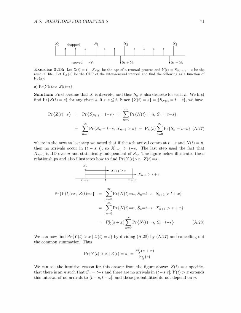
A.5. SOLUTIONS FOR CHAPTER 5 71
S0
6 6 6
?
6 6 6 6 6 6
?
dropped
served Y1 S1 + Y2 S2 + Y3
S1
?
S2 S3
Exercise 5.13: Let Z(t) = t � SN(t) be the age of a renewal process and Y (t) = SN(t)+1 � t be theresidual life. Let FX(x) be the CDF of the inter-renewal interval and find the following as a function ofFX(x):
a) Pr{Y (t)>x |Z(t)=s}
Solution: First assume that X is discrete, and thus Sn is also discrete for each n. We firstfind Pr{Z(t) = s} for any given s, 0 < s t. Since {Z(t) = s} = {SN(t) = t� s}, we have
Pr{Z(t)=s} = Pr�SN(t) = t�s
=
1Xn=0
Pr{N(t) = n, Sn = t�s}
=1X
n=0
Pr{Sn = t�s, Xn+1 > s} = FcX(s)
1Xn=0
Pr{Sn = t�s} (A.27)
where in the next to last step we noted that if the nth arrival comes at t� s and N(t) = n,then no arrivals occur in (t � s, t], so Xn+1 > t�s. The last step used the fact thatXn+1 is IID over n and statistically independent of Sn. The figure below illustrates theserelationships and also illustrates how to find Pr{Y (t)>x, Z(t)=s}.
tt� s t + x
Sn
6- Xn+1 > s + x
- Xn+1 > s
Pr{Y (t)>x, Z(t)=s} =1X
n=0
Pr{N(t)=n, Sn=t�s, Sn+1 > t + x}
=1X
n=0
Pr{N(t)=n, Sn=t�s, Xn+1 > s + x}
= FcX(s + x)
1Xn=0
Pr{N(t)=n, Sn=t�s} (A.28)
We can now find Pr{Y (t) > x | Z(t) = s} by dividing (A.28) by (A.27) and cancelling outthe common summation. Thus
Pr{Y (t) > x | Z(t) = s} =Fc
X(s + x)Fc
X(s)
We can see the intuitive reason for this answer from the figure above: Z(t) = s specifiesthat there is an n such that Sn = t�s and there are no arrivals in (t�s, t]; Y (t) > x extendsthis interval of no arrivals to (t� s, t + x], and these probabilities do not depend on n.

72 APPENDIX A. SOLUTIONS TO EXERCISES
The argument above assumed that X is discrete, but this is a technicality that could behandled by a limiting argument. In this case, however, it is cleaner to modify the aboveargument by working directly with the conditional probabilities.
Pr{Y (t) > x | Z(t) = s} =1X
n=0
Pr{N(t)=n}Pr�Y (t) > x | SN(t)=t�s, N(t)=n
=1X
n=0
Pr{N(t)=n}Pr{Xn+1 > t+s | Sn=t�s, Xn+1>s}
=F c
X(s+x)F c
X(s)
1Xn=0
Pr{N(t)=n} =F c
X(s+x)F c
X(s),
where the second line again uses the fact that {Sn=t�s, N(t)=n} = {Sn=t�s, Xn+1>s}.
b) Pr{Y (t)>x |Z(t+x/2)=s}.
Solution: The conditioning event {Z(t + x/2) = s} means that there is an arrival att+x/2� s and no further arrival until after t+x/2. We must look at two cases, first wherethe arrival at t + x/2 � s comes at or before t (i.e., s � x/2) and second where it comesafter t. The solution where s � x/2 is quite similar to (a), and we repeat the argumentthere for general X modifying the terms in (a) as needed. The diagram below will clarifythe various terms, assuming s � x/2.
tt + x2 � s t + x
2 t + x
Sn
6-Xn+1 > s
-Xn+1 > s + x2
As in (a),
PrnY (t)>x | Z(t+
x
2)=s
o=
1Xn=0
PrnN(t+
x
2)=n
oPrnY (t)>x | Z(t+
x
2)=s, N(t+
x
2)=n
o.
The conditioning event above isnZ�t +
x
2�
= s, N(t+x
2) = n
o=nSn = t +
x
2� s, Xn+1 > s
o. (A.29)
Given this conditioning event, the diagram shows that Y (t) > x implies that Xn+1 > s+x2 .
Thus
Prn
Y (t)>x | Z(t+x2)=s
o=
1Xn=0
Prn
N(t+x2)=n
oPrn
Xn+1>s+x2| Sn = t +
x2� s, Xn+1 > s
o
=Fc
X(s+x2 )
FcX(s)
for s � x/2. (A.30)
For the other case, where s < x/2, the condition asserts that SN(t+x2 ) > t. Thus there
must be an arrival in the interval from t to t+x2 , so Pr
�Y (t) > x | Z(t+x
2 )=s
= 0.
c) Pr{Y (t)>x |Z(t+x)>s} for a Poisson process.

A.5. SOLUTIONS FOR CHAPTER 5 73
Solution: The event {Z(t + x) > s} is the event that there are no arrivals in the interval(t+x�s, t+x]. We consider two cases separately, first s � x and next s < x. If s � x, thenthere are no arrivals from t to t + x, so that Y (t) must exceed x. Thus
Pr{Y (t) > x | Z(t + x) > s} = 1; for s � x.
Alternatively, if s < x, any arrival between t and t + x must arrive between t and t + x� s,so the probability of no arrival between t and t + x given no arrival between t + x� s andt + x is the probability of no arrival between t and t + x� s.
Pr{Y (t) > x | Z(t + x) > s} = exp�� �(x�s)
�; for s < x,
where � is the rate of the Poisson process.
Exercise 5.14: Let FZ(z) be the fraction of time (over the limiting interval (0,1)) that the age of arenewal process is at most z. Show that FZ(z) satisfies
FZ(z) =1
X
Z z
x=0
Pr{X > x} dx WP1.
Hint: Follow the argument in Example 5.4.7.
Solution: We want to find the time-average CDF of the age Z(t) of an arbitrary renewalprocess, and do this by following Example 5.4.7. For any given z > 0, define the rewardfunction R(t) to be 1 for Z(t) 1 and to be 0 otherwise, i.e.,
R(t) = R(Z(t), eX(t)) =
(1 ; Z(t) z0 ; otherwise .
Note that R(t) is positive only over the first z units of a renewal interval. Thus Rn =min(z,Xn). It follows that
E [Rn] = E [min(z,Xn)] =Z 1
0Pr{min(X, z) > x} dx (A.31)
=Z z
0Pr{X > x} dx. (A.32)
Let FZ(z) = limt!1R t0 (1/t)R(⌧) d⌧ denote the fraction of time that the age is less than or
equal to z. From Theorem 5.4.5 and (A.32),
FZ(z) =E [Rn]
X=
1X
Z z
0Pr{X > x} dx WP1.
Exercise 5.16: a) Use Wald’s equality to compute the expected number of trials of a Bernoulli process
up to and including the kth success.
Solution: In a Bernoulli process {Xn; n � 1, we call trial n a success if Xn = 1. Definea stopping trial J as the first trial n at which
Pnm=1 Xm = k. This constitutes a stopping
rule since IJ=n is a function of X1, . . . ,Xn. Given J = n, SJ = X1 + · · ·Xn = k, andsince this is true for all n, Sj = k unconditionally. Thus E [SJ ] = k. From Wald’s equality,E [SJ ] = XE [J ] so that E [J ] = k/X.

74 APPENDIX A. SOLUTIONS TO EXERCISES
We should have shown that E [J ] < 1 to justify the use of Wald’s equality, but we willshow that in (b).
b) Use elementary means to find the expected number of trials up to and including the first success. Use
this to find the expected number of trials up to and including the kth success. Compare with (a).
Solution: Let Pr{Xn = 1} = p. Then the first success comes at trial 1 with probability p,and at trial n with probability (1� p)n�1p. The expected time to the first success is then1/p = 1/X. The expected time to the kth success is then k/X, which agrees with the resultin (a).
The reader might question the value of Wald’s equality in this exercise, since the demon-stration that E [J ] < 1 was most easily accomplished by solving the entire problem byelementary means. In typical applications, however, the condition that E [J ] < 1 is essen-tially trivial.
Exercise 5.17: A gambler with an initial finite capital of d > 0 dollars starts to play a dollar slotmachine. At each play, either his dollar is lost or is returned with some additional number of dollars. LetXi be his change of capital on the ith play. Assume that {Xi; i=1, 2, . . . } is a set of IID random variablestaking on integer values {�1, 0, 1, . . . }. Assume that E [Xi] < 0. The gambler plays until losing all his money(i.e., the initial d dollars plus subsequent winnings).
a) Let J be the number of plays until the gambler loses all his money. Is the weak law of large numbers
su�cient to argue that limn!1 Pr{J > n} = 0 (i.e., that J is a random variable) or is the strong law
necessary?
Solution: We show below that the weak law is su�cient. The event {J > n} is the eventthat Si > �d for 1 i n. Thus Pr{J > n} Pr{Sn > �d}. Since E [Sn] = nX andX < 0, we see that the event {Sn > �d} for large n is an event in which Sn is very far aboveits mean. Putting this event in terms of distance from the sample average to the mean,
Pr{Sn > �d} = Pr⇢
Sn
n�X >
�d
n�X
�.
The WLLN says that limn!1 Pr�|Sn
n �X| > ✏
= 0 for all ✏ > 0, and this implies the samestatement with the absolute value signs removed, i.e., Pr
�Snn �X > ✏
= 0 for all ✏ > 0. If
we choose ✏ = �X/2 in the equation above, it becomes
limn!1
Pr⇢
Sn >nX
2
�= 0.
Since X < 0, we see that �d > nX/2 for n > 2��d/X
��, and thus limn!1 Pr{Sn > �d} = 0.
b) Find E [J ]. Hint: The fact that there is only one possible negative outcome is important here.
Solution: One stops playing on trial J = n if one’s capital reaches 0 for the first timeon the nth trial, i.e., if Sn = �d for the first time at trial n. This is clearly a functionof X1,X2, . . . ,Xn, so J is a stopping rule. Note that stopping occurs exactly on reaching�d since Sn can decrease with n only in increments of -1 and Sn is always integer. ThusSJ = �d

A.5. SOLUTIONS FOR CHAPTER 5 75
Using Wald’s equality, we then have
E [J ] =�d
X,
which is positive since X is negative. You should note from the exercises we have done withWald’s equality that it is often used to solve for E [J ] after determining E [SJ ].
For mathematical completeness, we should also verify that E [J ] < 1 to use Wald’s equality.If X is bounded, this can be done by using the Cherno↵ bound on Pr{Sn > �d}. Thisis exponentially decreasing in n, thus verifying that E [J ] < 1, and consequently thatE [J ] = �d/X. If X is not bounded, a truncation argument can be used. Letting Xb be X
truncated to b, we see that EhXb
iis increasing with b toward X, and is less E [X] for all b.
Thus the expected stopping time, say E [Jb] is upper bounded by �d/X for all b. It followsthat limb!1 E [Jb] is finite (and equal to �d/X). Most students are ill-advised to worry toomuch about such details at first.
Exercise 5.19: Let J = min{n |Snb or Sn�a}, where a is a positive integer, b is a negative integer,and Sn = X1 + X2 + · · ·+ Xn. Assume that {Xi; i�1} is a set of zero-mean IID rv’s that can take on onlythe set of values {�1, 0, +1}, each with positive probability.
a) Is J a stopping rule? Why or why not? Hint: The more di�cult part of this is to argue that J is a
random variable (i.e., non-defective); you do not need to construct a proof of this, but try to argue why it
must be true.
Solution: For J to be a stopping trial, it must be a random variable and also, for eachn, IJ=n must be a function of X1, . . . ,Xn. For the case here, Sn = X1+ · · ·+Xn isclearly a function of X1, . . . ,Xn, so the event that Sn � a or Sn b is a function ofX1, . . . ,Xn. The first n at which this occurs is a function of S1, . . . , Sn, which is a functionof X1, . . . ,Xn. Thus IJ=n must be a function of X1, . . . ,Xn. For J to be a rv, we mustshow that limn!1 Pr{J n} = 1. The central limit theorem states that (Sn � nX)/
pn�
approaches a normalized Gaussian rv in distribution as n ! 1. Since X is given to bezero-mean, Sn/
pn� must approach normal. Now both a/
pn� and b/
pn� approach 0 as
n !1, so the probability that {Sn; n > 0} (i.e., the process in the absence of a stoppingrule) remains between these limits goes to 0 as n ! 1. Thus the probability that theprocess has not stopped by time n goes to 0 as n !1.
An alternate approach here is to model {Sn;n � 1} for the stopped process as a Markovchain where a and b are recurrent states and the other states are transient. Then we knowthat one of the recurrent states are reached eventually with probability 1.
b) What are the possible values of SJ?
Solution: Since {Sn; n > 0} can change only in integer steps, Sn cannot exceed a withoutsome Sm, m < n first equaling a and it cannot be less than b without some Sk, k < n firstequaling b. Thus SJ is only a or b.
c) Find an expression for E [SJ ] in terms of p, a, and b, where p = Pr{SJ � a}.
Solution: E [SJ ] = aPr{SJ = a}+ bPr{SJ = b} = pa + (1� p)b
d) Find an expression for E [SJ ] from Wald’s equality. Use this to solve for p.

76 APPENDIX A. SOLUTIONS TO EXERCISES
Solution: We have seen that J is a stopping trial for the IID rv’s {Xi; i > 0}. Assumingfor the moment that E [J ] < 1, Wald’s equality holds and E [SJ ] = XE [J ]. Since X = 0,we conclude that E [SJ ] = 0. Combining this with (c), we have 0 = pa + (1 � p)b, sop = �b/(a� b). This is easier to interpret as
p = |b|/(a + |b|). (A.33)
The assumption that E [J ] < 1 is more than idle mathematical nitpicking, since we sawin Example 5.5.4 that E [J ] = 1 for b = �1. The CLT does not resolve this issue, sincethe probability that Sn is outside the limits [�b, a] approaches 0 with increasing n only asn�1. Viewing the process as a finite-state Markov chain with a and b viewed as a commontrapping state does resolve the issue, since, as seen in Theorem 4.5.4 applied to expectedfirst passage times, the expected time to reach the trapping state is finite. As will be seenwhen we study Markov chains with countably many states, this result is no longer valid,as illustrated by Example 5.5.4. This issue will become more transparent when we studyrandom walks in Chapter 9.
The solution in (A.33) applies only for X = 0, but Chapter 9 shows how to solve the problemfor an arbitrary distribution on X. We also note that the solution is independent of pX(0),although pX(0) is obviously involved in finding E [J ]. Finally we note that this helps explainthe peculiar behavior of the ‘stop when you’re ahead’ example. The negative threshold brepresents the capital of the gambler in that example and shows that as b ! �1, theprobability of reaching the threshold a increases, but at the expense of a larger catastopheif the gamblers capital is wiped out.
Exercise 5.31: Customers arrive at a bus stop according to a Poisson process of rate �. Independently,buses arrive according to a renewal process with the inter-renewal interval CDF FX(x). At the epoch of abus arrival, all waiting passengers enter the bus and the bus leaves immediately. Let R(t) be the number ofcustomers waiting at time t.
a) Draw a sketch of a sample function of R(t).
Solution: Let Sn = X1 +X2 + · · · be the epoch of the nth bus arrival and Cm the epoch ofthe mth customer arrival. Then {Cm;m � 1} is the sequence of arrival times in a Poissonprocess of rate � and {Sn;n � 1} is the renewal time sequence of a renewal process.
C1 C2 C3S1
C4 C5S2
C6 t
R(t)
b) Given that the first bus arrives at time X1 = x, find the expected number of customers picked up; then
find E⇥R x
0R(t)dt
⇤, again given the first bus arrival at X1 = x.
Solution: The expected number of customers picked up, given S1 = x is the expectednumber of arrivals in the Poisson process by x, i.e., �x. For t < x, R(t) is the number ofcustomers that have arrived by time t. R(t), for t < S1, is independent of S1, so
E
Z x
0R(t) dt
�=Z x
0�xdx =
�x2
2.

A.5. SOLUTIONS FOR CHAPTER 5 77
c) Find limt!11t
R t
0R(⌧)d⌧ (with probability 1). Assuming that FX is a non-arithmetic distribution, find
limt!1 E [R(t)]. Interpret what these quantities mean.
Solution: In (b), we found the expected reward in an inter-renewal interval of size x, i.e.,we took the expected value over the Poisson process given a specific value of X1. Takingthe expected value of this over the bus renewal interval, we get (1/2)�E
⇥X2⇤. This is
the expected accumulated reward over the first bus inter-renewal period, denoted E [R1] in(5.22). It is the expected number of customers at each time, integrated over the time untilthe first bus arrival. This integrated value is not the expected number waiting for a bus,but rather will be used as a step in finding the time-average number waiting over time.Since the bus arrivals form a renewal process, this is equal to E [Rn] for each inter-renewalperiod n. By (5.24),
limt!1
1t
Z t
0R(⌧)d⌧ =
E [Rn]X
=�E⇥X2⇤
2XWP1. (A.34)
Since the renewals are non-arithmetic, this is the same as limt!1 E [R(t)].
Note that this is not the same as the expected number of customers per bus. It is theexpected number of waiting customers, averaged over time. If a bus is highly delayed, alarge number of customers accumulate, but also, because of the large interval waiting forthe bus, the contribution to the time average grows as the square of the wait.
d) Use (c) to find the time-average expected wait per customer.
Solution: Little’s theorem can be applied here since (A.34) gives the limiting time-average number ofcustomers in the system, L. The time-average wait per customer W is W = L/�, which from (A.34) isE⇥X2⇤/2X. The system here does not satisfy the conditions of Little’s theorem, but it is easy to check that
the proof of the theorem applies in this case.
e) Find the fraction of time that there are no customers at the bus stop. (Hint: this part is independent of
(a), (b), and (c); check your answer for E [X] << 1/�).
Solution: There are no customers at the bus stop at the beginning of each renewal period.Let Un be the interval from the beginning of the nth renewal period until the first customerarrival. It is possible that no customer will arrive before the next bus arrives, so the intervalwithin the nth inter-renewal period when there is no customer waiting is min(Un,Xn).Consider a reward function R(t) equal to 1 when no customer is in the system and 0otherwise. The accumulated reward Rn within the nth inter-renewal period is then Rn =min(Un,Xn). Thus, using the independence of Un and Xn,
E [Rn] =Z 1
0Pr{min(Un,Xn) > t} dt =
Z 1
0Pr{(Un > t}Pr{Xn > t} dt
=Z t
0Pr{Xn > t} e��t dt.
Using (5.24), the limiting time-average fraction of time when no customers are waiting is(1/X)
R t0 Pr{Xn > t} e��t dt. Checking when X << 1/�, we see that the above integral is
close to X. In particular, if Xn is exponential with rate µ, we see that the fraction aboveis µ/(µ + �).

78 APPENDIX A. SOLUTIONS TO EXERCISES
Exercise 5.44: This is a very simple exercise designed to clarify confusion about the roles of past,present, and future in stopping rules. Let {Xn; n � 1} be a sequence of IID binary rv’s , each with the pmfpX(1) = 1/2, pX(0) = 1/2. Let J be a positive integer-valued rv that takes on the sample value n of thefirst trial for which Xn = 1. That is, for each n � 1,
{J = n} = {X1=0, X2=0, . . . , Xn�1=0, Xn=1}.
a) Use the definition of stopping trial, Definition 5.5.1, to show that J is a stopping trial for {Xn; n � 1}.
Solution: Note that IJ=n = 1 if Xn = 1 and Xi = 0 for all i < n. IJ=n = 0 otherwise.Thus IJ=n is a function of X1, . . . ,Xn. We also see that J is a positive integer-valued rv.That is, each sample sequence of {Xi; i � 1} (except the zero probability sequence of allzeros) maps into a positive integer.
b) Show that for any given n, the rv’s Xn and IJ=n are statistically dependent.
Solution: Note that Pr{IJ=n = 1} = 2�n and Pr{Xn = 1} = 1/2. The product of these is2�(n+1), whereas Pr{Xn = 1, IJ=n = 1} = 2�n, demonstrating statistical dependence. Moreintuitively Pr{Xn = 1 | IJ=n = 1} = 1 and Pr{Xn = 1} = 1/2.
c) Show that for every m > n, Xn and IJ=m are statistically dependent.
Solution: For m > n, IJ=m=1 implies that Xi = 0 for i < m, and thus that Xn = 0. ThusPr{Xn = 1 | IJ=m=1} = 0. Since Pr{Xn = 1} = 1/2, IJ=m and Xn are dependent.
d) Show that for every m < n, Xn and IJ=m are statistically independent.
Solution: Since IJ=m is a function of X1, . . . ,Xm and Xn is independent of X1, . . . ,Xm,it is clear that Xn is independent of IJ=m
e) Show that Xn and IJ�n are statistically independent. Give the simplest characterization you can of the
event {J � n}.
Solution: For the same reason as IJ=m is independent of Xn for m < n, we see that IJ<n
is independent of Xn. Now {J � n} = {J < n}c, so IJ�n = 1� IJ<n. Thus {J � n} is alsoindependent of Xn. We give an intuitive explanation after (f).
f) Show that Xn and IJ>n are statistically dependent.
Solution: The event {J > n} implies that X1, . . . ,Xn are all 0, so Pr{Xn = 1 | J > n} = 0.Since Pr{Xn=1} = 1/2, it follows that Xn and IJ>n are dependent.
It is important (and essentially the central issue of the exercise) to understand why (e) and(f) are di↵erent. Note that {J � n} = {J = n}
S{J > n}. Now {J = n} implies that
Xn = 1 whereas {J > n} implies that Xn = 0. The union, however, implies nothing aboutXn, and is independent of Xn. The union, IJ�n is the event that X1, . . . ,Xn�1 are all 0and Xn then determines whether J = n or J > n.
Note: The results here are characteristic of most sequences of IID rv’s. For most people, this requires some
realignment of intuition, since {J�n} is the union of {J=m} for all m � n, and each of these events are
highly dependent on Xn. The right way to think of this is that {J�n} is the complement of {J<n}, which
is determined by X1, . . . , Xn�1. Thus {J�n} is also determined by X1, . . . , Xn�1 and is thus independent
of Xn. The moral of the story is that thinking of stopping rules as rv’s independent of the future is very
tricky, even in totally obvious cases such as this.

A.6. SOLUTIONS FOR CHAPTER 6 79
A.6 Solutions for Chapter 6
Exercise 6.1: Let {Pij ; i, j � 0} be the set of transition probabilities for a countable-state Markov
chain. For each i, j, let Fij(n) be the probability that state j occurs sometime between time 1 and n
inclusive, given X0 = i. For some given j, assume that {xi; i � 0} is a set of nonnegative numbers satisfying
xi = Pij +P
k 6=j Pikxk for all i � 0. Show that xi � Fij(n) for all n and i, and hence that xi � Fij(1) for
all i. Hint: use induction.
Solution: We use induction on n. As the basis for the induction, we know that Fij(1) = Pij .Since the xi are by assumption nonnegative, it follows for all i that
Fij(1) = Pij Pij +Xk 6=j
Pikxk = xi.
For the inductive step, assume that Fij(n) xi for a given n and all i. Using (6.8),
Fij(n + 1) = Pij +Xk 6=j
PikFkj(n)
Pij +Xk 6=j
Pikxk = xi for all i.
By induction, it then follows that Fij(n) xi for all i, n. From (6.7), Fij(n) is non-decreasing in n and upper bounded by 1. It thus has a limit, Fij(1), which satisfiesFij(1) xi for all i.
One solution to the set of equations xi = Pij +P
k 6=j Pikxk is xi = 1 for all i. Another (from6.9)) is xi = Fij(1). These solutions are di↵erent when Fij(1) < 1, and this exercise thenshows that the solution {Fij(1); i � 0} is the smallest of all possible solutions.
Exercise 6.2: a) For the Markov chain in Figure 6.2, show that, for p � 1/2, F00(1) = 2(1 � p) and
show that Fi0(1) = [(1� p)/p]i for i � 1. Hint: first show that this solution satisfies (6.9) and then show
that (6.9) has no smaller solution (Exercise 6.1 shows that Fij(1) is the smallest solution to (6.9)). Note
that you have shown that the chain is transient for p > 1/2 and that it is recurrent for p = 1/2.
Solution: Note that the diagram in Figure 6.2 implicitly assumes p < 1, and we assumethat here, since the p = 1 case is trivial anyway.
The hint provides a straightforward algebraic solution, but provides little insight. It maybe helpful, before carrying that solution out, to solve the problem by the more intuitivemethod used in the ‘stop when you’re ahead’ example, Example 5,4.4. This method alsoderives the values of Fi0(1) rather than just verifying that they form a solution.
Let F10(1) be denoted by ↵. This is the probability of ever reaching state 0 starting fromstate 1. This probability is unchanged by converting state 0 to a trapping state, since whenstarting in state 1, transitions from state 0 can occur only after reaching state 0.
In the same way, Fi,i�1(1) for any i > 1 is unchanged by converting state i�1 into atrapping state, and the modified Markov chain, for states k � i�1 is then the same as themodified chain that uses state 0 as a trapping state. Thus Fi,i�1(1) = ↵.

80 APPENDIX A. SOLUTIONS TO EXERCISES
We can proceed from this to calculate Fi,i�2 for any i > 2. In order to access state i � 2from state i, it is necessary to first access state i� 1. Given a first passage from i to i� 1,(an event of probability ↵), it is necessary to have a subsequent first passage from i� 1 toi� 2, so Fi,i�2(1) = ↵2. Iterating on this, Fi0(1) = ↵i.
We can now solve for ↵ by using (6.9) for i = 1, j = 0: F10(1) = q + pF20(1). Thus↵ = q + p↵2. This is a quadratic equation in ↵ with the solutions ↵ = 1 and ↵ = q/p. Wethen know that F10(1) has either the value 1 or q/p. For whichever value of ↵ is correct,we also have Pi0(1) = ↵i for i � 1. Finally, from (6.9) for j = 0, i = 0, F00(1) = q + p↵.
From the reasoning above, we know that these two possible solutions are the only possi-bilities. If both of them satisfy (6.9), then, from Exercise 6.1, the one with ↵ = q/p isthe correct one since it is the smaller solution to (6.9). We now show that the solutionwith ↵ = q/p satisfies (6.9). This is the first part of what the question asks, but it is nowunnecessary to also show that this is the smallest solution.
If we substitute the hypothesized solution,
F00(1) = 2q; Fi0(1) = (q/p)i for i > 0, (A.35)
into (6.9) for j = 0, we get the hypothesized set of equalities,
2q = q + p(q/p) for i = 0q/p = q + p(q/p)2 for i = 1
(q/p)i = q(q/p)i�1 + p(q/p)i+1 for all i � 2.
The first of these is clearly an identity, and the third is seen to be an identity by rewritingthe right side as p(q/p)i + q(q/p)i. The second is an identity by almost the same argument.Thus (A.35) satisfies (6.9) and thus gives the correct solution.
For those who dutifully took the hint directly, it is still necessary to show that (A.35) is thesmallest solution to (6.9). Let xi abbreviate Fi0(1) for i � 0. Then (6.9) for j = 0 can berewritten as
x0 = q + px1
x1 = q + px2
xi = qxi�1 + pxi+1 for i � 2.
The equation for each i � 2 can be rearranged to the alternate form,
xi+1 � (q/p)xi = xi � (q/p)xi�1. (A.36)
For i = 1, the similar rearrangement is x2�(q/p)x1 = x1�q/p. Now consider the possibilityof a solution to these equations with x1 < q/p, say x1 = (q/p) � � with � > 0. Recursingon the equations (A.36), we have
xi+1 � (q/p)xi = �� for i � 1. (A.37)
For the case q = p = 1/2, this becomes xi+1 � xi = ��. Thus for su�ciently large i, xi
becomes negative, so there can be no non-negative solution of (6.9) with F10 < q/p.
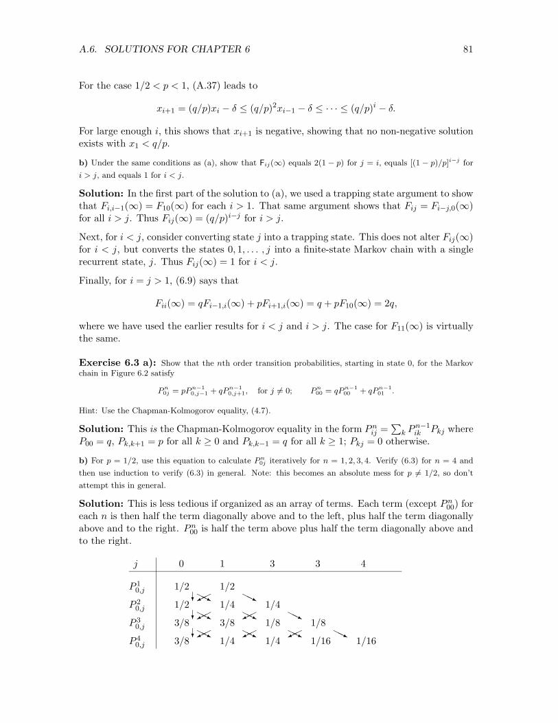
A.6. SOLUTIONS FOR CHAPTER 6 81
For the case 1/2 < p < 1, (A.37) leads to
xi+1 = (q/p)xi � � (q/p)2xi�1 � � · · · (q/p)i � �.
For large enough i, this shows that xi+1 is negative, showing that no non-negative solutionexists with x1 < q/p.
b) Under the same conditions as (a), show that Fij(1) equals 2(1 � p) for j = i, equals [(1 � p)/p]i�j for
i > j, and equals 1 for i < j.
Solution: In the first part of the solution to (a), we used a trapping state argument to showthat Fi,i�1(1) = F10(1) for each i > 1. That same argument shows that Fij = Fi�j,0(1)for all i > j. Thus Fij(1) = (q/p)i�j for i > j.
Next, for i < j, consider converting state j into a trapping state. This does not alter Fij(1)for i < j, but converts the states 0, 1, . . . , j into a finite-state Markov chain with a singlerecurrent state, j. Thus Fij(1) = 1 for i < j.
Finally, for i = j > 1, (6.9) says that
Fii(1) = qFi�1,i(1) + pFi+1,i(1) = q + pF10(1) = 2q,
where we have used the earlier results for i < j and i > j. The case for F11(1) is virtuallythe same.
Exercise 6.3 a): Show that the nth order transition probabilities, starting in state 0, for the Markovchain in Figure 6.2 satisfy
P n0j = pPn�1
0,j�1 + qP n�10,j+1, for j 6= 0; P n
00 = qP n�100 + qP n�1
01 .
Hint: Use the Chapman-Kolmogorov equality, (4.7).
Solution: This is the Chapman-Kolmogorov equality in the form Pnij =
Pk Pn�1
ik Pkj whereP00 = q, Pk,k+1 = p for all k � 0 and Pk,k�1 = q for all k � 1; Pkj = 0 otherwise.
b) For p = 1/2, use this equation to calculate P n0j iteratively for n = 1, 2, 3, 4. Verify (6.3) for n = 4 and
then use induction to verify (6.3) in general. Note: this becomes an absolute mess for p 6= 1/2, so don’t
attempt this in general.
Solution: This is less tedious if organized as an array of terms. Each term (except Pn00) for
each n is then half the term diagonally above and to the left, plus half the term diagonallyabove and to the right. Pn
00 is half the term above plus half the term diagonally above andto the right.
j 0 1 3 3 4
P 10,j 1/2 1/2
HHj
HHj
HHj
��⇡
��⇡
��⇡
?
?
?
HHj
HHj
HHj
HHj
HHj HHj
��⇡
��⇡ ��⇡
P 20,j 1/2 1/4 1/4
P 30,j 3/8 3/8 1/8 1/8
P 40,j 3/8 1/4 1/4 1/16 1/16

82 APPENDIX A. SOLUTIONS TO EXERCISES
terms are similar. We also see (with less work) that (6.3) is valid for 1 n 3 for allj, 0 j n. We can avoid fussing with the constraint j n by following the conventionthat
�nk
�= 0 for all n � 1 and k > n. We have then shown that (6.3) is valid for 1 n 4
and all j � 0.
We next use induction to validate (6.3) in general. From the previous calculation, anyn, 1 n 4 can be used as the basis of the induction and then, given the assumption that(6.3) is valid for any given n > 0 and all j � 0, we will prove that (6.3) is also valid forn+1 and all j � 0. Initially, for given n, we assume j > 0; the case j = 0 is a little di↵erentsince it has self transitions, so we consider it later.
For the subcase where n + j is even, we have
Pn+10j =
12⇥Pn
0,j�1 + Pn0,j+1
⇤
=12
✓n
(j + n)/2
◆2�n +
✓n
((j + n)/2) + 1
◆2�n
�
=✓
n + 1((j + n)/2) + 1
◆2�(n+1).
The first equality comes from part (a) with p = q = 1/2. The second equality uses (6.3) forthe given n and uses the fact that n+j�1 and n+j+1 are odd. The final equality followsimmediately from the combinatorial identity
✓n
k
◆+✓
n
k + 1
◆=✓
n + 1k + 1
◆.
This identity follows by viewing�n+1k+1
�as the number of ways to arrange k + 1 ones in a
binary n + 1 tuple. These arrangements can be separated into those that start with a onefollowed by k ones out of n and those that start with a zero followed by k + 1 ones out ofn. The final result for Pn+1
0j above is for n+1+j odd and agrees with the odd case in (6.3)after substituting n+1 for n in (6.3). This validates (6.3) for this case. The subcase wheren+j is odd is handled in the same way.
For the case j = 0, we use the second portion of part (a), namely Pn+100 = 1
2Pn00 + 1
2Pn01. For
the subcase where n is even, we then have
Pn+100 =
12
✓n
n/2
◆2�n +
✓n
(n/2) + 1
◆2�n
�
=✓
n+1(n/2)+1
◆2�(n+1).
In the first equality, we have used (6.3) with n+j even for j=0 and n+j odd for j=1. Thesecond equality uses the combinatorial identity above. This result agrees with the odd casein (6.3) after substituting n+1 for n. Finally, the subcase where n is odd is handled inalmost the same way, except that one must recognize that
� n(n+1)/2
�=� n(n�1)/2
�.
(c) As a more interesting approach, which brings out the relationship of Figures 6.2 and 6.1, note that (6.3),
with j + n even, is the probability that Sn = j for the chain in 6.1. Similarly, (6.3) with j + n odd is the

A.6. SOLUTIONS FOR CHAPTER 6 83
probability that Sn = �j� 1 for the chain in 6.1. By viewing each transition over the self loop at state 0 as
a sign reversal for the chain in 6.1, explain why this surprising result is true. (Again, this doesn’t work for
p 6= 1/2, since the sign reversals also reverse the +1, -1 transitions.)
Solution: The meaning of the hint will be less obscure if we redraw Figure 6.1 in thefollowing way:
�1 �2 �3
n1/2 1/2
1/2 1/2
1/2 1/2
1/2 1/2
. . .n XzXy
n XzXy0 1 2
n
even
even
even
odd
odd
odd
�
↵
1/21/2
. . .n XzXy
n XzXy
Figure 6.1 redrawn
Compare this with the discrete M/M/1 chain of Figure 6.2,
0 1 2n1/2 1/2
1/2 1/2 1/2. . .⇠: n Xz
Xyn XzXy Figure 6.2 redrawn
Note that Figure 6.2 can be viewed as the result of combining each nonnegative state i inthe redrawn Figure 6.1 with the state �i�1 lying directly beneath it. To be more specific,the transition probability from state 0 in Fig. 6.1 to the aggregated states 1 and -2 is 1/2,and the transition probability to the aggregated states 0 and -1 is 1/2. The same transitionprobabilities hold for state -1. Similarly, starting from any state i in Fig 6.1, there is atransition probablity 1/2 to the aggregated states i+1,�i�2 and 1/2 to the aggregatedstates i � 1 and i. The same aggregated transition probabilities hold starting from state�i�1.
What this means is that the set of aggregated pairs forms a Markov chain in its own right,and this Markov chain is the M/M/1 chain of Fig 6.2. The nth order transition probabilitesPn
0i for the M/M/1 chain are thus the same as the nth order aggregate transition probabilitiessay Qn
0i + Qn0,�i�1 for the Bernoulli chain. Since the Bernoulli chain is periodic with period
2, however, and each pair of states consists of one even and one odd term, only one of theseaggregated terms is nonzero. This helps explain the strange looking di↵erence in part (b)between n + i even and odd.
Exercise 6.8: Let {Xn; n � 0} be a branching process with X0 = 1. Let Y , �2 be the mean and varianceof the number of o↵spring of an individual.
a) Argue that limn!1Xn exists with probability 1 and either has the value 0 (with probability F10(1)) or
the value 1 (with probability 1� F10(1)).
Solution: We consider 2 special, rather trivial, cases before considering the importantcase (the case covered in the text). Let pi be the PMF of the number of o↵spring of eachindividual. Then if p1 = 1, we see that Xn = 1 for all n, so the statement to be argued issimply false. You should be proud of yourself if you noticed the need for ruling this caseout before constructing a proof.
The next special case is where p0 = 0 and p1 < 1. Then Xn+1 � Xn (i.e., the populationnever shrinks but can grow). Since Xn(!) is non-decreasing for each sample path, either

84 APPENDIX A. SOLUTIONS TO EXERCISES
limn!1Xn(!) = 1 or limn!1Xn(!) = j for some j < 1. The latter case is impossible,since Pjj = pj
1 and thus Pmjj = pmj
1 ! 0 as m !1.
Ruling out these two trivial cases, we have p0 > 0 and p1 < 1 � p0. In this case, state 0is recurrent (i.e., it is a trapping state) and states 1, 2, . . . are in a transient class. To seethis, note that P10 = p0 > 0, so F11(1) 1� p0 < 1, which means by definition that state1 is transient. All states i > 1 communicate with state 1, so by Theorem 6.2.5, all statesj � 1 are transient. Thus one can argue that the process has ‘no place to go’ other than 0or 1.
The following tedious analysis makes this precise. Each j > 0 is transient, so from Theorem6.2.6 part 3,
limt!1
E [Njj(t)] < 1.
Note that N1j(t) is the number of visits to j in the interval [1, t] starting from state 1 attime 0. This is one more than the number of returns to j after the first visit to j. Theexpected number of such returns is upper bounded by the number in t steps starting in j,so E [N1j(t)] 1 + E [Njj(t)]. It follows that
limt!1
E [N1j(t)] < 1 for each j > 0.
Now note that the expected number of visits to j in [1, t] can be rewritten asPt
n=1 Pij(n).Since this sum in the limit t ! 1 is finite, the remainder in the sum from t to 1 mustapproach 0 as t !1, so
limt!1
Xn>t
Pn1j = 0.
From this, we see that for every finite integer `,
limt!1
Xn>t
Xj=1
Pn1j = 0.
This says that for every ✏ > 0, there is a t su�ciently large that the probability of everentering states 1 to ` on or after step t is less than ✏. Since ✏ > 0 is arbitrary, all samplepaths (other than a set of probability 0) never enter states 1 to ` after some finite time.Since ` is arbitrary, limn!1Xn exists WP1 and is either 0 or 1. By definition, it is 0 withprobability F10(1).
b) Show that VAR [Xn] = �2Yn�1
(Yn � 1)/(Y � 1) for Y 6= 1 and VAR [Xn] = n�2 for Y = 1.
Solution: We will demonstrate the case for Y 6= 1 and Y = 1 together by showing that
VAR [Xn] = �2Yn�1h1 + Y + Y
2 + · · ·+ Yn�1i. (A.38)
A.6. SOLUTIONS FOR CHAPTER 6 85
First express E⇥X2
n
⇤in terms of E
⇥X2
n�1
⇤. Note that, conditional on Xn�1 = `, Xn is the
sum of ` IID rv’s each with mean Y and variance �2, so
E⇥X2
n
⇤=
X`
Pr{Xn�1 = `}E⇥X2
n | Xn�1 = `⇤
=X
`
Pr{Xn�1 = `}h`�2 + `2Y
2i
= �2E [Xn�1] + Y2E⇥X2
n�1
⇤= �2Y
n�1 + Y2E⇥X2
n�1
⇤.
We also know from (6.50) (or by simple calculation) that E [Xn] = Y E [Xn�1]. Thus,
VAR [Xn] = E⇥X2
n
⇤�hE [Xn]
i2= �2Y
n�1 + Y2VAR [Xn�1] . (A.39)
We now use induction to derive (A.38) from (A.39). For the base of the induction, we seethat X1 is the number of progeny from the single element X0, so VAR [X1] = �2. For theinductive step, we assume that
VAR [Xn�1] = �2Yn�2h1 + Y + Y
2 + · · ·+ Yn�2i.
Substituting this into (A.39),
VAR [Xn] = �2Yn�1 + �2Y
nh1 + Y + · · ·+ Y
n�2i
= �2Yn�1h1 + Y + · · ·+ Y
n�1i,
completing the induction.
Exercise 6.9: There are n states and for each pair of states i and j, a positive number dij = dji is given.A particle moves from state to state in the following manner: Given that the particle is in any state i, itwill next move to any j 6= i with probability Pij given by
Pij =dijP
k 6=i dik. (A.40)
Assume that Pii = 0 for all i. Show that the sequence of positions is a reversible Markov chain and find the
limiting probabilities.
Solution: From Theorem 6.5.3, {Pij} is the set of transition probabilities and ⇡⇡⇡ is thesteady state probability vector of a reversible chain if ⇡iPij = ⇡jPji for all i, j. Thus, given{dij}, we attempt to find ⇡⇡⇡ to satisfy the equations
⇡iPij =⇡idijP
k dik=
⇡jdjiPk djk
= ⇡jPji; for all i, j.
We have taken dii = 0 for all i here. Since dij = dji for all i, j, we can cancel dij and dji
from the inner equations, getting
⇡iPk dik
=⇡jPk djk
; for all i, j.

86 APPENDIX A. SOLUTIONS TO EXERCISES
Thus ⇡i must be proportional toP
k dik, so normalizing to makeP
i ⇡i = 1, we get
⇡i =P
k dikP`
Pk d`k
; for all i.
If the chain has a countably infinite number of states, this still works if the sums exist.
This exercise is not quite as specialized as it sounds, since given any reversible Markov chain,we can definite dij = ⇡iPij and get this same set of equations (normalized in a special way).
Exercise 6.10: Consider a reversible Markov chain with transition probabilities Pij and limiting prob-abilities ⇡i. Also consider the same chain truncated to the states 0, 1, . . . , M . That is, the transitionprobabilities {P 0ij} of the truncated chain are
P 0ij =
(PijPm
k=0 Pik; 0 i, j M
0 ; elsewhere..
Show that the truncated chain is also reversible and has limiting probabilities given by
⇡i =⇡iPM
j=0 PijPMk=0
⇣⇡k
PMm=0 Pkm
⌘ . (A.41)
Solution: The steady state probabilities {⇡i; i � 0} of the original chain must be positive.Thus ⇡i > 0 for each i. By summing ⇡i over i in (A.41), it is seen that the numerator isthe same as the denominator, so
PMi=0 ⇡i = 1. Finally,
⇡iP0ij =
⇡iPijPMk=0
⇣⇡kPM
m=0 Pkm
⌘ .
Since ⇡iPij = ⇡jPji for each i, j, it is clear that ⇡iP 0ij = ⇡jP 0
ji for each i, j M. Thus,by Theorem 6.5.3, the truncated chain is reversible. It seems like this should be obviousintuititvely, but the rules for truncation are su�ciently complicated that it doesn’t seemobvious at all.
Exercise 6.12: a) Use the birth and death model described in figure 6.4 to find the steady-stateprobability mass function for the number of customers in the system (queue plus service facility) for thefollowing queues:
i) M/M/1 with arrival probability ��, service completion probability µ�.
ii) M/M/m with arrival probability ��, service completion probability iµ� for i servers busy, 1 i m.
iii) M/M/1 with arrival probability ��, service probability iµ� for i servers. Assume � so small that iµ� < 1for all i of interest.
Assume the system is positive recurrent.
Solution: M/M/1: This is worked out in detail in section 6.6. From (6.45), ⇡i = (1�⇢)⇢i
where ⇢ = �/µ < 1.
M/M/m: The Markov chain for this is

A.6. SOLUTIONS FOR CHAPTER 6 87
0 1 2 m m+1Xz
�. . . nn�� �� �� ��
µ� 2µ� mµ� mµ�
. . .O O O O
⇠: n XzXy
n XzXy
n XzXy
This is a birth-death chain and the steady state probabilitiers are given by (6.33) where⇢i = �/((i+1)µ) for i < m and ⇢i = �/mµ for i � m. Evaluating this,
⇡i =⇡0(�/µ)i
i!for i < m; ⇡i =
⇡0(�/µ)i
m!(mi�m)for i � m,
where ⇡0 is given by
⇡�10 = 1 +
m�1Xi=1
(�/µ)i
i!+
(m⇢m)m
m!(1� ⇢m). (A.42)
M/M/1: The assumption that � is so small that iµ� < 1 for all ‘i of interest’ is ratherstrange, since we don’t know what is of interest. When we look at the solution to theM/M/1 and M/M/m sample-time queues above, however, we see that they do not dependon �. It is necessary for mµ� 1 for the Markov chain to be defined, and mµ� << 1 forit to be a reasonable approximation to the behavior of the continuous time queue, but theresults turn out to be the same as the continuous time queue in any case, as will be seen inChapter 7. What was intended here was to look at the limit of the M/M/m queue in thelimit m !1. When we do this,
⇡i =⇡0(�/µ)i
i!for all i,
where
⇡�10 = 1 +
1Xi=1
(�/µ)i
i!.
Recognizing this as the power series of an exponential, ⇡0 = e��/µ.
b) For each of the queues above give necessary conditions (if any) for the states in the chain to be i) transient,
ii) null recurrent, iii) positive recurrent.
Solution: The M/M/1 queue is transient if �/µ > 1, null recurrent if �/µ = 1, and positiverecurrent if �/µ < 1 (see Section 6.6). In the same way, the M/M/m queue is transient if�/mµ > 1, null recurrent if �/mµ = 1 and positive recurrent if �/mµ < 1. The M/M/1queue is positive recurrent in all cases. As the arrival rate speeds up, the number of serversin use increases accordingly.
c) For each of the queues find:
L = (steady-state) mean number of customers in the system.
Lq = (steady-state) mean number of customers in the queue.
W = (steady-state) mean waiting time in the system.
W q = (steady-state) mean waiting time in the queue.

88 APPENDIX A. SOLUTIONS TO EXERCISES
Solution: The above parameters are related in a common way for the three types of queues.First, applying Little’s law first to the system and then to the queue, we get
W = L/�; W q = Lq/�. (A.43)
Next, define Lv as the steady-state mean number of customers in service and W v as thesteady state waiting time per customer in service. We see that for each system, W v = 1/µ,since when a customer enters service the mean time to completion is 1/µ. From Little’s lawapplied to service, Lv = �/µ. Now L = Lq + Lv and W = W q + W v. Thus
L = Lq + �/µ; W = W q + 1/µ. (A.44)
Thus for each of the above queue types, we need only compute one of these four quantitiesand the others are trivially determined. We assume positive recurrence in all cases.
For M/M/1, we compute
L =X
i
i⇡i = (1� ⇢)1Xi=0
i⇢i =⇢
1� ⇢=
�
µ� �.
For M/M/m, we compute Lq since queueing occurs only in states i > m.
Lq =Xi>m
(i�m)⇡i =Xi>m
(i�m)⇡0(�/µ)i
m!(mi�m)
=Xj>0
j⇡0⇢jm(�/µ)m
m!=
⇡0⇢m(�/µ)m
(1� ⇢m)2m!,
where ⇡0 is given in (A.42).
Finally, for M/M/1, there is no queueing, so Lq = 0.
Exercise 6.14: Find the backward transition probabilities for the Markov chain model of age in Figure
6.3. Draw the graph for the backward Markov chain, and interpret it as a model for residual life.
Solution: The backward transition probabilities are by definition given by P ⇤ij = ⇡jPji/⇡i.
Since the steady state probabilities ⇡i are all positive, P ⇤ij > 0 if and only if Pji > 0. Thus
the graph for the backward chain is the same as the forward chain except that all the arrowsare reversed, and, of course, the labels are changed accordingly. The graph shows that thereis only one transition coming out of each positive numbered state in the backward chain.Thus P ⇤
i,i�1 = 1 for all i > 0. This can be easily verified algebraically from 6.27. It is alsoseen that P ⇤
i0 = Pr{W = i + 1}.
0 1 2 3 4P ⇤00 P ⇤10 P ⇤21 P ⇤32 P ⇤43
P ⇤01 P ⇤02 P ⇤03 P ⇤04
⇣1 ⇣1 ⇣1. . .
⇠:n⇠9n⇠9 n⇠9 n⇠9
⇠: n
We can interpret this Markov chain as representing residual life for an integer renewalprocess. The number of the state represents the residual life immediately before a transition,

A.6. SOLUTIONS FOR CHAPTER 6 89
i.e., state 0 means that a renewal will happen immediately, state 1 means that it will happenin one time unit, etc. When a renewal occurs, the next state will indicate the residual life atthe end of that unit interval. Thus when a transition from 0 to i occurs, the correspondingrenewal interval is i + 1.
For those confused by both comparing the chain above as the backward chain of age inFigure 6.3 and as the residual life chain of the same renewal process, consider a samplepath for the renewal process in which an inter-renewal interval of 5 is followed by one of 2.The sample path for age in Figure 6.3 is then (0, 1, 2, 3, 4, 0, 1, 2, 0) The sample path forresidual life for the same sample path of inter-renewals, for the interpretation above, is (0,4, 3, 2, 1, 0, 2, 1, 0). On the other hand, the backward sample path for age is (0, 2, 1, 0,4, 3, 2, 1, 0). In other words, the residual life sample path runs backward from age withineach renewal interval, but forward between renewals.

90 APPENDIX A. SOLUTIONS TO EXERCISES
A.7 Solutions for Chapter 7
Exercise 7.1: Consider an M/M/1 queue as represented in Figure 7.4. Assume throughout that X0 = iwhere i > 0. The purpose of this exercise is to understand the relationship between the holding interval untilthe next state transition and the interval until the next arrival to the M/M/1 queue. Your explanations inthe following parts can and should be very brief.
a) Explain why the expected holding interval E [U1|X0 = i] until the next state transition is 1/(� + µ).
Solution: By definition of a countable state Markov process, Un, conditional on Xn�1 isan expontial. For the M/M/1 queue, the rate of the exponential out of state i > 0 is � + µ,and thus the expected interval U1 is 1/(�+µ).b) Explain why the expected holding interval U1, conditional on X0 = i and X1 = i + 1, is
E [U1|X0 = i, X1 = i + 1] = 1/(� + µ).
Show that E [U1|X0 = i, X1 = i� 1] is the same.
Solution: The holding interval U1, again by definition of a countable state Markov process,conditional on X0 = i > 0, is independent of the next state X1 (see Figure 7.1). Thus
E [U1|X0 = i, X1 = i + 1] = E [U1|X0 = i] =1
� + µ.
This can be visualized by viewing the arrival process and the departure process (while thequeue is busy) as independent Poisson processes of rate � and µ respectively. From Section2.3, on splitting and combining of Poisson processes, U1 (the time until the first occurrencein the combined Poisson process) is independent of which split process (arrival or departure)that first occurrence comes from.
Since this result is quite unintuitive for most people, we explain it in yet another way.Quantizing time into very small increments of size �, the probability of a customer arrivalin each increment is �� and the probability of a customer departure (assuming the server isbusy) is µ�. This is the same for every increment and is independent of previous increments(so long as the server is busy). Thus X1 ( which is X0 + 1 for an arrival and X0 � 1 for adeparture) is independent of the time of that first occurrence, Thus given X0 > 0, the timeof the next occurrence (U1) is independent of X1.c) Let V be the time of the first arrival after time 0 (this may occur either before or after the time W ofthe first departure.) Show that
E [V |X0 = i, X1 = i + 1] =1
� + µ. (A.45)
E [V |X0 = i, X1 = i� 1] =1
� + µ+
1�
. (A.46)
Hint: In the second equation, use the memorylessness of the exponential rv and the fact that V under this
condition is the time to the first departure plus the remaining time to an arrival.
Solution: Given X0 = i > 0 and X1 = i+1, the first transtion is an arrival, and from (b),the interval until that arrival is 1/(�+µ), verifying (A.45). Given X0 = i > 0 and X1 = i�1,the first transition is a departure, and from (b) the conditional expected time until this firsttransition is 1/(�+µ). The expected time after this first transition to an arrival is simplythe expected interval until an arrival, starting at that first transition, verifying (A.46).

A.7. SOLUTIONS FOR CHAPTER 7 91
d) Use your solution to (c) plus the probability of moving up or down in the Markov chain to show that
E [V ] = 1/�. (Note: you already know that E [V ] = 1/�. The purpose here is to show that your solution to
(c) is consistent with that fact.)
Solution: This is a sanity check on (A.45) and (A.46). For i > 0,
Pr{X1=i+1 | X0=i} =�
�+µ; Pr{X1=i�1 | X0=i} =
µ
�+µ.
Using this with (A.45) and (A.46),
E [V | X0=i] =�
�+µ· 1�+µ
+µ
�+µ
1
�+µ+
1�
�
=1
�+µ+
µ
�(�+µ)=
1�
.
Exercise 7.2: Consider a Markov process for which the embedded Markov chain is a birth-death chainwith transition probabilities Pi,i+1 = 2/5 for all i � 1, Pi,i�1 = 3/5 for all i � 1, P01 = 1, and Pij = 0otherwise.
a) Find the steady-state probabilities {⇡i; i � 0} for the embedded chain.
Solution: The embedded chain is given below. Note that it is the same embedded chainas in Example 7.2.8 and Exercise 7.3, but the process behavior will be very di↵erent whenthe holding times are brought into consideration.
0 1 2 3n1 2/5 2/5
3/5 3/5 3/5
. . .1 21 22 23n XzXy
n XzXy
n XzXy
The embedded chain is a birth/death chain, and thus the steady-state probabilities arerelated by (2/5)⇡i = (3/5)⇡i+1 for i � 1. Thus, as we have done many times, ⇡i =⇡1(2/3)i�1. The transitions between state 0 and 1 are di↵erent, and ⇡1 = (5/3)⇡0. Thusfor i � 1, we have
⇡i =53·✓
23
◆i�1
⇡0 =52·✓
23
◆i
⇡0.
Setting the sum of ⇡0 plusP
i�1 ⇡i to 1, we get ⇡0 = 1/6. Thus
⇡i = (5/12)(2/3)i for i � 1; ⇡0 =16. (A.47)
b) Assume that the transition rate ⌫i out of state i, for i � 0, is given by ⌫i = 2i. Find the transition
rates {qij} between states and find the steady-state probabilities {pi} for the Markov process. Explain
heuristically why ⇡i 6= pi.
Solution: The transition rate qij is given by ⌫iPij . Thus for i > 0,
qi,i+1 =25· 2i; qi,i�1 =
35· 2i; q01 = 1.

92 APPENDIX A. SOLUTIONS TO EXERCISES
The simplest way to evaluate pi is by (7.7), i.e., pi = ⇡i/⇥⌫iP
j�0 ⇡j/⌫j⇤.
Xj�0
⇡j
2j=
16
+512
Xi>0
✓13
◆i
=38.
Thus p0 = 4/9 and, for i > 0, pi = (10/9)3�i. Note that ⇡i is the steady-state fraction oftransitions going into state i and pi is the steady-state fraction of time in state i. Since⌫�1
i = 2�i is the expected time-interval in state i per transition into state i, we would think(correctly) that pi would approach 0 much more rapidly as i !1 than ⇡i does.
c) Explain why there is no sampled-time approximation for this process. Then truncate the embedded chain
to states 0 to m and find the steady-state probabilities for the sampled-time approximation to the truncated
process.
Solution: In order for a sampled-time approximation to exist, one must be able to choosethe time-increment � small enough so that the conditional probability of a transition out ofthe state in that increment is small. Since the transition rates are unbounded, this cannotbe done here. If we truncate the chain to states 0 to m, then the ⌫i are bounded by 2m, sochoosing a time-increment less than 2�m will allow a sampled-time approximation to exist.
There are two sensible ways to do this truncation. In both, qm,m+1 must be changed to0. but then qm,m�1 can either be kept the same (thus reducing ⌫m) or ⌫m can be kept thesame (thus increasing qm,m�1)). We keep qm,m�1 the same since it simplifies the answersightly. Let {p(m)
i ; 0 i m} be the steady-state process PMF in the truncated chain.Since these truncated chains (as well as the untruncated chain) are birth-death chains, wecan use (7.38), p(m)
i = p(m)0
Qj<i ⇢j , where ⇢j = qj,j+1/qj+1,j . Thus, ⇢0 = 5/6 and ⇢i = 1/3
for 1 < i < m. Thus
p(m)i = p(m)
056
✓13
◆i�1
for i m.
Since p(m)0 + p(m)
1 + · · ·+ p(m)m = 1, we can solve for p(m)
0 from
1 = p(m)0
1 +
56�1 + 3�1 + 3�2 + · · · 3�m+1
��= p(m)
0
1 +
54(1� 3�m)
�.
Combining these equations.
p(m)0 =
49� 5(3�m)
; p(m)i =
10(3�i)9� 5(3�m)
for 1 i m. (A.48)
For � < 2�m, these are also the sampled-time ‘approximation’ to the truncated chain.
d) Show that as m ! 1, the steady-state probabilities for the sequence of sampled-time approximations
approach the probabilities pi in (b).
Solution: For each i, we see from (A.48) that limm!1 p(m)i = pi. It is important to
recognize that the convergence is not uniform in i since (A.48) is defined only for i m.Similarly, for each i, the approximation is close only when both m � i and � is small relativeto 3�m.

A.7. SOLUTIONS FOR CHAPTER 7 93
Exercise 7.3: Consider a Markov process for which the embedded Markov chain is a birth-death chainwith transition probabilities Pi,i+1 = 2/5 for all i � 1, Pi,i�1 = 3/5 for all i � 1, P01 = 1, and Pij = 0otherwise.
a) Find the steady-state probabilities {⇡i; i � 0} for the embedded chain.
Solution: This is the same embedded chain as in Exercise 7.2. The steady-state embeddedprobabilities were calculated there in (A.47) to be
⇡i = (5/12)(2/3)i for i � 1; ⇡0 =16.
b) Assume that the transition rate out of state i, for i � 0, is given by ⌫i = 2�i. Find the transition rates
{qij} between states and show that there is no probability vector solution {pi; i � 0} to (7.23).
Solution: This particular Markov process was discussed in Example 7.2.8. The transitionrates qij are given by q01 = 1 and, for all i > 0,
qi,i+1 = Pi,i+1⌫i =25· 2�i; Pi,i�1⌫i =
35· 2�i.
The other transition rates are all 0. We are to show that there is no probability vector{pi : i � 0} solution to (7.23), i.e., no solution to
pj⌫j =X
i
piqij for all j � 0 withX
i
pi = 1. (7.230)
Let ↵j = pj⌫j , so that any hypothesized solution to (7.230) becomes ↵j =P
i ↵iPij for all jand
Pi ↵i/⌫i = 1.
Since the embedded chain is positive recurrent, there is a unique solution to {⇡i; i � 0} suchthat ⇡j =
Pi ⇡iPij for all j and
Pi ⇡i = 1. Thus there must be some 0 < � < 1 such that
any hypothesized solution to (7.230) satisfies ↵j = �⇡j for all j � 0. ThusP
i ⇡j/⌫j < 1for this hypothesized solution.
Now note that ⇡j/⌫j = (5/12)(4/3)j . Since this increases exponentially with j, we musthave
Pj ⇡j/⌫j = 1. Thus there cannot be a probability vector solution to (7.23). We
discuss this further after (c) and (d).
c) Argue that the expected time between visits to any given state i is infinite. Find the expected number
of transitions between visits to any given state i. Argue that, starting from any state i, an eventual return
to state i occurs with probability 1.
Solution: From Theorem 7.2.6 (which applies since the embedded chain is positive re-current), the expected time between returns to state i is W (i) = (1/⇡i)
Pk ⇡k/⌫k. SinceP
k ⇡k/⌫k is infinite and ⇡i is positive for all i, W (i) = 1. As explained in Section 7.2, W (i)is a rv(i.e., non-defective), and is thus finite with probability 1 (guaranteeing an eventualreturn with probability 1). Under the circumstances here, however, it is a rv with infiniteexpectation for each i. The expected number of transitions between returns to state i isfinite (since the embedded chain is positive recurrent), but the increasingly long intervalsspent in high numbered states causes the expected renewal time from i to i to be infinite.
d) Consider the sampled-time approximation of this process with � = 1. Draw the graph of the resulting
Markov chain and argue why it must be null recurrent.

94 APPENDIX A. SOLUTIONS TO EXERCISES
Solution:
0 1 2 3n . . .1 2/10 2/20
3/10 3/20 3/40
1/2 3/4 7/8
O O O
n XzXy
n XzXy
n XzXy
Note that the approximation is not very good at the low-numbered states, but it gets betterand better for higher numbered states since ⌫i becomes increasingly negligible compared to� = 1 and thus there is negligible probability of more than one arrival or departure in a unitincrement. Thus it is intuitively convincing that the mean interval between returns to anygiven state i must be infinite, but that a return must happen eventually with probability1. This is a convincing argument why the chain is null recurrent.
At the same time, the probability of an up-transition from i to i+1 is 4/3 of the probabilityof a down-transition from i + 1 to i, makng the chain look like the classical example of atransient chain in Figure 6.2. Thus there is a need for a more convincing argument.
One could truncate both the process and the sample-time chain to states 0 to m and thengo to the limit as m !1, but this would be very tedious.
We next outline a procedure that is mathematically rigorous to show that the chain aboveis null recurrent; the procedure can also be useful in other circumstances. Each samplesequence of states for the chain above consists of runs of the same state separated oneach side by a state either one larger or one smaller. Consider creating a new Markovchain by replacing each such run of repeated states with a single copy of that state. Itis easy to see that this new chain is Markov. Also since there can be no repetition of astate, the new transition probabilities, say Qi,i+1 and Qi,i�1 for i > 0 satisfy Qi,i+1 =Pi,i+1/(Pi,i+1 + Pi,i�1) = 2/5 and Qi,i�1 = 3/5. Thus this new chain is the same as theembedded chain of the original process, which is already known to be positive recurrent.
At this point, we can repeat the argument in Section 7.2.2, merely replacing the exponen-tially distributed reward interval in Figure 7.7 with a geometrically distributed interval.The expected first passage time from i to i (in the approximation chain) is then infinite asbefore, and the return occurs eventually with probability 1. Thus the approximation chainis null recurrent.
The nice thing about the above procedure is that it can be applied to any birth death chainwith self transitions.
Exercise 7.5: Consider the Markov process illustrated below. The transitions are labelled by the rateqij at which those transitions occur. The process can be viewed as a single server queue where arrivalsbecome increasingly discouraged as the queue lengthens. The word time-average below refers to the limitingtime-average over each sample-path of the process, except for a set of sample paths of probability 0.
0 1 2 3 4n� �/2 �/3 �/4
µ µ µ µ
. . .n XzXy
n XzXy
n XzXy
n XzXy
a) Find the time-average fraction of time pi spent in each state i > 0 in terms of p0 and then solve for
p0. Hint: First find an equation relating pi to pi+1 for each i. It also may help to recall the power series
expansion of ex.

A.7. SOLUTIONS FOR CHAPTER 7 95
Solution: The pi, i � 0 for a birth-death Markov process are related by pi+1qi+1,i = piqi,i+1,which in this case is pi+1µ = pi�/(i + 1). Iterating this equation,
pi = pi�1�
µi= pi�2
�2
µ2i(i�1)= · · · = p0
�i
µii!.
Denoting �/µ by ⇢,
1 =1Xi=0
pi = p0
" 1Xi=0
⇢i
i!
#= p0e
⇢.
Thus,
p0 = e�⇢; pi =⇢ie�⇢
i!.
b) Find a closed form solution toP
i pi⌫i where ⌫i is the rate at which transitions out of state i occur. Show
that the embedded chain is positive recurrent for all choices of � > 0 and µ > 0 and explain intuitively why
this must be so.
Solution: The embedded chain steady-state probabilities ⇡i can be found from the steady-state process probabilities by (7.11), i.e.,
⇡j =pj⌫jPi ⇡i⌫i
(7.110).
We start by findingP
i pi⌫i. The departure rate from state i is
⌫0 = �; ⌫i = µ +�
i + 1for all i > 0.
We now calculateP
i pi⌫i by separating out the i = 0 term and then, for i � 1, sumseparately over the two terms, µ and �/(i + 1), of ⌫i.
1Xi=0
pi⌫i = e�⇢� +1Xi=1
e�⇢ ⇢iµ
i!+
1Xi=1
e�⇢ ⇢i�
i!(i + 1).
Substituting µ⇢ for � and combining the first and third term,
1Xi=0
pi⌫i =1Xi=1
e�⇢ ⇢iµ
i!+
1Xi=0
e�⇢ ⇢i+1µ
(i+1)!
= 21Xi=1
e�⇢ ⇢iµ
i!= 2µ(1� e�⇢).
SinceP
i pi⌫i < 1, we see from (7.110) that each ⇡i is strictly positive and thatP
i ⇡i = 1.Thus the embedded chain is positive recurrent. Intuitively, {⇡i; i � 0} is found from{pi; i � 0} by finding ⇡0i = pi⌫i and then normalizing {⇡0i; i � 0} to sum to 1. Since� ⌫i � + µ, i.e., the ⌫i all lie within positive bounds, this normalization must work(i.e.,
Pi ⇡i⌫i < 1).

96 APPENDIX A. SOLUTIONS TO EXERCISES
c) For the embedded Markov chain corresponding to this process, find the steady-state probabilities ⇡i for
each i � 0 and the transition probabilities Pij for each i, j.
Solution: Since ⇡j = pj⌫j/⇥P
i pi⌫i⇤, we simply plug in the values for pi, ⌫i, and
Pi pi⌫i
found in (a) and (b) to get
⇡0 =⇢
2(e⇢ � 1); ⇡i =
⇢i
2i!(e⇢ � 1)
✓⇢
i + 1+ 1◆
; for i > 1.
There are many forms for this answer. One sanity check is to observe that the embeddedchain probabilities do not change if � and µ are both multiplied by the same constant, andthus the ⇡i must be a function of ⇢ alone. Another sanity check is to observe that in thelimit ⇢ ! 0, the embedded chain is dominated by an alternation between states 0 and 1, sothat in this limit ⇡0 = ⇡1 = 1/2.
d) For each i, find both the time-average interval and the time-average number of overall state transitions
between successive visits to i.
Solution: The time-average interval between visits to state i is W i = 1/(pi⌫i). This isexplained in detail in Section 7.2.6, but the essence of the result is that for renewals atsuccessive entries to state i, pi must be the ratio of the expected time 1/⌫i spent in state ito the overall expected renewal interval W i. Thus W i = 1/(⌫i⇢i).
W 0 =e⇢
�; W i =
(i + 1)! e⇢
⇢i[� + (i + 1)µ]; for i � 1.
The time-average number of state transitions per visit to state i is T ii = 1/⇡i. This isproven in Theorem 6.3.8.
Exercise 7.9: Let qi,i+1 = 2i�1 for all i � 0 and let qi,i�1 = 2i�1 for all i � 1. All other transition ratesare 0.
a) Solve the steady-state equations and show that pi = 2�i�1 for all i � 0.
Solution: The process is a birth/death process, so we can find the steady-state probabil-ities (if they exist) from the equations piqi,i+1 = pi+1qi+1,i for i � 0. Thus pi+1 = pi/2.Normalizing to
Pi pi = 1, we get pi = 2�i�1.
b) Find the transition probabilities for the embedded Markov chain and show that the chain is null recurrent.
Solution: First assume, for the purpose of finding a contradiction, that the embeddedMarkov chain is positive recurrent. Then by (7.21), ⇡j = pj⌫j/
Pi pi⌫i. Note that ⌫i =
qi,i+1 + qi,i�1 = 2i for all i � 1. Thus pi⌫i = 1/2 for i � 1 andP
i pi⌫i = 1. Thus ⇡j = 0for j � 0 and the chain must be either null recurrent or transient. We show that the chainis null recurrent in (c)
c) For any state i, consider the renewal process for which the Markov process starts in state i and renewals
occur on each transition to state i. Show that, for each i � 1, the expected inter-renewal interval is equal to
2. Hint: Use renewal-reward theory.
Solution: We use the same argument as in Section 7.2.2 with unit reward when the processis in state i. The limiting fraction of time in state i given that X0 = i is then pi(i) =

A.7. SOLUTIONS FOR CHAPTER 7 97
1/(⌫iW (i)) where W (i) is the mean renewal time between entries to state i. This is thesame for all starting states, and by Blackwell’s theorem it is also limt!1 Pr{X(t) = i}. Thispi(i) must also satisfy the steady-state process equations and thus be equal to pi = 2�i�1.Since ⌫i = 2i, we have W (i) = 2 for all i � 1. Finally, this means that a return to i musthappen in a finite number of transitions. Since the embedded chain cannot be positiverecurrent, it thus must be null recurrent.
The argument here has been a little tricky since the development in the text usually assumesthat the embedded chain is positive recurrent, but the use of renewal theory above getsaround that.
d) Show that the expected number of transitions between each entry into state i is infinite. Explain why
this does not mean that an infinite number of transitions can occur in a finite time.
Solution: We have seen in (b) and (c) that the embedded chain is null-recurrent. Thismeans that, given X0 = i, for any given i, a return to i must happen in a finite numberof transitions (i.e., limn!1 Fii(n) = 1), but the expected number of such transitions isinfinite. We have seen many rv’s that have an infinite expectation, but, being rv’s, have afinite sample value WP1.
Exercise 7.10: a) Consider the two state Markov process of Example 7.3.1 with q01 = � and q10 = µ.
Find the eigenvalues and eigenvectors of the transition rate matrix [Q].
Solution: The matrix [Q] is�� �µ �µ
�. For any transition rate matrix, the rows all
sum to 0, and thus [Q]e = 0, establishing that 0 is an eigenvalue with the right eigenvectore = (1, 1)T. The left eigenvector, normalized to be a probability vector, is the steady-statevector p = (µ/(�+µ),�/(�+µ). The other eigenvalue is then easily calculated as �(�+µ)with left eigenvector (�1, 1) and right eigenvector (��/(�+µ), µ/(�+µ)). This answer is notunique, since the eigenvectors can be scaled di↵erently while still maintaining pivT
j = �ij .
b) If [Q] has M distinct eigenvalues, the di↵erential equation d[P (t)]/dt = [Q][P (t)] can be solved by theequation
[P (t)] =MX
i=1
⌫⌫⌫iet�ipT
i ,
where pi and ⌫⌫⌫i are the left and right eigenvectors of eigenvalue �i. Show that this equation gives the same
solution as that given for Example 7.3.1.
Solution: This follows from substituting the values above. Note that the eigenvectorsabove are the same as those for the sample time approximations and the eigenvalues arerelated as explained in Example 7.3.1.
Exercise 7.13: a) Consider an M/M/1 queue in steady state. Assume ⇢ = �/µ < 1. Find the probability
Q(i, j) for i � j > 0 that the system is in state i at time t and that i� j departures occur before the next
arrival.
Solution: The probability that the queue is in state i at time t is pi = (1�⇢)⇢i (see (7.40)).Given state i > 0, successive departures (so long as the state remains positive) are Poissonat rate µ and arrivals are Poisson at rate �. Thus (conditional on X(t) = i) the probability
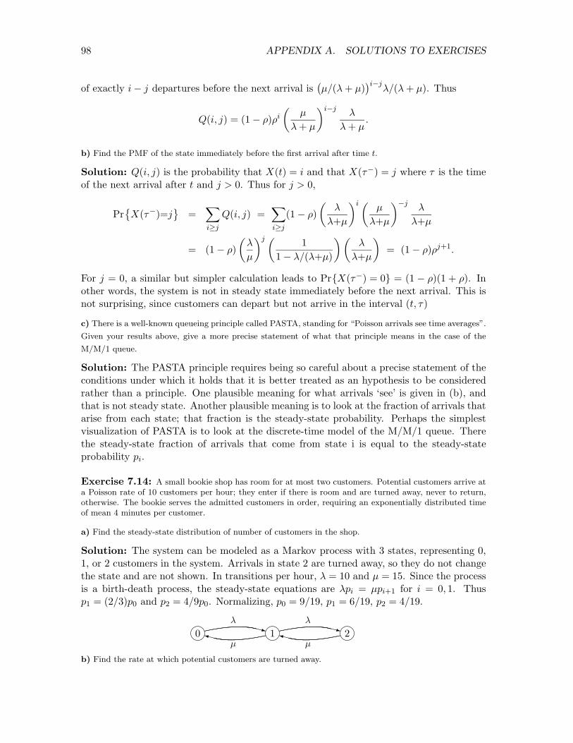
98 APPENDIX A. SOLUTIONS TO EXERCISES
of exactly i� j departures before the next arrival is�µ/(� + µ)
�i�j�/(� + µ). Thus
Q(i, j) = (1� ⇢)⇢i
✓µ
� + µ
◆i�j �
� + µ.
b) Find the PMF of the state immediately before the first arrival after time t.
Solution: Q(i, j) is the probability that X(t) = i and that X(⌧�) = j where ⌧ is the timeof the next arrival after t and j > 0. Thus for j > 0,
Pr�X(⌧�)=j
=
Xi�j
Q(i, j) =Xi�j
(1� ⇢)✓
�
�+µ
◆i✓ µ
�+µ
◆�j �
�+µ
= (1� ⇢)✓
�
µ
◆j ✓ 11� �/(�+µ)
◆✓�
�+µ
◆= (1� ⇢)⇢j+1.
For j = 0, a similar but simpler calculation leads to Pr{X(⌧�) = 0} = (1 � ⇢)(1 + ⇢). Inother words, the system is not in steady state immediately before the next arrival. This isnot surprising, since customers can depart but not arrive in the interval (t, ⌧)
c) There is a well-known queueing principle called PASTA, standing for “Poisson arrivals see time averages”.
Given your results above, give a more precise statement of what that principle means in the case of the
M/M/1 queue.
Solution: The PASTA principle requires being so careful about a precise statement of theconditions under which it holds that it is better treated as an hypothesis to be consideredrather than a principle. One plausible meaning for what arrivals ‘see’ is given in (b), andthat is not steady state. Another plausible meaning is to look at the fraction of arrivals thatarise from each state; that fraction is the steady-state probability. Perhaps the simplestvisualization of PASTA is to look at the discrete-time model of the M/M/1 queue. Therethe steady-state fraction of arrivals that come from state i is equal to the steady-stateprobability pi.
Exercise 7.14: A small bookie shop has room for at most two customers. Potential customers arrive ata Poisson rate of 10 customers per hour; they enter if there is room and are turned away, never to return,otherwise. The bookie serves the admitted customers in order, requiring an exponentially distributed timeof mean 4 minutes per customer.
a) Find the steady-state distribution of number of customers in the shop.
Solution: The system can be modeled as a Markov process with 3 states, representing 0,1, or 2 customers in the system. Arrivals in state 2 are turned away, so they do not changethe state and are not shown. In transitions per hour, � = 10 and µ = 15. Since the processis a birth-death process, the steady-state equations are �pi = µpi+1 for i = 0, 1. Thusp1 = (2/3)p0 and p2 = 4/9p0. Normalizing, p0 = 9/19, p1 = 6/19, p2 = 4/19.
0 1 2n� �
µ µ
n XzXy
n XzXy
b) Find the rate at which potential customers are turned away.

A.7. SOLUTIONS FOR CHAPTER 7 99
Solution: All arrivals in state 2 are turned away, so the average rate at which customersare turned away is 40/19 per hour.
c) Suppose the bookie hires an assistant; the bookie and assistant, working together, now serve each customer
in an exponentially distributed time of mean 2 minutes, but there is only room for one customer (i.e., the
customer being served) in the shop. Find the new rate at which customers are turned away.
Solution: Now � = 10 and µ = 30. There are two states, with p0 = 3/4 and p1 = 1/4.Customers are turned away at rate 10/4, which is somewhat higher than the rate withoutthe assistant.
Exercise 7.16: Consider the job sharing computer system illustrated below. Incoming jobs arrive fromthe left in a Poisson stream. Each job, independently of other jobs, requires pre-processing in system 1 withprobability Q. Jobs in system 1 are served FCFS and the service times for successive jobs entering system1 are IID with an exponential distribution of mean 1/µ1. The jobs entering system 2 are also served FCFSand successive service times are IID with an exponential distribution of mean 1/µ2. The service times in thetwo systems are independent of each other and of the arrival times. Assume that µ1 > �Q and that µ2 > �.Assume that the combined system is in steady state.
System 1µ1
System 2µ2
--
--� Q
1�Q
a) Is the input to system 1 Poisson? Explain.
Solution: The input to system 1 is the splitting of a Poisson process and is thus Poissonof rate �Q.
b) Are each of the two input processes coming into system 2 Poisson? Explain.
Solution: The output of system 1 is Poisson of rate �Q by Burke’s theorem. The otherprocess entering system 2 is also Poisson with rate (1 � Q)�, since it is a splitting of theoriginal Poisson process of rate �. This input to system 2 is independent of the departuresfrom system 1 (since it is independent both of the arrivals and departures from system 1.)Thus the combined process into system 2 is Poisson with rate �
c) Give the joint steady-state PMF of the number of jobs in the two systems. Explain briefly.
Solution: The state X2(t) of system 2 at time t is dependent on the inputs to system 2 upto time t and the services in system 2 up to time t. By Burke’s theorem, the outputs fromsystem 1 at times up to time t are independent of the state X1(t) of system 1 at time t, andthus the inputs to system 2 from system 1 at times up to t are independent of X1(t). Theother input to system 2 is also independent entirely of system 1. Thus X1(t) and X2(t) areindependent. Thus X1(t) and X2(t) are independent and are the states of M/M/1 queuesin steady state at time t.
Pr{X1(t),X2(t) = i, j} = (1� ⇢1)⇢i1(1� ⇢2)⇢j
2,
where ⇢1 = �Q/µ1 and ⇢2 = �/µ2. Note that this independence applies to the states ofsystem 1 and 2 at the same instant t. The processes are not independent, and, for example,X1(t) and X2(t + ⌧) for ⌧ > 0 are not independent.

100 APPENDIX A. SOLUTIONS TO EXERCISES
d) What is the probability that the first job to leave system 1 after time t is the same as the first job that
entered the entire system after time t?
Solution: The first job out of system 1 after t is the same as the first job into system 1 aftert if and only if system 1 is empty at time t. This is also the same as the first job into theoverall system if the first arrival to the entire system goes into system 1. The probabilityof both of these events (which are independent) is thus P1 = Q(1� ⇢1).
e) What is the probability that the first job to leave system 2 after time t both passed through system 1
and arrived at system 1 after time t.
Solution: Let P2 be the probability of this event. This requires, first, that the event in (d)is satisfied, second that system 2 is empty at time t, and, third, that the first job to bypasssytem 1 after the first arrival to system 1 occurs after the service of that first arrival.
This third event is the event that an exponential rv of rate µ1 has a smaller sample valuethan one of rate �(1�Q). The probability of this is µ1/
�µ1 + �(1�Q)
�. Thus
P2 = P1(1� ⇢2)µ1
µ1 + �(1�Q).
Exercise 7.19: Consider the closed queueing network in the figure below. There are three customerswho are doomed forever to cycle between node 1 and node 2. Both nodes use FCFS service and haveexponentially distributed IID service times. The service times at one node are also independent of those atthe other node and are independent of the customer being served. The server at node i has mean servicetime 1/µi, i = 1, 2. Assume to be specific that µ2 < µ1.
�
-
Node 1
µ1
Node 2
µ2
a) The system can be represented by a four state Markov process. Draw its graphical representation and
label it with the individual states and the transition rates between them.
Solution: The three customers are statistically identical, so we can take the number ofcustomers in node 1 (which can be 0, 1, 2, 3) to be the state. In states 1, 2, 3, departuresfrom node 1 take place at rate µ1. In states 0, 1, 2, departures occur from node 2 at rateµ2, and these serve as arrivals to node 1. Thus the process has the following graphicalrepresentation.
0 1 2 3nµ2 µ2 µ2
µ1 µ1 µ1
n XzXy
n XzXy
n XzXy
b) Find the steady-state probability of each state.
Solution: Perhaps surprisingly, this is the same as an M/M/1 queue in which arrivals areturned away when X(t) = 3. In the queue representation, we lose the identity of the three

A.7. SOLUTIONS FOR CHAPTER 7 101
customers, but we need not keep track of them since they are statistically identical. As wesee in the rest of the exercise, the customer identities can be tracked supplementally, sincethe arrivals to node 1 rotate from customer 1 to 2 to 3. Thus each third arrival in the queuerepresentation corresponds to the same customer.
Let ⇢ = µ2/µ1. Then the steady-state process probabilities are p1 = p0⇢; p2 = ⇢2p0, p3 =⇢3p0, where p0 = 1/(1 + ⇢ + ⇢2 + ⇢3).
c) Find the time-average rate at which customers leave node 1.
Solution: Each customer departure from node 1 corresponds to a downward transitionfrom the queue representation, and thus occurs at rate µ1 from each state except 0 of thequeue. Thus in steady state, customers leave node 1 at rate r = (1�p0)µ1. This is also thetime-average rate at which customers leave node 1.
d) Find the time-average rate at which a given customer cycles through the system.
Solution: Each third departure from node 1 is a departure of the same customer, and thiscorresponds to each third downward transition in the queue. Thus the departure rate of agiven customer from queue 1, which is the same as the rotation rate of that customer, isr/3.
e) Is the Markov process reversible? Suppose that the backward Markov process is interpreted as a closed
queueing network. What does a departure from node 1 in the forward process correspond to in the backward
process? Can the transitions of a single customer in the forward process be associated with transitions of a
single customer in the backward process?
Solution: The queueing process is reversible since it is a birth-death process. The backwardprocess from the two node system, however, views each forward departure from node 1 as anarrival to node 1, i.e., a departure from node 2. Customers 1, 2, 3 then rotate in backwardorder, 1, 3, 2, in the backward system. Thus if one wants to maintain the customer order,the system is not reversible. The system, viewed as a closed queueing system in the sense ofSection 7.7.1, is in essence the same as the queueing network here and also abstracts awaythe individual customer identities, so it is again reversible.
102 APPENDIX A. SOLUTIONS TO EXERCISES
A.8 Solutions for Chapter 8
Exercise 8.1: In this exercise, we evaluate Pr{e⌘ | X = a} and Pr{e⌘ | X = b} for binary detectionfrom vector signals in Gaussian noise directly from (8.40) and(8.41).
a) By using (8.40) for each sample value y of Y , show that
E [LLR(Y ) | X=a ] =�(b � a)T(b � a)
2�2.
Hint: Note that, given X = a , Y = a + Z .
Solution: Taking the expectation of (8.40) conditional on X = a ,
E [LLR(Y ) | X=a ] =(b � a)T
�2E
Y � b + a
2
�
=(b � a)T
�2
✓a � b + a
2
◆,
from which the desired result is obvious.
b) Defining � = kb � ak/(2�), show that
E [LLR(Y ) | X=a ] = �2�2.
Solution: The result in (a) can be expressed as E [LLR(Y )] = �kb�ak2/2�2, from whichthe result follows.
c) Show that
VAR [LLR(Y ) |X=a ] = 4�2.
Hint: Note that the fluctuation of LLR(Y ) conditional on X = a is (1/�2)(b � a)TZ .
Solution: Using the hint,
VAR [LLR(Y )] =1�2
(b � a)TE [ZZ T] (b � a)1�2
=1�2
(b � a)T[I](b � a) =1�2kb � ak2,
from which the result follows.
d) Show that, conditional on X = a , LLR(Y ) ⇠ N (�2�2, 4�2). Show that, conditional on X = a ,
LLR(Y )/2� ⇠ N (��, 1).
Solution: Conditional on X = a , we see that Y = a +Z is Gaussian and thus LLR(Y ) isalso Gaussian conditional on X = a . Using the conditional mean and variance of LLR(Y )found in (b) and (c), LLR(Y ) ⇠ N (�2�2, 4�2).
When the rv LLR(Y ) is divided by 2�, the conditional mean is also divided by 2�, and thevariance is divided by (2�)2, leading to the desired result.
Note that LLR(Y )/2� is very di↵erent from LLR(Y /2�). The first scales the LLR and thesecond scales the observation Y . If the observation itself is scaled, the result is a su�cientstatistic and the LLR is unchanged by the scaling.

A.8. SOLUTIONS FOR CHAPTER 8 103
e) Show that the first half of (8.44) is valid, i.e., that
Pr{e⌘ | X=a} = Pr{LLR(Y )� ln ⌘ |X=a} = Q
✓ln ⌘2�
+ �
◆.
Solution: The first equality above is simply the result of a threshold test with the threshold⌘. The second uses the fact in (d) that LLR(Y )/2�, conditional on X = a , is N (��, 1.This is a unit variance Gaussian rv with mean ��. The probability that it exceeds ln ⌘/2�is then Q
�ln(⌘/2� + �
�.
f) By essentially repeating (a) through (e), show that the second half of (8.44) is valid, i.e., that
Pr{e⌘ | X =b} = Q
✓� ln ⌘
2�+ �
◆.
Solution: One can simply rewrite each equation above, but care is needed in observingthat the likelihood ratio requires a convention for which hypothesis goes on top of thefraction. Thus, here the sign of the LLR is opposite to that in parts (a) to (e). This alsomeans that the error event occurs on the opposite side of the threshold.
Exercise 8.3: a) Let Y be the observation rv for a binary detection problem, let y be the observed
sample value. Let v = v(y) be a su�cient statistic and let V be the corresponding random variable. Show
that ⇤(y) is equal to pV |X (v(y) | b)/p
V |X (v(y) | a). In other words, show that the likelihood ratio of a
su�cient statistic is the same as the likelihood ratio of the original observation.
Solution: This is the third statement of Theorem 8.2.8, and we don’t see any way ofimproving on that proof. It relies on the second statement of the theorem, which is furtherinvestigated in Exercise 8.4
b) Show that this also holds for the ratio of probability densities if V is a continuous rv or random vector.
Solution: Repeating the proof of the third statement of Theorem 8.2.8 for the case in whichY and V have densities, we start with the second statement, i.e., pX|Y (x|y) = pX|V (x|v(y)).
pX|Y (1|y)pX|Y (0|y)
=pX|V (1|v(y))pX|V (0|v(y))
fY |X(y |1)pX(1)/fY (y)fY |X(y |0)pX(0)/fY (y))
=fV |X(v(y)|1)pX(1)/fV (v(y)fV |X(v(y)|0)pX(0)/fV (v(y)
,
Where we have used Bayes’ rule on each term. Cancelling terms, we get
fY |X(y |1)fY |X(y |0)
=fV |X(v(y)|1)fV |X(v(y)|0)
.
The left side of this is ⇤(y), so this is the desired result. We see that it is derived simplyby replacing PMF’s with PDF’s, but there are some assumptions made about the densitiesbeing positive. Turning this into a mathematical theorem with precise conditions wouldrequire measure theory, and without that, it is better to rely on common sense applied tosimple models.

104 APPENDIX A. SOLUTIONS TO EXERCISES
Exercise 8.4:
a) Show that if v(y) is a su�cient statistic according to condition 1 of Theorem 8.2.8, then
pX|Y V
�x | y , v(y)
�= p
X|Y (x | y). (A.49)
Solution: Let V (Y ) be the rv with sample values v(y). Note that {Y = y} is the sameevent as {Y = y}
T{V = v(y)}. If Y is discrete and this event has positive probability,
then (A.49) is obvious since the condition on both sides is the same and has positive prob-ability. If Y is a rv with a positive density, then (A.49) is true if the condition Y = y isreplaced with y � � < Y y. Then (A.49) holds if lim�!0(1/�)Pr{y � � < Y y} > 0,which is valid since Y has a positive density. This type of argument can be extended to thecase where Y is a random vector and holds whether or not V (Y ) is a su�cient statistic.This says that X ! Y ! V is Markov, which is not surprising since V is simply a functionof Y .b) Consider the subspace of events conditional on V (y) = v for a given v. Show that for y such thatv(y) = v,
pX|Y V
�x | y , v(y)
�= p
X|V (x | v). (A.50)
Solution: We must assume (as a natural extension of (a)), that V (Y ) is a su�cientstatistic, i.e., that there is a function u such that for each v, u(v) = ⇤(y) for all y suchthat v(y) = v. We also assume that Y = y has positive probabiity or probability density,since the conditional probabilities don’t have much meaning otherwise. Then
pX|Y V
�1 | y , v(y)
�p
X|Y V
�0 | y , v(y)
� =p
X|Y (1 | y)p
X|Y (0 | y)=
p1
p0⇤(y)
=p1
p0u�v(y)
�,
where we first used (A.49), then Bayes’ law, and then the assumption that u(v) is a su�cientstatistic. Since this ratio is the same for all y for which v(y) has the same value, the ratiois a function of v alone,
pX|Y V
�1 | y , v(y)
�p
X|Y V
�0 | y , v(y)
� =p
X|V
�1 | v
�p
X|V
�0 | v
� . (A.51)
Finally, since pX|V (0|v) = 1� pX|V (1|v) and pX|Y V (0|y , v(y)) = 1� pX|Y V (1|y , v(y)), wesee that (A.51) implies (A.50). Note that this says that X ! V ! Y is Markov.
c) Explain why this argument is valid whether Y is a discrete or continuous random vector and whether V
is discrete, continuous or part discrete and part continuous.
Solution: The argument above essentially makes no assumptions about either Y nor Vbeing discrete or having a density. The argument does depend on the assumption that thegiven conditional probabilities are defined.
Exercise 8.5: a) Let Y be a discrete observation random vector and let v(y) be a function of the samplevalues of Y . Show that
pY |V X
�y | v(y), x
�=
pY |X (y | x)
pV |X
�v(y) | x)
. (A.52)

A.8. SOLUTIONS FOR CHAPTER 8 105
Solution: We must assume that pV X (v(y), x) > 0 so that the expression on the left isdefined. Then, using Bayes’ law on Y and V for fixed x on the left side of (A.52),
pY |V X
�y | v(y), x
�=
pV |Y X
�v(y) | yx
�p
Y |X
�y | x
�p
V |X
�v(y) | x
� . (A.53)
Since V is a deterministic function of Y , the first term in the numerator above is 1, so thisis equivalent to (A.52),
b) Using Theorem 8.2.8, show that the above fraction is independent of X if and only if v(y) is a su�cient
statistic.
Solution: Using Bayes’ law on the numerator and denominator of (A.52),
pY |X (y | x)
pV |X
�v(y) | x)
=p
X|Y (x | y) pY (y)p
X|V
�x | v(y)
�pV (v(y)
. (A.54)
If v(y) is a su�cient statistic, then the second equivalent statement of Theorem 8.2.8, i.e.,
pX|Y (x | y) = p
X|V (x | v(y)),
shows that the first terms on the right side of (A.54) cancel, showing that the fractionis independent of x. Conversely, if the fraction is independent of x, then the ratio ofp
X|Y (x|y) to pX|V (x|v(y)), is a function only of y . Since X is binary, this fraction must be
1, establishing the second statement of Theorem 8.2.8.c) Now assume that Y is a continuous observation random vector, that v(y) is a given function, andV = v(Y ) has a probability density. Define
fY |V X
(y | v(y), x) =fY |X (y | x)
fV |X
�v(y) | x
� . (A.55)
One can interpret this as a strange kind of probability density on a conditional sample space, but it is more
straightforward to regard it simply as a fraction. Show that v(y) is a su�cient statistic if and only if this
fraction is independent of x. Hint: Model your derivation on that in (b), modifying (b) as necessary to do
this.
Solution: The trouble with (A.53) can be seen by looking at (A.54). When this is convertedto densities, the joint density of Y , V (Y ) has the same problem as the densities in Example8.2.10. The numerator and denominator of (A.52) are well defined as densities, however,and the argument in (b) carries through as before.
Exercise 8.9: A disease has two strains, 0 and 1, which occur with a priori probabilities p0 and p1 = 1�p0
respectively.
a) Initially, a rather noisy test was developed to find which strain is present for patients with the disease.
The output of the test is the sample value y1 of a random variable Y1. Given strain 0 (X=0), Y1 = 5 + Z1,
and given strain 1 (X=1), Y1 = 1 + Z1. The measurement noise Z1 is independent of X and is Gaussian,
Z1 ⇠ N (0, �2). Give the MAP decision rule, i.e., determine the set of observations y1 for which the decision
is x=1. Give Pr{e | X=0} and Pr{e | X=1} in terms of the function Q(x).
Solution: This is simply a case of binary detection with an additive Gaussian noise rv. Toprevent simply copying the answer from Example 8.2.3, the signal a associated with X = 0

106 APPENDIX A. SOLUTIONS TO EXERCISES
is 5 and the signal b associated with X = 1 is 1. Thus b < a, contrary to the assumption inExample 8.2.3. Looking at that example, we see that (8.27 ), repeated below, is still valid.
LLR(y) =✓
b� a
�2
◆✓y � b + a
2
◆� x(y)=b�<
x(y)=a
ln(⌘).
We can get a threshold test on y directly by first taking the negative of this expression andthen dividing both sides by the positive term (a� b)/�2 to get
y
x(y)=b>
x(y)=a
��2 ln(⌘)a� b
+b + a
2.
We get the same equation by switching the association of X = 1 and X = 0, which alsochanges the sign of the log threshold.
b) A budding medical researcher determines that the test is making too many errors. A new measurement
procedure is devised with two observation random variables Y1 and Y2. Y1 is the same as in (a). Y2, under
hypothesis 0, is given by Y2 = 5 + Z1 + Z2, and, under hypothesis 1, is given by Y2 = 1 + Z1 + Z2. Assume
that Z2 is independent of both Z1 and X, and that Z2 ⇠ N (0, �2). Find the MAP decision rule for x in
terms of the joint observation (y1, y2), and find Pr{e | X=0} and Pr{e | X=1}. Hint: Find fY2|Y1,X
(y2 | y1, 0)
and fY2|Y1,X
(y2 | y1, 1).
Solution: Note that Y2 is simply Y1 plus the noise term Z2, and that Z2 is independent ofX and Y1. Thus, Y2, conditional on Y1 and X is simply N (Y1,�2), which is independent ofX. Thus Y1 is a su�cient statistic and Y2 is irrelevant. Including Y2 does not change theprobability of error.
c) Explain in laymen’s terms why the medical researcher should learn more about probability.
Solution: It should have been clear intuitively that adding an additional observation thatis only a noisy version of what has already been observed will not help in the decision, butknowledge of probability sharpens one’s intuition so that something like this becomes selfevident even without mathematical proof.
d) Now suppose that Z2, in (b), is uniformly distributed between 0 and 1 rather than being Gaussian. We
are still given that Z2 is independent of both Z1 and X. Find the MAP decision rule for x in terms of the
joint observation (y1, y2) and find Pr(e | X=0) and Pr(e | X=1).
Solution: The same argument as in (b) shows that Y2, conditional on Y1, is independentof X, and thus the decision rule and error probability do not change.
e) Finally, suppose that Z1 is also uniformly distributed between 0 and 1. Again find the MAP decision rule
and error probabilities.
Solution: By the same argument as before, Y2, conditional on Y1 is independent of X, soY1 is a su�cient statistic and Y2 is irrelevant. Since Z1 is uniformly distributed between 0and 1, then Y1 lies between 5 and 6 for X = 0 and between 1 and 2 for X = 1. There isthus no possibility of error in this case.
Exercise 8.10: a) Consider a binary hypothesis testing problem, and denote the hypotheses as X =1
and X =�1. Let a = (a1, a2, . . . , an)T be an arbitrary real n-vector and let the observation be a sample

A.8. SOLUTIONS FOR CHAPTER 8 107
value y of the random vector Y = Xa + Z where Z ⇠ N (0, �2In) and In is the n ⇥ n identity matrix.
Assume that Z and X are independent. Find the maximum likelihood decision rule and find the probabilities
of error Pr(e | X=�1) and Pr(e | X=1) in terms of the function Q(x).
Solution: This is a minor notational variation on Example 8.2.4. Since we are interestedin maximum likelihood, ln ⌘ = 0. The ML test, from (8.41), is then
LLR(y) =2aTy
�2
x(y)=1�<
x(y)=�1
0.
The error probabilities, from (8.44), are then
Pr{e | X=1} = Q (�) Pr{e | X=�1} = Q (�) ,
where � = k2ak/(2�).
b) Now suppose a third hypothesis, X =0, is added to the situation of (a). Again the observation randomvector is Y = Xa + Z , but here X can take on values �1, 0, or +1. Find a one dimensional su�cientstatistic for this problem (i.e., a one dimensional function of y from which the likelihood ratios
⇤1(y) =p
Y |X (y | 1)
pY |X (y | 0)
and ⇤�1(y) =p
Y |X (y | �1)
pY |X (y | 0)
can be calculated).
Solution: We have seen that the likelihood ratio for each of these binary decisions dependsonly on the noise in the direction of the di↵erence between the vectors. Since each di↵erenceis a , we conclude that aTy is a su�cient statistic. One can verify this easily by calculating⇤1(y) and ⇤�1(y).
c) Find the maximum likelihood decision rule for the situation in (b) and find the probabilities of error,
Pr(e | X=x) for x = �1, 0, +1.
Solution: For X = 1, an error is made if ⇤1(y) is less than 1. This occurs if aTy < kak2/2and has probability Pr{e | X = 1} = Q(kak/2�). For X = 0, an error occurs if aTy �kak2/2 or if aTy < �kak2/2. Thus Pr{e|X = 0} = 2Q(kak/2�). Finally, for X = �1, anerror occurs if aTy � �kak2/2. Pr{e|X = �1} = Q(kak/2�).
d) Now suppose that Z1, . . . , Zn in (a) are IID and each is uniformly distributed over the interval �2 to
+2. Also assume that a = (1, 1, . . . , 1)T. Find the maximum likelihood decision rule for this situation.
Solution: If X = 1, then each Yi, 1 i n lies between -1 and 3 and the conditionalprobability density of each such point is (1/4)n. Similarly, for X = �1, each Yi lies between-3 and 1. If all Yi are between -1 and +1, then the LLR is 0. If any are above 1, the LLRis 1, and if any are below -1, the LLR is �1. Thus the ML rule is x = 1 if any Yi > 1and x = �1 if any Yi < 1. Everything else (which has aggregate probability 2�n) is ‘don’tcare,’ which by convention is detected as X = 1.
Exercise 8.11: A sales executive hears that one of his salespeople is routing half of his incoming salesto a competitor. In particular, arriving sales are known to be Poisson at rate one per hour. According tothe report (which we view as hypothesis X=1), each second arrival is routed to the competition; thus underhypothesis 1 the interarrival density for successful sales is f(y|X=1) = ye�y; y � 0. The alternate hypothesis
108 APPENDIX A. SOLUTIONS TO EXERCISES
(X=0) is that the rumor is false and the interarrival density for successful sales is f(y|X=0) = e�y; y � 0.Assume that, a priori, the hypotheses are equally likely. The executive, a recent student of stochasticprocesses, explores various alternatives for choosing between the hypotheses; he can only observe the timesof successful sales however.
a) Starting with a successful sale at time 0, let Si be the arrival time of the ith subsequent successful sale.
The executive observes S1, S2, . . . , Sn(n � 1) and chooses the maximum aposteriori probability hypothesis
given this data. Find the joint probability density f(S1, S2, . . . , Sn|X=1) and f(S1, . . . , Sn|X=0) and give
the decision rule.
Solution: The interarrival times are independent conditional each on X = 1 and X = 0.The density of an interarrival interval given X = 1 is Erlang of order 2, with density xe�x,so
fS |X(s1, . . . , sn|1) =nY
i=1
h(si � si�1) exp�(si � si�1)
i= e�sn
nYi=1
�si � si�1
�.
The density of an interarrival interval given X = 0 is exponential, so
fS |X(s1, . . . , sn|0) = e�sn .
The MAP rule, with p0 = p1 is then
LLR(y) = ln(s0) +nX
i=2
ln(si � si�1)x(y)=1
�<
x(y)=0
0. (A.56)
The executive might have based a decision only on the aggregate time for n sales to takeplace, but this would not have been a su�cient statistic for the sequence of sale times, sothis would have yielded a higher probability of error. It is also interesting to note that avery short interarrival interval is weighed very heavily in (A.56), and this is not surprisingsince very short intervals are very improbable under X = 1. The sales person, if bothfraudulent and a master of stochastic processes, would recognize that randomizing the salesto the competitor would make the fraud much more di�cult to detect.
b) This is the same as (a) except that the system is in steady state at time 0 (rather than starting with a
successful sale). Find the density of S1 (the time of the first arrival after time 0) conditional on X=0 and
on X=1. What is the decision rule now after observing S1, . . . , Sn.
Solution: Under X = 1, the last arrival before 0 was successful with probability 1/2 androuted away with probability 1/2. Thus fS1|X(s1|1) = (1/2)e�s1 + (1/2)s1e�s1 . This couldalso be derived as a residual life probability. With this modification, the first term in theLLR of (A.56) would be changed from ln(s1) to ln((s1 + 1)/2).
c) This is the same as (b), except rather than observing n successful sales, the successful sales up to some
given time t are observed. Find the probability, under each hypothesis, that the first successful sale occurs
in (s1, s1 +�], the second in (s2, s2 +�], . . . , and the last in (sN(t), sN(t) +�] (assume � very small). What
is the decision rule now?
Solution: The somewhat artificial use of � here is to avoid dealing with the discreterv N(t) and the density of a random number of rv’s. One can eliminate this artificiality

A.8. SOLUTIONS FOR CHAPTER 8 109
after understanding the solution. Under X = 0, the probability that N(t) = n and Si 2[si, si + �) for 1 i n and sn t (using an approximation for � very small) is
�ne�s1
"nY
i=2
e�(si�si�1)
#e�(t�sn) = �ne�t. (A.57)
The term e�(t�sn) on the left side is the probability of no arrivals in (sn, t], which alongwith the other arrival times specifies that N(t) = n.
Under X = 1, the term e�s1 in (A.57) is changed to (1/2)(s1 +1)e�s1 as we saw in (b). Thefinal term, e�(t�sn) in (A.57) must be changed to the probability of no successful sales in(sn, t] under X = 1. This is (t� sn + 1)e�(t�sn). The term �n cancels out in the likelihoodratio, so the decision rule is
LLR(y) = ln✓
1 + s1
2
◆+ ln(t� sn + 1) +
nXi=2
ln(si � si�1)x(y)=1
�<
x(y)=0
0.
Exercise 8.15: Consider a binary hypothesis testing problem where X is 0 or 1 and a one dimensionalobservation Y is given by Y = X + U where U is uniformly distributed over [-1, 1] and is independent of X.
a) Find fY |X(y | 0), fY |X(y | 1) and the likelihood ratio ⇤(y).
Solution: Note that fY |X is simply the density of U shifted by X, i.e.,
fY |X(y | 0) =⇢
1/2; �1 y 10; elsewhere fY |X(y | 1) =
⇢1/2; 0 y 2
0; elsewhere .
The likelihood ratio ⇤(y) is defined only for �1 y 2 since neither conditional density isnon-zero outside this range.
⇤(y) =fY |X(y | 1)fY |X(y | 0)
=
8<:
0; �1 y < 01; 0 y 11; 1 < y 2
.
b) Find the threshold test at ⌘ for each ⌘, 0 < ⌘ < 1 and evaluate the conditional error probabilities,
q0(⌘) and q1(⌘).
Solution: Since ⇤(y) has finitely many (3) possible values, all values of ⌘ between anyadjacent pair lead to the same threshold test. Thus, for ⌘ > 1, ⇤(y) � ⌘, if and only if (i↵)⇤(y) = 1. Thus x = 1 i↵ 1 < y 2. For ⌘ = 1, x = 1 i↵ ⇤(y) � 1, i.e., i↵ ⇤(y) is 1 or 1.Thus x = 1 i↵ 0 y 2. For ⌘ < 1, �(y) � ⌘ i↵ ⇤(y) is 1 or 1. Thus x = 1 i↵ 0 y 2.Note that the MAP test is the same for ⌘ = 1 and ⌘ < 1, in both cases choosing x = 1 for0 y 2.
Consider q1(⌘) (the error probabiity using a threshold test at ⌘ conditional of X = 1). For⌘ > 1, we have seen that x = 1 (no error) for 1 < y 2. This occurs with probability 1/2given X = 1. Thus q1(⌘) = 1/2 for ⌘ > 1. Also, for ⌘ > 1, x = 0 for �1 y 1. Thusq0(⌘) = 0. Reasoning in the same way for ⌘ 1, we have q1(⌘) = 0 and q0(⌘) = 1/2.

110 APPENDIX A. SOLUTIONS TO EXERCISES
c) Find the error curve u(↵) and explain carefully how u(0) and u(1/2) are found (hint: u(0) = 1/2).
Solution: Each ⌘ > 1 maps into the pair of error probabilities (q0(⌘), q1(⌘)) = (0, 1/2).Similarly, each ⌘ 1 maps into the pair of error probabilities (q0(⌘), q1(⌘)) = (1/2, 0). Theerror curve contains these points and also contains the supremum of the straight lines ofeach slope �⌘ around (0, 1/2) for ⌘ > 1 and around (1/2, 0) for ⌘ 1. The resulting curveis given below.
ss
1/2
q1(⌘)
1 (0, 1)
1(1, 0)
q0(⌘) 1/2Another approach (perhaps more insightful) is to repeat (a) and (b) for the alternativethreshold tests that choose x = 0 in the don’t care cases, i.e., the cases for ⌘ = 1 and0 y 1. It can be seen that Lemma 8.4.1 and Theorem 8.4.2 apply to these alternativethreshold tests also. The points on the straight line between (0, 1/2) and (1/2, 0) canthen be achieved by randomizing the choice between the threshold tests and the alternativethreshold tests.
d) Describe a decision rule for which the error probability under each hypothesis is 1/4. You need not use
a randomized rule, but you need to handle the don’t-care cases under the threshold test carefully.
Solution: The don’t care cases arise for 0 y 1 when ⌘ = 1. With the decision rule of(8.11), these don’t care cases result in x = 1. If half of those don’t care cases are decidedas x = 0, then the error probability given X = 1 is increased to 1/4 and that for X = 0 isdecreased to 1/4. This could be done by random choice, or more easily, by mapping y > 1/2into x = 1 and y 1/2 into x = 0.

A.9. SOLUTIONS FOR CHAPTER 9 111
A.9 Solutions for Chapter 9
Exercise 9.1: Consider the simple random walk {Sn; n � 1} of Section 9.1.1 with Sn = X1 + · · ·+ Xn
and Pr{Xi = 1} = p; Pr{Xi = �1} = 1� p; assume that p 1/2.
a) Show that PrnS
n�1 {Sn � k}o
=hPrnS
n�1 {Sn � 1}oik
for any positive integer k. Hint: Given that
the random walk ever reaches the value 1, consider a new random walk starting at that time and explore
the probability that the new walk ever reaches a value 1 greater than its starting point.
Solution: Since {Sn;n � 1} changes only in increments of 1 or -1, the only way that thewalk can reach a threshold at integer k > 1 (i.e., the only way that the event
Sn�1 {Sn � k}
can occur), is if the walk first eventually reaches the value 1, and then starting from thefirst time that 1 is reached, goes on to eventually reach 2, and so forth onto k.
The probability of eventually reaching 2 given that 1 is reached is the same as the probabilityof eventually reaching 1 starting from 0; this is most clearly seen from the Markov chaindepiction of the simple random walk given in Figure 6.1. Similarly, the probability ofeventually reaching any j starting from j � 1 is again the same, so (using induction if oneinsists on being formal), we get the desired relationship. This relationship also holds forp > 1/2.
b) Find a quadratic equation for y = PrnS
n�1 {Sn � 1}o. Hint: explore each of the two possibilities
immediately after the first trial.
Solution: As explained in Example 5.5.4, y = p + (1� p)y2.
c) For p < 1/2, show that the two roots of this quadratic equation are p/(1 � p) and 1. Argue that
PrnS
n�1 {Sn � 1}o
cannot be 1 and thus must be p/(1� p).
Solution: This is also explained in Example 5.5.4.
d) For p = 1/2, show that the quadratic equation in (c) has a double root at 1, and thus PrnS
n�1 {Sn � 1}o
=
1. Note: this is the very peculiar case explained in Section 5.5.1.
Solution: As explained in Example 5.5.4, the fact that the roots are both 1 means thatPrnS
n�1 {Sn � 1}o
= 1.
e) For p < 1/2, show that p/(1 � p) = exp(�r⇤) where r⇤ is the unique positive root of g(r) = 1 where
g(r) = E⇥erX
⇤.
Solution: Note that g(r) = E⇥erX⇤
= per + (1� p)e�r. The positive root of g(r) = 1 isthe r⇤ > 0 for which
1 = per⇤ + (1� p)e�r⇤ .
This is quadratic in er⇤ (and also in e�r⇤) and is the same equation as in (b) if we substitutey for e�r⇤ . The two solutions are e�r⇤=1 (r⇤=0) and e�r⇤ = p/(1� p) (r⇤ = ln[(1� p)/p]).Thus the unique positive solution for r⇤ is ln[(1�p)/p]. Thus the optimized Cherno↵ boundfor crossing a threshold is satisfied with equality by the simple combinatorial solution in(c).
Exercise 9.2: Consider a G/G/1 queue with IID arrivals {Xi; i � 1}, IID FCFS service times{Yi; i � 0}, and an initial arrival to an empty system at time 0. Define Ui = Yi�1 �Xi for i � 1. (Note:
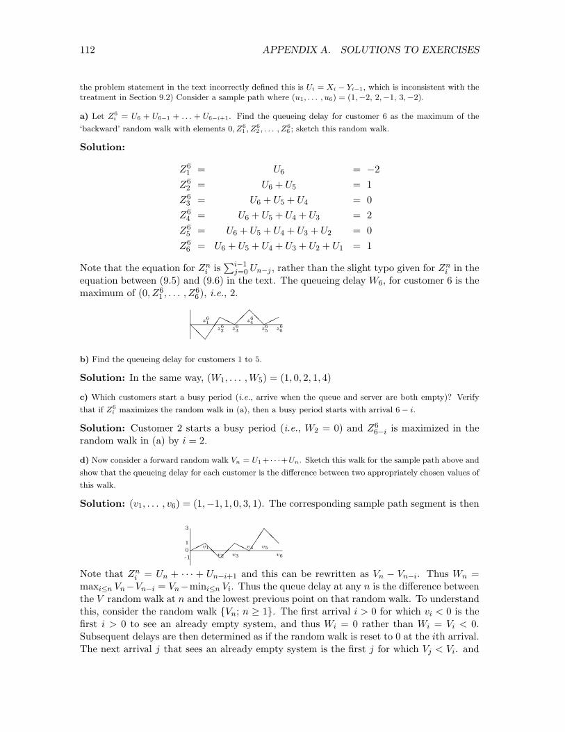
112 APPENDIX A. SOLUTIONS TO EXERCISES
the problem statement in the text incorrectly defined this is Ui = Xi � Yi�1, which is inconsistent with thetreatment in Section 9.2) Consider a sample path where (u1, . . . , u6) = (1,�2, 2,�1, 3,�2).
a) Let Z6i = U6 + U6�1 + . . . + U6�i+1. Find the queueing delay for customer 6 as the maximum of the
‘backward’ random walk with elements 0, Z61 , Z6
2 , . . . , Z66 ; sketch this random walk.
Solution:
Z61 = U6 = �2
Z62 = U6 + U5 = 1
Z63 = U6 + U5 + U4 = 0
Z64 = U6 + U5 + U4 + U3 = 2
Z65 = U6 + U5 + U4 + U3 + U2 = 0
Z66 = U6 + U5 + U4 + U3 + U2 + U1 = 1
Note that the equation for Zni is
Pi�1j=0 Un�j , rather than the slight typo given for Zn
i in theequation between (9.5) and (9.6) in the text. The queueing delay W6, for customer 6 is themaximum of (0, Z6
1 , . . . , Z66), i.e., 2.
@@⌦⌦⌦HH�
�@@��z6
1z62 z6
3
z64
z65 z6
6
b) Find the queueing delay for customers 1 to 5.
Solution: In the same way, (W1, . . . ,W5) = (1, 0, 2, 1, 4)
c) Which customers start a busy period (i.e., arrive when the queue and server are both empty)? Verify
that if Z6i maximizes the random walk in (a), then a busy period starts with arrival 6� i.
Solution: Customer 2 starts a busy period (i.e., W2 = 0) and Z66�i is maximized in the
random walk in (a) by i = 2.
d) Now consider a forward random walk Vn = U1 + · · ·+Un. Sketch this walk for the sample path above and
show that the queueing delay for each customer is the di↵erence between two appropriately chosen values of
this walk.
Solution: (v1, . . . , v6) = (1,�1, 1, 0, 3, 1). The corresponding sample path segment is then
��@@��HH⌦
⌦⌦@@v1
v2 v3
v4 v5v6
0-1
1
3
Note that Zni = Un + · · · + Un�i+1 and this can be rewritten as Vn � Vn�i. Thus Wn =
maxin Vn�Vn�i = Vn�minin Vi. Thus the queue delay at any n is the di↵erence betweenthe V random walk at n and the lowest previous point on that random walk. To understandthis, consider the random walk {Vn; n � 1}. The first arrival i > 0 for which vi < 0 is thefirst i > 0 to see an already empty system, and thus Wi = 0 rather than Wi = Vi < 0.Subsequent delays are then determined as if the random walk is reset to 0 at the ith arrival.The next arrival j that sees an already empty system is the first j for which Vj < Vi. and

A.9. SOLUTIONS FOR CHAPTER 9 113
so forth at each arrival to see an already empty system. Thus the smallest Vj for j nis the last j n to start a new busy period. This is somewhat more intuitive than thebackward random walk, but the backward random walk is the one that connects G/G/1queue-waiting with random walks.
Exercise 9.3: A G/G/1 queue has a deterministic service time of 2 and interarrival times that are 3with probability p < 1/2 and 1 with probability 1� p.
a) Find the distribution of W1, the wait in queue of the first arrival after the beginning of a busy period.
Solution: The service time is always 2 units, so the first arrival after the beginning of abusy period must arrive either after 1 unit of the service is completed or 1 unit after theservice is completed. Thus Pr{W1 = 0} = p and Pr{W1 = 1} = 1� p.
b) Find the distribution of W1, the steady-state wait in queue.
Solution: The rv Ui = Yi+1 � Xi is binary (either 2-1 or 2-3), so Pr{Ui = 1} = p andPr{Ui = �1} = 1�p. The backward random walk is thus a simple random walk. FromTheorem 9.2.1, Pr{W � k} is the probability that the random walk based on {Ui; i � 1}ever crosses k. From (9.2), recognizing that the simple random walk is integer valued,
Pr{W � k} =✓
p
1� p
◆k
.
c) Repeat (a) and (b) assuming the service times and interarrival times are exponentially distributed with
rates µ and � respectively.
Solution: This is an M/M/1 queue. With probability µ/(� + µ), the first arrival appearsafter the initial departure and thus has no wait in the queue. With probability �/(�+µ) thefirst arrival appears before the initial departure, and then waits in queue for an exponentiallydistributed time of rate µ. Thus Pr{W1 > w} = �/(� + µ) exp(�µw) for w � 0.
In steady state, i.e., to find Pr{W > w} = limn!1 Pr{Wn > w}, we recall that the steady-state number N in the system is geometric with pN (n) = (1��/µ)(�/µ)n for n � 0. GivenN = 0 (an event of probability 1 � �/µ), the wait is 0. Given N = n, the wait in thequeue is
Pni=1 Y ⇤
i where each Y ⇤i is exponential with rate µ. Thus for N > 0 (an event
of probability �/µ the wait is a geometrically distributed sum of exponential rv’s. FromExample 2.3.3, this is equivalent to a sum of two Poisson processes, one of rate � and oneof rate µ � � where the first arrival from the µ � � process is geometrically distributed inthe combined µ process. Thus,
Pr{W � w} =�
µexp
�� (µ� �)w
�; for w � 0.
Exercise 9.6: Define �(r) as ln [g(r)] where g(r) = E [exp(rX)]. Assume that X is discrete with possibleoutcomes {ai; i � 1}, let pi denote Pr{X = ai}, and assume that g(r) exists in some open interval (r�, r+)containing r = 0. For any given r, r� < r < r+, define a random variable Xr with the same set of possibleoutcomes {ai; i � 1} as X, but with a probability mass function qi = Pr{Xr = ai} = pi exp[air� �(r)]. Xr
is not a function of X, and is not even to be viewed as in the same probability space as X; it is of interest

114 APPENDIX A. SOLUTIONS TO EXERCISES
simply because of the behavior of its defined probability mass function. It is called a tilted random variablerelative to X, and this exercise, along with Exercise 9.11 will justify our interest in it.
a) Verify thatP
i qi = 1.
Solution: Note that these tilted probabilities are described in Section 9.3.2.
Xi
qi =X
i
pi exp[air � �(r)] =1
g(r)
Xi
pi exp[air] =g(r)g(r)
= 1.
b) Verify that E [Xr] =P
i aiqi is equal to �0(r).
Solution:
E [Xr] =X
i
aipi exp[air � �(r)] =1
g(r)
Xi
aipi exp[air]
=1
g(r)d
dr
Xi
pierai =
g0(r)g(r)
= �0(r). (A.58)
c) Verify that VAR [Xr] =P
i a2i qi � (E [Xr])
2 is equal to �00(r).
Solution: We first calculate the second moment, E⇥X2
r
⇤.
E⇥X2
r
⇤=
Xi
a2i pi exp[air � �(r)] =
1g(r)
Xi
a2i pi exp[air]
=1
g(r)d2
dr2
Xi
pierai =
g00(r)g(r)
. (A.59)
Using (A.58) and (A.59),
VAR [Xr] =g00(r)g(r)
� [g0(r)]2
[g(r)]2=
d2
dr2ln(g(r)) = �00(r).
d) Argue that �00(r) � 0 for all r such that g(r) exists, and that �00(r) > 0 if �00(0) > 0.
Solution: Since �00(r) is the variance of a rv, it is nonnegative. If VAR [X] > 0, then X isnon-atomic, which shows that Xr is non-atomic and thus has a positive variance whereverit exists.
e) Give a similar definition of Xr for a random variable X with a density, and modify (a) to (d) accordingly.
Solution: If X has a density, fX(x), and also has an MGF over some region of r, thenthe tilted variable Xr is defined to have the density fXr(x) = fX(x) exp(xr � �(r)). Thederivations above follow as before except for the need of more care about convergence.
Exercise 9.9: [Details in proof of Theorem 9.3.3] a) Show that the two appearances of ✏ in (9.24) canbe replaced with two independent arbitrary positive quantities ✏1 and ✏2, getting
Pr�Sn � n(�0(r)� ✏1)
� (1� �) exp[�n(r�0(r) + r✏2 � �(r))]. (A.60)

A.9. SOLUTIONS FOR CHAPTER 9 115
Show that if this equation is valid for ✏1 and ✏2, then it is valid for all larger values of ✏1 and ✏2. Hint: Note
that the left side of (9.24) is increasing in ✏ and the right side is decreasing.
Solution: For an arbitrary ✏1 and ✏2, let ✏ = min(✏1, ✏2). For that ✏ and any � > 0, thereis an no such that (9.24) is satisfied for all n � no. Then, using the hint to replace ✏ by✏1 � ✏ on the left of (9.24),
Pr�Sn � n(�0(r)� ✏1)
� Pr
�Sn � n(�0(r)� ✏)
� (1� �) exp[�n(r�0(r) + r✏� �(r))]� (1� �) exp[�n(r�0(r) + r✏2 � �(r))].
This also shows that if (A.60) is satisfied for a given ✏1, ✏2 and n, then it is satisfied for alllarger ✏1, ✏2 for that n.
b) Show that by increasing the required value of no, the factor of (1� �) can be eliminated in (A.60).
Solution: We can rewrite (A.60) as
Pr�Sn � n(�0(r)� ✏1)
� (1� �)enr✏2 exp[�n(r�0(r) + 2r✏2 � �(r))].
This applies for n � no for the no in part (a). Now choose n0o large enough so that both(1� �)enor✏02 � 1 and (A.60) (for the given (✏1, ✏2)) is satisfied. Then for n � n0o,
Pr�Sn � n(�0(r)� ✏1)
� (1� �)enr✏0 exp[�n(r�0(r) + 2r✏2 � �(r))]� exp[�n(r�0(r) + 2r✏2 � �(r))]= exp[�n(r�0(r) + r✏02 � �(r))], (A.61)
where ✏02 = 2✏2. Since ✏2 > 0 is arbitrary, ✏02 > 0 is also arbitrary, with the correspondingchange to n0o.
c) For any r 2 (0, r+), let �1 be an arbitrary number in (0, r+�r), let r1 = r+�1, and let ✏1 = �0(r1)��0(r).Show that there is an m such that for all n � m,
Pr�Sn � n�0(r)
� exp
��n
⇥(r + �1)�
0(r + �1) + (r + �1)✏2 � �(r + �1)⇤
. (A.62)
Using the continuity of � and its derivatives, show that for any ✏ > 0, there is a �1 > 0 so that the right side
of (A.62) is greater than or equal to exp[�n(�0(r)� r�(r) + r✏)].
Solution: Since �0(r) is increasing in r, ✏1 = �0(r1) � �0(r) > 0. Now (A.61) applies forarbitrary r 2 (0, r+) and ✏1, ✏2 (using the appropriate n0o for those parameters). Thus wecan apply (A.61) to r1 and ✏1 as defined above and with ✏2 replacing ✏02.
Pr�Sn � n(�0(r1)� ✏1)
� exp[�n(r1�
0(r1) + r1✏2 � �(r1))]
Replacing �0(r1) � ✏1 on the left with �0(r) and r1 on the right by r + �1, we get (A.62).This is valid for n � m where m is the value of n0o for these modifications of r, ✏1, and ✏2.
Let ✏ > 0 be arbitrary. Since r�0(r) is continuous in r, we see that for all small enough�1, (r + �1)�0(r + �1) r�0(r) + r✏/3. Similarly, ��(r + �1) ��(r) + r✏/3 for all smallenough �1. Finally, for any such small enough �1, we can choose ✏2 > 0 small enough that

116 APPENDIX A. SOLUTIONS TO EXERCISES
(r + �1)✏2 r✏/3. Substituting these inequalities into (A.62), there is an m such that forn � m,
Pr�Sn � n�0(r)
� exp
��n⇥r�0(r) + r✏� �(r)
⇤ ,
thus completing the final details of the proof of Theorem 9.3.3.
Exercise 9.13: Consider a random walk {Sn; n � 1} where Sn = X1 + · · ·Xn and {Xi; i � 1} is asequence of IID exponential rv’s with the PDF f(x) = �e��x for x � 0. In other words, the random walk isthe sequence of arrival epochs in a Poisson process.
a) Show that for �a > 1, the optimized Cherno↵ bound for Pr{Sn � na} is given by
Pr{Sn � na} (a�)ne�n(a��1).
Solution: The moment generating function is g(r) = E⇥eXr⇤
= �/(�� r) for r < �. Thus�(r) = ln g(r) = ln(�/(� � r)) and �0(r) = 1/(� � r). The optimizing r for the Cherno↵bound is then the solution to a = 1/(� � r), which is r = � � 1/a. Using this r in theCherno↵ bound,
Pr{Sn � na} expn ln(
�
�� r)� nra
�= exp[n ln(a�)� n(a�� 1)],
which is equivalent to the desired expression.
b) Show that the exact value of Pr{Sn � na} is given by
Pr{Sn � na} =n�1Xi=0
(na�)i e�na�
i!. (A.63)
Solution: For a Poisson counting process {N(t); t > 0}, the event {Sn > na} is the sameas {N(na) < n} =
Sn�1i=0 {N(na) = i}. Since this is a union of disjoint events,
Pr{Sn > na} =n�1Xi=0
Pr{N(na) = i}
Using the Poisson PMF, the right side of this is equal to the right side of (A.63). Since Sn
is continuous, Pr{Sn > na} = Pr{Sn � na}.c) By upper and lower bounding the quantity on the right of (A.63), show that
(na�)n e�na�
n! a� Pr{Sn � na} (na�)ne�na�
n!(a�� 1).
Hint: Use the term at i = n� 1 for the lower bound and note that the term on the right can be bounded by
a geometric series starting at i = n� 1.
Solution: The lower bound on the left is the single term with i = n � 1 of the sum in(A.63). For the upper bound, rewrite the sum in (b) as
n�1Xi=0
(na�)i e�na�
i!=
(na�)n e�na�
n!
n
na�+
n(n� 1)(na�)2
+ · · ·�
(na�)n e�na�
n!
1a�
+1
(a�)2+ · · ·
�=
(na�)ne�na�
n!(a�� 1).

A.9. SOLUTIONS FOR CHAPTER 9 117
d) Use the Stirling bounds on n! to show that
(a�)n e�n(a��1)
p2⇡n a� exp(1/12n)
Pr{Sn � na} (a�)ne�n(a��1)
p2⇡n (a�� 1)
.
Solution: The Stirling bounds arep
2⇡n⇣n
e
⌘n< n! <
p2⇡n
⇣n
e
⌘ne1/12n.
Substituting these for n! in (c) and cancelling terms gives the desired expression. Note thatthe Cherno↵ bound contains all the factors that vary exponentially with n. Note also thatthe Erlang expression for Sn and the Poisson expression for N(t) are quite simple, but thecorresponding CDF’s are quite messy, and this makes the Cherno↵ bound more attractivein this case.
Exercise 9.14: Consider a random walk with thresholds ↵ > 0, � < 0. We wish to find Pr{SJ � ↵} inthe absence of a lower threshold. Use the upper bound in (9.46) for the probability that the random walkcrosses ↵ before �.
a) Given that the random walk crosses � first, find an upper bound to the probability that ↵ is now crossed
before a yet lower threshold at 2� is crossed.
Solution: Let J1 be the stopping trial at which the walk first crosses either ↵ or �. Let J2
be the stopping trial at which the random walk first crosses either ↵ or 2� (assuming therandom walk continues forever rather than actually stopping at any stopping trial. Notethat if SJ1 � ↵, then SJ2 = SJ1 , but if SJ1 �, then it is still possible to have SJ2 � ↵.In order for this to happen, a random walk starting at trial J1 must reach a threshold of↵� SJ1 before reaching 2� � SJ1 . Putting this into equations,
Pr{SJ2 � ↵} = Pr{SJ1 � ↵}+ Pr{SJ2 � ↵ | SJ1 �} Pr{SJ1 �} Pr{SJ1 � ↵}+ Pr{SJ2 � ↵ | SJ1 �} .
The second term above upper bounds the probability that the RW starting at trial J1
reaches ↵� SJ1 before 2� � SJ1 , given that SJ1 �. Since ↵� SJ1 � ↵� �,
Pr{SJ2 � ↵ | SJ1 �} exp[�r⇤(↵� �)],
Thus,
Pr{SJ2 � ↵} exp(�r⇤↵) + exp[�r⇤(↵� �)].
Note that it is conceivable that SJ1 = SJ2 , i.e., that � and 2� are crossed at the same time.The argument above includes this case, and no further note about it is necessary.
b) Given that 2� is crossed before ↵, upper bound the probability that ↵ is crossed before a threshold at
3�. Extending this argument to successively lower thresholds, find an upper bound to each successive term,
and find an upper bound on the overall probability that ↵ is crossed. By observing that � is arbitrary, show
that (9.46) is valid with no lower threshold.
Solution: Let Jk for each k � 1 be the stopping trial at which ↵ or k� is crossed. By thesame argument as above,
Pr�SJk+1 � ↵
= Pr{SJk � ↵}+ Pr
�SJk+1 � ↵ | SJk k�
Pr{SJk k�}
Pr{SJk � ↵}+ exp[�r⇤(↵� k�)],

118 APPENDIX A. SOLUTIONS TO EXERCISES
Finally, let J1 be the defective stopping time at which ↵ is first crossed. We see from abovethat the event SJ1 > ↵ is the union of the the events SJk � ↵ over all k � 1. We can upperbound this by
Pr{SJ1 � ↵} Pr{SJ1 � ↵}+1X
k=1
Pr�SJk+1 � ↵ | SJk k�
exp[�r⇤↵]1
1� exp[�r⇤�].
Since this is true for all � < 0, it is valid in the limit � ! �1, yielding e�r⇤↵.
The reason why we did not simply take the limit � ! �1 in the first place is that sucha limit would not define a non-defective stopping rule. The approach here is to define thelimit as a union of non-defective stopping rules.
Exercise 9.16: a) Use Wald’s equality to show that if X = 0, then E [SJ ] = 0 where J is the time of
threshold crossing with one threshold at ↵ > 0 and another at � < 0.
Solution: Wald’s equality holds since E [|J |] < 1, which follows from Lemma 9.4.1, whichsays that J has an MGF in an interval around 0. Thus E [SJ ] = XE [J ]. Since X = 0, itfollows that E [SJ ] = 0.
b) Obtain an expression for Pr{SJ � ↵}. Your expression should involve the expected value of SJ conditional
on crossing the individual thresholds (you need not try to calculate these expected values).
Solution: Writing out E [SJ ] = 0 in terms of conditional expectations,
E [SJ ] = Pr{SJ � ↵}E [SJ | SJ � ↵] + Pr{SJ �}E [SJ | SJ �]= Pr{SJ � ↵}E [SJ | SJ � ↵] + [1� Pr{SJ � ↵}]E [SJ | SJ �] .
Using E [SJ ] = 0, we can solve this for Pr{SJ � ↵},
Pr{SJ � ↵} =E [�SJ | SJ �]
E [�SJ | SJ �] + E [SJ | SJ � ↵].
c) Evaluate your expression for the case of a simple random walk.
Solution: A simple random walk moves up or down only by unit steps, Thus if ↵ and � areintegers, there can be no overshoot when a threshold is crossed. Thus E [SJ | SJ � ↵] = ↵
and E [SJ | SJ �] = �. Thus Pr{SJ � ↵} = |�||�|+↵ . If ↵ is non-integer, then a positive
threshold crossing occurs at d↵e and a lower threshold crossing at b�c. Thus, in this generalcase Pr{SJ � ↵} = |b�c|
|b�c|+d↵e .
d) Evaluate your expression when X has an exponential density, fX(x) = a1e��x for x � 0 and fX(x) = a2e
µx
for x < 0 and where a1 and a2 are chosen so that X = 0.
Solution: Let us condition on J = n, Sn � ↵, and Sn�1 = s, for s < ↵. The overshoot,V = SJ�↵ is then V = Xn +s�↵. Because of the memoryless property of the exponential,the density of V , conditioned as above, is exponential and fV (v) = �e��v for v � 0. This

A.9. SOLUTIONS FOR CHAPTER 9 119
does not depend on n or s, and is thus the overshoot density conditioned only on SJ � ↵.Thus E [SJ | J � ↵] = ↵ + 1/�. In the same way, E [SJ | SJ �] = � � 1/µ. Thus
Pr{SJ � ↵} =|�|+ µ�1
↵ + ��1 + |�|+ µ�1.
Note that it is not necessary to calculate a1 or a2.
Exercise 9.23: Suppose {Zn; n � 1} is a martingale. Show that
E⇥Zm | Zni , Zni�1 , . . . , Zn1
⇤= Zni for all 0 < n1 < n2 < . . . < ni < m.
Solution: First observe from Lemma 9.6.5 that for ni < m,
E [Zm | Zni , Zni�1, Zni�2, . . . , Z1] = Zni .
This is valid for every sample value of every conditioning variable. Thus consider Zni�1 forexample. Since this equation has the same value for each sample value of Zni�1, the expectedvalue of this conditional expectation over Zni�1 is E [Zm | Zni , Zni�2, . . . , Z1] = Zni . In thesame way, any subset of these conditioning rv’s could be removed, leaving us with thedesired form.
Exercise 9.26: This exercise uses a martingale to find the expected number of successive trials E [J ]until some fixed pattern, a1, a2, . . . , ak, of successive binary digits occurs within a sequence of IID binaryrandom variables X1, X2, . . . (see Example 4.5.1 and Exercise 5.35 for alternative approaches). We take thestopping time J to be the smallest n for which (Xn�k+1, . . . , Xn) = (a1, . . . , ak). A mythical casino andsequence of gamblers who follow a prescribed strategy will be used to determine E [J ]. The outcomes of theplays (trials), {Xn; n � 1} at the casino is a binary IID sequence for which Pr{Xn = i} = pi for i 2 {0, 1}
If a gambler places a bet s on 1 at play n, the return is s/p1 if Xn = 1 and 0 otherwise. With a bet s on 0,the return is s/p0 if Xn = 0 and 0 otherwise; i.e., the game is fair.
a) Assume an arbitrary choice of bets on 0 and 1 by the various gamblers on the various trials. Let Yn be
the net gain of the casino on trial n. Show that E [Yn] = 0. Let Zn = Y1 + Y2 + · · · + Yn be the aggregate
gain of the casino over n trials. Show that for any given pattern of bets, {Zn; n � 1} is a martingale.
Solution: The net gain of the casino on trial n is the sum of the gains on each gambler. Ifa gambler bets s on outcome 1, the expected gain for the casino is s�p1s/p1 = 0. Similarly,it is 0 for a bet on outcome 0. Since the expected gain from each gambler is 0, independentof earlier gains, we have E [Yn|Yn�1 . . . , Y1] = 0. As seen in Example 9.6.3, this implies that{Zn; n � 1} is a martingale.b) In order to determine E [J ] for a given pattern (a1, a2, . . . , ak), we program our gamblers to bet as follows:
i) Gambler 1 has an initial capital of 1 which is bet on a1 at trial 1. If X1 = a1, the capital grows to 1/pa1 ,all of which is bet on a2 at trial 2. If X2 = a2, the capital grows to 1/(pa1pa2), all of which is bet on a3 attrial 3. Gambler 1 continues in this way until either losing at some trial (in which case he leaves with nomoney) or winning on k successive trials (in which case he leaves with 1/[pa1 . . . pak ]).
ii) Gambler `, for each ` > 1, follows the same strategy, but starts at trial `. Note that if the string(a1, . . . , ak) appears for the first time at trials n�k+1, n�k+2, . . . , n, i.e., if J = n, then gambler n�k +1leaves at time n with capital 1/[p(a1) . . . p(ak)] and gamblers j < n � k + 1 have all lost their capital. Wewill come back later to investigate the capital at time n for gamblers n� k + 2 to n.
First consider the string a1=0, a2=1 with k = 2. Find the sample values of Z1, Z2, Z3 for the sample
sequence X1 = 1, X2 = 0, X3 = 1, . . . . Note that gamblers 1 and 3 have lost their capital, but gambler 2

120 APPENDIX A. SOLUTIONS TO EXERCISES
now has capital 1/p0p1. Show that the sample value of the stopping time for this case is J = 3. Given an
arbitrary sample value n � 2 for J , show that Zn = n� 1/p0p1.
Solution: Since gambler 1 bets on 0 at the first trial and X1 = 1, gambler 1 loses andZ1 = 1. At trial 2, gambler 2 bets on 0 and X2 = 0. Gambler 2’s capital increases from1 to 1/p0 so Y2 = 1 � 1/p0. Thus Z2 = 2 � 1/p0. On trial 3, gambler 1 is broke anddoesn’t bet, gambler 2’s capital increases from 1/p0 to 1/p0p1 and gambler 3 loses. ThusY3 = 1 + 1/p0 � 1/p0p1 and Z3 = 3 � 1/p0p1. It is preferable here to look only at thecasino’s aggregate gain Z3 and not the immediate gain Y3. In aggregate, the casino keepsall 3 initial bets, and pays out 1/p0p1.
J = 3 since (X2,X3) = (a1, a2) = (0, 1) and this is the first time that the pattern (0, 1)has appeared. For an arbitrary sample value n for J , note that each gambler before n� 1loses unit capital, gambler n � 1 retires to Maui with capital increased from 1 to 1/p0p1,and gambler n loses. Thus the casino has n� 1/p0p1 as its gain.
c) Find E [ZJ ] from (a). Use this plus (b) to find E [J ]. Hint: This uses the special form of the solution in
(b), not the Wald equality.
Solution: The casino’s expected gain up to each time n is E [Zn] = 0, so it follows thatE [ZJ ] = 0 (It is easy to verify that the condition in 9.104 is satisfied in this case). We sawin (b) that E [Zn | J = n] = n � 1/p0p1, so E [ZJ ] = E [J ] � 1/p0p1. Thus E [J ] = 1/p0p1.Note that this is the mean first passage time for the same problem in Exercise 4.28. Theapproach there was simpler than this for this short string. For long strings, the approachhere will be simpler.
d) Repeat parts b) and c) using the string (a1, . . . , ak) = (1, 1) and initially assuming (X1X2X3) = (011).
Be careful about gambler 3 for J = 3. Show that E [J ] = 1/p21 + 1/p1.
Solution: This is almost the same as (b) except that here gambler 3 wins at time 3. Inother words, since a1 = a2, gamblers 2 and 3 both bet on 1 at time 3. As before, J = 3 forthis sample outcome. We also see that for J equal to an arbitrary n, gamblers n� 1 and nboth bet on 1 and since Xn = 1, both win. Thus E [J ] = 1/p2
1 + 1/p1.
e) Repeat parts b) and c) for (a1, . . . , ak) = (1, 1, 1, 0, 1, 1).
Solution: Given that J = n, we know that (Xn�5, . . . ,Xn) = (111011) so gambler n � 5leaves with 1/p5
1p0 and all previous gamblers lose their capital. For the gamblers after n�5,note that gambler n makes a winning bet on 1 at time n and gambler n� 1 makes winningbets on (1, 1) at times (n�1, n). Thus the casino wins n�1/p5
1p0�1/p1�1/p21. Averaging
over J , we see that E [J ] = 1/(p51p0) + 1/p1 + 1/p2
1. In general, we see that, given J = n,gambler n wins if a1 = ak, gambler 2 wins if (a1, a2) = (ak�1, ak) and so forth.f) Consider an arbitrary binary string a1, . . . , ak and condition on J = n for some n � k. Show that thesample capital of gambler ` is then equal to
• 0 for ` < n� k.
• 1/[pa1pa2 · · · pak ] for ` = n� k + 1.
• 1/[pa1pa2 · · · pai ] for ` = n� i + 1, 1 i < k if (a1, . . . , ai) = (ak�i+1, . . . , ak).
• 0 for ` = n� i + 1, 1 i < k if (a1, . . . , ai) 6= (ak�i+1, . . . , ak).
Verify that this general formula agrees with parts (b), (d), and (e).

A.9. SOLUTIONS FOR CHAPTER 9 121
Solution: Gambler ` for ` n � k bets (until losing a bet) on a1, a2, . . . , ak. Since thefirst occurrence of (a1, . . . , ak) occurs at n, we see that each of these gamblers loses at somepoint and thus is reduced to 0 capital at that point and stays there. Gambler n�k +1 betson a1, . . . , ak at times n�k+1, . . . , n and thus wins each bet for J = n. Finally, gambler` = n� i+1 bets (until losing) on a1, a2, . . . , ai at times n� i+1 to n. Since J = n impliesthat Xn�k+1, . . . ,Xn = a1, . . . ak, gambler n� i + 1 is successful on all i bets if and only if(a1, . . . , ai) = (ak�i+1, . . . , ak).
For (b), gambler n is unsuccessful and in (d), gambler n is successful. In (e), gamblers n�1and n are each successful. It might be slightly mystifing at first that conditioning on J isenough to specify what happens to each gambler after time n�k+1, but the sample valuesof Xn�k+1 to Xn are specified by J = n, and the bets of the gamblers are also specified.
g) For a given binary string (a1, . . . , ak), and each j, 1 j k let Ij = 1 if (a1, . . . , aj) = (ak�j+1, . . . , ak)and let Ij = 0 otherwise. Show that
E [J ] =kX
i=1
IiQi`=1 pa`
.
Note that this is the same as the final result in Exercise 5.35. The argument is shorter here, but more
motivated and insightful there. Both approaches are useful and lead to simple generalizations.
Solution: The ith term in the above expansion is the capital of gambler n� i + 1 at timen. The final term at i = k corresponds to the gambler who retires to Maui and Ik = 1 inall cases. How many other terms are non-zero depends on the choice of string. These otherterms can all be set to zero by choosing a string for which no prefix is equal to the su�x ofthe same length.
Exercise 9.27: a) This exercise shows why the condition E [|ZJ |] < 1 is required in Lemma 9.8.4. Let
Z1 = �2 and, for n � 1, let Zn+1 = Zn[1 + Xn(3n + 1)/(n + 1)] where X1, X2, . . . are IID and take on the
values +1 and �1 with probability 1/2 each. Show that {Zn; n � 1} is a martingale.
Solution: From the definition of Zn above,
E [Zn | Zn�1, Zn�2, . . . , Z1] = E [Zn�1[1 + Xn�1(3n� 2)/n] | Zn�1, . . . , Z1] .
Since the Xn are zero mean and IID, this is just E [Zn�1 | Zn�1 . . . , Z1], which is Zn�1. Wealso must show that E [|Zn|] < 1 for each n. Note that
|Zn| |Zn�1|[1 + (3n� 2)/n] 4|Zn�1|
Thus for each n, |Zn| is bounded (although the bound is rapidly increasing in n), so E [|Zn|] <1 for each n. It follows that {Zn; n � 1} is a martingale.
b) Consider the stopping trial J such that J is the smallest value of n > 1 for which Zn and Zn�1 have
the same sign. Show that, conditional on n < J , Zn = (�2)n/n and, conditional on n = J , ZJ =
�(�2)n(n� 2)/(n2 � n).
Solution: It can be seen from the iterative definition of Zn that Zn and Zn�1 have di↵erentsigns if Xn�1 = �1 and have the same sign if Xn�1 = 1. Thus the stopping trial is thesmallest trial n � 2 for which Xn�1 = 1. Thus for n < J , we must have Xi = �1 for

122 APPENDIX A. SOLUTIONS TO EXERCISES
1 i < n. For n = 2 < J , X1 must be �1, so from the formula above, Z2 = Z1[1�4/2] = 2.Thus Zn = (�2)n/n for n = 2 < J . We can use induction now for arbitrary n < J . Thusfor Xn = �1,
Zn+1 = Zn
1� 3n + 1
n + 1
�=
(�2)n
n
�2nn + 1
=(�2)n+1
n + 1.
The remaining task is to compute Zn for n = J . Using the result just derived for n = J � 1and using XJ�1 = 1,
ZJ = ZJ�1
1 +
3(J�1) + 1J
�=
(�2)J�1
J � 14J � 2
J=
�(�2)J(2J � 1)J(J � 1)
.
c) Show that E [|ZJ |] is infinite, so that E [ZJ ] does not exist according to the definition of expectation, and
show that limn!1 E [Zn|J > n] Pr{J > n} = 0.
Solution: We have seen that J = n if and only if Xi = �1 for 1 i n�2 and XJ�1 = 1.Thus Pr{J = n} = 2�n+1 so
E [|ZJ |] =1X
n=2
2�n+1 · 2n(2n� 1)n(n� 1)
=1X
n=2
2(2n� 1)n(n� 1)
�1X
n=2
4n
= 1, (i)
since the harmonic series diverges.
Finally, we see that Pr{J > n} = 2�n+1 (since this event occurs if and only if Xi = �1 for1 i < n). Thus
E [Zn | J > n] Pr{J > n} =2�n+1(�2)n
n=
2(�1)n
n! 0 .
This martingale and stopping rule gives an example where the condition E [|YJ |] is neededin Lemma 9.8.4. Note that E [YJ ], if it exists, is limn!1
P1i=1 E [ZJ=i] Pr{J=i}. For this
example, this is the alternating version of the harmonic series in (i), which converges in theCauchy sense but not in the usual sense. Exercise 1.8 provides a reminder of why this seriesis defined to be nonexistant, i.e., of why the condition E [|YJ |] < 1 is needed.
Exercise 9.31: Prove Corollaries 9.9.3 to 9.9.5, i.e., prove the following three statements:
a) Let {Zn; n � 1} be a martingale with E⇥Z2
n
⇤< 1 for all n � 1. Then
Pr
⇢max
1nm|Zn| � b
�
E⇥Z2
m
⇤b2
; for all integer m � 2, and all b > 0. (A.64)
Hint: First show that {Z2n; n � 1} is a submartingale.
Solution: Z2n is a convex function of Zn and E
⇥Z2
n
⇤< 1 for all n � 1. Thus, from
Theorem 9.7.4, {Z2n; n � 1} is a submartingale. Applying the submartingale inequality to
{Z2n; n � 1},
Pr⇢
max1nm
Z2n � a
�
E⇥Z2
m
⇤a
.
Substituting b2 for a, this becomes (A.64).

A.9. SOLUTIONS FOR CHAPTER 9 123
b) [Kolmogorov’s random walk inequality] Let {Sn; n � 1} be a random walk with Sn = X1 + · · · + Xn
where {Xi; i � i} is a set of IID random variables with mean X and variance �2. Then for any positiveinteger m and any ✏ > 0,
Pr
⇢max
1nm|Sn � nX| � m✏
� �2
m✏2. (A.65)
Hint: Firt show that {Sn � nX; n � 1} is a martingale.
Solution: Let Zn = Sn � nX. Then {Zn; n � 1} is a martingale as shown in Example9.6.2. E
⇥Z2
m
⇤= m�2, so using (A.64) with m✏ substituted for b, we get (A.65).
c) Let {Sn; n � 1} be a random walk, Sn = X1+· · ·+Xn, where each Xi has mean X < 0 and semi-invariantmoment generating function �(r). For any r > 0 such that 0 < �(r) < 1, and for any ↵ > 0. show that
Pr
⇢max
1inSi � ↵
� exp{�r↵ + n�(r)}. (A.66)
Hint: First show that {erSn ; n � 1} is a submartingale.
Solution: Again let Zn = Sn�nX, so {Zn, n � 1} is a martingale. Then erSn = erZn+rnX
and we see by di↵erentiating twice with respect to Zn that erSn is a convex function ofZn. Thus by Theorem 9.7.4, {erSn ; n � 1} is a submartingale. Thus by the Kolmogorovsubmartingale inequality,
Pr⇢
max1in
erSi � a
�
E⇥erSn
⇤a
. (A.67)
Now E⇥erSn
⇤= [gX(r)]n = en�(r). Substituting er↵ for a, (A.67) becomes (A.66)
Exercise 9.36: (Kelly’s horse-racing game) An interesting special case of this simple theory ofinvestment is the horse-racing game due to J. Kelly and described in [5]. There are ` � 1 horses in a raceand each horse j wins with some probability p(j) > 0. One and only one horse wins, and if j wins, thegambler receives r(j) > 0 for each dollar bet on j and nothing for the bets on other horses. In other words,the price-relative X(j) for each j, 1 j ` � 1, is r(j) with probability p(j) and 0 otherwise. For cash,X(`) = 1.
The gambler’s allocation of wealth on the race is denoted by �(j) on each horse j with �(`) kept in cash. Asusual,
Pj �(j) = 1 and �(j) � 0 for 1 j `. Note that X(1), . . . , X(` � 1) are highly dependent, since
only one has a nonzero sample value in any race.
a) For any given allocation ��� find the expected wealth and the expected log-wealth at the end of a race for
unit initial wealth.
Solution: With probability p(j), horse j wins and the resulting value of W1(���) is �(j)r(j)+�(`). Thus
E [W1(���)] =`�1Xj=1
p(j)⇥�(j)r(j) + �(`)
⇤,
E [L1(���)] =`�1Xj=1
p(j) ln⇥�(j)r(j) + �(`)
⇤.
b) Assume that a statistically identical sequence of races are run, i.e., X 1,X 2, . . . , are IID where each
Xn =�Xn(1), . . . , Xn(`)
�T. Assuming unit initial wealth and a constant allocation ��� on each race, find the
expected log-wealth E [Ln(���)] at the end of the nth race and express it as nE [Y (���)].
124 APPENDIX A. SOLUTIONS TO EXERCISES
Solution: Using (9.128) to express E [Ln(���)] as nE [Y (���)], we have
E [Y (���)] =`�1Xj=1
p(j) ln⇥�(j)r(j) + �(`)
⇤. (A.68)
c) Let ���⇤ maximize E [Y (���)]. Use the necessary and su�cient condition (9.136) on ���⇤ for horse j, 1 j < `to show that �⇤(j) can be expressed in the following two equivalent ways; each uniquely specifies each �⇤(j)in terms of �⇤(`).
�⇤(j) � p(j)� �⇤(`)r(j)
; with equality if �⇤(j) > 0 (A.69)
�⇤(j) = maxn
p(j)��⇤(`)r(j)
, 0o
. (A.70)
Solution: The necessary and su�cient condition for ���⇤ in (9.136) for horse j is
E
X(j)P
k �⇤(k)X(k)
� 1; with equality if �⇤(j) > 0.
In the event that horse j wins, X(j) = r(j) while X(k) = 0 for horses k 6= j. Also X(`) = 1.Thus in the event that horse j wins, X(j)P
k �⇤(k)X(k) = r(j)�⇤(j)r(j)+�⇤(`) . If any other horse wins,
X(j)Pk �⇤(k)X(k) = 0. Thus, since j wins with probability p(j),
E
X(j)P
k �⇤(k)X(k)
�=
p(j) r(j)�⇤(j)r(j) + �⇤(`)
1; with equality if �⇤(j) > 0. (A.71)
Rearranging this inequality yields (A.69); (A.70) is then easily verified by looking separatelyat the cases �⇤(j) > 0 and �⇤(j) = 0.
Solving for �⇤(`) (which in turn specifies the other components of ���⇤) breaks into 3 special cases which aretreated below in parts d), e), and f) respectively. The first case, in (d), shows that if
Pj<` 1/r(j) < 1, then
�⇤(`) = 0. The second case, in (e), shows that ifP
j<` 1/r(j) > 1, then �⇤(`) > minj(p(j)r(j), with thespecific value specified by the unique solution to (A.73). The third case, in (f), shows that if
Pj<` 1/r(j) = 1,
then �⇤(`) is nonunique, and its set of possible values occupy the range [0, minj(p(j)r(j)].
d) Sum (A.69) over j to show that if �⇤(`) > 0, thenP
j<` 1/r(j) � 1. Note that the logical obverse of this
is thatP
j<` 1/r(j) < 1 implies that �⇤(`) = 0 and thus that �⇤(j) = p(j) for each horse j.
Solution: Summing (A.69) over j < ` and using the fact thatP
j<` �⇤(j) = 1� �⇤(`), weget
1� �⇤(`) � 1� �⇤(`)Xj<`
1/r(j).
If �⇤(`) > 0, this shows thatP
j 1/r(j) � 1. The logical obverse is that ifP
j 1/r(j) < 1,then �⇤(`) = 0. This is the precise way of saying that if the returns on the horses aresu�ciently large, then no money should be retained in cash.
When �⇤(`) = 0 is substituted into (A.69), we see that each �⇤(j) must be positive and thusequal to p(j). This is very surprising, since it says that the allocation of bets does not depend

A.9. SOLUTIONS FOR CHAPTER 9 125
on the rewards r(j) (so long as the rewards are large enough to satisfyP
j 1/r(j) < 1). Thiswill be further explained by example in (g).e) In (c), �⇤(j) for each j < ` was specified in terms of �⇤(`); here you are to use the necessary and su�cientcondition (9.136) on cash to specify �⇤(`). More specifically, you are to show that �⇤(`) satisfies each of thefollowing two equivalent inequalities:
Xj<`
p(j)�⇤(j)r(j) + �⇤(`)
1; with equality if �⇤(`) > 0 (A.72)
Xj<`
p(j)
max⇥p(j)r(j), �⇤(`)
⇤ 1; with equality if �⇤(`) > 0. (A.73)
Show from (A.73) that if �⇤(`) p(j)r(j) for each j, thenP
j 1/r(j) 1. Point out that the logical obverse
of this is that ifP
j 1/r(j) > 1, then �⇤(`) > minj(p(j)r(j). Explain why (A.73) has a unique solution for
�⇤(`) in this case. Note that �⇤(j) = 0 for each j such that p(j)r(j) < �⇤(`).
Solution: The necessary and su�cient condition for cash (investment `) is
E
X(`)P
k �⇤(k)X(k)
� 1; with equality if �⇤(`) > 0. (A.74)
In the event that horse j wins, X(`) has the sample value 1 andP
k �⇤(k)X(k) has thesample value �⇤(j)r(j)+�⇤(`). Taking the expectation by multiplying by p(j) and summingover j < `, (A.74) reduces to (A.72). Now if we multiply both sides of (A.70) by r(j) andthen add �⇤(`) to both sides, we get
�⇤(j)r(j) + �⇤(`) = max⇥p(j)r(j), �⇤(`)
⇤,
which converts (A.72) into (A.73). Now assume that �⇤(`) p(j)r(j) for each j. Thenthe max in the denominator of the left side of (A.73) is simply p(j)r(j) for each j and(A.73) becomes
Pj<` 1/r(j) 1. The logical obverse is that
Pj<` 1/r(j) > 1 implies that
�⇤(`) > minj�p(j)r(j)
�, as was to be shown.
Finally, we must show that ifP
j<` 1/r(j) > 1, then (A.73) has a unique solution for �⇤(`).The left side of (A.73), viewed as a function of �⇤(`), is
Pj<` 1/r(j) > 1 for �⇤(`) =
minj�p(j)r(j)
�. This function is continuous and strictly decreasing with further increases
in �⇤(`) and is less than or equal to 1 at �⇤(`) = 1. Thus there must be a unique value of�⇤(`) at which (A.73) is satisfied.
It is interesting to observe from (A.70) that �⇤(j) = 0 for each j such that p(j)r(j) �⇤(`).In other words, no bets are placed on any horse j for which E [X(j)] < �⇤(`). This is inmarked contrast to the case in (d) where the allocation does not depend on r(j) (withinthe assumed range).
f) Now consider the case in whichP
j<` 1/r(j) = 1. Show that (A.73) is satisfied with equality for each
choice of �⇤(`), 0 �⇤(`) minj<` p(j)r(j).
Solution: Note that max⇥p(j)r(j), �⇤(`)
⇤= p(j)r(j) over the given range of �⇤(`), so the
left side of (A.73) isP
j<` 1/r(j) = 1 over this range. Thus the inequality in (A.73) issatisfied for all �⇤(`) in this range. From (A.204), �⇤(j) = p(j)��⇤(`)/r(j) can be used foreach j < `, to see that all the necessary and su�cient conditions are satisfied for maximizingE [Y (���)].

126 APPENDIX A. SOLUTIONS TO EXERCISES
g) Consider the special case of a race with only two horses. Let p(1) = p(2) = 1/2. Assume that r(1) andr(2) are large enough to satisfy 1/r(1) + 1/r(2) < 1; thus no cash allotment is used in maximizing E [Y (���)].With �(3) = 0, we have
E [Y (���)] =12
ln[�(1)r(1)] +12
ln[�(2)r(2)] =12
ln[�(1)r(1)�1� �(1)
�r(2)]. (A.75)
Use this equation to give an intuitive explanation for why �⇤(1) = 1/2, independent of r(1) and r(2)).
Solution: Suppose that r(1) >> r(2). Choosing �(1) to be large so as to enhance the profitwhen horse 1 wins is counter-productive, since (A.75) shows that there is a correspondingloss when horse 2 wins. This gain and loss cancel each other in the expected log wealth. Toview this slightly di↵erently, if each horse wins n/2 times, Wn is given by
Wn =��(1)
�n/2�1� �(1)�n/2�
r(1)�n/2�
r(2)�n/2
,
which again makes it clear that �⇤(1) does not depend on r(1) and r(2).
h) Again consider the special case of two horses with p(1) = p(2) = 1/2, but let r(1) = 3 and r(2) = 3/2.
Show that ���⇤ is nonunique with (1/2, 1/2, 0) and (1/4, 0, 3/4) as possible values. Show that if r(2) > 3/2,
then the first solution above is unique, and if r(2) < 3/2, then the second solution is unique, assuming
p(1) = 1/2 and r(1) = 3 throughout. Note: When 3/2 < r(2) < 2, this is an example where an investment
in used to maximize log-wealth even though E [X(2)] = p(2)r(2) < 1, i.e., horse 2 is a lousy investment, but
is preferable to cash in this case as a hedge against horse 1 losing.
Solution: Approach 1: Substitute ���⇤ = (1/2, 1/2, 0)T and then (1/4, 0, 3/4)T into thenecessary and su�cient conditions; each satisfies those conditions. Approach 2: Note that1/r(1) + 1/r(2) = 1. Thus, from (f), each of these values is satisfied.
Both choices of ���⇤ here lead to the same rv, i.e., Y (���⇤) = ln[3/2] for the event that horse 1wins and Y (���⇤) = ln[3/4] for the event that horse 2 wins. In other words, the maximizingrv Y (���⇤) is uniquely specified, even though ���⇤ is not unique. All points on the straight linebetween these two choices of ���⇤, i.e., (1/2� ↵, 1/2� 2↵, 3↵)T for 0 ↵ 1/4 also lead tothe same optimizing Y (���⇤).
For r(2) > 3/2, we have 1/r(1) + 1/r(2) < 1, so from (d), the solution (1/2, 1/2, 0) is validand in this case unique. This can also be seen by substituting this choice of ���⇤ into thenecessary and su�cient conditions, first with r(2) > 3/2 and then with r(2) < 3/2.
From (e), the choice ���⇤ = (1/4, 0, 3/4) is the unique solution for 1/r(1) + 1/r(2) > 0, i.e.,for r(2) < 3/2. This can be recognized as the allocation that maximizes E [Y (�)] for thetriple-or-nothing investment.
i) For the case whereP
j<` 1/r(j) = 1, define q(j) = 1/r(j) as a PMF on {1, . . . , ` � 1}. Show that
E [Y (���⇤)] = D(p k q) for the conditions of (f). Note: To interpret this, we could view a horse race where
each horse j has probability q(j) of winning the reward r(j) = 1/q(j) as a ‘fair game’. Our gambler, who
knows that the true probabilities are {p(j); 1 j < `}, then has ‘inside information’ if p(j) 6= q(j), and can
establish a positive rate of return equal to D(p k q).
Solution: From (f),⇣p(1), . . . , p(`� 1), 0
⌘T
is one choice for the optimizing ���⇤. Using thischoice,
E [Y (���⇤)] =Xj<`
p(j) ln[p(j)r(j)] = D(p k q).

A.9. SOLUTIONS FOR CHAPTER 9 127
To further clarify the notion of a fair game, put on rose-colored glasses to envision a racetrack that simply accumulates the bets from all gamblers and distributes all income to thebets on the winning horse. In this sense, q(j) = 1/r(j) is the ‘odds’ on horse j as establishedby the aggregate of the gamblers. Fairness is not a word that is always used the same way,and here, rather than meaning anything about probabilities and expectations, it simplyrefers to the unrealistic assumption that neither the track nor the horse owners receive anyexpected return from the betting.
Exercise 9.42: Let {Zn; n � 1} be a martingale, and for some integer m, let Yn = Zn+m � Zm.
a) Show that E [Yn | Zn+m�1 = zn+m�1, Zn+m�2 = zn+m�2, . . . , Zm = zm, . . . , Z1 = z1] = zn+m�1 � zm.
Solution: This is more straightforward if the desired result is written in the more abbre-viated form
E [Yn | Zn+m�1, Zn+m�2, . . . , Zm, . . . , Z1] = Zn+m�1 � Zm.
Since Yn = Zn+m � Zm, the left side above is
E [Zn+m � Zm|Zn+m�1, . . . , Z1] = Zn+m�1 � E [Zm | Zn+m�1, . . . , Zm, . . . , Z1] .
Given sample values for each conditioning rv on the right of the above expression, andparticularly given that Zm = zm, the expected value of Zm is simply the conditioning valuezm for Zm. This is one of those strange things that are completely obvious, and yet somehowobscure. We then have E [Yn | Zn+m�1, . . . , Z1] = Zn+m�1 � Zm.
b) Show that E [Yn | Yn�1 = yn�1, . . . , Y1 = y1] = yn�1.
Solution: In abbreviated form, we want to show that E [Yn | Yn�1, . . . , Y1] = Yn�1. Weshowed in (a) that E [Yn | Zn+m�1, . . . , Z1] = Yn�1. For each sample point !, Yn�1(!), . . . , Y1(!)is a function of Zn+m�1(!), . . . , Z1(!). Thus, the rv E [Yn | Zn+m�1, . . . , Z1] specifies therv E [Yn | Yn�1, . . . , Y1], which then must be Yn�1.
c) Show that E [|Yn|] < 1. Note that b) and c) show that {Yn; n � 1} is a martingale.
Solution: Since Yn = Zn+m � Zm, we have |Yn| |Zn+m| + |Zm|. Since {Zn; n � 1 is amartingale, E [|Zn|] < 1 for each n so
E [|Yn|] E [|Zn+m|] + E [|Zm|] < 1.

128 APPENDIX A. SOLUTIONS TO EXERCISES
A.10 Solutions for Chapter 10
Exercise 10.1: a) Consider the joint probability density fX,Z(x, z) = e�z for 0 x z and fX,Z(x, z) =
0 otherwise. Find the pair x, z of values that maximize this density. Find the marginal density fZ(z) and
find the value of z that maximizes this.
Solution: e�z has value 1 when x = z = 0, and the joint density is smaller whenever z > 0,and is zero when z < 0, so pX,Z (x, z) is maximized by x = z = 0. The marginal density isfound by integrating pX,Z (x, z) = e�z over x in the range 0 to z, so pZ (z) = ze�z for z � 0.This is maximized at z = 1.
b) Let fX,Z,Y (x, z, y) be y2e�yz for 0 x z, 1 y 2 and be 0 otherwise. Conditional on an observation
Y = y, find the joint MAP estimate of X, Z. Find fZ|Y (z|y), the marginal density of Z conditional on Y = y,
and find the MAP estimate of Z conditional on Y = y.
Solution: The joint MAP estimate is the value of x, z in the range 0 x z, thatmaximizes f
X,Z|Y (x, z|y) = fX,Z,Y (x, z, y)/fY (y) = (y2e�yz)/fY (y). For any given y, 0 < y 1, this is maximized, as in (a, for x = z = 0. Next, integrating fX,Z,Y (x, z, y) over x from 0to z, we get fZ,Y (z, y) = y2ze�yz. This, and thus f
Z|Y (z|y) is maximized by z = 1/y, whichis thus the MAP estimate for Z alone.
This shows that MAP estimation on joint rv’s does not necessarily agree with the MAPestimates of the individual rv’s. This indicates that MAP estimates do not necessarily havethe kinds of properties that one would expect in trying to estimate something from anobservation.
Exercise 10.2: Let Y = X + Z where X and Z are IID and N (0, 1). Let U = Z �X.
a) Explain (using the results of Chapter 3) why Y and U are jointly Gaussian and why they are statistically
independent.
Solution: Since Y and U are both linear combinations of X,Z, they are jointly Gaussianby definition 3.3.1. Since E [Y U ] = 0, i.e., Y and U are uncorrelated, and since they arejointly Gaussian, they are independent
b) Without using any matrices, write down the joint probability density of Y and U . Verify your answer
from (3.22).
Solution: Since Y and U are independent and are each N (0,p
2), the joint density is
fY U (y, u) =14⇡
exp�y2 � u2
4
�.
Since the covariance matrix of Y and U is [K] =⇥2 0
0 2
⇤, this is the same as (3.22).
c) Find the MMSE estimate x(y) of X conditional on a given sample value y of Y . You can derive this from
first principles, or use (10.9) or Example 10.2.2.

A.10. SOLUTIONS FOR CHAPTER 10 129
Solution: From first principles, x(y) = E [X|Y = y]. To find this, we first find fX|Y (x|y).
fX|Y (x|y) =fY |X(y|x)fX(x)
fY (y)=
1p⇡
exp✓�(y � x)2
2� x2
2+�y2
4
◆
=1p⇡
exp�� (x� y/2)2
�.
Thus, given Y = y, X ⇠ N (y/2, 1/p
2). It follows that x(y) = E [X|Y = y] = y/2.
d) Show that the estimation error ⇠ = X � bX(Y ) is equal to �U/2.
Solution: From (c), bX(Y ) = Y/2 so
⇠ = X � bX(Y ) = X � (X + Z)/2 = (X � Z)/2 = �U/2.
e) Write down the probability density of U conditional on Y = y and that of ⇠ conditional on Y = y.
Solution: Since U and Y are statistically independent,
fU |Y (u|y) = fU (u) =1p4⇡
exp�� u2/4
�.
Since ⇠ = U/2 (or since ⇠, conditional on Y = y, is the fluctuation of X, conditional onY = y),
f⇠|Y (⇠|y) = f⇠(⇠) =1p⇡
exp�� ⇠2
�.
f) Draw a sketch, in the x, z plane of the equiprobability contours of X and Z. Explain why these are also
equiprobability contours for Y and U . For some given sample value of Y , say Y = 1, illustrate the set of
points for which x + z = 1. For a given point on this line, illustrate the sample value of U .
Solution: The circles below are equiprobability contours of X,Z. Since y2+u2 = 2(x2+z2),they are also equiprobable contours of Y,U .
rr
{(x, z) : z=0}x axis
u=�1
u=1
{(y, u) : u=0}y axis
������
����
@@@@
@@@@
@@@@@@@@@@
{(x, z) : x=0}z axis
{(x, z) : x+z=1} = {(y, u) : y=1}{(y, u) : y=0}
u axis
&%'$
k
The point of the problem, in associating the estimation error with �u/2, is to give agraphical explanation of why the estimation error is independent of the estimate. Y and Uare independent since the y axis and the u axis are at 45o rotations from the the x and yaxes.

130 APPENDIX A. SOLUTIONS TO EXERCISES
Exercise 10.3: a) Let X, Z1, Z2, . . . , Zn be independent zero-mean Gaussian rv’s with variances �2X , �2
Z1 , . . . �2Zn
respectively. Let Yj = hjX + Zj for j � 1 and let Y = (Y1, . . . Yn)T. Use (10.9) to show that the MMSEestimate of X conditional on Y = y = (y1, . . . , yn)T, is given by
x(y) =nX
j=1
gjyj ; where gj =hj/�2
Zj
(1/�2X) +
Pni=1 h2
i /�2Zi
. (A.76)
Hint: Let the row vector gT be [KX·Y ][K�1Y ] and multiply gT by KY to solve for gT.
Solution: From (10.9), we see that x(y) = gTy where gT = [KX·Y ][K�1Y ]. Since Y =
hX + Z , we see that [KY ] = h�2XhT + [KZ ] and [KX·Y ] = �2
XhT. Thus we want to solvethe vector equation gTh�2
XhT + gT[KZ ] = �2XhT. Since gTh is a scalar, we can rewrite this
as (1� gTh)�2XhT = gT[KZ ]. The jth component of this equation is
gj =(1� gTh)�2
Xhj
�2Zj
. (A.77)
This shows that the weighting factors gj in x(y) depend on j only through hj/�Zj , whichis reasonable. We still must determine the unknown constant 1�gTh . To do this, multiply(A.77) by hj and sum over j, getting
gTh = (1� gTh)X
j
�2Xh2
j
�2Zj
.
Solving for gTh , from this,
gTh =
Pj �2
Xh2j/�2
Zj
1 +P
j �2Xh2
j/�2Zj
; 1� gTh =1
1 +P
j �2Xh2
j/�2Zj
. (A.78)
Substituting the expression for 1� gTy into (A.77) yields (A.76).
b) Let ⇠ = X � bX(Y ) and show that (10.29) is valid, i.e., that
1/�2⇠ = 1/�2
X +nX
i=1
h2i
�2Zi
.
Solution: Using (10.6) in one dimension, �2⇠ = E [⇠X] = �2
X�Eh bX(Y )X
i. Since bX(Y ) =P
j gjYj from (A.76), we have
�2⇠ = �2
X �nX
i=1
giE [YiX] = �2X
1�
nXi=1
gihi
!
= �2X(1� gTh) =
�2X
1 +P
j �2Xh2
j/�2Zj
=1
1/�2X +
Pj �2
Xh2j/�2
Zj
,
where we have used (A.78). This is equivalent to (10.29).
c) Show that (10.28), i.e., x(y) = �2⇠
Pnj=1 hjyj/�2
Zj, is valid.
Solution: Substitute the expression for �2⇠ in (b) into (A.76).

A.10. SOLUTIONS FOR CHAPTER 10 131
d) Show that the expression in (10.29) is equivalent to the iterative expression in (10.25).
Solution: First, we show that (10.29) implies (10.27). We use ⇠n to refer to the error for nobservations and ⇠n�1 for the error using the first n�1 of those observations. Using (10.29),
1�2
⇠n
=1
�2X
+nX
i=1
h2i
�2Zi
=1
�2X
+n�1Xi=1
h2i
�2Zi
+h2
n
�2Zn
=1
�2⇠n�1
+h2
n
�2Zn
, , (A.79)
which is (10.27). This holds for all n, so (10.27) for all n also implies (10.29).
e) Show that the expression in (10.28) is equivalent to the iterative expression in (10.25).
Solution: Breaking (10.28) into the first n� 1 terms followed by the term for n, we get
x(yn1 ) = �2
⇠n
n�1Xj=1
hjyj
�2Zj
+ �2⇠n
hnyn
�2Zn
=�2
⇠n
�2⇠n�1
x(yn�11 ) + �2
⇠n
hnyn
�2Zn
, (A.80)
where we used (10.28) for yn�11 . We can solve for �2
⇠n/�2
⇠n�1by multiplying (A.79) by �2
⇠n,
getting
�2⇠n
�2⇠n�1
= 1��2
⇠nh2
n
�2Zn
.
Substituting this into (A.80) yields
x(yn1 ) = x(yn�1
1 ) + �2⇠n
hnyn � h2nx(yn�1
1 )�2
Zn
.
Finally, if we invert (A.79), we get
�2⇠n
=�2
⇠n�1�2
Zn
h2n�2
⇠n�1+ �2
Zn
.
Substituting this into (A.80), we get (10.27).
Exercise 10.5: a) Assume that X1 ⇠ N (X1, �2X1) and that for each n � 1, Xn+1 = ↵Xn + Wn where
0 < ↵ < 1, Wn ⇠ N (0, �2W ), and X1, W1, W2, . . . , are independent. Show that for each n � 1,
E [Xn] = ↵n�1X1; �2Xn =
(1� ↵2(n�1)�2W
1� ↵2+ ↵2(n�1)�2
X1 .
Solution: For each n > 1, E [Xn] = ↵E [Xn�1], so by iteration, E [Xn] = ↵n�1X1. Simi-larly,
�2Xn
= ↵2�2Xn�1
+ �2W = ↵2
h↵2�2
Xn�2+ �2
W
i+ �2
W (A.81)
= ↵4�2Xn�2
+ (1 + ↵2)�2W = · · ·
= ↵2(n�1�2X1
+�1 + ↵2 + ↵4 + · · ·↵2(n�2
��2
W
=(1� ↵2(n�1)�2
W
1� ↵2+ ↵2(n�1)�2
X1. (A.82)
132 APPENDIX A. SOLUTIONS TO EXERCISES
b) Show directly, by comparing the equation �2Xn
= ↵2�2Xn�1 + �2
W for each two adjoining values of n that
�2Xn
moves monotonically from �2X1 to �2
W /(1� ↵2) as n !1.
Solution: View �2Xn
= ↵2�2Xn�1
+ �2W as a function of �2
Xn�1for fixed ↵2 and �2
W . This isclearly a monotonic increasing function since ↵2 > 0 and �2
W > 0. Thus if �2Xn�1
is replacedby �2
Xnand �2
Xn�1< �2
Xn, then �2
Xn< �2
Xn+1. By induction, then, �2
Xnis increasing in n.
Similarly, if �2Xn�1
> �2Xn
, then �2Xn
is decreasing in n, so either way �2Xn
is monotonic inn.
It is easy to see from (A.82) that �2Xn
approaches �2W /(1 � ↵2) as n ! 1. We can then
conclude that �2Xn
is increasing in n to lim�2W /(1�↵2) if �2
X1< �2
W /(1�↵2) and decreasingto that limit if the inequality is reversed.
c) Assume that sample values of Y1, Y2, . . . , are observed, where Yn = hXn + Zn and where Z1, Z2, . . . ,
are IID zero-mean Gaussian rv’s with variance �2Z . Assume that Z1, . . . , W1, . . . , X1 are independent and
assume h � 0. Rewrite the recursion for the variance of the estimation error in (10.41) for this special case.
Show that if h/�Z = 0, then �2⇠n
= �2Xn
for each n � 1. Hint: Compare the recursion in (b) to that for �2⇠n
.
Solution: Rewriting (10.41) for this special case,
1�2
⇠n
=1
↵2�2⇠n�1
+ �2W
+h2
�2Z
. (A.83)
If h/�Z = 0, this simplifies to
�2⇠n
= ↵2�2⇠n�1
+ �2W . (A.84)
This is the same recursion as (A.81) with �2Xn
replaced by �2⇠n
. Now for n = 1, �2⇠1
is thevariance of the error in the MMSE estimate of X1 with no measurement, i.e., �2
X1= �2
⇠1(this is also clear from (10.33)). Thus from the recursion in (A.84), �2
⇠n= �2
Xnfor all n � 1.
d) Show from the recursion that �2⇠n
is a decreasing function of h/�Z for each n � 2. Use this to show that
�2⇠n �2
Xnfor each n. Explain (without equations) why this result must be true.
Solution: From (10.33), �2⇠1
is decreasing in h. We use this as the basis for induction on(A.83), i.e., as h/�z increases, �2
⇠n�1decreases by the inductive hypothesis, and thus from
(A.83), �2⇠n
also decreases. Since �2⇠n
= �2Xn
for h = 0, we must then have �2⇠n �2
Xnfor
h > 0. This must be true because one possible estimate for Xn is E [Xn], i.e., the mean ofXn in the absence of measurements. The error variance is then �2
Xn, which must be greater
than or equal to the variance with a MMSE estimate using the measurements.
e) Show that the sequence {�2⇠n
; n � 1} is monotonic in n. Hint: Use the same technique as in (b). From
this and (d), show that � = limn!1 �2⇠n
exists. Show that the limit satisfies (10.42) (note that (10.42) must
have 2 roots, one positive and one negative, so the limit must be the positive root).
Solution: View (A.83) as a monotonic increasing function of �2⇠n�1
, viewing all otherquantities as constants. Thus if �2
⇠n�1is replaced by �2
⇠nand �2
⇠n�1< �2
⇠n, then �2
⇠n< �2
⇠n+1.
By induction, then, �2⇠n
is increasing in n. Similarly, if �2⇠n�1
> �2⇠n
, then �2Xn
is decreasingin n, so either way �2
⇠nis monotonic in n. From (b), �2
Xnis also bounded independent of n,

A.10. SOLUTIONS FOR CHAPTER 10 133
so � = limn!1 �2⇠n
must exist. Eq. (10.42) is simply a rearrangement of (A.83) replacing�2
⇠nand �2
⇠n�1by �, yielding
↵2h2��2Z �2 +
⇥h2��2
Z )�2W + (1� ↵2
⇤�� �2
W = 0. (A.85)
This must be satisfied by � = limn!1 �2⇠n
. Since each term within the brackets above ispositive, the coe�cient of � is positive. Since the constant term is negative, this quadraticequation must have two solutions, one positive and one negative. The limiting error varianceis, of course, the positive term, and thus can be found uniquely simply by solving thisequation.
f) Show that for each n � 1, �2⇠n
is increasing in �2W and increasing in ↵. Note: This increase with ↵ is
surprising, since when ↵ is close to one, Xn changes slowly, so we would expect to be able to track Xn well.
The problem is that limn �2Xn
= �2W /(1�↵2) so the variance of the untracked Xn is increasing without limit
as ↵ approaches 1. (g) is somewhat messy, but resolves this issue.
Solution: The argument that �2⇠n
is increasing in ↵ and increasing in �2W is the same as
the argument in (d).
g) Show that if the recursion is expressed in terms of � = �2W /(1� ↵2) and ↵, then � is decreasing in ↵ for
constant �.
Solution: If make the suggested substitution in (A.85 and rearrange it, we get
↵2�2
1� ↵2+✓
� +�2
Z
h2
◆�� ��2
Z
h2= 0.
Since the quadratic term is increasing in ↵ over the range 0 < ↵ < 1), the positive root isdecreasing.
Exercise 10.7: a) Write out E⇥(X � gTY )2
⇤= �2
X � 2[KX·Y ]g + gT[KY ]g as a function of g =
(g1, g2, . . . , gn)T and take the partial derivative of the function with respect to gi for each i, 1 i n. Show
that the vector of these partial derivatives is �2[KX·Y ] + 2gT[KY ].
Solution: Note that @@g [KX·Y ]g = [KX·Y ]. For the second term, we take the partial
derivative with respect to gi for any given i, getting
@
@gigT[KY ]g = [KY ]i· g + gT[KY ]·i = 2gT[KY ]·i,
where [KY ]·i denotes the ith column of [KY ] and [KY ]i· denotes the ith row. We have usedthe fact that [KY ] is symmetric for the latter equality. Putting these equations into vectorform,
@
@g
⇥�2
X � 2[KX·Y ]g + gT[KY ]g⇤
= �2[KX·Y ] + 2gT[KY ].
b) Explain why the stationary point here is actually a minimum.
Solution: The stationary point, say g , i.e., the point at which this vector partial derivativeis 0, is gT = [KX·Y K�1
Y ]. Taking the transpose, g = [K�1Y ][KX·Y ]. There are two ways

134 APPENDIX A. SOLUTIONS TO EXERCISES
of showing that g minimizes E⇥(X � gTY )2
⇤over g . For the first of these, recall that
xMMSE(y) = gTy , and thus this stationary point is the MMSE estimate. Thus xMMSE(y)is linear in y and thus is the same as the linear least-square estimate, i.e., the minimumover g of E
⇥(X � gTY )2
⇤.
The second way to show that the stationary point g minimizes E⇥(X � gTY )2
⇤is to note
that E⇥(X � gTY )2
⇤is convex in g , and thus must be minimized by a stationary point if
a stationary point exists.
Exercise 10.10: Let X = X1, . . . , Xn)T be a zero-mean complex rv with real and imaginary compo-
nents Xre,j , Xim,j , 1jn respectively. Express E [Xre,jXre,k], E [Xre,jXim,k], E [Xim,jXim,k], E [Xim,jXre,k]
as functions of the components of [KX ] and E⇥XX T
⇤.
Solution: Note that E [XX T] is the pseudo-covariance matrix as treated in Section 3.7.2and the desired covariances of real and imaginary parts are given in (3.100). We simplyrewrite those results in the notation of the problem statement..
E [Xre,jXre,k] =12< ([KX ]jk + [MX ]jk) ,
E [Xre,jXim,k] =12= (�[KX ]jk + [MX ]jk) ,
E [Xim,jXim,k] =12< ([KX ]jk � [MX ]jk) ,
E [Xim,jXre,k] =12= ([KX ]jk + [MX ]jk) .
Exercise 10.13: (Alternate derivation of circularly symmetric Gaussian density)
a) Let X be a circularly symmetric zero-mean complex Gaussian rv with covariance 1. Show that
fX(x) =exp�x⇤x
⇡.
Recall that the real part and imaginary part each have variance 1/2.
Solution: Since Xre and Xim are independent and �2Xre
= �2Xim
= 12 , we have
fX(x) =1
2⇡�Xre�Xim
exp
"�x2
re
2�2Xre
� x2im
2�2Xim
#=
exp�x⇤x
⇡.
b) Let X be an n dimensional circularly symmetric complex Gaussian zero-mean random vector withKX = In. Show that
fX (x ) =exp�x †x
⇡n.
Solution: Since all real and imaginary components are independent, the joint probabilityover all 2n components is the product of n terms with the form in (a).
fX (x ) =exp�
Pni=1 x⇤i xi
⇡n=
exp�x ⇤Tx
⇡n.

A.10. SOLUTIONS FOR CHAPTER 10 135
c) Let Y = HX where H is n⇥ n and invertible. Show that
fY (y) =exp
⇥�y†(H�1)†H�1y
⇤v⇡n
,
where v is dy/dx , the ratio of an incremental 2n dimensional volume element after being transformed by H
to that before being transformed.
Solution: The argument here is exactly the same as that in Section 3.3.4. Since Y = HX ,we have X = H�1Y , so for any y and x = H�1y ,
fY (y)|dy | = fX (x )|dx |.
fY (y) =fX (H�1y)|dy |/|dx | .
Substituting the result of b) into this,
fY (y) =exp
⇥�y⇤T (H⇤T )�1H�1y
⇤|dy |/|dx | .
d) Use this to show that that (3.108) is valid.
Solution: View |dx | as an incremental volume in 2n dimensional space (n real and nimaginary components) and view |dy | as the corresponding incremental volume for y = Hx ,i.e.,
"y re
y im
#=
"Hre �Him
Him Hre
#"x re
x im
#.
We then have
|dy ||dx | =
�����det
"Hre �Him
Him Hre
#����� =�����det
"Hre + iHim iHre �Him
Him Hre
#�����=
�����det
"Hre + iHim 0
Him Hre � iHim
#����� = |det[H] det[H⇤]| = det[KY ].
Exercise 10.14: a) Let Y = X2 + Z where Z is a zero-mean unit variance Gaussian random variable.
Show that no unbiased estimate of X exists from observation of Y . Hint. Consider any x > 0 and compare
with �x.
Solution: Let x > 0 be arbitrary. Then fY |X(y|x) = fZ|X(y� x2). Similarly, fY |X(y|�x) =fZ|X(y�x2). Thus for all choices of parameter x, fY |X(y|x) = fY |X(y|�x). It follows that
EhX(Y )|X = x
i=Z
fY |X(y|x)x(y) dy = EhX(Y )|X = �x
i.

136 APPENDIX A. SOLUTIONS TO EXERCISES
As a consequence,
bx(x) = EhX(Y )�X|X=x
i= E
hX(Y )|X=x
i�x
bx(�x) = EhX(Y )|X=x
i+ x = bx(x) + 2x.
Thus for each x 6= 0, if (x) is unbiased at X = x, then it must be biased at X = �x andvice-versa.
This is not a bizarre type of example; it is unusual only in its extreme simplicity. Theunderlying problem here occurs whether or not one assumes an a priori distribution for X,but it is easiest to understand if X has a symmetric distribution around 0. In this case, Yis independent of the sign of X, so one should not expect any success in estimating the signof X from Y . The point of interest here, however, is that bias is not a very fundamentalquantity. Estimation usually requires some sort of tradeo↵ between successful estimationof di↵erent values of x, and focussing on bias hides this tradeo↵.
b) Let Y = X +Z where Z is uniform over (�1, 1) and X is a parameter lying in (-1, 1). Show that x(y) = y
is an unbiased estimate of x. Find a biased estimate x1(y) for which |x1(y)� x| |x(y)� x| for all x and y
with strict inequality with positive probability for all x 2 (�1, 1).
Solution: Choosing x(y) = y implies that EhX(Y )|X=x
i= E [X + Z)|X = x] = x since
Z = 0. Thus bx(x) = 0 for all x, �1 < x < 1 and x(y) is unbiased. This is clearly a stupidestimation rule, since whenever y > 1, the rule chooses x to be larger than any possible x.Reducing the estimate to 1 whenever y > 1 clearly reduces the error |x(y) � x| for all xwhen y > 1. Increasing the estimate to �1 when y < �1 has the same advantage. Thus
b1x(y) =
8><>:
1; y � 1y; �1 < y < 1
�1; y �1.
satisfies the desired conditions.
Exercise 10.15: a) Assume that for each parameter value x, Y is Gaussian, N (x, �2). Show that Vx(y)
as defined in (10.103) is equal to (y � x)/�2 and show that the Fisher information is equal to 1/�2.
Solution: Note that we can view Y as X + Z where Z is N(0,�2). We have f(y|x) =(2⇡�2)�1/2 exp(�(y�x)2/(2�2)). Thus
@f(y|x)/@x = [(y � x)/�2](2⇡�2)�1/2 exp(�(y � x)2/(2�2)).
Dividing by f(y|x), we see that Vx(y) = (y � x)/�2. Then the random variable Vx(Y ),conditional on x, is (Y �x)/�2. Since Y ⇠ N(x,�2), the variance of (Y �x)/�2, conditionalon x, is �2/�4 = ��2. By definition (see (10.107)), this is the Fisher information, i.e.,J(X) = 1/�2.
b) Show that for ML estimation, the bias is 0 for all x. Show that the Cramer-Rao bound is satisfied with
equality for all x in this case.

A.10. SOLUTIONS FOR CHAPTER 10 137
Solution: For the ML estimate, xML(y) = y, and for a given x,
EhXML(Y ) | X = x
i= E [Y | X = x] = x.
Thus bxML(x) = 0 and the the estimate is unbiased. The estimation error is just Z, so themean-square estimation error, E
h�XML(Y )� x
�2|X = xi, is �2 for each x. Combining this
with (a),
Eh�
X(Y )� x�2|X = x
i= 1/J(x) for each x.
Comparing with (10.113), the Cramer-Rao bound for an unbiased estimator is met withequality for all x by using the ML estimate.
c)Consider using the MMSE estimator for the a priori distribution X ⇠ N (0, �2X). Show that the bias
satisfies bxMMSE(x) = �x�2/(�2 + �2X).
Solution: For the MMSE estimator, x(y) = y �2X
�2+�2 . Thus, since E [Y |X=x] = x + Z, we
have EhX(Y ) | X=x
i= x �2
X�2+�2
Zand
bxMMSE(x) = �x�2/(�2 + �2X).
d) Show that the MMSE estimator in (c) satisfies the Cramer-Rao bound with equality for each x. Note
that the mean-squared error, as a function of x is smaller than that for the ML case for small x and larger
for large x.
Solution: From (10.109), the Cramer-Rao bound for a biased estimate is
VARh bX(Y )|X=x
i�
h1 + @b bX(x)
@x
i2J(x)
=⇥1� �2/(�2 + �2
X)⇤2
1/�2
=⇥�2
X/(�2 + �2X)⇤2
1/�2=
�2�4X
(�2 + �2X)2
. (A.86)
Calculating VARh bX(Y )|X=x
idirectly,
VARh bX(Y )|X=x
i= VAR
Y �2
X
�2 + �2X
| X=x
�
= VAR
(x + Z)�2
X
�2 + �2X
| X=x
�
= VAR
Z�2
X
�2 + �2X
�=
�2�4X
(�2 + �2X)2
. (A.87)
Comparing (A.86) and (A.87), we see that the Cramer Rao bound is met with equality forall x. Note also that the variance of the estimation error is smaller for all �2
X than thatfor the ML estimate, and that this variance shrinks with decreasing �2 to 0 as �2
X ! 0.

138 APPENDIX A. SOLUTIONS TO EXERCISES
This seems surprising until we recognize that the estimate is shrinking toward 0, and eventhough the variance of the error is small, the magnitude is large for large x.
If we use the Cramer-Rao bound to look at the mean-square error given x rather than thevariance given x (see (10.112)), we get
Eh( bX(Y )� x)2|X=x
i� �2�4
X
(�2 + �2X)2
+�2x4
(�2 + �2X)2
.
We see then that the mean-square error using MMSE estimation is small when |x| is smalland large when |x| is large. This is not surprising, since the MMSE estimate chooses x(y)to be a fraction smaller than 1 of the observation y.