Partitioning and Mapping of Computation Structure on

a Coarse-Grained Reconfigurable Architecture

A Thesis

Submitted for the Degree of

Master of Science (Engineering)

in the Faculty of Engineering

by

Gaurav Kumar Singh

Supercomputer Education and Research Centre

INDIAN INSTITUTE OF SCIENCE

BANGALORE – 560 012, INDIA

FEBRUARY 2014

”When you find Love, You will find yourself” --- Rumi

Dedicated To

ALAKNANDA MENON

fondly ”nandoo”

a daughter, a friend and God to me,

for her divine presence in my life.

Her graciousness has always instilled my faith into intuition and wisdom,

and has become the purpose to everything I do, beaconing my conscience

to act as a doer in the entirety of

love ...

”Love for ONE, love for ALL”

1

Acknowledgments

As I begin to write the ”acknowledgement” of my work, my whole journey for this en-

deavour flashes before me. My mind takes me through a time-travel starting from the

day I enrolled as a master’s student in SERC upto this very moment. When I look back,

I feel that it was congruous support and encouragement from several individuals without

whom this thesis would not have been a reality. I feel indebted to them now when I am

making an attempt to share my gratitude with each of them.

Undoubtedly my guide, Prof. S.K. Nandy has been the most important person during

my thesis. I, with immense gratitude, acknowledge the entirety of his support and help

in carrying out my research work. As a guide he was always approachable, his unique

way of comforting students with every acquaintance enabled them to express in totality,

which worked just right to get the best out in me. Right from beginning he was sincere

to make me understand the fundamentals of research process. Penning down research

work in the form of thesis was the most difficult task for a person like me. He made it

simple for me by correlating thesis writing as a story telling process where tangled pieces

conjoined together only to become a harmonious flair of impeccable expression. I admire

his patience and humility during going through the draft chapters repeatedly. It was his

valuable insights that made my thesis into this justifiable form. He protected me at times

of certain mishaps, stood by me and remained my saviour, in the most explicit manner.

Thank you ’Prof’ for everything.

I would like to thank Dr. Ranjani Narayan, Director of Morphing Machines for being

open to all the discussion with her regarding my work. She used to be the first one to

understand the ”intuitiveness” of my approach and then giving valuable suggestions on

i

how it could be translated into an applicable research idea.

I thank Prof. R. Govindarajan, SERC chairman for selecting me and providing me

an opportunity to work in this ethereal institute. Prof. Matthew Jacob member of DCC,

had cordially introduced me towards my responsibilities as a student of MS programme.

Later as a course advisor he had given me freedom to see and understand things with my

own perspective.

Dr. Virendra Singh was always a friend first, then a mentor and a teacher. His humble-

ness and the ease to approach him has given me opportunity for many fruitful discussions

which was very good academic nurturing for me. I personally want to thank Prof. B.N.

Raghunandan, Dean-of-Engg for being instrumental to resolve the administrative chaos

that was involved with my degree and hence made me to sail through rough waters during

my degree.

I thank Prof. Anshul Kumar, IIT-Delhi, for his painstaking efforts as an external

examiner in reviewing my thesis. At the times, he was equally curious to understand the

nuances of the approach as well as giving me valuable suggestion to incorporate, that

brought the inclusiveness to different perspectives and added richness to the thesis.

Dr. Keshavan, the Mr. ’Fix-it’, remained the most sought person for any technical

and intuitive discussion regarding my research work. He was very instrumental in giving

new inputs and encouraging ’out-of-box’ thinking for betterment in my research work.

My brother Alok always has been a very special person in my life. His ability to

carry out responsibility single handedly has kept me bay off all the social and family

commitments, leaving time and space to me to be remain committed and focussed into

my work and to let live my life in my own ways.

My father Sri Udai Pratap Singh and mother Smt. Nand Kumari Singh has always

been a source of love, care and affection. The support and care by my sisters Abha, Divya,

Mini and aunt Maya (mausi) has always kept me high in spirit.

For everything I accomplish, my friends Mohit Katiyar, Gaurav Varshney and Manu

Gupta are always the best buddies to share the joy. I always had an indispensable support

from them for everything. Sharing with them is always ”just-one-call-away” and my

ii

bonding with them has only grown stronger by every sharing.

Special thanks to Anupam for being a jovial room-partner, a helpful neighbour and

an excellent friend. He remained supportive of everything I did. I thank Jyotsana for

her care and affection. I thank my sister-in-law-turned-friends, Ankita Singh, Archana,

Ankita Varshney, Priyanka, Reema for their hospitality which made me feel at home. I

thank my niece Chinmayi (chini-mini) for letting me cuddle her, for it always brought a

sense of contentment. I thank her for her small and innocent activities, that have brought

a smile on my face every time I remember them.

Thanks to Sampada, Magi, Mitshu, Manisha, Neha for all the chit-chats and homely,

pleasant talks. I pay my indebtedness to Ketaki for bringing the congruity in my thought

process, which transcended me as a methodical and organized person. I am grateful to

Swarnima and Rohini for the wonderful caring and sharing that made my stay comfortable

and homey. Kudos to Nitasha, Manimala, Asha, Ranjana for all the pranks, naughtiness,

laughter, fun and care we shared.

I thank Sankarshan, Krishnayan, Pawan, Jayatudu, Ramanjeet for all the chats and

fun moments. I admire Rajneesh Mallik for imparting a distinguished perspective in all

our discussions. I thank Masters Students of CSA, SERC and CEDT of batch 2007-2009

for being encouraging and enthusiastic class-mates.

I wish to thank my friends from school and college especially Abhinava, Nikhil, Bhai-ji

sir, Rakesh, Ruchira mam, Indu, Ashutosh, Ruchi, Bhupesh, Rashmi, Bandar, Abhisar

for being a source of unconditional support.

Among my labmates, I specially thank Dr. Mythri for clarifying me all compiler related

doubts. Thanks to Saptarsi for reviewing many chapters of this thesis. I thank Prasenjit

the ”wiki” for various discussions and debates. I was always amazed by his versatile

nature, which manifested in range of activities he did which I was happy to be a part

of, leading to an all together new experience. I thank Sanjay for troubleshooting all the

geeky things I got stuck and shedding off burden of me micromanaging myself into finer

details. I also had fun-filled time with my lab-mates through various discussions, debates,

leg-pullings, jokes, PJs, which were essential recreations amidst work. I wish to thank

iii

my lab-mates specially Ganesh, Bharat, Mitchel, Rajdeep, Jugantor, Nandhini, Madhav,

Farhad, Gopi, Kala, Kavitha, Ramesh, Major Abhishek, Amarnath, Alex, Adarsh, Vipin,

Mohit and Lavanya for being excellent colleagues.

My special thanks to the staff of CAD Lab, Ms. Mallika and Mr. Ashwath for all

their help in official work concerning my degree.

It is only when one writes a thesis or paper that one realizes the true power of LaTeX,

providing extensive facilities for automating most aspects of typesetting and desktop pub-

lishing, from including numbering and cross-referencing, tables and figures, page layout

and bibliographies. It is simple - without this document markup language, this thesis

would not have been written. Thank you, Mr. Leslie Lamport and Prof. Donald Ervin

Knuth!

Gymkhana has been a regular place to visit for recreational activities. My friends in

various clubs like Badminton, TT, Chess, Carom have made my stay very learning and

refreshing. Thanks to Student Council, Gymkhana Committee, Rhythmica, Dance Club

for all the initiatives and fun, making stay at IISc even more lively. Thanks to Tea-Board

for being a wonderful place for chit-chats, introspections, leisure and parties and of course,

for the tea. I happened to bond with few groups: tree-walk gang, AoL, Hindi Samiti and

Odiya Sansad, where I interacted with diverse sets of people, all of whom cannot be

named, but were always fun and privilege to be with. I thank them all.

During my research, I found myself amidst the divine enigmas of life. Reading the

visionary writings of Budhha, Sankarcharya, Aurbindo, Chinmaya-ji, Osho, J. Krishna-

murthi, Vivekananda, B.R. Ambedkar, M.K. Gandhi, and ”Bhagavad Gita” have refined

my thought process. Intuitive understanding of ”self” and ”surrounding” has taken form

within me, and has sought a reflective, harmonious continuum, through the plethora of

wise and timeless knowledge scattered in these readings, leaving me with higher motiva-

tion with clarity on purpose of action.

It has been a lovely stay here in this panoramic campus under the guiding spirit of

J.N. Tata-ji.

When in doubt, ”Google it” out.

iv

v

Abstract

Advancements in computing systems has been centered in carrying out different trade-offs

among the programmability offered by the system, execution time taken by the system

for a particular application and power requirement for that application. In this con-

text, general purpose processors (GPPs) are programmable system but offer relatively

poor execution time performance when compared to application specific integrated cir-

cuits (ASICs). On the other hand, ASICs give good performance but do not offer the

flexibility of programmable system. In order to achieve ASIC like performance and GPP

like flexibility, a third type of systems have emerged, they are called reconfigurable com-

puting systems. Depending upon granularity of execution, such systems are classified as:

fine-grained (FPGA) and coarse-grained (CGRA).

Coarse-Grained Reconfigurable Architecture (CGRA) is a tightly coupled distributed

system that exploits parallelism through a set of interconnected processing elements (PEs).

We restrict ourselves to a family of CGRAs, in which the underlying interconnection of

PEs is a symmetric interconnection network. Parallelism is exploited by CGRA through

multiple threads of execution, referred to as computation structure. A computation struc-

ture is collection of instructions wherein parallelism is exploited by PEs for faster program

execution. Thus a design automation tool is needed to bridge the software and hardware

aspects of program execution. These tools take programmatic representation of an appli-

cation as input and produces binary executable code. An important phase in such design

automation tool is to partition and map a computation structure under the constraints

and features of a hardware. Partitioning becomes necessary when the instructions in a

computation structure exceeds the configuration of a PE. Mapping is a post-partition

vi

phase where one needs to bridge the structural differences that lies between, a partitioned

computation structure and interconnection network of a CGRA.

The focus of this work is to partition a computation structure (a directed graph), such

that each partition is executed by one PE. This is known as k-way partitioning of a directed

graph. We propose a partitioning algorithm GoPart (Graph oriented Partitioning) that

attempts to strike a balance between computation and communication among partitions.

This overall structure is a communication graph. We compared the performance of GoPart

with level and cluster based partitioning algorithms proposed by Gajjala Purna et al. [1].

We also describe an abstracted model for CGRA computing system. With the help of

this model, we evaluate the performance with respect to i) parameters of partitioning i.e

communication and delay in partition and ii) overall execution of applications.

We also propose a mapping framework GoMap (Graph oriented Mapping) that trans-

forms the communication graph into a topology-aware configuration matrix. This process

is known as graph mapping. As a first step, our mapping scheme transforms the com-

munication graph into an intermediate mapping tree (MAP-Tree). For this purpose, it

uses sub-graph isomorphism between a network topology and a Cayley tree. In the next

step, we resolve the conflicts that arose in MAP-Tree due to structural constraints of the

network topology. Finally we discuss design considerations for generating configuration

matrix of the mapping. We presented out mapping algorithm with specific example of

honeycomb and mesh topology. Case-study on honeycomb topology shows that our map-

ping algorithm is within 18% overhead of that of an optimal mapping. We concluded our

work with the help of a framework on partitioning and mapping of computation structure.

vii

Publications

1. Gaurav Kumar Singh, Mythri Alle, Keshavan Vardarajan, S K Nandy and Ranjani

Narayan. ”A Generic Graph-Oriented Mapping Strategy for a Honeycomb Topol-

ogy”, accepted for International Journal of Computer Applications 1(21): February

2010. Published By Foundation of Computer Science.

viii

Contents

Abstract vi

1 Introduction 1

1.1 Role of a processor in application development . . . . . . . . . . . . . . . . 1

1.2 Design Automation . . . . . . . . . . . . . . . . . . . . . . . . . . . . . . . 3

1.3 Perspectives in Application Execution . . . . . . . . . . . . . . . . . . . . . 4

1.3.1 An Example: Strassen’s Matrix Multiplication Algorithm . . . . . . 4

1.3.2 Discussion . . . . . . . . . . . . . . . . . . . . . . . . . . . . . . . . 5

1.4 Mapping an application on CGRA . . . . . . . . . . . . . . . . . . . . . . 7

1.4.1 Parsing and Intermediate Representation . . . . . . . . . . . . . . . 7

1.4.2 Basic-block and Control-flow Graph . . . . . . . . . . . . . . . . . . 8

1.4.3 Data-flow Graph (DFG) construction . . . . . . . . . . . . . . . . . 10

1.4.4 Formation of Computation Structure . . . . . . . . . . . . . . . . . 12

1.4.5 Partitioning of Computation Structure . . . . . . . . . . . . . . . . 13

1.4.6 Mapping of Computation Structure . . . . . . . . . . . . . . . . . . 13

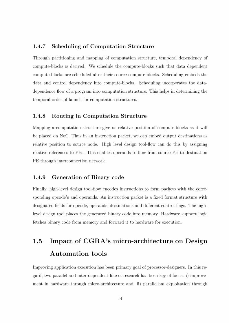
1.4.7 Scheduling of Computation Structure . . . . . . . . . . . . . . . . . 14

1.4.8 Routing in Computation Structure . . . . . . . . . . . . . . . . . . 14

1.4.9 Generation of Binary code . . . . . . . . . . . . . . . . . . . . . . . 14

1.5 Impact of CGRA’s micro-architecture on Design Automation tools . . . . . 14

1.5.1 CGRA with Superscalar PEs . . . . . . . . . . . . . . . . . . . . . 15

1.5.2 CGRA with Multi-threaded PEs . . . . . . . . . . . . . . . . . . . . 17

1.5.3 CGRA with VLIW PEs . . . . . . . . . . . . . . . . . . . . . . . . 17

ix

1.5.4 CGRA with TTA PEs . . . . . . . . . . . . . . . . . . . . . . . . . 18

1.5.5 CGRA with CFUs PEs . . . . . . . . . . . . . . . . . . . . . . . . . 18

1.6 Motivation: Partitioning and Mapping computation structure with respect

to CGRA . . . . . . . . . . . . . . . . . . . . . . . . . . . . . . . . . . . . 19

1.7 Contribution . . . . . . . . . . . . . . . . . . . . . . . . . . . . . . . . . . . 20

1.8 Thesis Organization . . . . . . . . . . . . . . . . . . . . . . . . . . . . . . . 20

2 Partitioning 22

2.1 Background . . . . . . . . . . . . . . . . . . . . . . . . . . . . . . . . . . . 22

2.2 GRAPH . . . . . . . . . . . . . . . . . . . . . . . . . . . . . . . . . . . . . 23

2.2.1 Definitions . . . . . . . . . . . . . . . . . . . . . . . . . . . . . . . . 24

2.2.2 Elements of a Graph . . . . . . . . . . . . . . . . . . . . . . . . . . 26

2.2.3 Graph Representation Data-Structures . . . . . . . . . . . . . . . . 28

2.2.4 Graph Traversal . . . . . . . . . . . . . . . . . . . . . . . . . . . . . 29

2.3 Problem Formulation . . . . . . . . . . . . . . . . . . . . . . . . . . . . . . 31

2.3.1 Problem Analysis and Cost Function . . . . . . . . . . . . . . . . . 31

2.4 Partitioning: A retrospective view . . . . . . . . . . . . . . . . . . . . . . . 32

2.4.1 Random or exhaustive or all combinatorial search . . . . . . . . . . 32

2.4.2 Move based Heuristics . . . . . . . . . . . . . . . . . . . . . . . . . 33

2.4.3 Meta-Heuristics . . . . . . . . . . . . . . . . . . . . . . . . . . . . . 33

2.5 Partitioning: Algorithms, Orthogonal Approaches and Discussion . . . . . 33

2.5.1 Kernighan-Lin (KL) Algorithm . . . . . . . . . . . . . . . . . . . . 33

2.5.2 Greedy Graph Growing Partitioning (GGGP) . . . . . . . . . . . . 34

2.5.3 Two orthogonal approach to partitioning . . . . . . . . . . . . . . . 35

2.5.4 Discussion . . . . . . . . . . . . . . . . . . . . . . . . . . . . . . . . 36

2.6 GoPart : A Cluster-Base Level Partitioning . . . . . . . . . . . . . . . . . 36

2.6.1 Step One: Root Selection . . . . . . . . . . . . . . . . . . . . . . . 39

2.6.2 Step Two: Updating Neighbor-Set and Affinity matrix . . . . . . . 40

2.6.3 Step Three: Iteration . . . . . . . . . . . . . . . . . . . . . . . . . . 40

2.7 Example . . . . . . . . . . . . . . . . . . . . . . . . . . . . . . . . . . . . . 41

x

2.8 Summary of the chapter . . . . . . . . . . . . . . . . . . . . . . . . . . . . 46

3 Mapping 48

3.1 Background . . . . . . . . . . . . . . . . . . . . . . . . . . . . . . . . . . . 49

3.2 Related Work . . . . . . . . . . . . . . . . . . . . . . . . . . . . . . . . . . 50

3.2.1 Dimension reductionist approach . . . . . . . . . . . . . . . . . . . 50

3.2.2 Fix topologies of source and target graph . . . . . . . . . . . . . . . 50

3.2.3 Mapping as a Generic Framework . . . . . . . . . . . . . . . . . . . 50

3.3 Interconnection Network Design Parameters . . . . . . . . . . . . . . . . . 51

3.3.1 Number of Edges in Network . . . . . . . . . . . . . . . . . . . . . 51

3.3.2 Symmetry of Network . . . . . . . . . . . . . . . . . . . . . . . . . 52

3.3.3 Diameter of Network . . . . . . . . . . . . . . . . . . . . . . . . . . 52

3.3.4 Degree of Node . . . . . . . . . . . . . . . . . . . . . . . . . . . . . 53

3.3.5 Bisection Width . . . . . . . . . . . . . . . . . . . . . . . . . . . . . 53

3.3.6 I/O bandwidth . . . . . . . . . . . . . . . . . . . . . . . . . . . . . 53

3.4 Symmetric Interconnection Network (SIN) . . . . . . . . . . . . . . . . . . 54

3.5 Mapping: A Set-Theoretic Foundation . . . . . . . . . . . . . . . . . . . . 55

3.5.1 Function . . . . . . . . . . . . . . . . . . . . . . . . . . . . . . . . . 55

3.5.2 Mapping as a Correspondence function . . . . . . . . . . . . . . . . 57

3.6 Cost Function . . . . . . . . . . . . . . . . . . . . . . . . . . . . . . . . . . 58

3.7 Graph Modelling: Salient features and prospects in Mapping . . . . . . . . 59

3.7.1 Communication Graph (CG) . . . . . . . . . . . . . . . . . . . . . . 59

3.7.2 Isomorphic Graphs . . . . . . . . . . . . . . . . . . . . . . . . . . . 59

3.7.3 Sub-graph Isomorphism . . . . . . . . . . . . . . . . . . . . . . . . 60

3.7.4 Cayley Graph and Cayley Tree . . . . . . . . . . . . . . . . . . . . 61

3.7.5 Discussion . . . . . . . . . . . . . . . . . . . . . . . . . . . . . . . . 63

3.8 The Graph Oriented Mapping Algorithm (GoMap) . . . . . . . . . . . . . 63

3.8.1 First Phase: MAP-Tree Construction . . . . . . . . . . . . . . . . . 64

3.8.2 Second Phase : MAP-Tree Conflict Check and Resolution . . . . . . 65

3.8.3 Final Phase : Resource Matrix Generation and Physical Placement 67

xi

3.9 Summary . . . . . . . . . . . . . . . . . . . . . . . . . . . . . . . . . . . . 68

4 Mapping Case-Study 69

4.1 Symmetric Interconnection Network (SIN): A Revisit . . . . . . . . . . . . 69

4.2 Honeycomb . . . . . . . . . . . . . . . . . . . . . . . . . . . . . . . . . . . 70

4.2.1 Topological Characteristics . . . . . . . . . . . . . . . . . . . . . . . 70

4.2.2 Honeycomb as a Cayley Graph . . . . . . . . . . . . . . . . . . . . 71

4.3 Mapping onto Honeycomb . . . . . . . . . . . . . . . . . . . . . . . . . . . 71

4.3.1 MAP-Tree Construction . . . . . . . . . . . . . . . . . . . . . . . . 72

4.3.2 MAP-Tree Conflict Check and Resolution . . . . . . . . . . . . . . 74

4.3.3 Resource Matrix Generation and Physical Placement . . . . . . . . 75

4.4 Example . . . . . . . . . . . . . . . . . . . . . . . . . . . . . . . . . . . . . 76

4.4.1 MAP-Tree Construction . . . . . . . . . . . . . . . . . . . . . . . . 77

4.4.2 MAP-Tree Conflict Check and Resolution . . . . . . . . . . . . . . 79

4.4.3 Resource Matrix generation and Physical Placement . . . . . . . . 79

4.5 Mesh . . . . . . . . . . . . . . . . . . . . . . . . . . . . . . . . . . . . . . . 79

4.5.1 Topological Characteristics . . . . . . . . . . . . . . . . . . . . . . . 81

4.5.2 Isomorphism between Mesh and Cayley Graph . . . . . . . . . . . . 82

4.6 Mapping onto Mesh . . . . . . . . . . . . . . . . . . . . . . . . . . . . . . . 83

4.6.1 MAP-Tree Construction . . . . . . . . . . . . . . . . . . . . . . . . 83

4.6.2 MAP-Tree Conflict Check and Resolution . . . . . . . . . . . . . . 85

4.6.3 Resource Matrix Generation and Physical Placement . . . . . . . . 85

4.7 Summary . . . . . . . . . . . . . . . . . . . . . . . . . . . . . . . . . . . . 86

5 Results 87

5.1 GoPart Performance . . . . . . . . . . . . . . . . . . . . . . . . . . . . . . 87

5.1.1 Experimental Set-up and Methodology . . . . . . . . . . . . . . . . 88

5.1.2 Results . . . . . . . . . . . . . . . . . . . . . . . . . . . . . . . . . . 89

5.2 GoMap performance . . . . . . . . . . . . . . . . . . . . . . . . . . . . . . 91

5.2.1 Target Topology . . . . . . . . . . . . . . . . . . . . . . . . . . . . 92

xii

5.2.2 Results . . . . . . . . . . . . . . . . . . . . . . . . . . . . . . . . . . 92

5.3 Summary of the chapter . . . . . . . . . . . . . . . . . . . . . . . . . . . . 93

6 Conclusion and Future Work 94

6.1 Conclusion . . . . . . . . . . . . . . . . . . . . . . . . . . . . . . . . . . . . 94

6.2 Future Work . . . . . . . . . . . . . . . . . . . . . . . . . . . . . . . . . . . 96

Bibliography 99

xiii

List of Figures

1.1 A Computing System and a Distributed Computing System . . . . . . . . 2

1.2 Design automation flow for mapping an application on CGRA . . . . . . . 8

1.3 Basic-Block and CFG creation . . . . . . . . . . . . . . . . . . . . . . . . . 9

1.4 key dataflow symbols . . . . . . . . . . . . . . . . . . . . . . . . . . . . . . 11

1.5 CFG and DFG . . . . . . . . . . . . . . . . . . . . . . . . . . . . . . . . . 12

1.6 Hardware software co-space division . . . . . . . . . . . . . . . . . . . . . . 16

2.1 Partitioning of Graph: A Necessity . . . . . . . . . . . . . . . . . . . . . . 23

2.2 A Graph . . . . . . . . . . . . . . . . . . . . . . . . . . . . . . . . . . . . . 24

2.3 A Directed Graph . . . . . . . . . . . . . . . . . . . . . . . . . . . . . . . . 26

2.4 An Example DAG . . . . . . . . . . . . . . . . . . . . . . . . . . . . . . . 39

2.5 Example Graph for Partitioning . . . . . . . . . . . . . . . . . . . . . . . . 41

2.6 Partitioned Groups of Example Graph . . . . . . . . . . . . . . . . . . . . 46

3.1 Mapping of a Computation Structure on a Network Topology . . . . . . . 49

3.2 Example of Interconnection Networks . . . . . . . . . . . . . . . . . . . . . 52

3.3 Examples of Symmetric Interconnection Network (SIN) . . . . . . . . . . . 55

3.4 Different kind of functions . . . . . . . . . . . . . . . . . . . . . . . . . . . 56

3.5 Mapping of CG to RG . . . . . . . . . . . . . . . . . . . . . . . . . . . . . 57

3.6 Source Graph . . . . . . . . . . . . . . . . . . . . . . . . . . . . . . . . . . 60

3.7 Isomorphic Graphs G and G’ . . . . . . . . . . . . . . . . . . . . . . . . . 61

3.8 Cayley Tree (Bethe Lattice) of degree 3 . . . . . . . . . . . . . . . . . . . . 61

3.9 Isomorphism between (unfolded subgraph) SIN and Cayley Tree . . . . . . 62

xiv

3.10 Mapping Framework . . . . . . . . . . . . . . . . . . . . . . . . . . . . . . 64

4.1 Examples of Symmetric Interconnection Network (SIN) . . . . . . . . . . . 70

4.2 Isomorphism between Honeycomb (un-folded) and Cayley Tree . . . . . . . 72

4.3 Cayley Tree Representation from a Cayley Graph (Honeycomb) Prespective 73

4.4 Conflict Scenario . . . . . . . . . . . . . . . . . . . . . . . . . . . . . . . . 73

4.5 Different Conflict Cases of MAP-Tree . . . . . . . . . . . . . . . . . . . . 74

4.6 Conflict Resolution of MAP-Tree . . . . . . . . . . . . . . . . . . . . . . . 75

4.7 Source Graph . . . . . . . . . . . . . . . . . . . . . . . . . . . . . . . . . . 76

4.8 MAP-Tree Construction from Source Graph . . . . . . . . . . . . . . . . . 80

4.9 MAP-Tree with Placing on HoneyComb . . . . . . . . . . . . . . . . . . . 81

4.10 Mesh: an extension of linear-array . . . . . . . . . . . . . . . . . . . . . . . 82

4.11 Cayley Tree (Bethe Lattice) of degree 4 . . . . . . . . . . . . . . . . . . . . 83

4.12 Mesh as Representation of Cayley Tree . . . . . . . . . . . . . . . . . . . . 84

5.1 Algorithms performance on ”delay” to begin of execution of partitions . . . 89

5.2 Algorithms performance with respect to ”communication overhead” across

the partitions . . . . . . . . . . . . . . . . . . . . . . . . . . . . . . . . . . 90

5.3 GoPart execution performance in comparison with Cluster-based Partition-

ing and Level-based Partitioning . . . . . . . . . . . . . . . . . . . . . . . . 90

5.4 GoMap performance with in comparison with Optimal, vis-a-vis on appli-

cation basis . . . . . . . . . . . . . . . . . . . . . . . . . . . . . . . . . . . 91

5.5 Performance With respect to ’Number of Nodes’ of application . . . . . . . 92

6.1 Partitioning and Mapping frame-work . . . . . . . . . . . . . . . . . . . . . 95

xv

List of Tables

2.1 Affinity Matrix . . . . . . . . . . . . . . . . . . . . . . . . . . . . . . . . . 38

4.1 Sorted table of Total Communication For Each Node . . . . . . . . . . . . 77

4.2 Configuration Matrix . . . . . . . . . . . . . . . . . . . . . . . . . . . . . 79

xvi

Chapter 1

Introduction

In this chapter we discuss the role of an automation tool in execution of an application.

Further it puts the work presented in this thesis in context through a discussion on Coarse

Grained Reconfigurable Architecture (CGRA). We detail on computation structures as a

necessary constituent for parallel execution of a program and discuss their mapping onto

CGRA.

1.1 Role of a processor in application development

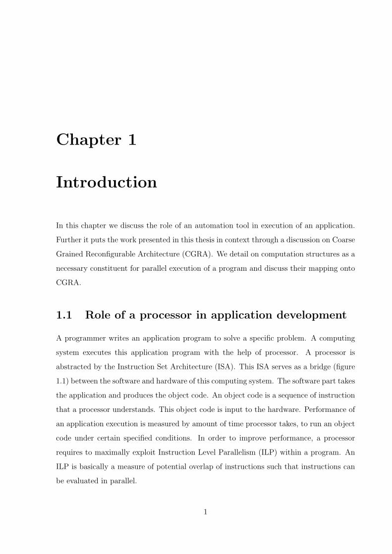
A programmer writes an application program to solve a specific problem. A computing

system executes this application program with the help of processor. A processor is

abstracted by the Instruction Set Architecture (ISA). This ISA serves as a bridge (figure

1.1) between the software and hardware of this computing system. The software part takes

the application and produces the object code. An object code is a sequence of instruction

that a processor understands. This object code is input to the hardware. Performance of

an application execution is measured by amount of time processor takes, to run an object

code under certain specified conditions. In order to improve performance, a processor

requires to maximally exploit Instruction Level Parallelism (ILP) within a program. An

ILP is basically a measure of potential overlap of instructions such that instructions can

be evaluated in parallel.

1

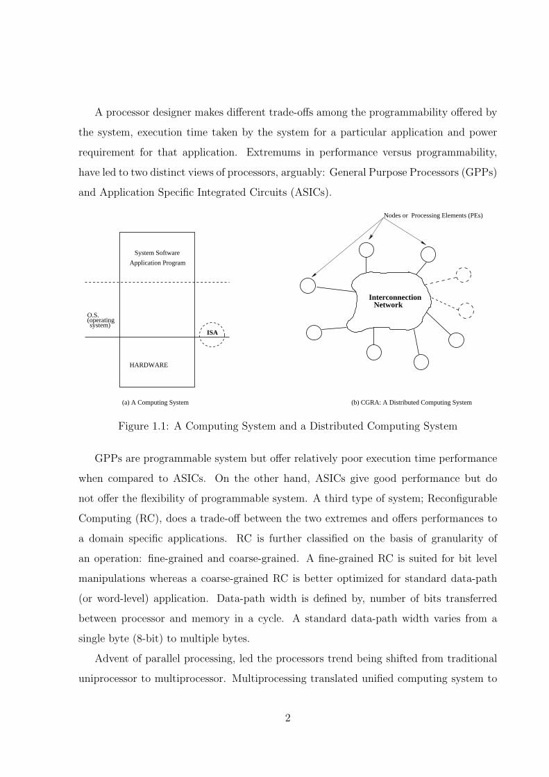
A processor designer makes different trade-offs among the programmability offered by

the system, execution time taken by the system for a particular application and power

requirement for that application. Extremums in performance versus programmability,

have led to two distinct views of processors, arguably: General Purpose Processors (GPPs)

and Application Specific Integrated Circuits (ASICs).

Processing Elements (PEs)

InterconnectionNetwork

O.S.

system)(operating

ISA

HARDWARE

Application Program

System Software

(a) A Computing System (b) CGRA: A Distributed Computing System

Nodes or

Figure 1.1: A Computing System and a Distributed Computing System

GPPs are programmable system but offer relatively poor execution time performance

when compared to ASICs. On the other hand, ASICs give good performance but do

not offer the flexibility of programmable system. A third type of system; Reconfigurable

Computing (RC), does a trade-off between the two extremes and offers performances to

a domain specific applications. RC is further classified on the basis of granularity of

an operation: fine-grained and coarse-grained. A fine-grained RC is suited for bit level

manipulations whereas a coarse-grained RC is better optimized for standard data-path

(or word-level) application. Data-path width is defined by, number of bits transferred

between processor and memory in a cycle. A standard data-path width varies from a

single byte (8-bit) to multiple bytes.

Advent of parallel processing, led the processors trend being shifted from traditional

uniprocessor to multiprocessor. Multiprocessing translated unified computing system to

2

a distributed system. A distributed system is constituted by two features:

i) Presence of multiple autonomous Processing Elements (PEs) or nodes and,

ii) These nodes communicate with each other by message passing.

This array of nodes can execute concurrently in parallel. Nodes in distributed system are

connected with an interconnection network (figure 1.1). Framework of interconnection

network characterizes the coupling among nodes, viz., loosely-coupled and tightly-coupled.

A loosely coupled distributed system employs network topology such as a Local Area

Network (LAN), as it’s interconnection network. A tightly coupled distributed system

uses switched fabric for it’s underlying interconnection network. Switch fabric is a network

topology in which, nodes are connected with each other via network switches. In a tightly

coupled distributed system, PEs are grouped to carry out a specific computation. Switch

fabric based architectures differs from bus based architecture where all nodes share a

common bus.

CGRA are a special case of a tightly coupled distributed system. In this thesis, we

focus on CGRAs where the switched fabric interconnection is a Network-on-Chip (NoC).

This NoC represents the communication sub-system between PEs. CGRAs are better

equipped for high throughput data transport, as communication link are distributed across

multiple physical links. In contrary, bus based systems are based on broadcast data

transmission, that may result in frequent collisions in shared communication medium.

1.2 Design Automation

Program execution can be made faster by effective utilization of hardware resources. This

includes exploiting parallelism from program code, executing independent block of codes

on sufficient hardware resources and finally, aggregating individual computations to get

the end result. This complete process necessitate an automation in order to deal with

a wide range of applications. A design automation tool bridges software and hardware

aspects of program execution. These tools take programmatic representation of an appli-

cation as input and produces binary executable code. This representation is characterized

by the abstraction level of programming language. This classifies design automation tools

3

into two types, viz. low-level and high-level.

Low-level design tools takes an application, represented in low-level languages such

as Hardware Description Languages (HDLs). Instruction set of these languages directly

mimic the hardware. This requires application programmer to have thorough understand-

ing of hardware organization. Thus a programmer undergoes a long learning curve before

he can exploit all the architectural features. This process is further facilitated by a HDL

compiler or assembler.

A high-level design tools takes an application, represented in a High Level Language

(HLL) such as C, C++, Java etc. This led application programmer to focus on algorithm

without worrying about the micro-architectural details involved in program execution.

A good high-level design tool facilitates an automatic exploitation of parallelism that is

inherent in application program. High-level design tool also help processor in assigning

hardware resources such that, resources are judiciously used during program execution.

System softwares that help in this complete process are language compilers, preprocessors,

translators etc.

1.3 Perspectives in Application Execution

We take an application algorithm and discuss the key features that can speed-up the

program execution.

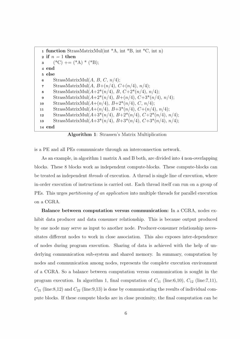
1.3.1 An Example: Strassen’s Matrix Multiplication Algorithm

Strassen’s [2] algorithm uses divide-and-conquer [3] approach for matrix multiplication.

Let A and B be two n× nmatrices, where n is an integer. Partition the two input matrices

A and B into blocks. Multiplication of blocked matrices yield the blocked product matrix

C as follows.

This yield is achieved through intermediate matrices Pk’s, that are defined below:

P1 = (A11 + A22)(B11 + B22)

P2 = (A21 + A22)B11

4

P3 = A11(B12 − B22)

P4 = A22(B21 − B11)

P5 = (A11 + A12)B22

P6 = (A21 − A11)(B11 + B12)

P7 = (A12 − A22)(B21 + B22)

These are further used to express Cij in terms of Pk. Traditional matrix multiplication

takes eight multiplication for this but with help of defined Pk, we can bypass one matrix

multiplication and reduce the number of multiplications to 7 (one multiplication for each

Pk) and express the Cij as:

C11 = P1 + P4 - P5 + P7

C12 = P3 + P5

C21 = P2 + P4

C22 = P1 + P3 - P2 + P6

In algorithm 1 we provide C type pseudo code to accomplish Strassen’s matrix mul-

tiplication. This uses divide-and-conquer approach. This becomes visible in dividing

computation of matrix multiplication into multiple blocks. These blocks can carry out

multiplication independent of each other. This gives the advantage over traditional ma-

trix multiplication which is sequential in nature. Time-bound for Strassen’s algorithm [2]

is O(n2.807) whereas traditional matrix multiplication is O(n3).

1.3.2 Discussion

In order to improve the program execution, the key aspects that should be considered

are:

Exploiting parallelism: Sequential execution of a program only has a single line

of execution. To speed-up execution, a program needs to be driven through parallel

execution of lines. This parallelism is exploited through independent blocks of program

code by a high-level design tool and a CGRA concurrently executes these designated

blocks onto different PEs. Thus in context of CGRAs, concurrency brings the notion of

parallel system. CGRA as a parallel system is represented in figure 1.1 where each node

5

function StrassMatrixMul(int *A, int *B, int *C, int n)1

if n = 1 then2

(*C) += (*A) * (*B);3

end4

else5

StrassMatrixMul(A, B, C, n/4);6

StrassMatrixMul(A, B+(n/4), C+(n/4), n/4);7

StrassMatrixMul(A+2*(n/4), B, C+2*(n/4), n/4);8

StrassMatrixMul(A+2*(n/4), B+(n/4), C+3*(n/4), n/4);9

StrassMatrixMul(A+(n/4), B+2*(n/4), C, n/4);10

StrassMatrixMul(A+(n/4), B+3*(n/4), C+(n/4), n/4);11

StrassMatrixMul(A+3*(n/4), B+2*(n/4), C+2*(n/4), n/4);12

StrassMatrixMul(A+3*(n/4), B+3*(n/4), C+3*(n/4), n/4);13

end14

Algorithm 1: Strassen’s Matrix Multiplication

is a PE and all PEs communicate through an interconnection network.

As an example, in algorithm 1 matrix A and B both, are divided into 4 non-overlapping

blocks. These 8 blocks work as independent compute-blocks. These compute-blocks can

be treated as independent threads of execution. A thread is single line of execution, where

in-order execution of instructions is carried out. Each thread itself can run on a group of

PEs. This urges partitioning of an application into multiple threads for parallel execution

on a CGRA.

Balance between computation versus communication: In a CGRA, nodes ex-

hibit data producer and data consumer relationship. This is because output produced

by one node may serve as input to another node. Producer-consumer relationship neces-

sitates different nodes to work in close association. This also exposes inter-dependence

of nodes during program execution. Sharing of data is achieved with the help of un-

derlying communication sub-system and shared memory. In summary, computation by

nodes and communication among nodes, represents the complete execution environment

of a CGRA. So a balance between computation versus communication is sought in the

program execution. In algorithm 1, final computation of C11 (line:6,10), C12 (line:7,11),

C21 (line:8,12) and C22 (line:9,13) is done by communicating the results of individual com-

pute blocks. If these compute blocks are in close proximity, the final computation can be

6

done faster. This necessitates effective mapping of threads onto PEs of CGRA, such that

closely communicating nodes are together.

In next section we give an overall flow for mapping an application such that the

prospects discussed above are incorporated.

1.4 Mapping an application on CGRA

In this section, we discuss mapping an application since its inception as a high level

language representation till the generation of binary executable code. As described earlier,

we focus on high-level design automation tool for this process. We also give the complete

execution flow that is needed for such tools. Figure 1.2 summarizes necessary steps in a

high level design automation tool-flow for mapping an application on a CGRA. Description

of each step is given below:

1.4.1 Parsing and Intermediate Representation

As mentioned in section 1.2, we begin with specifying an application in a high-level lan-

guage (HLL). Commonly used HLLs are C, Fortran, C++ etc. A HLL uses programming

constructs as abstractions of the computing system. Thus development and maintenance

of a program becomes easier when compared to low-level language implementation. As

a downside, programmers have very little scope to intervene in program execution. A

HLL specification is parsed for syntactical checks using a parser [4]. Parser is a module of

HLL compiler [4,5] that matches every syntax of program specification with the grammar

of the language. Parsed HLL specification is translated into a low-level code representa-

tion. This low-level code is named as Intermediate Representation (IR). Importance of

an IR [6–8] lies in its exposition to finer details. These finer details helps in exploitation

of micro-architectural features of the target platform. IR is treated as a base for all the

future steps of mapping an application. Thus an IR should constitute following features:

i) independence with source language, ii) low-level instruction set, that can be exposed

to bring out finer details of micro-architecture and, iii) independent runtime environment

7

or semantics on program [7].

Target Architecture Independent

Application

Programming Language SpecificationEx. High Level language (HLL) etc

Data Flow Graph (DFG) Creation

Clustering(Computation Structure generation)

Intermediate representation (IR)

3−Address Code etc.Ex. Single Static Assignment (SSA),

OptimizationData and Control Dependency

Binary Files of Computation Structures

Execution Fabric

SOFTWARE

HARDWARE

Support logic

Routing

Scheduling Cluster

Mapping Clusters

Partitioning Clusters

Code Generation

Target Architecture Dependent

Figure 1.2: Design automation flow for mapping an application on CGRA

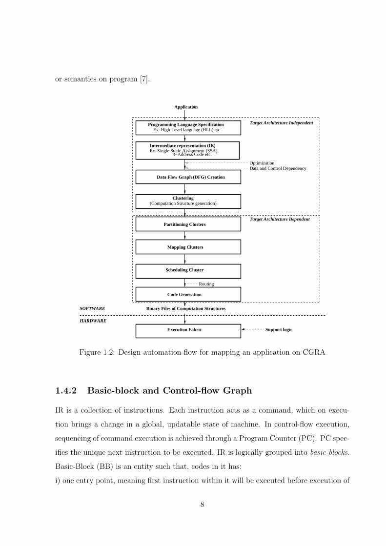
1.4.2 Basic-block and Control-flow Graph

IR is a collection of instructions. Each instruction acts as a command, which on execu-

tion brings a change in a global, updatable state of machine. In control-flow execution,

sequencing of command execution is achieved through a Program Counter (PC). PC spec-

ifies the unique next instruction to be executed. IR is logically grouped into basic-blocks.

Basic-Block (BB) is an entity such that, codes in it has:

i) one entry point, meaning first instruction within it will be executed before execution of

8

any other instruction in it.

ii) one exit point, meaning only the last instruction transfers the flow of execution to a

different basic block.

Sequential execution of a program moves from one basic-block to another basic-block. Ex-

ecuting basic-block gives an atomic flow of program execution i.e. either a basic-block is

executed completely or none of it’s instruction gets executed. This mimics the control-flow

of execution with basic-blocks as elementary building blocks of the program.

Control-flow of program execution is represented through Control Flow Graph (CFG).

A CFG is a graph whose nodes are basic-blocks and the edges represents control-flow.

Thus an edge from node A to node B in CFG, indicates that execution of node A may be

followed immediately by execution of node B. A basic-block is uniquely labeled as “start”

which has no incoming edges and a basic-block is uniquely labeled as “end” which has no

outgoing edges. All edges in a CFG are assumed to exist between start basic-block and

end basic-block. Start basic-block and end basic-block together constitutes the notion of

fork and join in a CFG.

A CFG is a graphical representation of all possible paths that might be traversed

through a program during it’s execution. A typical example of CFG formation for a piece

of code is illustrated in figure 1.3. This code-fragment represents a program, that com-

pares between summation (x) and multiplication (y), of two numbers a and b. In figure

BB2

7: L1: end program

2: y:= a*b3: if x > y4: x:= x+15: goto L1

1: x:= a+b1: x:= a+b2: y:= a*b3: if x > y

BB4

BB1

7: L1: end program6: y:=y+1

BB1

BB2

BB3

BB4

(a) fragment of code/ illustration of basic−blocks (b) CFG

6: y:=y+1

BB3

4: x:= x+15: goto L1

Figure 1.3: Basic-Block and CFG creation

1.3(a), there are 4 basic-blocks: BB1 from line 0 to 1, BB2 from line 3 to 5, BB3 at line

9

6 and BB4 at line 7. Here BB1 is the “entry block” and BB4, the “exit block”. A CFG

generated from this is shown in figure 1.3(b).

1.4.3 Data-flow Graph (DFG) construction

A computing system follows either control-flow execution or data-flow execution. A data-

flow execution means that an operation is ready to execute as soon as it’s operands are

available. This is in contrast with control-flow of execution which is governed by a pro-

gram counter. Thus a data-driven execution gives ample scope for exploiting parallelism.

CGRAs being a distributed system, facilitates data-driven execution as this enables to

expose CGRA’s PEs for parallel execution.

A control-flow execution has it’s foundation in a CFG, similarly a data-flow execution

has it’s foundation in a Data Flow Graph (DFG). A DFG [9] is a graphical representation

of all the data-dependencies, that may incur in program execution. The nodes in the DFG

represent the operation that are to be performed and the edges of the DFG represent the

transports. Below we give the DFG definition and it’s semantics for execution.

DFG Definition: A DFG G(V,E) is defined such that,

Nodes (V ): have input/output data ports and,

Edges (E): connects output ports and input ports.

DFG Execution Semantics:

- Ready to fire the operation as soon as input data are ready. This is subjected to

availability of functional units (FU’s) or logic units (LU’s), in case of multiple “ready to

fire” operations.

- Consumes data from input ports and produce data to its output ports.

There may be many nodes at a given time that become as ready to fire.

A DFG is constructed through data-flow analysis of program dependence. Data-flow

analysis derives information about the dynamic behavior of a program by only examining

the static code. In data-flow analysis one gathers the possible set of values at various

points of a program. Data-flow analysis collects information about the way the variable

10

are used, defined in the program. Control statements of CFG help in determining these

values as CFG includes all possible flows. For convenience one can have this information

at basic-block boundaries since from that it is easy to compute the information at points

within the basic block. We consider following three types of statements of a CFG and

establish the corresponding DFG [10]. These statements are:

a) assignments of the form variable := expression,

b) forks as established through a conditional statements like if-else, do-while constructs,

etc. and

c) labeled joins which represent no computation, but are the only nodes in the graph

which can be the target of goto statements.

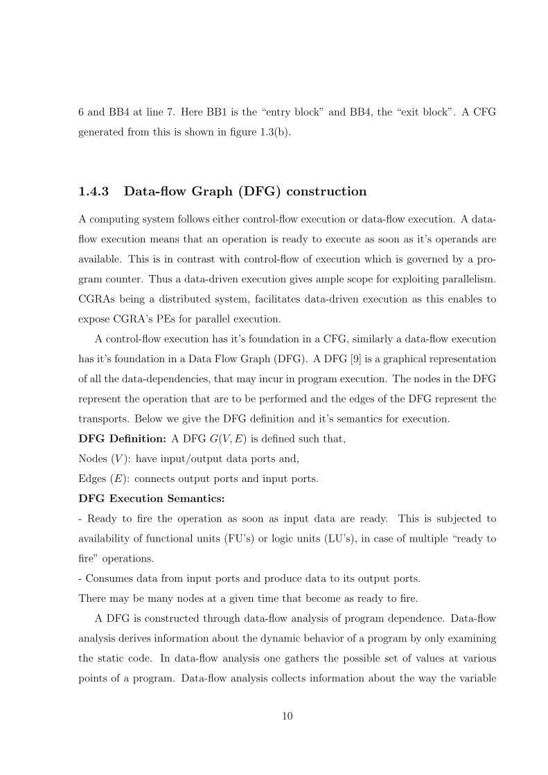
Three important notations switch, merge and synch as shown in figure 1.4, are used as

data-flow operators to represent the transformation of CFG to DFG. Switch is defined as

an operation that takes two inputs x and y, and produces two outputs ztrue and zfalse.

Here x is token-to-carry-forward whereas y is a boolean variable to control forwarding of

the token to ztrue or zfalse. If y is true then, token on x is carried to ztrue otherwise token

is carried to zfalse. Merge is defined as an operation such that it takes inputs x1, x2, . . .

and produces outputs z. A token arriving on an input is output on z. A synch tree is n

inputs, single output i.e. once a token has arrived on each of n input, an output token is

generated.

..

switch

Switch

y

z

Synch

ztrue false

x

X

Merge

z

x1 x2 x1 xi

Figure 1.4: key dataflow symbols

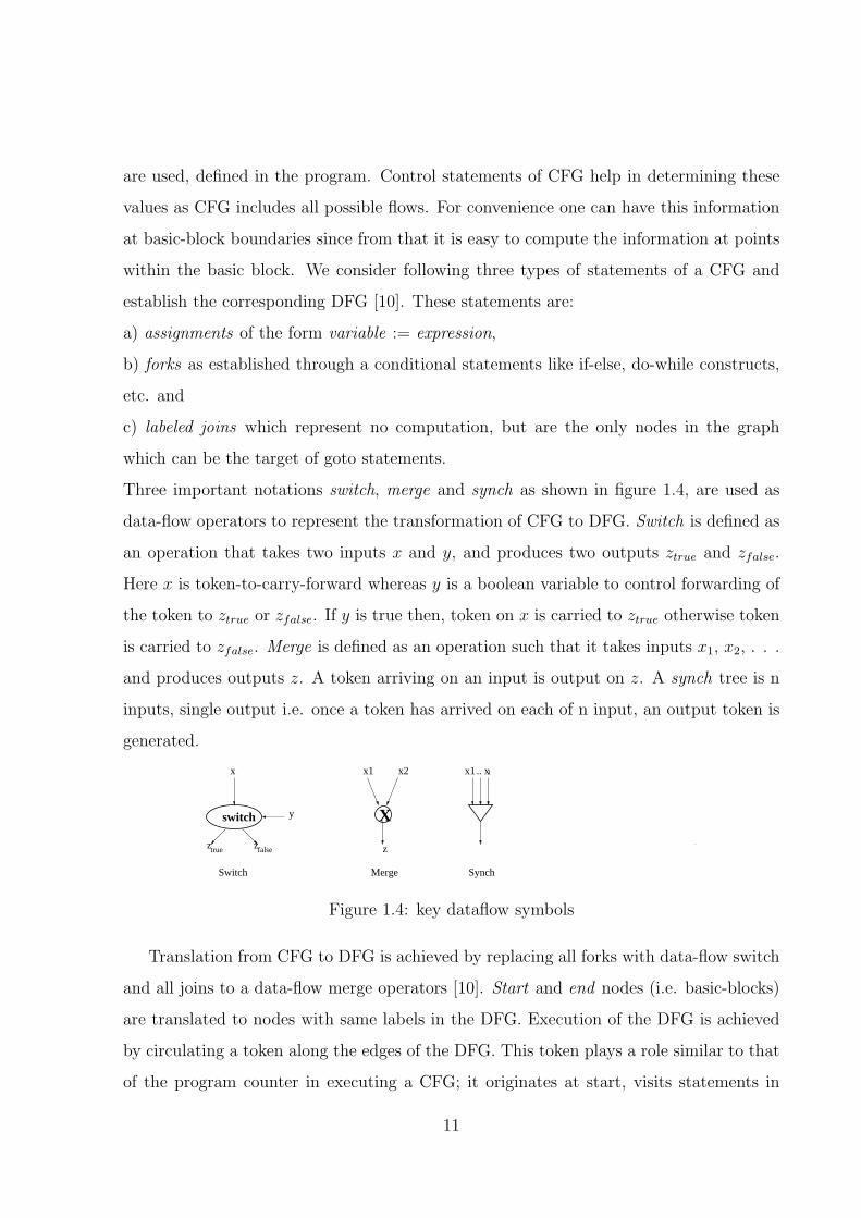
Translation from CFG to DFG is achieved by replacing all forks with data-flow switch

and all joins to a data-flow merge operators [10]. Start and end nodes (i.e. basic-blocks)

are translated to nodes with same labels in the DFG. Execution of the DFG is achieved

by circulating a token along the edges of the DFG. This token plays a role similar to that

of the program counter in executing a CFG; it originates at start, visits statements in

11

sequence, and visits every memory operation within a statement in sequence. Conditional

branching in the CFG is translated through a switch operator that directs the token to one

of two possible destinations. Note that token does not carry any value since it represents

permission to access the stored state of the program variables and hence this is also called

as access token.

An example, CFG to DFG conversion is shown in figure 1.5.

store y

1: x:= a+b2: y:= a*b3: if x > y

BB4

BB1

6: y:=y+1

BB3

4: x:= x+15: goto L1

BB2

7: L1: end program

(a) control−flow graph

load y

>

switch

+1

store x

X

end

+1

load x

t f

(b) data−flow graph

BB2 BB3

BB4

BB1 load a load b

*+

store x store y

load x load y

Figure 1.5: CFG and DFG

1.4.4 Formation of Computation Structure

A DFG represents the complete program. To exploit parallelism we need to segregate

instructions/basic-blocks in different threads such that each thread can be executed in-

dependently. We select basic-blocks in such a fashion that closely communicating basic

blocks are kept together in a thread. Thus a thread, groups the basic blocks. This process

translates to clustering of DFG. Each cluster is referred to as “computation structure”.

12

We achieve coarse-grain parallelism with the help of computation structure. This due to

fact that granularity of execution is at basic-block level.

A computation structure H(V , E) is a subgraph of DFG of the application G(V,E),

where V , V ’ represents vertex sets of application DFG G and computation-structure

H respectively and E, E’ are the edge sets of DFG G and computation-structure H

respectively such that H ⊂ G.

1.4.5 Partitioning of Computation Structure

A computation structure is a collection of several low-level instructions. A CGRA, exe-

cutes these instructions with the help of PEs. A PE has fixed amount of memory that

may not suffice to accommodate all the instructions of a computation structure. This

necessitates partitioning of computation structures. We partition computation structures

such that each partition has number of instruction no more than that of maximum avail-

able slots in each PE. Each part of computation structure is referred as a compute-block.

A compute-block gets executed by one PE.

1.4.6 Mapping of Computation Structure

A partitioned computation structure is represented as an interconnection of compute-

blocks. This is referred as communication graph (CG). A CG is a weighted graph, where a

node represents a compute-block and an edge represents the data dependency between the

compute blocks. Number of data dependencies between two compute-blocks is represented

by weight of edge, that connects them. In hardware, a group of PEs executes one CG.

We aim to place the CG on a set of PEs. The interconnection topology of the PE is

also called as resource graph (RG). The structure of a RG could be different from the

structure of the CG.

In such scenario, we need a mapping procedure to transform the CG (i.e. a source

graph) to fit into RG (i.e. a destination graph). This is done with constraint of one-to-one

mapping of compute-block to PE i.e. one compute-block gets mapped on one PE.

13

1.4.7 Scheduling of Computation Structure

Through partitioning and mapping of computation structure, temporal dependency of

compute-blocks is derived. We schedule the compute-blocks such that data dependent

compute-blocks are scheduled after their source compute-blocks. Scheduling embeds the

data and control dependency into compute-blocks. Scheduling incorporates the data-

dependence flow of a program into computation structure. This helps in determining the

temporal order of launch for computation structures.

1.4.8 Routing in Computation Structure

Mapping a computation structure give us relative position of compute-blocks as it will

be placed on NoC. Thus in an instruction packet, we can embed output destinations as

relative position to source node. High level design tool-flow can do this by assigning

relative references to PEs. This enables operands to flow from source PE to destination

PE through interconnection network.

1.4.9 Generation of Binary code

Finally, high-level design tool-flow encodes instructions to form packets with the corre-

sponding opcode’s and operands. An instruction packet is a fixed format structure with

designated fields for opcode, operands, destinations and different control-flags. The high-

level design tool places the generated binary code into memory. Hardware support logic

fetches binary code from memory and forward it to hardware for execution.

1.5 Impact of CGRA’s micro-architecture on Design

Automation tools

Improving application execution has been primary goal of processor-designers. In this re-

gard, two parallel and inter-dependent line of research has been key of focus: i) improve-

ment in hardware through micro-architecture and, ii) parallelism exploitation through

14

software. These two needs to go hand in hand otherwise gains made by one may be

counteracted by other.

In pursuit of faster execution and hence in exploiting parallelism, architectures have

evolved from uniprocessor specifics to multiprocessor structures. This changed the notion

of program execution from unified computing to distributed computing. Thus bringing

the functionality of CGRA as a distributed computing system. This distribution becomes

apparent with the PEs present in NoC of a CGRA. NoC represents the communication

sub-system between PEs. Thus network topology of interconnection network plays an im-

portant role in flow of information between PEs. Depending on the execution paradigm

of the CGRA, each PE is designed as a processor of a specific architecture viz. super-

scalar [11], multi-threaded, Very Large Instruction Word (VLIW), Transport Triggered

Architecture (TTA) [12], Custom Function Units (CFUs) etc.

In this section, we discuss mapping of an application on a CGRA, with respect to figure

1.2. We evolute this as a separation of responsibilities in the context of software-hardware

space co-division. As discussed in section 1.4, these responsibilities primarily includes:

partitioning of computation structure, mapping of computation structure, scheduling of

computation structure, routing (or data-communication) among computation structures,

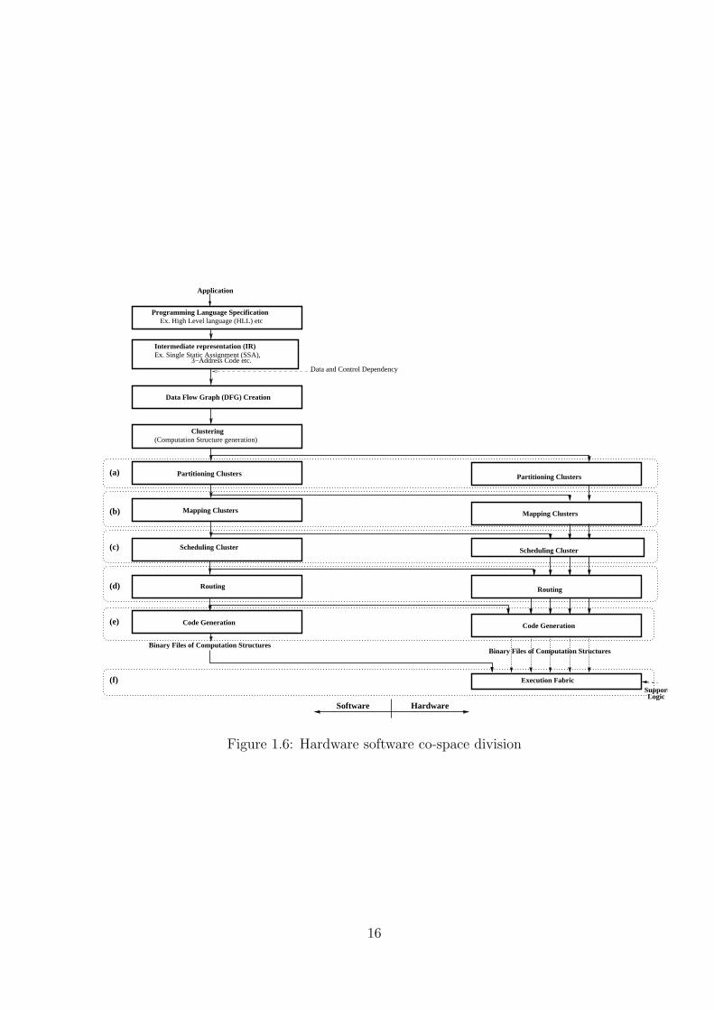
binary code-generation and execution. This is represented as (a), (b), (c), (d), (e) and (f)

in figure 1.6. We can easily conclude that executable binary files (object code) are always

generated by software and execution is always done by hardware. For remaining i.e (a),

(b), (c) and (d), we qualitatively analyse each one as per the computation specifics of PEs

as follows.

1.5.1 CGRA with Superscalar PEs

In superscalars [11], hardware is not very much exposed to compiler. A computation

structure (clustered DFG), is passed to each superscalar node such that each node has

one stream of instructions. This does not involve partitioning of computation structure.

Once the execution of current instruction is done, another instruction from instruction

stream is supplied to PE. Mapping is done by automation tool for each computation

15

(f)

Software Hardware

Application

Programming Language SpecificationEx. High Level language (HLL) etc

Data Flow Graph (DFG) Creation

Clustering(Computation Structure generation)

Intermediate representation (IR)

3−Address Code etc.Ex. Single Static Assignment (SSA),

Scheduling Cluster

Mapping Clusters

Partitioning Clusters

Data and Control Dependency

Scheduling Cluster

Mapping Clusters

Partitioning Clusters

Binary Files of Computation Structures

Code Generation Code Generation

Routing Routing

Execution Fabric

Binary Files of Computation Structures

LogicSupport

(a)

(b)

(c)

(d)

(e)

Figure 1.6: Hardware software co-space division

16

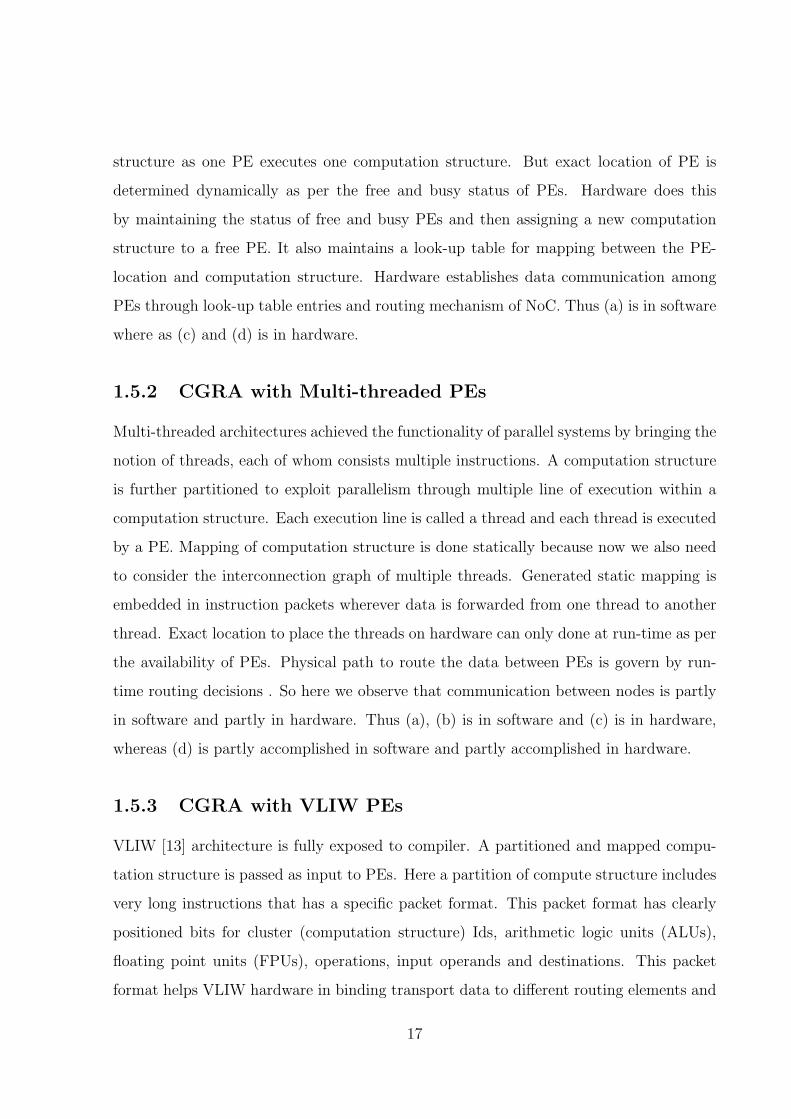
structure as one PE executes one computation structure. But exact location of PE is

determined dynamically as per the free and busy status of PEs. Hardware does this

by maintaining the status of free and busy PEs and then assigning a new computation

structure to a free PE. It also maintains a look-up table for mapping between the PE-

location and computation structure. Hardware establishes data communication among

PEs through look-up table entries and routing mechanism of NoC. Thus (a) is in software

where as (c) and (d) is in hardware.

1.5.2 CGRA with Multi-threaded PEs

Multi-threaded architectures achieved the functionality of parallel systems by bringing the

notion of threads, each of whom consists multiple instructions. A computation structure

is further partitioned to exploit parallelism through multiple line of execution within a

computation structure. Each execution line is called a thread and each thread is executed

by a PE. Mapping of computation structure is done statically because now we also need

to consider the interconnection graph of multiple threads. Generated static mapping is

embedded in instruction packets wherever data is forwarded from one thread to another

thread. Exact location to place the threads on hardware can only done at run-time as per

the availability of PEs. Physical path to route the data between PEs is govern by run-

time routing decisions . So here we observe that communication between nodes is partly

in software and partly in hardware. Thus (a), (b) is in software and (c) is in hardware,

whereas (d) is partly accomplished in software and partly accomplished in hardware.

1.5.3 CGRA with VLIW PEs

VLIW [13] architecture is fully exposed to compiler. A partitioned and mapped compu-

tation structure is passed as input to PEs. Here a partition of compute structure includes

very long instructions that has a specific packet format. This packet format has clearly

positioned bits for cluster (computation structure) Ids, arithmetic logic units (ALUs),

floating point units (FPUs), operations, input operands and destinations. This packet

format helps VLIW hardware in binding transport data to different routing elements and

17

later, in executing the operations and transporting the data. Thus (a), (b) and (c) is in

software and only (d) is in hardware.

1.5.4 CGRA with TTA PEs

TTAs [14] alike VLIW architectures, are fully exposed to compiler. TTAs offer better

compiler control mechanism in comparison to VLIW, as now compiler is also aware of

communication interconnect along with the availability of transport channels (i.e com-

munication ports in network switch). This leads to fewer constraints on scheduling of

data transports. Computation structures are mapped onto group of PEs. Data transport

information is also provided along with computation structures. This led to an effec-

tive routing mechanism for communication between PEs. Thus all (a), (b) and (c) is in

software whereas (d) is primarily accomplished in software and only actual data-transfer

takes place in hardware.

1.5.5 CGRA with CFUs PEs

CFUs are domain specific PEs that are customized to suit a range of application. A

CGRA, with the help of additional support logic, execute operation on these PEs. Since

CFUs are designed with specific computation (and memory) needs, an additional control

logic is needed to support the execution. This functionality is given the name support

logic. CFUs, designed with specific memory bandwidth may trigger the partitioning

of computation structure to suit the memory constraint. Computation structures are

mapped onto PEs with the help of support logic. Routing decision are made at run time

through routing mechanism of NoC.

From above discussion we can safely conclude that partitioning (a) and mapping (b)

phase of computation structure is done statically (by software) and thus highly dependent

on high-level design automation tool. This characterizes the design of automation tools.

18

1.6 Motivation: Partitioning and Mapping computa-

tion structure with respect to CGRA

Partitioning and mapping of computation structures on CGRA hardware is constrained

by the micro-architectural features. While mapping a compute structure there could be a

case that number of instructions in a compute structure exceeds the memory bandwidth

of a PE. In that case, we require to partition computation structure into smaller chunks

such that, each part can be executed on individual node. Each partition of a computation

structure is referred as a compute-block. This gives an interconnection of partitioned

compute structure. This interconnection is mapped as per the structural constraint of

underlying topology of NoC. This topology could be mesh, honeycomb, hypercube etc. ln

chapter 3, we will see that mapping a computation structure is a sub-graph homomorphism

problem as we have two graphs; one as interconnection of compute structure and the other

as the hardware topology and we morph first graph onto the second graph. Here it should

be noted that partitioning of computation structures is a balanced graph-partitioning

problem and is NP-complete [15]. Also, mapping a computation structure is a sub-graph

homomorphism problem and hence NP-complete [15].

Another important aspect of partitioning and mapping of computation structures on

CGRA hardware is, structural and functional variety among nodes in CGRA. Nodes

in CGRA can be of two types: homogeneous and heterogeneous. If all nodes posses

same structure and equal execution capability, then nodes are homogeneous. If nodes are

designed with different structural and computing capability, then nodes are heterogeneous.

Motivation of this thesis is to find an effective, partitioning and mapping of compu-

tation structure onto a homogeneous CGRA such that, an application gets executed in

optimal or near-optimal execution time.

19

1.7 Contribution

This thesis concentrates on: i) partitioning of a computation structure into smaller sub-

structures (compute-blocks), such that each substructure can be executed on individual

PE and then, ii) mapping of a computation structure onto target architecture.

The contribution of this thesis can be summarized as follows:

1. Partition of Computation Structure: This basically constitutes what instruc-

tions should be clubbed together in one compute-block, so that there is optimality

in compute and transport metadata for a computation structure while consider

schedule for compute-blocks. The purpose of computation structure formation is to

exploit the maximum parallelism.

2. Mapping of Computation Structure: The interconnection of nodes on Network-

On-Chip (NoC) is determined by underlined topology. In order to map the com-

putation structure on the target topology, we may require to change the transport

metadata of previously formed computation structure to match the topology. This

phase maps the computation structure under topological constraint of NoC. We do

this in two steps: i) we transform the graph representation of a computation struc-

ture into an intermediate “target-like” graph and then, ii) we map this transformed

graph on target graph.

1.8 Thesis Organization

The rest of thesis is organized as follows:

Chapter 2 presents the computation structure formation. This means partitioning

of an instruction sequence which is represented as a directed acyclic graph (dag).

Chapter 3 presents the mapping of a computation structure on the target architec-

ture. We do this as two step process: In first step, we transform the interconnection of

computation structure into an intermediate graph which is a look-alike graph to desti-

nation graph and then as second step, we map this intermediate graph onto destination

20

graph.

Chapter 4 presents case studies of mapping computation structure on: a) honeycomb

and, b) mesh topology. Here we elaborate the mapping procedure as discussed in chapter

3, with specific examples.

Chapter 5 presents the results of our work. This is done separately with respect to

partitioning and mapping.

Chapter 6 concludes the thesis with the scope of future work.

21

Chapter 2

Partitioning

In this chapter we formulate a partitioning technique for computation structures. This is

discussed with the balance between computation versus communication as the partitioning

objective. We use graph notions and terminologies in association with our partition

technique.

This chapter is organized as follows. In section 2.1 we brief about the necessity of par-

titioning a computation structure. Section 2.2 introduces the basic graph notations and

definitions. In section 2.3, we concentrate on partition problem formulation and assump-

tion model for directed graph. Section 2.4 discusses some existing approaches. Section 2.6

presents our graph partitioning approach. We illustrate graph partition algorithm with

an example in section 2.7.

2.1 Background

In section 1.4 we discussed that in a CGRA, computation structures are identified at com-

pile time in terms of compute metadata and their inter-communication. A computation

structure is a Directed Acyclic Graph (DAG). A DAG representation of computation

structure eases the processing and optimization [4, 5]. A computation structure gets ex-

ecuted on one or more PE. Multiple PEs are used if the number of instructions in a

computation structure exceeds the storage capacity of a PE. In such a case, computation

22

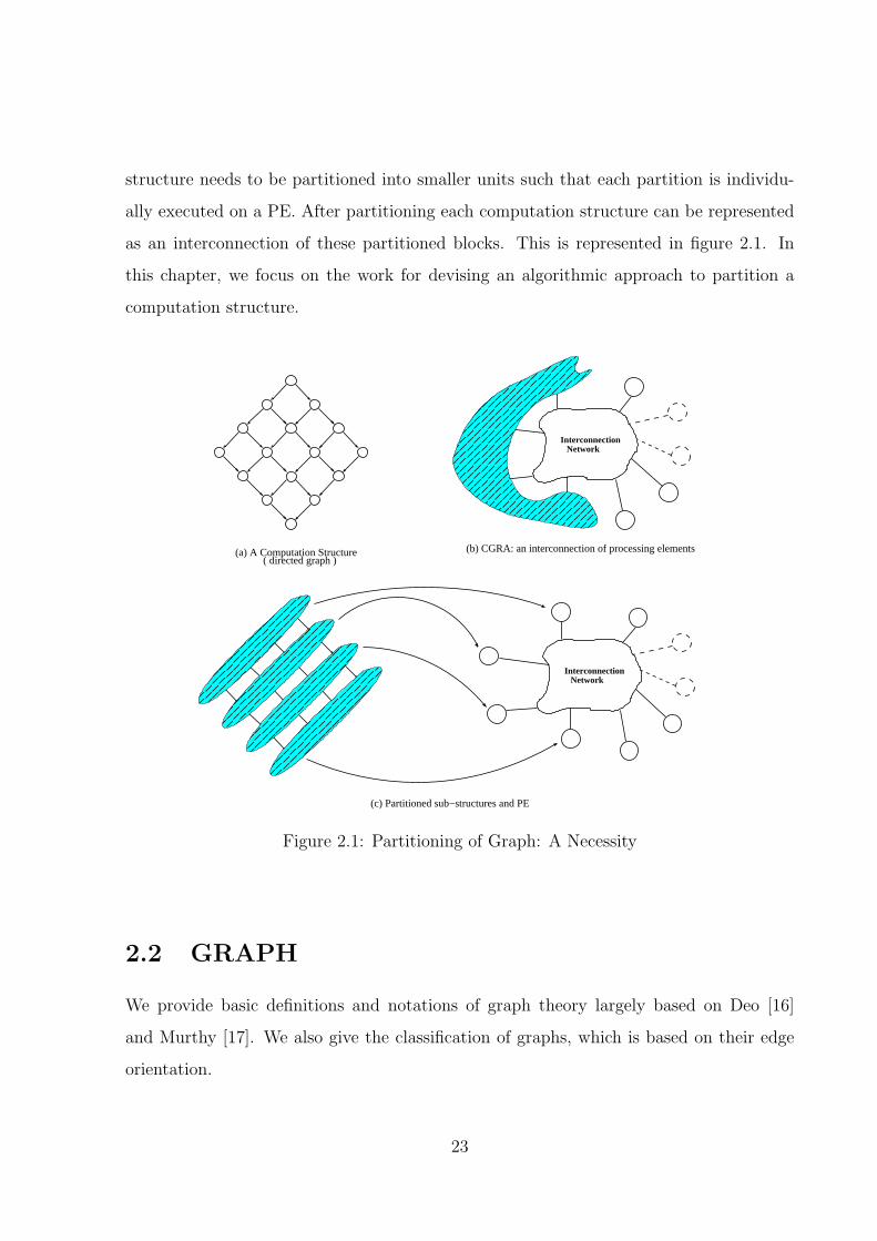
structure needs to be partitioned into smaller units such that each partition is individu-

ally executed on a PE. After partitioning each computation structure can be represented

as an interconnection of these partitioned blocks. This is represented in figure 2.1. In

this chapter, we focus on the work for devising an algorithmic approach to partition a

computation structure.

(a) A Computation Structure( directed graph )

InterconnectionNetwork

InterconnectionNetwork

(c) Partitioned sub−structures and PE

(b) CGRA: an interconnection of processing elements

Figure 2.1: Partitioning of Graph: A Necessity

2.2 GRAPH

We provide basic definitions and notations of graph theory largely based on Deo [16]

and Murthy [17]. We also give the classification of graphs, which is based on their edge

orientation.

23

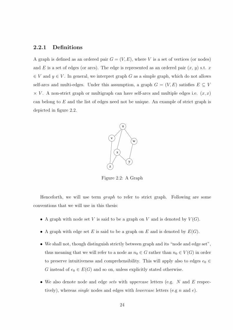
2.2.1 Definitions

A graph is defined as an ordered pair G = (V,E), where V is a set of vertices (or nodes)

and E is a set of edges (or arcs). The edge is represented as an ordered pair (x, y) s.t. x

∈ V and y ∈ V . In general, we interpret graph G as a simple graph, which do not allows

self-arcs and multi-edges. Under this assumption, a graph G = (V,E) satisfies E ⊆ V

× V . A non-strict graph or multigraph can have self-arcs and multiple edges i.e. (x, x)

can belong to E and the list of edges need not be unique. An example of strict graph is

depicted in figure 2.2.

w

u

v

x

zy

Figure 2.2: A Graph

Henceforth, we will use term graph to refer to strict graph. Following are some

conventions that we will use in this thesis:

• A graph with node set V is said to be a graph on V and is denoted by V (G).

• A graph with edge set E is said to be a graph on E and is denoted by E(G).

• We shall not, though distinguish strictly between graph and its “node and edge set”,

thus meaning that we will refer to a node as n0 ∈ G rather than n0 ∈ V (G) in order

to preserve intuitiveness and comprehensibility. This will apply also to edges e0 ∈G instead of e0 ∈ E(G) and so on, unless explicitly stated otherwise.

• We also denote node and edge sets with uppercase letters (e.g. N and E respec-

tively), whereas single nodes and edges with lowercase letters (e.g n and e).

24

Subgraph: Consider a graph G := G(V , E). A graph G′ := G′(V ′, E ′) is called a

subgraph of G, if the vertices and edges of G′ are contained in the vertices and edges of

G i.e. V ′ ⊂ V and E ′ ⊂ E. We can say that,

i) Subgraph G′(V ′, E ′) of G(V , E) is a subgraph induced by its vertices V ′, if its edge set

E ′ contains all edges in G whose end point belong to vertices in G′.

ii) If u is a vertex in G then G-u is the subgraph G′ of graph G obtained by removing u

from G and removing all the edges in G which contain u.

ii) if e is an edge in G then G-e is the subgraph G′ of graph G obtained by removal of

edge e from G.

A subgraph G′ is a graph whose vertices and edges are subsets of the vertices and edges

of a given graph G.

Classification of Graphs:

Graphs can be classified into the following:

Undirected Graph: A graph in which edges do not have any orientation, is known as

undirected graph. This means referring to vertices x and y, an edge e such that, e = {x,y} is not governed by ordered pair relationship and hence can be equivalently expressed

as e = {y, x}. Figure 2.2 is an example of undirected graph.

Directed Graph: A graph in which an edge has an orientation with respect to nodes

is known as directed graph. In these graphs, an edge originates from a source node and

terminates at the destination node. Source node is referred as a head and destination

node as tail of aforesaid edge. An example directed graph is depicted in figure 2.3.

In a directed graph G, let an edge be e= {x, y}, then this edge is said to be directed

from x to y. Here x is called the head and y is called the tail of the edge e.

As we will be using directed graphs for the rest of the document, we adopt the notation

of e = {x → y} or simply {x, y}, which implies the direction of the edge. We will also

refer to nodes of directed graph as source and destination.

25

w

u

v

x

zy

Figure 2.3: A Directed Graph

2.2.2 Elements of a Graph

Adjacent: Two vertices are said to be adjacent if they are joined by an edge. Taking

example of an edge (u, v), vertex u is adjacent to vertex v and vertex v is adjacent to

vertex u. This relationship is used in building of an adjacency matrix or an adjacency

list, which is helpful in representation of a graph.

Degree of a Vertex: Degree of a vertex is defined as the number of neighbours. A

vertex x is said to be a neighbour to another vertex y, if they are adjacent to each other.

The set of neighbours of a vertex in G is denoted by NG(v) or N(v). So degree d(v) of a

vertex v is the number of edges at v.

i.e. d(v) := |N(v)|Here we associate the minimum degree of a graph G as the lowest value of degree among

all its nodes i.e.

δ(G) := min{d(v)|v ∈ V }Similarly, maximum degree of a graph G is the highest value of degree among all its nodes

∆(G) := max{d(v)|v ∈ V }In figure 2.2, d(u) = 3, d(y) = 2 .

Uniformity of degree among all its nodes of a graph, plays a very important role in

determining the characteristics of a graph as regular graph and irregular graph.

Regular Graph: If all the vertices in a graph have the same degree then that graph is

a regular graph. More precisely, if the degree of all the nodes in a graph is k then the

26

graph is said to k-regular. For Example, later in this thesis, we will see that mesh [18] is

a 4-regular graph and honeycomb [19] is a 3-regular graph. Regular graphs have great

advantages over non-regular graphs in many respect. Any algorithmic approach for solving

a problem in such graph, uniformly applies to the whole graph. This obviates the need for

designing a vertex-centric algorithm. Regular graphs can be concisely represented using

group theoretic notations which makes it easy to apply various group theoretic operations

on a regular graph.

Successor and Predecessor: In context of a directed graph two important notations

with respect to nodes are successor and predecessor. This is classified on the precedence

order between two nodes, in which one precedes the another. If a source node is directly

connected (i.e. there exists an edge) to a destination node, then the source node is said

to be direct (or immediate) successor of the destination node and destination node is

said to be a direct (or immediate) predecessor of source node. If a source node is not

connected immediately to a destination node but is connected through a path (i.e. a

sequence of vertices such that from each of its vertices there is an edge to the next vertex

in the sequence), then the source node is said to be successor of the destination node and

destination node is said to be a predecessor of source node. Successors and predecessors

are important notion for information flow within a graph, as they precisely depict the

information about source and sink nodes in a particular communication.

For example in figure 2.3, u is immediate successor of v and v is immediate predecessor

to u. Also, there exists a path between u and x, which puts u as a successor to x and x

as a predecessor to u.

Cycle: In a graph, if a path traverses v0..vk−1 and k ≥ 3 then the graph C := v0..vk−1 +

vk−1v0 is called a cycle.

Directed Acyclic Graph (DAG): Directed acyclic graph is a directed graph with no

directed cycles. It is defined in such a way that there exists, no sequence of vertices

through a path, which eventually leads to a loop.

27

Terminology for Directed Graph with a designated “root”:

Root: A source node which is considered as the first node to begin.

Depth or Level: Level or depth of a node u in rooted digraph is defined as it’s distance

from the root. This numerically equals to the number of edges in the unique directed

path from root to node u. Root is at level (or depth) 0.

Height: Maximum depth among all the nodes is known as height of directed graph.

Parent and Child: If there exists an edge (u, v) such that the direction is from vertex

u to vertex v, then u is parent of v and v is the child of u. Parent and child notation is

interchangeably used with immediate successor and immediate predecessor respectively.

Sibling: Nodes which have same parent are known as siblings.

Leaf: A node without any successor.

Internal Vertex: All non-leaf nodes are known as internal vertexes.

Cut: When we partition a vertex set V of graph G in two disjoint sets, then this is known

as a cut.

Cut-set: A cut-set is, set of all edges whose source and destination vertex lies in two

different sets.

2.2.3 Graph Representation Data-Structures

There are different possible representations of a graph, such as adjacency matrix, adja-

cency list or incidence matrix. Any of these can be used as computer representation of

computation structure i.e a DAG. We, in this thesis, we will be using adjacency matrix

and adjacency list representation. Now there are distinct notions of adjacency matrix for

undirected and directed graph. In an undirected graph we prefer to represent an edge

as both (x, y) and (y, x). This renders the matrix symmetric. In case of directed graph,

adjacency is noted only along the direction of edge. Adjacency list is a list representa-

tion of adjacency’s. Computation structures are usually very sparse, so adjacency list is

space-efficient representation with respect to adjacency matrix.

28

2.2.4 Graph Traversal

Given a graph G = (V , E) and a distinguished root (or source) vertex s, graph traversal

algorithm traverses all the vertices of the graph that are reachable from the root node

s. In general, if a directed graph, does not posses any root node, we designate a root

vertex (preferably one with no incoming edge) as the source node to begin the traversal.

The two important graph traversal algorithms are Breadth First Search (BFS) and Depth

First Search (DFS).

Breadth First Traversal

This is a level wise traversal algorithm where we start from nodes of one level and once

all the nodes at that level are traversed, then we move to next level. This is named

so, because it expands the frontier between discovered and undiscovered nodes uniformly

across the breadth.

The algorithm starts by treating all the vertices of the graph as unmarked. A source

vertex s is marked as visited. We visit every unmarked neighbour ui of s and mark each

ui as visited. Once all unmarked ui are marked as visited, we mark s as finished. This is

repeated on each vertex marked as visited in the order they were visited. Breadth first

search constructs a breadth-first tree with source vertex s as its root. BFS is of our special

concern as we use this for levelling of nodes, which is an initial step in GoPart algorithm

as explained in section 2.6. Psuedo Code for BFS is in algorithm 2.

Depth First Traversal

DFS searches deeper in the graph whenever possible. Starting for s, we visit one of its

children and then subsequently to one of it’s children and so on, till it ends on a node

which has no child. Then the search backtracks, returning to the most recent node it has

not finished exploring.

29

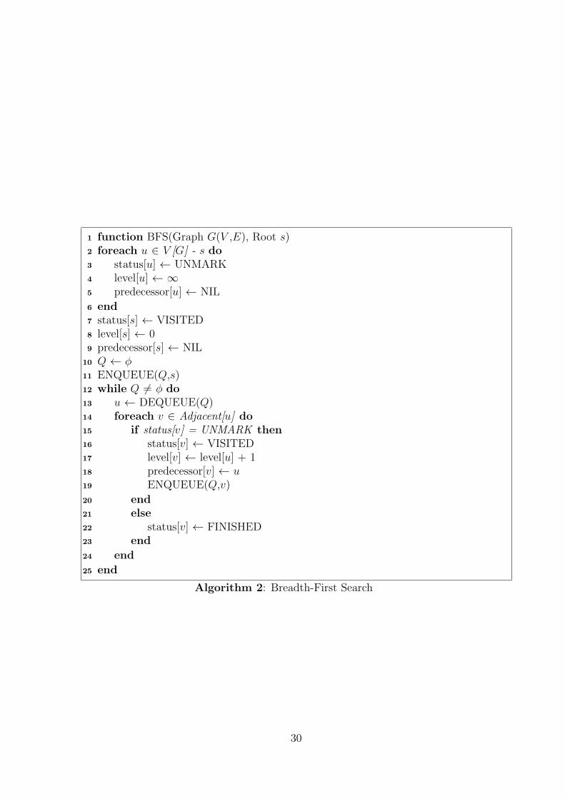
function BFS(Graph G(V ,E), Root s)1

foreach u ∈ V [G] - s do2

status[u] ← UNMARK3

level[u] ← ∞4

predecessor[u] ← NIL5

end6

status[s] ← VISITED7

level[s] ← 08

predecessor[s] ← NIL9

Q ← φ10

ENQUEUE(Q,s)11

while Q 6= φ do12

u ← DEQUEUE(Q)13

foreach v ∈ Adjacent[u] do14

if status[v] = UNMARK then15

status[v] ← VISITED16

level[v] ← level[u] + 117

predecessor[v] ← u18

ENQUEUE(Q,v)19

end20

else21

status[v] ← FINISHED22

end23

end24

end25

Algorithm 2: Breadth-First Search

30

2.3 Problem Formulation

A computation structure is a DAG, G = (V , E), where V is a set of nodes and E is a

set of edges. Each node represents an operation. Edges represent flow of information in

graph as the computation done by one node may be required by another node or set of

nodes. Depending upon whether the producer and consumer are same node or different

nodes, output of a computation needs to be forwarded. As we discussed earlier that it

may be the case that not all nodes of a computation structure, can be executed on a

PE. This problem arises because of inherent configuration of PE. So we need to divide a

computation structure into multiple groups such that each group is capable of executing

on one corresponding PE. Primarily a DAG has a uniform weight distribution for each

edge. Thus we consider weight of each edge as unity. While partitioning we assume that

each edge is of equal weight.

2.3.1 Problem Analysis and Cost Function

A DAG partitioning involves the distribution of operations in such a manner that, execu-

tion of an operation and dependency among operation i.e. computation versus communi-

cation, is balanced. This leads to efficient utilization of resources as well as an improved

program execution. For this, two important factors in consideration are:

i) Temporal dependency i.e how sooner it can be scheduled in time, independent of other

partition sets and,

ii) Communication dependency i.e how many communications one partition set has with

other partition sets.

Through clustering nodes with there parent [1], one can partition graph into groups

of nodes such that they are “more” communication independent but lagging temporal

independence, whereas through an as-soon-as-possible (ASAP) levelling [1] of nodes, one

can partition the graph into groups of nodes such that they exploited the temporal inde-

pendence but lag in communication independence.

31

While designing a cost function, it’s straight forward to account for communication

dependency as it is weight of a cut-set. But incorporating temporal dependency in cost

function is not trivial, as it is measured by execution independence of PEs (or partitioned

groups) in a computation structure and can be determined precisely only at run time.

We use an abstract model of computing system for CGRA as discussed in section 5.1 and

compare the performance with some of the existing approaches.

2.4 Partitioning: A retrospective view

Here we look in the existing approaches for graph partitioning. We explore ways, in which

we can apply these techniques and approaches for DFG partitioning. We can broadly

classify the graph partitioning algorithm in three different categories. First, a simple

and straight forward way of partitioning is checking for all the possible combination of

partitions i.e. exhaustive or combinatorial approach. Second, could be move based one

where we start taking decision at one step and we carry forward it in next step . A third

approach could be a specialized one which is applicable for a special type of problems as

well very much prone to initial conditions for partitions. We take a closer look to all the

three different approaches and will deduce a way which suits our need in best way.

2.4.1 Random or exhaustive or all combinatorial search

One simple and straight forward method for graph partition is to enumerate all possible

combinations of partition sets and then choose one, which has the best value for cost

function. While this method is good for partitioning of smaller graphs, as the graph

size increases, the combinatorial computational complexity increase asymptotically. This

happens because for smaller graphs, total number of enumerations is small but with little

increase in size, number of enumerations increases enormously which lead to over all

computational complexity. In summary exhaustive algorithms are simplest to implement

and work good for relatively “smaller’ graphs. In principle exhaustive search is good for

off-line computation and not preferable for real time usage.

32

2.4.2 Move based Heuristics

Move based heuristic’s works on the principle of local optimum such that, they try locally

to find the best possible solution. All move base heuristics select a designated root as a

starting reference node for the algorithm. This root is added in the first partition set.

Now with respect this root, a neighbour which gives the optimal cost for the cost function

is taken in consideration and added to the set. Iteratively, in each step we add one new

node to the set while considering the optimality of cost function as the base factor. We

do this till, not all the nodes get exhausted and are added to one of the partition set. The

key principle of move based heuristics are that they work on current maxima or optimal.

Examples are Kernighan-Lin [20].

2.4.3 Meta-Heuristics

Meta heuristics are specialized heuristics with a specification that suitably fits in the scope

of algorithm. Simulated Annealing (SA) and Genetic Algorithm (GA) are two examples

in this category.

2.5 Partitioning: Algorithms, Orthogonal Approaches

and Discussion

We discuss two algorithms: Kernighan-Lin and Greedy Graph Growing Partitioning

2.5.1 Kernighan-Lin (KL) Algorithm

The KL [20] algorithm works by iteration. The original KL algorithm attempts to find

bisection of graph G=(V,E) as two disjoint subsets X and Y such that sum T of the

weights of the edges between nodes in X and Y is minimized. For each node an internal

cost INode and an external cost ENode is calculated. Internal cost is sum of the costs of

edges between that node and other nodes in same set. External cost is the sum of costs

of edges between node and nodes in other set. The difference DNode between internal cost

33

and external cost is calculated as,

DNodes = ENode - INode

In each iteration it searches for vertices from each part of the graph such that swapping

them leads to a partition with smaller cost Tmin. If such vertices exists then the swap is

performed and this becomes the partition for next iteration. If x and y are interchanged,

then the reduction in cost is,

Told - Tnew = Dx + Dy - 2cx,y,

Where cx,y is the cost of possible edge between x and y.

KL algorithm continues by repeating the entire process of exchange of elements between

X and Y that maximizes the Told - Tnew. If it cannot find such vertices, algorithm

terminates. KL gives the local minimum and no further improvements can be made by

algorithm itself.

Time complexity for KL algorithm is O(n2logn). KL has been later extended to

k-way partitioning. Advantage of the KL algorithm, is that it has an easy, straight

forward formulation and simple data structures. A disadvantage of KL algorithm is

that it highly depends on the initial partitioning. A bad initial partition for the KL

algorithm will result to a local optimum which might be arbitrarily bad solution. Few later

work [21] incorporate some sort of clustering (compaction or contraction) or similar tactics

in order to avoid getting trapped in a local optimum. The Fiduccia-Mattheyses (FM) [22]

algorithm is one such improvement of KL algorithm. FM worst case computation time per

pass, grows linearly with the size of the graph O(cn), where n is the number of nodes and

c the highest connectivity of the node. This is achieved, as FM algorithm uses efficient

data structures to avoid re-computation of the gain for all nodes like KL.

2.5.2 Greedy Graph Growing Partitioning (GGGP)

Greedy Graph Growing Partitioning (GGGP) is proposed by Karypis and Kumar [23].

This works similar to KL as for each vertex v, gain in the edge-cut can be defined by

inserting v into the growing partition. Further the vertices of graph frontier are ordered

in non-decreasing fashion as per their gain. Thus the vertex which gives the largest

34

decrease in the edge-cut is inserted first. Once a vertex is inserted into partition it’s

neighbors that are already in the frontier are updated and those not in the frontier are

added to frontier. GGGP requires the same data-structures as those required by the KL

algorithm. Only difference between GGGP and KL is that in former rather computing

gains for all the nodes one calculate the gains only for the nodes that are touched by

the frontier. GGGP do not consider the direction of flow of information as per directed

graph that may hinder the temporal independence of partitions and, is also prone to get

trapped by selection of unfavourable initial node.

2.5.3 Two orthogonal approach to partitioning

Along-with algorithms, we focus our discussion on the two orthogonal approaches as given

by Purna et al. [1]. Primarily these two approaches: Level Based Partitioning and Cluster

based Partitioning, gives insight on the fundamental factors that affect the suitability and

performance of a partitioning algorithm:

Level Based Partitioning (LBP)

It works by first classifying the nodes of input application as per their ASAP levels [1].

ASAP levelling helps in exposing the parallelism hidden to the graph nodes. This is

due to the fact that all nodes at same level can be considered for parallel execution.

Also there may exists some degree of parallelism among the nodes at different levels.

This dependency is checked if there exists an edge between them. Level based algorithm

traverses nodes of the graph, level by level and keep on assigning them in a partition. So

same level nodes go in same partition and if the partition is exhausted then the nodes are

assigned to the next partition. The total complexity of the algorithm is O(|V |+ |E|).

Cluster based Partitioning (CBP)

Cluster based partitioning focuses on reducing communication overhead. One way to do

this is to cluster nodes with common parent. So in this algorithm, tendency is to assign

common parent to same partition thus reducing the number of communication overheads.

35

This is done as long as a partition does not get exhausted. This algorithm ensures better

results in reducing communication overhead when compared with level based partitioning.

The total computational complexity is O(|V |+ |E|).

2.5.4 Discussion

From the above discussion we can see that KL is a simple heuristic that gives local

optimum performance. But original KL has high time complexity as well it may get

stuck into local minimum due to poor choice of initial partition. Work has been done

on both fronts by considering i) only selected nodes for the gains and update and, ii) by

choosing multiple initial nodes. This has positive effect on time complexity and hence

algorithm run-time. On other hand, this inherently imposes complexity in implementation

of algorithm. GGGP is a good algorithm with respect to execution time but there is

scope of improvement of overall program execution by better selection of nodes in graph

frontiers and hence a better balance between computation versus communication is sought.

Level-Based Partitioning (LBP) and Cluster-Based Partitioning (CBP) consider the two

extremes with respect to computation versus communication where as a balance is sought

for better program execution. In next section, we present our partitioning algorithm that

tries to balance between LBP and CBP by making a balance between computation versus

communication. We compare our algorithm with the LBP and CBP on an abstracted

CGRA program execution model (refer section 5.1).

2.6 GoPart : A Cluster-Base Level Partitioning

GoPart (Graph oriented Partitioning) is an orientation based partitioning mechanism.

Here “orientation of graph” is apparent as, levelling of nodes are with respect to a root

(or reference) node of graph. Primary objective of our heuristic is to exploit the max-

imum parallelism while keeping the communication cost minimum. In order to do this,

our approach is to club together the nodes that communicate closely and put them in

one partition while considering the levelling of nodes. So that similar and independent

36

partition groups could execute in parallel, in order to exploit the parallelism. We do this

for each new partition and do this until all the nodes are assigned to some partition.

We frequently use following notations, while partitioning a graph.

Partition-Set: This represents the current partition set. We start with an empty par-

tition set. Any new node under consideration is added to this set, which is limited by

the size k of a PE. Once the current partition set is full, another new partition set is

taken. After partitioning process is complete, we will have as many Partition-Set’s as

total number of nodes in the original computation structure divided by the size limit of

PE. So if a DAG consists of n nodes then the total number of partitions will be ⌈ nk⌉.

Neighbor-Set: While we process the graph for partitioning we make a set of neighbors

with respect to nodes already added in Partition-Set. In Neighbor-Set we add the nodes

which are neighbors to nodes in the Partition-Set. Further, these nodes are sorted based

on number of in-edges and out-edges with respect to the nodes of Partition-Set. This

ordering is done with the help of affinity matrix (AM), which we discussed next in this

section. The purpose of Neighbor-Set is to facilitate the future decision process regarding

inclusion of a node in Partition-Set.

Affinity Matrix: We also need a mechanism for selection of one node from the elements

of Neighbor-Set. For this we introduce the notion affinity of a node. Affinity is “degree of

communication” between a node and Partition-Set. We define in-affinity as the weight of

edges through which their is an incoming edge from Partition-Set to the node under con-

sideration. Similarly we define out-affinity as the weight of edges through which their is

an outgoing edge from node to Partition-Set. Affinity of a node is total sum of in-affinity

and out-affinity. We construct affinity matrix with respect to Partition-set and only for

the elements in Neighbor-Set.

Example: In figure 2.4, let node N1 is selected as root and partition-set has N1,N2

nodes. Nodes N3, N4 and N6 are its neighbors. Affinity matrix for this is shown in

table 2.1.

GoPart is a three step construction. Pre-partition phase of compiler [24] gives the

37

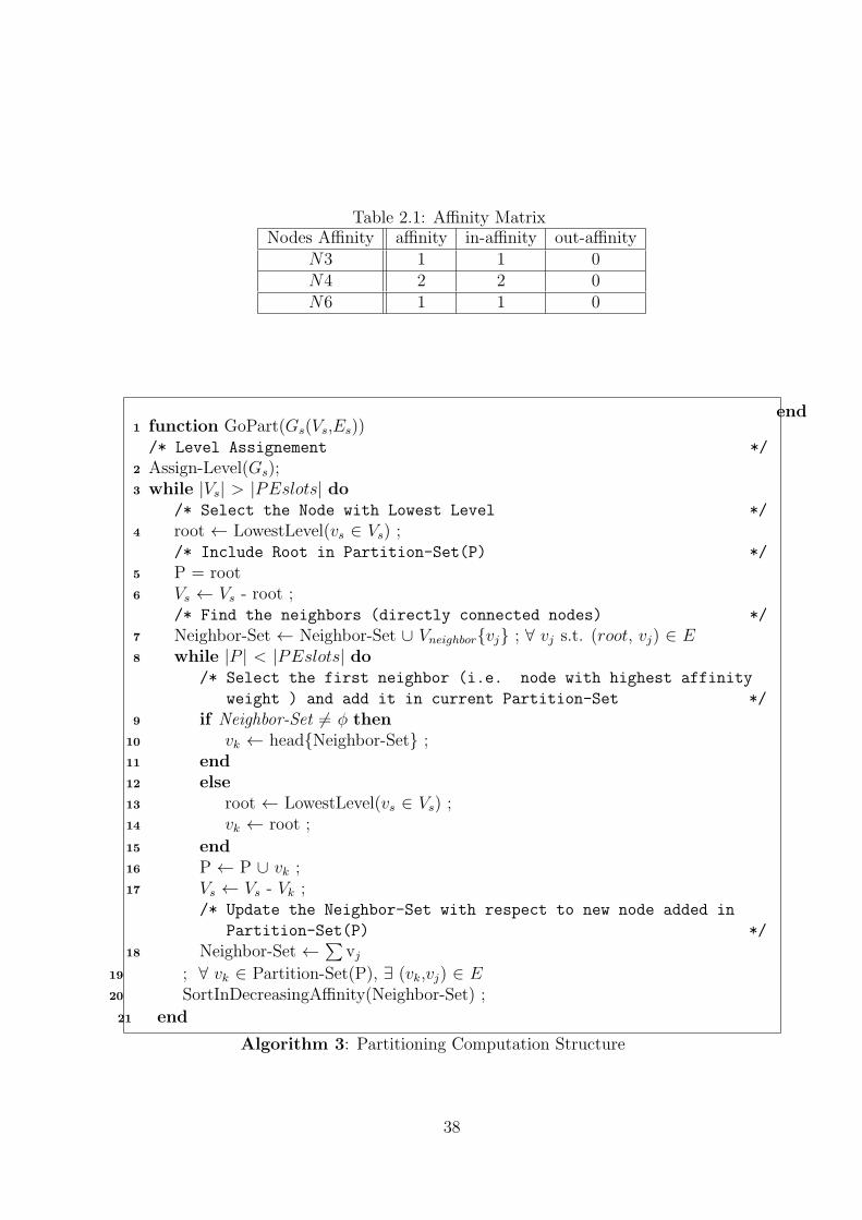
Table 2.1: Affinity MatrixNodes Affinity affinity in-affinity out-affinity

N3 1 1 0N4 2 2 0N6 1 1 0

function GoPart(Gs(Vs,Es))1

/* Level Assignement */

Assign-Level(Gs);2

while |Vs| > |PEslots| do3

/* Select the Node with Lowest Level */

root ← LowestLevel(vs ∈ Vs) ;4

/* Include Root in Partition-Set(P) */

P = root5

Vs ← Vs - root ;6

/* Find the neighbors (directly connected nodes) */

Neighbor-Set ← Neighbor-Set ∪ Vneighbor{vj} ; ∀ vj s.t. (root, vj) ∈ E7

while |P | < |PEslots| do8

/* Select the first neighbor (i.e. node with highest affinity

weight ) and add it in current Partition-Set */

if Neighbor-Set 6= φ then9

vk ← head{Neighbor-Set} ;10

end11

else12

root ← LowestLevel(vs ∈ Vs) ;13

vk ← root ;14

end15

P ← P ∪ vk ;16

Vs ← Vs - Vk ;17

/* Update the Neighbor-Set with respect to new node added in

Partition-Set(P) */

Neighbor-Set ←∑

vj18

; ∀ vk ∈ Partition-Set(P), ∃ (vk,vj) ∈ E19

SortInDecreasingAffinity(Neighbor-Set) ;20

end21

end

Algorithm 3: Partitioning Computation Structure

38

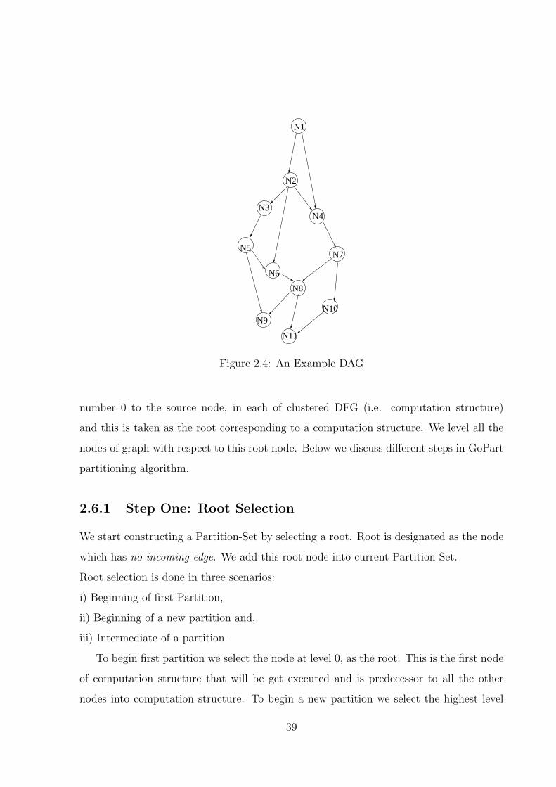
N9

N1

N2

N3N4

N11

N8

N7

N10

N6

N5

Figure 2.4: An Example DAG

number 0 to the source node, in each of clustered DFG (i.e. computation structure)

and this is taken as the root corresponding to a computation structure. We level all the

nodes of graph with respect to this root node. Below we discuss different steps in GoPart

partitioning algorithm.

2.6.1 Step One: Root Selection

We start constructing a Partition-Set by selecting a root. Root is designated as the node

which has no incoming edge. We add this root node into current Partition-Set.

Root selection is done in three scenarios:

i) Beginning of first Partition,

ii) Beginning of a new partition and,

iii) Intermediate of a partition.

To begin first partition we select the node at level 0, as the root. This is the first node

of computation structure that will be get executed and is predecessor to all the other

nodes into computation structure. To begin a new partition we select the highest level

39

(lowest numerical value) node that is not included into a partition. This serves as the

first node in Partition-Set. If the nodes in Partition-Set do not have any neighbors but

there are still nodes to be considered then we select a root. We select node at the highest

level as the root and add it to the Partition-Set.

With respect to root node, we find all the communicating nodes. These nodes are

“neighbor” nodes. We put all neighbors in Neighbor-Set.

2.6.2 Step Two: Updating Neighbor-Set and Affinity matrix

If the Partition-Set is not exhausted then it can accommodate more nodes. If Neighbor-

Set is not empty, we select most affine node from Neighbor-Set. This selection is done

from affinity matrix on the basis of affinity as discussed above. If affinity is same for

more than one node, then we prioritize the nodes based on their higher in-affinity. In case

of equal in-affinity value, we chose the node from lower level ( i.e. higher value level).

The selected node is added to current Partition-Set. If Neighbor-Set is empty, we find a

new root from existing nodes. This designated root we find by selecting the node from

the lowest level. So Based on this, affinity-matrix is updated after a node gets added in

Partition-Set. If the current Partition-Set is exhausted, we begin with a new partition.

So a root is selected as the start of this new partition set and then on we repeat the

procedure, as in section 2.6.1.

2.6.3 Step Three: Iteration

Once a new node is added in Partition-Set, we rebuild the Neighbor-Set with respect to

all the nodes in current Partition-Set. We choose the highest affine node from Neighbor-

Set and add it to Partition-Set. We iteratively repeat this process i.e. root selection (if

needed), updating Neighbor-Set, updating the affinity-matrix, being new Partition-Set,

unless or until current Partition-Set has exhausted it’s limit or all the nodes of DAG are

placed into Partition-Set’s.

Pseudo code for Partition-Set construction is given in algorithm 3.

40

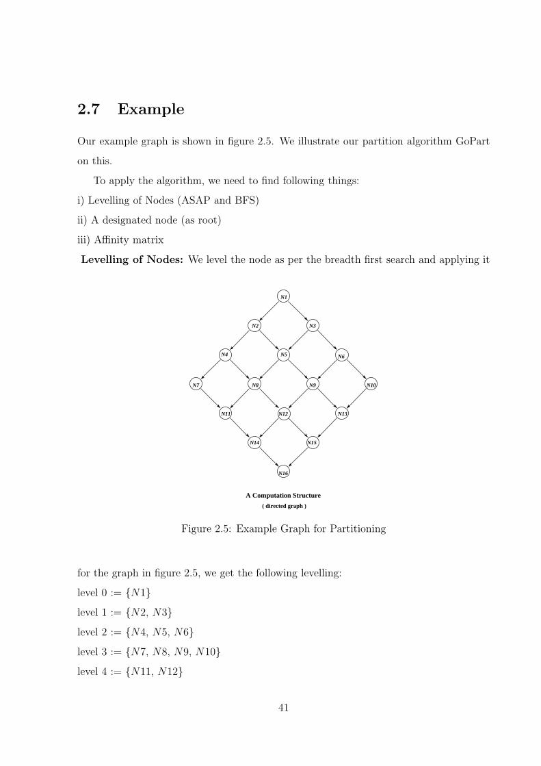
2.7 Example

Our example graph is shown in figure 2.5. We illustrate our partition algorithm GoPart

on this.

To apply the algorithm, we need to find following things:

i) Levelling of Nodes (ASAP and BFS)

ii) A designated node (as root)

iii) Affinity matrix

Levelling of Nodes: We level the node as per the breadth first search and applying it

( directed graph )

N1

N2 N3

N4 N5 N6

N7 N8 N9 N10

N11 N12 N13

N14 N15

N16

A Computation Structure

Figure 2.5: Example Graph for Partitioning

for the graph in figure 2.5, we get the following levelling:

level 0 := {N1}level 1 := {N2, N3}level 2 := {N4, N5, N6}level 3 := {N7, N8, N9, N10}level 4 := {N11, N12}

41

level 5 := {N13, N14, N15}level 6 := {N16}Root Selection: Root node is added in three cases i) At the start of algorithm for first

partition, ii) Start of a new partition and, ii) while adding nodes in a partition set if

neighbor set is empty but not all vertices of Vs have been placed.

CONSTRAINTS:

partition size = 4

INITIALS :

total node = 16

NodesInCurrentPartitionSet = φ

STEP 1:

As total no of nodes (=16) is greater than the partition size (=4), so partitioning is

needed.

Finding the root: We choose the node at level 0 as the root. Root selection in future

iterations will be based on levelling of nodes. Here N1 is the designated root in our case.

NodesInCurrentPartitionSet = {N1}NodesInCurrentPartitionSet = 1

NodesNotInPartition = 15

NeighborSet = {N2, N3}STEP 2:

NodesInCurrentPartitionSet < PartitionSize , we will add more nodes to partition set

from NeighborSet. At each step this condition will be tested.

N2 is considered next for inclusion into NodesInCurrentPartitionSet.

NodesInCurrentPartitionSet = {N1, N2}NodesInCurrentPartitionSet = 2

NodesNotInPartition = 14

NeighborSet = {N3, N4, N5}Note: We also reorder NeighborSet = {N4, N5, N3} as we always choose first element

from NeighborSet and ordering within NeighborSet is based on decreasing affinity weight.

42

Therefore higher affinity weight node comes first.

NeighborSet = {N4, N5, N3}STEP 3:

NodesInCurrentPartitionSet < PartitionSize(4) , we will add more node in partition set

from NeighborSet.

N4 is considered next for inclusion into NodesInCurrentPartitionSet.

NodesInCurrentPartitionSet = {N1, N2, N4}NodesInCurrentPartitionSet = 3

NodesNotInPartition = 13

NeighborSet = {N3, N5, N7, N8}After reorder NeighborSet = {N7, N8, N3, N5}STEP 4:

NodesInCurrentPartitionSet < PartitionSize(4) , we will add more node in partition set

from NeighborSet.

N7 is considered next for inclusion into NodesInCurrentPartitionSet.

NodesInCurrentPartitionSet = {N1, N2, N4, N7}NodesInCurrentPartitionSet = 4

NodesNotInPartition = 12

NeighborSet = {N3, N5, N8, N11}STEP 5:

Condition NodesInCurrentPartitionSet(4) < PartitionSize(4) fails.

So we check if NodesNotInPartition > PartitionSize, which TRUE. So a new PartitionSet

= φ and NeighborSet = φ is taken.

Root Selection: N3 is selected based on criteria defined above.

NodesInCurrentPartitionSet = {N3}NodesInCurrentPartitionSet = 1

NodesNotInPartition = 11

NeighborSet = {N5, N6}STEP 6:

43

NodesInCurrentPartitionSet < PartitionSize(4) , we will add more node in partition set

from NeighborSet.

N5 is considered next for inclusion into NodesInCurrentPartitionSet.

NodesInCurrentPartitionSet = {N3, N5}NodesInCurrentPartitionSet = 2

NodesNotInPartition = 10

NeighborSet = {N6, N8, N9}STEP 7:

NodesInCurrentPartitionSet < PartitionSize(4) , we will add more node in partition set

from NeighborSet.

N8 is considered next for inclusion into NodesInCurrentPartitionSet.

NodesInCurrentPartitionSet = {N3, N5, N8}NodesInCurrentPartitionSet = 3

NodesNotInPartition = 9

NeighborSet = {N6, N9, N11, N12}STEP 8:

NodesInCurrentPartitionSet < PartitionSize(4), we will add more node in partition set

from NeighborSet.

N11 is considered next for inclusion into NodesInCurrentPartitionSet.

NodesInCurrentPartitionSet = {N3, N5, N8, N11}NodesInCurrentPartitionSet = 4

NodesNotInPartition = 8

NeighborSet = {N6, N9, N12, N14}STEP 9:

Condition NodesInCurrentPartitionSet(4) < PartitionSize(4) fails.

So we check if NodesNotInPartition > PartitionSize, which TRUE. So a new PartitionSet

= φ and NeighborSet = φ is taken.

Root Selection: N6 is selected based on criteria defined above.

NodesInCurrentPartitionSet = {N6}

44

NodesInCurrentPartitionSet = 1

NodesNotInPartition = 7

NeighborSet = {N9, N10}STEP 10:

NodesInCurrentPartitionSet < PartitionSize(4) , we will add more node in partition set

from NeighborSet.

N9 is considered next for inclusion into NodesInCurrentPartitionSet.

NodesInCurrentPartitionSet = {N6, N9}NodesInCurrentPartitionSet = 2

NodesNotInPartition = 6

NeighborSet = {N10, N12, N13}STEP 11:

NodesInCurrentPartitionSet < PartitionSize(4) , we will add more node in partition set

from NeighborSet.

N10 is considered next for inclusion into NodesInCurrentPartitionSet.

NodesInCurrentPartitionSet = {N6, N9, N10}NodesInCurrentPartitionSet = 3

NodesNotInPartition = 5

NeighborSet = {N12, N13}STEP 12:

NodesInCurrentPartitionSet < PartitionSize(4), we will add more node in partition set

from NeighborSet.

N13 is considered next for inclusion into NodesInCurrentPartitionSet.

NodesInCurrentPartitionSet = {N6, N9, N10, N13}NodesInCurrentPartitionSet = 4

NodesNotInPartition = 4

NeighborSet = {N12, N15}STEP 13:

So we check if NodesNotInPartition > PartitionSize, which also fail. So a new PartitionSet

45

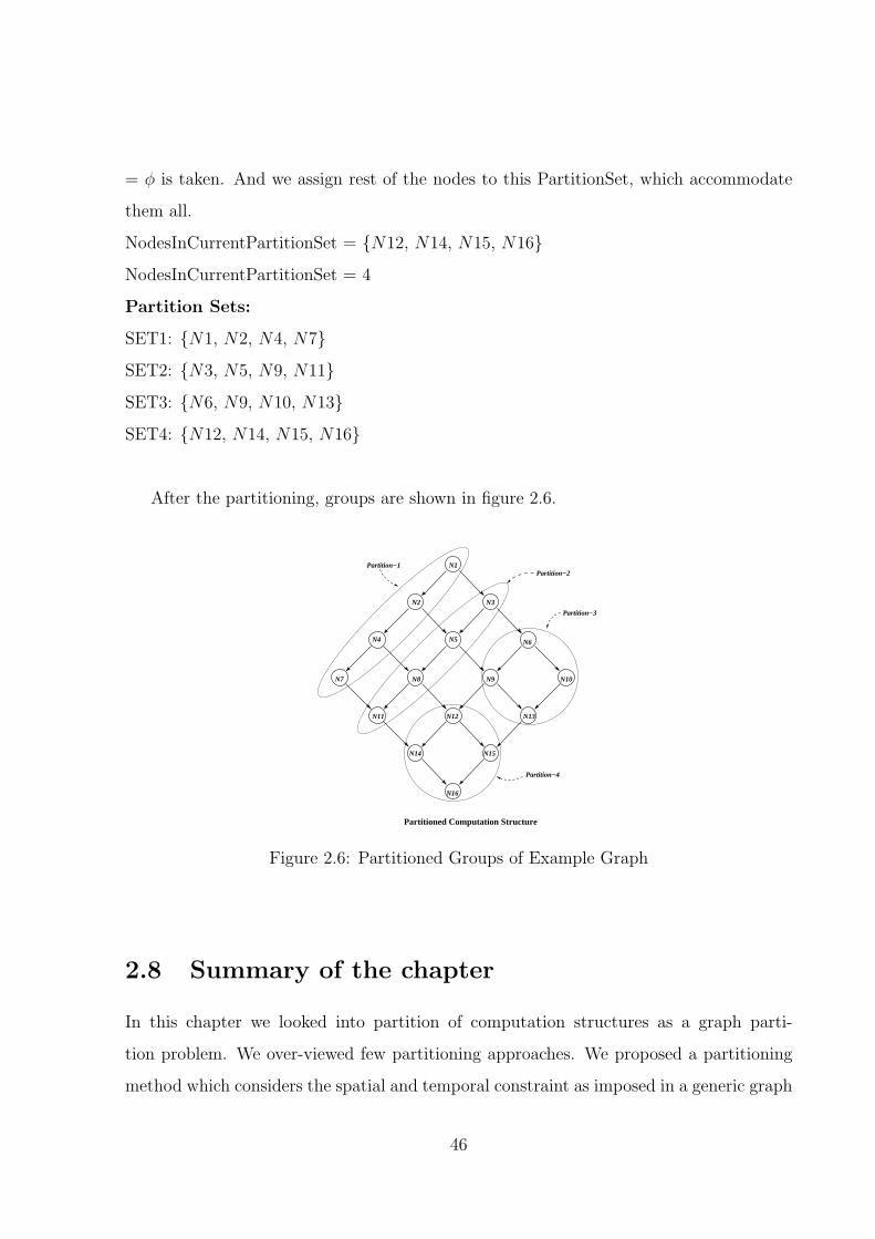
= φ is taken. And we assign rest of the nodes to this PartitionSet, which accommodate

them all.

NodesInCurrentPartitionSet = {N12, N14, N15, N16}NodesInCurrentPartitionSet = 4

Partition Sets:

SET1: {N1, N2, N4, N7}SET2: {N3, N5, N9, N11}SET3: {N6, N9, N10, N13}SET4: {N12, N14, N15, N16}

After the partitioning, groups are shown in figure 2.6.

Partition−3

N1

N2 N3

N4 N5 N6

N7 N8 N9 N10

N11 N12 N13

N14 N15

N16

Partitioned Computation Structure

Partition−1Partition−2

Partition−4

Figure 2.6: Partitioned Groups of Example Graph

2.8 Summary of the chapter

In this chapter we looked into partition of computation structures as a graph parti-

tion problem. We over-viewed few partitioning approaches. We proposed a partitioning

method which considers the spatial and temporal constraint as imposed in a generic graph

46

partitioning. This partitioned computation structure gets executed on a CGRA. After

partitioning we have an interconnection of set of partitioned blocks. This is referred to

as communication graph. In next chapter we discuss mapping of this communication (or

interconnection) graph onto target topology.

47

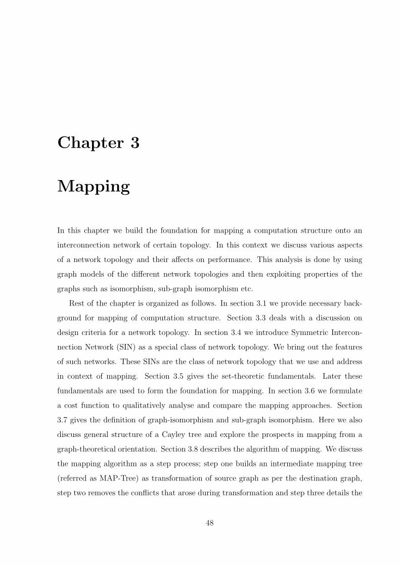
Chapter 3

Mapping

In this chapter we build the foundation for mapping a computation structure onto an

interconnection network of certain topology. In this context we discuss various aspects

of a network topology and their affects on performance. This analysis is done by using

graph models of the different network topologies and then exploiting properties of the

graphs such as isomorphism, sub-graph isomorphism etc.

Rest of the chapter is organized as follows. In section 3.1 we provide necessary back-

ground for mapping of computation structure. Section 3.3 deals with a discussion on

design criteria for a network topology. In section 3.4 we introduce Symmetric Intercon-

nection Network (SIN) as a special class of network topology. We bring out the features

of such networks. These SINs are the class of network topology that we use and address

in context of mapping. Section 3.5 gives the set-theoretic fundamentals. Later these

fundamentals are used to form the foundation for mapping. In section 3.6 we formulate

a cost function to qualitatively analyse and compare the mapping approaches. Section

3.7 gives the definition of graph-isomorphism and sub-graph isomorphism. Here we also

discuss general structure of a Cayley tree and explore the prospects in mapping from a

graph-theoretical orientation. Section 3.8 describes the algorithm of mapping. We discuss

the mapping algorithm as a step process; step one builds an intermediate mapping tree

(referred as MAP-Tree) as transformation of source graph as per the destination graph,

step two removes the conflicts that arose during transformation and step three details the

48

resource matrix generation.

3.1 Background

In the previous chapter we formulated a technique for partitioning of computation struc-

tures. A partitioned computation structure is an interconnection of nodes. A node is

referred to as a compute-block and a link in interconnection represents communication

between two compute-blocks. Weight of the link represents the number of communica-

tion between two compute-blocks. We refer to this interconnection of compute-blocks as

a communication graph (CG).

In CGRA, a computation structure is executed by a group of PEs. These PEs are

connected in a particular fashion that forms the topology of interconnection network. Flow

of information among PEs is achieved through interconnection network. Thus network-

topology plays an important role in the course of execution. Granularity of execution is

such that a compute-block is executed on one PE. Thus a PE can be considered as a

resource and hence we refer to the interconnection network of PEs as RG. In order to

(iii) Mapping

a

b

c

A

CB

A

B C

(i) Computation Structure (ii) Resource Graph

Figure 3.1: Mapping of a Computation Structure on a Network Topology

execute the instructions in a compute-block, a compute-block needs to be placed on a

PE. As compute-blocks are outcomes of partitioning of computation structures we need

to map computation structures onto a network-topology. The complete process translates

into imposition of a CG onto an RG. There may be structural differences between the

CG and RG. This hinders the direct imposition of CG onto RG. Thus necessitating the

transformation of CG to an intermediate graph, in order to fulfil the structural constraint

of RG. Figure 3.1 shows mapping of a triangular communication graph onto a mesh

49

network.

3.2 Related Work

One variant of Graph Mapping is approached as a graph embedding problem. In such cases

drawing of a graph on a surface takes place in such a fashion that edge are intersecting

only at the end points. Another variant comes through fixing the topology of source and

target graphs which further adds the dimension to design of a mapping algorithm. As

Garey and Johnson [15] discussed graph mapping as an NP problem in its generality,

various approaches (as we see below) and variant to this problem has been followed to

achieve sub-optimal performance.

3.2.1 Dimension reductionist approach

In application space of web graphs, graph embedding is achieved through standard dimen-

sion reduction problem where techniques such as Reimannian [25], Isomaps [26], Locally

linear embedding [27], locality preserving projection [28] has been used.

3.2.2 Fix topologies of source and target graph

In certain applications such as processor-processor allocation, the structure of source graph

as well target graph is fix. In such cases one can exploit the properties of the topology

to the advantageous of the mapping. For example, hypercube is commonly mapped on a

2-D mesh [29]. The other combinations that also suits such study are: hypercube on 3-D

Mesh [29], Meshes of Trees into de-Bruijn Graphs [30], linear array to hypercube etc.

3.2.3 Mapping as a Generic Framework

Koziris [31] and Zhonghai [32] has discussed the mapping in its generality, to come up

with a mapping algorithm that fits to all class of problems. They defined cost function

as the summation over the product of communication weight and distance between the

50

groups- which is essentially the routing cost. Objective function in such cases has been the

minimization of total routing cost. Though, previous works such as Koziris [31], Zhonghai

[32] has not exploited the uniform degree property of target graphs that gets instantiated

with each target graph, we intend to explore the mapping with this perspective.

We will see in section 3.7 that focus of our work is on developing a framework that

suits a generic class of mapping. Reasons we took this approach are:

1) Source graph is random in nature so nothing can be say about its topology.

2) Focus of our study are CGRAs. A CGRA uses symmetric interconnection network as

target topology. So we took different degree symmetric interconnection networks as our

target graphs and that gives the generalization to the mapping.

Thus thematic representation of our mapping work is, to come up with a framework

that maps a random source graph to a fix degree target graph where the degree of target

graph itself can be varied.

3.3 Interconnection Network Design Parameters

An interconnection network provides the physical structure for flow of information among

the PEs. This flow is affected by various factors like; number of communication links

between source and destination, distance between source and destination, congestion in

the network, diameter of network, routing algorithm etc. A network topology is designed

with certain objectives and features. In this section we briefly discuss few of design

parameters that one should consider before choosing a network topology for PEs.

3.3.1 Number of Edges in Network

Number of edges directly translates into number of wires on NoC. More wires led to faster

communication between nodes. For example in a complete graph topology each node is

connected to every other node. This guarantees one-step communication between any two

nodes. In a linear array topology, nodes are connected in serial fashion. So communication

between two nodes require as many steps as the number of nodes between them.

51

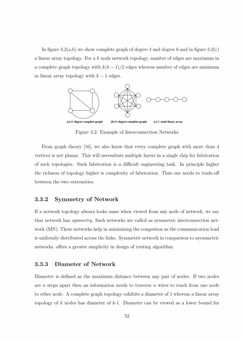
In figure 3.2(a,b) we show complete graph of degree 4 and degree 6 and in figure 3.2(c)

a linear array topology. For a k node network topology, number of edges are maximum in

a complete graph topology with k(k− 1)/2 edges whereas number of edges are minimum

in linear array topology with k − 1 edges.

(c) 5−node linear array(b) 6−degree complete graph(a) 4−degree complete graph

Figure 3.2: Example of Interconnection Networks

From graph theory [16], we also know that every complete graph with more than 4

vertices is not planar. This will necessitate multiple layers in a single chip for fabrication

of such topologies. Such fabrication is a difficult engineering task. In principle higher

the richness of topology higher is complexity of fabrication. Thus one needs to trade-off

between the two extremities.

3.3.2 Symmetry of Network

If a network topology always looks same when viewed from any node of network, we say

that network has symmetry. Such networks are called as symmetric interconnection net-

work (SIN). These networks help in minimizing the congestion as the communication load

is uniformly distributed across the links. Symmetric network in comparison to asymmetric

networks, offers a greater simplicity in design of routing algorithm.

3.3.3 Diameter of Network

Diameter is defined as the maximum distance between any pair of nodes. If two nodes

are n steps apart then an information needs to traverse n wires to reach from one node

to other node. A complete graph topology exhibits a diameter of 1 whereas a linear array

topology of k nodes has diameter of k-1. Diameter can be viewed as a lower bound for

52

worst-case latency of a routing algorithm. Thus reduction in diameter from k to 1 also

lessens worst-case communication delay by a factor of k. This implies that networks with

small diameters are preferable.

3.3.4 Degree of Node

The number of nodes to which a node is connected defines the degree of that node. Based

on degree of nodes, a network could be homogeneous or heterogeneous. If all the nodes

have same degree then a network is homogeneous otherwise network is heterogeneous. A

node has maximum degree when it is connected to all other nodes of network. In case of

network of n nodes, this value is n-1. A complete graph is topology where all the nodes

have the maximum degree. Nodes in linear array have degree of 1 and 2 (refer figure

3.2(c)).

3.3.5 Bisection Width

This is defined as the minimum number of wires that needs to be remove for bisecting

a network. Consider we have two threads executing on different parts of the RG. As

each thread is getting executed by a group of PEs (nodes), the dependent information

is required to transfer from one thread to another thread. In such case, bisection width

gives the maximum number of channels of communication (edges) available for this. Thus

larger the bisection width, more is the number of channels for data transfer.

3.3.6 I/O bandwidth

I/O bandwidth refers to the number of input/output lines to/from the network. These

lines insert data into the network and take result out of the network. This is of particular

importance for solving problems where transport latency of instruction and data domi-

nates over actual execution latency. These lines are added at the periphery of network.

Discussion, Conflicts and Conclusion: Based on above aspects of a network, we

53

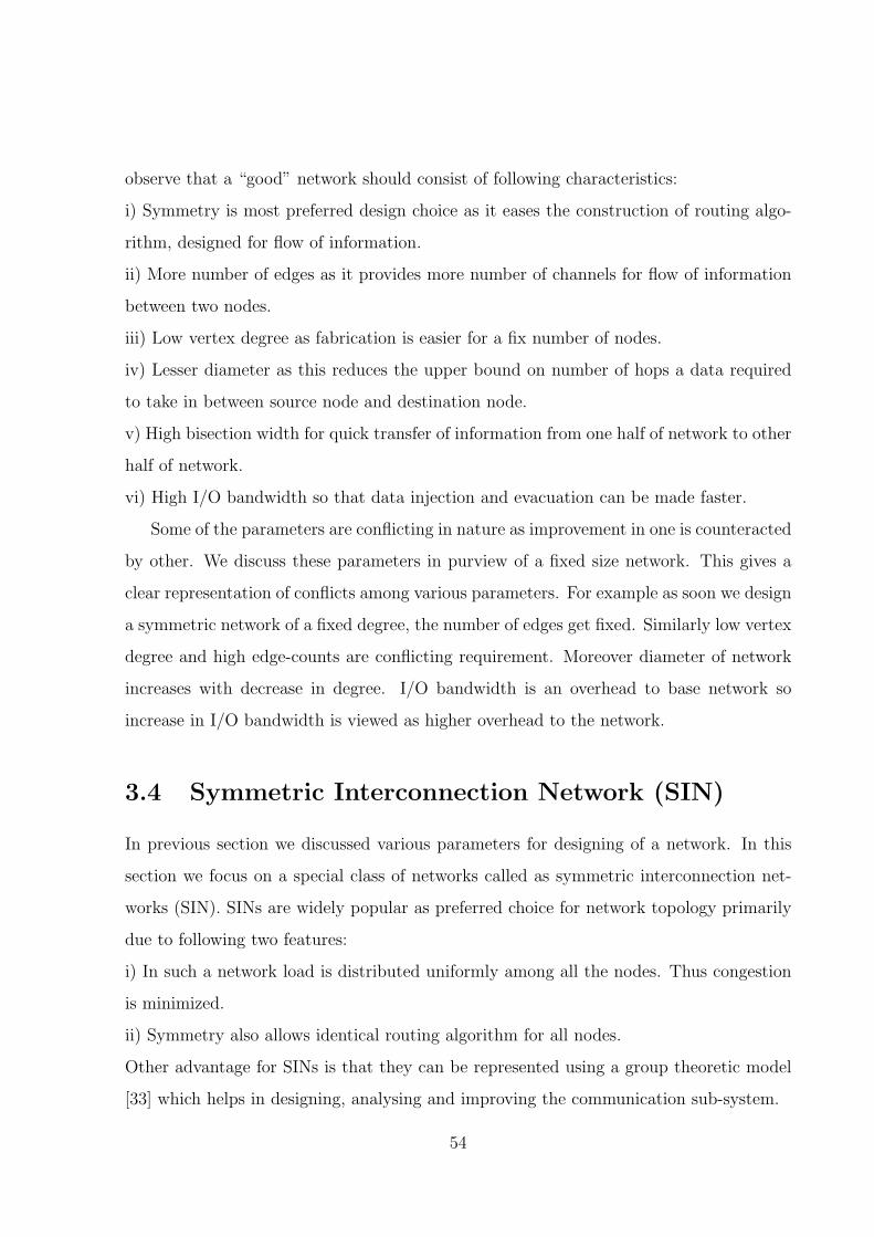
observe that a “good” network should consist of following characteristics:

i) Symmetry is most preferred design choice as it eases the construction of routing algo-

rithm, designed for flow of information.

ii) More number of edges as it provides more number of channels for flow of information

between two nodes.

iii) Low vertex degree as fabrication is easier for a fix number of nodes.

iv) Lesser diameter as this reduces the upper bound on number of hops a data required

to take in between source node and destination node.

v) High bisection width for quick transfer of information from one half of network to other

half of network.

vi) High I/O bandwidth so that data injection and evacuation can be made faster.

Some of the parameters are conflicting in nature as improvement in one is counteracted

by other. We discuss these parameters in purview of a fixed size network. This gives a

clear representation of conflicts among various parameters. For example as soon we design

a symmetric network of a fixed degree, the number of edges get fixed. Similarly low vertex

degree and high edge-counts are conflicting requirement. Moreover diameter of network

increases with decrease in degree. I/O bandwidth is an overhead to base network so

increase in I/O bandwidth is viewed as higher overhead to the network.

3.4 Symmetric Interconnection Network (SIN)

In previous section we discussed various parameters for designing of a network. In this

section we focus on a special class of networks called as symmetric interconnection net-

works (SIN). SINs are widely popular as preferred choice for network topology primarily

due to following two features:

i) In such a network load is distributed uniformly among all the nodes. Thus congestion

is minimized.

ii) Symmetry also allows identical routing algorithm for all nodes.

Other advantage for SINs is that they can be represented using a group theoretic model

[33] which helps in designing, analysing and improving the communication sub-system.

54

A Honeycomb

01

2

3

4

5

670

1

2 3

54

6

7 8

9

10

11

12

13

14 15 16

17

1918

20 21 22

23 24

3−degree Hypercube

Figure 3.3: Examples of Symmetric Interconnection Network (SIN)

The overall construction for SINs have been small degree and diameter, and high

connectivity, bisection width and I/O bandwidth. Example of network topologies, used

for SINs are mesh [18], honeycomb [19], hypercube [18] etc. Graph for hypercube and

honeycomb is shown in figure 3.3. In next chapter we revisit honeycomb and mesh as

example SIN to elaborate our mapping algorithm.

3.5 Mapping: A Set-Theoretic Foundation

In this section we briefly discuss the notion of function that will be used to build the

foundation for solving the mapping problem.

3.5.1 Function

Functions are rules that bring correspondence between two sets. The set of elements

that seeks the correspondence is called domain and the set of elements onto which the

correspondence achieved is called co-domain. From each element of domain X there is

correspondingly one and only one element in co-domain Y . An element in co-domain

that corresponded by an element in domain, is called an image. So images are output

expression from co-domains.

55

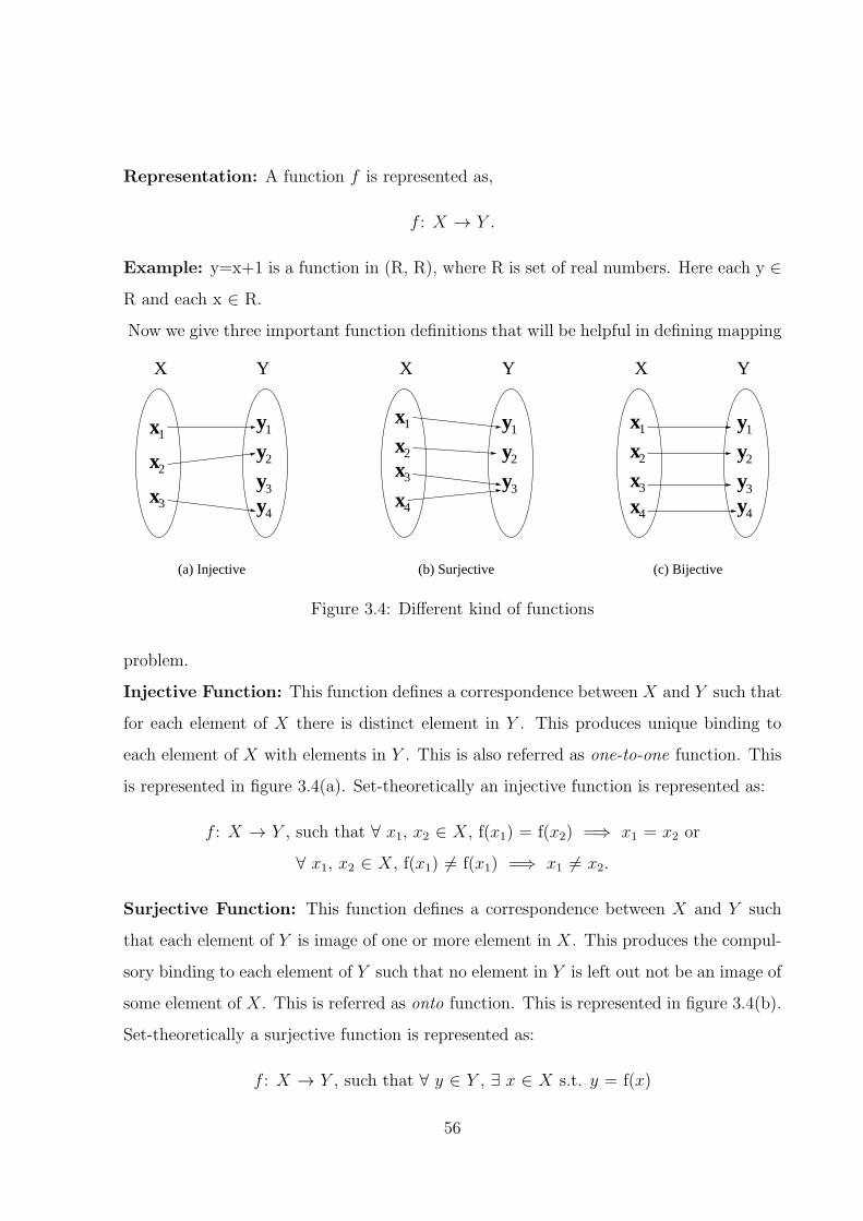
Representation: A function f is represented as,

f : X → Y .

Example: y=x+1 is a function in (R, R), where R is set of real numbers. Here each y ∈R and each x ∈ R.

Now we give three important function definitions that will be helpful in defining mapping

x

(a) Injective (c) Bijective(b) Surjective

x1

x2

x3

yy2

y3

y4

1

X Y

yy2

y3

1

X Y

yy2

y3

y4

1

X Y

x1

x2

3x

x4

x1

x2

x3

4

Figure 3.4: Different kind of functions

problem.

Injective Function: This function defines a correspondence between X and Y such that

for each element of X there is distinct element in Y . This produces unique binding to

each element of X with elements in Y . This is also referred as one-to-one function. This

is represented in figure 3.4(a). Set-theoretically an injective function is represented as:

f : X → Y , such that ∀ x1, x2 ∈ X, f(x1) = f(x2) =⇒ x1 = x2 or

∀ x1, x2 ∈ X, f(x1) 6= f(x1) =⇒ x1 6= x2.

Surjective Function: This function defines a correspondence between X and Y such

that each element of Y is image of one or more element in X. This produces the compul-

sory binding to each element of Y such that no element in Y is left out not be an image of

some element of X. This is referred as onto function. This is represented in figure 3.4(b).

Set-theoretically a surjective function is represented as:

f : X → Y , such that ∀ y ∈ Y , ∃ x ∈ X s.t. y = f(x)

56

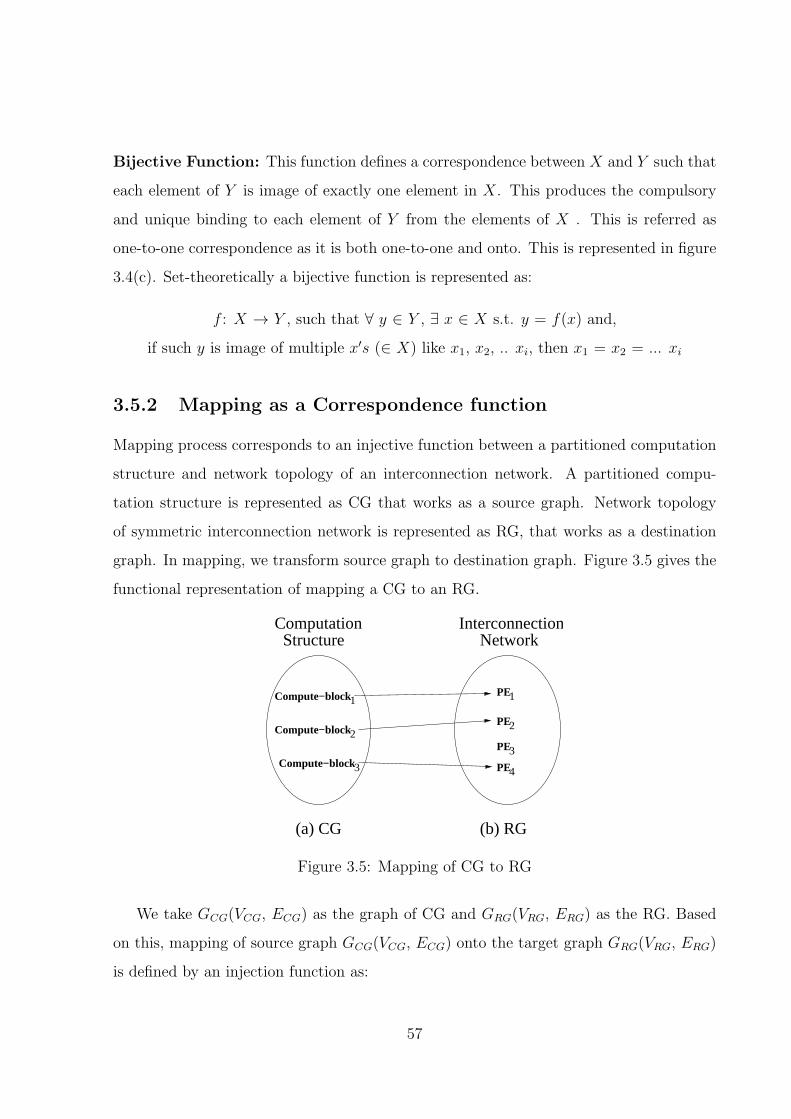
Bijective Function: This function defines a correspondence between X and Y such that

each element of Y is image of exactly one element in X. This produces the compulsory

and unique binding to each element of Y from the elements of X . This is referred as

one-to-one correspondence as it is both one-to-one and onto. This is represented in figure

3.4(c). Set-theoretically a bijective function is represented as:

f : X → Y , such that ∀ y ∈ Y , ∃ x ∈ X s.t. y = f(x) and,

if such y is image of multiple x′s (∈ X) like x1, x2, .. xi, then x1 = x2 = ... xi

3.5.2 Mapping as a Correspondence function

Mapping process corresponds to an injective function between a partitioned computation

structure and network topology of an interconnection network. A partitioned compu-

tation structure is represented as CG that works as a source graph. Network topology

of symmetric interconnection network is represented as RG, that works as a destination

graph. In mapping, we transform source graph to destination graph. Figure 3.5 gives the

functional representation of mapping a CG to an RG.

(b) RG

Structure Network

Compute−block

PE1

PE

PE

PE

2

3

4

2

Compute−block3

Compute−block1

Computation Interconnection

(a) CG

Figure 3.5: Mapping of CG to RG

We take GCG(VCG, ECG) as the graph of CG and GRG(VRG, ERG) as the RG. Based

on this, mapping of source graph GCG(VCG, ECG) onto the target graph GRG(VRG, ERG)

is defined by an injection function as:

57

fmap: VCG 7→ VRG,

such that, ∀ vCGi∈ VCG, ∃! vRGj

∈ VRG,

where, | VCG |≤| VRG |

Each vertex vCG (∈ VCG) is a compute-block and each vertex vRG (∈ VRG) is a PE

and we embed one compute-block onto one PE.

3.6 Cost Function

To evaluate our technique, we define a cost function (CostFunction), similar to the kind

of cost function used in Koziris [31] and Zhonghai [32]. Cost function is defined in such

a manner that it intuitively compare the performance with optimal case. This objective

translates to keeping the communication edges intact as close as they are in source graph.

CostFunction(fmap) =Σ dist(fmap(uCGi), fmap(uCGj

))× commWt(uCGi, uCGj

)

where:

• dist(fmap(uCGi), fmap(uCGj

)) gives the shortest distance between the two nodes (uRGm, uRGn

)

in target graph onto which nodes (uCGi, uRGj

) in the source graph are mapped. Distance

between two adjacent nodes in RG is taken as unit.

• commWt(uCGi, uCGj

) is the weight of the edge euCGi,uCGj

in the source graph. Weight

of an edge in CG, represents the total number of message exchanges between the end

nodes i.e. total number of communication between two compute-block.

Case of Optimal: When all the compute-block of CG gets placed on PEs in exactly the

same fashion as they are in CG, then that is the optimal solution for CG. Function of

optimality i.e. fOptimalmap is defined as :

CostFunction(fOptimalmap ) = min { CostFunction(fmap) ∀ fmap ∈ MAPALL }

where MAPALL is the set of all possible mapping exist for this particular target graph.

•Cost Overhead: Our objective is to find mapping fmap which minimizes CostFunction(fmap).

We compute cost overhead as percentage ratio of, cost difference of mapping algorithm

58

with the optimal, to that of the cost of optimal.

Cost Overhead =(

CostFunction(fmap)−CostFunction(fOptimalmap )

CostFunction(fOptimalmap )

× 100)

%

3.7 Graph Modelling: Salient features and prospects

in Mapping

This section starts with graph description of CG. We also give the data-structure to

represent this. We also describe isomorphic graphs and homomorphic graphs so that

we can bring out isomorphism or subgraph isomorphism of some special kind of graphs

(Cayley tree in our case) with the SINs. We discuss Cayley tree and their generic structure.

Further we bring out the similarity between the SINs and a Cayley tree. This resemblance

is used for exploration of graph mapping in context of SINs.

3.7.1 Communication Graph (CG)

A communication graph (CG) is source graph in mapping. This source graph needs to

be mapped onto SIN. Thus SIN acts as a destination graph. CG is a weighted undirected

graph. An edge represents the communication between two compute-blocks. Weight

represents the number of communication between two compute-blocks. An example CG

is represented in figure 4.7.

3.7.2 Isomorphic Graphs

Isomorphism is an attribute of graphs in which there exists an equivalence between two

graphs. Two graphs G(V,E) and G′(V ′, E ′) are said to be isomorphic and expressed as

G G’ , if there exists a bijection i.e. one-to-one correspondence function, such that,

f : V → V ′, where ∀ u, v ∈ V , {u, v} ∈ E ⇔ ∃ f(u), f(v) ∈ V ′ and {f(u), f(v)} ∈ E ′

This is interpreted as, there is an edge between two vertices in one graph, if and only

if there is a corresponding edge between the corresponding vertices in the other graph.

59

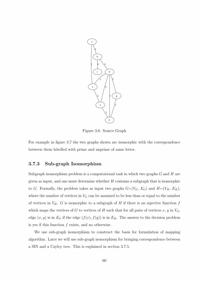
a

b

2

e

1

c

4

d

3

2

f

4

g

3

h

15

2

2

Figure 3.6: Source Graph

For example in figure 3.7 the two graphs shown are isomorphic with the correspondence

between them labelled with prime and unprime of same letter.

3.7.3 Sub-graph Isomorphism

Subgraph isomorphism problem is a computational task in which two graphs G and H are

given as input, and one must determine whether H contains a subgraph that is isomorphic

to G. Formally, the problem takes as input two graphs G=(VG, EG) and H=(VH , EH),

where the number of vertices in VG can be assumed to be less than or equal to the number

of vertices in VH . G is isomorphic to a subgraph of H if there is an injective function f

which maps the vertices of G to vertices of H such that for all pairs of vertices x, y in VG,

edge (x, y) is in EG if the edge (f(x), f(y)) is in EH . The answer to the decision problem

is yes if this function f exists, and no otherwise.

We use sub-graph isomorphism to construct the basis for formulation of mapping

algorithm. Later we will use sub-graph isomorphism for bringing correspondence between

a SIN and a Cayley tree. This is explained in section 3.7.5.

60

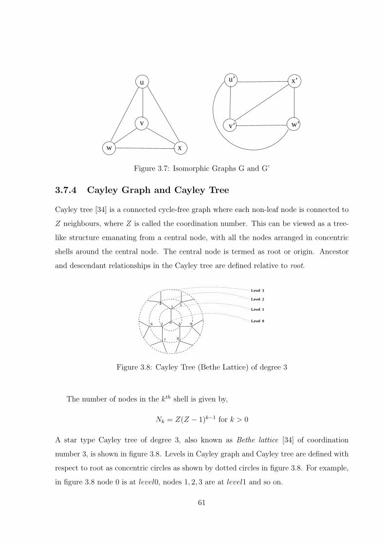
x

u

v

u’

v’

x’

w’

w

Figure 3.7: Isomorphic Graphs G and G’

3.7.4 Cayley Graph and Cayley Tree

Cayley tree [34] is a connected cycle-free graph where each non-leaf node is connected to

Z neighbours, where Z is called the coordination number. This can be viewed as a tree-

like structure emanating from a central node, with all the nodes arranged in concentric

shells around the central node. The central node is termed as root or origin. Ancestor

and descendant relationships in the Cayley tree are defined relative to root.

7

Level 2

Level 3

Level 1

Level 0o

1

2 3 96

4 5

8

Figure 3.8: Cayley Tree (Bethe Lattice) of degree 3

The number of nodes in the kth shell is given by,

Nk = Z(Z − 1)k−1 for k > 0

A star type Cayley tree of degree 3, also known as Bethe lattice [34] of coordination

number 3, is shown in figure 3.8. Levels in Cayley graph and Cayley tree are defined with

respect to root as concentric circles as shown by dotted circles in figure 3.8. For example,

in figure 3.8 node 0 is at level0, nodes 1, 2, 3 are at level1 and so on.

61

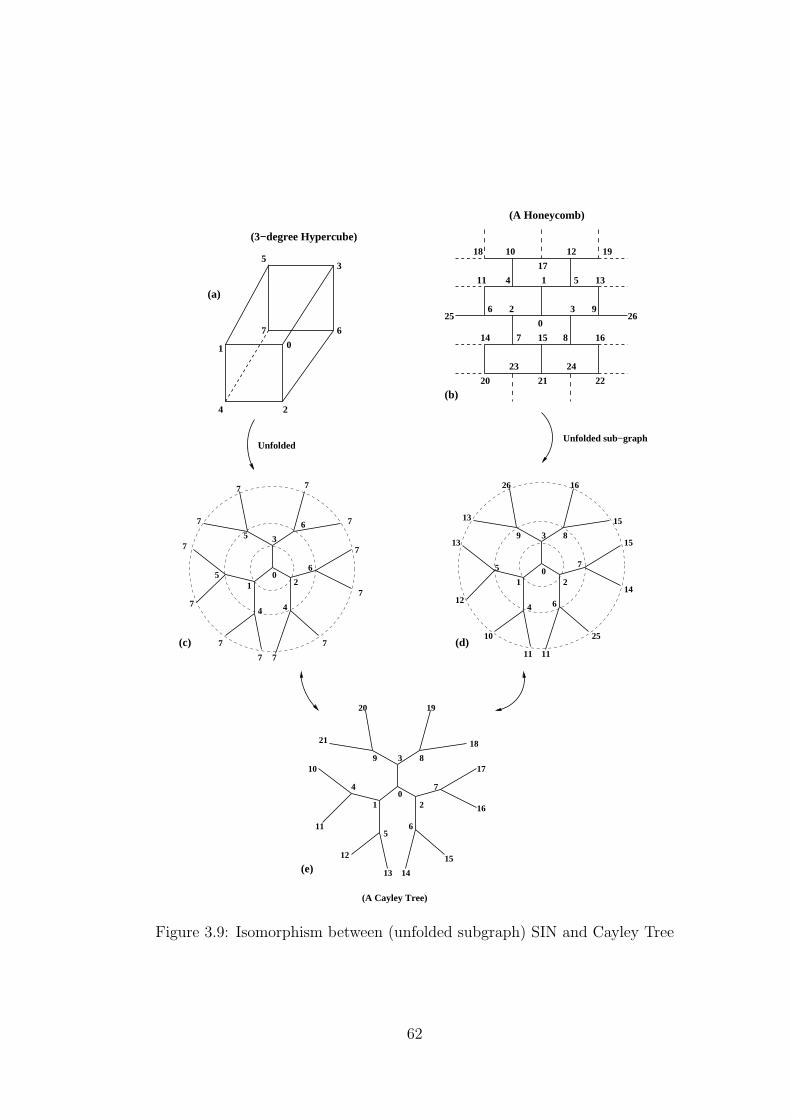
(a)

01 2

3

6

7

89

4

5

10

12

15

15

14

11 11

16

13

13

25

26

01

2

3

4

5

670

1

2 3

54

6

7 8

9

10

11

12

13

14 15 16

17

1918

20 21 22

23 24

01 2

3

6

4

7

7

7

7

7

7 7

7

7

7

7

7

25 26

01 2

3

6

7

89

1821

20

5

4

10

11

12

13

15

14

16

17

19

(3−degree Hypercube)

(A Honeycomb)

UnfoldedUnfolded sub−graph

(A Cayley Tree)

4

56

5

(b)

(c) (d)

(e)

Figure 3.9: Isomorphism between (unfolded subgraph) SIN and Cayley Tree

62

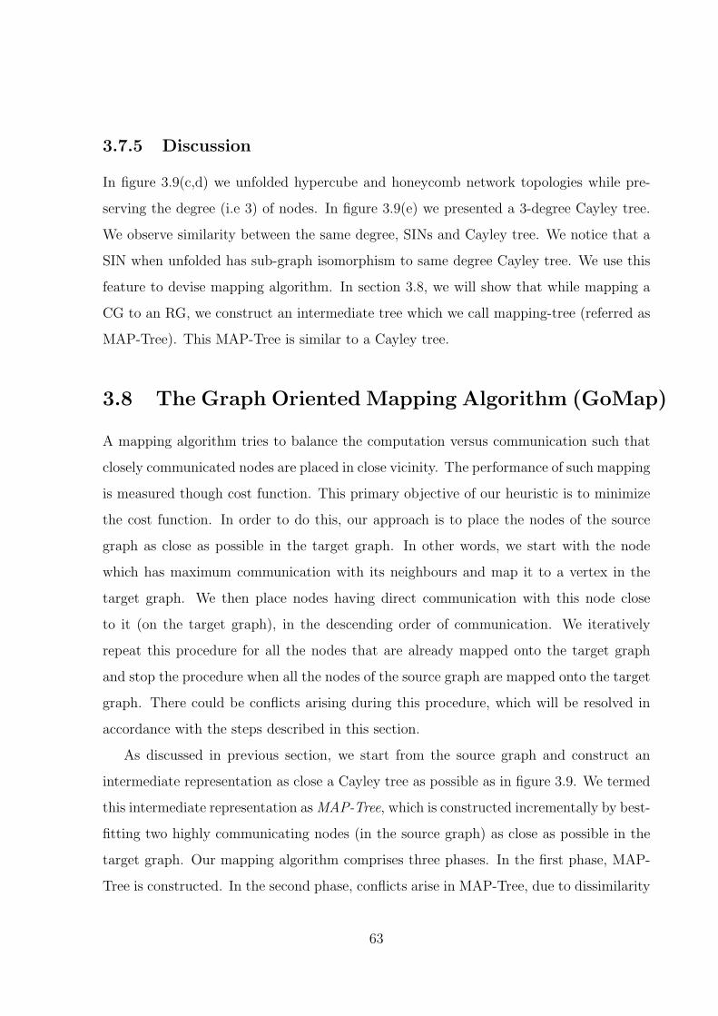
3.7.5 Discussion

In figure 3.9(c,d) we unfolded hypercube and honeycomb network topologies while pre-

serving the degree (i.e 3) of nodes. In figure 3.9(e) we presented a 3-degree Cayley tree.

We observe similarity between the same degree, SINs and Cayley tree. We notice that a

SIN when unfolded has sub-graph isomorphism to same degree Cayley tree. We use this

feature to devise mapping algorithm. In section 3.8, we will show that while mapping a

CG to an RG, we construct an intermediate tree which we call mapping-tree (referred as

MAP-Tree). This MAP-Tree is similar to a Cayley tree.

3.8 The Graph Oriented Mapping Algorithm (GoMap)

A mapping algorithm tries to balance the computation versus communication such that

closely communicated nodes are placed in close vicinity. The performance of such mapping

is measured though cost function. This primary objective of our heuristic is to minimize

the cost function. In order to do this, our approach is to place the nodes of the source

graph as close as possible in the target graph. In other words, we start with the node

which has maximum communication with its neighbours and map it to a vertex in the

target graph. We then place nodes having direct communication with this node close

to it (on the target graph), in the descending order of communication. We iteratively

repeat this procedure for all the nodes that are already mapped onto the target graph

and stop the procedure when all the nodes of the source graph are mapped onto the target

graph. There could be conflicts arising during this procedure, which will be resolved in

accordance with the steps described in this section.

As discussed in previous section, we start from the source graph and construct an

intermediate representation as close a Cayley tree as possible as in figure 3.9. We termed

this intermediate representation asMAP-Tree, which is constructed incrementally by best-

fitting two highly communicating nodes (in the source graph) as close as possible in the

target graph. Our mapping algorithm comprises three phases. In the first phase, MAP-

Tree is constructed. In the second phase, conflicts arise in MAP-Tree, due to dissimilarity

63

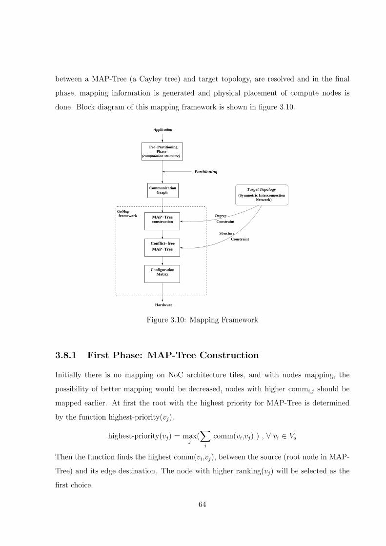
between a MAP-Tree (a Cayley tree) and target topology, are resolved and in the final

phase, mapping information is generated and physical placement of compute nodes is

done. Block diagram of this mapping framework is shown in figure 3.10.

PhasePre−Partitioning

Communication Graph

Application

Degree

Constraint

Structure

Constraint

MAP−Tree

MAP−Tree

ConfigurationMatrix

construction

Partitioning

(computation structure)

Hardware

GoMapframework

Conflict−free

(Symmetric Interconnection

Target Topology

Network)

Figure 3.10: Mapping Framework

3.8.1 First Phase: MAP-Tree Construction

Initially there is no mapping on NoC architecture tiles, and with nodes mapping, the

possibility of better mapping would be decreased, nodes with higher commi,j should be

mapped earlier. At first the root with the highest priority for MAP-Tree is determined

by the function highest-priority(vj).

highest-priority(vj) = maxj

(∑

i

comm(vi,vj) ) , ∀ vi ∈ Vs

Then the function finds the highest comm(vi,vj), between the source (root node in MAP-

Tree) and its edge destination. The node with higher ranking(vj) will be selected as the

first choice.

64

Ranking(vj) = maxj

(comm(vi,vj) ) , ∀ vi ∈ MAP-Tree and ∀ vj /∈ MAP-Tree

We iteratively calculate the Ranking of each vj(∈ Vs) and not in MAP-Tree with respect

to the nodes vi ∈ MAP-Tree and incrementally add the selected vj in MAP-Tree with

the edge(vi,vj). If degree of vi is k i.e. max degree of MAP-Tree, we select the descen-

dants(n,m) of vi and compute sum of remaining communications, which have not been

considered for MAP-Tree, individually for both n and m. Select node with lower sum

under constraint degree[selected node] < k. If constraint not fulfilled, repeat for other

node. If none applies iterate this until we find one descendant node (say p). Then we add

vj with edge(p,vj). We repeat this for each node vj in source graph Gs(Vs,Es) that are

not in MAP-Tree. Pseudo code for MAP-Tree construction is given in Algorithm 4.

3.8.2 Second Phase : MAP-Tree Conflict Check and Resolution

After constructing MAP-Tree (lets say degree 3) as aforesaid methodology, we get MAP-

Tree similar to figure 3.8 or figure 3.9(e). This MAP-Tree doesn’t ensure an embedding

for the target graph. This depends on the size of MAP-Tree as well the degree and

structure of target graph. The ”conflict” could occur in this MAP-Tree. Conflict is the

case, where two or more nodes of MAP-Tree contend for the same node of NoC. The sole

basis of conflict is: consideration of independent child node in MAP-Tree construction

with contradiction to shared child node in target graph due to merger of some nodes in

later. See figure 3.9 for an illustration of the same. Difference in these two gets to appear

only after, if MAP-Tree has at-least certain nodes (see figure 3.9) which varies as per the

degree as well structural constraint (refer c,d of figure 3.9) of target graph.

Resolution: Conflict occurs because of mapping t nodes in t − 1 or lesser, positions

available, so conflict resolution has been made by moving ”one” among conflicted node as

a descendant to it’s parent descendants from the highest level of conflict. For example in

hypercube topology, conflict will start occurring only at level 2 or more. Least commu-

nicative node has been chosen and associated as a descendant, of its parent (immediate

ancestor) immediate descendant. Once all the ”nodes in conflict” are made conflict-free

at one level, we move to level beneath and check for state of conflict for all the nodes

65

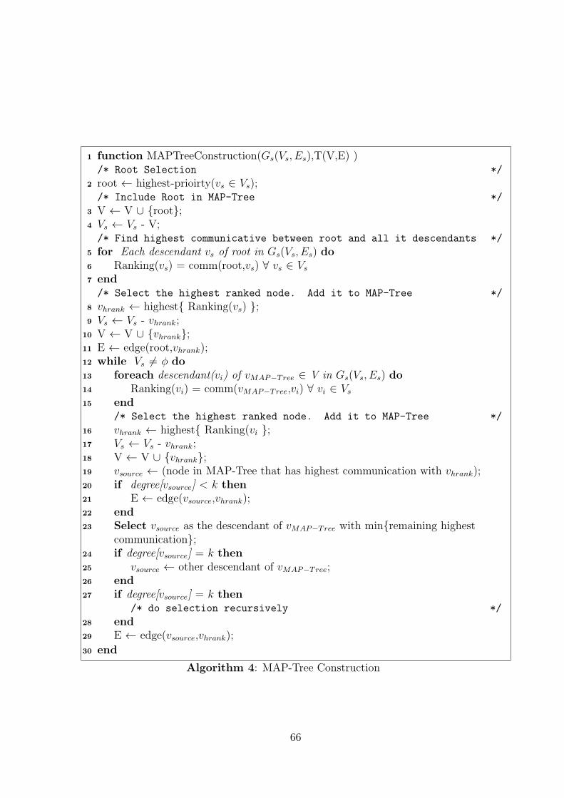
function MAPTreeConstruction(Gs(Vs, Es),T(V,E) )1

/* Root Selection */

root ← highest-prioirty(vs ∈ Vs);2

/* Include Root in MAP-Tree */

V ← V ∪ {root};3

Vs ← Vs - V;4

/* Find highest communicative between root and all it descendants */

for Each descendant vs of root in Gs(Vs, Es) do5

Ranking(vs) = comm(root,vs) ∀ vs ∈ Vs6

end7

/* Select the highest ranked node. Add it to MAP-Tree */

vhrank ← highest{ Ranking(vs) };8

Vs ← Vs - vhrank;9

V ← V ∪ {vhrank};10

E ← edge(root,vhrank);11

while Vs 6= φ do12

foreach descendant(vi) of vMAP−Tree ∈ V in Gs(Vs, Es) do13

Ranking(vi) = comm(vMAP−Tree,vi) ∀ vi ∈ Vs14

end15

/* Select the highest ranked node. Add it to MAP-Tree */

vhrank ← highest{ Ranking(vi };16

Vs ← Vs - vhrank;17

V ← V ∪ {vhrank};18

vsource ← (node in MAP-Tree that has highest communication with vhrank);19

if degree[vsource] < k then20

E ← edge(vsource,vhrank);21

end22

Select vsource as the descendant of vMAP−Tree with min{remaining highest23

communication};if degree[vsource] = k then24

vsource ← other descendant of vMAP−Tree;25

end26

if degree[vsource] = k then27

/* do selection recursively */

end28

E ← edge(vsource,vhrank);29

end30

Algorithm 4: MAP-Tree Construction

66

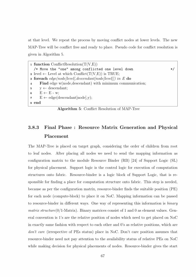
at that level. We repeat the process by moving conflict nodes at lower levels. The new

MAP-Tree will be conflict free and ready to place. Pseudo code for conflict resolution is

given in Algorithm 5.

function ConflictResolution(T(V,E))1

/* Move the "one" among conflicted one level down */

level ← Level at which Conflict(T(V,E)) is TRUE;2

foreach edge(node[level],descendant[node[level]]) in E do3

Find edge w(node,descendant) with minimum communication;4

y ← descendant;5

E ← E - w;6

E ← edge(descendant[node],y);7

end8

Algorithm 5: Conflict Resolution of MAP-Tree

3.8.3 Final Phase : Resource Matrix Generation and Physical

Placement

The MAP-Tree is placed on target graph, considering the order of children from root

to leaf nodes. After placing all nodes we need to send the mapping information as

configuration matrix to the module Resource Binder (RB) [24] of Support Logic (SL)

for physical placement. Support logic is the control logic for execution of computation

structures onto fabric. Resource-binder is a logic block of Support Logic, that is re-

sponsible for finding a place for computation structure onto fabric. This step is needed,

because as per the configuration matrix, resource-binder finds the suitable position (PE)

for each node (compute-block) to place it on NoC. Mapping information can be passed

to resource-binder in different ways. One way of representing this information is binary

matrix structure(0/1-Matrix). Binary matrices consist of 1 and 0 as element values. Gen-

eral convention is 1’s are the relative position of nodes which need to get placed on NoC

in exactly same fashion with respect to each other and 0’s as relative positions, which are

don’t care (irrespective of PEs status) place in NoC. Don’t care position assumes that

resource-binder need not pay attention to the availability status of relative PEs on NoC

while making decision for physical placements of nodes. Resource-binder gives the start

67

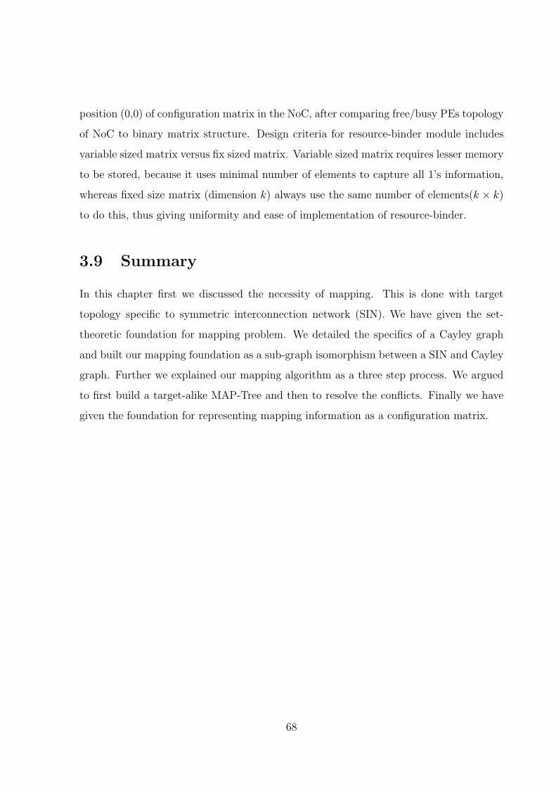
position (0,0) of configuration matrix in the NoC, after comparing free/busy PEs topology

of NoC to binary matrix structure. Design criteria for resource-binder module includes

variable sized matrix versus fix sized matrix. Variable sized matrix requires lesser memory

to be stored, because it uses minimal number of elements to capture all 1’s information,

whereas fixed size matrix (dimension k) always use the same number of elements(k × k)

to do this, thus giving uniformity and ease of implementation of resource-binder.

3.9 Summary

In this chapter first we discussed the necessity of mapping. This is done with target

topology specific to symmetric interconnection network (SIN). We have given the set-

theoretic foundation for mapping problem. We detailed the specifics of a Cayley graph

and built our mapping foundation as a sub-graph isomorphism between a SIN and Cayley

graph. Further we explained our mapping algorithm as a three step process. We argued

to first build a target-alike MAP-Tree and then to resolve the conflicts. Finally we have

given the foundation for representing mapping information as a configuration matrix.

68

Chapter 4

Mapping Case-Study

In this chapter we apply our mapping algorithm GoMap with specifics to honeycomb

and mesh networks. We discuss the properties of these two network topologies. We also

discuss the challenges involved in mapping with respect to these target graphs.

Rest of the chapter is organised as follows. In section 4.1 we revisit the key features

of a symmetric interconnection network (SIN). In section 4.2 we give the characteristic

of a honeycomb network and explore the mapping prospects on it. Section 4.3 details

our mapping algorithm GoMap with honeycomb as target topology. In section 4.4 we

illustrate mapping through an example. In section 4.5 we bring the discussion on mesh

topology and provide the characteristics of a mesh. Section 4.6 give details of mapping

on a mesh topology.

4.1 Symmetric Interconnection Network (SIN): A Re-

visit

In previous chapter we discussed various parameters for designing of a network. In this sec-

tion we focus on a special class of networks called as symmetric interconnection networks

(SINs). SINs are widely popular as preferred choice for network topology importantly due

to following two features:

69

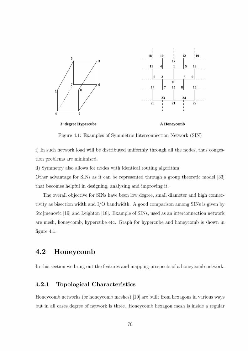
A Honeycomb

01

2

3

4

5

670

1

2 3

54

6

7 8

9

10

11

12

13

14 15 16

17

1918

20 21 22

23 24

3−degree Hypercube

Figure 4.1: Examples of Symmetric Interconnection Network (SIN)

i) In such network load will be distributed uniformly through all the nodes, thus conges-

tion problems are minimized.

ii) Symmetry also allows for nodes with identical routing algorithm.

Other advantage for SINs as it can be represented through a group theoretic model [33]

that becomes helpful in designing, analysing and improving it.

The overall objective for SINs have been low degree, small diameter and high connec-

tivity as bisection width and I/O bandwidth. A good comparison among SINs is given by

Stojmenovic [19] and Leighton [18]. Example of SINs, used as an interconnection network

are mesh, honeycomb, hypercube etc. Graph for hypercube and honeycomb is shown in

figure 4.1.

4.2 Honeycomb

In this section we bring out the features and mapping prospects of a honeycomb network.

4.2.1 Topological Characteristics

Honeycomb networks (or honeycomb meshes) [19] are built from hexagons in various ways

but in all cases degree of network is three. Honeycomb hexagon mesh is inside a regular

70

hexagon (refer figure 3.3 ). For a honeycomb, diameter is 1.63√n and bisection width is

0.82√n [19]. Our target topology is a toroidal honeycomb mesh [24] but we will refer

this as honeycomb. Also, without loss of generalisation, in diagrams we are referring

only a part of a complete honeycomb network. Honeycomb has been studied in detail by

Stojmenovic [19].

4.2.2 Honeycomb as a Cayley Graph

As mentioned in section 3.7, honeycomb topology is a Cayley graph [33] of degree 3 and

is a graph having the following property:

i) root node (node 0 in Fig. 4.3) at center with three edges emanating from the it,

ii) for all nodes, that are independent (only one immediate ancestor) children (node 1,2),

two edges emanate from that node,

iii) for all other nodes that are shared (two immediate ancestors) children (node 10,13),

only one edge emanate from that node,

iv) there exists cycles of length 6 nodes and every node of a cycle is part of two other

different cycles of length 6.

Property (i) and (ii), gives the basis for construction of Cayley tree of degree 3. From

this we deduce that, in a honeycomb, if we relax property (iii) and (iv) among nodes

(refer figure 4.2), then Cayley tree data structure can be applied for the purpose of

mapping onto honeycomb. Refer figure 4.3 for an illustartion of the same. We will use

this basis for mapping formulation of honeycomb. With this basis we go in detail of our

mapping formulation. We will discuss relaxation of (iii) and (iv) (4.6.2) while discussing

the mapping.

4.3 Mapping onto Honeycomb

Approach is to start from the source graph and construct an intermediate representation

as close a Cayley tree as possible. We term this intermediate representation as MAP-

Tree, which is constructed incrementally by best-fitting two highly communicating nodes

71

(A Cayley Tree)

01 2

3

6

7

89

1821

20

5

4

10

11

12

13

15

14

16

17

19

(b)

(c)

0

1

2 3

54

6

7 8

9

10

11

12

13

14 15 16

17

1918

20 21 22

23 24

25 26

(a)

01 2

3

6

7

89

4

5

10

12

15

15

14

11 11

16

13

13

25

26

(A Honeycomb) (Unfolded sub−graph)

Figure 4.2: Isomorphism between Honeycomb (un-folded) and Cayley Tree

(in the source graph) as close as possible in the target graph. Our mapping algorithm

comprises three phases. In the first phase, a 3-degree Cayley Tree is constructed as MAP-

Tree. In the second phase, conflicts arise in MAP-Tree, due to relaxation of property (iii)

and (iv) (see section 4.2.2) of Cayley graph, are resolved and in the final phase, mapping

information is generated and physical placement of compute nodes is done.

4.3.1 MAP-Tree Construction

As we map the nodes, the possibility of better mapping would be decreased so nodes with

higher commi,j should be mapped earlier. At first the root with the highest priority for

MAP-Tree is determined by the function highest-priority(vj). Then the function finds

the highest comm(vi,vj), between the source vi (root node in MAP-Tree) and its edge

destination vj. The node with higher ranking(vj) will be selected as the first choice. We

iteratively calculate the ranking of each vj that is in source graph but not in MAP-Tree

with respect to the nodes vi that are in MAP-Tree and incrementally add the selected

72

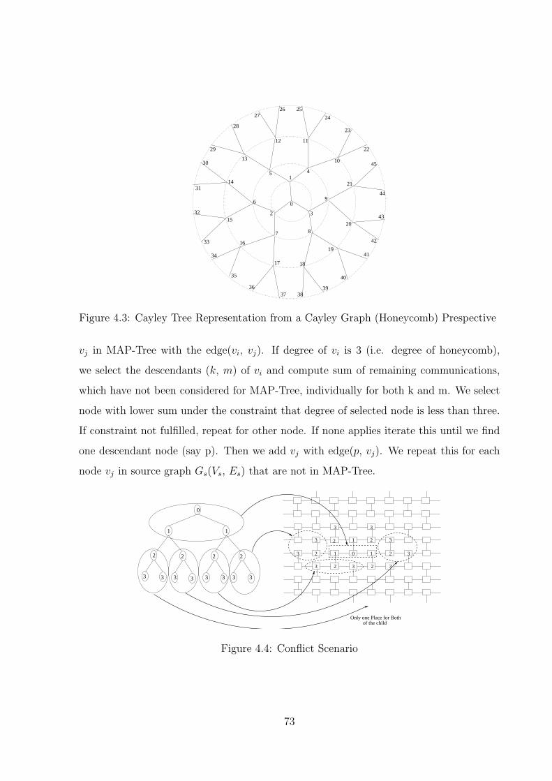
3

6

7

25

0

2

145

8

9

1112

15

16

17 18

19

20

21

10

23

24

2627

28

29

30

31

32

14

13

33

34

35

3637 38

39

40

41

42

43

44

45

22

Figure 4.3: Cayley Tree Representation from a Cayley Graph (Honeycomb) Prespective

vj in MAP-Tree with the edge(vi, vj). If degree of vi is 3 (i.e. degree of honeycomb),

we select the descendants (k, m) of vi and compute sum of remaining communications,

which have not been considered for MAP-Tree, individually for both k and m. We select

node with lower sum under the constraint that degree of selected node is less than three.

If constraint not fulfilled, repeat for other node. If none applies iterate this until we find

one descendant node (say p). Then we add vj with edge(p, vj). We repeat this for each

node vj in source graph Gs(Vs, Es) that are not in MAP-Tree.

01

1

12

2

2 2

2

2

3

3

3 3

3 3

3

3

3

0

1 1

2 2 2 2

3 3 3 3 3 3 3 3

Only one Place for Bothof the child

Figure 4.4: Conflict Scenario

73

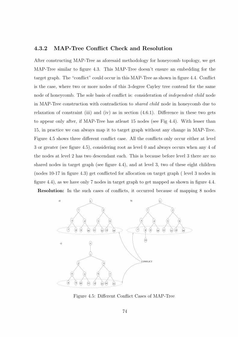
4.3.2 MAP-Tree Conflict Check and Resolution

After constructing MAP-Tree as aforesaid methodology for honeycomb topology, we get

MAP-Tree similar to figure 4.3. This MAP-Tree doesn’t ensure an embedding for the

target graph. The “conflict” could occur in this MAP-Tree as shown in figure 4.4. Conflict

is the case, where two or more nodes of this 3-degree Cayley tree contend for the same

node of honeycomb. The sole basis of conflict is: consideration of independent child node

in MAP-Tree construction with contradiction to shared child node in honeycomb due to

relaxation of constraint (iii) and (iv) as in section (4.6.1). Difference in these two gets

to appear only after, if MAP-Tree has atleast 15 nodes (see Fig 4.4). With lesser than

15, in practice we can always map it to target graph without any change in MAP-Tree.

Figure 4.5 shows three different conflict case. All the conflicts only occur either at level

3 or greater (see figure 4.5), considering root as level 0 and always occurs when any 4 of

the nodes at level 2 has two descendant each. This is because before level 3 there are no

shared nodes in target graph (see figure 4.4), and at level 3, two of these eight children

(nodes 10-17 in figure 4.3) get conflicted for allocation on target graph ( level 3 nodes in

figure 4.4), as we have only 7 nodes in target graph to get mapped as shown in figure 4.4.

Resolution: In the such cases of conflicts, it occurred because of mapping 8 nodes

7

0

1 2

3 4 5 6

7 8 9 10 11 12 13 14

0

1 2

3 4 5 6

7 8 9 10 11 12 13 14

15

CONFLICT

a) b)

0

1

2 3

4 5 6

8 9 10 11 12 13 14 15

c)

Figure 4.5: Different Conflict Cases of MAP-Tree

74

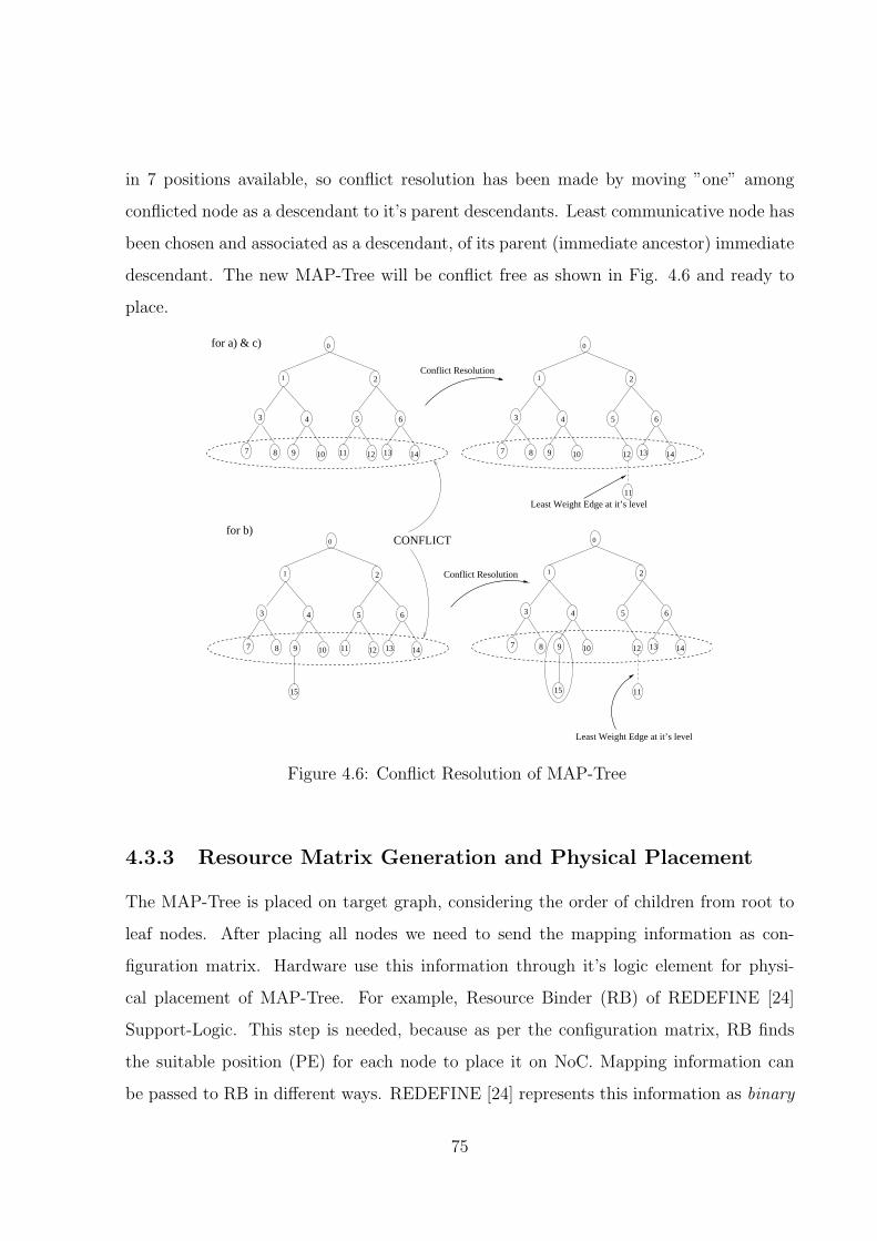
in 7 positions available, so conflict resolution has been made by moving ”one” among

conflicted node as a descendant to it’s parent descendants. Least communicative node has

been chosen and associated as a descendant, of its parent (immediate ancestor) immediate

descendant. The new MAP-Tree will be conflict free as shown in Fig. 4.6 and ready to

place.

0

1 2

3 4 5 6

7 8 9 10 11 12 13 14

for a) & c) 0

1 2

3 4 5 6

7 8 9 10 12 13 14

Conflict Resolution

11

for b)0

1 2

3 4 5 6

7 8 9 10 12 13 14

15

CONFLICT0

1 2

3 4 5 6

7 8 9 10 11 12 13 14

15

Conflict Resolution

11

Least Weight Edge at it’s level

Least Weight Edge at it’s level

Figure 4.6: Conflict Resolution of MAP-Tree

4.3.3 Resource Matrix Generation and Physical Placement

The MAP-Tree is placed on target graph, considering the order of children from root to

leaf nodes. After placing all nodes we need to send the mapping information as con-

figuration matrix. Hardware use this information through it’s logic element for physi-

cal placement of MAP-Tree. For example, Resource Binder (RB) of REDEFINE [24]

Support-Logic. This step is needed, because as per the configuration matrix, RB finds

the suitable position (PE) for each node to place it on NoC. Mapping information can

be passed to RB in different ways. REDEFINE [24] represents this information as binary

75

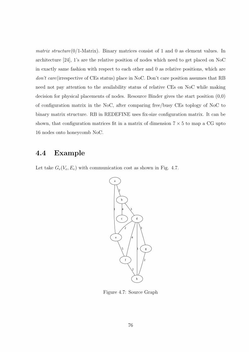
matrix structure(0/1-Matrix). Binary matrices consist of 1 and 0 as element values. In

architecture [24], 1’s are the relative position of nodes which need to get placed on NoC

in exactly same fashion with respect to each other and 0 as relative positions, which are

don’t care(irrespective of CEs status) place in NoC. Don’t care position assumes that RB

need not pay attention to the availability status of relative CEs on NoC while making

decision for physical placements of nodes. Resource Binder gives the start position (0,0)

of configuration matrix in the NoC, after comparing free/busy CEs toplogy of NoC to

binary matrix structure. RB in REDEFINE uses fix-size configuration matrix. It can be

shown, that configuration matrices fit in a matrix of dimension 7× 5 to map a CG upto

16 nodes onto honeycomb NoC.

4.4 Example

Let take Ge(Ve, Ee) with communication cost as shown in Fig. 4.7.

a

b

2

e

1

c

4

d

3

2

f

4

g

3

h

15

2

2

Figure 4.7: Source Graph

76

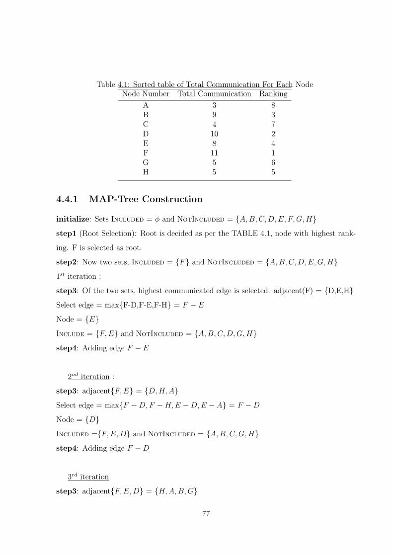
Table 4.1: Sorted table of Total Communication For Each NodeNode Number Total Communication Ranking

A 3 8B 9 3C 4 7D 10 2E 8 4F 11 1G 5 6H 5 5

4.4.1 MAP-Tree Construction

initialize: Sets Included = φ and NotIncluded = {A,B,C,D,E, F,G,H}step1 (Root Selection): Root is decided as per the TABLE 4.1, node with highest rank-

ing. F is selected as root.

step2: Now two sets, Included = {F} and NotIncluded = {A,B,C,D,E,G,H}1st iteration :

step3: Of the two sets, highest communicated edge is selected. adjacent(F) = {D,E,H}Select edge = max{F-D,F-E,F-H} = F − E

Node = {E}Include = {F,E} and NotIncluded = {A,B,C,D,G,H}step4: Adding edge F − E

2nd iteration :

step3: adjacent{F,E} = {D,H,A}Select edge = max{F −D,F −H,E −D,E − A} = F −D

Node = {D}Included ={F,E,D} and NotIncluded = {A,B,C,G,H}step4: Adding edge F −D

3rd iteration

step3: adjacent{F,E,D} = {H,A,B,G}

77

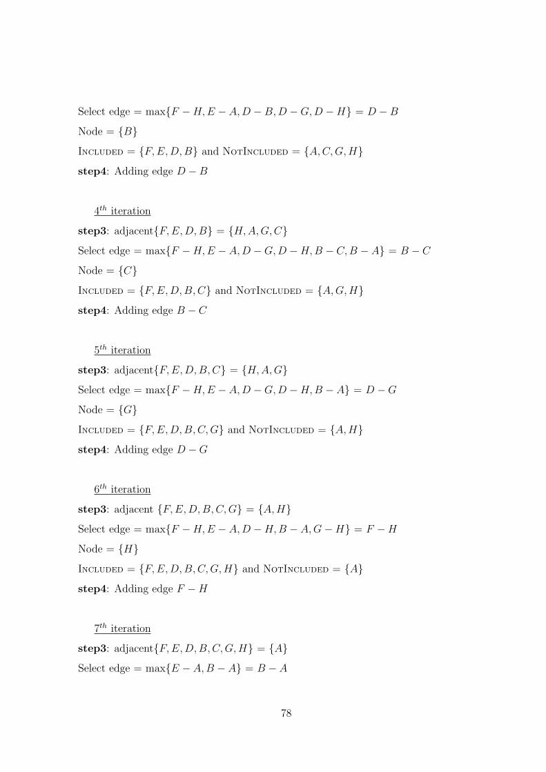
Select edge = max{F −H,E − A,D −B,D −G,D −H} = D − B

Node = {B}Included = {F,E,D,B} and NotIncluded = {A,C,G,H}step4: Adding edge D −B

4th iteration

step3: adjacent{F,E,D,B} = {H,A,G,C}Select edge = max{F −H,E − A,D −G,D −H,B − C,B − A} = B − C

Node = {C}Included = {F,E,D,B,C} and NotIncluded = {A,G,H}step4: Adding edge B − C

5th iteration

step3: adjacent{F,E,D,B,C} = {H,A,G}Select edge = max{F −H,E − A,D −G,D −H,B − A} = D −G

Node = {G}Included = {F,E,D,B,C,G} and NotIncluded = {A,H}step4: Adding edge D −G

6th iteration

step3: adjacent {F,E,D,B,C,G} = {A,H}Select edge = max{F −H,E − A,D −H,B − A,G−H} = F −H

Node = {H}Included = {F,E,D,B,C,G,H} and NotIncluded = {A}step4: Adding edge F −H

7th iteration

step3: adjacent{F,E,D,B,C,G,H} = {A}Select edge = max{E − A,B − A} = B − A

78

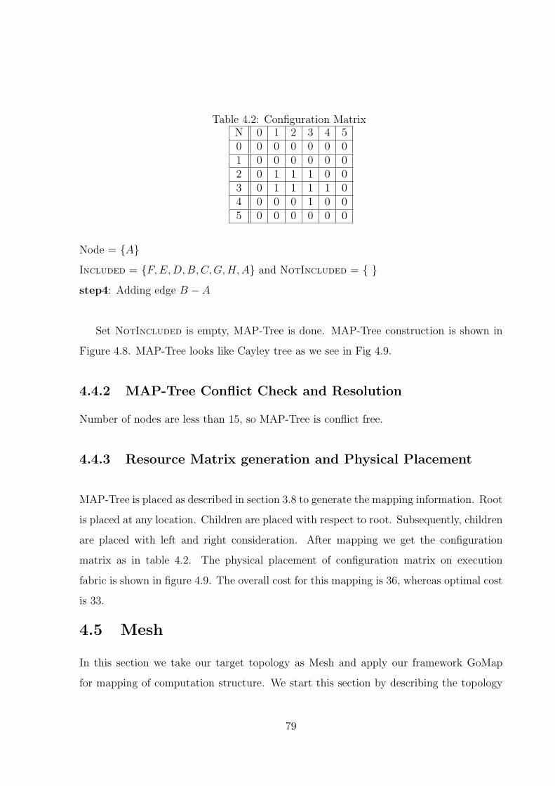
Table 4.2: Configuration MatrixN 0 1 2 3 4 50 0 0 0 0 0 01 0 0 0 0 0 02 0 1 1 1 0 03 0 1 1 1 1 04 0 0 0 1 0 05 0 0 0 0 0 0

Node = {A}Included = {F,E,D,B,C,G,H,A} and NotIncluded = { }step4: Adding edge B − A

Set NotIncluded is empty, MAP-Tree is done. MAP-Tree construction is shown in

Figure 4.8. MAP-Tree looks like Cayley tree as we see in Fig 4.9.

4.4.2 MAP-Tree Conflict Check and Resolution

Number of nodes are less than 15, so MAP-Tree is conflict free.

4.4.3 Resource Matrix generation and Physical Placement

MAP-Tree is placed as described in section 3.8 to generate the mapping information. Root

is placed at any location. Children are placed with respect to root. Subsequently, children

are placed with left and right consideration. After mapping we get the configuration

matrix as in table 4.2. The physical placement of configuration matrix on execution

fabric is shown in figure 4.9. The overall cost for this mapping is 36, whereas optimal cost

is 33.

4.5 Mesh

In this section we take our target topology as Mesh and apply our framework GoMap

for mapping of computation structure. We start this section by describing the topology

79

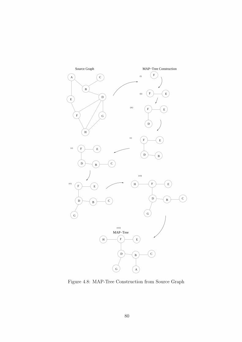
ED

B

C

G

H

CB D

F E

G

A

A

F

(i)

(ii)

(iii)

iv)

(v)

(vii)

(viii)

F E

D B C

H F

D

G

B

E

C

B D

F E

H

D

F E

EF

F

(vi)

F E

D

G

B C

Source Graph MAP−Tree Construction

MAP−Tree

Figure 4.8: MAP-Tree Construction from Source Graph

80

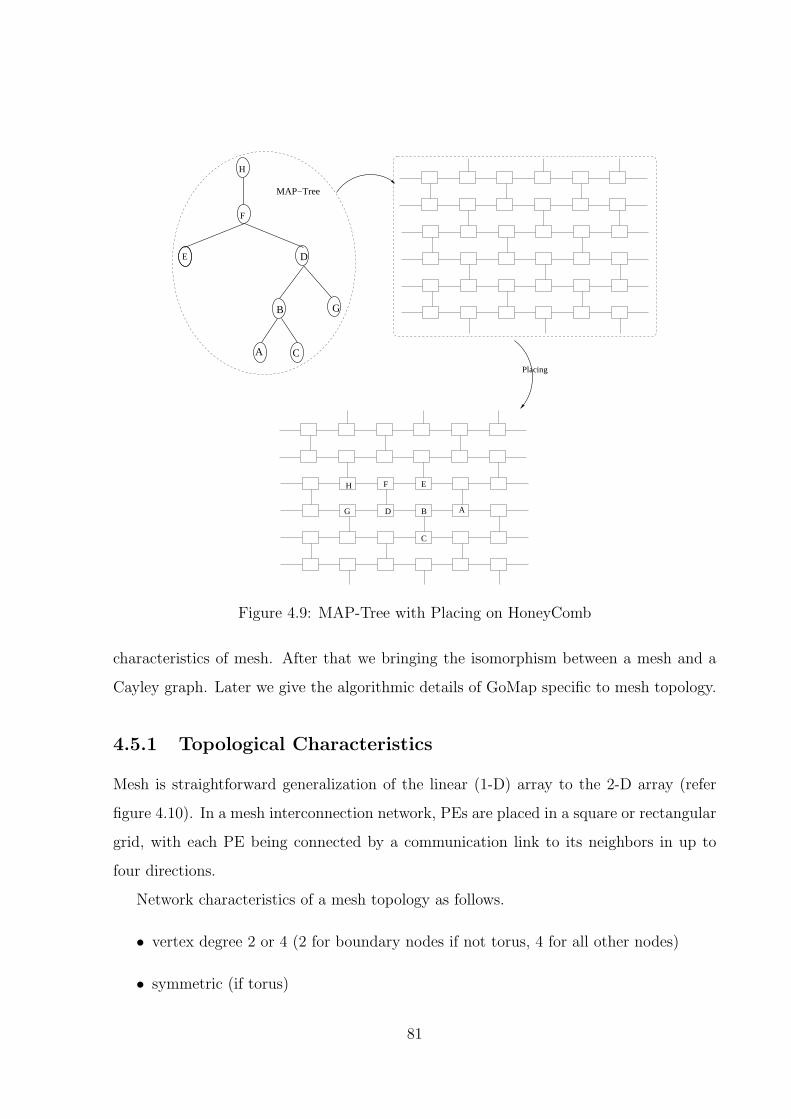
F

CA

E

H

B

D

G

MAP−Tree

Placing

F

AB

C

DG

H E

Figure 4.9: MAP-Tree with Placing on HoneyComb

characteristics of mesh. After that we bringing the isomorphism between a mesh and a

Cayley graph. Later we give the algorithmic details of GoMap specific to mesh topology.

4.5.1 Topological Characteristics

Mesh is straightforward generalization of the linear (1-D) array to the 2-D array (refer

figure 4.10). In a mesh interconnection network, PEs are placed in a square or rectangular

grid, with each PE being connected by a communication link to its neighbors in up to

four directions.

Network characteristics of a mesh topology as follows.

• vertex degree 2 or 4 (2 for boundary nodes if not torus, 4 for all other nodes)

• symmetric (if torus)

81

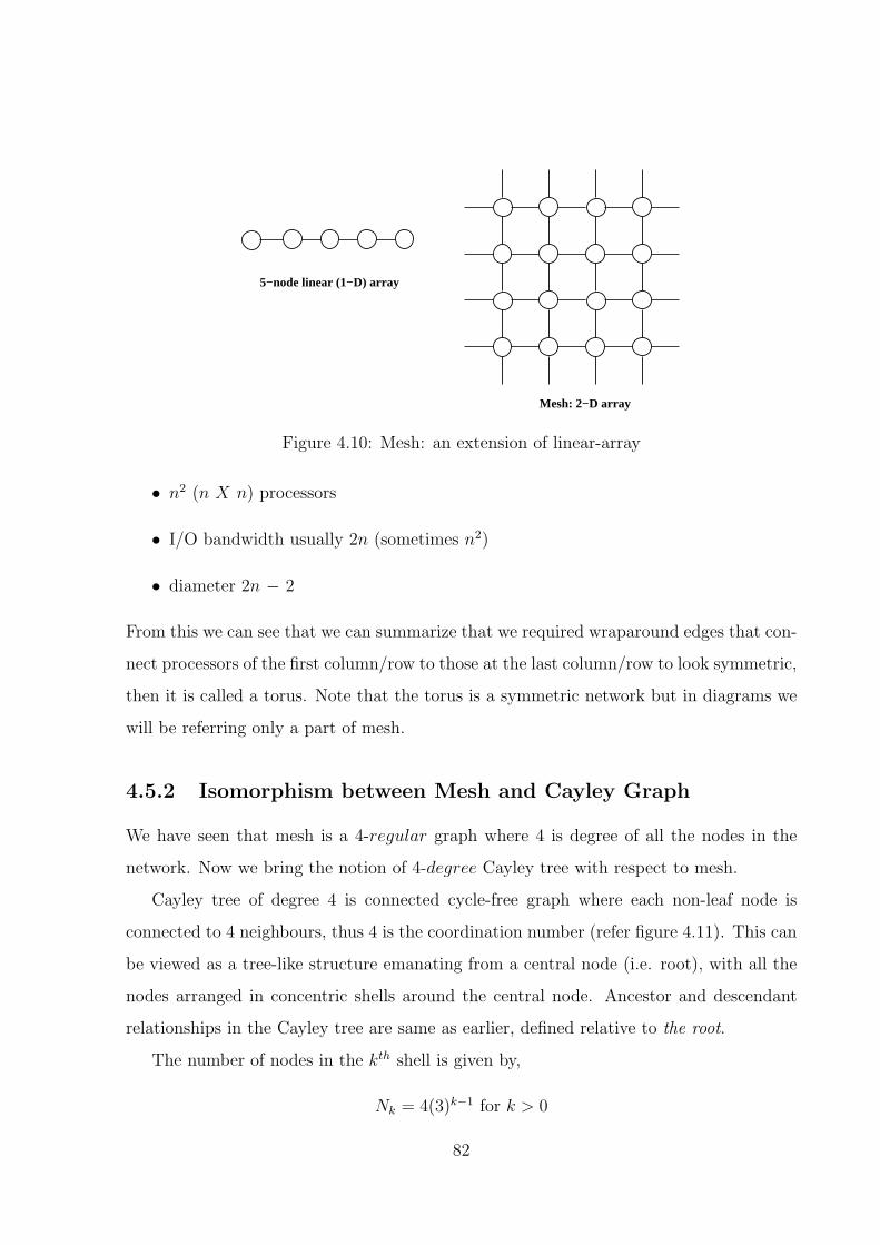
5−node linear (1−D) array

Mesh: 2−D array

Figure 4.10: Mesh: an extension of linear-array

• n2 (n X n) processors

• I/O bandwidth usually 2n (sometimes n2)

• diameter 2n − 2

From this we can see that we can summarize that we required wraparound edges that con-

nect processors of the first column/row to those at the last column/row to look symmetric,

then it is called a torus. Note that the torus is a symmetric network but in diagrams we

will be referring only a part of mesh.

4.5.2 Isomorphism between Mesh and Cayley Graph

We have seen that mesh is a 4-regular graph where 4 is degree of all the nodes in the

network. Now we bring the notion of 4-degree Cayley tree with respect to mesh.

Cayley tree of degree 4 is connected cycle-free graph where each non-leaf node is

connected to 4 neighbours, thus 4 is the coordination number (refer figure 4.11). This can

be viewed as a tree-like structure emanating from a central node (i.e. root), with all the

nodes arranged in concentric shells around the central node. Ancestor and descendant

relationships in the Cayley tree are same as earlier, defined relative to the root.

The number of nodes in the kth shell is given by,

Nk = 4(3)k−1 for k > 0

82

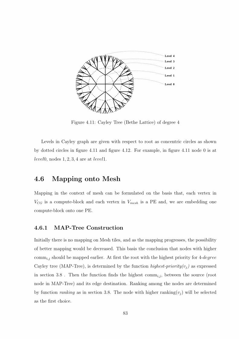
Level 0

Level 2

Level 3

Level 4

Level 1

Figure 4.11: Cayley Tree (Bethe Lattice) of degree 4

Levels in Cayley graph are given with respect to root as concentric circles as shown

by dotted circles in figure 4.11 and figure 4.12. For example, in figure 4.11 node 0 is at

level0, nodes 1, 2, 3, 4 are at level1.

4.6 Mapping onto Mesh

Mapping in the context of mesh can be formulated on the basis that, each vertex in

VCG is a compute-block and each vertex in Vmesh is a PE and, we are embedding one

compute-block onto one PE.

4.6.1 MAP-Tree Construction

Initially there is no mapping on Mesh tiles, and as the mapping progresses, the possibility

of better mapping would be decreased. This basis the conclusion that nodes with higher

commi,j should be mapped earlier. At first the root with the highest priority for 4-degree

Cayley tree (MAP-Tree), is determined by the function highest-priority(vj) as expressed

in section 3.8 . Then the function finds the highest commi,j , between the source (root

node in MAP-Tree) and its edge destination. Ranking among the nodes are determined

by function ranking as in section 3.8. The node with higher ranking(vj) will be selected

as the first choice.

83

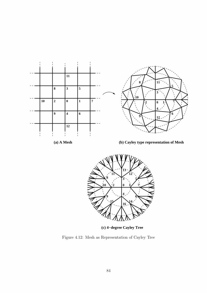
(c) 4−degree Cayley Tree

0 12

3

4

5

6

7

8

9

10

11

12

0 12

3

4

5

6

7

8

9

10

11

12

0 12

3

4

5

6

7

8

9

10

11 1213

141516

(b) Cayley type representation of Mesh(a) A Mesh

Figure 4.12: Mesh as Representation of Cayley Tree

84

We iteratively calculate the ranking of each vj in computation structure (i.e. ∈ Vs)

and not in MAP-Tree with respect to the nodes vi ∈ MAP-Tree and incrementally add

the selected vj in MAP-Tree with the edge(vi, vj). If degree of vi is 4, we select the

descendants(k, l, m) of vi and compute sum of remaining communications, which have

not been considered for MAP-Tree, individually for all k, l and m. Select node with lower

sum under constraint degree[selected node] < 4. If constraint not fulfilled, repeat for

other node. If none applies iterate this until we find one descendant node (say p). Then

we add vj with edge(p, vj). We repeat this for each node vj in source graph Gs(Vs, Es)

that are not in MAP-Tree.

4.6.2 MAP-Tree Conflict Check and Resolution

After constructing MAP-Tree as aforesaid methodology, we get MAP-Tree similar to figure

4.11. This MAP-Tree doesn’t ensure an embedding for the target graph. The ”conflict”

could occur in this 4-degree Cayley tree. In case of conflict, two or more nodes of 4-degree

Cayley tree contend for the same node of mesh. In case of mesh, we observed that mini-

mum graph size is 11, that do not let MAP-Tree in state of conflict. So for mesh topology,

with computation structure of less than 11 nodes, in practice we can always map it to

mesh without any change in MAP-Tree.

Resolution : Conflict occurred because of mapping n nodes in less than n positions avail-

able. For example, in a Cayley tree of degree 4, worst case at level 2 occurs when there

are 12 nodes in MAP-Tree, but places to embed them are only 8. Conflict resolution

has been made by keep moving ”one” among conflicted node as a descendant to it’s par-

ent descendants, till all the nodes in conflict are resolved. Least communicative node has

been chosen and associated as a descendant, of its parent (immediate ancestor) immediate

descendant. The new MAP-Tree will be conflict free.

4.6.3 Resource Matrix Generation and Physical Placement

This phase is same as discussed for honeycomb in section 4.4.3 with design specification

of a CGRA.

85

4.7 Summary

In this chapter we detailed our mapping approach GoMap with respect to two networks

honeycomb and mesh. We had a closer view on conflict scenarios that may incur while

constructing MAP-Tree. We have seen the various cases of conflict and approach to resolve

them. We also discussed the details of configuration matrix specifically in order to ease

the burden of hardware.

86

Chapter 5

Results

In this chapter we present a set of experimental results to conclude the discussion on par-

titioning and mapping of a computation structure. Section 5.1 describes the performance

of our partitioning algorithm GoPart in comparison with some existing algorithms. In

section 5.1.1, we give a brief description of our experimental framework and computing

model. This has been used for measuring the performance of different partitioning al-

gorithm. In section 5.1.2 we discussed the performance metrics of GoPart with different

partition algorithms. In section 5.2, we present the performance of GoMap in comparison

with the optimal performance. Target topology used for this is briefed in section 5.2.1. In

section 5.2.2 we have also presented a micro analysis on GoMap based on i) application

and, ii) number of nodes in communication graph.

5.1 GoPart Performance

We have seen in section 2.3.1 that objective of partitioning a computation structure is an

optimization problem that seeks a balance between an efficient distribution of computation

and minimum communication across partitions. This can be measured absolutely only

by the execution time of computation structure. This necessitated the requirement of

an abstracted model of CGRA computing system that can efficiently capture this. This

computing model is described below in section 5.1.1. We compare our performance with

87

two partitioning heuristics on such model and argue that our computing model captures

the vital aspects of computation versus communication, of partitioning a computation

structure.

5.1.1 Experimental Set-up and Methodology

We abstracted a simplified CGRA computing machine to measure the theoretical perfor-

mance of partition algorithms. This model is described below.

• This computing model assumes the same communication model as inherent in the

input computation structure (a dag).

• Communication latency across the partitions is unit cycle.

• Execution of an operation is unit cycle.

Communication latency and operation execution can be parametrized with respect to

design of a CGRA. Then the enhanced model can be used for different CGRA’s for mea-

suring performances of partition algorithm. Also, this abstract model does not account

for effects of post partition stages such as mapping, routing etc. This is necessary to

accurately measure the performance of partitioning algorithm.

We compare partition algorithms on two parameters that are based on discussion of

section 2.3.1. The parameters are: communication independence and temporal indepen-

dence. Communication independence is captured through terminal edges. Terminal edges

in a partition is total number of incoming edges and outgoing edges for the partition. Thus

terminal edges represents the communication across different partitions. This translates

as a measure of communication overhead among parallel executing PEs in a CGRA. Tem-

poral independence is captured thorugh delay. Delay of a partition is number of time

units that a partition waits with respect to first PE that begins executing computation

structure. Input DAG for our experiment is generated from the REDEFINE compiler [24].

A DAG typically consisted of 75 to 150 nodes. Partition with size of 8 node and 16 nodes

were considered for experiment. Partitions having less than 8 nodes gave much higher

88

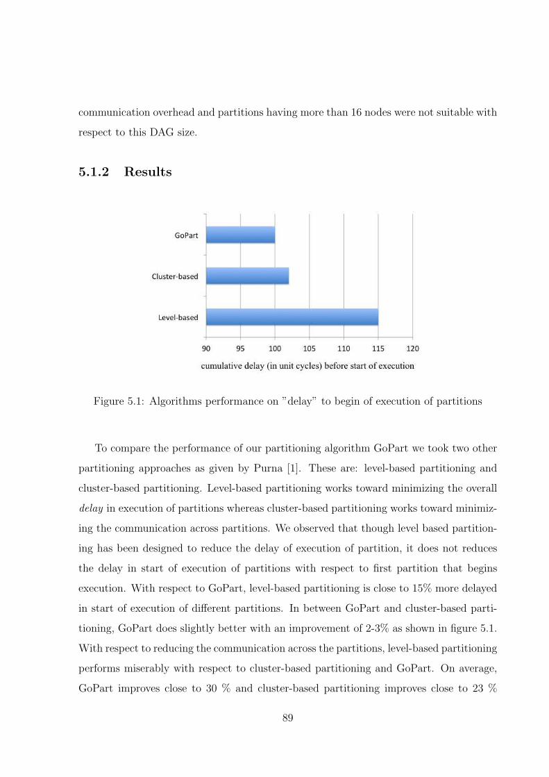
communication overhead and partitions having more than 16 nodes were not suitable with

respect to this DAG size.

5.1.2 Results

Figure 5.1: Algorithms performance on ”delay” to begin of execution of partitions

To compare the performance of our partitioning algorithm GoPart we took two other

partitioning approaches as given by Purna [1]. These are: level-based partitioning and

cluster-based partitioning. Level-based partitioning works toward minimizing the overall

delay in execution of partitions whereas cluster-based partitioning works toward minimiz-

ing the communication across partitions. We observed that though level based partition-

ing has been designed to reduce the delay of execution of partition, it does not reduces

the delay in start of execution of partitions with respect to first partition that begins

execution. With respect to GoPart, level-based partitioning is close to 15% more delayed

in start of execution of different partitions. In between GoPart and cluster-based parti-

tioning, GoPart does slightly better with an improvement of 2-3% as shown in figure 5.1.

With respect to reducing the communication across the partitions, level-based partitioning

performs miserably with respect to cluster-based partitioning and GoPart. On average,

GoPart improves close to 30 % and cluster-based partitioning improves close to 23 %

89

Figure 5.2: Algorithms performance with respect to ”communication overhead” acrossthe partitions

APPLICATIONS

Alg

orith

m p

erfo

rman

ces

over

head

(in

%)

FFT IDCT De−Block80

85

90

95

100

105

110

115

120GoPartCluster−basedLevel−based

Figure 5.3: GoPart execution performance in comparison with Cluster-based Partitioningand Level-based Partitioning

90

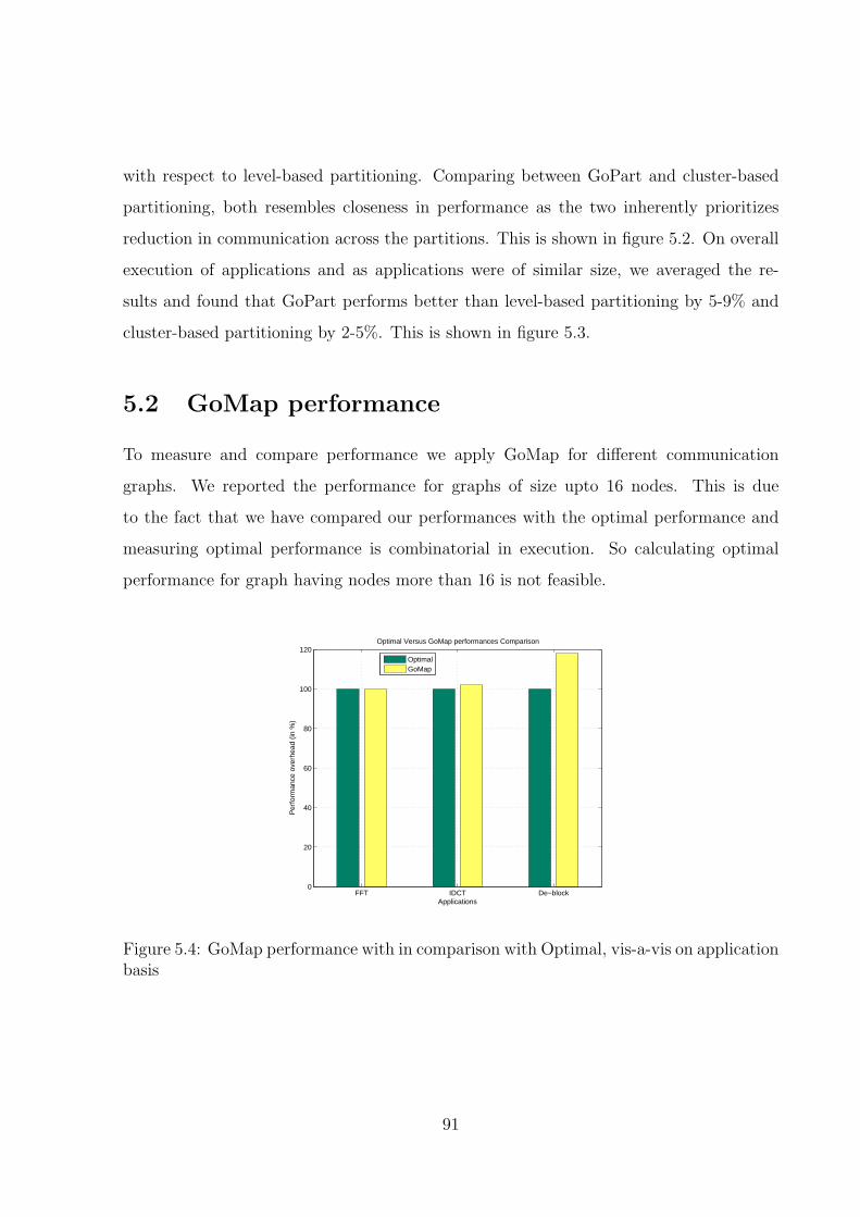
with respect to level-based partitioning. Comparing between GoPart and cluster-based

partitioning, both resembles closeness in performance as the two inherently prioritizes

reduction in communication across the partitions. This is shown in figure 5.2. On overall

execution of applications and as applications were of similar size, we averaged the re-

sults and found that GoPart performs better than level-based partitioning by 5-9% and

cluster-based partitioning by 2-5%. This is shown in figure 5.3.

5.2 GoMap performance

To measure and compare performance we apply GoMap for different communication

graphs. We reported the performance for graphs of size upto 16 nodes. This is due

to the fact that we have compared our performances with the optimal performance and

measuring optimal performance is combinatorial in execution. So calculating optimal

performance for graph having nodes more than 16 is not feasible.

FFT IDCT De−block0

20

40

60

80

100

120

Applications

Per

form

ance

ove

rhea

d (in

%)

Optimal Versus GoMap performances Comparison

OptimalGoMap

Figure 5.4: GoMap performance with in comparison with Optimal, vis-a-vis on applicationbasis

91

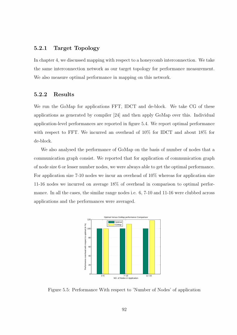
5.2.1 Target Topology

In chapter 4, we discussed mapping with respect to a honeycomb interconnection. We take

the same interconnection network as our target topology for performance measurement.

We also measure optimal performance in mapping on this network.

5.2.2 Results

We run the GoMap for applications FFT, IDCT and de-block. We take CG of these

applications as generated by compiler [24] and then apply GoMap over this. Individual

application-level performances are reported in figure 5.4. We report optimal performance

with respect to FFT. We incurred an overhead of 10% for IDCT and about 18% for

de-block.

We also analysed the performance of GoMap on the basis of number of nodes that a

communication graph consist. We reported that for application of communication graph

of node size 6 or lesser number nodes, we were always able to get the optimal performance.

For application size 7-10 nodes we incur an overhead of 10% whereas for application size

11-16 nodes we incurred on average 18% of overhead in comparison to optimal perfor-

mance. In all the cases, the similar range nodes i.e. 6, 7-10 and 11-16 were clubbed across

applications and the performances were averaged.

3−6 7−10 11−160

20

40

60

80

100

120

NO. of Nodes in Application

Per

form

ance

ove

rhea

d w

ith r

espe

ct to

opt

imal

(in

%)

Optimal Versus GoMap performance Comparison

OptimalGoMap

Figure 5.5: Performance With respect to ’Number of Nodes’ of application

92

5.3 Summary of the chapter

In this chapter we discussed and analyzed some experimental results. We presented the

results for GoPart and GoMap. We have shown that our partition algorithm GoPart

performs 2-9% better with respect to partition algorithm suggested by Purna [1]. This is

measured on an abstracted computing model for CGRA. We also discussed the necessity

and features such computing model. We showed that our mapping algorithm GoMap

performs within 18% overhead with respect to an optimal solution. This is evaluated for

communication graphs of size upto 16 nodes.

93

Chapter 6

Conclusion and Future Work

In this chapter we draw the final conclusions from the work presented in this thesis and

also discuss about some possible directions of future work.

6.1 Conclusion

In this thesis we discussed the partitioning and mapping of a computation structure. Our

focus has been efficient execution of computation structure. For partitioning, our objective

was to efficiently distribute the computation that is inherent in a computation structure

while keeping the communication across partitions minimal. For mapping, our objective

was to keep those nodes together that have more communication with each-other. We

illustrated the framework of our work in figure 6.1.

In partitioning we strongly argued for the clustering of nodes in a fashion that promotes

placing of nodes along-with their parents into same partition. We have seen that this

reduces the communication across partitions. The simple argument for this is that, total

number of communication (i.e. number of edges) in a dag is fixed, so if there is increase in

internal communication of a partition there will be same amount of decrease in external

communication (across partitions). We brought the notion of “affinity of a node” for

this. We concluded that by considering affinity of a node we reduced the communication

overhead and in-turn lesser dependency onto other partitions. We have seen that reducing

94

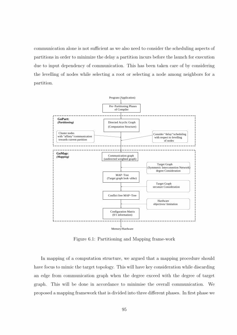
communication alone is not sufficient as we also need to consider the scheduling aspects of

partitions in order to minimize the delay a partition incurs before the launch for execution

due to input dependency of communication. This has been taken care of by considering

the levelling of nodes while selecting a root or selecting a node among neighbors for a

partition.

(Target graph look−alike)

towards current partitionwith "affinty"/communicationCluster nodes

of nodes

GoPart:

Program (Application)

Pre−Partitioning Phases

Directed Acyclic Graph

GoMap:

Target Graph (Symmetric Interconnetion Network)

Target Graph

(Mapping)

Consider "delay"/scheduling with respect to levelling

degree Consideration

strcuture Consideration

objectives/ limitationHardware

of Compiler

(Computation Structure)

MAP−Tree

Communication graph

Conflict free MAP−Tree

Configuration Matrix(0/1 information)

(undirected weighted graph)

Memory/Hardware

(Partitioning)

Figure 6.1: Partitioning and Mapping frame-work

In mapping of a computation structure, we argued that a mapping procedure should

have focus to mimic the target topology. This will have key consideration while discarding

an edge from communication graph when the degree exceed with the degree of target

graph. This will be done in accordance to minimise the overall communication. We

proposed a mapping framework that is divided into three different phases. In first phase we

95

proposed that a mapping scheme follows a methodology to convert input communication

graph to a target look-alike graph. This we termed as a MAP-Tree. Here we also brought

the notion of Cayley tree and drawn the similarity with SIN’s. In second phase we

proposed that the conflicts of this MAP-Tree are resolved by considering the structural-

constraints of target topology. First two phases give a software perspective on mapping.

Third and final phase is proposed to generate a configuration matrix which stores the

information of mapping from a hardware perspective. In next section we will discuss

that closer observation and analysis in mapping have possibility to merge second phase

into first phase. In such case, we will arrive at a conflict free MAP-Tree directly from

communication graph.

6.2 Future Work

A partitioning strategy works as per the representation of computation structure. All

previous works has been done with respect to a dag where edges and nodes do not have

operation’s and execution’s specific weights. First we want to extend the representation

of a dag by assigning weights to nodes. This is necessary because there is difference in

execution time of different mathematical, logical and bit-level operations. This enhance-

ment in computing model will give closer estimates on execution time of computation

structures. Secondly we want to have an extension into computing system which consid-

ers scheduling of partitions. This is necessary because it may be the case that PEs are

assigned to a partition only when the instruction are ready to launched for that partition

and not static bounded in advance.

For mapping, first extension we would like is to incorporate consideration of conflict

scenario at the stage of building of MAP-Tree itself. This can be done by a careful

and detailed analysis of target network. This is because at the level of unfolding the

target network we can know when a conflict will occur during construction of MAP-

Tree. Second extension we would like to study and explore mapping on other class of

interconnection networks. We have constructed mapping with respect to SINs only. Other

than SINs, there could be two categories of interconnection networks. First could be a

96

homogeneous but asymmetric networks in which degree of all nodes is same but topology

is mix of different SINs. For example a hybrid of honeycomb, 3-degree hypercube and

triangular networks. Second could be an asymmetric non-homogeneous network. For

first class of networks we can use our mapping algorithm for construction of MAP-Tree

but the resolution of conflict cases would be different. Lastly we would like to bring the

mathematical foundation in the construction of configuration matrix. This is needed (i)

to bring in exact and optimistic determination of size for configuration matrix and, (ii)

to explore the flexibility in configuration matrix.

97

Acronyms

ASIC Application Specific Integrated Circuit

GPP General Purpose Processor

CGRA Coarse Grained Reconfigurable Architecture

NoC Network on Chip

PE Processing Element

CFU Custom Function Unit

RB Resource Binder

CFG Control Flow Graph

DFG Data Flow Graph

GGGP Greedy Graph Growing Partitioning

DAG Directed Acyclic Graph

ASAP as-soon-as-possible

BFS Breadth First Search

DFS Depth First Search

SIN Symmetric Interconnection Network

TTA Transport Triggered Architecture

98

VLIW Very Large Instruction Word

AM affinity matrix

CG communication graph

RG resource graph

BB Basic-Block

LBP Level-Based Partitioning

CBP Cluster-Based Partitioning

FM Fiduccia-Mattheyses

NoC Network-on-Chip

HDL Hardware Description Language

HLL High Level Language

LAN Local Area Network

RC Reconfigurable Computing

IR Intermediate Representation

PC Program Counter

ILP Instruction Level Parallelism

ISA Instruction Set Architecture

SL Support Logic

99

Bibliography

[1] K. M. G. Purna and D. Bhatia, “Temporal partitioning and scheduling data flow graphs

for reconfigurable computers,” IEEE Trans. Computers, vol. 48, no. 6, pp. 579–590, 1999.

[2] V. Strassen, “Gaussian elimination is not optimal,” Numerische Mathe-

matik, vol. 13, pp. 354–356, 1969, 10.1007/BF02165411. [Online]. Available:

http://dx.doi.org/10.1007/BF02165411

[3] T. H. Cormen, C. E. Leiserson, R. L. Rivest, and C. Stein, Introduction to Algorithms,

2nd ed. The MIT Press, 2001.

[4] A. Aho, M. Lam, R. Sethi, and J. Ullman, Compilers: Principles, Techniques, and Tools,

2nd Edition. Addison-Wesley, 2007.

[5] S. Muchnick, High Perfomance Compilers for Parallel Computing. Addison-Wesley, 1997.

[6] R. Cytron, J. Ferrante, B. K. Rosen, M. N. Wegman, and F. K. Zadeck, “An

efficient method of computing static single assignment form,” in Proceedings of the

16th ACM SIGPLAN-SIGACT symposium on Principles of programming languages,

ser. POPL ’89. New York, NY, USA: ACM, 1989, pp. 25–35. [Online]. Available:

http://doi.acm.org/10.1145/75277.75280

[7] Chris Lattner and Vikram Adve, “LLVM: A Compilation Framework for Lifelong Program

Analysis & Transformation,” in CGO ’04: Proceedings of the international symposium on

Code generation and optimization, Washington, DC, USA, 2004.

[8] R. Cytron, J. Ferrante, B. K. Rosen, M. N. Wegman, and F. K. Zadeck, “Efficiently

computing static single assignment form and the control dependence graph,” ACM

100

Trans. Program. Lang. Syst., vol. 13, pp. 451–490, October 1991. [Online]. Available:

http://doi.acm.org/10.1145/115372.115320

[9] K. M. Kavi, B. P. Buckles, and U. N. Bhat, “A formal definition of data flow graph

models,” IEEE Trans. Comput., vol. 35, pp. 940–948, November 1986. [Online]. Available:

http://dx.doi.org/10.1109/TC.1986.1676696

[10] M. Beck, R. Johnson, and K. Pingali, “From control flow to dataflow,” Journal of Parallel

and Distributed Computing, vol. 12, no. 2, pp. 118 – 129, 1991. [Online]. Available:

http://www.sciencedirect.com/science/article/pii/0743731591900163

[11] M. Johnson, Superscalar multiprocessor design. Upper Saddle River, NJ, USA: Prentice-

Hall, Inc., 1991.

[12] H. Corporaal, “Transport Triggered Architectures. Design and Evaluation,” Ph.D. disser-

tation, January 1995.

[13] J. A. Fisher, “Very long instruction word architectures and the eli-512,” in

Proceedings of the 10th annual international symposium on Computer architecture,

ser. ISCA ’83. New York, NY, USA: ACM, 1983, pp. 140–150. [Online]. Available:

http://doi.acm.org/10.1145/800046.801649

[14] H. Corporaal, “TTAs: Missing the ILP complexity wall,” Journal of Systems

Architecture, vol. 45, no. 12-13, pp. 949 – 973, 1999. [Online]. Available:

http://www.sciencedirect.com/science/article/pii/S1383762198000460

[15] M. R. Garey and D. S. Johnson, Computers and Intractability; A Guide to the Theory of

NP-Completeness. New York, NY, USA: W. H. Freeman & Co., 1990.

[16] N. Deo, Graph Theory with Applications to Engineering and Computer Science (Prentice

Hall Series in Automatic Computation). Upper Saddle River, NJ, USA: Prentice-Hall,

Inc., 1974.

[17] A. Bondy and U. Murty, Graph theory with applications. Springer, 1976.

[18] F. T. Leighton, Introduction to parallel algorithms and architectures: array, trees, hyper-

cubes. Morgan Kaufmann Publishers Inc., 1992.

101

[19] I. Stojmenovic, “Honeycomb Networks: Topological Properties and Communication Algo-

rithms,” in IEEE ’97: Parallel Distributed Systems, vol. 8, 1997, pp. 1036–1042.

[20] B. W. Kernighan and S. Lin, “An Efficient Heuristic Procedure for Partitioning Graphs,”

The Bell system technical journal, vol. 49, no. 1, pp. 291–307, 1970.

[21] G. Karypis and V. Kumar, “Parallel multilevel series k-way partitioning scheme for irregular

graphs,” SIAM Review, vol. 41, no. 2, pp. 278–300, 1999.

[22] C. Fiduccia and R. Mattheyses, “A linear-time heuristic for improving network partitions,”

in Design Automation, 1982. 19th Conference on, june 1982, pp. 175 – 181.

[23] G. Karypis and V. Kumar, “A fast and high quality multilevel scheme for partitioning

irregular graphs,” SIAM Journal on Scientific Computing, vol. 20, no. 1, pp. 359–392,

1998.

[24] M. Alle, K. Varadarajan, A. Fell, N. Joseph, C. R. Reddy, S. Das, P. Biswas, J. Chetia, S. K.

Nandy, and R. Narayan, “REDEFINE: Runtime Reconfigurable Polymorphic ASIC,” ACM

Transactions on Embedded Systems, Special Issue on Configuring Algorithms, Processes and

Architecture, 2008.

[25] A. Robles-Kelly and E. R. Hancock, “A riemannian approach to graph embedding,”

Pattern Recogn., vol. 40, no. 3, pp. 1042–1056, Mar. 2007. [Online]. Available:

http://dx.doi.org/10.1016/j.patcog.2006.05.031

[26] J. B. Tenenbaum, V. Silva, and J. C. Langford, “A Global Geometric Framework for Non-

linear Dimensionality Reduction,” Science, vol. 290, no. 5500, pp. 2319–2323, 2000.

[27] S. T. Roweis and L. K. Saul, “Nonlinear Dimensionality Reduction by Locally Linear

Embedding,” Science, vol. 290, no. 5500, pp. 2323–2326, 2000. [Online]. Available:

http://www.sciencemag.org/cgi/content/abstract/290/5500/2323

[28] X. He, S. Yan, Y. Hu, P. Niyogi, and H. jiang Zhang, “Face recognition using laplacianfaces,”

IEEE Transactions on Pattern Analysis and Machine Intelligence, vol. 27, pp. 328–340,

2005.

[29] S. L. Scott and J. W. Baker, “Embedding the hypercube into the 3-dimension mesh.”

102

[30] E. J. Schwabe, “Embedding meshes of trees into debruijn graphs,” Inf. Process. Lett.,

vol. 43, no. 5, pp. 237–240, Oct. 1992. [Online]. Available: http://dx.doi.org/10.1016/0020-

0190(92)90217-J

[31] N. Koziris, M. Romesis, P. Tsanakas, and G. Papakonstantinou, “An efficient algorithm for

the physical mapping of clustered task graphs onto multiprocessor architectures,” in Proc.

of 8th Euromicro Workshop on Parallel and Distributed Processing, (PDP2000), IEEE.

Press, 2000, pp. 406–413.

[32] Z. Lu, L. Xia, and A. Jantsch, “Cluster-based simulated annealing for mapping cores onto

2d mesh networks on chip,” in Proceedings of the 2008 11th IEEE Workshop on Design and

Diagnostics of Electronic Circuits and Systems, 2008.

[33] S. B. Akers and B. Krishnamurthy, “A group theoretic model for symmetric interconnection

networks,” in ICPP, 1986, pp. 216–223.

[34] H. A. Bethe, “Statistical theory of superlattices,” Proceedings of the Royal Society A

Mathematical Physical and Engineering Sciences, vol. 150, no. 871, pp. 552–575, 1935.

[Online]. Available: http://rspa.royalsocietypublishing.org/cgi/doi/10.1098/rspa.1935.0122

103