Atmospheric Fronts

The material in this section is based largely on

Lectures on Dynamical Meteorologyby Roger Smith.

Atmospheric Fronts

2

Atmospheric FrontsA front is the sloping interfacial region of air between twoair masses, each of more or less uniform properties. [Frontsalso occur also in the ocean, but we will not discuss them.]

2

Atmospheric FrontsA front is the sloping interfacial region of air between twoair masses, each of more or less uniform properties. [Frontsalso occur also in the ocean, but we will not discuss them.]

The primary example is the polar front, a zone of relativelylarge horizontal temperature gradient in the mid-latitudesthat separates air masses of more uniform temperaturesthat lie polewards and equatorwards of the zone.

2

Atmospheric FrontsA front is the sloping interfacial region of air between twoair masses, each of more or less uniform properties. [Frontsalso occur also in the ocean, but we will not discuss them.]

The primary example is the polar front, a zone of relativelylarge horizontal temperature gradient in the mid-latitudesthat separates air masses of more uniform temperaturesthat lie polewards and equatorwards of the zone.

This is associated with the midlatitude westerlies, havingtheir maximum at the jetstream in the upper troposphere.This is the Polar Front Jet.

2

Atmospheric FrontsA front is the sloping interfacial region of air between twoair masses, each of more or less uniform properties. [Frontsalso occur also in the ocean, but we will not discuss them.]

The primary example is the polar front, a zone of relativelylarge horizontal temperature gradient in the mid-latitudesthat separates air masses of more uniform temperaturesthat lie polewards and equatorwards of the zone.

This is associated with the midlatitude westerlies, havingtheir maximum at the jetstream in the upper troposphere.This is the Polar Front Jet.

Regionally, where the polar front is particularly pronounced,we have cold and warm fronts associated with extra-tropicalcyclones.

2

Atmospheric FrontsA front is the sloping interfacial region of air between twoair masses, each of more or less uniform properties. [Frontsalso occur also in the ocean, but we will not discuss them.]

The primary example is the polar front, a zone of relativelylarge horizontal temperature gradient in the mid-latitudesthat separates air masses of more uniform temperaturesthat lie polewards and equatorwards of the zone.

This is associated with the midlatitude westerlies, havingtheir maximum at the jetstream in the upper troposphere.This is the Polar Front Jet.

Regionally, where the polar front is particularly pronounced,we have cold and warm fronts associated with extra-tropicalcyclones.

Sharp temperature differences can occur across a frontalsurface: several degrees over a few kilometres.

2

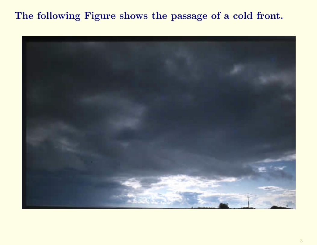
The following Figure shows the passage of a cold front.

3

Composite meridional cross-section at 80◦W of mean temperature and

the zonal component of geostrophic wind computed from 12 individual

cross-sections. The means were computed with respect to the position

of the polar front in individual cases (from Palmen and Newton, 1948).

4

Analysed surface pressure, storm in October, 2000.5

Margules’ Model

6

Margules’ Model

Max Margules (1856–1920)

The simplest model repre-senting a frontal discontinu-ity is Margules’ model.

In this model, the front is ide-alized as a sharp, plane, tem-perature discontinuity sepa-rating two inviscid, homoge-neous, geostrophic flows.

6

Configuration of Margules’ frontal model.Subscripts 1 and 2 refer to the warm and cold air masses.

7

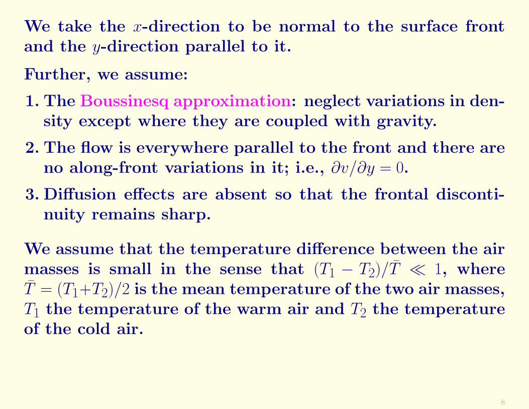
We take the x-direction to be normal to the surface frontand the y-direction parallel to it.

8

We take the x-direction to be normal to the surface frontand the y-direction parallel to it.

Further, we assume:

1. The Boussinesq approximation: neglect variations in den-sity except where they are coupled with gravity.

8

We take the x-direction to be normal to the surface frontand the y-direction parallel to it.

Further, we assume:

1. The Boussinesq approximation: neglect variations in den-sity except where they are coupled with gravity.

2. The flow is everywhere parallel to the front and there areno along-front variations in it; i.e., ∂v/∂y = 0.

8

We take the x-direction to be normal to the surface frontand the y-direction parallel to it.

Further, we assume:

1. The Boussinesq approximation: neglect variations in den-sity except where they are coupled with gravity.

2. The flow is everywhere parallel to the front and there areno along-front variations in it; i.e., ∂v/∂y = 0.

3. Diffusion effects are absent so that the frontal disconti-nuity remains sharp.

8

We take the x-direction to be normal to the surface frontand the y-direction parallel to it.

Further, we assume:

1. The Boussinesq approximation: neglect variations in den-sity except where they are coupled with gravity.

2. The flow is everywhere parallel to the front and there areno along-front variations in it; i.e., ∂v/∂y = 0.

3. Diffusion effects are absent so that the frontal disconti-nuity remains sharp.

We assume that the temperature difference between the airmasses is small in the sense that (T1 − T2)/T � 1, whereT = (T1+T2)/2 is the mean temperature of the two air masses,T1 the temperature of the warm air and T2 the temperatureof the cold air.

8

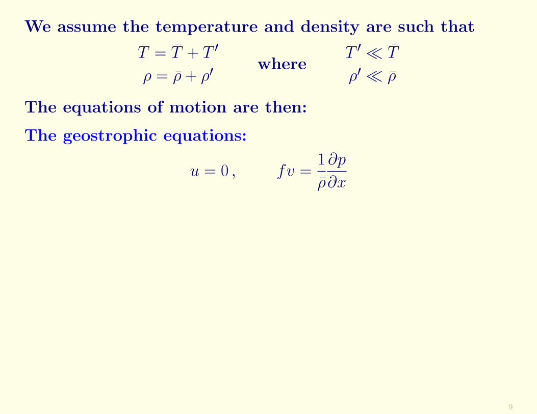
We assume the temperature and density are such that

T = T + T ′

ρ = ρ + ρ′where

T ′ � T

ρ′ � ρ

9

We assume the temperature and density are such that

T = T + T ′

ρ = ρ + ρ′where

T ′ � T

ρ′ � ρ

The equations of motion are then:

The geostrophic equations:

u = 0 , fv =1

ρ

∂p

∂x

9

We assume the temperature and density are such that

T = T + T ′

ρ = ρ + ρ′where

T ′ � T

ρ′ � ρ

The equations of motion are then:

The geostrophic equations:

u = 0 , fv =1

ρ

∂p

∂x

The hydrostatic equation:

1

ρ

∂p

∂z= −g(T − T ′)

T

9

We assume the temperature and density are such that

T = T + T ′

ρ = ρ + ρ′where

T ′ � T

ρ′ � ρ

The equations of motion are then:

The geostrophic equations:

u = 0 , fv =1

ρ

∂p

∂x

The hydrostatic equation:

1

ρ

∂p

∂z= −g(T − T ′)

T

The continuity equation:

∂u

∂x+

∂w

∂z= 0

9

In general, the temperature decreases with height in theatmosphere.

10

In general, the temperature decreases with height in theatmosphere.

In Margules’ model the vertical temperature gradient ineach air mass is assumed to be zero.

10

In general, the temperature decreases with height in theatmosphere.

In Margules’ model the vertical temperature gradient ineach air mass is assumed to be zero.

In fact, the temperature in each airmass is constant, varyingneither in the horizontal nor in the vertical direction.

10

In general, the temperature decreases with height in theatmosphere.

In Margules’ model the vertical temperature gradient ineach air mass is assumed to be zero.

In fact, the temperature in each airmass is constant, varyingneither in the horizontal nor in the vertical direction.

We consider this to be the limiting case of the situationin which the temperature gradients are very small exceptacross the frontal zone, where they are very large.

10

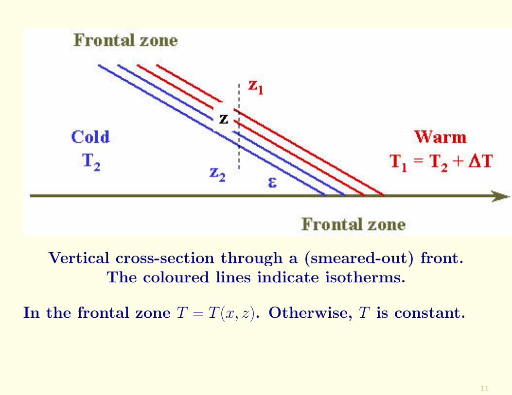
Vertical cross-section through a (smeared-out) front.The coloured lines indicate isotherms.

In the frontal zone T = T (x, z). Otherwise, T is constant.

11

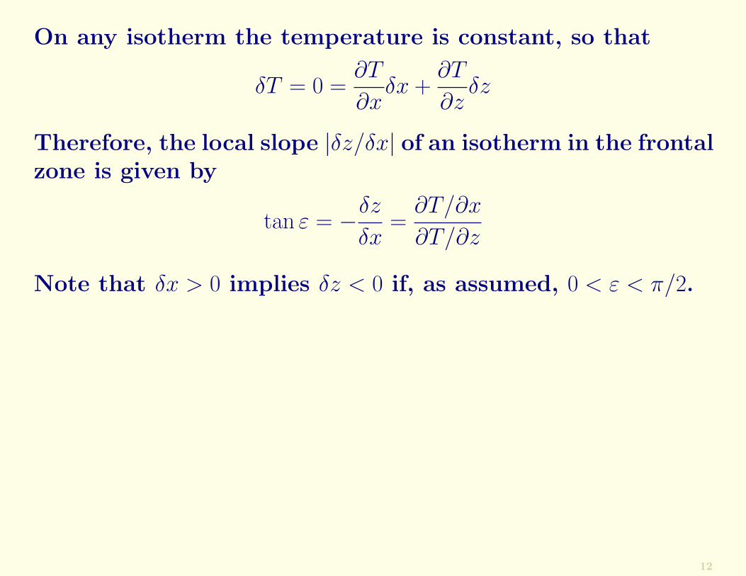
On any isotherm the temperature is constant, so that

δT = 0 =∂T

∂xδx +

∂T

∂zδz

12

On any isotherm the temperature is constant, so that

δT = 0 =∂T

∂xδx +

∂T

∂zδz

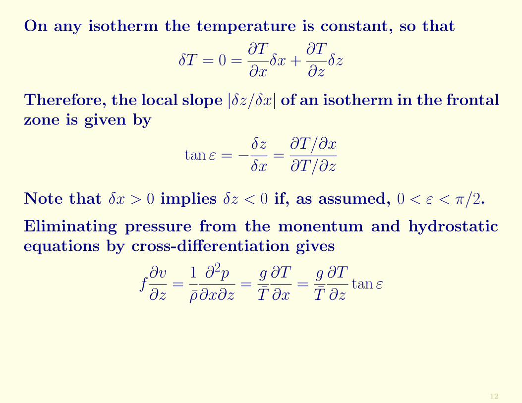
Therefore, the local slope |δz/δx| of an isotherm in the frontalzone is given by

tan ε = −δz

δx=

∂T/∂x

∂T/∂z

12

On any isotherm the temperature is constant, so that

δT = 0 =∂T

∂xδx +

∂T

∂zδz

Therefore, the local slope |δz/δx| of an isotherm in the frontalzone is given by

tan ε = −δz

δx=

∂T/∂x

∂T/∂z

Note that δx > 0 implies δz < 0 if, as assumed, 0 < ε < π/2.

12

On any isotherm the temperature is constant, so that

δT = 0 =∂T

∂xδx +

∂T

∂zδz

Therefore, the local slope |δz/δx| of an isotherm in the frontalzone is given by

tan ε = −δz

δx=

∂T/∂x

∂T/∂z

Note that δx > 0 implies δz < 0 if, as assumed, 0 < ε < π/2.

Eliminating pressure from the monentum and hydrostaticequations by cross-differentiation gives

f∂v

∂z=

1

ρ

∂2p

∂x∂z=

g

T

∂T

∂x=

g

T

∂T

∂ztan ε

12

On any isotherm the temperature is constant, so that

δT = 0 =∂T

∂xδx +

∂T

∂zδz

Therefore, the local slope |δz/δx| of an isotherm in the frontalzone is given by

tan ε = −δz

δx=

∂T/∂x

∂T/∂z

Note that δx > 0 implies δz < 0 if, as assumed, 0 < ε < π/2.

Eliminating pressure from the monentum and hydrostaticequations by cross-differentiation gives

f∂v

∂z=

1

ρ

∂2p

∂x∂z=

g

T

∂T

∂x=

g

T

∂T

∂ztan ε

This is simply the thermal wind equation relating the ver-tical shear across the front to the horizontal temperaturecontrast across it.

12

Repeat:

f∂v

∂z=

g

T

∂T

∂ztan ε

13

Repeat:

f∂v

∂z=

g

T

∂T

∂ztan ε

Solving for the slope, we get

tan ε =fT ∂v/∂z

g∂T/∂z

13

Repeat:

f∂v

∂z=

g

T

∂T

∂ztan ε

Solving for the slope, we get

tan ε =fT ∂v/∂z

g∂T/∂z

Integrating across the frontal zone, we get

tan ε =fT

g

δv

δTwhere δv and δT are the changes in along-front wind andtemperature across the front.

13

Repeat:

f∂v

∂z=

g

T

∂T

∂ztan ε

Solving for the slope, we get

tan ε =fT ∂v/∂z

g∂T/∂z

Integrating across the frontal zone, we get

tan ε =fT

g

δv

δTwhere δv and δT are the changes in along-front wind andtemperature across the front.

This is Margules’ formula and relates the slope of the frontalsurface to the change in geostrophic wind speed across it andto the temperature difference across it.

13

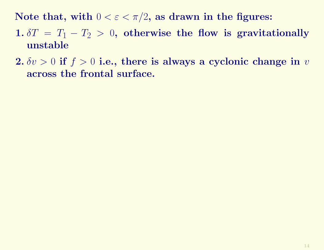
Note that, with 0 < ε < π/2, as drawn in the figures:

1. δT = T1 − T2 > 0, otherwise the flow is gravitationallyunstable

14

Note that, with 0 < ε < π/2, as drawn in the figures:

1. δT = T1 − T2 > 0, otherwise the flow is gravitationallyunstable

2. δv > 0 if f > 0 i.e., there is always a cyclonic change in vacross the frontal surface.

14

Note that, with 0 < ε < π/2, as drawn in the figures:

1. δT = T1 − T2 > 0, otherwise the flow is gravitationallyunstable

2. δv > 0 if f > 0 i.e., there is always a cyclonic change in vacross the frontal surface.

Note, however, that it is not necessary that v1 > 0 and v2 < 0separately; only the change in v is important.

14

Note that, with 0 < ε < π/2, as drawn in the figures:

1. δT = T1 − T2 > 0, otherwise the flow is gravitationallyunstable

2. δv > 0 if f > 0 i.e., there is always a cyclonic change in vacross the frontal surface.

Note, however, that it is not necessary that v1 > 0 and v2 < 0separately; only the change in v is important.

There are three possible configurations as illustrated below.

14

Surface isobars in Margules’ stationary front model hemisphereshowing the three possible cases with the cold air to the left:

(left) v1 > 0, v2 < 0; (centre) 0 < v2 < v1; (right) v2 < v1 < 0;

The surface pressure variation along the line AB is also shown.15

Margules’ solution is an exact solution of the Euler equa-tions of motion in a rotating frame, as the nonlinear andtime dependent terms vanish identically.

16

Margules’ solution is an exact solution of the Euler equa-tions of motion in a rotating frame, as the nonlinear andtime dependent terms vanish identically.

Margules’ formula is a diagnostic one for a stationary, orquasi-stationary front; it tells us nothing about the forma-tion (frontogenesis) or decay (frontolysis) of fronts.

16

Margules’ solution is an exact solution of the Euler equa-tions of motion in a rotating frame, as the nonlinear andtime dependent terms vanish identically.

Margules’ formula is a diagnostic one for a stationary, orquasi-stationary front; it tells us nothing about the forma-tion (frontogenesis) or decay (frontolysis) of fronts.

It is of little practical use in forecasting, since active fronts,which are responsible for a good deal of the ‘significantweather’ in middle latitudes, are much more dynamic.

16

Margules’ solution is an exact solution of the Euler equa-tions of motion in a rotating frame, as the nonlinear andtime dependent terms vanish identically.

Margules’ formula is a diagnostic one for a stationary, orquasi-stationary front; it tells us nothing about the forma-tion (frontogenesis) or decay (frontolysis) of fronts.

It is of little practical use in forecasting, since active fronts,which are responsible for a good deal of the ‘significantweather’ in middle latitudes, are much more dynamic.

Real fronts are always associated with rising vertical mo-tion and are normally accompanied by precipitation.

16

Margules’ solution is an exact solution of the Euler equa-tions of motion in a rotating frame, as the nonlinear andtime dependent terms vanish identically.

Margules’ formula is a diagnostic one for a stationary, orquasi-stationary front; it tells us nothing about the forma-tion (frontogenesis) or decay (frontolysis) of fronts.

It is of little practical use in forecasting, since active fronts,which are responsible for a good deal of the ‘significantweather’ in middle latitudes, are much more dynamic.

Real fronts are always associated with rising vertical mo-tion and are normally accompanied by precipitation.

Moreover, real cold and warm fronts are generally not sta-tionary, but may have speeds comparable to the horizontalwind itself. We illustrate fronts in motion in the followingfigure.

16

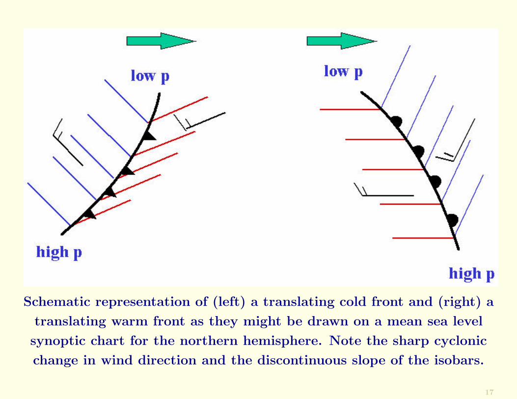
Schematic representation of (left) a translating cold front and (right) a

translating warm front as they might be drawn on a mean sea level

synoptic chart for the northern hemisphere. Note the sharp cyclonic

change in wind direction and the discontinuous slope of the isobars.

17

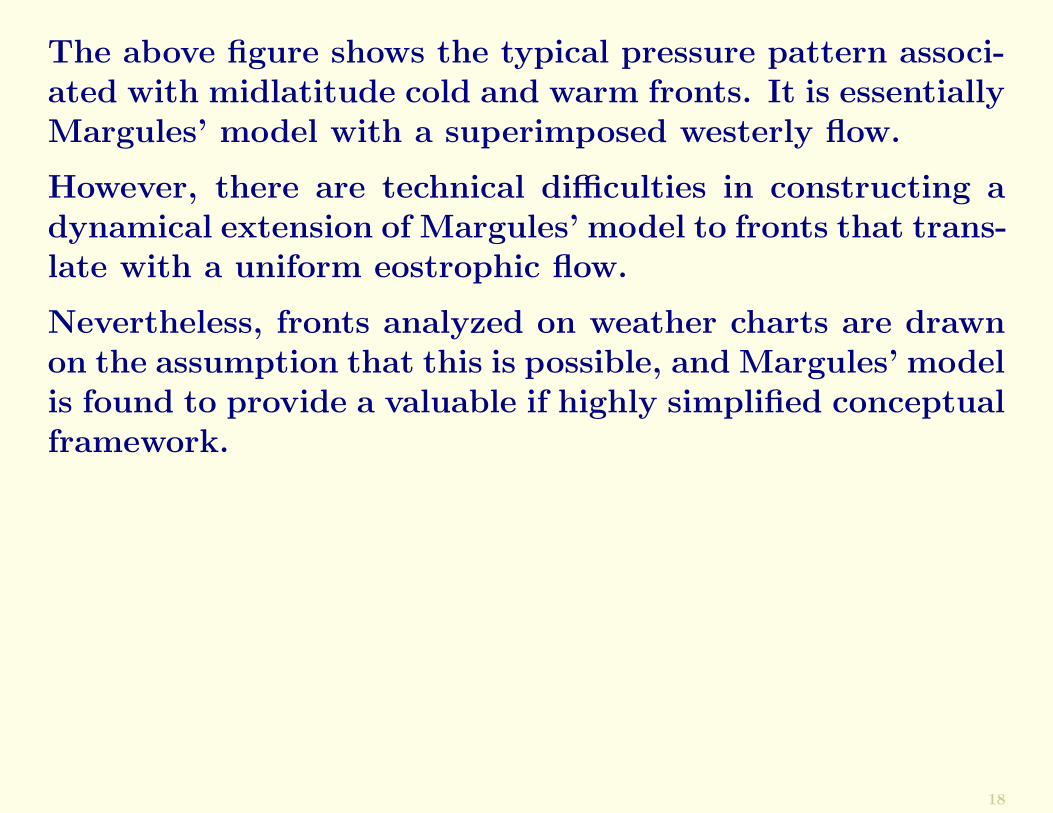
The above figure shows the typical pressure pattern associ-ated with midlatitude cold and warm fronts. It is essentiallyMargules’ model with a superimposed westerly flow.

18

The above figure shows the typical pressure pattern associ-ated with midlatitude cold and warm fronts. It is essentiallyMargules’ model with a superimposed westerly flow.

However, there are technical difficulties in constructing adynamical extension of Margules’ model to fronts that trans-late with a uniform eostrophic flow.

18

The above figure shows the typical pressure pattern associ-ated with midlatitude cold and warm fronts. It is essentiallyMargules’ model with a superimposed westerly flow.

However, there are technical difficulties in constructing adynamical extension of Margules’ model to fronts that trans-late with a uniform eostrophic flow.

Nevertheless, fronts analyzed on weather charts are drawnon the assumption that this is possible, and Margules’ modelis found to provide a valuable if highly simplified conceptualframework.

18

The above figure shows the typical pressure pattern associ-ated with midlatitude cold and warm fronts. It is essentiallyMargules’ model with a superimposed westerly flow.

However, there are technical difficulties in constructing adynamical extension of Margules’ model to fronts that trans-late with a uniform eostrophic flow.

Nevertheless, fronts analyzed on weather charts are drawnon the assumption that this is possible, and Margules’ modelis found to provide a valuable if highly simplified conceptualframework.

It is interesting that Margules developed his model of an at-mospheric discontinuity some fifteen years before the emer-gence of the frontal models of the Norwegian School. Therewere other precursors of frontal theory in Germany and inBritain.

18

Exercise: Check the dimensional consistency of Margules’Formula.

Calculate the frontal slope using Margules’ Formula, assum-ing that the mean temperature is T = 280K, the Coriolisparameter f = 10−4 s−1, g = 10ms−2, the difference in wind-speed across the front is δv = 12ms−1 and the difference intemperature is δt = 4K.

19

Exercise: Check the dimensional consistency of Margules’Formula.

Calculate the frontal slope using Margules’ Formula, assum-ing that the mean temperature is T = 280K, the Coriolisparameter f = 10−4 s−1, g = 10ms−2, the difference in wind-speed across the front is δv = 12ms−1 and the difference intemperature is δt = 4K.

Solution: . . .Answer: ε ≈ 1/120.

19