patrick seamus haughian
TRANSCRIPT
PhD-FSTC-2018-65
The Faculty of Sciences, Technology and Communication
DISSERTATION
Defence held on 18/10/2018 in Luxembourg
to obtain the degree of
DOCTEUR DE L’UNIVERSITÉ DU LUXEMBOURG
EN PHYSIQUE
by
Patrick Seamus HAUGHIAN Born on 4 February 1992 in Troisdorf (Germany)
TRANSPORT AND THERMODYNAMICS
IN DRIVEN QUANTUM SYSTEMS
Dissertation defence committee
Dr Thomas Schmidt, dissertation supervisor Associate Professor, Université du Luxembourg
Dr Christoph Bruder, Vice Chairman Professor, Universität Basel
Dr Andreas Michels, Chairman Associate Professor, Université du Luxembourg
Dr Andreas Nunnenkamp Royal Society Research Fellow, University of Cambridge
Dr Massimiliano Esposito Professor, Université du Luxembourg

Abstract
This thesis studies the nonequilibrium properties of quantum dots with regardto electrical conduction as well as thermodynamics. The work documented hereshows how these properties behave under the influence of time-dependent driveprotocols, pursuing two main lines of inquiry. The first concerns the interplay be-tween nanomechanics and drive: In nanomechanical systems with strong couplingbetween the charge and vibrational sectors, conductance is strongly suppressed, aneffect known as Franck-Condon blockade. Using a model Hamiltonian for a molec-ular quantum dot coupled to a pair of leads, it is shown here that this blockade canbe exponentially lifted by resonantly driving the dot. Moreover, a multi-drive pro-tocol is proposed for such a system to facilitate charge pumping that enjoys thesame exponential amplification. The second line of inquiry moves beyond chargetransport, examining the thermodynamics of a driven quantum dot coupled to alead. Taking a Green’s function approach, it is found that the laws of thermody-namics can be formulated for arbitrary dot-lead coupling strength in the presenceof dot and coupling drive, as long as the drive protocol only exhibits mild non-adiabaticity. Finally, the effects of initial states are studied in this situation, provingthat the integrated work production in the long-time limit conforms to the secondlaw of thermodynamics for a wide class of initial states and arbitrary drive andcoupling strength.
Contents
Introduction 3
1 Background and methods 61.1 Molecular quantum dots . . . . . . . . . . . . . . . . . . . . . . 61.2 Non-equilibrium Green’s functions . . . . . . . . . . . . . . . . . 10
1.2.1 Keldysh technique . . . . . . . . . . . . . . . . . . . . . 101.2.2 Occupation of a single level coupled to a lead . . . . . . . 131.2.3 From Keldysh to current . . . . . . . . . . . . . . . . . . 21
1.3 Floquet expansion for driven systems . . . . . . . . . . . . . . . . 251.4 Open quantum systems and master equations . . . . . . . . . . . 27
1.4.1 From von Neumann to Lindblad . . . . . . . . . . . . . . 271.4.2 A note on Markovianity . . . . . . . . . . . . . . . . . . 29
1.5 Quantum thermodynamics: An overview . . . . . . . . . . . . . . 321.5.1 Open quantum systems and weak-coupling thermodynamics 331.5.2 Stochastic thermodynamics . . . . . . . . . . . . . . . . 341.5.3 Hamiltonians of mean force . . . . . . . . . . . . . . . . 36
2 Results 382.1 Lifting the Franck-Condon blockade
in carbon nanotube quantum dots . . . . . . . . . . . . . . . . . . 382.1.1 Introduction . . . . . . . . . . . . . . . . . . . . . . . . . 382.1.2 Model . . . . . . . . . . . . . . . . . . . . . . . . . . . . 402.1.3 Polaron tunneling approximation . . . . . . . . . . . . . . 432.1.4 Born-Markov analysis . . . . . . . . . . . . . . . . . . . 492.1.5 Conclusion . . . . . . . . . . . . . . . . . . . . . . . . . 552.1.6 Appendix: Details on the NEGF approach . . . . . . . . . 572.1.7 Appendix: Tunneling rates for Fock vibron state . . . . . 60
2.2 Charge pumping in strongly coupled molecular quantum dots . . . 622.2.1 Introduction . . . . . . . . . . . . . . . . . . . . . . . . . 622.2.2 Model . . . . . . . . . . . . . . . . . . . . . . . . . . . . 632.2.3 Floquet Green’s functions . . . . . . . . . . . . . . . . . 652.2.4 Current under bias . . . . . . . . . . . . . . . . . . . . . 682.2.5 Polaron pumping . . . . . . . . . . . . . . . . . . . . . . 69
1
2.2.6 Conclusion . . . . . . . . . . . . . . . . . . . . . . . . . 732.2.7 Appendix: Bare Green’s functions . . . . . . . . . . . . . 742.2.8 Appendix: Self-energy . . . . . . . . . . . . . . . . . . . 76
2.3 Quantum thermodynamics of the resonant-level modelwith driven system-bath coupling . . . . . . . . . . . . . . . . . . 772.3.1 Introduction . . . . . . . . . . . . . . . . . . . . . . . . . 772.3.2 Resonant-level model . . . . . . . . . . . . . . . . . . . . 792.3.3 Thermodynamic definitions and first law . . . . . . . . . 822.3.4 Link to equilibrium . . . . . . . . . . . . . . . . . . . . . 832.3.5 Second law . . . . . . . . . . . . . . . . . . . . . . . . . 852.3.6 Comparison with exact numerical results . . . . . . . . . 872.3.7 Conclusions . . . . . . . . . . . . . . . . . . . . . . . . . 882.3.8 Appendix: Adiabatic limit . . . . . . . . . . . . . . . . . 902.3.9 Appendix: Quasi-adiabatic expansion . . . . . . . . . . . 91
2.4 Initial states in quantum thermodynamics . . . . . . . . . . . . . 932.4.1 Introduction . . . . . . . . . . . . . . . . . . . . . . . . . 932.4.2 Model . . . . . . . . . . . . . . . . . . . . . . . . . . . . 942.4.3 Work production . . . . . . . . . . . . . . . . . . . . . . 962.4.4 Long-time limit . . . . . . . . . . . . . . . . . . . . . . . 982.4.5 Conclusion . . . . . . . . . . . . . . . . . . . . . . . . . 992.4.6 Appendix: Expectation values . . . . . . . . . . . . . . . 100
3 Summary 104
Bibliography 107
Acknowledgments 121
List of publications 122
2
Introduction
In one way or another, transport physics serves as the foundation for much ofmodern civilization. Technical processes and machines that depend on preciseengineering of electrical, heat and matter currents are innumerable, and the ever-increasing sophistication of tomorrow’s technology relies upon today’s research.Among the many aspects of the theory of transport, the ones under investigation inthis thesis are those connected with the quantum regime and thermodynamics.
Quantum mechanics is the blockbuster discovery of 20th century physics: Ithas revolutionized our understanding of the microscopic world, and its implica-tions reach far beyond academic studies, into everyday life. What started out asan attempt by Planck to understand black-body radiation [1] has since evolved intoa comprehensive theory, leading to a torrent of inventions such as the laser, thetransistor, and modern medical imaging, just to name three. The sub-field of con-densed matter physics, which has as its subject the study of interacting quantummany-particle systems, has proven to be particularly fruitful in terms of applica-tions to engineering and materials science. In the evolution of modern condensedmatter physics, two convergent directions have been apparent: On the one hand,with increasing development of the theory and powerful computational tools, ourconceptual understanding of quantum systems has grown to include ever morecomplex and large many-particle systems. On the other hand, the evolution ofour experimental capabilities have afforded us more and more precise control overever smaller objects, even down to single-atom devices [2]. These developmentshave converged to form the burgeoning field of nanoscale physics, where quan-tum theory, simulation, and experiments are used in concert to build the devicesof the future. Some of these devices have already reshaped the technology of thepresent: Decades of miniaturization efforts have placed the current state of tran-sistor development firmly into the nanoscale, and modern solar cells and LEDswould be unthinkable without knowledge of nanoscale physics. The nanoscale ishome to a remarkable wealth of phenomenology, including electronics as well asoptical and mechanical effects, all of which may interact in ways too numerous tolist. Equipped with such a large toolkit, the research directions available to today’snanoscientists are as boundless as the possible technologies that may grow fromtheir work.
The beginnings of thermodynamics lie further in the past [3] than those ofquantum mechanics. Developed in the 19th century as a framework for the under-
3

standing of heat, work, temperature and energy, thermodynamics is invaluable inthe design of machines and work cycles and provided the scientific underpinningof the industrial revolution. Its laws were first formulated in a phenomenologicalmanner, without reference to any microscopic theory. Even though it was later un-derstood to arise from statistical mechanics in the limit of large particle number,this limit lies on the scale of Avogadro’s constant NA ≈ 6 × 10²³, and thereforeclassical thermodynamics cannot be expected to hold at all scales. Nonetheless,thermodynamics and its laws have long since become a mainstay not only in engi-neering and physics, but also in computer science, where the theory of informationmakes extensive use of entropy and related concepts [4, 5, 6].
Fluxes and currents are natural objects in thermodynamics. Therefore, the con-nections between transport theory and thermodynamics, such as the effect of cur-rent flowing as a result of temperature gradients [7], have been explored early on.The path between thermodynamics and quantum mechanics is far less traveled:Since the former has its classical applications in macroscopic systems, and the do-main of the latter are chiefly microscopic systems, a vast difference in scale haskept the two theories relatively separated, with only occasional historical overlap,such as the early proposal for a quantum engine [8] and the analysis of thermody-namics in a certain class of open systems [9].
In recent decades, the advent of nanoscale physics has led to a change in per-spective: The range of device sizes accessible in experiments has been extendeddown to a regime where quantum effects are paramount. These devices hold greatpromise in many regards, such as the miniaturization of electronic components,the design of innovative measurement schemes and quantum machines, as well asin the context of quantum computation. Heat production has emerged as a seri-ous bottleneck for the performance of these systems, and so a consistent theory ofquantum thermodynamics has become extremely desirable. Such a theory wouldneed to re-formulate the laws of thermodynamics for quantum systems while asmuch as possible of the generality of their classical counterpart. Moreover, due tothe prominence of non-stationary effects at the nanoscale, quantum thermodynam-ics needs to remain valid far from the equilibrium or adiabatic settings commonin macroscopic settings. Considerable progress has already been achieved in thisendeavor, both in terms of conceptual foundations, and regarding the behavior ofcertain model systems, but an overarching framework is still lacking.
The work documented in this thesis is performed on the frontier of nanoscalephysics, at the confluence of fields of transport theory, quantum mechanics, andthermodynamics. The presentation is structured as two parts: First, Ch. 1 is used tolay out the methods and provide context for the research to be viewed in. Second,the results are laid out in Ch. 2. The beginning of the expository chapter gives ashort historical overview of the relevant nanodevices in Sec. 1.1. There, the focuslies on quantum dots, meso- or nanoscale structures that combine the quantizedenergy structure of quantum systems with the ability to be integrated into electricalcircuits. Systems of this kind provide a versatile platform for device developmentand are studied under various aspects in the remainder of this work. Next, the meth-
4
ods used to this end are laid out in Secs. 1.2 to 1.4. The exposition concludes inSec. 1.5 with a sketch of the current state of quantum thermodynamics and the chal-lenges that still need to be addressed. The first two sections of the results concernthemselves with using time-dependent driving potentials to manipulate the electrictransport through a strongly coupled nanomechanical quantum dot: In Sec. 2.1 itis shown that by driving the quantum dot resonantly with its vibrational mode, itsconductance can be increased exponentially, thus lifting the transport blockade in-herent in strongly coupled electromechanical systems. Then, in Sec. 2.2, a morecomplex drive protocol is proposed to pump charge in either direction across such ananomechanical quantum dot. It is shown that the current pumped in this way alsoenjoys the exponential amplification discovered in the previous section. The thirdand fourth result sections are devoted to quantum thermodynamics: Sec. 2.3 showshow to use nonequilibrium Green’s functions to establish the laws of thermody-namics in a model of a quantum dot coupled with arbitrary strength to a metalliclead, subject to a multi-drive protocol. Lastly, Sec. 2.4 adds the initial state of thesetup to the consideration, and links the quantum thermodynamics of such a modelsystem with the general framework of stochastic thermodynamics. This connec-tion is used to show that the work produced under a general drive protocol behavesaccording to the second law of thermodynamics for a wide class of initial states,as long as the long-time limit is considered. Finally, a summary discussion is pro-vided in Ch. 3, reviewing the documented findings and pointing out directions forfuture research.
5
Chapter 1
Background and methods
1.1 Molecular quantum dots
Quantum dots are mesoscopic structures with individually spaced energy levels.A plethora of different implementations of such systems have emerged over thepast decades, with applications ranging from display technology [10] over medicalimaging [11] to proposals for quantum computation [12].
This thesis concerns itself with the transport properties of quantum dots. Sinceour results build upon many years’ worth of insight obtained previously, this chap-ter will be used to give an outline of this body of knowledge.
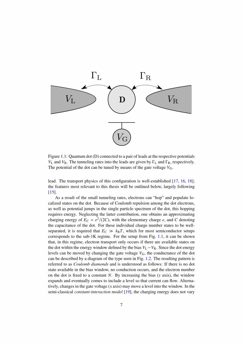
The physics of quantum dots has its beginning in the study of semiconductornanocrystals [13, 14], where individual quantum states can be examined even insystems consisting of several thousand atoms. Their properties are evocative ofzero-dimensional quantum systems, hence the name quantum dot. The optical andelectronic features of quantum dots were soon realized and spurred a flurry of re-search. This led to the development of various platforms to realize quantum dots,as well as various ways of embedding them into electrical circuits, thus bringinginto focus their conductive properties [15]. In order to probe the conductance of aquantum dot, it is connected to a number of leads, across which voltages can be ap-plied. A schematic representation of such a setup is given in Fig. 1.1. The physicsthat manifests in such a setup strongly depends on its parameters and energy scales[16]. These include the lead temperature T , the applied potentials Vα, the tunnel-ing rates Γα between the dot and the leads, as well as the internal properties ofthe lead, such as its quantum level spacing ∆ and the strength of the interaction be-tween electrons on the dot. Signatures of the quantization of the energies on the dotcan only be observed if these energies are spaced sufficiently far apart, in particu-lar further than typical thermal fluctuations in energy. This dictates the condition∆ > kBT , where kB denotes the Boltzmann constant. Moreover, the level spacing ∆
needs to be compared to the tunneling rates Γα. The case ∆ Γα is known as weakcoupling. In this case, the energy levels on the dot still exhibit clear peak signa-tures, with a width on the scale of Γ acquired by hybridization to the energies in the
6
D
Figure 1.1: Quantum dot (D) connected to a pair of leads at the respective potentialsVL and VR. The tunneling rates into the leads are given by ΓL and ΓR, respectively.The potential of the dot can be tuned by means of the gate voltage VG.
lead. The transport physics of this configuration is well-established [17, 16, 18];the features most relevant to this thesis will be outlined below, largely following[15].
As a result of the small tunneling rates, electrons can “hop” and populate lo-calized states on the dot. Because of Coulomb repulsion among the dot electrons,as well as potential jumps in the single particle spectrum of the dot, this hoppingrequires energy. Neglecting the latter contribution, one obtains an approximatingcharging energy of EC = e2/(2C), with the elementary charge e, and C denotingthe capacitance of the dot. For these individual charge number states to be well-separated, it is required that EC kBT , which for most semiconductor setupscorresponds to the sub-1K regime. For the setup from Fig. 1.1, it can be shownthat, in this regime, electron transport only occurs if there are available states onthe dot within the energy window defined by the bias VL−VR. Since the dot energylevels can be moved by changing the gate voltage VG, the conductance of the dotcan be described by a diagram of the type seen in Fig. 1.2. The resulting pattern isreferred to as Coulomb diamonds and is understood as follows: If there is no dotstate available in the bias window, no conduction occurs, and the electron numberon the dot is fixed to a constant N. By increasing the bias (y axis), the windowexpands and eventually comes to include a level so that current can flow. Alterna-tively, changes in the gate voltage (x axis) may move a level into the window. In thesemi-classical constant-interaction model [19], the charging energy does not vary
7
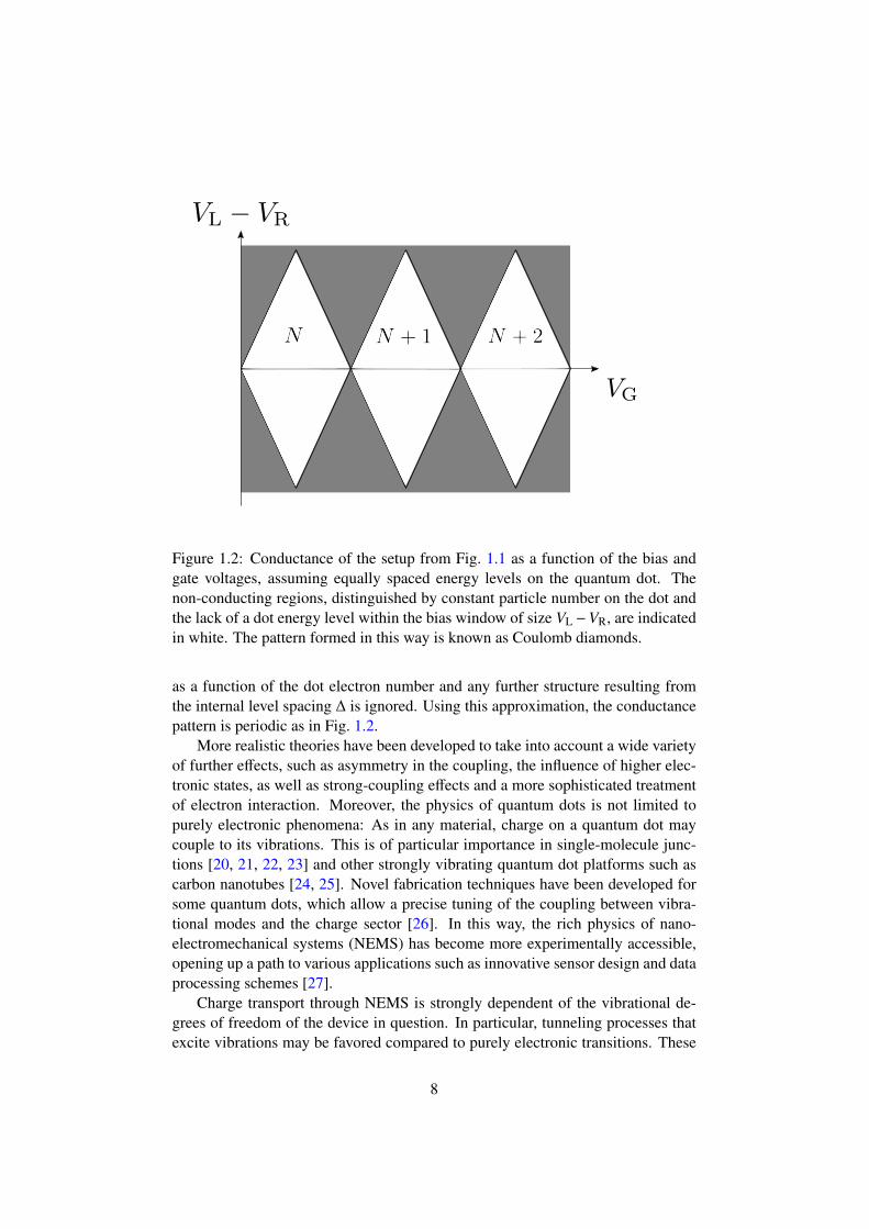
Figure 1.2: Conductance of the setup from Fig. 1.1 as a function of the bias andgate voltages, assuming equally spaced energy levels on the quantum dot. Thenon-conducting regions, distinguished by constant particle number on the dot andthe lack of a dot energy level within the bias window of size VL −VR, are indicatedin white. The pattern formed in this way is known as Coulomb diamonds.
as a function of the dot electron number and any further structure resulting fromthe internal level spacing ∆ is ignored. Using this approximation, the conductancepattern is periodic as in Fig. 1.2.
More realistic theories have been developed to take into account a wide varietyof further effects, such as asymmetry in the coupling, the influence of higher elec-tronic states, as well as strong-coupling effects and a more sophisticated treatmentof electron interaction. Moreover, the physics of quantum dots is not limited topurely electronic phenomena: As in any material, charge on a quantum dot maycouple to its vibrations. This is of particular importance in single-molecule junc-tions [20, 21, 22, 23] and other strongly vibrating quantum dot platforms such ascarbon nanotubes [24, 25]. Novel fabrication techniques have been developed forsome quantum dots, which allow a precise tuning of the coupling between vibra-tional modes and the charge sector [26]. In this way, the rich physics of nano-electromechanical systems (NEMS) has become more experimentally accessible,opening up a path to various applications such as innovative sensor design and dataprocessing schemes [27].
Charge transport through NEMS is strongly dependent of the vibrational de-grees of freedom of the device in question. In particular, tunneling processes thatexcite vibrations may be favored compared to purely electronic transitions. These
8
manifest in vibrational sidebands in the Coulomb diamond pattern which containinformation about the vibrational modes of the quantum dot and their coupling tothe charge sector. Furthermore, strong electromechanical coupling leads to expo-nential suppression of purely electronic tunneling, a phenomenon termed Franck-Condon blockade. It has been observed in experiments with single-molecule junc-tions [28, 29] and carbon nanotubes [30]. A great variety of theoretical work onthese systems has been performed as well, on both nanotubes [31, 32, 33] andsingle-molecule junctions [20, 21, 22, 23, 34, 35], exploring the vibrational spec-trum, the conductance, and the transfer statistics of such devices. The novel con-tribution presented in this thesis concerns the interplay between these electrome-chanical effects and time-dependent drive, documented in Secs. 2.1 and 2.2.
Quantum dots also can also be used as a platform for nanoscale heat engines,considering that they do not suffer from the miniaturization issues of other tech-niques and can be operated at high efficiency [36, 37]. Specifically, a quantumdot connected between two reservoirs may enable particle and heat flow across abias as a function of temperature gradients [38, 39, 37]. Setups of this kind holdpromise for purposes of cooling nanoscale electronics and for harvesting energyin solar cells. Secs. 2.3 and 2.4 of this thesis use a model system to examine thethermodynamics of quantum dots, taking into account non-stationary and strong-coupling effects.
9
1.2 Non-equilibrium Green’s functions
In this chapter, we give an overview of the nonequilibrium Green’s function tech-nique, which is the main tool employed in our work. The use of Green’s functionsin quantum theory provides a systematic way of relating the known dynamics of anon-interacting system to those in the presence of an interaction.
Generally speaking, a Green’s function is a particular solution to a given bound-ary value problem for a differential operator, which can be used to construct solu-tions to this problem given arbitrary source terms. In the context of the quantumtheory of many-particle systems, the term is used to describe certain expectationvalues of the operators used to model that system. These expectation values arefound to solve equations of motion and can be used as building blocks for the fulldynamics of the system, and the observables associated with it. [40]
1.2.1 Keldysh technique
Originally applied to systems in equilibrium only, the Green’s function formalismcan be modified to treat nonequilibrium settings as well [41]. This version of theformalism is commonly referred to as nonequilibrium Green’s function (NEGF)technique, or Keldysh formalism. In the following, we give an introduction to theformalism, as far as it will be used in the remainder of this thesis. Our main refer-ence in doing so is the recent review article [42]; other comprehensive accounts ofthe topic include the textbooks [43, 44, 45].
Let us consider an arbitrary quantum system, the state of which at time t isdescribed by its density matrix ρ(t). The time evolution of ρ is governed by thesystem Hamiltonian H in accordance with the von Neumann equation
∂tρ(t) = −i[H, ρ(t)]. (1.1)
Here and throughout this thesis, we set ~ = kB = 1. The equation can be formallysolved by writing
ρ(t) = U(t, t0)ρ(t0)U†(t, t0), (1.2)
where t0 denotes some initial time, and U(t, t0) is called the evolution operator orpropagator, which solves the Schrodinger equationi∂tU(t, t0) = HU(t, t0) ∀t > t0
U(t0, t0) = 1.(1.3)
Next, we introduce an operator O whose expectation value we want to calculate.Choosing the Schrodinger picture, we assume the operator to be time-independent,with the entire time-dependence of the system encoded in the density matrix. Thedesired expectation value is defined as a trace,
〈O(t)〉 ≡ tr [ρ(t)O] = tr [U(t, t0)ρ(t0)U†(t, t0)O]
= tr [ρ(t0)U†(t, t0)OU(t, t0)] = tr [ρ(t0)OH(t)], (1.4)
10
making use of the cyclicity of the trace operation. In the last step we introducedthe Heisenberg picture, where any time dependence is absorbed into the operator,
OH(t) ≡ U†(t, t0)OU(t, t0). (1.5)
Analogously, for a pair of Heisenberg operators, we define the expectation value⟨A(t)B(t′)
⟩≡
⟨AH(t)BH(t′)
⟩= tr[ρ(t0)U†(t, t0)AU(t, t′)BU(t′, t0)], (1.6)
making use of the group property of the propagator, U(t, t0)U†(t′, t0) = U(t, t′).〈A(t)B(t′)〉 is also referred to as the correlator of A(t) and B(t′), without explicitmention of the Heisenberg picture.
As our goal is to describe interaction effects, we write the Hamiltonian as
H = H0 + V(t), (1.7)
with a bare Hamiltonian H0, and a possibly time-dependent interaction Hamilto-nian V(t). In this setting, it will prove convenient to use the interaction picture,i.e. to absorb only the time dependence induced by the bare Hamiltonian into theoperators,
O(t) = eiH0(t−t0)Oe−iH0(t−t0). (1.8)
In the following, we will indicate operators in the interaction picture with a hat.The expectation value is then written as
〈O(t)〉 = tr [ρ(t0)S †(t, t0)O(t)S (t, t0)], (1.9)
with the S-matrix (or scattering matrix) operator S (t, t0) = eiH0(t−t0)U(t, t0) obeyinga Schrodinger equation that only features the interaction Hamiltonian,
i∂tS (t, t0) = V(t)S (t, t0). (1.10)
This equation can be solved by introducing the time-ordered exponential
S (t, t0) = T e−i∫ t
t0dsV(s)
, (1.11)
where the time-ordering symbol T moves operators evaluated at later times to theleft,
T [O1(t1)O2(t2)] = θ(t1 − t2)O1(t1)O2(t2) ± θ(t2 − t1)O2(t2)O1(t1), (1.12)
with θ denoting the Heaviside step function, and the signs “+” for bosonic and “-”for fermionic operators, respectively. The time-ordered exponential in Eq. (1.11)is then to be understood as a time-ordered infinite series. Analogously, the inverseevolution operator is found to be
U†(t, t0) = T ei∫ t
t0dsV(s)
, (1.13)
11
introducing the anti-time ordering symbol T , which orders operators in the reversefashion to Eq. (1.12),
T [O1(t1)O2(t2)] = θ(t2 − t1)O1(t1)O2(t2) ± θ(t1 − t2)O2(t2)O1(t1). (1.14)
The expectation value from Eq. (1.9) therefore reads
〈O(t)〉 = tr[ρ(t0)T ei
∫ tt0
dt′V(t′)O(t)T e−i∫ t
t0dt′V(t′)
]. (1.15)
The time-ordered expectation value will be of special interest. Starting fromEq. (1.6), we find⟨
TA(t)B(t′)⟩
= tr[ρ(t0)S †(t, t0)T [S (t, t0)A(t)B(t′)]]
= tr[ρ(t0)T ei
∫ tt0
dt′V(t′)T
[e−i
∫ tt0
dt′V(t′)A(t)B(t′)]]. (1.16)
The two time-ordered exponentials can thus be merged into a single one as follows:⟨TA(t)B(t′)
⟩= tr
[ρ(t0)TC
[e−i
∫C dτV(τ)A(t−)B(t′−)
]]. (1.17)
Here, the times are defined to lie on the contour C, as in Fig. 1.3, meaning thattimes are defined on either branch of C, with the subscripts + and − indicatingthe upper and lower branches, respectively. The place of time ordering has beentaken by contour ordering, denoted by TC , which orders times along C, with op-erators evaluated at times lying later along the contour being moved to the left. Itis worth emphasizing that we do not assign an imaginary part to the times at thispoint. Rather, the introduction of the contour corresponds to doubling the timeaxis, and is the main structural difference between the equilibrium and nonequi-librium Green’s function formalisms. By employing this scheme, we can avoidmaking a statement about the state in the infinite future, which in the equilibriumcase is simply assumed to be non-interacting, but may not be well-defined out ofequilibrium.1
When dealing with this contour, we adopt the convention of using Latin lettersto denote times whose branch is specified and Greek ones for times that may liveon either branch.
Finally, we define the contour-ordered expectation of a pair of operators as⟨TCA(τ)B(τ′)
⟩= tr
[ρ(t0)TC
[e−i
∫C dσV(σ)A(τ)B(τ′)
]], (1.18)
which takes different values depending on which branch the times τ and τ′ lie on.As we will see in detail below, all relevant Green’s functions arise from Eq. (1.18)in this manner, making it the basic building block of NEGF. The exponentiatedcontour integral will be abbreviated as
S C ≡ TCe−i∫C dσV(σ), (1.19)
in analogy to the expression for the S-matrix given in Eq. (1.11).1From a technical point of view, extending the contour from the largest of the times t and t′ to
positive infinity does not result in additional contributions to the expectation value since the upperbranch of the extension always cancels with the lower branch.
12
t0
− ×τ C
×τ′+
time
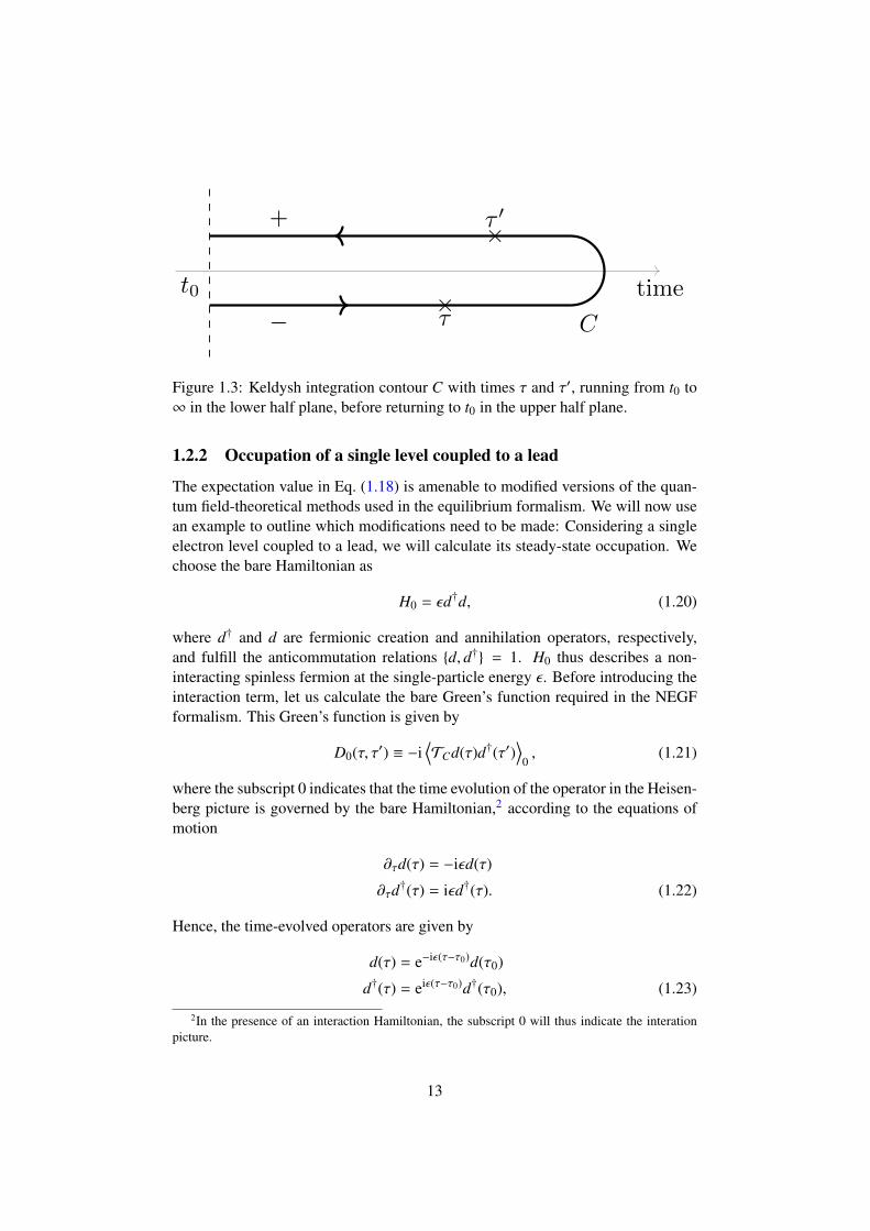
Figure 1.3: Keldysh integration contour C with times τ and τ′, running from t0 to∞ in the lower half plane, before returning to t0 in the upper half plane.
1.2.2 Occupation of a single level coupled to a lead
The expectation value in Eq. (1.18) is amenable to modified versions of the quan-tum field-theoretical methods used in the equilibrium formalism. We will now usean example to outline which modifications need to be made: Considering a singleelectron level coupled to a lead, we will calculate its steady-state occupation. Wechoose the bare Hamiltonian as
H0 = εd†d, (1.20)
where d† and d are fermionic creation and annihilation operators, respectively,and fulfill the anticommutation relations d, d† = 1. H0 thus describes a non-interacting spinless fermion at the single-particle energy ε. Before introducing theinteraction term, let us calculate the bare Green’s function required in the NEGFformalism. This Green’s function is given by
D0(τ, τ′) ≡ −i⟨TCd(τ)d†(τ′)
⟩0, (1.21)
where the subscript 0 indicates that the time evolution of the operator in the Heisen-berg picture is governed by the bare Hamiltonian,2 according to the equations ofmotion
∂τd(τ) = −iεd(τ)
∂τd†(τ) = iεd†(τ). (1.22)
Hence, the time-evolved operators are given by
d(τ) = e−iε(τ−τ0)d(τ0)
d†(τ) = eiε(τ−τ0)d†(τ0), (1.23)
2In the presence of an interaction Hamiltonian, the subscript 0 will thus indicate the interationpicture.
13
where the initial condition d(τ0) may remain unspecified here. The times τ and τ′
are defined on the contour C from Fig. 1.3. As a result of contour ordering, thevalue of D0(τ, τ′) depends on which of the two branches each of the times sits. TheGreen’s function in each of these four cases are commonly grouped together usingmatrix notation,3
D0(τ, τ′) =
(D−−0 (τ, τ′) D−+
0 (τ, τ′)D+−
0 (τ, τ′) D++0 (τ, τ′)
)=
−i⟨T d(τ)d†(τ′)
⟩0
i⟨d†(τ′)d(τ)
⟩0
−i⟨d(τ)d†(τ′)
⟩0−i
⟨T d(τ)d†(τ′)
⟩0
. (1.24)
The four components of D(τ, τ′) can be calculated using Eq. (1.22), for instance,
D−−0 (τ, τ′) = −i[θ(τ − τ′)
⟨d(τ)d†(τ′)
⟩0− θ(τ′ − τ)
⟨d†(τ′)d(τ)
⟩0
]= −ieiε(τ′−τ) [θ(τ − τ′)(1 − N0) − θ(t′ − t)N0
]= −ieiε(τ′−τ) [θ(τ − τ′) − N0
]. (1.25)
Here, the initial occupation number N0 was introduced, i.e.⟨d†(τ0)d(τ0)
⟩0≡ tr[ρ(t0)d†(τ0)d(τ0)] = N0, (1.26)
without making any assumptions about its value.4 The other three Green’s func-tions are obtained analogously,
D−+0 (τ, τ′) = ieiε(τ′−τ)N0
D+−0 (τ, τ′) = −ieiε(τ′−τ)(1 − N0)
D++0 (τ, τ′) = −ieiε(τ′−τ) [θ(t′ − t) − N0
]. (1.27)
Next, an interaction term is introduced as follows. Imagine the single particlepreviously modeled by H0 is coupled to a metallic lead, which is a system of manyeffectively non-interacting particles, with spatial extent L. We describe the lead bythe Hamiltonian
HB =∑
k
εkc†kck, (1.28)
where the index k enumerates the lead modes. Thus, we expand the bare Hamilto-nian to
H0 = εd†d +∑
k
εkc†kck. (1.29)
3occasionally referred to as a Keldysh matrix4Equivalently, the initial state ρ(t0) is unspecified.
14
The coupling of the single particle to the lead will be treated as an interaction,
V =∑
k
γk√
Ld†ck + h. c., (1.30)
with h. c. denoting the Hermitian conjugate. Each mode of the lead is coupled to thesingle particle with a time-independent tunneling amplitude γk. In the following,we quantify the effect of the coupling by calculating the contour-ordered Green’sfunction
D(τ, τ′) ≡ −i⟨TCd(τ)d†(τ′)
⟩, (1.31)
which differs from its bare counterpart in the fact that the expectation value iscalculated with respect to the Hamiltonian H = H0 + V . We employ the expressionfrom Eq. (1.18) to do so, expanding the interaction exponential in powers of V .After performing the leading-order expansion of D(τ, τ′), we have
D(τ, τ′) = −i⟨TCe
−i∫C dσ
[∑kγk√
Ld†(σ)ck(σ)+h.c.
]d(τ)d†(τ′)
⟩0
= D0(τ, τ′) −i2
∫C
dσ∫
Cdσ′
∑kq
[γkγ
∗q
L
⟨TCd†(σ)ck(σ)c†q(σ′)d(σ′)d(τ)d†(τ′)
⟩0
+γ∗kγq
L
⟨TCc†k(σ)c(σ)d†(σ′)cq(σ)d(τ)d†(τ′)
⟩0
]+ O(V4). (1.32)
Here, we assumed an initial state of the factorized form ρ(t0) = ρD(t0) ⊗ ρB(t0),meaning the coupling only affects the system as it starts to evolve. With this choice,the expectation values 〈cqd†〉0 and 〈c†qd〉0 both vanish, leading to the disappearanceof all odd-ordered terms in Eq. (1.32). Furthermore, we work with a thermal initialstate for the lead, ρB(t0) = e−βHB with an inverse temperature β = 1/T . Thisallows us to drop terms that will evaluate to zero because of 〈ckck〉 = 〈c†kc†k〉 = 0.In order to reduce the higher-order correlators in this expansion to products ofGreen’s functions, Wick’s theorem is employed, the validity of which extends tononequilibrium correlators [42]. This procedure results in
D(τ, τ′) = D0(τ, τ′) +
∫C
dσ∫
Cdσ′
∑k
γkγ∗k
LD0(τ, σ)G0,k(σ,σ′)D0(σ′, τ′)
+ O(V4), (1.33)
where we used the absence of off-diagonal correlators in the initial state ρB of thelead to drop the sum over q. Moreover, considerable simplification is brought aboutby the fact that fermion operators in contour-ordered expectation values freely an-ticommute. Eq. (1.33) does not just give the second-order result in perturbationtheory, but its structure also allows to deduce D(τ, τ′) to all orders: By iterating,we see that the exact Green’s function is obtained by substituting D(σ′, τ′) in place
15
= +
γ∗k γk+ . . .
D D(0) D(0) D(0)∑kαG
(0)kα
= +Σ
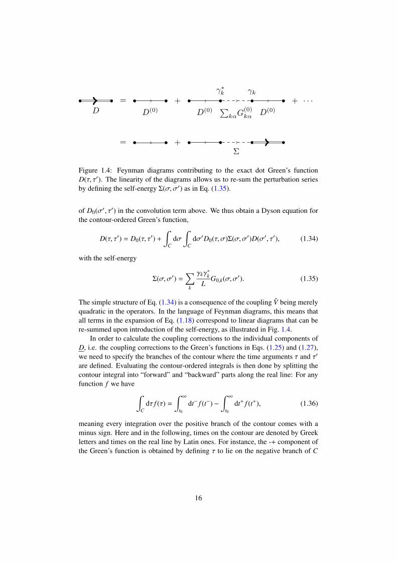
Figure 1.4: Feynman diagrams contributing to the exact dot Green’s functionD(τ, τ′). The linearity of the diagrams allows us to re-sum the perturbation seriesby defining the self-energy Σ(σ,σ′) as in Eq. (1.35).
of D0(σ′, τ′) in the convolution term above. We thus obtain a Dyson equation forthe contour-ordered Green’s function,
D(τ, τ′) = D0(τ, τ′) +
∫C
dσ∫
Cdσ′D0(τ, σ)Σ(σ,σ′)D(σ′, τ′), (1.34)
with the self-energy
Σ(σ,σ′) =∑
k
γkγ∗k
LG0,k(σ,σ′). (1.35)
The simple structure of Eq. (1.34) is a consequence of the coupling V being merelyquadratic in the operators. In the language of Feynman diagrams, this means thatall terms in the expansion of Eq. (1.18) correspond to linear diagrams that can bere-summed upon introduction of the self-energy, as illustrated in Fig. 1.4.
In order to calculate the coupling corrections to the individual components ofD, i.e. the coupling corrections to the Green’s functions in Eqs. (1.25) and (1.27),we need to specify the branches of the contour where the time arguments τ and τ′
are defined. Evaluating the contour-ordered integrals is then done by splitting thecontour integral into “forward” and “backward” parts along the real line: For anyfunction f we have ∫
Cdτ f (τ) =
∫ ∞
t0dt− f (t−) −
∫ ∞
t0dt+ f (t+), (1.36)
meaning every integration over the positive branch of the contour comes with aminus sign. Here and in the following, times on the contour are denoted by Greekletters and times on the real line by Latin ones. For instance, the -+ component ofthe Green’s function is obtained by defining τ to lie on the negative branch of C
16
and τ′ on the positive one. Using Eq. (1.36) to split the integrals yields
D−+(t, t′) = D−+0 (t, t′) +
∫ ∞
t0ds
∫ ∞
t0ds′D−−0 (t, s)Σ−−(s, s′)D−+(s′, t′)
−
∫ ∞
t0ds
∫ ∞
t0ds′D−+
0 (t, s)Σ+−(s, s′)D−+(s′, t′)
−
∫ ∞
t0ds
∫ ∞
t0ds′D−−0 (t, s)Σ−+(s, s′)D++(s′, t′)
+
∫ ∞
t0ds
∫ ∞
t0ds′D−+
0 (t, s)Σ++(s, s′)D++(s′, t′). (1.37)
Here, the components of the self energy are defined by taking the correspondingcomponent of G0,k(σ,σ′) in Eq. (1.35). This result, together with the other threecomponents, can be written more compactly in terms of matrices along the lines ofEq. (1.24),
D(t, t′) = D0(t, t′) +
∫ ∞
t0ds
∫ ∞
t0D0(t, s)Σ(s, s′)D(s′, t′). (1.38)
Note that the self-energy matrix is defined so as to include the negative signs arisingfrom the contour integration,
Σ(s, s′) =
(Σ−−(s, s′) −Σ−+(s, s′)−Σ+−(s, s′) Σ++(s, s′)
). (1.39)
When calculating transport properties of a system below, we will also make use ofthe retarded and advanced Green’s functions. These are defined by
DR(t, t′) ≡ −iθ(t − t′)⟨c(t), c†(t′)
⟩,
DA(t, t′) ≡ iθ(t′ − t)⟨c(t), c†(t′)
⟩=
[DR(t′, t)
]∗, (1.40)
(1.41)
respectively. It is easily verified how these Green’s functions are related to theprevious definitions,
DR(t, t′) = D−−(t, t′) − D−+(t, t′)
DA(t, t′) = D−−(t, t′) − D+−(t, t′). (1.42)
These Green’s functions play a central role, among other things, in determiningthe excitation spectrum of a system and its response to external influences. Onthe other hand, information about its distributional properties is encoded in D−+
and D+−, which are often referred to as the lesser and greater Green’s functions,respectively. As an alternative, these properties can be summarized in the so-calledkinetic (or Keldysh) Green’s function
DK(t, t′) = D−+(t, t′) + D+−(t, t′). (1.43)
17
In the following, we modify the matrix Green’s function by employing a commonprocedure known as Keldysh rotation,
D =
(DR DK
0 DA
)= LσzDL†, (1.44)
where L denotes the Hermitian matrix
L ≡1√
2
(1 −11 1
), (1.45)
and
σz =
(1 00 −1
)(1.46)
is the third Pauli matrix. Using this convention, we obtain the Dyson equation
D(t, t′) = D0(t, t′) +
∫ ∞
t0ds
∫ ∞
t0ds′D0(t, s)Σ(s, s′)D(s′, t′). (1.47)
Here, the self-energy is given by
Σ(s, s′) =
(ΣR(s, s′) ΣK(s, s′)
0 ΣA(s, s′)
), (1.48)
meaning there are no additional minus signs as in Eq. (1.39). In particular, thetriangular shape of all matrices in Eq. (1.47) implies that the coupling correctionsto the retarded and advanced Green’s function can be calculated using only thecorresponding components of G0 and Σ,
DR/A(t, t′) = DR/A0 (t, t′) +
∫ ∞
t0ds
∫ ∞
t0ds′DR/A
0 (t, s)ΣR/A(s, s′)DR/A(s′, t′).
(1.49)
Let us also give the Dyson equations for the lesser and greater Green’s functions,
D∓±(t, t′) = D∓±0 (t, t′) +
∫ ∞
t0ds
∫ ∞
t0ds′DR
0 (t, s)ΣR(s, s′)D∓±(s′, t′)
+
∫ ∞
t0ds
∫ ∞
t0ds′DR
0 (t, s)Σ∓±(s, s′)DA(s′, t′)
+
∫ ∞
t0ds
∫ ∞
t0ds′D∓±0 (t, s)ΣA(s, s′)DA(s′, t′), (1.50)
which arises in analogous fashion to the kinetic component of Eq. (1.47). Eq. (1.50)is an application of the Langreth rule [46, 47], which relates the lesser component
18
of a convolution to convolutions of the constituents’ components: Given the func-tion C(τ, τ′) =
∫C dσA(τ, σ)B(σ, τ′), rewriting the contour integrals as real ones
according to Eq. (1.36) results in the identity
C±∓(t, t′) =
∫ ∞
t0ds
[AR(t, s)B±∓(s, t′) + A±∓(t, s)BA(s, t′)
]. (1.51)
A straightforward application of the lesser Green’s function lies in computingthe particle number
N(t) ≡⟨d(t)d†(t)
⟩= −iD−+(t, t). (1.52)
Often, one is interested in the situation of the steady state of the system, wherethe effects characterizing the regime close to the initial state have died out andthe asymptotic behavior has established itself, with N(t) having converged to itssteady-state value. In the NEGF formalism for a time-independent Hamiltonian,this is achieved by moving the initial time into the infinite past, t0 → −∞. Wefurthermore expect that all Green’s functions in this situations will only depend onrelative times, so we make the ansatz D−+(t, t′) = D−+(t − t′). Then, the Dysonequation (1.50) for D−+ can be written in terms of convolutions,
D−+(t − t′) = D−+0 (t − t′) +
[DR
0 ∗ ΣR ∗ D−+]
(t − t′)
+[DR
0 ∗ Σ−+ ∗ DA]
(t − t′) +[D-+
0 ∗ ΣA ∗ DA]
(t − t′), (1.53)
where convolution of two functions A and B is defined as
[A ∗ B](t) =
∫ ∞
−∞
dsA(s)B(t − s). (1.54)
By considering the Fourier-transformed Green’s function,
D−+(ω) =
∫ ∞
−∞
d(t)eiωtD−+(t), (1.55)
the convolutions are replaced by products, and iteration of Eq. (1.53) yields
D−+(ω) = (1 + DR(ω)ΣR(ω))D−+0 (ω)(1 + DA(ω)ΣA(ω)) + DR(ω)Σ−+(ω)DA(ω),
(1.56)
where the Fourier transform of Eq. (1.49) was used,
DR/A(ω) = DR/A0 (ω) + DR/A
0 (ω)ΣR/A(ω)DR/A(ω). (1.57)
D−+(ω) simplifies considerably upon introduction of the Fourier transformed initialGreen’s functions,
D−+0 (ω) = i2πδ(ω − ε)N0
DR0 (ω) =
1ω − ε + iη
, (1.58)
19
where N0 denotes the initial occupation number of the level, and the positive in-finitesimal η → 0 encodes the time retardation in frequency space. By applyingthe Fourier transform of Eq. (1.49) to the first factor of the first term in Eq. (1.56),one obtains
D−+(ω) =DR
0 (ω)−1
DR0 (ω)−1 − ΣR(ω)
D−+0 (ω)(1 + DA(ω)ΣA(ω)) + DR(ω)Σ−+(ω)DA(ω)
(1.59)
Since Eq. (1.58) implies DR0 (ω)−1D−+
0 (ω) = 0, the first term evaluates to zero andwe are left with
D−+(ω) = DR(ω)Σ−+(ω)DA(ω). (1.60)
Hence, the occupation of the level in the infinite past has no effect on the steady-state solution for D−+, which can be obtained from the retarded and advancedsolutions of Eq. (1.57),
DR/A(ω) =1
DR/A0 (ω)−1 − ΣR/A(ω)
=1
ω − ε − ΣR/A(ω). (1.61)
The retarded and advanced components of the self-energy is given by
ΣR/A(ω) =∑
k
γ∗kγk
L1
ω − εk ± iη= P
∑k
γ∗kγk
L1
ω − εk∓ iπ
∑k
γ∗kγk
Lδ(ω − εk)
≡ Λ(ω) ∓ iΓ(ω), (1.62)
with the negative and positive signs in the last line applicable for the retarded andadvanced components, respectively. The real part, commonly denoted Λ(ω), ef-fects a Lamb shift in the location of the peak of DR(ω), and the imaginary partΓ(ω) describes the broadening of the particle linewidth as a result of coupling it tothe lead. This imaginary part serves to regularize the denominator in Eq. (1.61),replacing the infinitesimal η. The lesser self-energy is proportional to the linewidthand the distribution function of the lead,
Σ−+(ω) =∑
k
γ∗kγk
LG−+
0,k (ω) = 2πi∑
k
γ∗kγk
LnF(εk)δ(ω − εk) = i2nF(ω)Γ(ω). (1.63)
Finally, the pieces can be assembled and the steady state particle number is givenby
Nss =
∫dω2π
D−+(ω) =
∫dω2π
2Γ(ω)(ω − ε − Λ(ω))2 + Γ2(ω)
nF(ω). (1.64)
In summary, the effects of coupling to the particle to the lead and taking the steady-state limit are (i) level broadening leading to a finite linewidth Γ, (ii) energy shiftby Λ, and (iii) thermalization according to the lead distribution nF.
20
εL R
...
...
εkR
...
...
εkL
γkRγkL
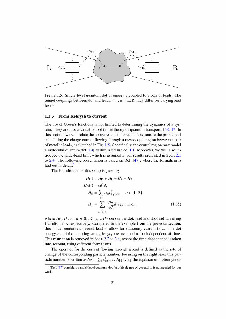
Figure 1.5: Single-level quantum dot of energy ε coupled to a pair of leads. Thetunnel couplings between dot and leads, γkα, α = L,R, may differ for varying leadlevels.
1.2.3 From Keldysh to current
The use of Green’s functions is not limited to determining the dynamics of a sys-tem. They are also a valuable tool in the theory of quantum transport. [48, 47] Inthis section, we will relate the above results on Green’s functions to the problem ofcalculating the charge current flowing through a mesoscopic region between a pairof metallic leads, as sketched in Fig. 1.5. Specifically, the central region may modela molecular quantum dot [19] as discussed in Sec. 1.1. Moreover, we will also in-troduce the wide-band limit which is assumed in our results presented in Secs. 2.1to 2.4. The following presentation is based on Ref. [47], where the formalism islaid out in detail.5
The Hamiltonian of this setup is given by
H(t) = HD + HL + HR + HT,
HD(t) = εd†d,
Hα =∑
k
εkαc†kαckα, α ∈ L,R
HT =∑
kα=L,R
γkα√
Ld†ckα + h. c., (1.65)
where HD, Hα for α ∈ L,R, and HT denote the dot, lead and dot-lead tunnelingHamiltonians, respectively. Compared to the example from the previous section,this model contains a second lead to allow for stationary current flow. The dotenergy ε and the coupling strengths γkα are assumed to be independent of time.This restriction is removed in Secs. 2.2 to 2.4, where the time-dependence is takeninto account, using different formalisms.
The operator for the current flowing through a lead is defined as the rate ofchange of the corresponding particle number. Focusing on the right lead, this par-ticle number is written as NR =
∑k c†kRckR. Applying the equation of motion yields
5Ref. [47] considers a multi-level quantum dot, but this degree of generality is not needed for ourwork.
21
the current,
IR(t) ≡ e∂tNR = ie[H,NR] = ie∑
k
γkR√
Ld†ckR + h. c. . (1.66)
In order to calculate the expectation value of this operator, we introduce the mixedGreen’s functions
Fkα(τ, τ′) ≡ −i⟨TCckα(τ)d†(τ′)
⟩. (1.67)
Taking the lesser component enables us to write
〈IR(t)〉 = 2e Re∑
k
γkR√
LF−+
kR (t, t). (1.68)
The calculation of the current thus reduces to the calculation of the mixed Green’sfunctions. In order to relate these with the Green’s functions introduced previously,we assign to HT the role of the interaction Hamiltonian and consider the contourS-matrix
S C = TCe−i∫C dτHT(τ). (1.69)
The perturbation expansion of Fkα(τ, τ′) is thus given by
Fkα(τ, τ′) = −i⟨TCe−i
∫C dσHT(σ)ckα(τ)d†(τ′)
⟩0
= −i⟨TC
∑j≥0
(−i) j
j!
∫C
dσ
∑kα
γkα√
Ld†(σ)ckα(σ) + h. c.
j
ckα(τ)d†(τ′)⟩
0
.
(1.70)
Using Wick’s theorem, as well as 〈d†ck〉0 = 〈c†kd〉0 = 〈ckcq〉0 = 〈c†kc†q〉0 = 0, wesee that the terms of the expansion can be regrouped, leading to
Fkα(τ, τ′) =
∫C
dσG0,kα(τ, σ)γ∗kα√
LD(σ, τ′), (1.71)
where the dot and bare lead Green’s functions are defined as before,
D(τ, τ′) = −i⟨TCd(τ)d†(τ′)
⟩,
G0,kα(τ, τ′) = −i⟨TCckα(τ)c†kα(τ′)
⟩0, (1.72)
respectively. G0,kα denotes the bare lead Green’s function for the lead of index α.As in Sec. 1.2.2, we study the steady-state situation by taking the limit of t0 → −∞.Substitution of D(τ, τ′) into Eq. (1.68) yields for the current through the right lead
〈IR(t)〉 = 2e Re∫ ∞
−∞
ds[ΣR
R(t, s)D−+(s, t) + Σ−+R (t, s)DA(s, t)
], (1.73)
22
where the self-energy now also contains a summation over the leads,
ΣR(s, s′) =∑kα
γ∗kαγkα
LGR
0,kα(s, s′). (1.74)
The summation over lead modes can be simplified by taking the wide-band limit(WBL), presuming that the coupling γα to the leads does not depend on the individ-ual lead mode k, and that the density of states ρ in the leads is constant throughoutthe relevant range of energies.6 The latter is equivalent to linearizing the lead spec-trum, εkα = vFk near the Fermi surface, with the constant Fermi velocity vF. Usingthese simplifications, the contribution of lead α to the retarded self-energy evalu-ates to
ΣRα(s, s′)WBL
= − iγ∗αγα
Lθ(s − s′)
∑k
e−iεkα(s−s′)
= −iργ∗αγαθ(s − s′)∫
dωe−iω(s−s′)
= −iΓαδ(s − s), (1.75)
where we introduced the tunneling rate Γα = |γα|2/(2vF). The density of states was
used in the form
ρ =∑
k
δ(ω − εkα)/L =1
2πvF(1.76)
to convert the sum over modes∑
k /L into the frequency integral ρ∫
dω. The thetafunction contributes a factor of θ(0) = 1/2. Comparing to Eq. (1.62), we note thatas a result of taking the WBL, ΣR is purely imaginary and delta-shaped in the timedomain. In the same way, the lesser component is obtained,
Σ−+α (s, s′)WBL
= iγ∗αγα
L
∑k
e−iεkα(s−s′)nF(εk)
= iργ∗αγα
∫dωe−iω(s−s′)nFα(ω). (1.77)
This frequency integral features an unphysical divergence as a result of the infinitebandwidth in the WBL. It can be cured by introducing a frequency cutoff, but wewill in general not make this procedure explicit in the following.
As in Sec. 1.2.2, the steady-state current is obtained by making an ansatz forD−+ that only depends on time differences. In the frequency domain, the lesser dotGreen’s function is then
D−+(ω) = DR(ω)[Σ−+
L (ω) + Σ−+R (ω)
]DA(ω). (1.78)
6The WBL is known to be accurate for metallic electrodes, where the temperature is small com-pared to the Fermi energy. Further remarks on its validity can be found in Ref. [49].
23
In particular, this implies D−+(t) = −D−+(−t)∗, and therefore, in the steady state,after substituting Eqs. (1.75) and (1.77), Eq. (1.73) simplifies to
〈IR〉ss = −i2eΓR
∫dω2π
[D−+(ω) + nFR(ω)(DR(ω) − DA(ω))
]. (1.79)
In the steady state, one needs to impose 〈IR〉ss = − 〈IL〉ss in order to exclude solu-tions with infinite charge accumulation on the dot. The current can then be writtenas 〈I〉ss = (〈IR〉ss − 〈IL〉ss)/2. In the case of ΓL = ΓR, the term proportional toD−+(ω) in Eq. (1.79) drops out, giving the final result for the WBL steady-statecurrent
〈I〉ss = ieΓ
2
∫dω2π
[nFL(ω) − nFR(ω)][DR(ω) − DA(ω)
]. (1.80)
The most striking feature of this current is that it only depends on the retarded dotGreen’s function, and its frequency domain is defined by the “window” nFL − nFRin the lead distributions.
24

1.3 Floquet expansion for driven systems
Driven quantum systems have long been a mainstay of quantum physics in gen-eral and transport theory in particular [50, 51, 52]. Accordingly, a wide array ofanalytical and numerical techniques has been developed for their analysis. Givena system described by a time-dependent Hamiltonian, there is no single, feasible,technique to obtain the system dynamics for a completely general drive. Rather,the choice of method depends strongly on the manner of driving the system, for in-stance a slow drive may be treated in the adiabatic approximation, or a weak drivemay be amenable to perturbation theory. For a periodic drive without restriction onits speed or strength, the Floquet approach has proven successful.
Here, we give an overview of the Floquet technique in preparation for Sec. 2.2,where it is applied to a molecular quantum dot with a periodic driving force. Origi-nating from the theory of differential equations [53, 54], the Floquet technique canbe used to treat periodic Hamiltonians,
H(t + T ) = H(t) ∀t. (1.81)
In this case, the Schrodinger equation i∂tφ(t) = H(t)φ(t) admits a complete set ofsolutions of the form
φα(t) = e−iEαtuα(t), (1.82)
where uα inherits the periodicity of the Hamiltonian, and hence admits a decom-position in harmonics of the drive frequency Ω = 2π/T ,
uα(t + T ) = uα(t) =∑n∈Z
e−inΩtunα. (1.83)
The Eα in Eq. (1.82) are known as quasi-energies. The decomposition in Eq. (1.83)implies that the quasi-energies are only defined up to integer multiples of the drivefrequency. Indeed, by shifting the energy one finds
e−i(Eα+kΩ)tuα(t) = e−iEαt∑n∈Z
e−i(n−k)Ωtunα = e−iEαt∑n∈Z
e−inΩtu(n+k)α, (1.84)
which is also a solution of the Schrodinger equation. Hence the range of the quasi-energies can be restricted to 0 ≤ Eα < Ω, analogously to the emergence of theBrillouin zone in systems with spatial periodicity. This leads to the interpreta-tion of the exponential e−iEαt describing the long-time (low-energy) behavior ofthe wave function, whereas the periodic factor uα(t) encodes its evolution on timescales shorter than the drive period. By decomposing the Schrodinger equationinto Fourier components, an equation for the mode amplitudes unα is obtained,∑
n∈Z
Hmnunα = (Eα + mΩ)umα, (1.85)
25
meaning that the time-dependent problem can be mapped onto a time-independentone involving an infinite-matrix Hamiltonian with entries
Hmn =1T
∫ T/2
−T/2dtei(m−n)ΩtH(t). (1.86)
This representation of the Schrodinger equation suggests interpreting the role ofthe drive as a source of “photons” of frequency Ω.
An analogous formalism can also be developed in the language of Green’sfunctions, as was laid out in Ref. [55]: Consider a general NEGF G(t, t′), where thecheck mark indicates the 2 × 2 matrix structure with both times defined on the realline, using the notation from Sec. 1.2. First, time dependence can be expressed interms of the relative and average times trel = t− t′, and tav = (t + t′)/2, respectively.Then, a Fourier transform is performed in the relative coordinate,
D(tav, ω) =
∫ ∞
−∞
dtreleiωtrel D(tav, trel). (1.87)
As a consequence of the periodicity of the Hamiltonian, the Green’s function isitself periodic in the average time if initial state effects are disregarded. Hence itcan be expanded into Fourier modes,
D(n, ω) =1T
∫ T/2
−T/2dtaveinΩtav D(tav, ω). (1.88)
Having performed this expansion, the Green’s function can be written as an infinite-dimensional Floquet matrix in frequency space,
Dmn(ω) = D(m − n, ω +
m + n2
Ω
). (1.89)
This matrix representation allows to write convolutions in time domain as matrixmultiplications in frequency space: For a function
C(t, t′) =
∫ ∞
−∞
dsA(t, s)B(s, t′), (1.90)
the Floquet expansion is given by
Cmn(ω) =
∞∑k=−∞
Amk(ω)Bkn(ω). (1.91)
In order to calculate this matrix product numerically, it is necessary to make an ap-proximation, the most simple one being to only take a finite number NFl of Floquetmodes into account. This corresponds to limiting the dimension of the matrices toN ≡ 2NFl + 1, with the index k running from −NFl to NFl.
26
1.4 Open quantum systems and master equations
Only very rarely do quantum systems occur in complete isolation from their sur-roundings. This is true especially in the context of transport theory, where systemsare embedded in environments in order to induce a current flowing through them.More generally, a quantum system will almost invariably interact with its surround-ings in some way, leading to various consequences such as hybridization of energylevels, particle loss, or dissipation of energy. Typically, the environment in sucha setup contains a macroscopic number of degrees of freedom and allows for lessexperimental control than the system itself, making it very challenging to describewith an exact quantum model. Moreover, the environment is usually only of inter-est by virtue of how it affects the system, so the environment dynamics themselvestend to be of lesser relevance.
1.4.1 From von Neumann to Lindblad
The notion of an open system encompasses any quantum system in contact withan environment. In this situation, it has in many cases proven possible to obtain aneffective description for the dynamics of the open system in which the environmentdegrees of freedom no longer occur as variables. Since the resulting model onlycontains the system degrees of freedom, it can be much easier to treat, while stillpreserving information about the effects of the environment on the system. Con-figurations with weak coupling between system and environment are particularlyamenable to such an approach. In the following, we will sketch the derivation of aneffective model that will prove useful in corroborating our results from the NEGFapproach, in Sec. 2.1.
Since the form and eventual tractability of such an effective model for the opensystem will in any case depend on the configuration in question, we do not aimfor generality here, but will instead focus on what is used in Sec. 2.1. The mainreference used here is Ch. 6 of Ref. [56], others include the textbooks [57, 58]. Arigorous treatment can be found in Ref. [59].
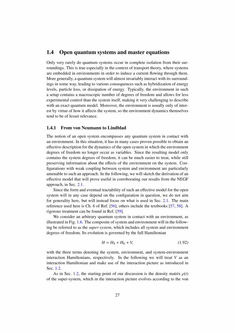
We consider an arbitrary quantum system in contact with an environment, asillustrated in Fig. 1.6. The composite of system and environment will in the follow-ing be referred to as the super-system, which includes all system and environmentdegrees of freedom. Its evolution is governed by the full Hamiltonian
H = HS + HE + V, (1.92)
with the three terms denoting the system, environment, and system-environmentinteraction Hamiltonians, respectively. In the following we will treat V as aninteraction Hamiltonian and make use of the interaction picture as introduced inSec. 1.2.
As in Sec. 1.2, the starting point of our discussion is the density matrix ρ(t)of the super-system, which in the interaction picture evolves according to the von
27
Super-system
System Environment
ρH
ρSHS
HEV
Figure 1.6: Schematic representation of an open system in contact with an envi-ronment. The open system dynamics are encoded in the reduced density matrixρS, which exclusively retains the system degrees of freedom. The time evolutionof ρS is obtained by evolving the density matrix ρ of the super-system with the fullHamiltonian H = HS + HE + V and then tracing over the environment degrees offreedom.
Neumann equation
ddtρ(t) = −i[V , ρ(t)]. (1.93)
We aim to find an expression for the reduced density matrix ρS(t), which is obtainedfrom ρ(t) by tracing over the environment degrees of freedom,
ρS(t) = trE ρ(t). (1.94)
A simplified equation of motion for ρS (as opposed to ρ) can be obtained fromEq. (1.93), given certain assumptions. First, the super-system is required to be ina factorized state ρ(t0) = ρS(t0) ⊗ ρB at the initial time t0. Here, ρB is a fixed stateof the environment, often taken to be a thermal state ρB = e−βHE/ tr e−βHE at aninverse temperature β. In this case, the environment is referred to as a bath, asindicated by the index B. Second, the coupling between system and environment isassumed to be weak, and that the dynamics of the bath are much faster than thoseof the system. Under these assumptions, the von Neumann equation can be shownto imply
ρS(t) = ρS(t0) −∫ t
t0ds
∫ s
t0du trE
[V(s),
[V(s − u), ρS(s) ⊗ ρB
]]+ O(V3), (1.95)
28
where the interaction picture with respect to HS + HE is indicated by hats. By mak-ing some further assumptions about the correlators of the environment operators inthe interaction Hamiltonian V ,7 it is possible to arrive at a linear master equationfor ρS,
dρS(t)dt
= −i[HLS, ρS(t)] +D[ρS(t)
], (1.96)
where HLS contributes a shift of the system energy levels due to the coupling tothe bath and is hence referred to as the Lamb-shift Hamiltonian. The operatorD iscalled a dissipator, and its action on the system density matrix is given by
D[ρS
]=
∑µ
∑ω
γµ(ω)(Cµ(ω)ρSC†µ(ω) −
12
C†µ(ω)Cµ(ω), ρS
), (1.97)
where the operators Cµ represent various decay channels, and the sum over ω cor-responds to adding contributions from the entire spectrum of the system. Eq. (1.96)is known as the Lindblad equation [59] for the system density matrix and capturesthe non-unitary part of the evolution of the system resulting from the contact withthe bath.
1.4.2 A note on Markovianity
In the context of open system dynamics, a commonly used notion is that of Marko-vian evolution. Specifically, the Lindblad equation (1.96) is usually taken to indi-cate that the system evolves in a Markovian manner. The exact meaning of Marko-vianity is however more complex than this would suggest. A considerable amountof literature is dedicated to the issue, see Refs. [60, 56, 61, 62] among others; here,we borrow from Refs. [57, 56] and establish the main points in as far as will beneeded to provide context for our own work.
The origin of the term lies in classical probability theory, where a stochasticprocess, i.e. a sequence (Xn)n∈N of random variables is called Markovian, if thedistribution of any element in the sequence only depends on its immediate prede-cessor,
P(Xn = x|Xn−1 = xn−1, . . . , X0 = x0) = P(Xn = x|Xn−1 = xn−1), (1.98)
where P(A|B) ≡ P(A ∩ B)/P(B) denotes the probability of the event A conditionedon the event B. This property is a manifestation of the process being memoryless,i.e. the transition probabilities between the nth and (n−1)st steps do not depend onthe history of the process. This notion is readily generalized to continuous stochas-tic processes (Xt)t∈I . There, denoting by p(x, t) the probability for the process totake the value x at the time t, we have by definition
p(x, t) =
∫dx′p(x, t|x′, t′)p(x′, t′) ∀t′ < t, (1.99)
7These assumptions are related to, but not equivalent to assuming an infinite number of environ-ment degrees of freedom. For details, see Ch. 6 of Ref. [56].
29
where the conditional probability p(x, t|x′, t′) acts as a transition kernel for theevolution between t′ and t. The Markov condition is formulated in analogy toEq. (1.98), and imposed for any sequence of times, for example p(x3, t3|x2, t2, x1, t1) =
p(x3, t3|x2, t2). This implies a composition law for the transition kernel,
p(x3, t3|x1, t1) =
∫dx2 p(x3, t3|x2, t2)p(x2, t2|x1, t1), (1.100)
for all intermediate times t1 < t2 < t3, known as the Chapman-Kolmogorov equa-tion.
The quantum version of Markovianity can be introduced by drawing uponEq. (1.100) and requiring a similar composition rule. More precisely, the role ofthe probabilities p(x, t) is taken by the system density matrix ρS(t). Given a fac-torized initial state ρ(t0) = ρS(t0) ⊗ ρB of the super-system, it is possible to finda family of linear operators E(t) that encode the evolution of the reduced densitymatrix ρS(t) = trB ρ(t),
ρS(t0 + t) = E(t)[ρS(t0)
](1.101)
in such a way it fulfills a composition law analogous to Eq. (1.100). Since theenvironment degrees have already been traced out, the evolution of ρS(t) is notunitary and hence does not inherit the group property of the propagator U(t, t′) ofthe super-system. Nonetheless, by introducing the spectral decomposition ρB =∑β λβ |φβ〉 〈φβ| of the initial bath density matrix, it is possible to write the evolution
of ρS as
ρS(t0 + t) = trB[U(t0 + t, t0)ρS(t0) ⊗ ρBU†(t0 + t, t0)
]=
∑α
〈φα|U(t0 + t, t0)ρS(t0) ⊗
∑β
λβ |φβ〉 〈φβ|
U†(t0 + t, t0) |φβ〉
≡∑αβ
W†αβ(t)ρS(t0)Wαβ(t), (1.102)
where Wαβ =√λβ 〈φα|U(t0 + t, t0) |φβ〉. This expression is of the form from
Eq. (1.101), with
E(t) [·] =∑αβ
W†α(t)[·]Wβ(t) (1.103)
denoting the trace-preserving evolution operator for the reduced density matrix.The analogy to Eq. (1.100) is constructed by imposing the semigroup condition
E(t + s) = E(t)E(s) ∀t, s ≥ 0. (1.104)
If this condition is fulfilled and E(t) is in addition completely positive,8 then E issaid to model a Markovian process. It can be shown that the evolution of a density
8A map Emapping operators to operators is called positive if it maps positive operators to positiveoperators, i.e. operators with only positive eigenvalues. E is called completely positive if for anypositive operator ρ also the operators 1d ⊗ E[ρ] are positive, for any dimension d.
30
matrix ρS by E(t) can equivalently be described by the equation
ddtρS = −i[H, ρS] +
N2−1∑µ=1
hµ
(CµρSC†µ −
12
C†µCµ, ρS
), (1.105)
with positive coefficients hµ ≥ 0. The integer N denotes the dimension of thesystem Hilbert space, which is assumed to be finite in this context. It should bestressed that the operator H is a function of bath expectation values of the super-system evolution operator U(t, t0), and does in general not coincide with the systemHamiltonian HS. Eq. (1.105) is of the same form as Eq. (1.96), showing that theapproximations performed in Sec. 1.4.1 do indeed lead to a notion of quantumMarkovianity. However, this is far from the only such notion and many alternativedefinitions exist, an overview of which can be found in Ref. [62].
31
1.5 Quantum thermodynamics: An overview
Thermodynamics and quantum mechanics are two of the most consequential para-digms in modern science. Their fields of application have historically been sep-arated by massive differences in scale: Classical thermodynamics describes theinterplay between macroscopic systems and is used to design macroscopic ma-chines and work cycles. Quantum mechanics, on the other hand, concerns itselfwith microscopic particles and processes. Even though the laws of thermodynam-ics can be seen to arise from quantum mechanics, their domain of validity is onlyreached by taking the thermodynamic limit of quasi-infinite particle number N. Asa general rule of thumb, particle numbers on the macroscale are on the order ofAvogadro’s constant, NA ≈ 6 × 10²³, and classical thermodynamics is furthermoreonly of limited use beyond equilibrium. Hence, it took decades after the discov-ery of quantum mechanics for the question of quantum thermodynamics to attractconsiderable attention. More recently, fabrication techniques have improved to thepoint where meso- and nanoscale machines can be reliably realized in experiments,leading to a surge in interest in the topic: On the single-particle scale [63, 64, 65],the thermodynamic limit can evidently not be taken. On the mesoscale, the particlenumber may still be quite sizable (up to 1012 particles), but other assumptions ofthe classical theory break down nonetheless. In this section, we will outline thesefundamental issues of quantum thermodynamics as well as some of the establishedresults, in as far as they are connected to the work in Secs. 2.3 and 2.4.
The central question in quantum thermodynamics can be formulated as How dothe macroscopic laws of classical thermodynamics generalize to hold in quantumsystems? These laws of thermodynamics can be formulated as follows [66]:
1. Infinitesimal changes in the internal energy of a system (dES) are the sum ofheat flowing into the system (δQ), work performed on it (δW), and changesin chemical energy (δEC),
dES = δQ + δW + δEC, (1.106)
where d in contrast to δ indicates a complete differential, meaning that theinternal energy of a system is a state function, whereas heat, work, and chem-ical energy in general are not.
2. A process that adds the heat δQ to a system at temperature T causes thechange of entropy
dS ≥δQT. (1.107)
3. Entropy changes incurred during isothermal processes vanish in the limit ofthe temperature tending to zero.
The focus of this work lies on the first two laws. The first law is a statement ofenergy conservation, which clearly also holds in quantum mechanics. The chal-lenge however consists in finding definitions of system energy, work and heat that
32
not only fulfill the first law, but also the other two. In order to retain maximumgenerality, these definitions moreover need to be made with as little reference aspossible to a specific model. The second law relates the heat flux δQ during a workcycle with the entropy increase, which is also in need of a definition. Again, thedefinition should be made in such a manner that the law holds for arbitrary systemsand work protocols, in analogy to the vast generality of classical thermodynamics.
Some of the roadblocks on the way to a consistent theory of quantum ther-modynamics are readily apparent: Firstly, in classical thermodynamics, the exactnature of the interaction between reservoirs and systems is not taken into account.This simplification results from the fact that at macroscopic scales, the interfacesbetween systems only occupy negligible space and thus do not significantly modifythe energy balance. For quantum systems containing only a few particles, this as-sumption no longer holds, leading to a conflict between the goal of generality andthe need to treat interaction effects explicitly. If these interactions are strong, aneven more fundamental concern arises, namely which part of an interface belongsto which system. Considering this issue, it is perhaps not surprising that quantumthermodynamics of weakly coupled system has proved to be the more accessibleproblem, and a satisfactory theory has emerged decades ago [67, 68, 9, 69]. Theformalism of open quantum systems, as described in Sec. 1.4, is instrumental inthis endeavor, which we outline below, following Ref. [9].
1.5.1 Open quantum systems and weak-coupling thermodynamics
Consider the reduced density matrix for an open system with a driven HamiltonianHS(t) weakly coupled to a bath, which evolves in Markovian fashion,
ddtρS(t) = −i[HS(t), ρS(t)] +Dt[ρS(t)], (1.108)
where the time-dependence of HS(t) is only parametrical, and Dt is calculatedfrom HS(t) according to Eq. (1.97), indicating that the Hamiltonian is driven insuch a way that the dynamics of the reduced density matrix are still described bya Lindblad equation. In this setting, thermodynamic quantities can be defined thatrelate to the notions of macroscopic thermodynamics. Specifically,
ES(t) = tr (ρS(t)HS(t)) ,
Q(t) = tr(
ddtρS(t)HS(t)
),
W(t) = tr(ρ(t)
ddt
HS(t))
(1.109)
are used to denote the internal energy of the system, the rate of heat flowing into it,and the rate of work it performs, respectively. Here, we introduce the convention ofindicating time derivatives by using ∂t, and giving a dot to quantities that describea rate, but need not actually be time derivatives of a state function. These choices
33
fulfill ∂tES(t) = W + Q, which generalizes the first law from Eq. (1.106) to thequantum case in a straightforward fashion. Defining the von Neumann entropywith the system density matrix,
S S(t) = − tr[ρS(t) log ρS(t)
](1.110)
it can be shown that the rate of change of entropy is given by
∂tS (t) = βQ(t) + S i(t), (1.111)
where the first term describes the entropy flow into the system, and the second oneis the entropy production rate in the system, which is found to be positive,
S i(t) ≥ 0. (1.112)
This result amounts to a quantum version of the second law, Eq. (1.107). It shouldbe stressed that the derivation of Eq. (1.112) hinges on the Markovian evolution onthe system density matrix as encoded in the Lindblad equation (1.105), and hencein particular on the weakness of the coupling between system and bath.
In the regime of strong system-bath coupling, no universal formulation of quan-tum thermodynamics exists. There are however several approaches each capturingsome aspects of quantum thermodynamics, of which we want to give an overviewnow.
1.5.2 Stochastic thermodynamics
Stochastic thermodynamics has its roots in nonequilibrium classical thermodynam-ics and has proven fruitful with in the study of work in the quantum case. Its start-ing point is provided by a result of Jarzynski [70] about a classical system initiallyweakly coupled by a Hamiltonian HT to a heat bath with Hamiltonian HB, equi-librated at an inverse temperature β. After this initial time, the bath is decoupledand the system is modeled by a Hamiltonian Hλ(z), where λ(t) = t/t f denotes thecontrol parameter used in a switching protocol and z = (q, p) is shorthand for a co-ordinate in the system phase space. The evolution of the system is then describedby the stochastic trajectory z(t) in phase space, where t ranges between initial andfinal times t0 and t f , and the work performed along this trajectory is
W =
∫ t f
t0dtλ(t)∂λHλ(z(t)). (1.113)
The average work 〈W〉 is obtained by averaging Eq. (1.113) over the initial config-urations of the super-system consisting of system and bath. In the case of an initialthermal state at inverse temperature β, it can be shown that the average exponenti-ated work is equal to the exponentiated free energy difference,⟨
e−βW⟩
= e−β∆F , (1.114)
34
with ∆F = F(t f ) − F(t0), where the initial equilibrium free energy is defined as
F(t0) = −1β
log Z(t0), (1.115)
with the classical partition function
Z(t0) =
∫dzdz′e−β(H0(z)+HB(z′)+HT(z,z′)). (1.116)
where z′ denotes the phase space coordinates of the bath. The final equilibriumfree energy F(t f ) is defined analogously. The result Eq. (1.114), named Jarzynski’sequality, establishes an equality between the average of a non-equilibrium quantityand a change of an equilibrium thermodynamic potential. The equilibrium freeenergy is thus accessible by averaging over nonequilibrium work measurements.Since the inverse exponential function is concave, Jensen’s inequality implies
〈W〉 ≥ ∆F, (1.117)
meaning Jarzynski’s equality can also be seen as a stronger, nonequilibrium versionof Eq. (1.117) which in equilibrium is a consequence of the second law.9 By alsoconsidering the time-reversed switching protocol Eq. (1.114) was shown to lead tofluctuation theorems [72], by now a central feature of stochastic thermodynamics[73, 74, 75, 76, 77]. These theorems imply that even for classical small systems,the fluctuations of nonequilibrium thermodynamic quantities need to be taken intoaccount, and that they follow laws derived from their equilibrium counterparts.
Driven by this discovery, the first applications to quantum fluctuations fol-lowed soon after, prominently Refs. [78, 79]. The classical and quantum casesare by no means equivalent, though. For instance, there is no quantum analogue toEq. (1.113) that would characterize work as an observable [80, 81, 82]: Measuringwork requires taking the difference of two energy measurements and not just a sin-gle measurement. However, work in quantum systems is still a random variable inthe sense that, the work produced between two measurement times t0 and t f is dis-tributed according to a probability density function pt f ,t0(w), with the mean workproduction given by the expectation value
〈W〉 =
∫ ∞
−∞
dwpt f ,t0(w)w. (1.118)
9Consider a system in contact with an equilibrium bath at temperature T , separated by a movablewall that permits heat exchange. Assume a process that moves the wall in such a manner that theinitial and final states of the system are also of temperature T . The second law for the super-systemimplies that during this process the total change in entropy is positive, ∆S S + ∆S B ≥ 0, where S S
and S B denote the system and bath entropies, respectively. As the bath is in equilibrium, its entropychange is given by ∆S B = −Q/T , where Q is the heat flowing into the system. By the first law for thesystem, ∆ES = Q+W, and therefore the second law implies 0 = ∆ES−W+T∆S B ≥ ∆[ES−TS S]−W,i.e. W ≥ ∆F since F = ES − TS S. [71]
35
The system in question is prepared in a thermal state10 ρ(t0) = e−βH(t0)/Z(t0) at t0,where the equilibrium partition function of the system in the quantum case is givenby
Z(t0) = tr[e−βH(t0)
]. (1.119)
From t0 to t f , the system evolves under the influence of the time-dependent Hamil-tonian H(t). It is then found that the characteristic function of work can be writtenas a correlator [80],
Gt f ,t0(u) ≡∫ ∞
−∞
dwpt f ,t0(w)eiuw =⟨eiuH(t f )e−iuH(t0)
⟩, (1.120)
which in Ref. [84] is used to show the fluctuation relation
pt f ,t0(w)
pt0,t f (−w)=
Z(t f )Z(t0)
eβw = e−β(∆F−w), (1.121)
where pt0,t f denotes the probability density function of the work generated underthe time-reversed protocol H(t) = H(t f − (t − t0)). The partition function
Z(t f ) = tr e−βH(t f ) (1.122)
corresponds to a fictitious thermal equilibrium state e−βH(t f )/Z(t f ) at the final time,even though the system will in general not be in equilibrium at the end of theprotocol. The characteristic function Gt f ,t0 can also be used to show the quantumversion of the Jarzynski equality, 〈e−βW〉 = e−β∆F , where the expectation value isnow taken with respect to pt f ,t0 . As in the classical case, this then implies 〈W〉 ≥∆F.
In summation, stochastic thermodynamics provides a an approach to quantumthermodynamics that takes into account nonequilibrium effects, and gives a clearpicture of how to define work in accordance with the second law, with profoundinsights into its statistical properties. It does not, however, provide us with a notionof internal system energy, entropy or heat flows in the quantum setting: All timeevolution is unitary, which does not apply to the reduced dynamics of a smallsystem in contact with a bath.
1.5.3 Hamiltonians of mean force
The approach outlined above has been adapted to systems evolving while stronglycoupled to a bath, in both the classical [85, 86] and quantum cases [87, 88]. Here,we focus on the latter to provide a reference point for our work in Secs. 2.3 and2.4.
10The choice of the canonical ensemble is not mandatory. Analogous results have been obtainedfor a microcanonical setup [83].
36
The object of study in Ref. [88] is a composite system formed by a smallersystem strongly coupled to a bath, modeled by the general Hamiltonian
H(t) = HS(t) + HB + HT, (1.123)
where the system Hamiltonian HS is subject to drive. The composite system startsout in a thermal state and evolves unitarily, hence the fluctuation theorem for workproduction holds,
pt f ,t0(w)
pt0,t f (−w)=
Z(t f )Z(t0)
eβw, (1.124)
where Z(t) = tr e−βH(t) is the partition function of the composite system in a thermalstate. Defining the system free energy
FS(t) = F(t) − FB (1.125)
as the difference of composite and bath free energies, the system equilibrium func-tion is obtained as [88]
ZS(t) =Z(t)ZB
, (1.126)
with the bath partition function given by ZB = trB e−βHB . The work fluctuationrelation then reads
pt f ,t0(w)
pt0,t f (−w)=
ZS(t f )ZS(t0)
eβw = e−β(∆FS−w), (1.127)
now involving only the system partition function. The latter can be seen to arisefrom the Hamiltonian of mean force,
H∗(t) = −1β
logtrB e−βH(t)
trB e−βHB, (1.128)
which, even though it only contains system operators, encodes the effect of thecoupling to the bath on the system. More precisely, the system state obtained bythermalization with the instantaneous Hamiltonian of mean force coincides withthe reduced density matrix obtained by taking a partial trace over the state of thecomposite system thermalized with H(t),
e−βH∗(t)
ZS(t)= trB
e−βH(t)
Z(t). (1.129)
The Hamiltonian of mean force generalizes the classical potential of mean force asknown in reaction rate theory [89] and reduces to the system Hamiltonian in thecase of weak system-bath coupling [88].
For classical systems, the potential of mean force has been shown to facili-tate definitions that fulfill the first and second law of thermodynamics at strongcoupling, including notions of internal energy, heat and entropy [90]. The startingpoint in that treatment is to define thermodynamic potentials as differences betweenthe total and bath potentials, as in Eq. (1.125). A consistent quantum version, how-ever, is still the object of ongoing research [81, 91].
37
Chapter 2
Results
2.1 Lifting the Franck-Condon blockadein carbon nanotube quantum dots
Electron-vibron coupling in quantum dots can lead to a strong suppression ofthe average current in the sequential tunneling regime. This effect is known asFranck-Condon blockade and can be traced back to an overlap integral betweenvibron states with different electron numbers which becomes exponentially smallfor large electron-vibron coupling strength. Here, we investigate the effect of atime-dependent drive on this phenomenon, in particular the effect of an oscilla-tory gate voltage acting on the electronic dot level. We employ two different ap-proaches: perturbation theory based on nonequilibrium Keldysh Green’s functionsand a master equation in Born-Markov approximation. In both cases, we find thatthe drive can lift the blockade by exciting vibrons. As a consequence, the relativechange in average current grows exponentially with the drive strength. This sectionis based on the article Lifting the Franck-Condon blockade in driven quantum dots,written in collaboration with Stefan Walter, Andreas Nunnenkamp, and Thomas L.Schmidt, published in Phys. Rev. B 94, 205142 (2016).
2.1.1 Introduction
The field of nanoscale electronics has seen rapid advances in recent years: exper-imental techniques have improved to the point that the range of realizable elec-tronic components now extends down to the single-molecule scale [92, 93, 94, 95].Novel fabrication methods afford an increasing amount of precision with regard tothe properties of such elements, in particular the conductive behavior. An ultimategoal of this effort is to scale down electronic components such as wires, transistors,and rectifiers to the atomic scale, thus potentially extending the lifetime of Moore’slaw. Moreover, the physics of nanoscale conductors is not limited to electronic ef-fects. Already at the nanoscale the quantized mechanical degrees of freedom of,e.g., a molecule become important. However, it remains difficult to exploit the me-
38
chanical properties of such molecules to control transport through the molecule.Interestingly, the situation is different at the mesoscale, where the interplay be-tween the electronic and mechanical degrees of freedom can be engineered in afashion that allows for the incorporation of mesoscopic constituents into a widevariety of setups [96, 97, 98, 99].
Suspended carbon nanotubes (CNTs) which are free to vibrate comprise ex-actly such mesoscopic electromechanical systems [97]. CNTs are superb mechani-cal oscillators due to (i) their high Q-factors and stiffness [100, 101], (ii) high vibra-tional frequencies in the GHz range [102], and (iii) large electron-phonon coupling[30]. Besides these mechanical properties, the electronic and transport propertiesof CNTs can also be tuned depending on the setup. For instance, electronic backgates allow for a controlled shaping of the nanotube’s electrostatic potential whichcan be used to confine single electrons on the CNT, thus creating a quantum doton the nanotube. Transport through CNT quantum dots has extensively been stud-ied theoretically and experimentally [24, 25]. Nanoelectromechanics is a growingfield of research with various experiments investigating the interplay between themechanical and the quantized electronic degree of freedom in suspended CNTs[103, 104, 105, 30].
A general feature of interacting systems composed of electrons and quantizedmechanical vibrations (“vibrons”) is the suppression of conductance, in certain pa-rameter regimes, for strong coupling between the two degrees of freedom. Thiseffect, commonly referred to as Franck-Condon blockade [23], results from theatomic constituents of the system accommodating for the presence of a number ofelectrons by means of displacement, thus forming composite electron-vibron parti-cles termed polarons. Electronic transport through the system requires the electronnumber to change and hence the polarons to be broken up, which is energeticallydisfavored if the electron-vibron coupling that holds them together is strong. Thiseffect has been observed in single-molecule junctions [29] as well as in CNT sys-tems [30], adding to the variety of ways in which material structure can influenceconductance. In addition, it has also been shown that the coupling between themechanical and electronic degrees of freedom can be tailored to some extent [26].
In this paper we examine the effect of time-dependent driving on the Franck-Condon blockade by periodically modulating the electronic level energy using atime-dependent gate voltage. More specifically, we study a system composed ofa suspended CNT on which a quantum dot is defined by means of back gates.This quantum dot is considered weakly coupled to a pair of metallic leads in theregime of sequential tunneling. Moreover, electrons on the dot interact stronglywith the vibrational degree of freedom of the CNT. Our goal is to investigate theconsequences of periodically modulating the electronic level. Most importantly,we find that driving the system results in a strong increase in the time-averagedcurrent in a way which is reminiscent of a transistor.
Our analysis is organized as follows: In Sec. 2.1.2 we present the model used todescribe a CNT quantum dot, taking into account a periodic modulation of the elec-tronic level and strong coupling of charge to vibrations. In Sec. 2.1.3 we derive the
39
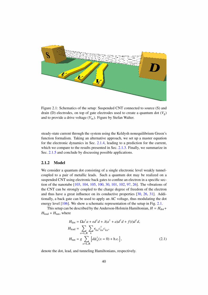
Figure 2.1: Schematics of the setup: Suspended CNT connected to source (S) anddrain (D) electrodes, on top of gate electrodes used to create a quantum dot (Vg)and to provide a drive voltage (Vac). Figure by Stefan Walter.
steady-state current through the system using the Keldysh nonequilibrium Green’sfunction formalism. Taking an alternative approach, we set up a master equationfor the electronic dynamics in Sec. 2.1.4, leading to a prediction for the current,which we compare to the results presented in Sec. 2.1.3. Finally, we summarize inSec. 2.1.5 and conclude by discussing possible applications.
2.1.2 Model
We consider a quantum dot consisting of a single electronic level weakly tunnel-coupled to a pair of metallic leads. Such a quantum dot may be realized on asuspended CNT using electronic back gates to confine an electron in a specific sec-tion of the nanotube [103, 104, 105, 100, 30, 101, 102, 97, 26]. The vibrations ofthe CNT can be strongly coupled to the charge degree of freedom of the electronand thus have a great influence on its conductive properties [30, 26, 31]. Addi-tionally, a back gate can be used to apply an AC voltage, thus modulating the dotenergy level [106]. We show a schematic representation of the setup in Fig. 2.1.
This setup can be described by the Anderson-Holstein Hamiltonian, H = Hdot+
Hlead + Htun, where
Hdot = Ωa†a + εd†d + λ(a† + a)d†d + f (t)d†d,
Hlead =∑α=L,R
∑k
εkαc†kαckα,
Htun = g∑α=L,R
[dψ†α(x = 0) + h.c.
], (2.1)
denote the dot, lead, and tunneling Hamiltonians, respectively.
40
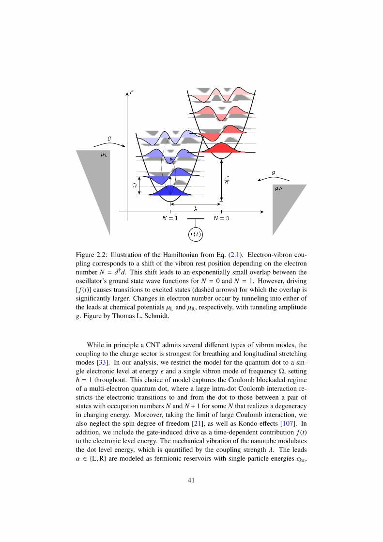
E
N = 1 N = 0
2
f (t)
L
g
R
g
Figure 2.2: Illustration of the Hamiltonian from Eq. (2.1). Electron-vibron cou-pling corresponds to a shift of the vibron rest position depending on the electronnumber N = d†d. This shift leads to an exponentially small overlap between theoscillator’s ground state wave functions for N = 0 and N = 1. However, driving[ f (t)] causes transitions to excited states (dashed arrows) for which the overlap issignificantly larger. Changes in electron number occur by tunneling into either ofthe leads at chemical potentials µL and µR, respectively, with tunneling amplitudeg. Figure by Thomas L. Schmidt.
While in principle a CNT admits several different types of vibron modes, thecoupling to the charge sector is strongest for breathing and longitudinal stretchingmodes [33]. In our analysis, we restrict the model for the quantum dot to a sin-gle electronic level at energy ε and a single vibron mode of frequency Ω, setting~ = 1 throughout. This choice of model captures the Coulomb blockaded regimeof a multi-electron quantum dot, where a large intra-dot Coulomb interaction re-stricts the electronic transitions to and from the dot to those between a pair ofstates with occupation numbers N and N + 1 for some N that realizes a degeneracyin charging energy. Moreover, taking the limit of large Coulomb interaction, wealso neglect the spin degree of freedom [21], as well as Kondo effects [107]. Inaddition, we include the gate-induced drive as a time-dependent contribution f (t)to the electronic level energy. The mechanical vibration of the nanotube modulatesthe dot level energy, which is quantified by the coupling strength λ. The leadsα ∈ L,R are modeled as fermionic reservoirs with single-particle energies εkα,
41
described by fermionic operators ckα obeying the canonical anticommutation rela-tions ckα, c
†
k′β = δkk′δαβ. Finally, Htun describes local electron tunneling into andout of the leads using the Fourier transform ψα(x) = L−1/2 ∑
k eikxck,α, where L isthe length of the lead. An illustration of the Hamiltonian is shown in Fig. 2.2.
In the absence of electron-vibron coupling, the dot features a single resonanceat energy ε. Electron-vibron coupling leads to the emergence of side-peaks at en-ergies ε + nΩ with n ∈ Z. In the following, we focus on the limit of sequentialtunneling. This is the dominant transport process for small g and potential differ-ences eV = µL − µR, where µα is the chemical potential of lead α, such that only asingle resonance lies within the bias window.
The electron-vibron coupling term can be removed by applying the polarontransformation [108] given byU = exp[λ(a† − a)d†d/Ω], leading to
UHU−1 = Ωa†a + εd†d + f (t)d†d
+∑α=L,R
∑k
εkαc†kαckα + g∑α=L,R
[X†dψ†α(x = 0) + h.c.
], (2.2)
where the electron level energy ε is renormalized to ε = ε − λ2/Ω and the electron-vibron coupling is moved to an exponential factor multiplying the tunneling term,X = e−λ(a†−a)/Ω. This leaves us with an expression consisting of a quadratic Hamil-tonian H0 and a weak perturbation H1,
H0 = Ωa†a + εd†d + f (t)d†d +∑α
∑k
εkαc†kαckα
HI = g∑α
[X†dψ†α(x = 0) + h.c.
], (2.3)
which lends itself to a variety of approaches that are perturbative in the tunnelingamplitude g, but still permit potentially large values of the electron-vibron couplingλ Ω.
A great deal of insight into similar models has already been obtained. Specifi-cally, the undriven [ f (t) = 0] variant of the system has been examined with regardto its transport properties [20, 21, 23, 109, 34, 110]. The most striking finding inthis context is that of Franck-Condon blockade: strong electron-vibron interactionleads to formation of a composite state, called a polaron, which can be thoughtof as being made up of an electron and a “cloud” of vibrational excitations sur-rounding it. If the electron is to tunnel out of the quantum dot, this state has to bebroken up, at an energy cost which strongly increases with the coupling, leading toan exponential suppression of tunneling.
In the following, we will investigate in detail the novel effects that arise byperiodically modulating the electronic level energy. We will first show that due tothe strong electron-vibron coupling, this type of drive can be mapped to a driveof the vibron. Moreover, we will demonstrate that it has a strong influence onelectronic transport and that, in particular, the Franck-Condon blockade can be
42
lifted. It is worth pointing out that a small AC drive voltage applied to the gate canlead to an exponentially strong change of the average current.
The physical interpretation of this process is as follows. Due to the electron-vibron coupling, a time-dependent gate voltage also has the effect of driving thevibron, so the vibron will populate an excited state. Importantly, the overlap inte-gral between excited vibron states for different fermion numbers contains Franck-Condon factors which are exponentially larger than those of the vibron groundstates. This makes it possible to lift the Franck-Condon blockade, and hence in-creases the average current.
Hence, the relative change in average current I(A)/I(0), where A is the ampli-tude of the AC gate voltage, is close to an exponential function of A. This makesthe I − V characteristic reminiscent of that of a transistor, albeit now for AC gatevoltages: in our system, a DC bias current can be controlled by a small AC gatevoltage. Note that the frequency of the AC gate voltage needs to be close to thevibron frequency, since the effect relies on the excitation of vibrons.
2.1.3 Polaron tunneling approximation
In the following, we use a Keldysh Green’s function approach to analyze the in-fluence of the gate voltage on the conductance of the system. The most importantmeasurable quantity in this context is the steady-state current 〈I〉ss. In the follow-ing, we work with the current through the right lead, noting that it is identical tothe one through the left lead up to a displacement current introduced by the timedependence of the drive. However, since this current oscillates on a timescale givenby the inverse drive frequency, much faster than the tunneling rates to and from thedot, we can safely neglect it on average. Thus 〈I〉ss is obtained from expectationvalue of the operator
IR(t) = eddt
∑k
c†kRckR = −ie
∑k
c†kRckR,H
= ieg
[d†(t)X(t)ψR(t) − ψ†R(t)X†(t)d(t)
], (2.4)
where e is the negative electron charge. It will prove expedient to move the time de-pendence into the perturbative part of the Hamiltonian, which can be accomplishedby applying the unitary transformation given byV(t) = exp
[id†d
∫ tt0
ds f (s)]. This
reduces the quadratic Hamiltonian to H0 = εd†d + Ωa†a, and changes the polaronoperator to
X(t) ≡ V(t)X(t)V−1(t) = e−λΩ [a†eiΩt−ae−iΩt+iF(t)], (2.5)
with F(t) = Ωλ
∫ tt0
ds f (t) denoting the integrated drive, where the initial time t0 al-ways cancels in the following and can hence be chosen arbitrarily. The transformedcoupling Hamiltonian then reads
HI = g∑α
[X†dψ†α(x = 0) + h.c.
]. (2.6)
43
It bears pointing out that as a result of the transformation V the drive has thusbeen moved onto the vibrational part of the Hamiltonian, lending substance to theintuition that the coupling between electrons and vibrons leads to the possibility ofdriving the vibrons by driving the electrons.
In the following, we focus on a resonant harmonic drive, f (t) = A cos(Ωt). Aslaid out in Sec. 1.2.3, the Keldysh Green’s function formalism together with pertur-bation theory in the lead coupling g can be employed to calculate the mean steady-state current [48] from the retarded dot Green’s function DR for the undriven case,
〈I〉 = ieΓ
2
∫dω2π
[nFL(ω) − nFR(ω)][DR(ω) − DA(ω)
], (2.7)
where the coupling g and the lead density of states ρ are absorbed into the tun-neling rate Γ = 2πρg2. We use the wide-band approximation, so the density ofstates is constant, ρ = 1/(2πvF) with Fermi velocity vF. In this section, Eq. (2.7)will be used as an approximation to the current in the presence of drive. A moreexact treatment using the Floquet formalism is presented in Sec. 2.2. To obtain theaverage current, we thus need to calculate the nonequilibrium dot Green’s function
D(τ, τ′) = −i⟨TCd†(τ)X(τ)X†(τ′)d(τ′)e−i
∫C dσHI(σ)
⟩0, (2.8)
with components Di j(t, t′), where the indices i, j = +,− denote the forward andbackward branches of the Keldysh contour C from Fig. 1.3, with the initial timelying in the infinite past. Comparing with the notation of Sec. 2.2, it should bealso noted that D(τ, t′) as used here contains both electronic and vibrational oper-ators. The expectation value in Eq. (2.8) is taken with respect to the HamiltonianH0 of the non-interacting system, and the time dependences are understood to bein the interaction picture corresponding to H0. We note that the presence of the vi-brational operators X in this expression is a consequence of the polaron transformdressing the electron. As the non-interacting Hamiltonian is not quadratic in X, X†,Wick’s theorem does not hold for these operators, so the calculation of the termsmaking up the Green’s function in Eq. (2.8) seems rather daunting.
Drawing upon Ref. [35], we hence employ the following approximation: thedwell time of the electron on the quantum dot (which can be estimated as the in-verse of the bare tunneling rate Γ) is large compared to the timescale of the polaronwhich is associated with the inverse of the energy shift ε − ε = λ2/Ω. In this limit,the polaron will relax in the time between two tunneling processes. The diagram-matic form of this polaron-tunneling approximation (PTA) is given in Fig. 2.3,and it has been used before to calculate transport properties of strongly coupledelectron-vibron systems. [35, 111, 112] The purpose of this approximation is toavoid having to explicitly expand the exponential from Eq. (2.8) in powers of thetunneling amplitude g. Instead, the 2n-th order vibrational correction to the baredot Green’s function Gdot(τ − τ′) = −i〈TCd(τ)d†(τ′)〉 is seen to be caused by a se-ries of tunneling processes to and from the leads, where the lead Green’s function
44
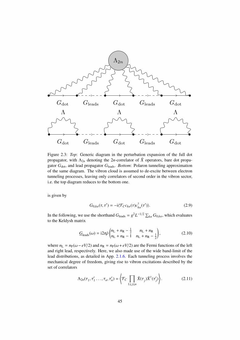
Λ2n
Gdot Gleads Gdot Gleads Gdot
Gdot Gleads Gdot Gleads Gdot
Λ Λ Λ
Figure 2.3: Top: Generic diagram in the perturbation expansion of the full dotpropagator, with Λ2n denoting the 2n-correlator of X operators, bare dot propa-gator Gdot, and lead propagator Gleads. Bottom: Polaron tunneling approximationof the same diagram. The vibron cloud is assumed to de-excite between electrontunneling processes, leaving only correlators of second order in the vibron sector,i.e. the top diagram reduces to the bottom one.
is given by
G0,kα(τ, τ′) = −i〈TCckα(τ)c†kα(τ′)〉. (2.9)
In the following, we use the shorthand Gleads = g2L−1/2 ∑kα G0,kα, which evaluates
to the Keldysh matrix
Gleads(ω) = i2πρ(nL + nR −
12 nL + nR
nL + nR − 1 nL + nR −12
), (2.10)
where nL = nF(ω− eV/2) and nR = nF(ω+ eV/2) are the Fermi functions of the leftand right lead, respectively. Here, we also made use of the wide band-limit of thelead distributions, as detailed in App. 2.1.6. Each tunneling process involves themechanical degree of freedom, giving rise to vibron excitations described by theset of correlators
Λ2n(τ1, τ′1 . . . , τn, τ
′n) =
⟨TC
∏1≤ j≤n
X(τ j)X†(τ′j)
⟩. (2.11)
45
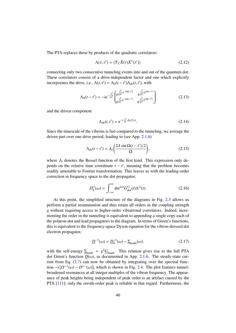
The PTA replaces these by products of the quadratic correlators
Λ(τ, τ′) = 〈TC X(τ)X†(τ′)〉 (2.12)
connecting only two consecutive tunneling events into and out of the quantum dot.These correlators consist of a drive-independent factor and one which explicitlyincorporates the drive, i.e., Λ(t, t′) = Λ0(t − t′)Λdr(t, t′), with
Λ0(t − t′) = −ie−λ2
Ω2
eλ2
Ω2 e−iΩ|t−t′ |eλ2
Ω2 eiΩ(t−t′)
eλ2
Ω2 e−iΩ(t−t′)eλ2
Ω2 eiΩ|t−t′ |,
(2.13)
and the driven component
Λdr(t, t′) = e−i∫ t
t′ ds f (s). (2.14)
Since the timescale of the vibrons is fast compared to the tunneling, we average thedriven part over one drive period, leading to (see App. 2.1.6)
Λdr(t − t′) = J0
(2A sin Ω(t − t′)/2
Ω
), (2.15)
where J0 denotes the Bessel function of the first kind. This expression only de-pends on the relative time coordinate t − t′, meaning that the problem becomesreadily amenable to Fourier transformation. This leaves us with the leading-ordercorrection in frequency space to the dot propagator,
Di j0 (ω) =
∫ ∞
−∞
dteiωtGi jdot(t)Λ
i j(t). (2.16)
At this point, the simplified structure of the diagrams in Fig. 2.3 allows usperform a partial resummation and thus retain all orders in the coupling strengthg without requiring access to higher-order vibrational correlators. Indeed, incre-menting the order in the tunneling is equivalent to appending a single copy each ofthe polaron-dot and lead propagators to the diagram. In terms of Green’s functions,this is equivalent to the frequency-space Dyson equation for the vibron-dressed dotelectron propagator,
D−1(ω) = D−10 (ω) − Σleads(ω). (2.17)
with the self-energy Σleads = g2Gleads. This relation gives rise to the full PTAdot Green’s function D(ω), as documented in App. 2.1.6. The steady-state cur-rent from Eq. (2.7) can now be obtained by integrating over the spectral func-tion −i
[D−+(ω) − D+−(ω)
], which is shown in Fig. 2.4. The plot features tunnel-
broadened resonances at all integer multiples of the vibron frequency. The appear-ance of peak heights being independent of peak order is an artifact caused by thePTA [111]; only the zeroth-order peak is reliable in that regard. Furthermore, the
46
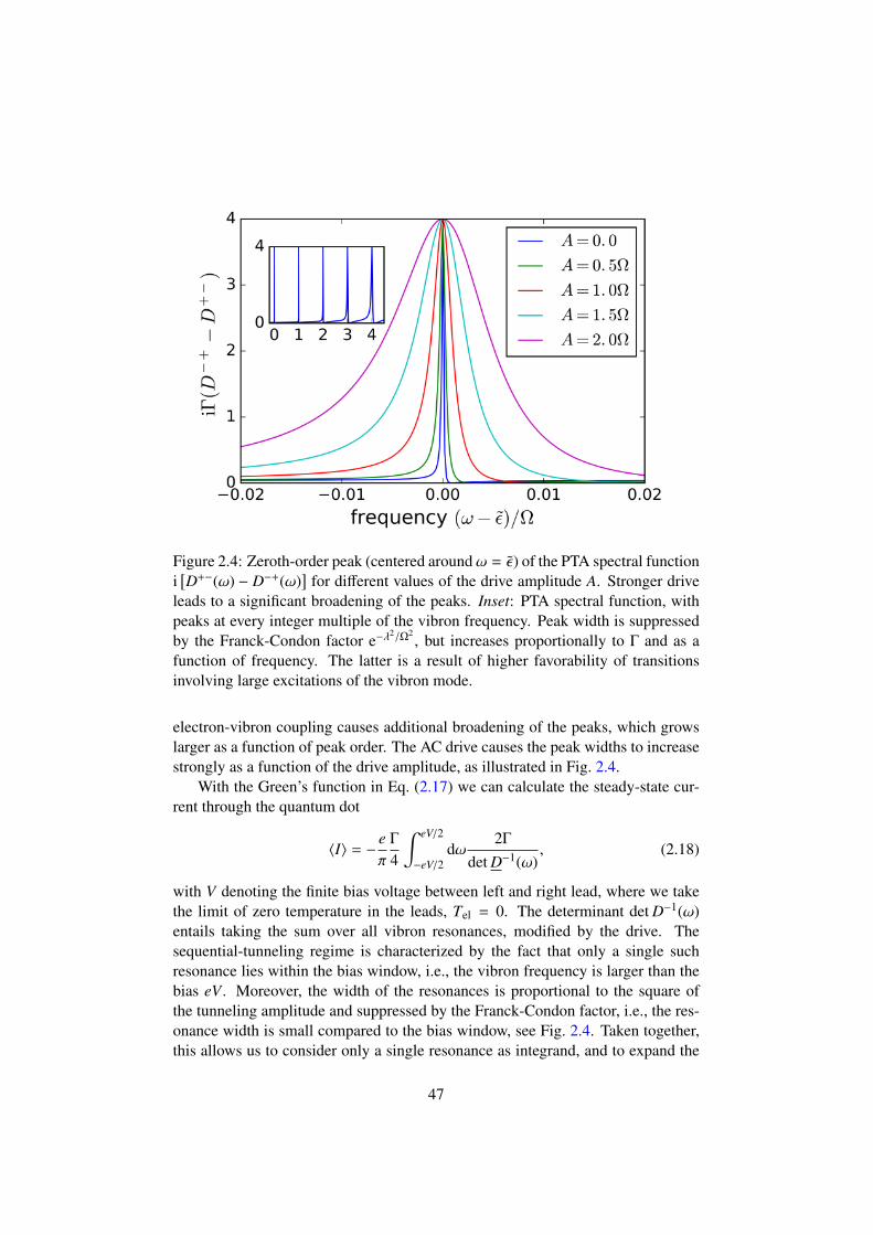
Figure 2.4: Zeroth-order peak (centered aroundω = ε) of the PTA spectral functioni[D+−(ω) − D−+(ω)
]for different values of the drive amplitude A. Stronger drive
leads to a significant broadening of the peaks. Inset: PTA spectral function, withpeaks at every integer multiple of the vibron frequency. Peak width is suppressedby the Franck-Condon factor e−λ
2/Ω2, but increases proportionally to Γ and as a
function of frequency. The latter is a result of higher favorability of transitionsinvolving large excitations of the vibron mode.
electron-vibron coupling causes additional broadening of the peaks, which growslarger as a function of peak order. The AC drive causes the peak widths to increasestrongly as a function of the drive amplitude, as illustrated in Fig. 2.4.
With the Green’s function in Eq. (2.17) we can calculate the steady-state cur-rent through the quantum dot
〈I〉 = −eπ
Γ
4
∫ eV/2
−eV/2dω
2Γ
det D−1(ω), (2.18)
with V denoting the finite bias voltage between left and right lead, where we takethe limit of zero temperature in the leads, Tel = 0. The determinant det D−1(ω)entails taking the sum over all vibron resonances, modified by the drive. Thesequential-tunneling regime is characterized by the fact that only a single suchresonance lies within the bias window, i.e., the vibron frequency is larger than thebias eV . Moreover, the width of the resonances is proportional to the square ofthe tunneling amplitude and suppressed by the Franck-Condon factor, i.e., the res-onance width is small compared to the bias window, see Fig. 2.4. Taken together,this allows us to consider only a single resonance as integrand, and to expand the
47
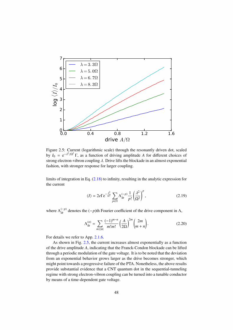
0.0 0.4 0.8 1.2 1.6
drive A/Ω
0
1
2
3
4
5
6
7lo
g ⟨ I⟩ /
I 0
λ= 3. 3Ω
λ= 5. 0Ω
λ= 6. 7Ω
λ= 8. 3Ω
Figure 2.5: Current (logarithmic scale) through the resonantly driven dot, scaledby I0 = e−λ
2/Ω2Γ, as a function of driving amplitude A for different choices of
strong electron-vibron coupling λ. Drive lifts the blockade in an almost exponentialfashion, with stronger response for larger coupling.
limits of integration in Eq. (2.18) to infinity, resulting in the analytic expression forthe current
〈I〉 = 2eΓe−λ2
Ω2∑p∈N
Λ(−p)dr
1p!
(λ2
Ω2
)p
, (2.19)
where Λ(−p)dr denotes the (−p)th Fourier coefficient of the drive component in Λ,
Λ(n)dr =
∑m≥|n|
(−1)m−n
m!m!
( A2Ω
)2m (2m
m + n
). (2.20)
For details we refer to App. 2.1.6.As shown in Fig. 2.5, the current increases almost exponentially as a function
of the drive amplitude A, indicating that the Franck-Condon blockade can be liftedthrough a periodic modulation of the gate voltage. It is to be noted that the deviationfrom an exponential behavior grows larger as the drive becomes stronger, whichmight point towards a progressive failure of the PTA. Nonetheless, the above resultsprovide substantial evidence that a CNT quantum dot in the sequential-tunnelingregime with strong electron-vibron coupling can be turned into a tunable conductorby means of a time-dependent gate voltage.
48
2.1.4 Born-Markov analysis
In this section we make use of an alternative approach to the setup under con-sideration, thus supplementing the result of the Green’s function calculation. Inparticular, we aim to obtain an estimate of the validity the PTA, whose compati-bility with a time-dependent drive of the electronic level energy is still untested.For the purposes of the following discussion, it suffices to take into account a sin-gle lead, and instead of a steady-state current, study the tunneling rates into thislead, which in the limit of sequential tunneling is proportional to the conductance.[23] The comparability of the latter two quantities is a feature of the sequential-tunneling regime, where the current is made up of consecutive, non-overlappingsingle-electron tunneling transitions.
The system being weakly coupled to a metallic lead with intractably manydegrees of freedom motivates us to perform a partial trace over these lead degreesof freedom. This is the open systems approach outlined in Sec. 1.4: We treat thequantum dot as an open quantum system and the lead as an electron reservoir.[113] The weak coupling Hamiltonian HI then takes the role of the perturbativesystem-bath interaction. Under the Born-Markov approximation, the evolution ofthe system density matrix ρS(t) is governed by the quantum master equation [57]
ddtρS(t) = −
∫ ∞
0ds trB[HI(t), [HI(t − s), ρS(t) ⊗ ρB]], (2.21)
where the time-dependence in the interaction picture (denoted by a hat) is under-stood with respect to the quadratic Hamiltonian Ωa†a + [ε + f (t)]d†d, and ρB de-notes the bath density matrix. At this point, an additional simplification presentsitself as a consequence of the configuration of our quantum dot: in the Coulombblockade and sequential tunneling regimes not only the lead excitations, but alsothe vibrations have fast dynamics compared to the electron on the quantum dot.This means that after the polaron transform the non-perturbative part of the Hamil-tonian no longer couples the charge and vibrational degrees of freedom. Hencewe can extend the bath to also include the vibron, leaving only the electron in thesystem. [114, 115] This leads to the bath density matrix composed of the vibronsand the lead ρB = ρvib ⊗ ρlead. Note that the separation of time scales betweenelectron and vibron relaxation is similar to the reasoning used to motivate the PTAin the previous section. Nevertheless, the two approximations correspond to dif-ferent partial resummations of a perturbation series and should not be expected tocoincide quantitatively.
As outlined in Sec. 1.4, the Born-Markov master equation can be cast in Lind-blad form, meaning that a set of coefficients hµ and system operators Cµ can befound with
ddtρS =
∑µ
hµ
(CµρSC†µ −
12
ρS, C†µCµ
). (2.22)
49

Since in our case the vibron degree of freedom is traced over, the Lindblad opera-tors Cµ will be simple functions of the electronic creation and annihilation opera-tors.
However, the presence of the driving term f (t)d†d casts doubts upon the va-lidity of the approximations leading to this form: in particular, driving the systemwith a frequency comparable to Ω, as is realistic in the CNT setup, is in conflictwith the assumption of separation of time scales, now that the bath includes thevibron. Therefore, we propose the following alternative path to incorporate driv-ing: in a fashion reminiscent of the transformation V from the previous section,the driving term can be moved onto the vibron sector, where it then can be takeninto account by modifying the vibron density matrix in the master equation (2.21).Assuming equilibrium Fermi distributions nF(ω) in the lead, the master equationthen reads
ddtρS(t) = −g2
∫ ∞
0ds
∫dω[⟨
X(t)X†(t − s)⟩
nF(ω)dd†ei(−ε+ω)sρS(t)
+⟨X†(t)X(t − s)
⟩(1 − nF(ω)) d†de−i(−ε+ω)sρS(t)
−⟨X†(t − s)X(t)
⟩dρS(t)d† (1 − nF (ω)) ei(−ε+ω)s
−⟨X(t − s)X†(t)
⟩d†ρS(t)dnF(ω)e−i(−ε+ω)s
]+ h.c. (2.23)
where the expectation values are taken with respect to the vibron density matrixρvib, which we use below to take into account the drive. Moreover, X(t) = exp
[−
λΩ
(a†eiΩt − ae−iΩt
) ]denotes the exponential vibron operator. We again assume the
lead to be at zero temperature, Tel = 0. In the following, we explore differentchoices for ρvib, and study the resulting electron tunneling rates.
Vibron in the ground state
To begin with, we assume an unoccupied vibron state and thus ρ(0)vib = |0〉 〈0|, cor-
responding to the absence of driving and zero temperature. In this case, the tracesin Eq. (2.23) are readily performed. Comparing to the master equation in Lind-blad form Eq. (2.22) leads to the Lindblad operators C(0)
in = d† and C(0)out = d with
coefficients
h(0)in =
Γ
2e−
λ2
Ω2∑n≥0
(λ2/Ω2
)n
n!nF(ε + nΩ),
h(0)out =
Γ
2e−
λ2
Ω2∑n≥0
(λ2/Ω2
)n
n!(1 − nF(ε − nΩ)) , (2.24)
where Γ is defined as before. Due to the specific form of the Lindblad operators,the coefficients h(0)
in and h(0)out are proportional to the electron tunneling rates. Specif-
ically, the respective appearances of nF and 1−nF indicate that h(0)out governs the case
50
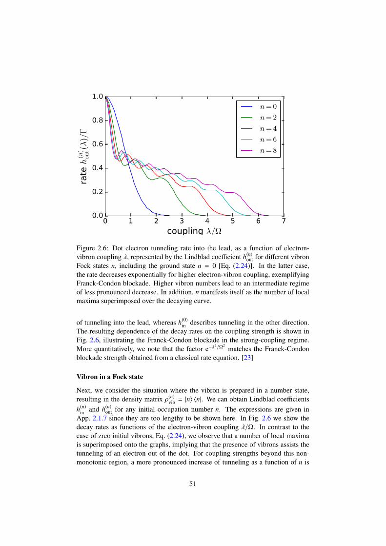
0 1 2 3 4 5 6 7
coupling λ/Ω
0.0
0.2
0.4
0.6
0.8
1.0
rate
h(n
)ou
t(λ
)/Γ
n= 0
n= 2
n= 4
n= 6
n= 8
Figure 2.6: Dot electron tunneling rate into the lead, as a function of electron-vibron coupling λ, represented by the Lindblad coefficient h(n)
out for different vibronFock states n, including the ground state n = 0 [Eq. (2.24)]. In the latter case,the rate decreases exponentially for higher electron-vibron coupling, exemplifyingFranck-Condon blockade. Higher vibron numbers lead to an intermediate regimeof less pronounced decrease. In addition, n manifests itself as the number of localmaxima superimposed over the decaying curve.
of tunneling into the lead, whereas h(0)in describes tunneling in the other direction.
The resulting dependence of the decay rates on the coupling strength is shown inFig. 2.6, illustrating the Franck-Condon blockade in the strong-coupling regime.More quantitatively, we note that the factor e−λ
2/Ω2matches the Franck-Condon
blockade strength obtained from a classical rate equation. [23]
Vibron in a Fock state
Next, we consider the situation where the vibron is prepared in a number state,resulting in the density matrix ρ(n)
vib = |n〉 〈n|. We can obtain Lindblad coefficientsh(n)
in and h(n)out for any initial occupation number n. The expressions are given in
App. 2.1.7 since they are too lengthy to be shown here. In Fig. 2.6 we show thedecay rates as functions of the electron-vibron coupling λ/Ω. In contrast to thecase of zreo initial vibrons, Eq. (2.24), we observe that a number of local maximais superimposed onto the graphs, implying that the presence of vibrons assists thetunneling of an electron out of the dot. For coupling strengths beyond this non-monotonic region, a more pronounced increase of tunneling as a function of n is
51
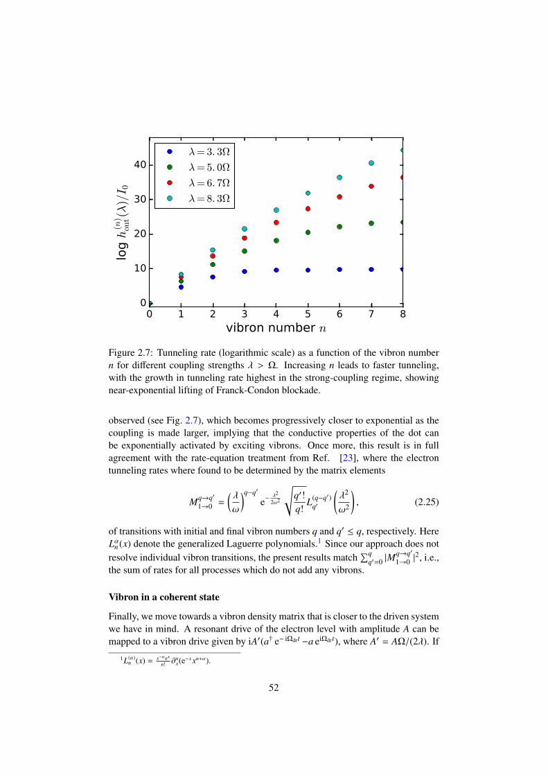
0 1 2 3 4 5 6 7 8
vibron number n
0
10
20
30
40
log h
(n)
out(λ
)/I 0
λ= 3. 3Ω
λ= 5. 0Ω
λ= 6. 7Ω
λ= 8. 3Ω
Figure 2.7: Tunneling rate (logarithmic scale) as a function of the vibron numbern for different coupling strengths λ > Ω. Increasing n leads to faster tunneling,with the growth in tunneling rate highest in the strong-coupling regime, showingnear-exponential lifting of Franck-Condon blockade.
observed (see Fig. 2.7), which becomes progressively closer to exponential as thecoupling is made larger, implying that the conductive properties of the dot canbe exponentially activated by exciting vibrons. Once more, this result is in fullagreement with the rate-equation treatment from Ref. [23], where the electrontunneling rates where found to be determined by the matrix elements
Mq→q′
1→0 =
(λ
ω
)q−q′
e−λ2
2ω2
√q′!q!
L(q−q′)q′
(λ2
ω2
), (2.25)
of transitions with initial and final vibron numbers q and q′ ≤ q, respectively. HereLαn (x) denote the generalized Laguerre polynomials.1 Since our approach does notresolve individual vibron transitions, the present results match
∑qq′=0 |M
q→q′
1→0 |2, i.e.,
the sum of rates for all processes which do not add any vibrons.
Vibron in a coherent state
Finally, we move towards a vibron density matrix that is closer to the driven systemwe have in mind. A resonant drive of the electron level with amplitude A can bemapped to a vibron drive given by iA′(a† e− iΩdrt −a eiΩdrt), where A′ = AΩ/(2λ). If
1L(α)n (x) = x−αex
n! ∂nx(e−x xn+α).
52
we in addition introduce a vibron damping rate γ to prevent divergences that mightarise from driving a part of the bath, this generates the coherent vibron state [116]|δ〉 with δ ∝ iA′/(Ωdr − Ω + iγ). Therefore, we consider the vibron density matrixρ(δ)
vib = |δ〉 〈δ|. For this case, we obtain the Lindblad coefficients
h(δ)in =
Γ
2e−
λ2
Ω2 e−i2 λΩ
(sin(Ωt) Re δ−cos(Ωt) Im δ)∑
m,l∈Z
ei(m+l)Ωt∑n≥0
×
(λ2/Ω2
)n
n!ilJm
(2λ
ΩRe δ
)Jl
(−2
λ
ΩIm δ
)nF(ε + (m + l + n)Ω),
h(δ)out =
Γ
2e−
λ2
Ω2 e−i2 λΩ
(sin(Ωt) Re δ−cos(Ωt) Im δ)∑
m,l∈Z
ei(m+l)Ωt∑n≥0
×
(λ2/Ω2
)n
n!ilJm
(2λ
ΩRe δ
)Jl
(−2
λ
ΩIm δ
)(1 − nF(ε + (m + l − n)Ω)) , (2.26)
where Jn denotes the nth Bessel function of the first kind. Most strikingly, thesetunneling rates are time dependent, reflecting the fact that coherent states are noteigenstates of the quadratic Hamiltonian H0. The influence of the drive on the de-cay rates can now be examined by varying the coherent state parameter δ. Specif-ically, the coherent state displacement δ is proportional to the drive amplitude A′,meaning it can be used as a measure of drive strength. Moreover, the squared ab-solute value |δ|2 is proportional to the average number of vibrons in the coherentstate, which establishes a link to the Fock state situation discussed previously.
In case of resonant driving, the real part Re δ dominates and its magnitude isdirectly proportional to the drive amplitude. However, the off-resonant situationcan be studied in the same fashion by allowing for an imaginary part in δ. Thereit turns out that detuning between drive and vibron mode reduces the electron tun-neling rate, which is in line with the intuition that the conductance is primarilyaffected by the number of vibrons present on the dot.
In order to make a comparison to the results obtained previously, we proceed toexamine the average of h(δ)
out over one drive period, which can be seen as analogousto the averaging performed to obtain Eq. (2.13) in Sec. 2.1.3. The outcome of thisprocedure is shown in Fig. 2.8.
Comparing the rates for different values of the drive amplitude uncovers threedifferent regimes: (i) a weak-coupling regime, where increasing the driving strengthdecreases the tunneling rates, (ii) an intermediate regime showing a moderate in-crease of the tunneling rates for an increased drive, and (iii) a strong-couplingregime which features an almost exponential rise in tunneling rates as the drivingstrength is increased. The weak-coupling behavior is mainly an electronic effect:the favored tunneling transition here is the one that does not involve any vibrations.If the drive amplitude is less than the energy gap between dot and lead, there is lit-tle effect, but if it is significantly larger, the dot will spend a sizable part of thedrive period below the lead; in this position, tunneling is energetically suppressed.For larger drive amplitudes, the portion of a drive period spent below the lead ap-
53
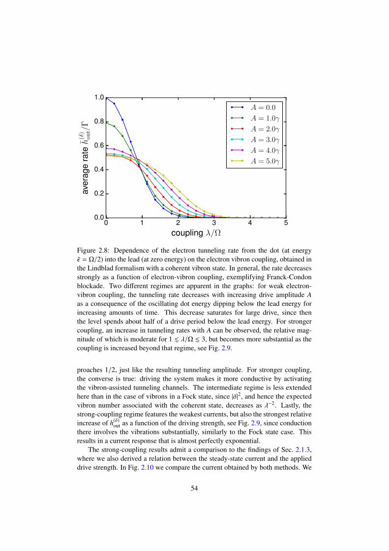
0 1 2 3 4 5coupling λ/Ω
0.0
0.2
0.4
0.6
0.8
1.0
aver
age
rateh
(δ)
out/
Γ
A = 0.0
A = 1.0γ
A = 2.0γ
A = 3.0γ
A = 4.0γ
A = 5.0γ
Figure 2.8: Dependence of the electron tunneling rate from the dot (at energyε = Ω/2) into the lead (at zero energy) on the electron vibron coupling, obtained inthe Lindblad formalism with a coherent vibron state. In general, the rate decreasesstrongly as a function of electron-vibron coupling, exemplifying Franck-Condonblockade. Two different regimes are apparent in the graphs: for weak electron-vibron coupling, the tunneling rate decreases with increasing drive amplitude Aas a consequence of the oscillating dot energy dipping below the lead energy forincreasing amounts of time. This decrease saturates for large drive, since thenthe level spends about half of a drive period below the lead energy. For strongercoupling, an increase in tunneling rates with A can be observed, the relative mag-nitude of which is moderate for 1 . λ/Ω . 3, but becomes more substantial as thecoupling is increased beyond that regime, see Fig. 2.9.
proaches 1/2, just like the resulting tunneling amplitude. For stronger coupling,the converse is true: driving the system makes it more conductive by activatingthe vibron-assisted tunneling channels. The intermediate regime is less extendedhere than in the case of vibrons in a Fock state, since |δ|2, and hence the expectedvibron number associated with the coherent state, decreases as λ−2. Lastly, thestrong-coupling regime features the weakest currents, but also the strongest relativeincrease of h(δ)
out as a function of the driving strength, see Fig. 2.9, since conductionthere involves the vibrations substantially, similarly to the Fock state case. Thisresults in a current response that is almost perfectly exponential.
The strong-coupling results admit a comparison to the findings of Sec. 2.1.3,where we also derived a relation between the steady-state current and the applieddrive strength. In Fig. 2.10 we compare the current obtained by both methods. We
54
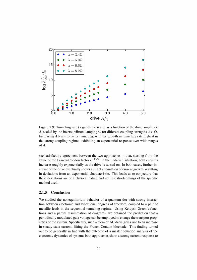
0.0 1.0 2.0 3.0 4.0 5.0drive A/γ
0
5
10
15
20lo
gh
(δ)
out/I 0
λ = 3.4Ω
λ = 5.0Ω
λ = 6.6Ω
λ = 8.2Ω
Figure 2.9: Tunneling rate (logarithmic scale) as a function of the drive amplitudeA, scaled by the inverse vibron damping γ, for different coupling strengths λ > Ω.Increasing A leads to faster tunneling, with the growth in tunneling rate highest inthe strong-coupling regime, exhibiting an exponential response over wide rangesof A.
see satisfactory agreement between the two approaches in that, starting from thevalue of the Franck-Condon factor e−λ
2/Ω2in the undriven situation, both currents
increase roughly exponentially as the drive is turned on. In both cases, further in-crease of the drive eventually shows a slight attenuation of current growth, resultingin deviations from an exponential characteristic. This leads us to conjecture thatthese deviations are of a physical nature and not just shortcomings of the specificmethod used.
2.1.5 Conclusion
We studied the nonequilibrium behavior of a quantum dot with strong interac-tion between electronic and vibrational degrees of freedom, coupled to a pair ofmetallic leads in the sequential-tunneling regime. Using Keldysh Green’s func-tions and a partial resummation of diagrams, we obtained the prediction that aperiodically modulated gate voltage can be employed to change the transport prop-erties of the system. Specifically, such a form of AC drive gives rise to an increasein steady-state current, lifting the Franck-Condon blockade. This finding turnedout to be generally in line with the outcome of a master equation analysis of theelectronic dynamics of system: both approaches show a strong current response to
55
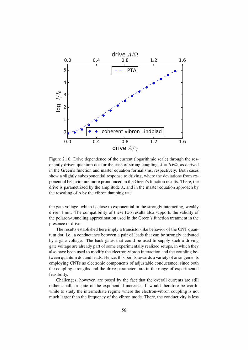
0.0 0.4 0.8 1.2 1.6
drive A/γ
0
1
2
3
4
5
log I/I 0
coherent vibron Lindblad
0.0 0.4 0.8 1.2 1.6drive A/Ω
PTA
Figure 2.10: Drive dependence of the current (logarithmic scale) through the res-onantly driven quantum dot for the case of strong coupling, λ = 6.6Ω, as derivedin the Green’s function and master equation formalisms, respectively. Both casesshow a slightly subexponential response to driving, where the deviations from ex-ponential behavior are more pronounced in the Green’s function results. There, thedrive is parametrized by the amplitude A, and in the master equation approach bythe rescaling of A by the vibron damping rate.
the gate voltage, which is close to exponential in the strongly interacting, weaklydriven limit. The compatibility of these two results also supports the validity ofthe polaron-tunneling approximation used in the Green’s function treatment in thepresence of drive.
The results established here imply a transistor-like behavior of the CNT quan-tum dot, i.e., a conductance between a pair of leads that can be strongly activatedby a gate voltage. The back gates that could be used to supply such a drivinggate voltage are already part of some experimentally realized setups, in which theyalso have been used to modify the electron-vibron interaction and the coupling be-tween quantum dot and leads. Hence, this points towards a variety of arrangementsemploying CNTs as electronic components of adjustable conductance, since boththe coupling strengths and the drive parameters are in the range of experimentalfeasibility.
Challenges, however, are posed by the fact that the overall currents are stillrather small, in spite of the exponential increase. It would therefore be worth-while to study the intermediate regime where the electron-vibron coupling is notmuch larger than the frequency of the vibron mode. There, the conductivity is less
56
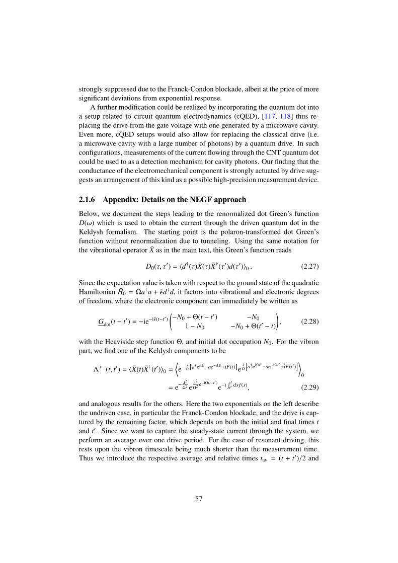
strongly suppressed due to the Franck-Condon blockade, albeit at the price of moresignificant deviations from exponential response.
A further modification could be realized by incorporating the quantum dot intoa setup related to circuit quantum electrodynamics (cQED), [117, 118] thus re-placing the drive from the gate voltage with one generated by a microwave cavity.Even more, cQED setups would also allow for replacing the classical drive (i.e.a microwave cavity with a large number of photons) by a quantum drive. In suchconfigurations, measurements of the current flowing through the CNT quantum dotcould be used to as a detection mechanism for cavity photons. Our finding that theconductance of the electromechanical component is strongly actuated by drive sug-gests an arrangement of this kind as a possible high-precision measurement device.
2.1.6 Appendix: Details on the NEGF approach
Below, we document the steps leading to the renormalized dot Green’s functionD(ω) which is used to obtain the current through the driven quantum dot in theKeldysh formalism. The starting point is the polaron-transformed dot Green’sfunction without renormalization due to tunneling. Using the same notation forthe vibrational operator X as in the main text, this Green’s function reads
D0(τ, τ′) = 〈d†(τ)X(τ)X†(τ′)d(τ′)〉0 . (2.27)
Since the expectation value is taken with respect to the ground state of the quadraticHamiltonian H0 = Ωa†a + εd†d, it factors into vibrational and electronic degreesof freedom, where the electronic component can immediately be written as
Gdot(t − t′) = −ie−iε(t−t′)(−N0 + Θ(t − t′) −N0
1 − N0 −N0 + Θ(t′ − t)
), (2.28)
with the Heaviside step function Θ, and initial dot occupation N0. For the vibronpart, we find one of the Keldysh components to be
Λ+−(t, t′) = 〈X(t)X†(t′)〉0 =
⟨e−
λΩ [a†eiΩt−ae−iΩt+iF(t)]e
λΩ
[a†eiΩt′−ae−iΩt′+iF(t′)
]⟩0
= e−λ2
Ω2 eλ2
Ω2 e−iΩ(t−t′)e−i
∫ tt′ ds f (s), (2.29)
and analogous results for the others. Here the two exponentials on the left describethe undriven case, in particular the Franck-Condon blockade, and the drive is cap-tured by the remaining factor, which depends on both the initial and final times tand t′. Since we want to capture the steady-state current through the system, weperform an average over one drive period. For the case of resonant driving, thisrests upon the vibron timescale being much shorter than the measurement time.Thus we introduce the respective average and relative times tav = (t + t′)/2 and
57
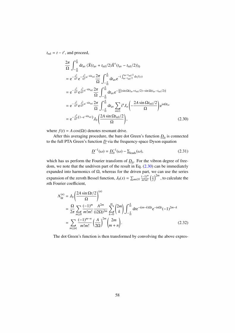
trel = t − t′, and proceed,
2πΩ
∫ πΩ
− πΩ
dtav 〈X(tav + trel/2)X†(tav − trel/2)〉0
= e−λ2
Ω2 e−λ2
Ω2 e−iΩtrel 2πΩ
∫ πΩ
− πΩ
dtave−i∫ tav+trel/2
tav−trel/2ds f (s)
= e−λ2
Ω2 eλ2
Ω2 e−iΩtrel 2πΩ
∫ πΩ
− πΩ
dtave−iAΩ
[sin Ω(tav+trel/2)−sin Ω(tav−trel/2)]
= e−λ2
Ω2 eλ2
Ω2 e−iΩtrel 2πΩ
∫ πΩ
− πΩ
dtav
∑n∈Z
inJn
(−
2A sin Ωtrel/2Ω
)einΩtav
= e−λ2
Ω2 (1−e−iΩtrel)J0
(2A sin Ωtrel/2
Ω
), (2.30)
where f (t) = A cos(Ωt) denotes resonant drive.After this averaging procedure, the bare dot Green’s function D0 is connected
to the full PTA Green’s function D via the frequency-space Dyson equation
D−1(ω) = D−10 (ω) − Σleads(ω), (2.31)
which has us perform the Fourier transform of D0. For the vibron degree of free-dom, we note that the undriven part of the result in Eq. (2.30) can be immediatelyexpanded into harmonics of Ω, whereas for the driven part, we can use the seriesexpansion of the zeroth Bessel function, J0(x) =
∑m∈N
(−1)m
m!m!
(x2
)2m, to calculate the
nth Fourier coefficient,
Λ(n)dr = J0
(2A sin Ωt/2
Ω
)(n)
=Ω
2π
∑m≥0
(−1)m
m!m!A2m
(i2Ω)2m
m∑k=0
(2mk
) ∫ πΩ
− πΩ
dte−i(m−k)Ωte−inΩt(−1)2m−k
=∑m≥|n|
(−1)m−n
m!m!
( A2Ω
)2m (2m
m + n
). (2.32)
The dot Green’s function is then transformed by convolving the above expres-
58
sion with the undriven vibron and bare electron parts,
D0(ω) = F
[−ie−iεte−
λ2
Ω2 J0
(2A sin(Ωt/2)
Ω
) Θ(t)eλ2
Ω2 e−iΩ|t|0
0 +Θ(−t)eλ2
Ω2 e−iΩ|t|
(ω)
= −i2πe−λ2
Ω2 F
∑n∈N
Λ(n)dr einΩt
∑k∈N
1k!
(λ2
Ω2
)k
eikΩt(Θ(t) 0
0 Θ(−t)
)](ω − ε)
= −i2πe−λ2
Ω2∑
n,k∈N
Λ(n)dr
1k!
(λ2
Ω2
)k ∫ ∞
0 dtei(kΩ+nΩ+ω−ε)t 0
0∫ 0−∞
dtei(kΩ+nΩ+ω−ε)t
= 2πe−
λ2
Ω2 limη→0
∑n,k∈N
Λ(n)dr
1k!
(λ2
Ω2
)k 1kΩ+nΩ+ω−ε+iη 0
0 − 1kΩ+nΩ+ω−ε−iη
, (2.33)
where F denotes Fourier transform between time and frequency domains, and thecutoff η → 0+ serves to keep the integrals finite. We dropped the delta functionson the off-diagonal of the Fourier-transformed bare dot electron Green’s functionbecause those will not contribute when we invert the matrix in the next step.
Similarly to the bare dot electron Green’s function, the sum over the leadGreen’s functions takes shape as
Gleads(ω)
=1L
∑k
i2πnF(ωk)δ(−ωk + ω) + 1−ωk+ω+iη i2πnF(ωk)δ(−ωk + ω)
i2π(nF(ωk) − 1)δ(−ωk + ω) i2πnF(ωk)δ(−ωk + ω) − 1−ωk+ω−iη
,(2.34)
for each of the two leads, where nF again denotes the lead Fermi distribution. Tak-ing the wide-flat-band limit of the lead distribution, we substitute an energy integralfor the sum over lead modes, 1
L∑
k →∫
dEρ(E) ≈ ρ∫
dE, which renders the inte-gration trivial and leaves us us with
Gleads(ω) = i2πρ(nL + nR −
12 nL + nR
nL + nR − 1 nL + nR −12
), (2.35)
where nL = nF(ω− eV/2) and nR = nF(ω+ eV/2). In the polaron tunneling approx-imation, this Green’s function gives rise to the self-energy Σleads = g2σzGleadsσz,with the third Pauli matrix2
σz =
(1 00 −1
). (2.36)
2This Pauli matrix transformation is required to obtain the sign structure of the self-energy, seeEq. (1.39).
59
Now we are in position to use Eq. (2.31) to calculate the PTA dot Green’sfunction,D(ω) =
(D0(ω)−1 − Σleads(ω)
)−1
=1
det D−1(ω)
−
2πe− λ
2
Ω2 ∑n∈Z,k∈N Λ
(n)dr
1k!
(λ2
Ω2
)k1
kΩ+nΩ+ω−ε
−1
− iΓ(nL + nR −
12
)−iΓ(nL + nR)
−iΓ(nL + nR − 1)
2πe− λ
2
Ω2 ∑n∈Z,k∈N Λ
(n)dr
1k!
(λ2
Ω2
)k1
kΩ+nΩ+ω−ε
−1
− iΓ(nL + nR −
12
)
(2.37)with the determinant of the inverse Green’s function matrix given by
det D−1(ω) = −
2πe−λ2
Ω2∑
n∈Z,k∈N
Λ(n)dr
1k!
(λ2
Ω2
)k 1kΩ + nΩ + ω − ε
−2
−Γ2
4. (2.38)
The sum in this expression runs over all resonances of the vibron mode, whereeach resonance peak is in turn dressed by drive-induced contributions of the otherones. The resonances are Poisson-weighted in the case of no drive (A = 0), and theweakly driven case, where Λ(n) is strongly localized around n = 0, may be seen asa perturbed version of this.
The analysis in the main text is concerned with the drive dependence of D(ω)around the lowest resonance, which is obtained from the above result by takingn = −k.
2.1.7 Appendix: Tunneling rates for Fock vibron state
Here, we provide the Lindblad coefficient for the situation of a vibron prepared ina Fock state, with density matrix ρ(n)
vib = |n〉 〈n|. In order to cast the master equationEq. (2.23) into Lindblad form, we calculate the vibron trace
〈n| X†(t)X(t − s) |n〉 = e−λ2
Ω2∑m≥0
(λ2/Ω2)m
m!
n∑k=0
(nk
)(−2λ2/Ω2)k
k!
×
k∑l=0
(kl
)(−1)k−l
2k−l
k−l∑p=0
(k − l
p
)eiΩs(2p−k+l−m), (2.39)
which gives rise to the Lindblad coefficients
h(n)in =
Γ
2e−
λ2
Ω2∑m≥0
(λ2/Ω2)m
m!
n∑k=0
(nk
)(−2λ2/Ω2)k
k!
×
k∑l=0
(kl
)(−1)k−l
2k−l
k−l∑p=0
(k − l
p
)nF(ε − (2p − k + l − m)Ω),
h(n)out =
Γ
2e−
λ2
Ω2∑m≥0
(λ2/Ω2)m
m!
n∑k=0
(nk
)(−2λ2/Ω2)k
k!
×
k∑l=0
(kl
)(−1)k−l
2k−l
k−l∑p=0
(k − l
p
)(1 − nF(ε − (2p − k + l + m)Ω)) . (2.40)
60

The rates resulting from these coefficients are visualized in Fig. 2.6 of the maintext.
61
2.2 Charge pumping in strongly coupled molecular quan-tum dots
The interaction between electrons and the vibrational degrees of freedom of amolecular quantum dot can lead to an exponential suppression of the conduc-tance, an effect which is commonly termed Franck-Condon blockade. Here, weinvestigate this effect in a quantum dot driven by time-periodic gate voltages andtunneling amplitudes using nonequilibrium Green’s functions and a Floquet ex-pansion. Building on previous results showing that driving can lift the Franck-Condon blockade, we investigate driving protocols which can be used to pumpcharge across the quantum dot. In particular, we show that due to the stronglycoupled nature of the system, the pump current at resonance is an exponentialfunction of the drive strength. This section is based on the article Charge pump-ing in strongly coupled molecular quantum dots, written in collaboration with HanHoe Yap, Jiangbin Gong, and Thomas L. Schmidt, published in Phys. Rev. B 96,195432 (2017).
2.2.1 Introduction
Recent progress in fabrication and measurement techniques has broken new groundin the field of nanoscale physics: Currently realizable systems allow for the ex-perimental examination and manipulation of single quantum states, putting withinreach a wide variety of novel effects [97, 95]. Specifically, the transport proper-ties of such systems are the subject of extensive study, on the quest for pioneeringdesigns of electronic components and circuitry.
One of the core promises of nanoelectronics is to accurately generate and con-trol small amounts of current. In such a context, the paradigm of quantum pump-ing [119, 120, 121] has received considerable attention. Charge pumping signifiesa nonzero time-averaged flow of current through a quantum system as a result ofthe temporal variation of one [122, 123] or several [124, 125, 126] system parame-ters, even in the absence of voltage bias. This effect can be achieved, for instance,in a system between two leads at equal chemical potential, where the system pa-rameters are modulated by an external AC signal. Nanoscale charge pumps havepotential uses as sources of quantized, tunable currents [127, 128].
The current generated by a quantum pump generally depends in a significantfashion on the drive protocol, which can manifest in various ways: For example, ifthe drive period is longer than the time scales inherent in the system, an adiabatictime evolution of the system can be used to obtain rather general results for thecurrent [129, 130, 131]. In contrast, for comparatively fast driving, the situation isless straightforward and the resulting pump current tends to depend strongly on theexcited state spectrum of the system in question, as well as on the specific drivingprotocol that is being employed [132, 133].
Charge pumping has been studied frequently in electronic systems. However,nanoscale physics is not limited to electronics alone. In particular, the interactions
62
between charges and optical or mechanical degrees of freedom open up furtheravenues for exploration [99, 98, 96]. A prototypical nanoelectromechanical system(NEMS) exists for instance in the form of carbon nanotubes (CNT) [103, 25, 24,100, 31, 105]. It has recently become possible to use electronic gates to definea quantum dot on a CNT and to tailor the interaction of electrons and quantizedvibrational modes (“vibrons”) of the nanotube [134, 26, 30].
In particular, the interplay between electronic and mechanical degrees of free-dom in a NEMS can have profound consequences for its conductive properties:The simplest such system – a single vibrational mode interacting with an elec-tronic level – already gives rise to an infinite ladder of composite electromechani-cal states (“polarons”) that can in principle contribute to conduction. In the limit ofstrong electron-vibron coupling, the transitions involving low-lying states of thisladder are exponentially suppressed, leading to a drastic reduction in current, a phe-nomenon called Franck-Condon blockade (FCB) [20, 21, 23]. On the other hand, itwas shown recently that an AC gate voltage in resonance with the vibration can beused to actuate conduction channels that are much less strongly suppressed, whichlifts the Franck-Condon blockade exponentially in the drive amplitude [135]. InRef. [135], it was proposed to observe this effect in a CNT quantum dot, since sucha system exhibits the required strong coupling, and the AC gate voltage could besupplied by the gates used to define the quantum dot [106]. Here, we extend thissetup by using additional gates to also modulate the coupling of the quantum dot tothe lead electrodes. The availability of more than one time-dependent parametersthen allows us to build a bridge towards charge pumping.
Here, we study the current response of a Franck-Condon-blockaded quantumdot to several periodic drives. We consider a model for a quantum dot with interact-ing vibrational and electronic sectors, weakly coupled to a pair of metallic leads.A drive protocol is defined which modulates both the coupling to the leads andthe energy level of the dot. As a result of this drive, we find that charge pumpingthrough the dot can be achieved. Interestingly, we find that for drive frequenciesresonant with the vibron mode, the pump current depends exponentially on thedrive amplitude.
Our work is organized as follows: In Sec. 2.2.2, we lay out the model used todescribe a doubly-driven electromechanical quantum dot. Sec. 2.2.3 contains thederivation of the current through the system, where we use the Keldysh nonequi-librium Green’s function method in conjunction with the polaron tunneling ap-proximation and a Floquet expansion. We apply this method to a specific drivingprotocol in Sec. 2.2.5, leading to a description of charge pumping. In Sec. 2.2.6,we summarize our findings and discuss extensions and ideas for application.
2.2.2 Model
In principle, the electronic interactions on a CNT quantum dot can be very com-plex as different vibron modes may couple to the charges in different electronicorbitals. In the following, we capture the essential physics by using as a min-
63
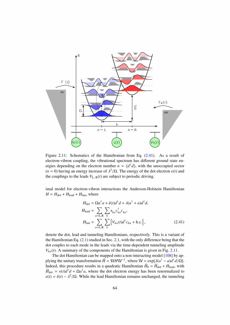
E
n = 1 n = 0
2
(t)VL(t) VR(t)
L
L(t)
R
R(t)
Figure 2.11: Schematics of the Hamiltonian from Eq. (2.41). As a result ofelectron-vibron coupling, the vibrational spectrum has different ground state en-ergies depending on the electron number n =
⟨d†d
⟩, with the unoccupied sector
(n = 0) having an energy increase of λ2/Ω. The energy of the dot electron ε(t) andthe couplings to the leads VL, R(t) are subject to periodic driving.
imal model for electron-vibron interactions the Anderson-Holstein HamiltonianH = Hdot + Hlead + Htun, where
Hdot = Ωa†a + ε(t)d†d + λ(a† + a)d†d,
Hlead =∑α=L,R
∑k
εkαc†kαckα,
Htun =∑α=L,R
∑k
[Vkα(t)d†ckα + h.c.
], (2.41)
denote the dot, lead and tunneling Hamiltonians, respectively. This is a variant ofthe Hamiltonian Eq. (2.1) studied in Sec. 2.1, with the only difference being that thedot couples to each mode in the leads via the time-dependent tunneling amplitudeVkα(t). A summary of the components of the Hamiltonian is given in Fig. 2.11.
The dot Hamiltonian can be mapped onto a non-interacting model [108] by ap-plying the unitary transformation H = UHU−1, whereU = exp[λ(a† − a)d†d/Ω].Indeed, this procedure results in a quadratic Hamiltonian H0 = Hdot + Hlead, withHdot = ε(t)d†d + Ωa†a, where the dot electron energy has been renormalized toε(t) = ε(t) − λ2/Ω. While the lead Hamiltonian remains unchanged, the tunneling
64
amplitudes are dressed by an exponential vibrational factor,
Htun =∑α
∑k
[Vkα(t)X†d†ckα + h.c.
], (2.42)
where X = e−λ2
Ω2 (a†−a) encodes the modification of the tunneling process due to thepolaron.
In the limit of slow tunneling, Vkα min (λ,Ω), insight into the transportproperties of the system has been obtained: In the time-independent case, Vkα(t) ≡Vkα, ε(t) ≡ ε, the electron-vibron interaction leads to an exponential suppression ofDC current, 〈I〉 ∝ e−λ
2/Ω2. This phenomenon is known as Franck-Condon blockade
[20, 21, 23] and can be pictured as follows: As a consequence of electron-vibroninteraction, the lattice structure of the dot will be deformed in the presence of anelectron, whereby a polaron is formed. If current is to flow through the dot, e.g.,if the electron is to tunnel out, this composite state has to be broken up, which isenergetically costly for strong electron-vibron interaction. In Sec. 2.1, we showedhow application of an AC voltage to the dot can supply the energy required tobreak up the polaron, facilitating electron tunneling and lifting the current blockade[135]. In the following, we set up a formalism that allows us to treat periodic,resonant drives in both the dot energy ε(t) and the coupling to the leads Vkα(t).
2.2.3 Floquet Green’s functions
In order to calculate the current through the quantum dot, we make use of thenonequilibrium Green’s function technique. The operator describing the chargecurrent flowing through the lead α is given by
Iα = eddt
∑k
c†kαckα = −ie
∑k
c†kαckα, H
=
= ie∑
k
Vkα(t)X†(t)d†(t)ckα(t) + h. c., (2.43)
where the time dependence of the operators is understood to arise from evolutionwith the full Hamiltonian H. Therefore, the current expectation value can be ex-pressed as
〈Iα(t)〉 = e∑
k
Vkα(t)F−+kα (t, t) + c.c., (2.44)
with Fkα(τ, τ′) = −i⟨TCckα(τ′)X†(τ′)d†(τ′)
⟩denoting the contour ordered “mixed”
dot-lead Keldysh Green’s function. Specifically, the times τ and τ′ lie on theKeldysh contour C, as depicted in Fig. 1.3.
65
Polaron tunneling approximation
In principle, the Green’s function Fkα(τ, τ′) can be calculated perturbatively inHtun for weak coupling between dot and lead. Unfortunately, a direct resumma-tion of the perturbation series is impossible because Htun contains the vibrationaloperator X, and thus gives rise to expectation values for which Wick’s theoremdoes not hold. Therefore, we use the same polaron-tunneling approximation as inSec. 2.1. Within this approximation, the renormalized polaron dot Green’s functionD(τ, τ′) = −i
⟨TCd(τ)d†(τ′)X(τ)X†(τ′)
⟩obeys the Dyson equation
D(τ, τ′) = D0(τ, τ′) +
∫C
dσ1
∫C
dσ2D0(τ, σ1)Σ(σ1, σ2)D(σ2, τ′), (2.45)
where the bare polaron dot Green’s function reads
D0(τ, τ′) = −i⟨TCd(τ)d†(τ′)
⟩0
⟨TCX(τ)X†(τ′)
⟩0
(2.46)
and the subscript “0” denotes expectation values with respect to H0. The self-energy is given by
Σ(σ1, σ2) =∑kα
Vkα(σ1)V∗kα(σ2)G0,kα(σ1, σ2)
≡∑α
Σα(σ1, σ2), (2.47)
in terms of the bare lead Green’s function
G0,kα(σ1, σ2) = −i⟨TCckα(σ1)c†kα(σ2)
⟩0. (2.48)
Having obtained a Dyson equation, the expectation value of the current througheither of the leads can now be calculated in the fashion explained in Sec. 1.2.3.
〈Iα(t)〉 = e∑
k
Vkα(t)F−+(t, t) + c.c.
= 2e Re∫ ∞
−∞
ds[ΣRα(t, s)D−+(s, t) + Σ−+
α (t, s)DA(s, t)], (2.49)
using the Langreth rule Eq. (1.51) for the lesser component of a convolution.
Floquet expansion
As a result of the time convolution, Dyson equation (2.45) does not admit an ana-lytical solution for arbitrary time dependent drives. For periodic drives, however,we can perform an expansion into Floquet modes to simplify the problem [55], asdetailed in Sec. 1.3.
In particular, we write the dot Green’s function D(t, t′) as an infinite-dimensionalmatrix in the fashion of Eq. (1.89),
Dmn(ω) = D(m − n, ω +
m + n2
Ωdr
). (2.50)
66
This representation allows to write convolutions in the time domain as matrix mul-tiplications in frequency space: For a function C(t, t′) =
∫ ∞−∞
dsA(t, s)B(s, t′), theFloquet expansion is given by Cmn(ω) =
∑∞k=−∞ Amk(ω)Bkn(ω). In order to perform
this multiplication, we limit the dimension of the matrices to N ≡ 2NFl + 1, withthe index k running from −NFl to NFl.
In this manner, Eq. (2.49) yields the Floquet components of the current expec-tation value,
〈Iα(ω)〉mn = e∞∑
k=−∞
[(ΣRα
)mk
(ω)D−+kn (ω) +
(Σ−+α
)mk (ω)DA
kn(ω)+
+(ΣRα
)−m−k
(−ω)∗D−+−k−n(−ω)∗ +
(Σ−+α
)−m−k (−ω)∗DA
−k−n(−ω)∗]. (2.51)
In particular, the total steady-state (DC) current through the quantum dot takesshape as
〈I〉DC =Ωdr
2π
∫ T /2
−T /2dtav 〈I(tav)〉 =
∫dω2π〈I(ω)〉00 , (2.52)
where we defined the current difference I = IL− IR. It remains to calculate the Flo-quet expansions of the dot Green’s function and of the self-energy, which is readilyachieved: Since the Dyson equation, Eq. (2.45), only involves a time convolution,its retarded and advanced components can also be written in terms of a Floquetmatrix multiplication,(
DR,A)mn
(ω) =(DR,A
0
)mn
(ω) +
∞∑k,l=−∞
(DR,A
0
)mk
(ω)ΣR,Akl (ω)DR,A
ln (ω). (2.53)
This equation can be explicitly solved for DR,A by inversion, provided we truncatethe matrices to a finite dimension N. Once DR,A are known, the lesser componentcan also be calculated using the Keldysh integral equation,
D−+(t, t′) =
∫dsds′DR(t, s)Σ−+(s, s′)DA(s′, t′), (2.54)
whose Floquet expansion is again given by a matrix multiplication.Finally, we give the components of the Dyson equation for a general form of
the driving protocol used in the following sections,
ε(t) = A cos Ωε t,
Vkα(t) = vkα[1 + ∆ cos (ΩV t + φα)
], (2.55)
where the formalism admits any kind of commensurate choice for the drive fre-quencies Ωε and ΩV . Expanding the bare Green’s function, we obtain
D0(tav, trel) =∑n∈Z
einΩε tav
∫ ∞
−∞
dω2π
e−iωtrel
×∑m≥0
2m+n∑k=0
Dfree0
(ω −
(m +
n2− k
)Ωε
)λmk
n , (2.56)
67
where we abbreviated λmkn =
(−1)k
m!(m+n)!
(A
2Ωε
)2m+n(2m + n
k
). The bare dot Green’s
function in the absence of drive is denoted by Dfree0 (ω), with its retarded component
given by
(Dfree
0
)R(ω) = e−λ
2/Ω2∑k≥0
λ2k/Ω2k
k!1
ω − ε − kΩ + i0+. (2.57)
Hence, the bare dot Green’s function is given by a series of resonances at integermultiples of the vibron frequency, which follow a drive-modified Poisson distribu-tion strongly dependent on the electron-vibron coupling parameter λ/Ω.
Taking the wide-band limit for the leads and their coupling to the dot results ina frequency-independent bare electronic tunneling rate Γ = 2π
∑k |vkα|
2δ(ω − εkα),and yields the mode expansion for the retarded self-energy,
ΣRα(n, ω) = −i
Γα
2
|∆|2
4 e−i2φα , n = −2∆+∆∗
2 e−iφα , n = −1
1 +|∆|2
2 , n = 0∆+∆∗
2 eiφα , n = 1|∆|2
4 ei2φα , n = 2
, (2.58)
where the limitation of the Wigner mode indices n ∈ 0,±1,±2 results from thesingle-mode character of Vkα. Furthermore, the lesser component reads
Σ−+α (n, ω) =
= iΓα
|∆|2
4 e−i2φαnFα(ω), n = −2∆2 e−iφαnFα(ω −ΩV/2) + ∆∗
2 e−iφαnFα(ω + ΩV/2), n = −1
nFα(ω) +|∆|2
4 nFα(ω + ΩV ) +|∆|2
4 nFα(ω −ΩV ), n = 0∆∗
2 eiφαnFα(ω −ΩV/2) + ∆2 eiφαnFα(ω + ΩV/2), n = 1
|∆|2
4 ei2φαnFα(ω). n = 2
(2.59)
Here, we consider the leads at zero temperature, meaning that the Fermi functionof lead α is a step function nFα(ω) = θ(µα − ω), with the chemical potentials µα.
After converting these Wigner expansions into Floquet modes via Eq. (2.50),the Dyson equation Eq. (2.53) can be solved to obtain the renormalized dot Green’sfunction and hence the current. A detailed derivation of Eqs. (2.56)–(2.59) can befound in Appendix 2.2.7.
2.2.4 Current under bias
In this section, we use the Floquet-Green’s function expression for the calculationof the average current. Specifically, we apply it to a polaron quantum dot subjectto a bias eV ≡ µL − µR between left and right leads, with a time-dependent drive
68
applied to both the dot energy and the coupling to the leads. By comparing to theresults from Sec. 2.1 [135], we are also able to estimate the influence of Floquetharmonics beyond the leading order on the lifting of Franck-Condon blockade.
The pumping protocol examined here consists of two single-mode drives,
ε(t) = A cos Ωt,
Vkα(t) = vkα [1 + ∆ cos (Ωt/2)] . (2.60)
The dot drive ε(t) is chosen to be resonant with the vibron mode so as to maximizethe resulting current amplification [135]. Moreover, the coupling is driven at halfof this frequency, so that the self-energy, which contains the square of the cou-pling, is itself in resonance with the dot and the vibron. According to Eq. (2.57),the bare dot Green’s function features resonances at all positive integer multiplesof Ω. We choose a bias voltage V in such a way as to reach the regime whichexhibits the strongest Franck-Condon blockade as well as the most pronouncedcurrent response to drive,[135] i.e., Γ eV Ω. The integrand 〈I00(ω)〉 thatgives rise to the DC current flowing through this setup can be seen in Fig. 2.12for different values of the dot drive amplitude A. All current is due to the singleresonance within the bias window, whose width is suppressed by the FCB factore−λ
2/Ω2, but strongly increases with A. The drive dependence of the integrated DC
current 〈I〉DC calculated from Eq. (2.52) is illustrated in Fig. 2.13.The striking feature here is the degree of difference between the respective cur-
rent responses to the dot and coupling drives: The dot drive causes exponentiallifting of the Franck-Condon blockade as a function of dot drive amplitude A, re-gardless of the presence of the coupling drive. By contrast, the dependence on thecoupling drive amplitude ∆ is only quadratic, as is expected from the fact that itdirectly multiplies the tunneling coefficient vkα, the square of which is featured inthe bare electronic tunneling rate Γ. Compared to the dependence on the dot drive,the effect of the coupling drive is minuscule: Increasing the amplitude up to thestatic value vkα of the coupling causes a mere 2% difference in current.
Finally, Fig. 2.13 also shows that the impact of higher Floquet harmonics onthe current response is negligible: The Floquet result obtained using a matrix di-mension NFl = 5 in Eq. (2.51) differs little from the outcome of the simplifiedcalculation in Sec. 2.1, where the response to the dot drive was calculated usingonly time-averaged Green’s functions, which is equivalent to truncating the Flo-quet matrices down to NFl = 1.
2.2.5 Polaron pumping
In this section we consider the unbiased polaron dot, i.e., we set the chemicalpotentials of the leads to µL = µR = 0. In this case, a DC current can still flowin the presence of a drive protocol which breaks the left-right symmetry. In orderto break this symmetry, we add phase differences φα to the left and right coupling
69
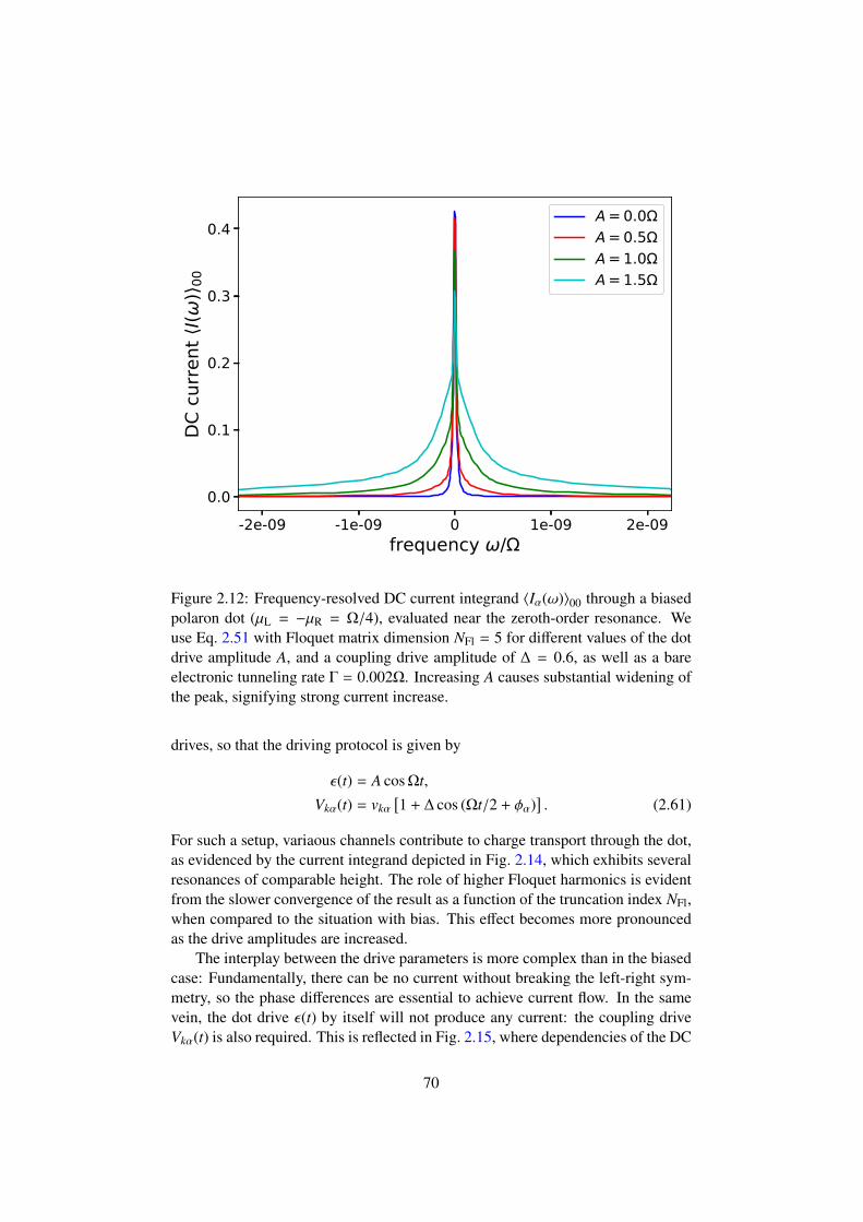
-2e-09 -1e-09 0 1e-09 2e-09frequency /
0.0
0.1
0.2
0.3
0.4
DC c
urre
nt I
() 0
0A = 0.0A = 0.5A = 1.0A = 1.5
Figure 2.12: Frequency-resolved DC current integrand 〈Iα(ω)〉00 through a biasedpolaron dot (µL = −µR = Ω/4), evaluated near the zeroth-order resonance. Weuse Eq. 2.51 with Floquet matrix dimension NFl = 5 for different values of the dotdrive amplitude A, and a coupling drive amplitude of ∆ = 0.6, as well as a bareelectronic tunneling rate Γ = 0.002Ω. Increasing A causes substantial widening ofthe peak, signifying strong current increase.
drives, so that the driving protocol is given by
ε(t) = A cos Ωt,
Vkα(t) = vkα[1 + ∆ cos (Ωt/2 + φα)
]. (2.61)
For such a setup, variaous channels contribute to charge transport through the dot,as evidenced by the current integrand depicted in Fig. 2.14, which exhibits severalresonances of comparable height. The role of higher Floquet harmonics is evidentfrom the slower convergence of the result as a function of the truncation index NFl,when compared to the situation with bias. This effect becomes more pronouncedas the drive amplitudes are increased.
The interplay between the drive parameters is more complex than in the biasedcase: Fundamentally, there can be no current without breaking the left-right sym-metry, so the phase differences are essential to achieve current flow. In the samevein, the dot drive ε(t) by itself will not produce any current: the coupling driveVkα(t) is also required. This is reflected in Fig. 2.15, where dependencies of the DC
70
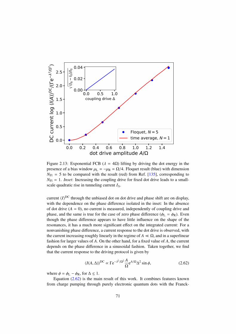
0.0 0.2 0.4 0.6 0.8 1.0 1.2 1.4dot drive amplitude A/
0.0
0.5
1.0
1.5
2.0
2.5
DC c
urre
nt lo
g I(A
)DC/(
e2 /
2 )
Floquet, N = 5time average, N = 1
0.0 0.5 1.0coupling drive
0.00
0.02
0.04(I
I 0)/I
0
Figure 2.13: Exponential FCB (λ = 4Ω) lifting by driving the dot energy in thepresence of a bias window µL = −µR = Ω/4. Floquet result (blue) with dimensionNFl = 5 to be compared with the result (red) from Ref. [135], corresponding toNFl = 1. Inset: Increasing the coupling drive for fixed dot drive leads to a small-scale quadratic rise in tunneling current I∆.
current 〈I〉DC through the unbiased dot on dot drive and phase shift are on display,with the dependence on the phase difference isolated in the inset: In the absenceof dot drive (A = 0), no current is measured, independently of coupling drive andphase, and the same is true for the case of zero phase difference (φL = φR). Eventhough the phase difference appears to have little influence on the shape of theresonances, it has a much more significant effect on the integrated current: For anonvanishing phase difference, a current response to the dot drive is observed, withthe current increasing roughly linearly in the regime of A Ω, and in a superlinearfashion for larger values of A. On the other hand, for a fixed value of A, the currentdepends on the phase difference in a sinusoidal fashion. Taken together, we findthat the current response to the driving protocol is given by
〈I(A,∆)〉DC ∝ Γe−λ2/Ω2 A
ΩeA/Ω∆2 sin φ, (2.62)
where φ = φL − φR, for ∆ . 1.Equation (2.62) is the main result of this work. It combines features known
from charge pumping through purely electronic quantum dots with the Franck-
71
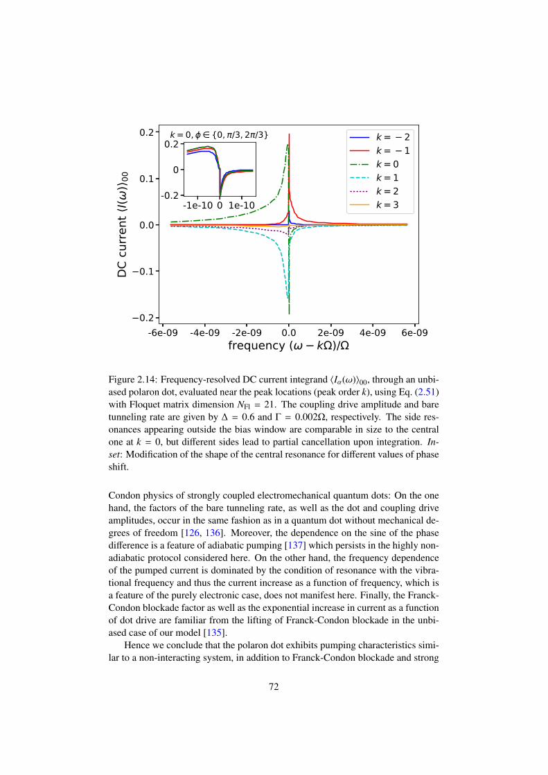
-6e-09 -4e-09 -2e-09 0.0 2e-09 4e-09 6e-09frequency ( k )/
0.2
0.1
0.0
0.1
0.2DC
cur
rent
I(
) 00
k = 2k = 1k = 0k = 1k = 2k = 3-1e-10 0 1e-10
-0.2
0
0.2k = 0, 0, /3, 2 /3
Figure 2.14: Frequency-resolved DC current integrand 〈Iα(ω)〉00, through an unbi-ased polaron dot, evaluated near the peak locations (peak order k), using Eq. (2.51)with Floquet matrix dimension NFl = 21. The coupling drive amplitude and baretunneling rate are given by ∆ = 0.6 and Γ = 0.002Ω, respectively. The side res-onances appearing outside the bias window are comparable in size to the centralone at k = 0, but different sides lead to partial cancellation upon integration. In-set: Modification of the shape of the central resonance for different values of phaseshift.
Condon physics of strongly coupled electromechanical quantum dots: On the onehand, the factors of the bare tunneling rate, as well as the dot and coupling driveamplitudes, occur in the same fashion as in a quantum dot without mechanical de-grees of freedom [126, 136]. Moreover, the dependence on the sine of the phasedifference is a feature of adiabatic pumping [137] which persists in the highly non-adiabatic protocol considered here. On the other hand, the frequency dependenceof the pumped current is dominated by the condition of resonance with the vibra-tional frequency and thus the current increase as a function of frequency, which isa feature of the purely electronic case, does not manifest here. Finally, the Franck-Condon blockade factor as well as the exponential increase in current as a functionof dot drive are familiar from the lifting of Franck-Condon blockade in the unbi-ased case of our model [135].
Hence we conclude that the polaron dot exhibits pumping characteristics simi-lar to a non-interacting system, in addition to Franck-Condon blockade and strong
72
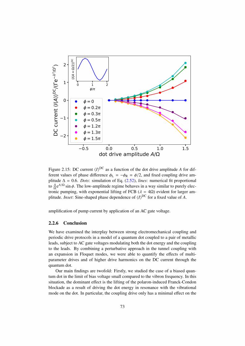
0.5 0.0 0.5 1.0 1.5dot drive amplitude A/
2
1
0
1
2
DC c
urre
nt I
(A)DC
/(e
2 /2 )
= 0= 0.2= 0.3= 0.5= 1.2= 1.3= 1.5
0 1 2/
I(A=
/2)DC
Figure 2.15: DC current 〈I〉DC as a function of the dot drive amplitude A for dif-ferent values of phase difference φL = −φR = φ/2, and fixed coupling drive am-plitude ∆ = 0.6. Dots: simulation of Eq. (2.52), lines: numerical fit proportionalto A
ΩeA/Ω sin φ. The low-amplitude regime behaves in a way similar to purely elec-
tronic pumping, with exponential lifting of FCB (λ = 4Ω) evident for larger am-plitude. Inset: Sine-shaped phase dependence of 〈I〉DC for a fixed value of A.
amplification of pump current by application of an AC gate voltage.
2.2.6 Conclusion
We have examined the interplay between strong electromechanical coupling andperiodic drive protocols in a model of a quantum dot coupled to a pair of metallicleads, subject to AC gate voltages modulating both the dot energy and the couplingto the leads. By combining a perturbative approach in the tunnel coupling withan expansion in Floquet modes, we were able to quantify the effects of multi-parameter drives and of higher drive harmonics on the DC current through thequantum dot.
Our main findings are twofold: Firstly, we studied the case of a biased quan-tum dot in the limit of bias voltage small compared to the vibron frequency. In thissituation, the dominant effect is the lifting of the polaron-induced Franck-Condonblockade as a result of driving the dot energy in resonance with the vibrationalmode on the dot. In particular, the coupling drive only has a minimal effect on the
73
current in this regime, and the current response to the drive is well approximatedby the Floquet component which encodes time-averaged contributions. This re-sult also serves to confirm earlier work on drive-induced lifting of Franck-Condonblockade, where only time-averaged correlation functions were considered in theperturbative expansion [135].
Secondly, we applied the same formalism to the unbiased quantum dot. There,the interplay between both dot and coupling drives makes it possible to pump aDC current through the system: Similar to the case of charge pumping in purelyelectronic systems, we find that in the regime of weak dot drive the DC currentflow is approximately proportional to the drive amplitude, as long as a phase dif-ference between the left and right coupling drives is employed to break left-rightsymmetry. The dependence of the current on this phase is found to always be si-nusoidal, irrespective of the dot drive amplitude. In the regime of strong dot drive,in contrast, the current response becomes superlinear and approximates the expo-nential characteristic found in the biased quantum dot. Thus, the driven unbiasedpolaron quantum dot combines the exponential lifting of Franck-Condon blockadewith features of adiabatic charge pumping through purely electronic systems, evenfar away from the adiabatic limit.
As recent experiments have used electronic gates to localize quantum dots oncarbon nanotubes, we anticipate that these could also be employed to supply the ACvoltages we use to predict charge pumping, thus providing an implementation ofour model and adding to the versatility of carbon nanotubes as elements of circuitry.Moreover, the Anderson-Holstein Hamiltonian used in this work is a fairly generalmodel and could be realized in multiple ways, as long as there is a way to engineerstrong coupling between a fermion and a bosonic mode and subject this system toseveral resonant drives. In particular, an optomechanical implementation could beenvisioned, with cavity modes taking the role of the drive.
The model itself can be extended to include multiple electron levels and os-cillator modes by replacing the expression for the dot Green’s function by a morecomplex one; this appears as a promising way to better capture the possible com-plexities of experiments. Furthermore, the generality of the Floquet formalismalso permits the consideration of more complex driving schemes as well as thetime-dependent current response. Finally, while the polaron tunneling approxima-tion allows to simplify the diagrammatic expansion substantially and yet capturethe effect of electron-phonon interaction in the parameter ranges considered in thiswork, it would be interesting to explore alternatives such as the Floquet DMFT[55], which would allow to move beyond this approximation, as well as to con-sider more complex system Hamiltonians.
2.2.7 Appendix: Bare Green’s functions
Here, we derive the expressions Eq. (2.56) and Eq. (2.57) for the bare and free dotGreen’s functions. The free dot Green’s function is calculated by evolution withthe time independent Hamiltonian Hfree
0 = εd†d + Ωa†a and factors into electronic
74
and vibrational parts,
Dfree0 (τ, τ′) = −i
⟨TCd(τ)d†(τ′)
⟩free
0
⟨TCX(τ)X†(τ′)
⟩free
0, (2.63)
where X(τ) = e−λ2
Ω2 (a†eiΩτ−ae−iΩτ). Using Keldysh matrix notation, the electronicGreen’s function takes shape as
⟨TCd(τ)d†(τ′)
⟩free
0= e−iε(t−t′)
(−N0 + θ(t − t′) −N0
1 − N0 −N0 + θ(t′ − t)
). (2.64)
Throughout this work, we focus on times beyond the transient regime, meaning theeffect of the initial dot occupation N0 is negligible and can hence be set to N0 = 0.On the other hand, the vibrational part reads
⟨TCX(τ)X†(τ′)
⟩free
0= e−λ
2/Ω2
eλ2
Ω2 e−iΩ|t|eλ2
Ω2 eiΩt
eλ2
Ω2 e−iΩteλ2
Ω2 eiΩ|t|
. (2.65)
The retarded component in Eq. (2.57) is obtained by Fourier transform of Eq. (2.63)and using the definition
(Dfree
0
)R
0=
(Dfree
0
)−−−
(Dfree
0
)−+.
The bare dot Green’s function differs from the free one by the additional evo-lution with the drive Hamiltonian Hdr(t) = A cos Ωε t, which implies
D0(τ, τ′) = Dfree0 (τ, τ′)e−i A
Ωε(sin Ωετ−sin Ωετ
′)
=∑n∈Z
einΩετav Dfree0 (τrel)inJn
(−
2AΩε
sinΩετrel
2
), (2.66)
where Jn denotes the n-th Bessel function of the first kind. By Fourier transformingin the relative time coordinate, we obtain the Wigner expansion,∫ ∞
−∞
dτreleiωτrel inJn
(−
2AΩε
sinΩετrel
2
)=
∫ ∞
−∞
dτreleiωτrel in∑m≥0
(−1)m
m!(m + n)!
(−
AΩε
sinΩετrel
2
)2m+n
=
∫ ∞
−∞
dτreleiωτrel in∑m≥0
(−1)m
m!(m + n)!
(−
Ai2Ωε
)2m+n (ei Ωε τrel
2 − e−i Ωε τrel2
)2m+n
=
∫ ∞
−∞
dτrel
∑m≥0
2m+n∑k=0
ei(ω+kΩε−mΩε−n2 Ωε)τrel
(−1)k
m!(m + n)!
(A
2Ωε
)2m+n (2m + n
k
)
= 2π∑m≥0
2m+n∑k=0
δ(ω −
(m +
n2− k
)Ωε
) (−1)k
m!(m + n)!
(A
2Ωε
)2m+n (2m + n
k
). (2.67)
75
This expression is then convolved with Dfree0 (ω):
D0(tav, trel) =∑n∈Z
einΩε tav
∫ ∞
−∞
dω2π
e−iωtrel
∑m≥0
2m+n∑k=0
Dfree0
(ω −
(m +
n2− k
)Ωε
)λmk
n , (2.68)
with
λmkn =
(−1)k
m!(m + n)!
(A
2Ωε
)2m+n (2m + n
k
). (2.69)
2.2.8 Appendix: Self-energy
In the following, we give the derivations of the mode expansions Eq. (2.58) andEq. (2.59) for the retarded and lesser component of the lead self-energy, respec-tively. Resummation of the perturbation series for D(τ, τ′) produces the Dysonequation (2.45), with a self-energy Σ which contains the time dependence of thecoupling Vkα(t) = vkα
[1 + ∆ cos (ΩV t + φα)
],
Σ(τ1, τ2) =∑kα
Vkα(τ1)V∗kα(τ2)Gkα(τ1, τ2). (2.70)
Introducing Wigner coordinates and Fourier transforming, we obtain
Σ(tav, ω)α =∑
k
|vkα|2∫ ∞
−∞
dtreleiωtrelVkα(tav + trel/2)V∗kα(tav − trel/2)Gkα(trel)
=∑
k
|vkα|2∫ ∞
−∞
dtreleiωtrel
[|∆|2
4e−i2φαGkα(trel)e−i2ΩV tav +
|∆|2
4ei2φαGkα(trel)ei2ΩV tav
+
(1 +|∆|2
4eiΩV trel +
|∆|2
4e−iΩV trel
)Gkα(trel)
+
(∆
2ei(ΩV trel/2+φα) +
∆∗
2ei(−ΩV trel/2+φα)
)Gkα(trel)eiΩV tav
+
(∆
2e−i(ΩV trel/2+φα) +
∆∗
2e−i(−ΩV trel/2+φα)
)Gkα(trel)e−iΩV tav
]. (2.71)
In order to obtain the retarded and lesser components of the self energy, we substi-tute the free lead Green’s functions
GRkα(trel) = −iθ(trel)e−iεkαtrel ,
G−+kα (trel) = inF(εkα)e−iεkαtrel , (2.72)
respectively. Using the identity limη→0+(ω−εkα+iη)−1 = P(ω−εkα)−1−iπδ(ω−εkα),with the notation P for the principal value, the integral is readily performed. In thewide-band limit, the bare electronic tunneling rate Γ = 2π
∑k |vkα|
2δ(ω− εkα) is setto be independent of frequency, which yields Eqs. (2.58) and (2.59).
76
2.3 Quantum thermodynamics of the resonant-level modelwith driven system-bath coupling
We study nonequilibrium thermodynamics in a fermionic resonant-level model witharbitrary coupling strength to a fermionic bath, taking the wide-band limit. In con-trast to previous theories, we consider a system where both the level energy and thecoupling strength depend explicitly on time. We find that, even in this generalizedmodel, consistent thermodynamic laws can be obtained, up to the second orderin the drive speed, by splitting the coupling energy symmetrically between systemand bath. We define observables for the system energy, work, heat, and entropy,and calculate them using nonequilibrium Green’s functions. We find that the ob-servables fulfill the laws of thermodynamics, and connect smoothly to the knownequilibrium results. This section is based on the article Quantum thermodynamicsof the resonant-level model with driven system-bath coupling, written in collab-oration with Massimiliano Esposito and Thomas L. Schmidt, published in Phys.Rev. B 97, 085435 (2018).
2.3.1 Introduction
Thermodynamics has long been central to the understanding and optimization ofthe performance of work cycles and machines. As a result of recent advances infabrication technology and measurement techniques, the range of realizable ma-chines now extends down to the size of a single molecule [97, 138, 139, 140]. Atthis length scale, many of the assumptions underlying the edifice of thermodynam-ics are no longer valid. Specifically, the paradigm of a nanoscale system coupledto a bath features a variety of subtleties that are not present in macroscopic setups.First, the extent of the contact area between system and bath may be similar to thatof the system itself, meaning the details of the coupling become relevant and canno longer be treated in the same general fashion as in the macroscopic case. Sec-ond, if the coupling is of sufficient strength, even the distinction between systemand bath may itself become blurred [141]. Finally, the task of taking into accountnonequilibrium effects is much more intricate at the nanoscale and has received agreat deal of recent attention. These difficulties are compounded by quantum ef-fects that play no role macroscopically but rise to prominence in small systems.However, even the problem of formulating a microscopic theory of nonequilibriumthermodynamics for a classical system is daunting in itself [90, 142, 86, 143].
The key to establishing a framework of nonequilibrium quantum thermody-namics is to define quantities that transfer the concepts of system energy, entropy,heat, and work to the nanoscale regime in the context of a given system, while pre-serving as much generality as possible. To this end, a wide variety of approacheshas been pursued, studying setups which roughly fall into the two categories ofweak [67, 57, 73, 69, 144] and general couplings [70, 85, 80, 73, 145, 146, 74,147, 148, 149, 150] between system and bath, respectively. For the case of weakcoupling, consistent thermodynamics has been established [57, 73, 69, 151], as
77
outlined in Sec. 1.5.1, but beyond weak coupling, the situation is much less clear:There, the meaning of work and work fluctuations has been understood, but thequest for definitions of system energy and heat remains open [70, 80, 74].
Recently, the formalism of nonequilibrium Green’s functions has been appliedto the question of statistical physics and thermodynamics in paradigmatic quan-tum systems [152]. The advantage of this approach lies in its inherent ability totreat both nonequilibrium and strong-coupling situations, meaning that Green’sfunctions can readily provide a wide range of candidates for thermodynamic def-initions. The subjects of these studies are variants of the resonant-level model,consisting of an electronic level coupled to metallic leads, under the influence ofa drive protocol. This constitutes a minimal description of a quantum dot coupledto source and drain electrodes and driven by means of AC gate voltages. Elec-tronic transport in the time-dependent resonant-level model and its extensions hasbeen studied for several years [153, 154, 34, 135, 155], but more recently its ther-modynamic properties have come into the spotlight. Several sets of thermody-namic definitions have been proposed in this way, with varying ranges of validity[156, 157, 158, 159, 160, 161, 162, 163, 164]. In particular, it has proved chal-lenging to find appropriate generalizations of corresponding equilibrium quantities[158], and to incorporate drive protocols and coupling structures of general form[160, 161].
Our work considers a resonant-level model in the spirit of Ref. [160], wherethe electron level is subjected to a time-dependent drive and coupled to a singlelead, which we consider in the wide-band limit. To arrive at a more realistic modelfor experiments [165], we extend the existing models by in addition allowing fora time-dependent coupling between system and bath, and show that it admits ananalytical solution in terms of Green’s functions. These solutions give rise tononequilibrium thermodynamic quantities, which connect smoothly to their equi-librium counterparts, and obey the laws of thermodynamics in the quasi-adiabaticlimit. In doing so, we give a definition of the heat current which differs from thoseconsidered in Ref. [157] and thus resolve the apparent inconsistency caused bytime-dependent coupling.
The paper is structured as follows: In Sec. 2.3.2, we introduce the resonant-level model and its solution in the presence of time-dependent parameters. Next,we use this solution to define thermodynamic quantities in Sec. 2.3.3, and demon-strate the first law of thermodynamics in our model. We proceed in Sec. 2.3.4 byconfirming that the adiabatic limit of our definitions matches established equilib-rium results. In Sec. 2.3.5 we perform an expansion in derivatives of the driveprotocol, from which we conclude that our definitions are compatible with the sec-ond law of thermodynamics up to second order in drive velocities. We comparethis expansion with exact numerical results in Sec. 2.3.6. Finally, we summarizeour findings and compare to related results in the literature, in Sec. 2.3.7.
78
2.3.2 Resonant-level model
We study a model Hamiltonian for a single electronic level coupled to a fermioniclead of length L,
H(t) = HD(t) + HB + HT(t), (2.73)
HD(t) = ε(t)d†d,
HB =∑
k
εkc†kck,
HT(t) =∑
k
γ(t)√
Ld†ck + h. c.,
where HD(t), HB, and HT(t) are the dot, lead, and tunneling Hamiltonians, re-spectively. Here, d† and d denote the creation and annihilation operators for thedot electron and fulfill the fermionic commutation relation d, d† = 1. Analo-gously, the operators c†k and ck are associated with the lead electrons, with theindex k enumerating the lead modes. In the absence of the tunneling term, weassume thermal equilibrium in the lead, thus imposing 〈c†kcq〉0 = δkqnF(εk), wherenF(εk) = [1+eβ(εk−µ)]−1 denotes the Fermi-Dirac distribution at inverse temperatureβ with chemical potential µ, and the subscript 0 denotes expectation values takenwith respect to the quadratic Hamiltonian HD(t) + HB. Both the dot energy ε(t)and the dot-lead coupling strength γ(t) are subject to time-dependent drive, and noassumption is made regarding the magnitude of γ(t). In this way, the Hamiltonianin Eq. (2.73) combines nonequilibrium physics and potentially strong coupling be-tween system and bath, and hence features several of the challenges inherent in theattempt to formulate quantum thermodynamics. The schematics of the model arevisualized in Fig. 2.16.
In the following, we describe the dynamics of the resonant-level model ofEq. (2.73) in terms of nonequilibrium Green’s functions [47], which can be cal-culated analytically, as laid out in Sec. 1.2. Specifically, we consider the tunnelingHamiltonian HT in the role of the interaction, and use a perturbation series to cap-ture the renormalization of dot properties as a consequence of this interaction.
Resumming the perturbation series leads to a Dyson equation for the full dotGreen’s function as in Eq. (1.34),
D(τ, τ′) = D0(τ, τ′) +
∫C
dσdσ′D0(τ, σ)Σ(σ,σ′)D(σ′, τ′), (2.74)
as a function of the bare dot Green’s function D0(τ, τ′) = −i〈d(τ)d†(τ′)〉0. Thus,the consequences of coupling to the leads are fully quantified by the self-energy,which is given by
Σ(σ,σ′) =γ(σ)γ∗(σ′)
L
∑k
G0,k(σ,σ′), (2.75)
79
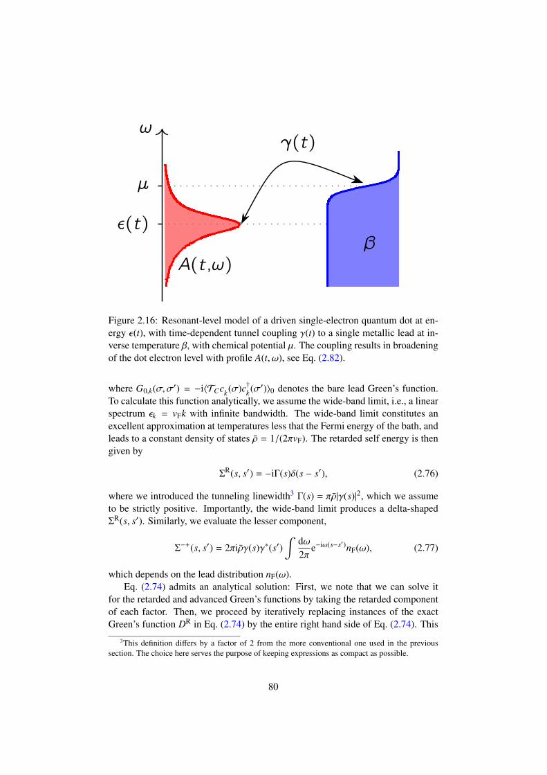
ω
µ
ε(t)
γ(t)
A(t,ω)β
Figure 2.16: Resonant-level model of a driven single-electron quantum dot at en-ergy ε(t), with time-dependent tunnel coupling γ(t) to a single metallic lead at in-verse temperature β, with chemical potential µ. The coupling results in broadeningof the dot electron level with profile A(t, ω), see Eq. (2.82).
where G0,k(σ,σ′) = −i〈TCck(σ)c†k(σ′)〉0 denotes the bare lead Green’s function.To calculate this function analytically, we assume the wide-band limit, i.e., a linearspectrum εk = vFk with infinite bandwidth. The wide-band limit constitutes anexcellent approximation at temperatures less that the Fermi energy of the bath, andleads to a constant density of states ρ = 1/(2πvF). The retarded self energy is thengiven by
ΣR(s, s′) = −iΓ(s)δ(s − s′), (2.76)
where we introduced the tunneling linewidth3 Γ(s) = πρ|γ(s)|2, which we assumeto be strictly positive. Importantly, the wide-band limit produces a delta-shapedΣR(s, s′). Similarly, we evaluate the lesser component,
Σ−+(s, s′) = 2πiργ(s)γ∗(s′)∫
dω2π
e−iω(s−s′)nF(ω), (2.77)
which depends on the lead distribution nF(ω).Eq. (2.74) admits an analytical solution: First, we note that we can solve it
for the retarded and advanced Green’s functions by taking the retarded componentof each factor. Then, we proceed by iteratively replacing instances of the exactGreen’s function DR in Eq. (2.74) by the entire right hand side of Eq. (2.74). This
3This definition differs by a factor of 2 from the more conventional one used in the previoussection. The choice here serves the purpose of keeping expressions as compact as possible.
80
leads to an expansion in powers of the self-energy, which sums to
DR(t, t′) = −iθ(t − t′)e−i∫ t
t′ dsε(s)e−∫ t
t′ dsΓ(s). (2.78)
The advanced component is then given by DA(t, t′) = DR(t′, t)∗. Together with thelesser self-energy, they give rise to the D−+ via the Langreth rule, Eq. (1.51),
D−+(t, t′) =
∫ ∞
−∞
ds ds′DR(t, s)Σ−+(s, s′)DA(s′, t′), (2.79)
which we simplified by noting that an additional term [47], which is proportional tothe dot occupation at the initial time t0, drops out since t0 → −∞. Using Eqs. (2.77)and (2.78), we thus evaluate the lesser dot Green’s function as
D−+(t, t′) = 2i∫
dω2π
nF(ω)e−iω(t−t′)V(t, ω)V∗(t′, ω), (2.80)
where we defined the function
V(t, ω) =
∫ t
−∞
ds√
Γ(s) exp∫ t
sdy
[iω − iε(y) − Γ(y)
](2.81)
which encodes the history of the driving protocol [ε(t),Γ(t)]. This result is in agree-ment with the findings of an equation-of-motion approach [153]. By choosingt = t′, this Green’s function provides us with the expectation value of the dot par-ticle number, N(t) = −iD−+(t, t),
N(t) =
∫dω2π
nF(ω)A(t, ω), (2.82)
where we wrote
A(t, ω) = 2|V(t, ω)|2. (2.83)
Note that Eq. (2.82) appears as a straightforward generalization of the dot particlenumber in a stationary system, where A(t, ω) would be replaced by the Lorentzianspectral function
A0(ω) =2Γ
(ω − ε)2 + Γ2 . (2.84)
Since it can be shown that in the stationary case A and A0 coincide (see App. 2.3.8),the expression A(t, ω) can be viewed as a drive-induced modification of the dotspectral function. However, it bears pointing out that in general A does not matchthe definition of the non-stationary spectral function: A(t, ω) , −2 Im DR(t, ω),where DR(t, ω) stands for the Wigner transform of the retarded dot Green’s func-tion.
We have thus arrived at a fully analytical solution of the resonant-level modelin the presence of two drives, after taking the wide-band limit. In a way similar tothe particle number, expectation values of any other operator on the dot and leadHilbert spaces can be calculated from the Green’s function matrix D(t, t′).
81
2.3.3 Thermodynamic definitions and first law
In the following, we define thermodynamic quantities for our system in terms ofquantum mechanical expectation values and use the Green’s functions obtained inthe previous section to calculate them. Herein, we require these definitions to becompatible with the laws of thermodynamics, in the presence of dot and couplingdrives as well as arbitrary dot-lead coupling strength.
It has been shown previously [156, 160] that for the case of time-independentcoupling, such a set of definitions may be obtained by defining a system energythat consists of the expectation value of the dot Hamiltonian with half the couplingHamiltonian added,
ES(t) =
⟨HD(t) +
12
HT(t)⟩. (2.85)
This kind of splitting is indicative of the fact that in the presence of strong coupling,one cannot simply identify the dot with the “system”, and the lead with the “bath”,in the thermodynamic sense of these terms. Moreover, energy added to the totalensemble by the coupling drive must be partitioned between system and bath. Thechoice of a partition factor of 1/2 has the added feature that the system energy canthen be written as an expectation value of dot operators only, ES = −i〈∂td†d −d†∂td〉/2. In the following, we show that, even in the case of driven coupling, thischoice of system energy conforms to the first and second laws of thermodynamics.
The expectation values in Eq. (2.85) are readily expressed in terms of Green’sfunctions, leading to the exact result
ES(t) =
∫dω2πωnF(ω)A(t, ω)
− 2∫
dω2π
nF(ω) Im[∂tV(t, ω)V∗(t, ω)
], (2.86)
with V(t, ω) and A(t, ω) as in Eqs. (2.81) and (2.83). We define the rate of changein work performed on the system as split into three parts,
W(t) ≡ WSB(t) + WC(t) + WB(t), (2.87)
where WSB(t) = 〈∂tH(t)〉 and WC(t) = µ∂tN(t) denote the power supplied by thedrive to system and bath, and the chemical work rate associated with particle flowinto the dot, respectively. Below, we will always use the dot symbol to denote arate, as opposed to ∂t which stands for a time derivative. WSB(t) is found to be
WSB(t) = ∂tε(t)N(t) + 〈∂tHT(t)〉
= ∂tε(t)∫
dω2π
nF(ω)A(t, ω) +2∂tΓ(t)√
Γ(t)
∫dω2π
nF(ω) Im V(t, ω), (2.88)
whereas the chemical chemical work rate equals
WC(t) = 4µ√
Γ(t)∫
dω2π
nF(ω) Re V(t, ω) − 2µΓ(t)∫
dω2π
nF(ω)A(t, ω). (2.89)
82
The third term in Eq. (2.87) is a work done by the system-bath coupling to changethe particle numbers in the bath. It is reminiscent of the work that the couplingneeds to do to create a volume in the bath recently identified in Ref. [86], but inthe grand canonical ensemble. In order to obtain the rate of work performed on thesystem only, this contribution therefore needs to be subtracted. It is given by
WB(t) ≡1π∂tΓ(t) = 2∂tΓ(t)∂µNeq
B /ρ, (2.90)
where ρ is the lead density of states as in Sec. 2.3.2 and NeqB = ρ
∫dω2π nF(ω) denotes
the (infinite) equilibrium particle number in the lead. Its change with respect tothe chemical potential, ∂µNeq
B , is finite and can be seen as the grand canonicalanalogue of a compressibility. One sees therefore that WB arises from changes inthe tunneling linewidth Γ(t) which modify the level repulsion among the levels inthe lead, in turn causing a change in the lead particle number.
Among the results of Sec. 2.3.5, we will find that this definition of WB is com-patible with the second law of thermodynamics. Lastly, we define the heat currentflowing into the system as
Q(t) = −∂t
⟨HB +
12
HT(t)⟩− WC(t) − WB(t). (2.91)
Mirroring Eq. (2.85), this definition associates half of the coupling energy with thebath, and explicitly features the reversed work flows due to particle transfer andwork performed on the bath. Our notion of heat flow presents a generalization ofthe one used in Ref. [156] for time-dependent coupling, which differs from the oneconsidered in Ref. [157].
If we sum up the definitions from Eqs. (2.85), (2.87), and (2.91), we obtain theenergy balance
∂tES = Q + W, (2.92)
which makes manifest the first law of thermodynamics in our system, with E takingon the role of the internal energy.
2.3.4 Link to equilibrium
In this section, we show that the definitions made in Sec. 2.3.3 are compatible withthe concept of the Hamiltonian of mean force as discussed in Sec. 1.5.3. We startby defining a potential of mean force for the adiabatic limit of our model. Thenwe take the limit of infinitely slow drive, ∂tε → 0 and ∂tΓ → 0 of the definitionsmade in Sec. 2.3.3 and find that the two approaches coincide, thus ensuring thatour quantities reduce to the correct adiabatic limit.
We can view Eq. (1.125) as the starting point for the mean-force approach:There, a thermodynamic potential for the system (dot) is defined by as the differ-ence of the corresponding potential for the “super-system” comprising both dot and
83
lead, and that of the lead itself. Here, we choose to work in the grand canonical en-semble that is characterized by a fixed inverse temperature β and chemical potentialµ, in analogy to our Green’s function approach. The grand canonical ensemble ofthe super-system is realized by weak coupling to a “super-bath”, thus fixing β andµ for the ensemble. This setup has been employed for a classical model [142], aswell as for the resonant-level model with a single drive parameter [160].
In the absence of drive, and assuming that the super-system is coupled to thesuper-bath in a fashion permitting energy and particle exchange, we can obtain theweak coupling thermodynamics of the super-system from the equilibrium grandcanonical potential
Ωeq ≡ −1β
log tr e−β(H−µN)
= −1β
∫dω2πρ(ω) log
(1 + e−β(ω−µ)
)(2.93)
where N is the particle number operator of the super-system. Here, ρ(ω) denotesthe stationary density of states of the super-system. It is defined as the sum of dotand lead contributions, which in terms of Green’s functions is given by
ρ(ω) = −2 Im DR(ω) − 2∑
k
Im GRk (ω). (2.94)
Following Ref. [160], we note that the sum over the exact lead Green’s functionsobeys the Dyson equation∑
k
GRk (ω) =
∑k
GR0,k(ω) + |γ|2DR(ω)
∑k
[GR
0,k(ω)]2. (2.95)
Writing the unperturbed lead Green’s function in the frequency domain, GR0,k(ω) =
(ω − εk + i0+)−1, we see that the correction becomes
|γ|2DR(ω)∑
k
[GR
0,k(ω)]2
= −DR(ω)∂ω
|γ|2 ∑k
GR0,k(ω)
= −DR(ω)∂ωΣR(ω) (2.96)
According to Eq. (2.76), this correction vanishes in the wide-band limit. Thereforethe lead component of ρ(ω) is not renormalized by the coupling, facilitating itsinterpretation as a “pure bath” term which does not contribute to the system ther-modynamics and is subtracted from Eq. (2.93) in the sense of Eq. (1.125). We thusdefine the (system) grand canonical potential of mean force,
ΩeqS ≡ −
1β
∫dω2π
A0(ω) log(1 + e−β(ω−µ)
), (2.97)
84
where A0(ω) is the stationary spectral function defined in Eq. (2.84). Changes inΩ
eqS resulting from modification of the system parameters are equal to the corre-
sponding changes in Ωeq. With this choice of ΩeqS , we can use equilibrium ther-
modynamics to obtain expressions for the equilibrium values of particle number,system entropy and energy,
Neq = −∂µΩeqS =
∫dω2π
A0(ω)nF(ω) (2.98)
S eq = −∂T ΩeqS =
∫dω2π
A0(ω)σF(ω) (2.99)
EeqS = Ω
eqS + µNeq +
1β
S eq =
∫dω2π
A0(ω)ωnF(ω). (2.100)
where in Eq. (2.99) we defined the frequency-resolved entropy factor
σF(ω) = −nF(ω) log nF(ω) − [1 − nF(ω)] log [1 − nF(ω)]. (2.101)
These quantities can be related to the adiabatic limit of the definitions in Sec. 2.3.3by introducing a parametric time dependence in A0 via ε(t) and Γ(t). The ex-pressions obtained by substituting this time-dependent Lorentzian A0(t, ω) intoEqs. (2.98), (2.99), and (2.100) can then be used to calculate the adiabatic particleand energy currents,
∂tNeq(t) =
∫dω2π
nF (∂ΓA0∂tΓ + ∂εA0∂tε) = [∂tN](1)
∂tEeqS (t) =
∫dω2πω f (∂ΓA0∂tΓ + ∂εA0∂tε) = [∂tE](1), (2.102)
where the right hand sides refer to the adiabatic expansions of the time derivativesof Eqs. (2.82) and (2.86), respectively, which are detailed in App. 2.3.9. Similarly,we can interpret the time derivative of the grand canonical potential as the rate ofmechanical work performed on the system,
∂tΩeqS (t) = −
1β
∫dω2π
(∂ΓA0∂tΓ + ∂εA0∂tε)[σF(ω) − β(ω − µ)nF(ω)
]= W (1)
SB + WB, (2.103)
as can be gleaned from Eq. (2.127). Hence we conclude that the adiabatic limitof the system quantities defined in Sec. 2.3.3 matches the result of adiabatic weakcoupling thermodynamics as encoded in the grand canonical potential of meanforce from Eq. (2.97).
2.3.5 Second law
Having obtained a definition for the heat flowing into the system, we now addressthe question of how to define the system entropy. To this end, we generalize the
85
adiabatic expression given in Eq. (2.99) and show the compatibility of this choicewith the previous definitions by exhibiting the second law.
In analogy to the non-adiabatic result for the particle number on the dot, Eq. (2.82),we define the system entropy beyond the adiabatic limit by replacing the Lorentzianspectral function A0 in Eq. (2.99) with the function A as in Sec. 2.3.2,
S (t) ≡∫
dω2π
A(t, ω)σF(ω). (2.104)
Next, we show the second law in the sense that the entropy production rate is non-negative up to second order in the quasi-adiabatic expansion:
∂tS − βQ ≥ 0, (2.105)
with equality up to first order. Details of the expansion can be found in App. 2.3.9.Starting with the first order, we note that on the one hand, the derivative of
Eq. (2.104) is approximated by
[∂tS ](1) =
∫dω2πσF(ω) (∂ΓA0∂tΓ + ∂εA0∂tε) , (2.106)
whereas on the other hand, we obtain the corresponding terms for the heat flowfrom Eq. (2.127),
Q(1) =1β
∫dω2πσF (∂ΓA0∂tΓ + ∂εA0∂tε)
−1β
∫dω2π
log(1 + e−βω
)∂ω
(−ω − ε
ΓA0∂tΓ − A0∂tε
)−
∫dω2π
nFA0
(ω − ε
Γ∂tΓ + ∂tε
)− WB. (2.107)
An integration by parts in the second integral yields a term that cancels the third in-tegral, as well as a boundary contribution equal to ∂tΓ/π, thus canceling −WB. Thefirst integral coincides with [∂tS ](1), which implies that to first order in adiabaticexpansion, the change in system entropy is entirely due to heat flow,
[∂tS ](1) = βQ(1). (2.108)
Moreover, the quasi-adiabatic expansion shows that our definitions give rise toexact differentials for the system energy as well as reversible work and heat flowsto first order in time derivatives,
∂Γ∂ε Q(1) = ∂ε∂ΓQ(1),
∂Γ∂εW(1) = ∂ε∂ΓW (1). (2.109)
In particular, the reversible heat therefore fulfills the requirement of being a statefunction. This should be contrasted with the observation made in Ref. [157], that a
86
certain class of heat definitions, arising from a splitting of the coupling energy as inEq. (2.85), fails to exhibit this property as soon as driven coupling is introduced. Asour choice of Q from Eq. (2.91) differs from the class of heat definitions consideredin Ref. [157], this problem does not arise here.
Moving to the second order in time derivatives, we note that the relevant partof Q(2) are given by the last two integrals in Eq. (2.126),
δQ(2) ≡ Q(2) − Q(1)
=Γ2
2
∫dω2π∂ωnFA2
0
(∂tω − ε
Γ
)2
+
∫dω2π
(ω − µ)∂ωnF∂t
A20Γ
2∂tω − ε
Γ
. (2.110)
On the other hand, the expansion of ∂tS is immediate from Eq. (2.121),
δS (2) ≡ [∂tS ](2) − [∂tS ](1)
=
∫dω2π∂ωσF∂t
A20Γ
2∂tω − ε
Γ
. (2.111)
Using ∂ωσF(ω) = β(ω − µ)∂ω f , we see that this matches the second term inEq. (2.110), and therefore we obtain
δS (2) − βδQ(2) = −Γ2
2
∫dω2π
(∂ω f )A20
(∂tω − ε
Γ
)2≥ 0, (2.112)
which proves the second law of thermodynamics (2.105) to second order. We re-mark that the integral occurring in Eq. (2.112) equals the negative of the second-order term in the work performed on the super-system, Eq. (2.124). Hence theexcess entropy production beyond the adiabatic limit can be interpreted as a con-sequence of mechanical friction causing heat to leave the system.
2.3.6 Comparison with exact numerical results
In this section, we compare the analytical results which were derived up to thesecond order in the drive speed with exact numerical results. For this purpose, westudy a protocol where both dot and coupling drives are cosine-shaped,
ε(t) = ε0 + ∆ε cosωε t
Γ(t) = Γ0 + ∆Γ cosωΓt, (2.113)
and we set µ = 0. By tuning the parameters, this protocol can be made to includethe regimes of strong dot-lead coupling and non-adiabatic drive.
The dot particle number N(t) as calculated from Eq. (2.82) is displayed inFig. 2.17, and contrasted with the adiabatic result for N(t) that is obtained by usingthe Lorentzian spectral function A0(t, ω), with time-dependence parameters ε(t)
87
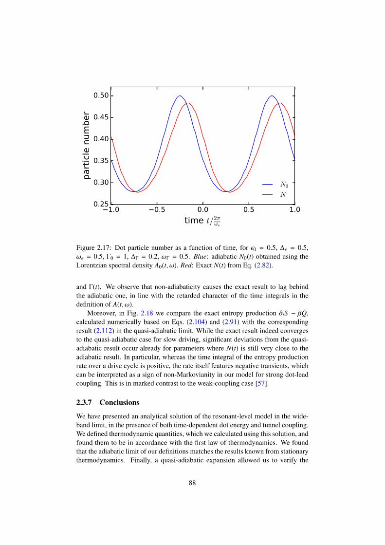
1.0 0.5 0.0 0.5 1.0
time t/2πωε
0.25
0.30
0.35
0.40
0.45
0.50part
icle
num
ber
N0
N
Figure 2.17: Dot particle number as a function of time, for ε0 = 0.5, ∆ε = 0.5,ωε = 0.5, Γ0 = 1, ∆Γ = 0.2, ωΓ = 0.5. Blue: adiabatic N0(t) obtained using theLorentzian spectral density A0(t, ω). Red: Exact N(t) from Eq. (2.82).
and Γ(t). We observe that non-adiabaticity causes the exact result to lag behindthe adiabatic one, in line with the retarded character of the time integrals in thedefinition of A(t, ω).
Moreover, in Fig. 2.18 we compare the exact entropy production ∂tS − βQ,calculated numerically based on Eqs. (2.104) and (2.91) with the correspondingresult (2.112) in the quasi-adiabatic limit. While the exact result indeed convergesto the quasi-adiabatic case for slow driving, significant deviations from the quasi-adiabatic result occur already for parameters where N(t) is still very close to theadiabatic result. In particular, whereas the time integral of the entropy productionrate over a drive cycle is positive, the rate itself features negative transients, whichcan be interpreted as a sign of non-Markovianity in our model for strong dot-leadcoupling. This is in marked contrast to the weak-coupling case [57].
2.3.7 Conclusions
We have presented an analytical solution of the resonant-level model in the wide-band limit, in the presence of both time-dependent dot energy and tunnel coupling.We defined thermodynamic quantities, which we calculated using this solution, andfound them to be in accordance with the first law of thermodynamics. We foundthat the adiabatic limit of our definitions matches the results known from stationarythermodynamics. Finally, a quasi-adiabatic expansion allowed us to verify the
88
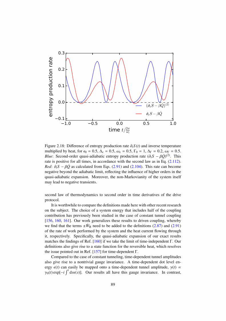
1.0 0.5 0.0 0.5 1.0
time t/2πωε
0.1
0.0
0.1
0.2
0.3entr
opy p
roduct
ion r
ate
( tS− βQ)(2)
tS− βQ
Figure 2.18: Difference of entropy production rate ∂tS (t) and inverse temperaturemultiplied by heat, for ε0 = 0.5, ∆ε = 0.5, ωε = 0.5, Γ0 = 1, ∆Γ = 0.2, ωΓ = 0.5.Blue: Second-order quasi-adiabatic entropy production rate (∂tS − βQ)(2). Thisrate is positive for all times, in accordance with the second law as in Eq. (2.112).Red: ∂tS − βQ as calculated from Eqs. (2.91) and (2.104). This rate can becomenegative beyond the adiabatic limit, reflecting the influence of higher orders in thequasi-adiabatic expansion. Moreover, the non-Markovianity of the system itselfmay lead to negative transients.
second law of thermodynamics to second order in time derivatives of the driveprotocol.
It is worthwhile to compare the definitions made here with other recent researchon the subject. The choice of a system energy that includes half of the couplingcontribution has previously been studied in the case of constant tunnel coupling[156, 160, 161]. Our work generalizes these results to driven coupling, wherebywe find that the terms ±WB need to be added to the definitions (2.87) and (2.91)of the rate of work performed by the system and the heat current flowing throughit, respectively. Specifically, the quasi-adiabatic expansion of our exact resultsmatches the findings of Ref. [160] if we take the limit of time-independent Γ. Ourdefinitions also give rise to a state function for the reversible heat, which resolvesthe issue pointed out in Ref. [157] for time-dependent Γ.
Compared to the case of constant tunneling, time-dependent tunnel amplitudesalso give rise to a nontrivial gauge invariance. A time-dependent dot level en-ergy ε(t) can easily be mapped onto a time-dependent tunnel amplitude, γ(t) ∝γ0(t) exp[−i
∫ tdsε(s)]. Our results all have this gauge invariance. In contrast,
89
several works have suggested that system quantities can be defined by isolatingε(t) dependent quantities in the “super-system” observables [160, 161]. However,this procedure is not gauge-invariant and thus cannot be used in the case of time-dependent tunnel amplitudes.
Several challenges remain to be overcome on the way to a full understanding ofnonequilibrium quantum thermodynamics in the resonant-level model: Beyond thewide-band approximation, the precise correspondence between the Green’s func-tion approach and the results obtained for the grand canonical ensemble in theadiabatic limit as in Sec. 2.3.4 is still unclear. Similar problems arise if one consid-ers higher moments of the Hamiltonian instead of expectation values only [161].Finally, it is an appealing prospect to find a version of the second law that holds forall orders in drive speed as opposed to just second order.
2.3.8 Appendix: Adiabatic limit
In the following, we derive approximations for the quantities defined in Sec. 2.3.3for the case of slow driving. First, we establish the adiabatic limit of infinitelyslow drive. Then, we move to the quasi-adiabatic case by expanding the exactexpressions in terms of time derivatives of the drive protocol [ε(t),Γ(t)].
The function
V(t, ω) =
∫ t
−∞
ds√
Γ(s)e∫ t
s dy[iω−iε(y)−Γ(y)] (2.114)
from Eq. (2.81) is the central subject of the calculations in this section. Its staticlimit is obtained by assuming constant ε ≡ ε0 and Γ ≡ Γ0,
V (0)(ω) =
√Γ0
i(ε0 − ω) + Γ0. (2.115)
Using this to calculate A(0) = 2|V (0)(ω)|2, we obtain
A(0)(ω) =2Γ0
(ω − ε0)2 + Γ20
, (2.116)
which coincides with the spectral function A0(ω). From Eq. (2.82), we immedi-ately obtain the particle number,
N(0) =
∫dω2π
A0(ω)nF(ω) =
∫dω2π
2Γ0
(ω − ε0)2 + Γ20
nF(ω). (2.117)
Similarly, we obtain for the system energy,
E(0)S =
∫dω2πωnF(ω)A0(ω), (2.118)
since the second term in Eq. (2.86) is approximated by zero.
90
2.3.9 Appendix: Quasi-adiabatic expansion
In this section, we move beyond the adiabatic limit in approximating the particlenumber, system energy, as well as heat and work rates. To this end we reinstate thetime dependence of Γ and ε in V(t, ω) which occurs in all the quantities consideredhere. We then expand both drives up to second order in time derivatives resultingin the expansion4
V (2)(t, ω) =
√Γ
i(ε − ω) + Γ−
∂tΓ
2√
Γ
1[i(ε − ω) + Γ]2 +
3√
Γ(i∂tε + ∂tΓ)2
[i(ε − ω) + Γ]5
+
[−∂tΓ(i∂tε + ∂tΓ)
4√
Γ−
16
√Γ(i∂2
t ε + ∂2t Γ)
]6
[i(ε − ω) + Γ]4
+
∂2t Γ
4√
Γ−
(∂tΓ)2
8√
Γ3+
√Γ
2(i∂tε + ∂tΓ)
2[i(ε − ω) + Γ]3 , (2.119)
where all drives are evaluated at time t. By substituting this expression, we readilyobtain second-order results for the currents ∂tN, W, ∂tES, and Q. Since the second-order contributions to these quantities go beyond the adiabatic results in the senseof Sec. 2.3.4, we refer to them as quasi-adiabatic expansion.
The particle current is given by the time derivative of Eq. (2.82).
∂tN(t) =
∫dω2π
nF(ω)∂tA(t, ω), (2.120)
where by substituting Eq. (2.119), we find the second-order expansion of ∂tA(t, ω) =
2∂t|V(t, ω)|2 to be given by
[∂tA(t, ω)](2) = (∂ΓA0∂tΓ + ∂εA0∂tε)
− ∂t∂ω
A20Γ
2∂tω − ε
Γ
, (2.121)
where we suppress the arguments t andω from here onward. Therefore, the second-order quasi-adiabatic expansion of the particle current reads
[∂tN(t)](2) =
∫dω2π
nF (∂ΓA0∂tΓ + ∂εA0∂tε)
+
∫dω2π∂ωnF∂t
A20Γ
2∂tω − ε
Γ
. (2.122)
Analogously, by starting from Eq. (2.86), we find the second-order expression forthe system energy current,
[∂tES](2) =
∫dω2πωnF (∂ΓA0∂tΓ + ∂εA0∂tε)
+
∫dω2πω∂ωnF∂t
A20Γ
2∂tω − ε
Γ
. (2.123)
4The expansion of V(t, ω) was performed by Thomas L. Schmidt.
91
The work flow into the system consists of three distinct contributions, W = WSB +
WC +WB, the first two of which require expansion: The power applied to the super-system is approximated by expanding Eq. (2.88),
W (2)SB =
∫dω2π
nFA0
(∂tε +
ω − ε
Γ∂tΓ
)−
Γ2
2
∫dω2π∂ωnFA2
0
(∂tω − ε
Γ
)2, (2.124)
and the chemical work flow is given by W(2)C = µ[∂tN](2), which is immediate from
Eq. (2.122). Finally, we consider the heat current, Q = −∂t 〈HB + HT/2〉−WC−WB.The last term is the reverse of the first-order expression quantifying mechanicalwork performed on the bath, whereas the first two terms can be expressed as as
− ∂t 〈HB + HT/2〉 − µ∂tN = −WSB + ∂tES − µ∂tN, (2.125)
which leads to the approximation
Q(2) = −W(2)SB + (∂tES)(2) − µ∂tN(2) − WB
= −
∫dω2π
nFA0
(∂tε +
ω − ε
Γ∂tΓ
)+
∫dω2π
(ω − µ)nF (∂ΓA0∂tΓ + ∂εA0∂tε)
+Γ2
2
∫dω2π∂ωnFA2
0
(∂tω − ε
Γ
)2
+
∫dω2π
(ω − µ)∂ωnF∂t
A20Γ
2∂tω − ε
Γ
− WB. (2.126)
Making use of the relations β(ω − µ)nF(ω) = σF(ω) − log(1 + e−βω
)and
∂ΓA0(ω) = −∂ω[(ω − ε)A0/Γ], we can rewrite the first-order terms as
Q(1) =1β
∫dω2πσF (∂ΓA0∂tΓ + ∂εA0∂tε)
−1β
∫dω2π
log(1 + e−βω
)∂ω
(−ω − ε
ΓA0∂tΓ − A0∂tε
)−
∫dω2π
nFA0
(ω − ε
Γ∂tΓ + ∂tε
)− WB, (2.127)
where after integrating by parts, the second line cancels the third. Furthermore,by comparing Eq. (2.127) to the time derivative of the equilibrium grand canonicalpotential of Eq. (2.97) and the work rate in Eq. (2.124) we obtain the relation(2.103).
92
2.4 Initial states in quantum thermodynamics
We examine the role of initial-state contributions to the quantum thermodynamicsof the driven resonant-level model. By solving the equations of motion, we obtainan analytical expression for the work performed on the system given a generaldrive protocol and arbitrary coupling to a bath. We establish that our definition ofwork coincides with the one introduced in stochastic thermodynamics. This con-nection is shown to imply that in the long-time limit, the work performed as a resultof a periodic drive is positive also for a non-thermal initial state, in accordancewith the second law of thermodynamics. This section was written in collaborationwith Edvin G. Idrisov, Massimilano Esposito, and Thomas L. Schmidt. It representswork in progress and will be submitted for publication in the near future.
2.4.1 Introduction
Quantum mechanics and thermodynamics are often thought of as operating onvastly different length scales. While the former is the foundation of our under-standing of physics at the nanoscale, the latter is rooted in the macroscopic world,where it is instrumental in the design of work cycles and machines. It is onlyin recent years that fabrication and measurement methods have improved to thepoint that machines on the quantum scale can be reliably implemented and ana-lyzed [97, 138, 139, 140, 37]. A theory of quantum thermodynamics – or evenjust classical microscopic thermodynamics – has thus become highly desirable, asit would facilitate goals such as the design of novel electronic components as wellthe understanding of chemical reactions, among others [166, 138, 167, 168].
The central goal of quantum thermodynamics is to adapt the laws of thermo-dynamics in order to capture the behavior of quantum systems, while preserving asmuch as possible of the generality that constitutes the power of classical thermody-namics. On the path to this goal, obstacles are manifold. Many of the underlyingpremises of classical thermodynamics do not carry over to the quantum regime.First, the thermodynamic limit of large particle numbers is clearly not given inquantum systems. Second, the smaller the systems in question are, the more atten-tion has to be paid to the precise manner of how they are coupled to each other.In particular, the thermodynamics of strongly coupled quantum systems still lacksa unifying framework, in spite of considerable recent attention [141, 90, 81, 91].Third, the roles of fluctuations and non-equilibrium, already nontrivial in classicalsystems [86, 143], are even more prominent in quantum settings.
A great variety of techniques have been employed to establish quantum ther-modynamics: The case of a system weakly coupled to a bath was resolved us-ing open systems [67, 9, 69]. The strong-coupling situation has proved to bemore complex. One promising approach is given by stochastic thermodynamics[70, 78, 80, 84, 83, 81], which has been used to give a consistent definition ofwork for non-equilibrium quantum systems as well as to establish general fluc-tuation theorems [72, 73, 74, 77]. However, the notions of system energy and
93
heat flows, and thus the first law of thermodynamics, are less straightforward inthis approach [81]. On the other hand, recent work has examined the possibil-ity of using exactly solvable model systems to define thermodynamic quantities[160, 169]. There, several sets of definitions exist that fulfill a quantum ver-sion of the first law, but a general formulation of the second law remains elusive[156, 170, 157, 158, 159, 160, 161, 162, 163, 171, 169].
In this work, we examine the role of the initial state in the quantum thermo-dynamics of the strongly coupled resonant-level model coupled to a metallic lead.Considering the work performed by a periodic driving protocol, we establish a linkto stochastic thermodynamics. There, it is known that the work production overa drive period is positive provided that the composite system of dot and lead isinitially in a thermal state, which can be seen as a signature of the second law ofthermodynamics for quantum systems. We show that, for an initially uncoupledsetup of dot and lead, the work production in the long-time limit is also positive,even though the composite system is never in a thermal state. Furthermore, weexhibit the non-equivalence of the two configurations in the long-time limit byconsidering nonlocal correlations in the lead.
Our analysis is structured as follows: In Sec. 2.4.2, we lay out the resonant-level model and give its solution in the presence of arbitrary coupling strength anddrive protocol, taking into account initial state effects. In Sec. 2.4.3, we discuss thework production as a result of a periodic driving protocol, and see that it is closelyrelated to the work production discussed in stochastic thermodynamics. Moreover,we introduce the factorized and thermal initial states whose thermodynamics aimto compare. Next, we use Sec. 2.4.4 to analyze the limit of long evolution timesand quantify the asymptotic effect of the initial configuration of the system. Inparticular, we find that the asymptotic work production per period is positive evenin situations without thermalization at any point in time. We furthermore use theevolution of correlations in the lead to point out that initial-state dependence stilloccurs in non-local correlators. A summary of our results is given in Sec. 2.4.5.
2.4.2 Model
The resonant-level model for a quantum dot has previously been solved with thenon-equilibrium Green’s function formalism [160, 169]. Here we take a differentapproach, using equations of motion [153]. The system consists of a single electronlevel coupled to metallic lead of size L, which acts as a bath. Its Hamiltonian isgiven by
H(t) = HD(t) + HB + HT(t), (2.128)
HD(t) = ε(t)d†d,
HB = −ivF
∫ ∞
−∞
dxψ†(x)∂xψ(x),
HT(t) = γ(t)d†ψ(x = 0) + h. c.,
94
where HD(t), HB, and HT(t) are the dot, lead, and coupling Hamiltonians, respec-tively. We assume a linear energy spectrum in the lead, with Fermi velocity vF.The continuum limit L → ∞ is implicit here, and is in agreement with the infiniteintegration domain in HB. The operators d and d† respectively annihilate or createan electron on the dot, and similarly ψ(x) and ψ†(x) are the annihilation and cre-ation operators of a lead particle at position x. They fulfill fermionic commutationrelations, d, d† = 1, and ψ(x), ψ†(y) = δ(x − y). We allow for a general driveprotocol, with both the dot energy ε and the tunnel coupling amplitude γ ∈ R de-pending on time. No restrictions are placed on the strength of the coupling or onthe speed of the drive. The only further approximation we use consists of takingthe wide-band limit of the dot-lead coupling, meaning a constant density of statesin the leads, ρ = 1/(2πvF). Lastly, the spin degree of freedom is not relevant to ouranalysis, so we do not consider it here.
The resulting equations of motion in the Heisenberg picture read
∂td(t) = −iε(t)d(t) − iγ(t)ψ(x = 0, t)
∂tψ(x, t) = −vF∂xψ(x, t) − iγ(t)d(t)δ(x). (2.129)
As shown in Ref. [153], these admit the solution
d(t) = e∫ t
t0ds(−iε(s)−Γ(s))d(t0)
− i∫ t
t0dsγ(s)e
∫ ts dy(−iε(y)−Γ(y))ψ0(−vF(s − t0)),
ψ(x, t) = ψ0(x − vF(t − t0)) −iγ(t)vF
θ(x)d(tx), (2.130)
using the shorthand tx = t − x/vF, and introducing the initial values d(t0) and ψ0(x)for the dot and lead operators, respectively.
This solution allows us to calculate the time evolution of any observable of thesystem. For instance, the particle number on the dot is given by
N(t) ≡⟨d†(t)d(t)
⟩= tr
[ρ(t0)d†(t)d(t)
], (2.131)
where in the second equality we introduced the initial density matrix ρ(t0) of thecomposite system of dot and lead. Moreover, we define the mechanical work rateas
W(t) ≡ 〈∂tH(t)〉 , (2.132)
in agreement with Refs. [74, 156, 160]. Here and in the following we use a dotsuperscript to indicate that a quantity is interpreted as a rate, not necessarily thatit is a time derivative [169]. Explicit expressions for N(t) and W(t) are given inApp. 2.4.6.
95
2.4.3 Work production
The definition of work is a subtle matter in quantum thermodynamics: Work can-not be defined as an observable since it is related to an energy difference and hencerequires more than one measurement [80, 88, 74]. Below, we show the equiva-lence of our definition in Eq. (2.132) and the work rate as introduced in stochasticthermodynamics.
The latter approach [80] defines the mechanical work performed on a systembetween the time of initialization t0 and a final time t as the difference between twomeasurements of the total system energy, one at t0 and the other at t. In this way,work is represented as a random variable with probability density function p(w, t).Its expectation value is given by
〈w(t)〉 = tr[U†(t, t0)H(t)U(t, t0)ρ(t0)
]− tr
[H(t0)ρ(t0)
], (2.133)
where ρ(t0) = e−βH(t0)/ tr e−βH(t0) denotes the density matrix of a thermal initialstate of the composite system, and U(t, t0) is the propagator in the Schrodingerpicture, fulfilling
i∂tU(t, t0) = H(t)U(t, t0). (2.134)
〈w(t)〉 can be shown to be bounded from below by the difference of the equilibriumfree energies calculated with the initial and final Hamiltonians [78, 84],
〈w(t)〉 ≥ F(t) − F(t0), (2.135)
where the free energy F(t) of a hypothetical equilibrium state at time t is given by
F(t) = −1β
log tr e−βH(t). (2.136)
In particular, Eq. (2.135) implies positive work production,
〈w(t)〉 ≥ 0, (2.137)
for a periodic drive protocol that ensures F(t) = F(t0).On the other hand, Eq. (2.132) implies
W(t) = tr[U†(t, t0)∂tH(t)U(t, t0)ρ(t0)
]. (2.138)
By taking the time derivative of Eq. (2.133), we see that the work rates in bothapproaches are the same,
∂t〈w(t)〉 = W(t). (2.139)
This implies that the positivity relation Eq. (2.137) also holds for the integratedwork produced according to Eq. (2.138), if the composite system is prepared in athermal initial state.
96
The prerequisite of an initially thermal state is rather restrictive: Consider adot prepared in isolation from a thermalized lead, the coupling to which is thenswitched on afterwards, together with the drive protocol. In this case, the com-posite system will never fully thermalize. Hence, the commonly required initialthermalization may be hard to achieve in practice. In the following, we use thework production to examine how the thermodynamics of a system prepared likethis differs from that of an initially thermalized system.
Specifically, we compare two initial state configurations: First, a factorizedstate (i) of the composite system, ρ(i)(t0) = ρD(t0) ⊗ ρB(t0), where the bath is in athermal state at an inverse temperature β,
ρB(t0) =e−βHB(t0)
tr e−βHB(t0) . (2.140)
We specify the initial state of the system by supplying its initial occupation N(t0).Setup (i) is analogous to the choice in Ref. [169], but with a finite initial time t0.Second, we consider a state (ii), where the composite system is thermalized as awhole,
ρ(ii)(t0) =e−βH(t0)
tr e−βH(t0) , (2.141)
which is the usual assumption in stochastic thermodynamics.As a first part of the comparison, we illustrate the evolution during the first few
drive cycles. To this end, we let each of these states evolve subject to the exampledrive protocol
ε(t) = δ1 + δ2 cos Ωt
Γ(t) = Γ0, (2.142)
choosing a sinusoidal drive of the dot energy and a constant dot-lead tunneling rateΓ0 = γ2
0/(2vF). The work rates corresponding to either of the setups can be explitlycalculated using the results in App. 2.4.6. The evolution of the work rates startingfrom the initial time are visualized in Fig. 2.19, with the asymptotic work rate W∞obtained for an initial state in the infinite past, t0 = −∞ added for comparison. Itis evident that close to t0 the effects of the initial state are significant, resulting inpositive work production for the thermalized setup (ii) over the course of a driveperiod T = 2π/Ω,
∆W (ii) ≡
∫ t0+T
t0dtW(i)
t0 ≥ 0, (2.143)
in agreement with Eq. (2.137). For the factorized setup (i) on the other hand,the integrated work production during the first drive cycle is negative. Movingaway from the initial time, the dependence of the work rate on the initial stateexponentially, and in both setups the work rate approaches the asymptotic, W∞,
97
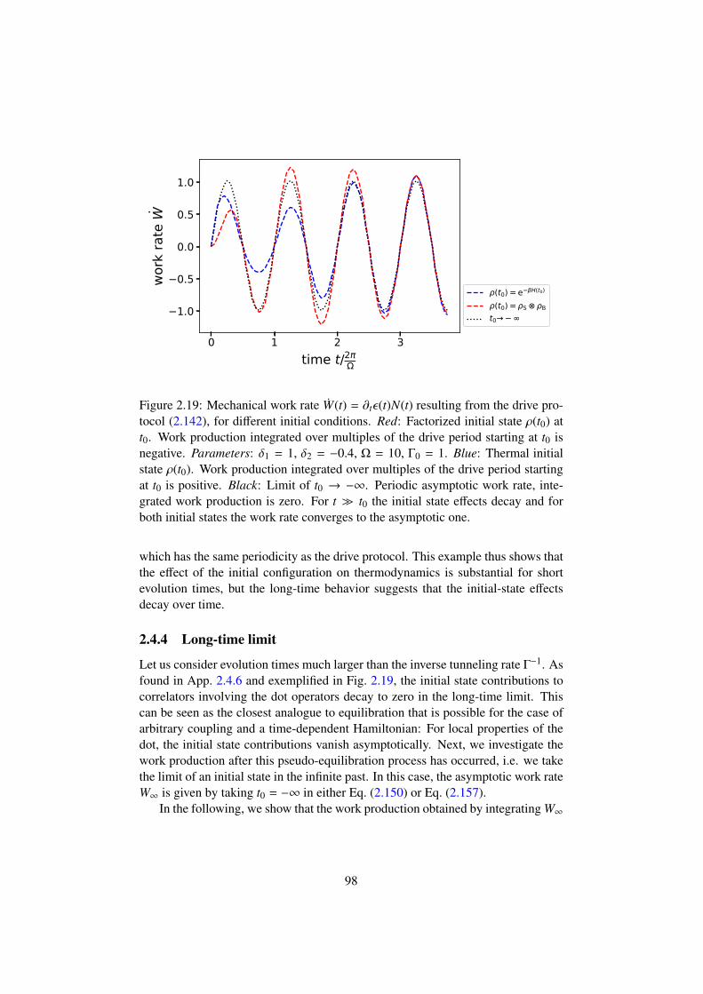
0 1 2 3time t/2
1.0
0.5
0.0
0.5
1.0
work
rate
W
(t0) = e H(t0)
(t0) = S Bt0
Figure 2.19: Mechanical work rate W(t) = ∂tε(t)N(t) resulting from the drive pro-tocol (2.142), for different initial conditions. Red: Factorized initial state ρ(t0) att0. Work production integrated over multiples of the drive period starting at t0 isnegative. Parameters: δ1 = 1, δ2 = −0.4, Ω = 10, Γ0 = 1. Blue: Thermal initialstate ρ(t0). Work production integrated over multiples of the drive period startingat t0 is positive. Black: Limit of t0 → −∞. Periodic asymptotic work rate, inte-grated work production is zero. For t t0 the initial state effects decay and forboth initial states the work rate converges to the asymptotic one.
which has the same periodicity as the drive protocol. This example thus shows thatthe effect of the initial configuration on thermodynamics is substantial for shortevolution times, but the long-time behavior suggests that the initial-state effectsdecay over time.
2.4.4 Long-time limit
Let us consider evolution times much larger than the inverse tunneling rate Γ−1. Asfound in App. 2.4.6 and exemplified in Fig. 2.19, the initial state contributions tocorrelators involving the dot operators decay to zero in the long-time limit. Thiscan be seen as the closest analogue to equilibration that is possible for the case ofarbitrary coupling and a time-dependent Hamiltonian: For local properties of thedot, the initial state contributions vanish asymptotically. Next, we investigate thework production after this pseudo-equilibration process has occurred, i.e. we takethe limit of an initial state in the infinite past. In this case, the asymptotic work rateW∞ is given by taking t0 = −∞ in either Eq. (2.150) or Eq. (2.157).
In the following, we show that the work production obtained by integrating W∞
98
over a drive period is positive far away from the initial time,
∆W∞ =
∫ T
0dtW∞(t) ≥ 0, (2.144)
which establishes an asymptotic version of Eq. (2.143). Indeed, the exponentialdecay of the initial state contributions to the work rate W(ii) calculated with thethermalized initial state implies
∆W(ii)m ≡
∫ t0+(m+1)T
t0+mTdtW(ii)(t) →
m→∞∆W∞, (2.145)
where the periodicity W∞(t) = W∞(t + T ) is used to fix the integration intervalon the right hand side to [0,T ]. If now ∆W∞ were strictly negative, Eq. (2.145)would imply that for sufficiently large m, all the increments ∆W(ii)
m are boundedfrom above by a strictly negative number. On the other hand, since W (ii) is basedon a thermalized initial state, Eq. (2.137) implies
n∑m=0
∆W (ii)m =
∫ t0+(n+1)T
t0dtW(ii)(t) ≥ 0 (2.146)
for any integer n, which leads to a contradiction. Hence we proved ∆W∞ ≥ 0.The expression for W (i) in Eq. (2.150) shows that the integrated work productionper drive cycle converges to ∆W∞ in the same manner as for W (ii). Therefore, theasymptotic work production per cycle is positive, even for a factorized initial statewith negative work production during the early drive cycles. We conclude that inthe long-time limit, the work production in our model is positive even though theconditions imposed by stochastic thermodynamics are not met.
This result does however not imply that the two initial setups (i) and (ii) leadto asymptotically equivalent evolution for all observables: The bath correlators〈ψ†(x, t)ψ(y, t)〉 do not converge in the same manner as the local quantities N(t)and W in the long-time limit. As detailed in App. 2.4.6, for any evolution time t,non-decaying initial-state signatures remain in correlators of some bath sites thatare sufficiently far away from the dot. This makes manifest the difference betweena thermal state of the composite system and an initially factorized state that is thencoupled and left to evolve.
2.4.5 Conclusion
We connected stochastic thermodynamics to a set of definitions in terms of theexpectation values in the resonant-level model for a driven quantum dot at arbitrarycoupling to a bath. In particular, the definitions of the work rate known from theliterature in both contexts are shown to coincide. This implies a positive workproduction during a drive cycle, if the system starts out in thermal equilibrium.By explicitly calculating the work rate in the resonant-level model for a thermal
99
initial state as well as for a factorized initial state of dot and leads, we see that theone-period work production is the same for both initial setups if the initial time liesin the infinite past. This is then used to show that the work production per periodin the resonant-level model in the long-time limit is also positive, even thoughthe system may not have been in a thermal state at any point, as is the case forthe factorized setup. Our results indicate that the validity of the laws of quantumthermodynamics does not rely on an initially thermalized state.
2.4.6 Appendix: Expectation values
Here, we use the solution of the Heisenberg equations,
d(t) = e∫ t
t0ds(−iε(s)−Γ(s))d(t0) − i
∫ t
t0dsγ(s)e
∫ ts dy(−iε(y)−Γ(y))ψ0(−vF(s − t0)),
ψ(x, t) = ψ0(x − vF(t − t0)) −iγ(t)vF
θ(x)d(t), (2.147)
to calculate observables for the two different initial setups (i) and (ii). Our focuslies on the dot particle number N(t) =
⟨d†(t)d(t)
⟩, the rate of mechanical work
W = 〈∂tH(t)〉, as well as on the equal-time bath correlator Cxy(t) =⟨ψ†(x, t)ψ(y, t)
⟩.
For setup (i), we use the factorized initial state
ρ(i)(t0) = ρD(t0) ⊗[e−βHB(t0)/ tr e−βHB(t0)
]. (2.148)
This leads to the initial correlators⟨d†(t0)d(t0)
⟩= trD
[ρD(t0)d†(t0)d(t0)
]≡ N(t0),⟨
d†(t0)ψ(x, t0)⟩
= 0,⟨ψ†(x, t0)ψ(y, t0)
⟩=
1vF
∫dω2π
eiω y−xvF nF(ω) (2.149)
where we denoted the initial dot occupation by N(t0) and used the wide-band limit,as well as the thermal initial occupation of the bath modes, to calculate the bathcorrelator. In order to calculate the lead correlator, we considered the momen-tum space representation ψ(x, t0) =
∑k eikxck/
√L, with the thermal expectation
value for the lead mode given by 〈c†kcq〉 = δkqnF(εk). Moreover, we took the wide-band limit of the momentum summation, which leads to the frequency integral∑
k /L → ρ∫
dω, with the density of states ρ = 1/(2πvF). The divergence of thebath correlator is due to linearizing the spectrum of the lead, εk = vFk, and can becured by imposing a cutoff. We will not explicitly perform this procedure in thefollowing. Substituting Eq. (2.147) into the desired expectation values, we can use
100
the initial correlators from Eq. (2.149) to obtain
N(i)(t) = N(t0)e−2∫ t
t0dyΓ(y)
+
∫dω2π
nF(ω)A(t, ω)
W (i)(t) = ∂tε(t)N(t) + 4∂t√
Γ(t)∫
dω2π
nF(ω) Im V(t, ω)
C(i)xy(t) =
1vF
∫dω2π
eiω y−xvF nF(ω)
+γ(tx)γ(ty)
v2F
θ(x)θ(y)N(t0)e∫ tx
t0ds[iε(s)−Γ(s)]e
∫ tyt0
ds[−iε(s)−Γ(s)]
+ 2γ(tx)γ(ty)
v2F
θ(x)θ(y)∫
dω2π
eiω y−xvF V(ty, ω)V∗(tx, ω)nF(ω)
−γ(ty)
√2vF
v2F
θ(y)∫
dω2π
eiω y−xvF V(ty, ω)nF(ω)
−γ(tx)
√2vF
v2F
θ(x)∫
dω2π
eiω y−xvF V∗(tx, ω)nF(ω), (2.150)
where, using the notation from Ref. [169], we introduced the generalized spectralfunction A(t, ω) = 2|V(t, ω)|2, with
V(t, ω) =
∫ t
t0ds
√Γ(s)e
∫ ts dy[iω−iε(y)−Γ(y)]. (2.151)
Regarding the dot quantities N(i) and W (i), we conclude that the initial conditionN(t0) only features in the first terms of N(i) and W(i), which are exponentially sup-pressed for large evolution times t − t0. Such a term will be referred to as transientin the following. As for the bath correlators C(i)
xy, we note that the first term resultsfrom the initial thermalization of the isolated bath, whereas all the others arise dur-ing the evolution in contact with the dot. These terms are hence to be understoodusing the convention γ(t) = 0 for t ≤ t0.
Given setup (ii) with ρ(ii)(t0) = e−βH(t0)
tr e−βH(t0) on the other hand, the initial thermal-ization of the composite system needs to be taken into account. More precisely, weassume the system to be in a thermal state up to the initial time t0. For all timess ≤ t0 we thus have the dot particle number⟨
d†(s)d(s)⟩
=
∫dω2π
nF(ω)A0(ω), (2.152)
the dot-lead correlator⟨d†(s)ψ(x, s)
⟩=γ0
vF
∫dω2π
eiωx/vFnF(ω)[
θ(x/vF)ω − ε0 + iΓ0
+θ(−x/vF)
ω − ε0 − iΓ0
], (2.153)
101
as well as the lead correlator⟨ψ†(x, s)ψ(y, s)
⟩=
1vF
∫dω2π
eiω y−xvF nF(ω)
− iγ2
0
v2F
∫dω2π
eiω y−xvF nF(ω)
[θ(y/vF)θ(−x/vF)ω − ε0 + iΓ0
−θ(−y/vF)θ(x/vF)ω − ε0 − iΓ0
],
(2.154)
making explicit the coupling-induced corrections to the correlators compared tothe factorized setup (i). Specifically, the diagonal dot-lead correlators 〈d†ψ0〉 donot vanish any longer, and 〈ψ†0ψ
†
0〉 acquires a correction term proportional to γ20.
a As a result of the initial thermalization, the initial dot occupation depends onthe spectral function A0(ω) = 2Γ0/[(ω − ε0)2 + Γ2
0], where ε0 and Γ0 = γ20/(2vF)
denote the initial dot energy and tunneling rate into the lead, respectively. Theinitial conditions involving the undetermined function ψ0 can be shown to followfrom Eqs. (2.152), (2.153), and (2.154):
〈d†(t0)ψ0(x)〉 =γ0
vF
∫dω2π
nF(ω)eiωx/vF
ω − ε0 − iΓ0, (2.155)
as well as
〈ψ†0(x)ψ0(y)〉 =1vF
∫dω2π
eiω y−xvF nF(ω). (2.156)
Thermalization thus manifests in the dot particle number and work rate as follows,
N(ii)(t) = e−2∫ t
t0dyΓ(y)
∫dω2π
A0(ω)nF(ω)
− iγ0
vF
√2vFe
∫ tt0
dy(iε(y)−Γ(y))∫
dω2π
e−iω(t−t0)V(t, ω)ω − ε0 − iΓ0
nF(ω)
+ iγ0
vF
√2vFe
∫ tt0
dy(−iε(y)−Γ(y))∫
dω2π
eiω(t−t0)V∗(t, ω)ω − ε0 + iΓ0
nF(ω)
+
∫dω2π
A(t, ω)nF(ω),
W (ii)(t) = ∂tε(t)N(t) + 4∂t√
Γ(t)∫
dω2π
nF(ω) Im V(t, ω)
+ 2∂tγ(t)γ0
vFRe
[e∫ t
t0dy[iε(y)−Γ(y)]
∫dω2π
nF(ω)e−iω(t−t0)
ω − ε0 − iΓ
]. (2.157)
As in the findings (2.150) for setup (i), we see that the effect of the initial thermal-ization of the composite system on the local quantities N(ii) and W (ii) consists oftransient contributions only: In the limit of t0 = −∞, the signatures of the respec-tive initial states vanish. The situation is different for the lead correlator, whichfulfills
Cxy(t) =⟨ψ†0(x − vF(t − t0))ψ0(y − vF(t − t0))
⟩+
iγ(tx)vF
θ(x)〈d†(tx)ψ(y − x, tx)〉 −iγ(ty)
vFθ(y)〈ψ†(x − y, ty)d(ty)〉 (2.158)
102
at all times t. In particular, for any t > t0, we can consider sites x, y > vF(t − t0),recalling that we took the limit of infinite lead length. For this choice, the retardedtimes tx and ty lie further in the past than t0. Hence C(ii)
xy (t) is given by the thermalcorrelator defined by the initial conditions in Eqs. (2.153) and (2.154): The sites xand y lie outside of the light cone defined by the Fermi velocity of the lead and noinformation about the drive protocol has yet reached them at time t. This impliesthat for any time t, the thermal correlations of the initial state are manifest in a non-transient manner in the lead. Inside this light cone, the lead correlator is influencedby the drive, as described by
C(ii)xy (t) =
∫dω2π
nF(ω)
1vF
eiω y−xvF
+ iγ0
vF
γ(tx)vF
θ(x)e∫ tx
t0dz(iε(z)−Γ(z)) eiω(y/vF−(t−t0))
ω − ε0 − iΓ0
−
√2vF
γ(tx)vF
θ(x)V∗(tx, ω)eiω y−xvF
− iγ0
vF
γ(ty)vF
θ(y)e∫ ty
t0dz(−iε(z)−Γ(z)) e−iω(y/vF−(t−t0))
ω − ε0 + iΓ0
−
√2vF
γ(ty)vF
θ(y)V(ty, ω)eiω y−xvF
+γ(tx)γ(ty)
v2F
θ(x)θ(y)e∫ tx
t0dz(iε(z)−Γ(z))e
∫ tyt0
dz(−iε(z)−Γ(z))A0(ω)
− i
√2vF
γ0
vF
γ(tx)γ(ty)
v2F
θ(x)θ(y)e∫ tx
t0dz(iε(z)−Γ(z))V(ty, ω)
eiω(y/vF−(t−t0))
ω − ε0 − iΓ0
+ i
√2vF
γ0
vF
γ(tx)γ(ty)
v2F
θ(x)θ(y)e∫ ty
t0dz(−iε(z)−Γ(z))V∗(tx, ω)
e−iω(x/vF−(t−t0))
ω − ε0 + iΓ0
+ 2γ(tx)γ(ty)
v2F
θ(x)θ(y)V∗(tx, ω)V(ty, ω)eiω y−xvF
. (2.159)
103

Chapter 3
Summary
Nonequilibrium quantum transport is a vast and rapidly evolving field. The workpresented in this thesis has approached the topic from multiple directions, studyingelectromechanical interaction, quantum pumping and quantum thermodynamics.These approaches, connected by the quest to understand the effects of periodicdriving on transport, have uncovered several new results:
First, in Sec. 2.1, a model for a quantum dot with strong electromechanical in-teraction was examined, coupled to a pair of leads and with a time-dependent drivecontrolling the dot energy. Without the drive, such a system is characterized byan exponential suppression of conductance due to electron-vibron interaction. Byapplying the nonequilibrium Green’s function (NEGF) formalism in conjunctionwith the polaron tunneling approximation, it was shown that this suppression oftransport can be exponentially lifted by applying a resonant drive to the dot energy.Thus, a DC current amplification may be achieved by applying an AC signal tothe quantum dot. These results are in agreement with the outcome a Born-Markovanalysis of the system.
Second, in Sec. 2.2, the same system was studied under the influence of amulti-drive protocol, introducing a time dependence in both the dot energy andin the coupling to the leads. The NEGF approach was combined with a Floquetexpansion to study charge transport through the dot under the influence of a generaldrive in the absence of bias, leading to the discovery of a protocol that can pumpa charge current in either direction, which also enjoys the exponential lifting effectdocumented in Sec. 2.1.
Third, in Sec. 2.3, a proposal for quantum thermodynamics was given for theresonant-level model of a quantum dot, allowing for strong system-bath couplingand driven system energy as well as driven coupling. The NEGF formalism is usedto obtain an analytical solution of the system dynamics for arbitrary driving speeds,which is then used to define the notions of system energy, heat, work and entropy.In doing so, the quantities are split into system and bath components in such away that they agree with the outcome of an approach using a potential of meanforce. The system quantities are shown to fulfill the first law of thermodynamics
104
as a result of energy conservation, and the second law for rates in quasi-adiabaticexpansion.
Finally, in Sec. 2.4, the influence of the initial state on quantum thermodynam-ics was studied, again using the resonant-level model as a template. After solvingthe equations of motion in the presence of an arbitrary driving protocol, thermody-namic quantities are established for both a factorized and a thermalized initial stateof dot and lead. For a thermal initial state, the theory of stochastic thermodynamicsapplies, which guarantees the positivity of the mechanical work performed by a pe-riodic drive, in accordance with the second law of thermodynamics. By comparingthe analytical expressions for the work production in the resonant-level model, itwas proven that this property is also exhibited by the asymptotics of a system thatstarts out in a factorized state and thus is never in a thermal state. Furthermore,the asymptotic properties of the dot are shown not to depend on the initial state,whereas on the other hand the correlators in the lead carry may non-transient sig-natures of the initial state, thus quantifying the non-equivalence of the two setups.
The results documented here show that the interplay of drive and nanoelec-tromechanics holds rich possibilities for further investigation and applications: Byimplementing the drive mechanism, for example via gate voltages in carbon nan-otube quantum dots, it could be examined how the lifting of Franck-Condon block-ade can be used in practice. Furthermore, our findings are not limited to carbonnanotubes, but also apply to other quantum dot architectures featuring strong elec-tromechanical coupling. Different simulation techniques may be used to studysystems beyond the paradigmatic models considered in this thesis, such as multi-dot architectures or molecular quantum dots with a complex vibrational spectrum.Work along these lines may help to identify those setups where the current responseis strongest and examine the possibility of AC-gated transistors. Lastly, it wouldbe worthwhile to consider analogous systems in the context of optomechanics andcavity quantum electrodynamics, which also involve photon degrees of freedom,opening up further further possibilities, such as the design of high-precision sen-sors.
An all-encompassing theory of nonequilibrium quantum thermodynamics isstill far off at this point, with several issues requiring further conceptual develop-ment. The incremental progress achieved in this thesis serves to consolidate someof the approaches, by using tools from transport theory to establish the laws of ther-modynamics in a model system, as well as using synergies between this approachand stochastic thermodynamics to study the long-time limit in quantum thermo-dynamics. This regime offers insight into questions of thermalization and couldserve to establish a degree of universality among initial configurations of a sys-tem. The full thermodynamic significance of the initial state is yet to be mappedout, especially with regard to entanglement and long-range correlation in the initialconfigurations. Evidently, the resonant-level model offers an accessible platform toexamine these questions without having to tackle the extraneous complexity inher-ent in other models and it is consequently far from outliving its usefulness: Bathcorrelators of the type studied in Sec. 2.4 can be used to obtain further quantita-
105
tive insight into possible nonequilibrium analogues of thermalization, and may alsobe used to study various definitions of entropy, with the possibility of easy com-parisons with the notion of “system entropy” from Sec. 2.3. The resonant-levelmodel furthermore holds potential for generalization: Once the thermodynamicsof a single level are understood, the question of an extension to multiple levelsarises naturally. Aside from the obvious appeal of describing larger systems, suchan extension would also allow to use a reaction-coordinate approach for the treat-ment of strongly coupled dots. In a similar vein, a way to explicitly account formany-body interaction is sure to be a goal of future research.
106
Bibliography
[1] M. Planck, “Zur Theorie der Warmestrahlung,” Annalen der Physik,vol. 336, no. 4, pp. 758–768, 1910.
[2] J. Park, A. N. Pasupathy, J. I. Goldsmith, C. Chang, et al., “Coulombblockade and the Kondo effect in single-atom transistors,” Nature, vol. 417,no. 6890, p. 722, 2002.
[3] S. Carnot, “Reflexions sur la puissance motrice du feu et sur les machinespropres a developper cette puissance,” Annales scientifiques de l’Ecole nor-male, 1872.
[4] C. E. Shannon, “Communication theory of secrecy systems,” Bell systemtechnical journal, vol. 28, no. 4, pp. 656–715, 1949.
[5] R. Landauer, “Irreversibility and heat generation in the computing process,”IBM journal of research and development, vol. 5, no. 3, pp. 183–191, 1961.
[6] J. Lin, “Divergence measures based on the Shannon entropy,” IEEE Trans-actions on Information theory, vol. 37, no. 1, pp. 145–151, 1991.
[7] T. J. Seebeck, Magnetische Polarisation der Metalle und Erze durchTemperatur-Differenz. No. 70, W. Engelmann, 1895.
[8] J. E. Geusic, E. O. Schulz-DuBios, and H. E. D. Scovil, “Quantum equiva-lent of the Carnot cycle,” Phys. Rev., vol. 156, pp. 343–351, Apr 1967.
[9] R. Alicki, “The quantum open system as a model of the heat engine,” Jour-nal of Physics A: Mathematical and General, vol. 12, no. 5, p. L103, 1979.
[10] Y. Shirasaki, G. J. Supran, M. G. Bawendi, and V. Bulovic, “Emergenceof colloidal quantum-dot light-emitting technologies,” Nature Photonics,vol. 7, no. 1, p. 13, 2013.
[11] X. Michalet, F. Pinaud, L. Bentolila, J. Tsay, S. Doose, J. Li, G. Sundaresan,A. Wu, S. Gambhir, and S. Weiss, “Quantum dots for live cells, in vivoimaging, and diagnostics,” Science, vol. 307, no. 5709, pp. 538–544, 2005.
107
[12] D. Loss and D. P. DiVincenzo, “Quantum computation with quantum dots,”Phys. Rev. A, vol. 57, pp. 120–126, Jan 1998.
[13] S. W. Koch et al., Semiconductor quantum dots, vol. 2. World Scientific,1993.
[14] A. P. Alivisatos, “Semiconductor clusters, nanocrystals, and quantum dots,”Science, vol. 271, no. 5251, pp. 933–937, 1996.
[15] J. M. Thijssen and H. S. J. Van der Zant, “Charge transport and single-electron effects in nanoscale systems,” physica status solidi (b), vol. 245,no. 8, pp. 1455–1470, 2008.
[16] S. Datta, Quantum transport: atom to transistor. Cambridge universitypress, 2005.
[17] C. W. J. Beenakker, “Theory of Coulomb-blockade oscillations in the con-ductance of a quantum dot,” Phys. Rev. B, vol. 44, pp. 1646–1656, Jul 1991.
[18] H. Grabert and M. H. Devoret, Single charge tunneling: Coulomb block-ade phenomena in nanostructures, vol. 294. Springer Science & BusinessMedia, 2013.
[19] Y. Alhassid, “The statistical theory of quantum dots,” Rev. Mod. Phys.,vol. 72, pp. 895–968, Oct 2000.
[20] J. Koch, F. von Oppen, Y. Oreg, and E. Sela, “Thermopower of single-molecule devices,” Phys. Rev. B, vol. 70, p. 195107, Nov 2004.
[21] J. Koch and F. von Oppen, “Franck-Condon blockade and giant Fano factorsin transport through single molecules,” Phys. Rev. Lett., vol. 94, p. 206804,May 2005.
[22] A. Pasupathy, J. Park, C. Chang, A. Soldatov, S. Lebedkin, R. Bialczak,J. Grose, L. Donev, J. Sethna, D. Ralph, et al., “Vibration-assisted electrontunneling in C140 transistors,” Nano Letters, vol. 5, no. 2, pp. 203–207,2005.
[23] J. Koch, F. von Oppen, and A. V. Andreev, “Theory of the Franck-Condonblockade regime,” Phys. Rev. B, vol. 74, p. 205438, Nov 2006.
[24] S. Ilani and P. L. McEuen, “Electron transport in carbon nanotubes,” AnnualReview of Condensed Matter Physics, vol. 1, no. 1, pp. 1–25, 2010.
[25] E. A. Laird, F. Kuemmeth, G. A. Steele, K. Grove-Rasmussen, J. Nygård,K. Flensberg, and L. P. Kouwenhoven, “Quantum transport in carbon nan-otubes,” Rev. Mod. Phys., vol. 87, pp. 703–764, Jul 2015.
108
[26] A. Benyamini, A. Hamo, S. V. Kusminskiy, F. von Oppen, and S. Ilani,“Real-space tailoring of the electron-phonon coupling in ultraclean nan-otube mechanical resonators,” Nature Physics, vol. 10, no. 2, pp. 151–156,2014.
[27] H. G. Craighead, “Nanoelectromechanical systems,” Science, vol. 290,no. 5496, pp. 1532–1535, 2000.
[28] C. S. Lau, H. Sadeghi, G. Rogers, S. Sangtarash, P. Dallas, K. Porfyrakis,J. Warner, C. J. Lambert, G. A. D. Briggs, and J. A. Mol, “Redox-dependentFranck-Condon blockade and avalanche transport in a graphene-fullerenesingle-molecule transistor,” Nano letters, vol. 16, no. 1, pp. 170–176, 2015.
[29] E. Burzuri, Y. Yamamoto, M. Warnock, X. Zhong, K. Park, A. Cornia, andH. S. J. van der Zant, “Franck–Condon blockade in a single-molecule tran-sistor,” Nano Letters, vol. 14, no. 6, pp. 3191–3196, 2014.
[30] R. Leturcq, C. Stampfer, K. Inderbitzin, L. Durrer, C. Hierold, E. Mariani,M. G. Schultz, F. von Oppen, and K. Ensslin, “Franck-Condon blockade insuspended carbon nanotube quantum dots,” Nature Physics, vol. 5, no. 5,pp. 327–331, 2009.
[31] K. Flensberg, “Electron–vibron coupling in suspended nanotubes,” NewJournal of Physics, vol. 8, no. 1, p. 5, 2006.
[32] W. Izumida and M. Grifoni, “Phonon-assisted tunnelling in interacting sus-pended single-wall carbon nanotubes,” New Journal of Physics, vol. 7, no. 1,p. 244, 2005.
[33] E. Mariani and F. von Oppen, “Electron-vibron coupling in suspended car-bon nanotube quantum dots,” Phys. Rev. B, vol. 80, p. 155411, Oct 2009.
[34] R.-P. Riwar and T. L. Schmidt, “Transient dynamics of a molecular quantumdot with a vibrational degree of freedom,” Phys. Rev. B, vol. 80, p. 125109,2009.
[35] S. Maier, T. L. Schmidt, and A. Komnik, “Charge transfer statistics of amolecular quantum dot with strong electron-phonon interaction,” Phys. Rev.B, vol. 83, p. 085401, Feb 2011.
[36] M. Esposito, R. Kawai, K. Lindenberg, and C. Van den Broeck, “Efficiencyat maximum power of low-dissipation Carnot engines,” Phys. Rev. Lett.,vol. 105, p. 150603, Oct 2010.
[37] M. Josefsson, A. Svilans, A. M. Burke, E. A. Hoffmann, S. Fahlvik, C. The-lander, M. Leijnse, and H. Linke, “A quantum-dot heat engine operat-ing close to the thermodynamic efficiency limits,” Nature Nanotechnology,2018.
109
[38] A. V. Feshchenko, J. V. Koski, and J. P. Pekola, “Experimental realizationof a Coulomb blockade refrigerator,” Phys. Rev. B, vol. 90, p. 201407, Nov2014.
[39] A. Svilans, M. Leijnse, and H. Linke, “Experiments on the thermoelectricproperties of quantum dots,” Comptes Rendus Physique, vol. 17, no. 10,pp. 1096–1108, 2016.
[40] H. Bruus and K. Flensberg, Many-body quantum theory in condensed matterphysics: an introduction. Oxford University Press, 2004.
[41] L. V. Keldysh et al., “Diagram technique for nonequilibrium processes,” Sov.Phys. JETP, vol. 20, no. 4, pp. 1018–1026, 1965.
[42] P. I. Arseev, “On the nonequilibrium diagram technique: derivation, somefeatures, and applications,” Physics-Uspekhi, vol. 58, no. 12, p. 1159, 2015.
[43] J. Rammer, Quantum field theory of non-equilibrium states. CambridgeUniversity Press, 2007.
[44] H. Haug and A.-P. Jauho, Quantum kinetics in transport and optics of semi-conductors, vol. 2. Springer, 2008.
[45] G. D. Mahan, Many-particle physics. Springer Science & Business Media,2013.
[46] D. C. Langreth and P. Nordlander, “Derivation of a master equation forcharge-transfer processes in atom-surface collisions,” Phys. Rev. B, vol. 43,pp. 2541–2557, Feb 1991.
[47] A.-P. Jauho, N. S. Wingreen, and Y. Meir, “Time-dependent transport ininteracting and noninteracting resonant-tunneling systems,” Phys. Rev. B,vol. 50, pp. 5528–5544, Aug 1994.
[48] Y. Meir and N. S. Wingreen, “Landauer formula for the current through aninteracting electron region,” Phys. Rev. Lett., vol. 68, pp. 2512–2515, Apr1992.
[49] C. Verzijl, J. Seldenthuis, and J. Thijssen, “Applicability of the wide-bandlimit in DFT-based molecular transport calculations,” The Journal of chem-ical physics, vol. 138, no. 9, p. 094102, 2013.
[50] T. Dittrich, P. Hanggi, G.-L. Ingold, B. Kramer, G. Schon, and W. Zwerger,Quantum transport and dissipation, vol. 3. Wiley-Vch Weinheim, 1998.
[51] M. Grifoni and P. Hanggi, “Driven quantum tunneling,” Physics Reports,vol. 304, no. 5-6, pp. 229–354, 1998.
110
[52] N. Goldman and J. Dalibard, “Periodically driven quantum systems: Ef-fective hamiltonians and engineered gauge fields,” Phys. Rev. X, vol. 4,p. 031027, Aug 2014.
[53] G. Floquet, “Sur les equations differentielles lineaires,” Ann. ENS [2],vol. 12, no. 1883, pp. 47–88, 1883.
[54] G. Teschl, Ordinary differential equations and dynamical systems, vol. 140.American Mathematical Soc., 2012.
[55] N. Tsuji, T. Oka, and H. Aoki, “Correlated electron systems periodicallydriven out of equilibrium: Floquet + DMFT formalism,” Phys. Rev. B,vol. 78, p. 235124, Dec 2008.
[56] A. Rivas and S. F. Huelga, Open Quantum Systems. Springer, 2012.
[57] H.-P. Breuer and F. Petruccione, The theory of open quantum systems. Ox-ford University Press, 2002.
[58] G. Schaller, Open quantum systems far from equilibrium, vol. 881. Springer,2014.
[59] G. Lindblad, “On the generators of quantum dynamical semigroups,”Comm. Math. Phys., vol. 48, no. 2, pp. 119–130, 1976.
[60] W.-M. Zhang, P.-Y. Lo, H.-N. Xiong, M. W.-Y. Tu, and F. Nori, “Gen-eral non-Markovian dynamics of open quantum systems,” Phys. Rev. Lett.,vol. 109, p. 170402, Oct 2012.
[61] A. Rivas, S. F. Huelga, and M. B. Plenio, “Quantum non-Markovianity:characterization, quantification and detection,” Reports on Progress inPhysics, vol. 77, no. 9, p. 094001, 2014.
[62] L. Li, M. J. Hall, and H. M. Wiseman, “Concepts of quantum non-markovianity: A hierarchy,” Physics Reports, 2018.
[63] D. M. Carberry, J. C. Reid, G. M. Wang, E. M. Sevick, D. J. Searles, andD. J. Evans, “Fluctuations and irreversibility: An experimental demonstra-tion of a second-law-like theorem using a colloidal particle held in an opticaltrap,” Phys. Rev. Lett., vol. 92, p. 140601, Apr 2004.
[64] V. Blickle, T. Speck, L. Helden, U. Seifert, and C. Bechinger, “Thermody-namics of a colloidal particle in a time-dependent nonharmonic potential,”Phys. Rev. Lett., vol. 96, p. 070603, Feb 2006.
[65] J. V. Koski, V. F. Maisi, J. P. Pekola, and D. V. Averin, “Experimental re-alization of a szilard engine with a single electron,” Proceedings of the Na-tional Academy of Sciences, vol. 111, no. 38, pp. 13786–13789, 2014.
111
[66] F. Schwabl, Statistical Mechanics. Springer, 2006.
[67] H. Spohn and J. L. Lebowitz, “Irreversible thermodynamics for quantumsystems weakly coupled to thermal reservoirs,” Adv. Chem. Phys, vol. 38,pp. 109–142, 1978.
[68] H. Spohn, “Entropy production for quantum dynamical semigroups,” Jour-nal of Mathematical Physics, vol. 19, no. 5, pp. 1227–1230, 1978.
[69] R. Kosloff, “Quantum thermodynamics: A dynamical viewpoint,” Entropy,vol. 15, no. 6, pp. 2100–2128, 2013.
[70] C. Jarzynski, “Nonequilibrium equality for free energy differences,” Phys.Rev. Lett., vol. 78, pp. 2690–2693, Apr 1997.
[71] C. B. P. Finn, Thermal Physics. Chapman & Hall, 1993.
[72] G. E. Crooks, “Entropy production fluctuation theorem and the nonequi-librium work relation for free energy differences,” Phys. Rev. E, vol. 60,pp. 2721–2726, Sep 1999.
[73] M. Esposito, U. Harbola, and S. Mukamel, “Nonequilibrium fluctuations,fluctuation theorems, and counting statistics in quantum systems,” Rev. Mod.Phys., vol. 81, pp. 1665–1702, Dec 2009.
[74] M. Campisi, P. Hanggi, and P. Talkner, “Quantum fluctuation relations:Foundations and applications,” Rev. Mod. Phys., vol. 83, pp. 771–791, Jul2011.
[75] U. Seifert, “Stochastic thermodynamics, fluctuation theorems and molecularmachines,” Reports on Progress in Physics, vol. 75, no. 12, p. 126001, 2012.
[76] G. Watanabe, B. P. Venkatesh, P. Talkner, M. Campisi, and P. Hanggi,“Quantum fluctuation theorems and generalized measurements during theforce protocol,” Phys. Rev. E, vol. 89, p. 032114, Mar 2014.
[77] J. Åberg, “Fully quantum fluctuation theorems,” Phys. Rev. X, vol. 8,p. 011019, Feb 2018.
[78] H. Tasaki, “Jarzynski relations for quantum systems and some applications,”arXiv preprint cond-mat/0009244, 2000.
[79] J. Kurchan, “A quantum fluctuation theorem,” arXiv preprint cond-mat/0007360, 2000.
[80] P. Talkner, E. Lutz, and P. Hanggi, “Fluctuation theorems: Work is not anobservable,” Phys. Rev. E, vol. 75, p. 050102, May 2007.
[81] P. Talkner and P. Hanggi, “Open system trajectories specify fluctuating workbut not heat,” Physical Review E, vol. 94, no. 2, p. 022143, 2016.
112
[82] P. Talkner and P. Hanggi, “Aspects of quantum work,” Phys. Rev. E, vol. 93,p. 022131, Feb 2016.
[83] P. Talkner, P. Hanggi, and M. Morillo, “Microcanonical quantum fluctuationtheorems,” Phys. Rev. E, vol. 77, p. 051131, May 2008.
[84] P. Talkner and P. Hanggi, “The Tasaki-Crooks quantum fluctuation theo-rem,” Journal of Physics A: Mathematical and Theoretical, vol. 40, no. 26,p. F569, 2007.
[85] C. Jarzynski, “Nonequilibrium work theorem for a system strongly coupledto a thermal environment,” Journal of Statistical Mechanics: Theory andExperiment, vol. 2004, no. 09, p. P09005, 2004.
[86] C. Jarzynski, “Stochastic and macroscopic thermodynamics of strongly cou-pled systems,” Phys. Rev. X, vol. 7, p. 011008, Jan 2017.
[87] M. F. Gelin and M. Thoss, “Thermodynamics of a subensemble of a canon-ical ensemble,” Phys. Rev. E, vol. 79, p. 051121, May 2009.
[88] M. Campisi, P. Talkner, and P. Hanggi, “Fluctuation theorem for arbitraryopen quantum systems,” Phys. Rev. Lett., vol. 102, p. 210401, May 2009.
[89] B. Roux and T. Simonson, “Implicit solvent models,” Biophysical chemistry,vol. 78, no. 1-2, pp. 1–20, 1999.
[90] U. Seifert, “First and second law of thermodynamics at strong coupling,”Phys. Rev. Lett., vol. 116, p. 020601, Jan 2016.
[91] J.-T. Hsiang and B.-L. Hu, “Quantum thermodynamics at strong coupling:Operator thermodynamic functions and relations,” Entropy, vol. 20, p. 423,2018.
[92] J. Reichert, R. Ochs, D. Beckmann, H. B. Weber, M. Mayor, and H. v.Lohneysen, “Driving current through single organic molecules,” Phys. Rev.Lett., vol. 88, p. 176804, Apr 2002.
[93] J. Park, A. N. Pasupathy, J. I. Goldsmith, C. Chang, Y. Yaish, J. R. Petta,M. Rinkoski, J. P. Sethna, H. D. Abruna, P. L. McEuen, et al., “Coulombblockade and the Kondo effect in single-atom transistors,” Nature, vol. 417,no. 6890, p. 722, 2002.
[94] W. Liang, M. Shores, M. Bockrath, J. Long, and H. Park, “Kondo resonancein a single-molecule transistor,” Nature, vol. 417, p. 725, 2002.
[95] N. Tao, “Electron transport in molecular junctions,” Nature nanotechnology,vol. 1, no. 3, pp. 173–181, 2006.
113
[96] A. Wallraff, D. I. Schuster, A. Blais, L. Frunzio, R.-S. Huang, J. Majer,S. Kumar, S. M. Girvin, and R. J. Schoelkopf, “Strong coupling of a singlephoton to a superconducting qubit using circuit quantum electrodynamics,”Nature, vol. 431, no. 7005, pp. 162–167, 2004.
[97] M. Poot and H. S. van der Zant, “Mechanical systems in the quantumregime,” Physics Reports, vol. 511, no. 5, pp. 273 – 335, 2012. Mechan-ical systems in the quantum regime.
[98] T. Frey, P. J. Leek, M. Beck, A. Blais, T. Ihn, K. Ensslin, and A. Wallraff,“Dipole coupling of a double quantum dot to a microwave resonator,” Phys.Rev. Lett., vol. 108, p. 046807, Jan 2012.
[99] Z.-L. Xiang, S. Ashhab, J. Q. You, and F. Nori, “Hybrid quantum cir-cuits: Superconducting circuits interacting with other quantum systems,”Rev. Mod. Phys., vol. 85, pp. 623–653, Apr 2013.
[100] A. K. Huttel, G. A. Steele, B. Witkamp, M. Poot, L. P. Kouwenhoven, andH. S. J. van der Zant, “Carbon nanotubes as ultrahigh quality factor mechan-ical resonators,” Nano Letters, vol. 9, no. 7, pp. 2547–2552, 2009.
[101] A. K. Huttel, H. B. Meerwaldt, G. A. Steele, M. Poot, B. Witkamp, L. P.Kouwenhoven, and H. S. J. van der Zant, “Single electron tunnelling throughhigh-q single-wall carbon nanotube NEMS resonators,” physica status solidi(b), vol. 247, no. 11-12, pp. 2974–2979, 2010.
[102] J. Chaste, M. Sledzinska, M. Zdrojek, J. Moser, and A. Bachtold,“High-frequency nanotube mechanical resonators,” Applied Physics Letters,vol. 99, no. 21, p. 213502, 2011.
[103] S. Sapmaz, P. Jarillo-Herrero, Y. M. Blanter, C. Dekker, and H. S. J. van derZant, “Tunneling in suspended carbon nanotubes assisted by longitudinalphonons,” Phys. Rev. Lett., vol. 96, p. 026801, Jan 2006.
[104] G. A. Steele, A. K. Huttel, B. Witkamp, M. Poot, H. B. Meerwaldt, L. P.Kouwenhoven, and H. S. J. van der Zant, “Strong coupling between single-electron tunneling and nanomechanical motion,” Science, vol. 325, no. 5944,pp. 1103–1107, 2009.
[105] B. Lassagne, Y. Tarakanov, J. Kinaret, D. Garcia-Sanchez, and A. Bachtold,“Coupling mechanics to charge transport in carbon nanotube mechanicalresonators,” Science, vol. 325, no. 5944, pp. 1107–1110, 2009.
[106] V. Sazonova, Y. Yaish, H. Ustunel, D. Roundy, T. A. Arias, and P. L.McEuen, “A tunable carbon nanotube electromechanical oscillator,” Nature,2004.
114
[107] J. Paaske and K. Flensberg, “Vibrational sidebands and the Kondo effect inmolecular transistors,” Phys. Rev. Lett., vol. 94, p. 176801, May 2005.
[108] I. Lang and Y. A. Firsov, “Kinetic theory of semiconductors with low mo-bility,” Sov. Phys. JETP, vol. 16, no. 5, p. 1301, 1963.
[109] T. L. Schmidt and A. Komnik, “Charge transfer statistics of a molecularquantum dot with a vibrational degree of freedom,” Phys. Rev. B, vol. 80,p. 041307, Jul 2009.
[110] G. Tang, L. Zhang, and J. Wang, “Thermal rectification in a double quantumdots system with a polaron effect,” Phys. Rev. B, vol. 97, p. 224311, Jun2018.
[111] R. Seoane Souto, A. L. Yeyati, A. Martın-Rodero, and R. C. Monreal,“Dressed tunneling approximation for electronic transport through molec-ular transistors,” Phys. Rev. B, vol. 89, p. 085412, Feb 2014.
[112] K. F. Albrecht, A. Martin-Rodero, R. C. Monreal, L. Muhlbacher, andA. Levy Yeyati, “Long transient dynamics in the Anderson-Holstein modelout of equilibrium,” Phys. Rev. B, vol. 87, p. 085127, Feb 2013.
[113] C. Timm, “Tunneling through molecules and quantum dots: Master-equation approaches,” Phys. Rev. B, vol. 77, p. 195416, May 2008.
[114] T. Krause, T. Brandes, M. Esposito, and G. Schaller, “Thermodynamics ofthe polaron master equation at finite bias,” The Journal of Chemical Physics,vol. 142, no. 13, 2015.
[115] G. Schaller, T. Krause, T. Brandes, and M. Esposito, “Single-electron tran-sistor strongly coupled to vibrations: counting statistics and fluctuation the-orem,” New Journal of Physics, vol. 15, no. 3, p. 033032, 2013.
[116] M. R. Bazrafkan and M. Ashrafi, “A driven damped harmonic oscillator inthe ket-vector representation of the density operator,” Journal of RussianLaser Research, vol. 34, no. 1, pp. 41–49, 2013.
[117] Y.-Y. Liu, K. D. Petersson, J. Stehlik, J. M. Taylor, and J. R. Petta, “Pho-ton emission from a cavity-coupled double quantum dot,” Phys. Rev. Lett.,vol. 113, p. 036801, Jul 2014.
[118] J. J. Viennot, M. C. Dartiailh, A. Cottet, and T. Kontos, “Coherent couplingof a single spin to microwave cavity photons,” Science, vol. 349, no. 6246,pp. 408–411, 2015.
[119] H. Pothier, P. Lafarge, C. Urbina, D. Esteve, and M. H. Devoret, “Single-electron pump based on charging effects,” EPL (Europhysics Letters),vol. 17, no. 3, p. 249, 1992.
115
[120] M. Switkes, C. Marcus, K. Campman, and A. Gossard, “An adiabatic quan-tum electron pump,” Science, vol. 283, no. 5409, pp. 1905–1908, 1999.
[121] M. V. Moskalets, Scattering matrix approach to non-stationary quantumtransport. World Scientific, 2011.
[122] P. San-Jose, E. Prada, S. Kohler, and H. Schomerus, “Single-parameterpumping in graphene,” Phys. Rev. B, vol. 84, p. 155408, Oct 2011.
[123] L. E. F. F. Torres, H. L. Calvo, C. G. Rocha, and G. Cuniberti, “Enhancingsingle-parameter quantum charge pumping in carbon-based devices,” Ap-plied Physics Letters, vol. 99, no. 9, p. 092102, 2011.
[124] D. Fioretto and A. Silva, “Phase coherence, inelastic scattering, and in-teraction corrections in pumping through quantum dots,” Phys. Rev. Lett.,vol. 100, p. 236803, Jun 2008.
[125] E. Prada, P. San-Jose, and H. Schomerus, “Quantum pumping in graphene,”Phys. Rev. B, vol. 80, p. 245414, Dec 2009.
[126] L. Arrachea, A. L. Yeyati, and A. Martin-Rodero, “Nonadiabatic features ofelectron pumping through a quantum dot in the Kondo regime,” Phys. Rev.B, vol. 77, p. 165326, Apr 2008.
[127] S. J. Wright, M. D. Blumenthal, M. Pepper, D. Anderson, G. A. C. Jones,C. A. Nicoll, and D. A. Ritchie, “Parallel quantized charge pumping,” Phys.Rev. B, vol. 80, p. 113303, Sep 2009.
[128] F. Stein, D. Drung, L. Fricke, H. Scherer, F. Hohls, C. Leicht, M. Gotz,C. Krause, R. Behr, E. Pesel, K. Pierz, U. Siegner, F. J. Ahlers, and H. W.Schumacher, “Validation of a quantized-current source with 0.2 ppm uncer-tainty,” Applied Physics Letters, vol. 107, no. 10, p. 103501, 2015.
[129] M. Moskalets and M. Buttiker, “Floquet scattering theory of quantumpumps,” Phys. Rev. B, vol. 66, p. 205320, Nov 2002.
[130] H.-Q. Zhou, S. Y. Cho, and R. H. McKenzie, “Gauge fields, geometricphases, and quantum adiabatic pumps,” Phys. Rev. Lett., vol. 91, p. 186803,Oct 2003.
[131] M. Moskalets and M. Buttiker, “Adiabatic quantum pump in the presence ofexternal ac voltages,” Phys. Rev. B, vol. 69, p. 205316, May 2004.
[132] M. Strass, P. Hanggi, and S. Kohler, “Nonadiabatic electron pumping: Max-imal current with minimal noise,” Phys. Rev. Lett., vol. 95, p. 130601, Sep2005.
116
[133] B. Kaestner and V. Kashcheyevs, “Non-adiabatic quantized charge pumpingwith tunable-barrier quantum dots: a review of current progress,” Reportson Progress in Physics, vol. 78, no. 10, p. 103901, 2015.
[134] J. Waissman, M. Honig, S. Pecker, A. Benyamini, A. Hamo, and S. Ilani,“Realization of pristine and locally tunable one-dimensional electron sys-tems in carbon nanotubes,” Nature nanotechnology, vol. 8, no. 8, pp. 569–574, 2013.
[135] P. Haughian, S. Walter, A. Nunnenkamp, and T. L. Schmidt, “Lifting theFranck-Condon blockade in driven quantum dots,” Phys. Rev. B, vol. 94,p. 205412, Nov. 2016.
[136] F. Cavaliere, M. Governale, and J. Konig, “Nonadiabatic pumping throughinteracting quantum dots,” Phys. Rev. Lett., vol. 103, p. 136801, Sep 2009.
[137] B. Wang, J. Wang, and H. Guo, “Parametric pumping at finite frequency,”Phys. Rev. B, vol. 65, p. 073306, Jan 2002.
[138] J. P. Pekola, “Towards quantum thermodynamics in electronic circuits,” Na-ture Physics, vol. 11, no. 2, pp. 118–123, 2015.
[139] J. Roßnagel, S. T. Dawkins, K. N. Tolazzi, O. Abah, E. Lutz, F. Schmidt-Kaler, and K. Singer, “A single-atom heat engine,” Science, vol. 352,no. 6283, pp. 325–329, 2016.
[140] A. Argun, J. Soni, L. Dabelow, S. Bo, G. Pesce, R. Eichhorn, and G. Volpe,“Experimental realization of a minimal microscopic heat engine,” Phys. Rev.E, vol. 96, p. 052106, Nov 2017.
[141] P. Hanggi, G.-L. Ingold, and P. Talkner, “Finite quantum dissipation: thechallenge of obtaining specific heat,” New Journal of Physics, vol. 10,no. 11, p. 115008, 2008.
[142] P. Strasberg and M. Esposito, “Stochastic thermodynamics in the strong cou-pling regime: An unambiguous approach based on coarse graining,” Phys.Rev. E, vol. 95, p. 062101, Jun 2017.
[143] P. Strasberg, G. Schaller, T. L. Schmidt, and M. Esposito, “Fermionic reac-tion coordinates and their application to an autonomous Maxwell demon inthe strong-coupling regime,” Phys. Rev. B, vol. 97, p. 205405, May 2018.
[144] P. Gaspard, “Scattering approach to the thermodynamics of quantum trans-port,” New Journal of Physics, vol. 17, no. 4, p. 045001, 2015.
[145] M. Campisi, P. Talkner, and P. Hanggi, “Thermodynamics and fluctuationtheorems for a strongly coupled open quantum system: an exactly solvablecase,” Journal of Physics A: Mathematical and Theoretical, vol. 42, no. 39,p. 392002, 2009.
117
[146] M. Esposito, K. Lindenberg, and C. V. den Broeck, “Entropy production ascorrelation between system and reservoir,” New Journal of Physics, vol. 12,no. 1, p. 013013, 2010.
[147] A. Kato and Y. Tanimura, “Quantum heat current under non-perturbative andnon-Markovian conditions: Applications to heat machines,” The Journal ofChemical Physics, vol. 145, no. 22, p. 224105, 2016.
[148] P. Strasberg, G. Schaller, N. Lambert, and T. Brandes, “Nonequilibriumthermodynamics in the strong coupling and non-Markovian regime basedon a reaction coordinate mapping,” New Journal of Physics, vol. 18, no. 7,p. 073007, 2016.
[149] D. Xu, C. Wang, Y. Zhao, and J. Cao, “Polaron effects on the performance oflight-harvesting systems: a quantum heat engine perspective,” New Journalof Physics, vol. 18, no. 2, p. 023003, 2016.
[150] G. Katz and R. Kosloff, “Quantum thermodynamics in strong coupling: heattransport and refrigeration,” Entropy, vol. 18, no. 5, p. 186, 2016.
[151] G. B. Cuetara, A. Engel, and M. Esposito, “Stochastic thermodynamics ofrapidly driven systems,” New Journal of Physics, vol. 17, no. 5, p. 055002,2015.
[152] T. Kita, “Introduction to nonequilibrium statistical mechanics with quantumfield theory,” Progress of Theoretical Physics, vol. 123, no. 4, pp. 581–658,2010.
[153] J. Keeling, A. V. Shytov, and L. S. Levitov, “Coherent particle transfer inan on-demand single-electron source,” Phys. Rev. Lett., vol. 101, p. 196404,Nov. 2008.
[154] T. L. Schmidt, P. Werner, L. Muhlbacher, and A. Komnik, “Transient dy-namics of the Anderson impurity model out of equilibrium,” Phys. Rev. B,vol. 78, p. 235110, 2008.
[155] P. Haughian, H. H. Yap, J. Gong, and T. L. Schmidt, “Charge pumping instrongly coupled molecular quantum dots,” Phys. Rev. B, vol. 96, p. 195432,Nov 2017.
[156] M. F. Ludovico, J. S. Lim, M. Moskalets, L. Arrachea, and D. Sanchez,“Dynamical energy transfer in ac-driven quantum systems,” Phys. Rev. B,vol. 89, p. 161306, Apr 2014.
[157] M. Esposito, M. A. Ochoa, and M. Galperin, “Nature of heat in stronglycoupled open quantum systems,” Phys. Rev. B, vol. 92, p. 235440, Dec 2015.
118
[158] M. Esposito, M. A. Ochoa, and M. Galperin, “Quantum thermodynamics:A nonequilibrium Green’s function approach,” Phys. Rev. Lett., vol. 114,p. 080602, Feb 2015.
[159] M. F. Ludovico, F. Battista, F. von Oppen, and L. Arrachea, “Adiabatic re-sponse and quantum thermoelectrics for ac-driven quantum systems,” Phys.Rev. B, vol. 93, p. 075136, Feb 2016.
[160] A. Bruch, M. Thomas, S. V. Kusminskiy, F. von Oppen, and A. Nitzan,“Quantum thermodynamics of the driven resonant level model,” PhysicalReview B, vol. 93, no. 11, p. 115318, 2016.
[161] M. A. Ochoa, A. Bruch, and A. Nitzan, “Energy distribution and local fluc-tuations in strongly coupled open quantum systems: The extended resonantlevel model,” Phys. Rev. B, vol. 94, p. 035420, Jul 2016.
[162] M. F. Ludovico, M. Moskalets, D. Sanchez, and L. Arrachea, “Dynamicsof energy transport and entropy production in ac-driven quantum electronsystems,” Phys. Rev. B, vol. 94, p. 035436, Jul 2016.
[163] M. F. Ludovico, L. Arrachea, M. Moskalets, and D. Sanchez, “Periodicenergy transport and entropy production in quantum electronics,” Entropy,vol. 18, no. 11, 2016.
[164] A. Bruch, C. Lewenkopf, and F. von Oppen, “Landauer-Buttiker approachto strongly coupled quantum thermodynamics: inside-outside duality of en-tropy evolution,” Phys. Rev. Lett., vol. 120, p. 107701, Mar 2018.
[165] B. Dutta, J. T. Peltonen, D. S. Antonenko, M. Meschke, M. A. Skvortsov,B. Kubala, J. Konig, C. B. Winkelmann, H. Courtois, and J. P. Pekola,“Thermal conductance of a single-electron transistor,” Phys. Rev. Lett.,vol. 119, p. 077701, Aug 2017.
[166] G. Wei, K.-T. Shiu, N. C. Giebink, and S. R. Forrest, “Thermodynamic lim-its of quantum photovoltaic cell efficiency,” Applied Physics Letters, vol. 91,no. 22, p. 223507, 2007.
[167] J. M. Horowitz and M. Esposito, “Thermodynamics with continuous infor-mation flow,” Phys. Rev. X, vol. 4, p. 031015, Jul 2014.
[168] R. Rao and M. Esposito, “Nonequilibrium thermodynamics of chemical re-action networks: Wisdom from stochastic thermodynamics,” Phys. Rev. X,vol. 6, p. 041064, Dec 2016.
[169] P. Haughian, M. Esposito, and T. L. Schmidt, “Quantum thermodynamics ofthe resonant-level model with driven system-bath coupling,” Phys. Rev. B,vol. 97, p. 085435, Feb 2018.
119
[170] F. Brandao, M. Horodecki, N. Ng, J. Oppenheim, and S. Wehner, “Thesecond laws of quantum thermodynamics,” Proceedings of the NationalAcademy of Sciences, vol. 112, no. 11, pp. 3275–3279, 2015.
[171] A. Bruch, C. Lewenkopf, and F. von Oppen, “Landauer-Buttiker approachto strongly coupled quantum thermodynamics: Inside-outside duality of en-tropy evolution,” Phys. Rev. Lett., vol. 120, p. 107701, Mar 2018.
120

Acknowledgments
Science is a collaborative endeavor, and many together may achieve what is outsideof the reach of the individual. Even though only my name appears on the coverof this thesis, the work documented here would not have been possible withoutthe efforts of my colleagues and co-authors. In particular, I am indebted to myadvisor, Prof. Thomas Schmidt, for more than three years of scientific guidance,encouragement and patience. During my time in Luxembourg, I had the pleasureof working with a bunch of talented, helpful, and entertaining colleagues: Manythanks to Alexia, Chris, Edvin, Giacomo, Hugo, Johan, Kristof, and Solofo frommy group, and others from all around the department. Furthermore, I am gratefulfor the hospitality of Prof. Jiangbin Gong in Singapore and his group, who took mein for half a year, leading to a successful collaboration and nice memories. I alsothank the members of my thesis committee for the advice and criticism that helpedmy work move forward. Thanks also go to my mom for trusting and encouragingme in all of my plans, even though these led me to visit home less often than Iwanted to. Finally, thanks to Jing for her company during the last two years. I couldnot have wished for someone better to share the joys and struggles of academia withme.
121
List of publications
1. P. Haughian, S. Walter, A. Nunnenkamp, and T. L. Schmidt, “Lifting theFranck-Condon blockade in driven quantum dots,” Phys. Rev. B, vol. 94,p. 205412, Nov 2016
2. P. Haughian, H. H. Yap, J. Gong, and T. L. Schmidt, “Charge pumping instrongly coupled molecular quantum dots,” Phys. Rev. B, vol. 96, p. 195432,Nov 2017
3. P. Haughian, M. Esposito, and T. L. Schmidt, “Quantum thermodynamics ofthe resonant-level model with driven system-bath coupling,” Phys. Rev. B,vol. 97, p. 085435, Feb 2018
122