AD-A284 991IlIl tlill Hi 11 11 11 tIll Ill t il t II I

Passive Aero-Acoustic SensorSelf Interference Cancellation

Phase I Final Report

By Felix Rosenthal and J. Clarke Stevens,Signal Separation Technologies

August 23, 1994

SIGNAL SEPARATION TECHNOLOGIES4020 Iva Lane, Annandale, Virginia 22093

(703) 978-4973; Fax: Please voice first D T ICA ELECTE

*~ 6

Contract DAAA21-94-C-0025 forU. S. Army ARDEC, Picatinny Arsenal,SMCAR-FSF-RM

William Donnally, Project Officer ,

94-275,62.

I/ilI/IIIIIII/ffI/,llll i/• 9 4 8 26 120

SIGNAL SEPARATION TECHNOLOGIES4020 IVA LANE, ANNANDALE, VIRGINIA 22003 (703) 978-4973 Fax: Please voice first

September 26, 1994

Mr. Norman WaltonDTIC - OCCCameron StationAlexandria, VA 22304-6145

Dear Mr. Walton:

Thank you for your call this morning. Enclosed is another copyof the Form 1473, to be inserted into our Final Report, Phase Iunder Army contract DAAA21-94-C-0025. I apologize for theoriginal omission. Distribution of the report is unlimited.

If I can be of any further help, please let me know.

Very truly yours,

Felix Rosenthal

UNCLASSIFIEDSECURITY CLASSIFICATION OF THIS PAGE

Form Approved

REPORT DOCUMENTATION PAGE OM No. 0•704-0188

la. REPORT SECURITY CLASSIFICATION lb. RESTRICTIVE MARKINGSUnclassified

2a. SECURITY CLASSIFICATION AUTHORITY 3 DISTRIBUTION/AVAILABILITY OF REPORTN.A.

2b. DECLASSIFICATION /DOWNGRADING SCHEDULE

NA ,4. PERFORMING ORGANIZATION REPORT NUMBER(S) S. MONITORING ORGANIZATION REPORT NUMBER(S)

Phase I Final Report

6I . NAME OF PERFORMING ORGANIZATION 6b. OFFICE SYMBOL 7a. NAME OF MONITORING ORGANIZATION

Signal Separation (if applicable)

T.rhnnl ncji PS I

6c. ADDRESS (City, State, and ZIP Code) 7b ADDRESS (City, State, and ZIP Code)

4020 Iva LaneAnnandale, VA 22003

Sa. NAME OF FUNDING/SPONSORING Bb OFFICE SYMBOL 9 PROCUREMENT INSTRUMENT IDENTIFICATION NUMBERORGANIZATION (If applicable)

T7 q Army ARrFP ,qMcRT-'pq-PM8O ADDRESS(City, State, and ZIP Code) 10 SOURCE OF FUNDING NUMBERS

PROGRAM PROJECT TASK WORK UNITELEMENT NO. NO. INO ~ ACCESSION NO

Picatinny Arsenal, NJ 07806-5000 E N N

11. TITLE (Include Security Classification)

Passive Aero-Acoustic Sensor Self Interference Cancellation (U)

12. PERSONAL AUTHOR(S)Rosenthal, Felix and Stevens, J. Clarke

13a. TYPE OF REPORT 13b. TIME COVERED 14. DATE OF REPORT (Year,'Month, Day) 115. PAGE COUNTFinal Report FROM 940223 TO940823 940823I 82

16. SUPPLEMENTARY NOTATION

17. COSATI CODES 18. SUBTMS WContinue oJn reverse if nece ary arnl identify bv block numt¶e')v ye ic e, I rmore perso e e •r, uetec ion,FIELD GROUP SUB-GROUP Classification, Air-acoustic, Noise cancel(-ling,

-lation), Self-noise, Signal, Processing, Singular-valuc Decomposition, SFR-SVD Method

19. ABSTRACT (Continue on reverse if necessary and identify by block number)Some Army HMMWV armored personnel carrier vehicles carry air-acoustic sensor systems com-prised of a complement of roof-mounted microphones to detect and identify other vehiclesand aircraft such as helicopters. The performance of these systems tends to become de-graded as a result of the vehicle's own engine and road noise. Multi-channel noise can-cellation, if correctly applied, is capable of removing most of the own-vehicle's engineself noise from the microphone outputs. The purpose of this project is to improve theperformance of these acoustic systems through the application of multi-channel noise can-cellation. The purpose of Phase I was to establish the efficacy of Signal SeparationTechnologies' SFR-SFC (Signal-free Reference using Singular-value Decomposition) techniquefor performing multi-channel noise cancellation for the aero-acoustic sensor application.This efficacy has been firmly established as a result of Phase I tests and analysis. In atypical example, a signal peak previously submerged in noise of the same level was made tostand out over the noise by some 15 dB. The SFR-SVD technique to do multi-channel noisecancellation is covered by U.S. Patent No. 5,209,237 and foreign patents. It is availableto the U.S. Government for Government purposes only on a royalty-free basis. For allother purposes, a license must be negotiated with Signal Separation Technologies.

20. DISTRIBUTION/ AVAILABILITY OF ABSTRACT 21. ABSTRACT SECURITY CLASSIFICATIONEaUNCLASSIFIED/UNLIMITED 0 SAME AS RPT. [I DTIC USERS Unclassified

22a. NAME OF RESPONSIBLE INDIVIDUAL 22b. TELEPHONE (Include Area Code) 22c OFFICE SYMBOL

Felix Rosenthal (703) 978-493 1 7DO Form 1473, JUN 86 Previous editions are obsolete. SECURITY CLASSIFICATION O THIS PAGE

U UNCLASSIFIED

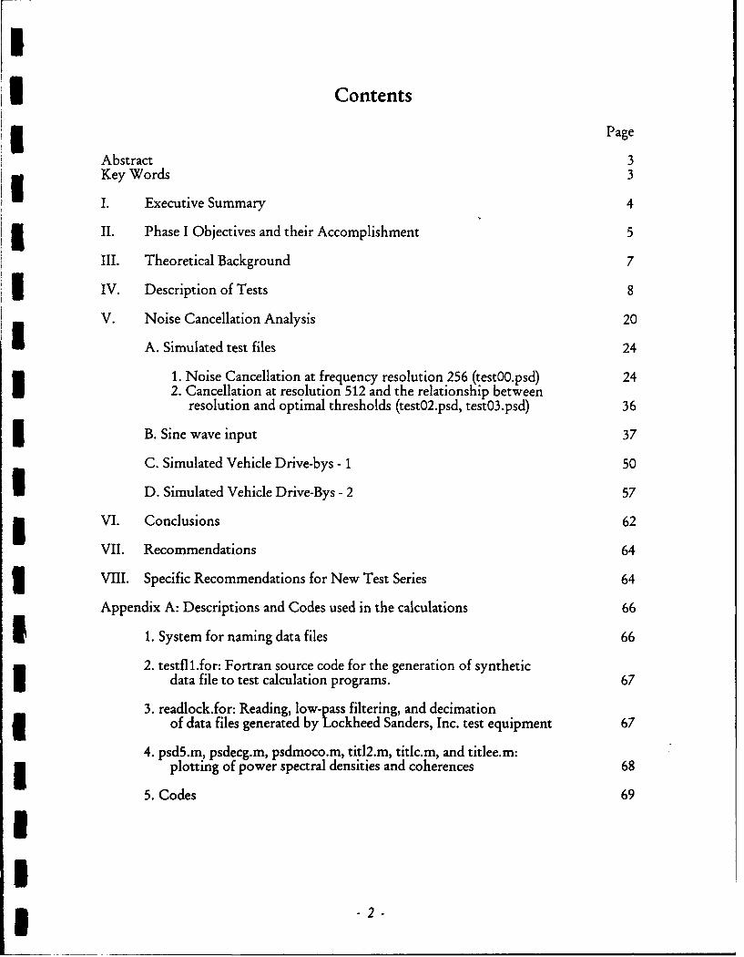
U Contents

Page

Abstract 3Key Words 3

I. Executive Summary 4

II. Phase I Objectives and their Accomplishment 5

III. Theoretical Background 7

IIV. Description of Tests 8

V. Noise Cancellation Analysis 20

A. Simulated test files 24

1. Noise Cancellation at frequency resolution 256 (test0O.psd) 242. Cancellation at resolution 512 and the relationship between

resolution and optimal thresholds (test02.psd, test03.psd) 36

3 B. Sine wave input 37

C. Simulated Vehicle Drive-bys - 1 50

I D. Simulated Vehicle Drive-Bys - 2 57

3 VI. Conclusions 62

VII. Recommendations 64

3 VIII. Specific Recommendations for New Test Series 64

Appendix A: Descriptions and Codes used in the calculations 66

1 1. System for naming data files 66

2. testfll.for: Fortran source code for the generation of syntheticdata file to test calculation programs. 67

3. readlock.for: Reading, low-pass filtering, and decimationof data files generated by Lockheed Sanders, Inc. test equipment 67

4. psd5.mn, psdecg.m, psdmoco.m, titl2.m, titlc.m, and titlee.m:3 plotting of power spectral densities and coherences 68

5. Codes 69

U2

IAbstract:

5 Some Army -vMWV armored personnel carrier vehicles carry air-acoustic sensor

systems comprised of a complement of roof-mounted microphones to detect and identify

other vehicles and aircraft such as helicopters. The performance of these systems tends to

become degraded as a result of the vehicle's own engine and road noise. Multi-channel

noise cancellation, if correctly applied, is capable of removing most of the own-vehicle's

engine self noise from the microphone outputs. The purpose of this project is to improvethe performance of these acoustic systems through the application of multi-channel noise

* cancellation.

The purpose of Phase I was to establish the efficacy of Signal Separation Technologies'

SFR-SFC (Signal-free Reference using Singular-value Decomposition) technique for

performing multi-channel noise cancellation for the aero-acoustic sensor application. This

efficacy has been firmly established as a result of Phase I tests and analysis. In a typical

example, a signal peak previously submerged in noise of the same level was made to stand

out over the noise by some 15 dB.

Also as a result of having conducted the tests and analyzed the measurements, we have

learned a great deal about vehicles and the effects of sensor placement.

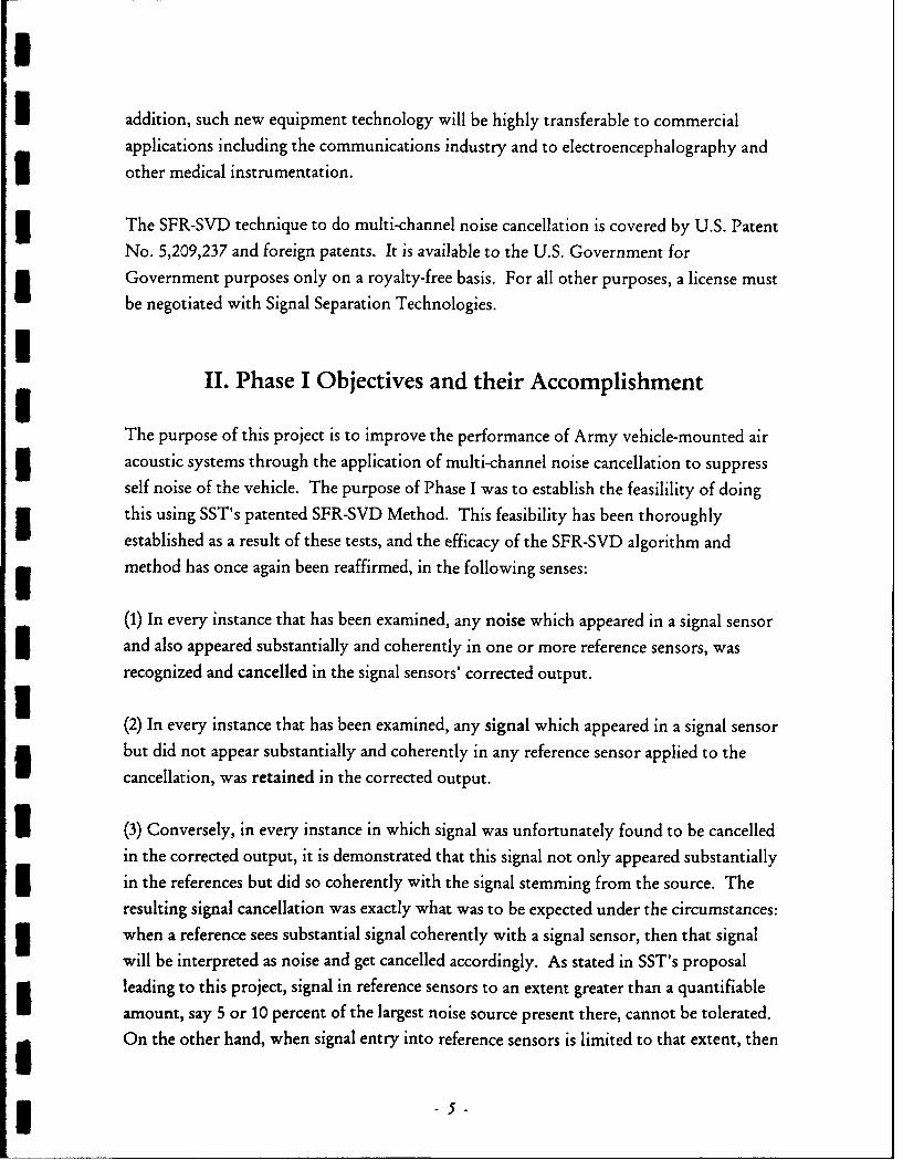
The SFR-SVD technique to do multi-channel noise cancellation is covered by U.S. Patent

No. 5,209,237 and foreign patents. It is available to the U.S. Government for

Government purposes only on a royalty-free basis. For all other purposes, a license must

be negotiated with Signal Separation Technologies.

Key Words:

HMMWV vehicle, Armored personnel carrier, Detection, Classification, Air-acoustic, .'Noise cancel(-ling, -lation), Self-noise, Signal Processing, Signal-free reference, Singular- 1

value decomposition, SFR-SVD Method .. on

By ________

Distribution I

Availability Codes

DsjAvail and/IarDist Special

3t

II

I. Executive Summary

Some Army HMMWV vehicles carry air-acoustic sensor systems comprised of a3 complement of roof-mounted microphones to detect and identify other vehicles andaircraft such as helicopters. The performance of these systems tends to become degradedas a result of the vehicle's own engine and road noise. The purpose of this project is to

improve the performance of these acoustic systems through the application of multi-channel noise cancellation.

The purpose of Phase I was to establish the efficacy of Signal Separation Technologies'3SFR-SVD (Signal-free Reference using Singular-value Decomposition) patented and widelytested technique for accomplishing this task. SFR-SVD is the only known method for3 correctly performing multi-channel noise cancellation. Its efficacy for the presentapplication has been firmly established as a result of Phase I tests and analysis. In a typicalexample, a signal peak previously submerged in noise of the same level was made to stand

out over the noise by some 15 dB. Signal-to noise improvements of 20 dB and more havebeen common in the past when the SFR-SVD method has been applied. The purpose of aPhase II project to be proposed is to perform additional tests needed to identify improvedsensor locations, particularly for the noise sensors, and then to develop a real time system5 to cancel the noise on line in real time.

3 Phase I began with an analysis of data previously taken by Lockheed Sanders, Inc. Sincethe available data did not contain signal, and since SST considered the measurement andanalysis of signal an essential part of demonstrating the worth of our methods, thisexisting data was used primarily to prepare the software and data formats. New tests wereconducted with Lockheed Sanders, Inc. at their facilities on June 2, 1994. The analysis of

these test results is reported in this document.

5 A Phase II project will be proposed to identify and test improved locations of sensors,especially reference sensors. Assuming this effort to be successful, the software will be5 adapted and built into a real-time multi-channel noise cancelling system. Such a systemwould find applications, not only in the aero-acoustic sensor interference problem, butalso in several other Army noise cancellation applications such as an endfire acoustic

detection array under development at Army Research Laboratories, and an acoustic sensorproject under development at the Night Vision Electronic Sensors Directorate. In

4-

I

I addition, such new equipment technology will be highly transferable to commercial

applications including the communications industry and to electroencephalography and3 other medical instrumentation.

3 The SFR-SVD technique to do multi-channel noise cancellation is covered by U.S. Patent

No. 5,209,237 and foreign patents. It is available to the U.S. Government for

Government purposes only on a royalty-free basis. For all other purposes, a license must

be negotiated with Signal Separation Technologies.

III. Phase I Objectives and their Accomplishment

The purpose of this project is to improve the performance of Army vehicle-mounted air3 acoustic systems through the application of multi-channel noise cancellation to suppress

self noise of the vehicle. The purpose of Phase I was to establish the feasilility of doing

this using SST's patented SFR-SVD Method. This feasibility has been thoroughly

established as a result of these tests, and the efficacy of the SFR-SVD algorithm andmethod has once again been reaffirmed, in the following senses:

(1) In every instance that has been examined, any noise which appeared in a signal sensor3 and also appeared substantially and coherently in one or more reference sensors, was

recognized and cancelled in the signal sensors' corrected output.I(2) In every instance that has been examined, any signal which appeared in a signal sensor

but did not appear substantially and coherently in any reference sensor applied to the

cancellation, was retained in the corrected output.

3 (3) Conversely, in every instance in which signal was unfortunately found to be cancelledin the corrected output, it is demonstrated that this signal not only appeared substantially

in the references but did so coherently with the signal stemming from the source. The

resulting signal cancellation was exactly what was to be expected under the circumstances:3 when a reference sees substantial signal coherently with a signal sensor, then that signalwill be interpreted as noise and get cancelled accordingly. As stated in SST's proposal

leading to this project, signal in reference sensors to an extent greater than a quantifiable

amount, say 5 or 10 percent of the largest noise source present there, cannot be tolerated.£ On the other hand, when signal entry into reference sensors is limited to that extent, then

I -5-

it is readily kept out of the required noise cancellation filters by an appropriate setting ofthe SFR-SVD eigenvalue cutoff thresholds, and the signal will then be preserved intact asit should.

In most cases during the June 2 test series, substantial loudspeaker signal energy was laterfound to have entered all the references, which in principle are supposed to get primarilyself-noise energy. Since this was the first such test series in which SST had participated,and since the primary purpose of the test was to verify the efficacy of our algorithms andsoftware for this application, we did not feel justified in suggesting substantial changes ofsensors or sensor locations from those which had been used in previous tests byLockheed-Sanders, Inc. Moreover, during the June 2 tests our most prevalent concernwas to get the loudspeakers close enough so that the microphones would hear them. Themicrophones on the far side of the vehicle from the loudspeakers did not hear themicrophones as well as those on the near side, and would probably be better mountedstanding up from the roof. But the main difficulty turned out to be too much signal inthe references.

Apart from sensor locations, another factor which may have affected the various sensor

coherences and hence caused signal cancellation was the fact that over most of thefrequency range of interest, the HMMWV and its sensors stood in the near field of theloudspeakers. In that region, the acoustic waves are nonplanar and may contain otherimportant nonlinearities. Since coherence has everything to do with whether a set ofsignals or noises are linearly related, this is not a trivial matter and must be more carefullycontrolled in subsequent tests.

In any case, the most important problem in the tests was the entry of too much signalinto the references, compared to the noise levels they received. Perhaps it would have

been better to run the HMMWV engine at a higher speed rather than idling, to increasethe noise levels. We are now convinced that optimal types and locations of all sensors,but especially the references, need to be determined through a carefully designedexperiment.

Thereore, the most important thing which remains to be done is to carry out such acarefully instrumented and controlled second experiment, in which source and noise

levels entering all sensors can be subjected to thorough spectral and coherence analysis on-site, and sensor types and locations can be adjusted in order to optimize the "noise to

6-

I

I signal ratio" in the references. It is demonstrated in Section VD of this report that

monitoring the various power spectral densities may not be sufficient in this regard; the3 coherences of the sensors with the source must be known as well in order to assure

intelligent choices for sensor locations. We are confident that efficacious reference sersors

types and locations will be found as the result of such a test. We hope that such a new

test would again be performed with the assistance of Lockheed Sanders, Inc., and wish to

take full advantage of the valuable experience these people have already accumulated on

this and related projects.

lIII. Theoretical Background

As stated in the proposal leading to this project, multi-channel noise cancellation in the3 context of separating signal from noise can only be accomplished correctly by using

singular-value decomposition on the noise correlation or cross-spectral density matrix.

This feature, which is the core of SST's multi-channel noise cancellation patent, is

essential in order to eliminate all redundancies in the noise matrix, and in order to prevent

signal cancellation when even the minutest amount of signals enter a noise sensor. But

even when SFR-SVD is applied, signal must not enter the reference sensors at levels as

large as those of the noise found there. When that happens, a threshold which is able to5 ignore the signal in the noise sensors, while utilizing the noise found there for filter

calculations, is not attainable.

As has been stated in the proposal on which this project is based, effective multi-channel

noise cancellation requires that the noise measurements used for cancellation must have

two essential characteristics: (1) They must contain the noise to be cancelled coherently

with the noise appearing in the signal sensors, and (2) they must contain no more than a3 modest amount of signal, relative to the noise that they receive. (There is some leeway in

tolerable levels, but a signal level equal to the largest noise level would be excesssive,

* because then there would be no threshold which will keep noise but reject signal from the

filter calculations). Analysis of coherences and power spectral densities calculated from3 the June 2 tests show that the first requirement was generally met, while the second one

was not met to a sufficient degree. The result was that for the cases of greatest interest in3 the June 2 tests, the signal was cancelled along with the noise.

I1 .7-

IThe code used for the analysis was a single-pass code, which calculates a single set of cross-

Sspectral density matrices (CSD's), averaged over the entire time interval of interest. Thesematrices are used for the calculation of the Wiener filters that condition the noise before it3 is subtracted from the signal. The code is a modification of a single-pass code which hasbeen used in the past for the analysis of batch mode fetal electrocardiograms. Analternative code would be an adaptive one, which continually updates the CSD's and also

permits the continuous plotting of the corrected time series. The single-pass code waschosen for this analysis because of its greater simplicity and because it conveniently

I presents spectral information of signal and noise over a selected time span.

I A word is in order on the meaning of "coherence." Coherence as plotted in the figures isthe absolute cross spectral density between two sensors, normalized by the square root ofthe product of the two individual power (auto) spectral densities. Often in the literature,the coherence is taken as the square of this quantity. The reason we prefer to work withthe square root of the usual function is that that square root is the complex Hermitian

analogue of the readily visualized absolute-value cosine-of-the-included-angle between twovectors in an ordinary real n-dimensional vector space. It thus represents the degree of3 linear dependency vs. orthogonality between a pair of signals (or noises). Either way, as

an absolute-value cosine or a cosine-squared, of course, the coherence is always between 0and 1.

1 IV. Description of Tests

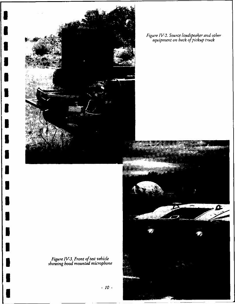
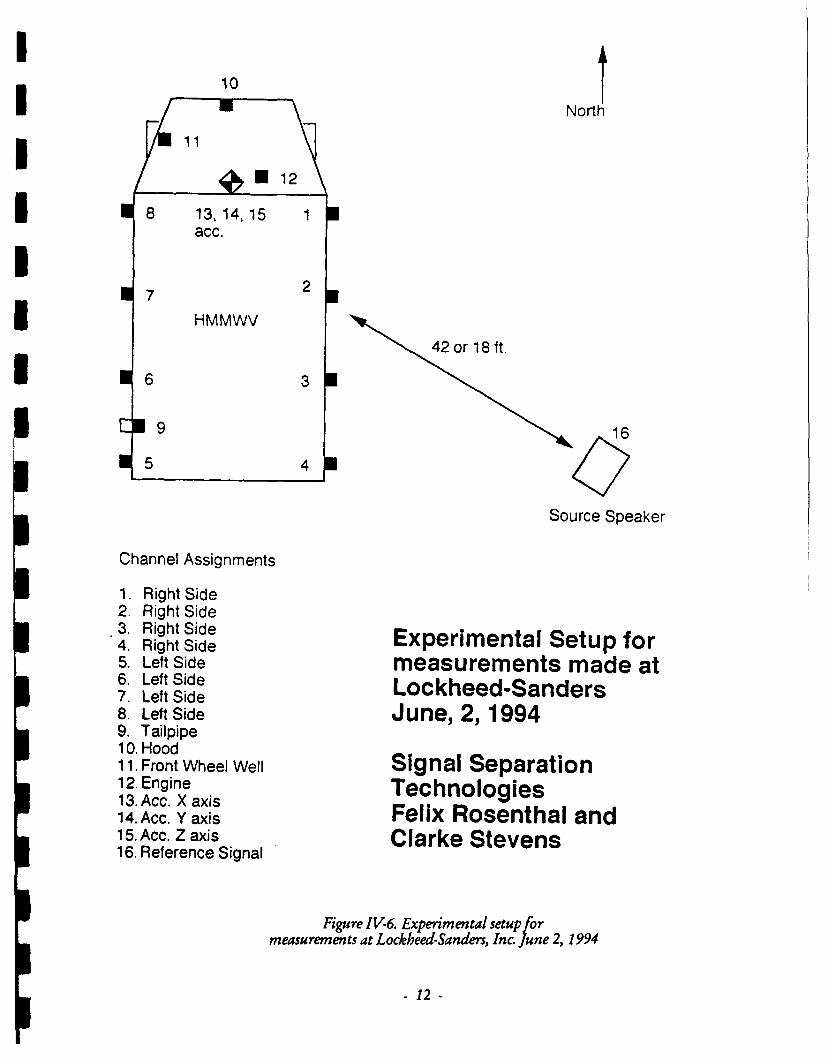
I A day-long series of tests was conducted at Lockheed Sanders, Inc. facilities on June 2,1994. Figure IV-1 is a photograph of the test vehi-le standixng in front of Lockheed3 Sanders, Inc.'s instrumentation shack. Figure IV-2 shows the loudspeaker and otherinstruments mounted on the back of a pickup truck, while Figure IV-3 depicts the front3 of the test vehicle showing the hood-mounted reference microphone. Figures IV-4 andIV-5 show the mounting of the tailpipe and front wheel well reference microphonesrespectively. The experimental setup is illustrated in Figure IV-6, showing the relative

location of the HMMWV vehicle, its sensors, and the source loudspeaker system. Most of

the instrumentation was located in a nearby instrument shed. The channel assignments

listed in Figure IV-6 indicate the channels assigned to each of the 16 sensors: the 8 primary

3 -8-

IJ

IMIN

44Iw.. ... .

FiueI-1UM W etvhcesoi ofmcohnsstnigIfoto~che adrs c ntuetto hc

IFigure IV-2. Source Zoudspeaker and other

equipment on back oj pickup truck

II

II

�

I iK:'IIIIU V

II

Figure 117-3. Front of test vehicleI showing hood mounted microphone

I1 .10-

II Figure IV-4. Tailpipe microphone

UIIIIIIIIII3IUI

Figure IVS. Wheel well microphone

''f

__ ____ _____________________________

10

North

11

0 8 13,14,15 1acc.

7 2 0

HMMWV

S6 3 0

5 4 1

Source Speaker

Channel Assignments

1. Right Side2. Right Side.3. Right Side Experimental Setup for4. Right Side5. Left Side measurements made at6. Left Side Lockheed-Sanders7. Left Side8. Left Side June, 2, 19949. Tailpipe10. Hood11. Front Wheel Well Signal Separation12. Engine Technologies13. Acc. X axis14. Acc. Y axis Felix Rosenthal and15. Acc. Z axis Clarke Stevens16. Reference Signal

Figure IV-6. Experimental setup formeasurements at Lockheed-Sanders, Inc. June 2, 1994

- 12 -

ICurb Side

Front

1A3 A2 Al AO 225"

I o , -1 0o

3 \3.5" \15 / '8"

*.•" K"10 Roadside

I 0

I 511

I ~2'9.25" 3'2" 3'1 1.5"

I 0

Exterior mounting locations of the sensors on the HMMV

2 June 1994U

Figure IV-7. Exterior mounting locations on the HMMWV,June 2, 1994

- 13-

CO.

N IU L. r- "P V E

N~ N 0- x

O in 0 a B 8

EE

t ~~36 Ch U -C VE r

0M

E IL

u~ N a::< 0

CZI -3 iO i 0

3~~~ Acelrmee tye32

I.1 -141

II

II I I I

C •1 I I i'

•'- -- o o o

gI. 0r,0)

to ow

0 00) W 0' 0* ~

I] i ,CJ - 0 0

cs0 004 0 0 0 00E

0 00 0 0-00o

C 'j'j2j' ca ~ (aj (a w)2 4 4

1~15-

!0CL~~~~1 -0- 00 1I2t .

Lockheed Tape Log

Run 1 (Tape5) 51Engine off, reference directly connected

Event Offset i Real Time CommentStart tape 0:00:00: 9:14:23;1 kHz sine wave starts 0:01:00 9:15:231;1 kHz sine wave stops I 0:02:00 9:16:23.500 Hz sine wave starts 0:03:001 9:17:23500 Hz sine wave stops 0:04:00! 9:18:23_250 Hz sine wave starts 0:05:00_ 9:19:23_

250 Hz sine wave stops 0:06:00 9:20:23125 Hz sine wave starts I 0:07:00 9:21:231Gun shot 0:07:17 9:21:40_

jet low amplitude 0:07:371 9:22:00!25 Hz sine wave stops 0:08:00! 9:22:23 i100 Hz-1 kHz sine wave sweep starts 0:08:56: 9:23:191100 Hz-1 kHz sine wave sweepstops I 0:09:561 9:24:19

sound file e04a2063 starts 0:10:56i 9:25:19horns t 0:12:37i 9:27:00;sound file e04a2063 stops I 0:12:52, 9:27:15sound file e04a2066 starts 1 0:14:52'; 9:29:151sound file e04a2066 stops - 0:16:06' 9:30:29

I sound file e04a2070 starts 0:18:06' 9:32:29:et fly-over - 0:19:37 9:34:00:

sound file e04a207O stops 0:20:07 9:34:30_ _i pro~op p!ane fly-over 0:20:37 9:35:00

sound file e04a2071 starts .. 0:21:57: 9:36:20 ...sound file e04a2071 stops___ 0:23:05: 9:37:28 ...i Stotape 0:23:09, 9:37:32

Run 2 (Tape 4) , _encgine off, microphone on sourcesea ker_____

Event 1 Offset 1 Real Time: Comment_St-art tape i 0:0000 10:01:00. 0'gun shots 1 0:01 :00 10:02:00O1 kHz sine wave starts j 0:01:001 10:02:001

I 1 kHz sine wave stops 0:02:00 10:03:001500 Hz sine wave starts 0:0 3:00- 10:0 4 :00-500 Hz sine wave stops 0:04:001 10:05:0)01

I 250 Hz sine wave starts 0:05:00! 10:06:00250 Hz sine wave stops 0:06:00: 10:07:00125 Hz sine wave starts 0:07:00, 10:08:001U 25 Hz sine wave stops 0:08:00 10:09:00 ,100 Hz-1 kHz sine wave sweep starts 0:08:56! 10:09:56__100 Hz-1 kHz sine wave sweep stops 0:09 -:56• 10:10:56-I sound file e04a2063 starts 0:10:56, 10:11:56:sound file e04a2063 stops 0:12:52 10:13:52

3 Table 1. Lockheed tape log, p. 1

16 -I

Lockheed Tape Log

Isound file e04a2066 starts 0:14:52. 10:15:5 2______sound file e04a2066 sops 0: 16:06: 10:17:06__sound file e04a2070 starts 0: 18:06' 10:19:06sound file e04a2070 stops 0:20-07; 10:21:07'_____sound file e04a2Q71 starts 0:21:57 - 10:22:57 ___

sound file e04a2071 stops 0:23:05, 10:24:05 ___

Stop tape 0:23:09 10:24:09

I ~Run 3 (Tape 31 1___engine running, microphone on source speaker1 ___

Event Offset___ Real Time CommentStarttpe 0:00:001 10:26:QOhelicopter flyj-over 0:01:00:, 10:27:00 ____

1 kHz sine wave starts T 0:01:00 10:27:001EI kHz sine wave stops 0:02:00W 10:28:00 _

prop pla.n-e.0:02:00 10:28:00 -

500 Hz sine wave starts 0:03:00 10:29:00 _I 500 Hz sine wave stp ___-__ 0:04:00 10:30:00 _ ---

250 Hz sine wave starts 0:05:00 10: 31:00250 Hzsine wave stops___ 0:06:00 10:32:0025 Hz sine wave starts 0:07:00 10:33:00 _

2 5Hz sin waest 0:.08:00'-. 10:34ý:00 -_____

100 HzFf-i kH~z sin~e wave swyeep sta~rts 0:08: 56' 1:45I 100 Hz- I kHz sine wave sweep stqps 0:09:56 _ 10:35:56 _

sound file e04a2063 starts 0:10:56 10:36:56sound file e04a263tos__ iiq:252~1:8:2--E sound file e04a2066 starts 0:14:52 10:40:52 _

sound file e0aO6stops 0:16:06 10:42:06__sound file e04a2070 starts 0:18:06 10:44:06 __

sound file e04a2070_stops 0: 20:07 10:46:07vhcedrive-by _ ___0:21:30 10:47:30 -

sound file e04a2071 starts __ 0::5. 10: 47:5S~ound fileje04a2Q71 stops . 0:23':05! 10:49:05Stp tap ______:23:09,l10:49:09

*u__ (Tap_ _ __ _

engine off, source speakers moved to 18 ft. frmvehicle, 2 amplifiers, HF and- LFf(20-100 Hz)--.Event _______ Offset iReal Time Comment

,-i-ki--s__n__ewa__e__start 0:01:00: 1_1: 39:2 3I ikHz sine wave stops 1 0:02:00 11:40:23 __

500OHz sine wave starts I 0:03:00: 1l4 : 3500 Hz sine wave stops I 0:04:00: 11: 42:23'I Truck drive-by _____ __i 0:04:37; 11:43:00'250 Hz sine wave starts -- 1 0:05:00 11:43:23

3 Table 2. Lockheed tape log p. 2

I -17-

3 Lockheed Tape Log

I250 Hz sine wave stops 0:06:00 11:44:2325 Hz sine wave starts I 0:07:00; 11:45:23.;25 Hzsine wave stops 0:08:00 11:46:23'I100 Hz-i kHz sine wave sweep starts 1 0:08:56 11:47:19100 Hz-i1 kHz sine wave sweep stops 0:09:56ý: 11: 48:19 _________

sound file e04a2063 starts 0: 10: 56! 11:49:19'__________I jet fly-over 0:1:3~71 11: 51:00 _________

sound file e04a2063 stops I 0:12:52: 11: 51:15 _________

sound file e04a2066 starts I 0: 14:5 2 11:53:15'1_____sound file e04a2066 stops 0: 16:06: 11:54:2 9'I sound file e04a2070 starts 0: 18:0 6: 11:56:29__sound file e04a2070sjýpps 0:20:07 1 11:58: 30sound file _0a-d- starts__ ____ 0:2:5 1:C:20_____sound file e04a2071-stops 0:23:05>12:01:28;

* Stp tape ___I 0: 23:09--- 1-2-:01-:3-2 __ _

Run__5 _(Tape I) _ _ _ _ _ _ _ _ _ __ _ _ _ _ _ _ _

englrff!E running source..speakers moved to 18 ft. from veil,2a iirH n LF (0100 HzI - --.-. _ _ -Een Offset_ Real _Time _Comment

Start tape ___0:00:00, 12:16:40 phantom jpower supply used1 kHz sine wave starts _ _0:01:00 12:17:40'_prop pi[an 0:120 - 12: 18-: 0 0_ _-.

1 kHz sine wave stops 0__ 0:2 :600 -1:8:-4 0-__U 500 Hz sine wave starts _ __ 0:.03:.00 12:19:40.500 Hz sine wave stops 0:04:00 12:20:40'..prop plane __-0:04:20, 12:21:00__250 Hz sine wave starts L 0:05:00 12:21:40 __I 250 Hz sin-e-wave stops -0:06:00 12:22:40:25 Hz sine wave' starts . . . .0:07:00! 12:23:40 -

25 Hz sine wave stops 0:8:00 12:24:40 _

prop plane- ___ :820, 12:2 5:0.0 __

100 Hz- I kHz sine wave sweep starts ' 0:08:56 12:25:36 __I 100 Hz-i1 kHz sine wave swe.pq2s--p 0:09:5-6- 12:-26:36-so0Und f ilee e0-4 a 2-063j s-t-arts 0:10:56 12:27:36 ______

sound file e04a2063 stops 0:12:52, 12:29:32 ________

sound file e0a2ý66-starts 0: 14:5 2ý 12:31:32I sound file e04a2066 stops 0: 1S: 0 6 12:32:46 "Some source clipping-sound f ile e04a207O starts 0: 18 061; 12:34:461 iSome source clippjp~gsound file e04a207O stops I 0:20:07 i 12:36:47;Some source clipping-I sound file e04a2071 starts ___I 0:2 1:57; 1 2:38-:37 L__

soun fie e4a20 1 top 0:23:0 12:39:45--Stop tape_ 0:23:09 12:39:49 __

* Run_ 6_ (???)-- ___ _ ----

* engine off, source speakers moved to 18 ft. from vehicle, 2 amplifiers, HF and LF (20-100 Hz) -

3 ~Table 3. Lockheed tape log& p. 3

* -18.

Lockheed Tape Log

Event I Offset i Real Time CommentStart tape 0:00:00i 12:42:00 phantom power supplyused1 kHz sine wave starts 0:01:00p 12:43:00

1 kHz sine wave stops 0:02:00 12:44:00500 Hz sine wave starts 0:03:00 12:45:00prop plane 0:03:001 12:45:00500 Hz sine wave stops 0:04:00' 12:46:00.250 Hz sine wave starts 0:05:00 12:47:00250 Hz sine wave stops 0:06:00 1 2:48:006r - "I 25 Hz sine wave starts 0:07:00 12:49:00.25 Hz sine wave stops - 0:08:00j 12:50:00-100 Hz-i kHz sine wave sweep starts 0:08:56: 12:50:56 ...... .. -..

100 Hz-I kHz sine wave sweep stops i 0:09:561 12:51:56.sound file e04a2063 starts 1 0:10:561 12:52:56,sound file eO4a2063 stops 0:12:52 12:54:52sound file e04a2066 starts 0:14:52 12:56:52sound file e04a2066 stops . 0:16:06 12:58:06sound file e04a2070 starts 0:1 8:06 13:00:06prop plane 0:19:00 13:01:00sound file_e_04a2070St0stqp_ - 0:20:07. 13:02:07 .soundfile_e04a2_7._starts 0:21:571 13:03:57sound_file e04a207I stops 0:23:05 13:05:05 .

I Stop tape 0:23:09 1 3:05:09

II

UII

II

Table 4. Lockheed tape log, p. 4

5 -19-

II

I sensors were recorded on the *.gl file (ch. 1-8), while the seven references (9-15) and the

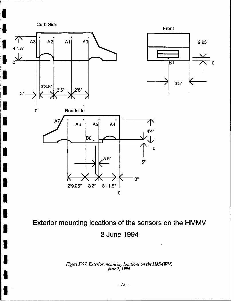
source (16) were simultaneously recorded on the *.g2 file.UFigure IV-7 shows the mounting locations of the sensors used on the HMMWV on June

2, while Figure IV-8 describes the accelerometers used in the experiment. Figure IV-9

provides calibration data for all sensors. Group A sensors 0 to 7 correspond to the

* primary sensors 1-8 as used throughout this report; Group B sensors 0-6 denote the 7

reference channels 9-15, while sensor 7 provided the source signal, channel 16.

U We made 5 test runs. The corresponding tapes were numbered in inverse order, starting

with Tape 5. (s. Lockheed tape log, Tables 1 - 4). For tapes 5, 4, and 2 the HMMWV3 engine was turned off; only tapes 3 and 1 contain own-engine noise. Of the two tests

containing own-engine noise, Tape 3 was improperly recorded; Tape 5 was therefore used

* for most of the analysis herein. Unfortunately, this tape was recorded with the

loudspeakers at a shorter distance from the vehicle than was the improperly recorded3 tape; it is possible that Tape 3 would have contained somewhat smaller near-field effects.

For each tape, several sine wave notes, and recordings of several vehicle passbys were

U played on the loudspeakers according to the log schedule. There were a few "sounds of

opportunity" such as gunshots and an airplane flying overhead.

* V. Noise Cancellation Analysis

We processed both simulated and real data. The simulations verified software operation,

and the analysis of the real data (pure tones or simulated drivebys broadcast over a

loudspeaker system) showed that noise cancellation as well as signal preservation took

I place in exemplary fashion whenever the data supported it. Analysis of the data also

served to prove that much of the time, far too much signal reached the reference sensors,

Sresulting in substantial signal cancellation.

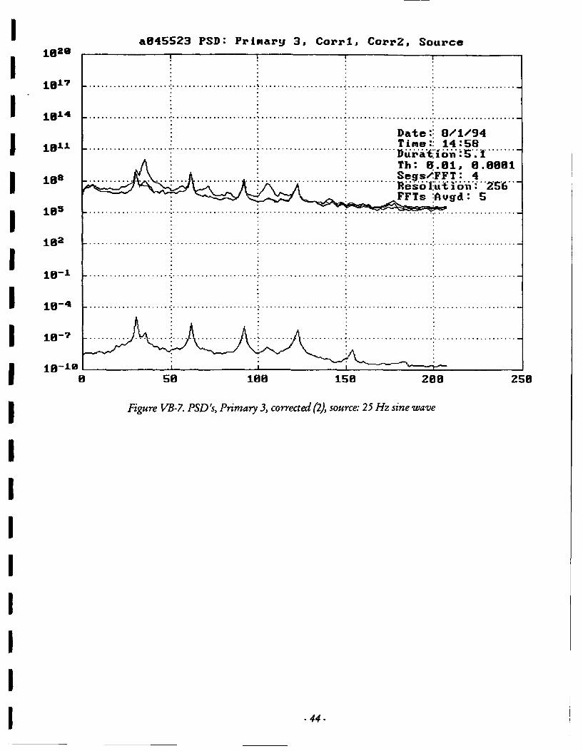
3 A good example of noise cancellation is given in Figure V-i, representing a 5.1 second run

taken from Tape 1 or a where the loudspeakers were playing a 31 Hz tone. This tone is

found 7 minutes and 35 seconds, or 0455 seconds, into Tape 1 or a, as identified by the

label starting with the file number a0455 in the Figure's title. (Conventions used in

labelling file names are described in Appendix A.)

* -20 -

U a045521 PSD: Primary 1, Corrn, Corr2, Source

I1 @1 1 4 . ...................... . . ........... .... ........ ... .... ..... ............. .... ... .. .... ....... ..... .

Date:: 8/1/94

S.................... ....................... . . .............................. b t i a £ .. "....": .. .. .. ........ .

Th: 0.01, 8.8081I .......................... ..-. ......... ............ S eg s/F F T- 4

i FTs gd: 5

S10 -5 . .... ....... . .. ... ..: .... .. ............... :. .......... ........ ,............ .... ..... i..... .. .... .... ....... .

S 1 0 _ 4 . ......... . ............................... .. ................... .:.... ...................... ..... .... .......

I L - ..............................I ................... ...........JlO-10 mJ

5a SIB ISOIS 200 258Figure V-1. Noise cancellation resultsfor 25 Hz tone using

S~4 of 7 references: Uncorrected, Corrected a, Corrected b, and Source.

I

I1 5-

I .1

I a845521 PSD: Primary 1, Corrn, Corr2, Source

S1 0 1 4 . ... . . ... . . ... . . . .. .. ....... .............. . ......... . . . . . ..... . ..... ...... ... ... .. .. : .. .. . .. .............101

Date: 8/1/941U1 Tiwe: 14:58

: Duration :5.1ITh: 0.81, 8.0081l o g ...... ..... .. ..... ..... ... .... ...... .: ............. ........ ........ ........Resolution: 256SFTs gel 5

1 .... .. .... ... . .. .. .. . .... ............. .......... .... . .. . . ... .... : ...... ........ . ... ...• .. .... . .............

I 18-1

I 1_I 1 8 _ 4 ................................................................. : ..................... ................ ..

l 1.-. ................. .

to-Is I 58 188 158 280 258

Figure V-2. Same as Figure V I but with Uncorrected and thetwo Corrected curves overlaid/or easy visual comparison

IIIIIII* -22-

II

The uppermost curve represents the raw (except for low pass filtering) output of themicrophone designated as primary sensor 1. The bottom curve shows the sourceloudspeaker signal as picked up by a microphone placed on top of the speaker. Curves 2and 3 respectively are two versions of the noise-cancelled output of Primary sensor 1,using eigenvalue cutoff thresholds respectively of .01 (20 dB) and 0.0001 (40 dB) as shownas "Th:" in the identification block of the figure.

Three large harmonics show up respectively at 62, 92, and 123 Hz. The peak at 31 Hz is

accompanied by another, smaller, peak at about 35 Hz.

Turning to the uncorrected primary at the top, we see broad bands of engine noise around65-80 Hz as well as 100-115 Hz. In the corrected curves, this engine noise has beenremoved while the source peaks remain at substantially their uncorrected level. (Thesmall source peak above 150 Hz appears to never have made it to primary sensor 1.) It isi. oted that in the corrected output, especially in the second or 40 dB version, the twin

peaks at 31-35 Hz have substantially the same shape as in the source, whereas the relativemagnitudes of each twin are highly distorted by engine noise in the uncorrected version.

To permit better visual interpretation of the actual noise cancellation and signal retention,the top three curves, uncorrected and two version of corrected, are shown overlaid inFigure V-2. This overlay makes it very clear that the signal has been completely3 preserved, while a substantial quantity of engine self noise extending over the entirefrequency range has been eliminated. In terms of signal to noise improvement, the signalstands out some 15 dB over the noise in the corrected versions, whereas it was submerged

in the uncorrected one, suggesting a signal to noise improvement of some 15 dB. Thisimprovement is not atypical for the SFR-SVD Method - improvements of up to 20 dBand more have been common in past experience. Figure V-2 also demonstrates that thenoise cancellation is able to separate signal from noise even when their frequenciescoincide, as is the case in the 30-40 Hz range of frequencies. This range clearly containsnot only the twin peaks at and near the source fundamental frequency, but it alsocontains the fundamental range of frequencies of the vehicle engine, and the noisecancellation program clearly has no difficulty in separating the two. Noise some 20 dB inexcess of the signal was successfully eliminated while the signal remained completely

intact.

3323 -

I

I In the run shown in Figures V-1 and 2, only four of the seven references were actually

applied. This run and its ramifications are discussed at greater length in Section VB.

A. Simulated Test Files (files test0"-.psd)I1. Noise Cancellation at frequency resolution 256 (test0O.psd)

I To verify the correct application of the noise cancellation software to the problem of

passive aero-acoustic sensor self interference cancellation, the software was tested using a

synthetic sine wave record generated by program testfll.for. In Figure VA-1, the channels

are shown consecutively as 8 "primaries" (curves 1-8), 7 "references" (9-15), and the"I"source" (16). Each vertical division represents a factor or 10'6 or 60 dB.

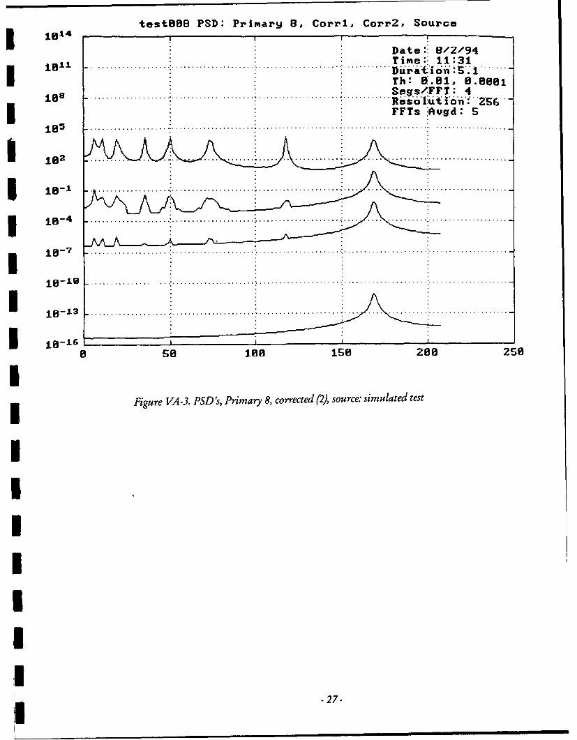
Each reference channel (ch. 9 - 15) consisted of a single sine wave at a frequency unique to

that sensor. The seven simulated noise frequencies were 7, 11, 20, 36, 50, 74, and 119 Hz

respectively. The reason they do not appear as "line" spectra is of course the result of the

effectively rectangular window used in the FFT calculations. The source channel (16)

likewise was a single sine wave, in this case 170 Hz. The primary channels were chosen as

linear combinations of the reference and source signals. None of the primaries except

Channels 7 and 8 contained the source frequency, with the result that no significant signal

peaks show up in their corrected power spectral densities. Primary Channel 7 (Fig. VA-

2), on the other hand , contained equal amplitudes of the two references at 74 Hz and 119

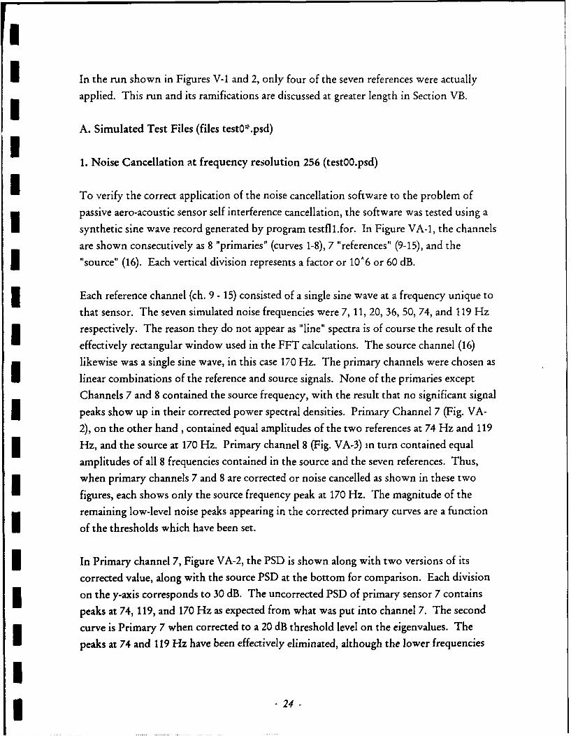
Hz, and the source at 170 Hz. Primary channel 8 (Fig. VA-3) in turn contained equal

amplitudes of all 8 frequencies contained in the source and the seven references. Thus,

when primary channels 7 and 8 are corrected or noise cancelled as shown in these two

figures, each shows only the source frequency peak at 170 Hz. The magnitude of the

remaining low-level noise peaks appearing in the corrected primary curves are a function

of the thresholds which have been set.

In Primary channel 7, Figure VA-2, the PSD is shown along with two versions of its

corrected value, along with the source PSD at the bottom for comparison. Each division

on the y-axis corresponds to 30 dB. The uncorrected PSD of primary sensor 7 contains

peaks at 74, 119, and 170 Hz as expected from what was put into channel 7. The second

curve is Primary 7 when corrected to a 20 dB threshold level on the eigenvalues. The

peaks at 74 and 119 Hz have been effectively eliminated, although the lower frequencies

II -*24 .

U 'test88 Channels 1- 16

* 0 Datei :0/134Time'.: 14:20

* . Durat-ion:5.1-J ...."...... .......... ....... ....................... Rese.hl i o ,;.n 2Z 56..-!

I 1-

I

I

l1 8 -2 5 .. ......... .................... ....... ...... . . . . . .

o 1 - 437 .................. .. . .. .. . . -...-"....--.......

I1- ---- "-05s 188 158 288 258

Figure VA-i. PSD of all 16 channels. simulated test

I3 -25-

test@07 PSD: Prinarg 7, Corni, Carr2, Source

3f .Dte:: /29

te l ............... ........................... ............... D ............

Th: 0.01, i8.0081

188 ................ ..................... .................... ...........I FFTs Augd: 5

I0 ........................ ................. .........1I ...................................... .........

a so lee Ise 200 250

Figure VA -2. PSD 's, Primary 7, corrected (2), source: simulated test

-26

testO08 PSD: Prinargj 8, Corrn, Corr2, Source3LJL* Date: 8/2/94

Time:: 11:31

* ~Th: 0-0j, 080Segs/FFT:4

* ~FFTs :Avgd: SIL 5 .......... .. ....... ......... ...I. .......... ..... .........

j0 .... ...... ..... ...

...I. ................

1 0j -4 ' ............ ..5 8. ... .... .. ........ ..10.. 1... 2 88.2.8

IL - ......................... .......................3. .. .. Fig. ..... ...re. ... ..... ... ... ..... P. ... ... ... ..'s Pri.....co rec ed (2 ,.sur e:.im lat d.es

I0 1 ........................ ......... ....... ................ .....

I L-1

3~- 27-

testO8 Coherence: References 9, 1@, 11, 12, 13, 14, 15

Date:! 8/2/94Time:: 11:31

Duration: 5.1.. ...... ........... .. . . . . ....... ... ................. . ..... ...e ~ ~ .JSegs/FFT: 4Resol:ution: 256

FFTs :Avgd: 5- 1 .. . . . . .• - - • --- .. . ; - : ... . . .. . . . . . . . . . . . . . . . . . . . . . . . ..

- 2i . .. ..... ... .. ... .. .. '..................... ... ................. ................ ..... .. ..................

I -25............................. ... .................

1-4

8 5s 1i0 15 286 258

Figure VA-4. Coherences of references with source: simulated test.(Note: Since the simulated test constituted deterministic sine waves,

not stochastic functions, these coherences have no physical significance.)

S- 28.

testOB PSD: References 9, 10, 11, 12,, 13, 14, 15, Thru: 16103 ..... It..

. . . . . . ... . . . .. ........................ ....

I Resolution: 256

.................. ........I ..................... ... ......

.... ...........................*. ........... ...:. .....

.I. .... .. .........I... .

I. .... ............... ........18 2? . ... ........

............ ...10..10.200.2. ........I .......Figure ...... ...... Is References .... ..nd source. sim.lated.test

.I. ............... ............... ..........

.. ...3.. .... ... ..9. ..

3 testOl Coherence: References 9, 18, it, 12, 13, 14, 15

Date:: 8/4/94Time:: 11:49

Segs-oFFT : 4Resolution: 512FFTs:Augd: 5

3 -2. .. ... .....

-68 503 108 1S0 200 258

Figure VA-6. Coherences as in Fig. VA-I, but withI 512 resolution: simulated test; no physical significance

I30

testOl FSD: References 9, 18, 11, 12, 131 14, 15. Thru: 16

1@2 .. ... .... ..I ... . .. .. ... I ... ..4. .. . At o-: 13/4 /94

3 1 . .................... .. .. .. .. ..... ton

........B. ....: ' ...

80 -... ..... ... 1..0..2....25

.......... .... ~ ~ F g r .. .... .. .... ... ... .. .. .. .. . .s.Ref ren es.nd.our e.a..

Fig ........ ........but..with..512...resolution.....sim ul..ted..test.......... ......................... ......... ........... ............I. ... ............................ .......

.. ...... ..............IL -8....

.......... ... .. ....

....... .............. ............ .. .- 31.. .. ..

test017 PSD: Primarj 7, Corrt, Corr2, Source@ Date:! 9/4/94

Time:: 11:491esFTDuration :5.1

S.. ... .. ... .. ....................... .. ..... ....................... R e s o lti o n S"B .1"2"B 8 8............. Resol:ution: 512

1 OB L ..................... ............... ... .............. .......... . . ............ F ~ 'i • d 5.........

1S .............................. ................... .. ......

.... ... ..... . . . . . . . . . . . . . . . . . . ... . . . . . ... . . . . . . . . . . . . ....... . . . . . . . . . . ... . .. . . . .. . . . .. . . . . . . _

S_ 5 . .. .. .... . . ... . . ... . . . ... ........... ...... .......... . . ... ... ... .. . . . . . . ... .. .... . . .. .............

1BO-17 !

0 50 100 150 208 250IFigure VA-8. PSD's, Primary 7, corrected (2), sourceSas in Fig. VA-4, but with 512 resolution: simulated test

IIIIU1 .32-

1013 testOlO PSD: Primary 8, Cornl, CorrZ, Source

DateV /49Time:: 11:419

181 . .. ... .. .. ... ...... ... .. .. ... .... ... .. .. .. Durat ion :5 .1

I Segs/ýFFT: 4107 ................ ................ Resolution: 512

1 0 4 ~~~~~~~ ~ ~ ~ r s u d ... .. .. ........I ...... .......... ..............

IL J ......... ....... ... ..... .........IL - ..... .............. ............... .........

18 5 ............ .. ..... ...:. .......... .. ...... ....... ..

SO5 100 ISO 280 250

Figure VA-9. PSD 's, Primary 8, corrected (2), source

as in Fig. VA-5, but with 512 resolution: simulated test

I33

Stest827 PSD: Primarg 7, Corrl, Corr2, Source

5Date:. 8/4/94Time:: 12:23

isle ..... Duration :5.1I @ 1 . . .. .. .. .. .. . .. : ... .. ... .. ... . ' .................... . ............ aTh .1 . i ffn 8 .... 1 e - 81619 ':B.saei1, :ie- B 6

Segs./FFT: 4.................... ...................... R e so l:u t io n : S 12F F T s i> da - "s . . . . . . .

" " -5 .............. .............-... .. .. ..... .. .. ... .. .. ....-e . . . . . . . . . . . . . . . . . . .. :. . . . . . . . . . . . . . . . . . . . . *. . . . . . . . . . . . . . . . . . . . . - . . . . . . . . . . . . . . . . . . . . •. . . . . . . . . . . . . . . . . . . . .

10-87

0 5s 108 15 280 2S8

Figure VA-iC. PSD 's, Primary 7, corrected (2), sourceas in Fig. VA-8, but with 512 resolution: simulated test

-34-

ItestBZ8 FSD: Primargp 8, Corrn, Corrn 45 i e.............. .... .............: .. . .. . .. .... .. .. .. .. .. .. .. .. .. .. .. .. .. .. .............. i o s. • :.. .....i " ~~................................. . . . . . . . .. . . . . . . .......... F .F. s 21 g • ; 5 i -............ .

..... .. .. . ....... . ......... ..... ..... .. • ......... ........... • ............. t . . . . . .. 27.. .. . .

.......... ~ ~ *........... :..................... "....................." ............ . . . . . . . . . .............. .. ... .. . .. . .. .... : ..... .... ............ ; ......... . . . ... . . .. . . .. ... ......... . .... .. •..... .. .. .. . .. ... ...

i.. . . . . .

iS~*... .. *.*.. ....... ...................... . . . . . . . .................................... . . . . . . . . .

S... .. . .. . .. .. . . . ... .;...... .... ............ ; ......... . . . .. . . ... . •. .. ... . ........ . .... . •... . . . . . . . . .

S. . . . . . . . . . . . . . . . . . . .•. . . . . . . . . . . . . . . . . . .. . -. . . . . . . . . . . . . . . . . . . . -. . . . . . . . . . . . .. . . . . . . . •.. . . . . . . . . . . . . . . . . . . .

5 1_•

858 188 158 288 258

IS~Figure VRA-i1. PSD 's, Primary 8,.corrected (2), sourceas in .Fig. VA-9, but with 512 resolution: simulat.ed test.

II£

IIU1 -35-

I

-- do appear some 30 dB below the source peak at 170 Hz. When the eigenvalue threshold is5 set to 40 dB, the resulting corrected curve appears remarkably like the source signal.

Figure VA-3 shows the PSD of primary sensor 8, its two corrected values, and against the

source. In this case as expected, the uncorrected primary shows all eight frequency peaksas put there. The 20 dB threshold corrected PSD lifts the source channel at 170 hz some20 dB above the highest "noise" frequency at 7 Hz, while the 40 dB correction providessome 40 dB of protection against the highest noise level at 119 Hz. Again, the lower

threshold value eliminates more of the remnants of "noise" frequencies in the primary.

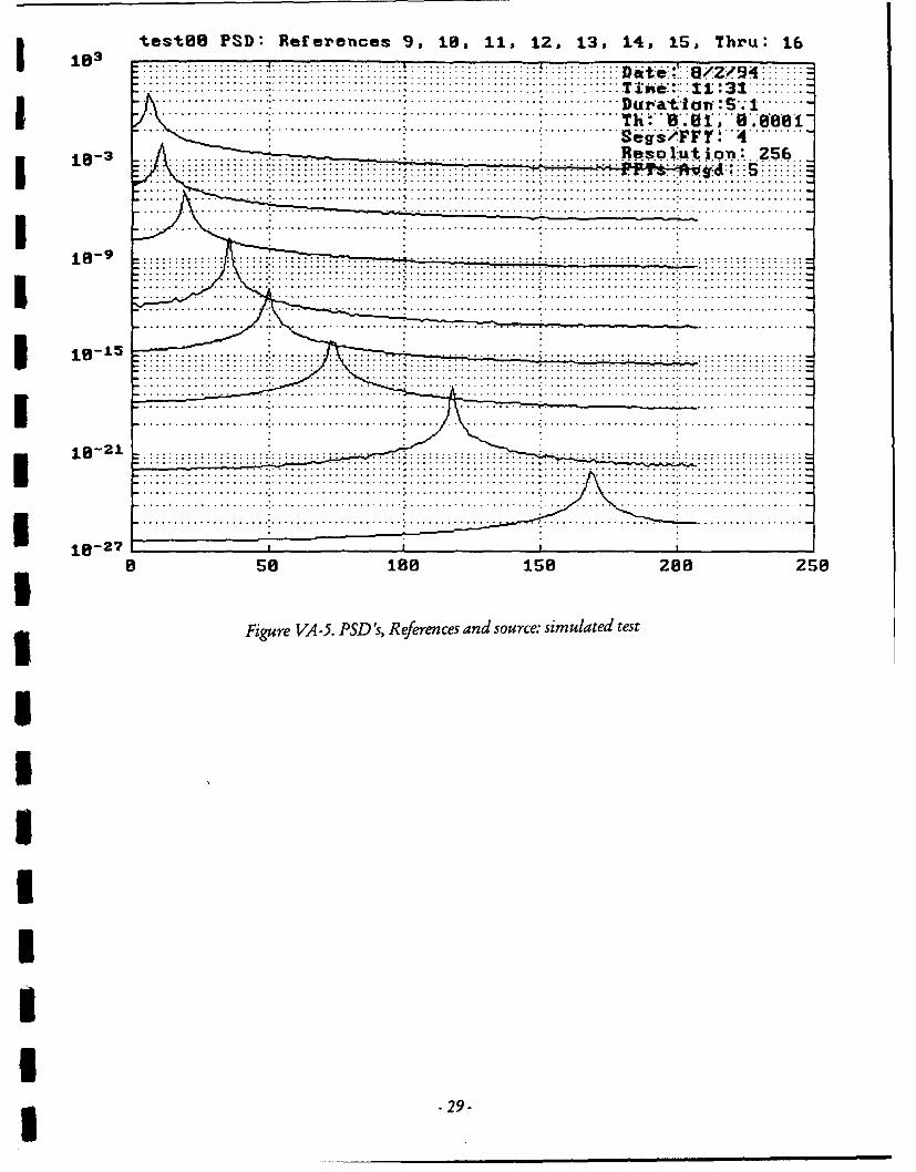
Figure VA-4 shows the coherence at resolution 256, of each reference with the source.Each of the 7 curves is plotted to a vertical scale from 0 to 1; the labels on the y-axis haveno other meaning. These coherences are all close to zero over the frequency band of

interest, suggesting that no substantial source energy entered the references. However, itshould be kept firmly in mind that for this particular example, the "coherences" are based

on deterministic time functions (sine waves), and therefore really have little if anymeaning. We would have been neither disappointed nor delighted had the plots come out

at something other than close to zero.

Figure VA-5 depicts the power spectral density (PSD) for each of the seven references (ch.9 - 16), and at the bottom, the source channel (16). The main subdivisions on the y-axisare separated by a factor of 10A6 or 60 dB; the absolute values on the y-scale, as well as theminor divisions, also have no significance.

2. Cancellation at resolution 512 and the relationship between resolution and optimal

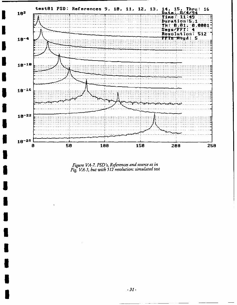
thresholds (test02.psd, test03.psd)

One of the noise cancellation parameters that has to be chosen is the desired resolution inthe frequency domain. This resolution, which we have normally set at 256, is the number

of source file time points used for an FFT. At resolution 256, the Nyquist frequencyoccurs at the 129th value in the frequency domain, so that the frequency range of interestis divided into 129 bins. Since the highest, or Nyquist, frequency is at half the decimated

sampling rate (2083/5/2 or 208 Hz, the width of a frequency bin for resolution 256 wouldbe 208/129 or 1.6 Hz. Resolutions of 512 (0.8 Hz) and 1024 (0.4 Hz) were also examinedbut seemed to offer little additional information and were more difficult to interpretvisually.

-36 .

Ui

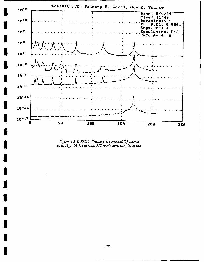
Figures VA-6 through 13 present an exploration the effect of frequency resolution. Figure

-a VA-6 shows the coherences of the 7 references with the source. These coherences came

out larger than when using resolution 256, but again, not too much heed should be paid

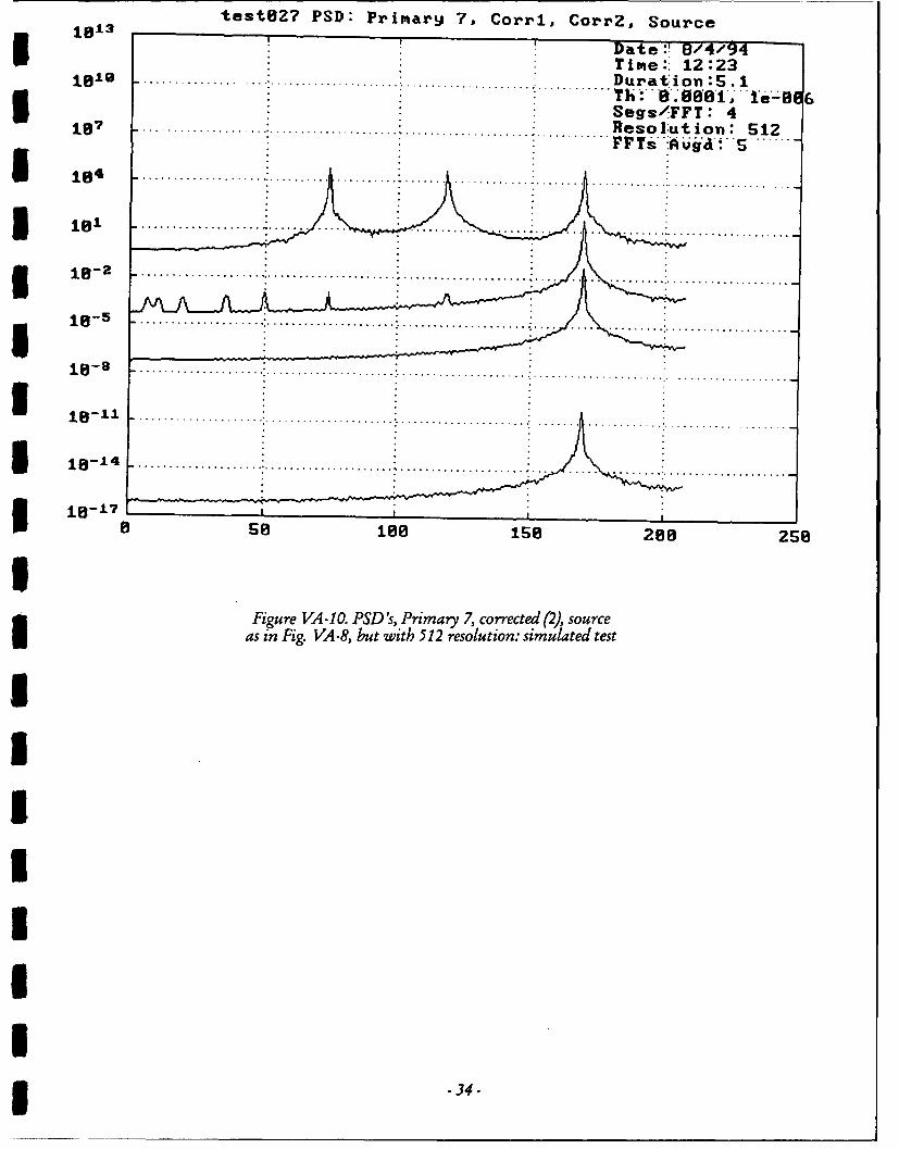
I to their values in the case of this deterministic problem. Figure VA-7 shows the referencepower spectra, which are similar to those corresponding to 256 resolution, except for the3 added jitter. The noise cancelling results for sensors 7 (Fig. VA-8) and 8 (Fig. VA-9)indicate that the thresholds of .01 and .0001 are not very suitable for this higher

resolution. Accordingly, the run was repeated with each threshold moved down some 20

dB. The coherences and reference PSD's are of course independent of threshold andtherefore identical to to those of Figures VA-6 and 7 respectively, but the noise cancelling

performance is improved as shown in Figures VA-10 and VA-11. This demonstrates the

inherent interdependence between effective resolutions and effective eigenvalue3t thresholds. This interaction between resolution and optimal thresholds has been

encountered before, and may be thought of as follows: When the bandwidth of the

Sfrequency bins is narrower, it is necessary to dig down relatively deeper into the set of

noise eigenvalues in order to obtain all those required for successful noise cancellation.

B. Sine Wave Input: 31 Hz source signal (a04555.psd, a04552.psd)

i We turn now to a closer examination of the successful example already cited at the

beginning of this Section V, when a 31 Hz sine wave was played by the loudspeaker. (In

i the test log, this source is reported as 25 Hz; the difference results from the fact that the

source was not calibrated, and this difference does not affect the validity of the analysis.)

But why, in particular, did the use of references have to be restricted to only 4 of the 7

available ones?

We begin with Figure VB-1, which shows all 16 channels recorded for this example: 8

primaries, 7 references, and the source. There are significant source harmonics at 62, 92,

123, and a small one at 154 Hz, which did not make it in a substantial way into anysensor, primary or reference. Figure VB-2 shows an attempted aoise cancellation using all

7 references with primary sensor 3 arbitrarily chosen for this study. The result is near

total cancellation of the source signal, regardless of which threshold was applied. Why?IFigure VB-3 depicts the power spectral densities of the seven references and the source.g The second, third, and fourth (References 10, 11, and 12 - the non-tailpipe microphones)

S- 37-

a84558 Channels 1 -16

kDuii1. es ton 2 56.

1I1 .. .%......

.. ...... .. .. ..... .. .. .

Io 1 ........ I -..

10 3 X-38..........

I a@45553 PSD: Primary 3, Corrn, Corr2, Source

1e20

Date:: 8/13/94

Tb: 0.01, 0.60081SSegs/.FFT: 4

.......I........ ... .... U lA ]eo Iit o'd;.'S'6-

UFsAvd1 8 2 ...... . ...... .......... ...... ...... .........

0 so 100 150 200 250

3 ~Figure VB-2. PSD 's, primary 3, corrected (2), source: 25 Hz sine wave

-39

I a84555 PSD: References 9, 18, 11, 12, 13, 14, 15, Thru: 16

... .: .... ..:: ,

1@................ .. ..... 4..tQ) 256.......

I 8~ ...... .................. ... .....

I. .................. ...... ....u ....j. . . . . . .. ... . . . .. . . . . . . . .. . . . ..2 I. .. . . . . .

... .. .... .8 18 15 288. 258........ ......

1I- Figur .B3 PSD. ...... Reerncsan suce 2 H inwv

I. ... .I. ............. ...I. .... ........ ......... ... ...: : :. ..........

IL -1... .. 40..

Ia64555 Coherence w. Thru: Refs 9, 10, 11, 12, 13, 14, 15

1 . Datesý 8/13/94

S.......................... ............................ .. "~.800iOOA................. Seg-s/FFT: 4I * Resol.U i'on: 256

-1 g:

-2 ......... .......... .. ........ .............

2I. ........................................... .........

-6 l iso 5 100 158 200 250

I Figure VB-4. Coherences of references with source.- 25 Hz sine wave

-41

1 a84555 Coherence, Refs w. Fet Ch. 3Date:! 8/13/94

S• iA . /• /'•i • . . fTime:': 13:S2

S. ......................... ................ . . ................................ . . .., .• , . .. .,e .. .e ..e e._B .• :. :SegsAFF 4,

SesFTesolution: 256S• ~ ~ ~ ~~Ts . g d . 5' ........

* -z...... .. .................... ............... ..........

I ....

442.

U a845522 PSD: Primarg 2, Corr,, Corr2, Source

_1 71 . . . . . . . . . . . . . . . . . . . . .. . . . . . . . . . . . . . . . . . I. . . .. . . . . . . . . . . . . . . . . . . . . .* . . . . . . . . . . . . . . . . . . . ... . . . . . . . . . . . . . . . . . . .

ie Date: 8/1/941811 iTime:: 14:583 . .................... e............... .... .................... ............ D U: i8i o i . : S .......Th: 0.01, 0.000tSegsý-,FFT : 4. . . ... . .. . . . . . . . . .. . . . . . . ... . . . . . . . . . . . Th . T

SFFTs :Avd: 5

1 80 2 . . . . . . . . . . . . . . . . . . . ... . . . . . . . . . . . . . . . . . . . . ,.. . . . . . . . . . . . . . . . . . . . . . . . . . . . . . . . . . . . . . . . . . . . . . . . . . . . . . . . . . . . . ..1_ 1 . . . . . . . . . . . . . . . . . . . ... . . . . . . . . . . . . . . . . . . . . •.. . . . . . . . . . . . . . . . . . . . . .. . . . . . . . . . . . . . . . . . . . . . .. . . .I . . . . . . . . . . . . .

S 1 8 _4 . . . . . I. . . . . . . . . . . . . ... . . . . . . . . . . . . . . . . . . ... :. . . . . . . . . . . . . . . . . . . . ... . . . . . . . . . . . . . . . . . . . . . . . . . . . . . . . . . . . .. .

I1B _? ....................

0 58 1t0 150 200 250

Figure VB-6. PSD's, Primary 2, corrected (2), source: 25 Hz sine wave

- 43-

I a845523 PSD: Primary 3, Corrn, Corr2, Sourcel8ea

1 3 1.7 . ......................................... . . . . . . . . . . ..................... . ....................

1 8 .@ .4 ..................... ................................................................ :. . . . . . . . . . .

Date:: 8/1/94*.......Time:: 14:58

l l .......................................... *................................. T i-m e ::i 14 ••:5 8 .. . .Th: 0.81, 8.8881

S............. . ............................... ...... SegsFeFT: 4

FFTs :Avgd: S

1 0 2, .................... ...................... * .................... i..................... -' .................... .-

1 0 - 4 .................... ..................... :.................. ...................... .......................

... . ..1. . . .. ..0. ....-.. . . . . .. . .. . . .. .. . .. ...................III

I 8 58e 18015 288 258

I ~Figure VB-7. PSD 's, Primary 3, corrected (2), source: 25 Hz sine wave

IIII

I .44-

I aS45524 PSD: Primargj 4. Cornl, Corr2, Source

* Date: 8/1/94lol ......... Time:: 14:58

Th: 8.01, 0.0001101 SegstFFT: 4

.. ... .. . ... .. t o.. .. .... .. .. ..... ...... ....

I LI so 5oo ISO1 200 250

I ~Figure VB-8. PSD 's, Primary 4, corrected (2), source:- 25 Hz sine wave

-45

a045525 PSD: Primarg 5, Corrl, Corr2, Source1029

II 8 4 . .................... ............... .. ............................................. :....................

Date" 8/1/94I O18 11 .................... ........................................................ TD im e ::' 14 :5 8'"t".. .. .IDuni~'f o*'n** .6 1'*

Th: 0.01, 0.0001Segst.FFT: 4JlOB 0} -:u .. .................. o.•o .. S'6' -

FTs Avgd: 5

I. ...1.............................................................. ..........................................

1 @ - 4 . ........................................ ........................ . . . . . . . . ....... ............. .

... ..... ............... ... ..... .. .. ..... ... . . . . . . . .

i0 s 100 15O 200 258

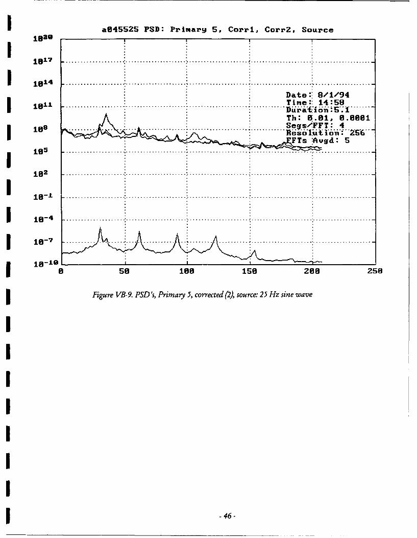
i Figure VB-9. PSD's, Primary 5, corrected (2), source: 25 Hz sine wave

-!IIIII

1 - 46-

I a845526 PSD: Primaz'g 6, Cornl, Corr2, Source

Date:* 8/1/94I ~....... ............................................ ..........Tiie 45

Th: 0.61, 6.0001SegsooFFT : 4I8 ........... : .2.. .. ....0. ...... ...............

FFTs :Augd: 5

.. .......... ........I. ... .................. ..

1021I oIO SO23 5

I Figure VB-f 0. PSD's, Primiry 6, corrected (2), source.- 25 Hz sine wave

-47

I a845527 PSD: Primary 7, CornI, Corr2, Source

I . Date:: 8/1/94

Th: 6.0i, 0.ee01too ... .. ......... Segss/FFT: 4I ~Resolution: 5256

.. .......... ...................I. .. ........... .........

I0 so too 1S0 208 258

Figure VB- 11. PSD's, Primary 7, co rrected (2), source:- 25 Hz sine wave

-48

I a845528 PSD: Primary 8, Corrl, Corr2, Source

is'?I 81is14 . . . . . . . . . . . . . . . . . . . . . . . . . . . . . . . . ...............................

Date:: 8/1/94Tine:: 14:58t l .................... ............ ............................... ............... -'........... '5. i* .. . .

nurtion:S.1.i Th: 8.81, s.8081: Segs/.'FFT: 4

.Resolut ion 256: FFTs : gd: 5

1 0 5 . ............................................................. ... .................................. ....... .

I 1_

I 1_

i7. .......... .................... ....... .........1j-18 |

8 58 188 158 288 258

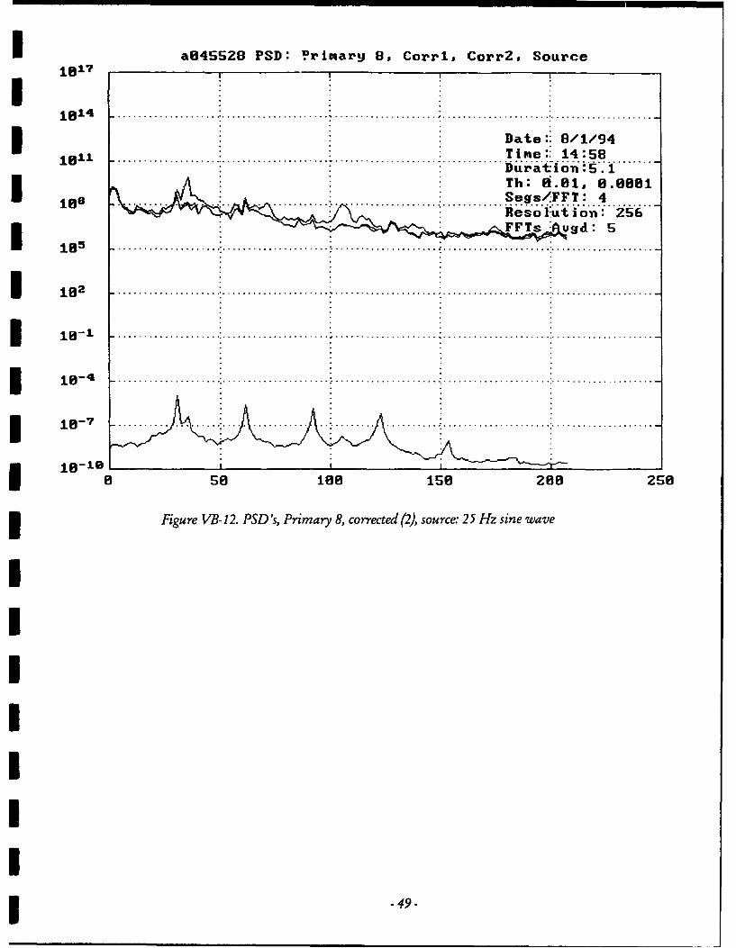
Figure VB-12. PSD's, Primary 8, corrected (2), source: 25 Hz sine wave

- 49.

I

show substantial peaks at the several source frequencies, while neither the tailpipe

microphone nor the three accelerometers exhibit this phenomenon.

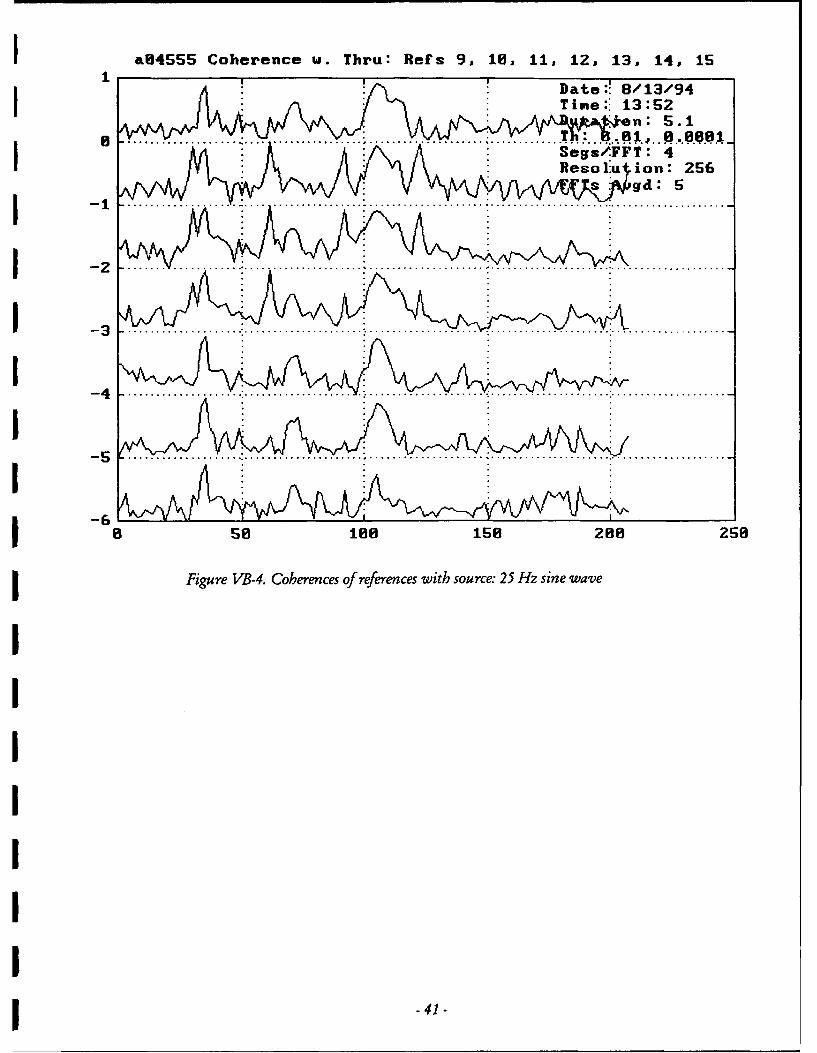
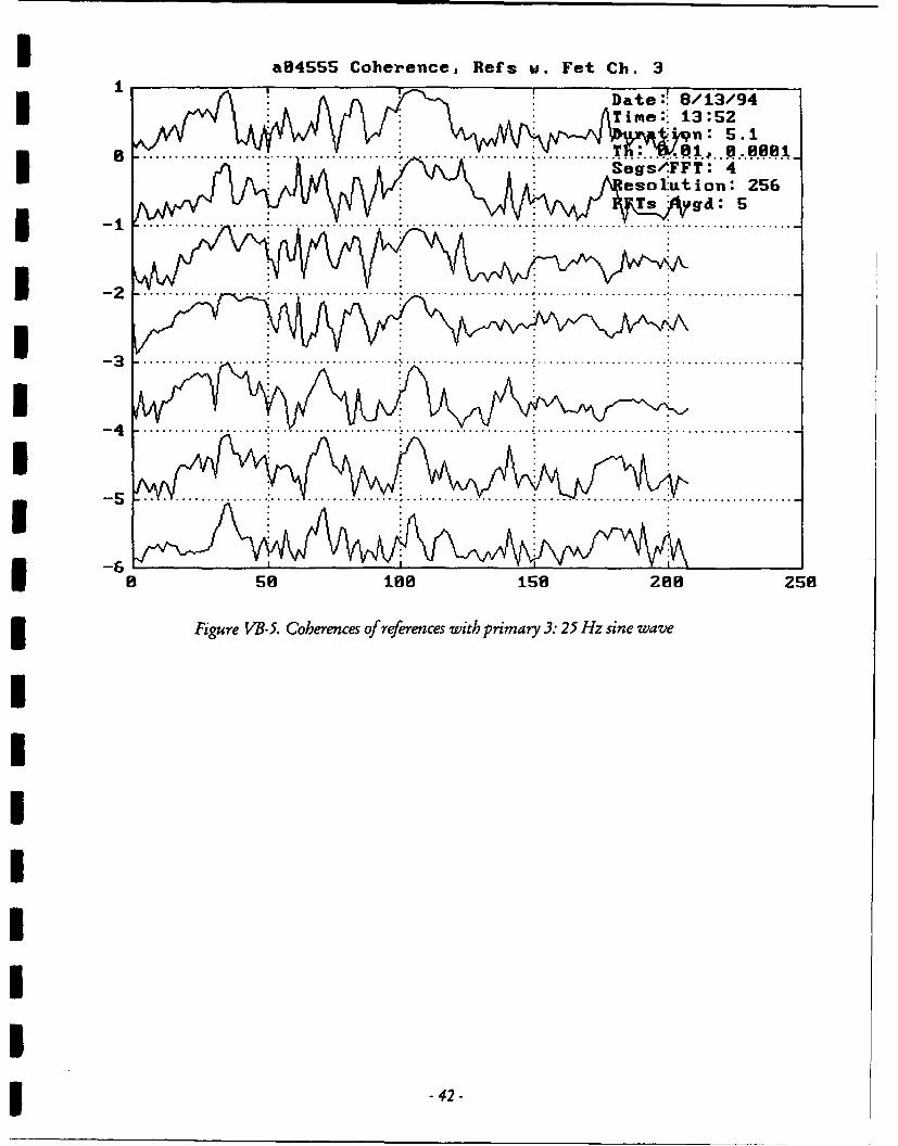
Finally - and importantly - the coherence function of each reference with the source (Fig.

VB-4) shows that the offending signal peaks in the reference power spectral densities infact represented energy coherent with the source ("Thru" channel). Is coherence

"transitive?" It is, somewhat, as indicated in Figure VB-5 showing the reference coherenceswith primary channel 3 instead. The same peaks do appear in these coherences as do in

those taken w;th respect to the source itself.

Thus, the indicated solution in this experimental example was to omit the offending

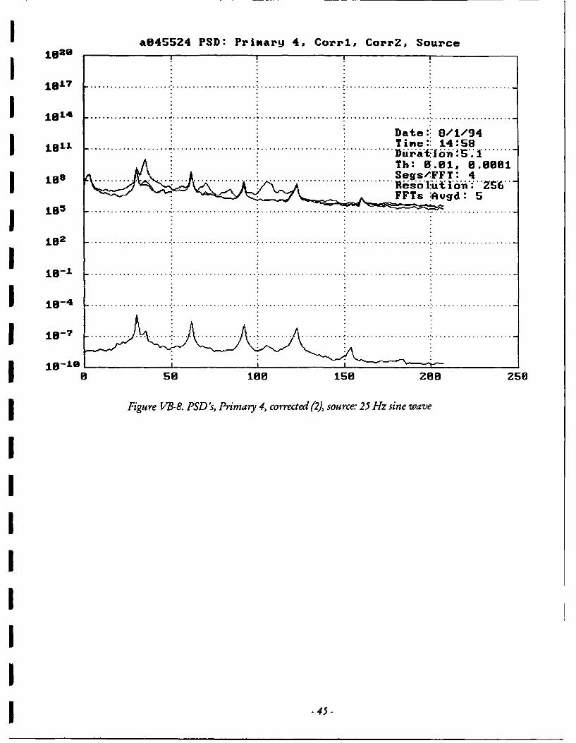
reference microphones and to only use the tailpipe microphone and the threeaccelerometers. The results for Primary 1 has already been shown in Figures V-1 and V-2;

results for the remaining primaries (2-8) are shown in Figures VB-6 through 12, in

overlaid fashion for easy visual interpretation of engine noise actually cancelled. Results

for all four primary microphones facing the loudspeaker are very similar; the four on the

far side show that the signal did not reach them very well. Primary microphones should,

if possible, be mounted standing up from the roof rather than on the side of the vehicle,

in order to provide more nearly omnidirectional sensitivity.

C. Simulated Vehicle Drive Bys - 1

A number of vehicle driveby recordings were analyzed. Little effective noise cancellation

with signal retention was produced in any runs that we examined, because of the

relatively large amount of signal source energy entering each reference. There were no

good, i.e, sufficiently "signal-free," references eligible to provide noise cancellation, as wasthe case in the above illustrated test case and the sine wave recording.

To solve this problem, a more fully instrumented test should be held, in order to

optimize the types and locations of the sensors, and most especially of the reference

sensors. In such a test, the spectrum of all sensor responses to the source, as well as to theengine, should be measured. In addition, the coherence between the source and any

sensor, and the coherence between pairs of sensors, should be measurable on the spot.

* Reference sensors should pick up the largest obtainable levels of engine noise so that their

gains can be set low enough to exclude most of the signal from the loudspeakeres. All

* reasonable reference sensor location should be tested: in or on the exhaust system but

I 50-

a11400 Channels 1 - 16U 1012I I

Date:: 8/13/94DurationS51l

t o o .... .. .. .. ... .. .. .. ... .. .. .. ... .. .. ... ... ... .. .. .. .. .. .. .. ..Io: 5

I6 .................... ........ .........

.. .................*. .... ......I. ........ ...................... .........

I0 2 ..... .... ...... ....... .........

10-421-58s 108 158 288 250

I Figure VC-1. PSD's of all 16 channels:- M60 tank, 15 km/hr

1 -51-

I a114923 PSD: Primary 3, Corrn, Corr2, Source

............. .................................. .......

IDate:: 8/13/94

Duratioii:5.1I Tb: 0.6i, 8.8801Segs/-FFT: 4Resolution: 256,

.. ... F.... -A g :

Ieou... ...I. ... ....... ................

I L0 .......... ..

JLB-91 so5 160 ISO 2100 258

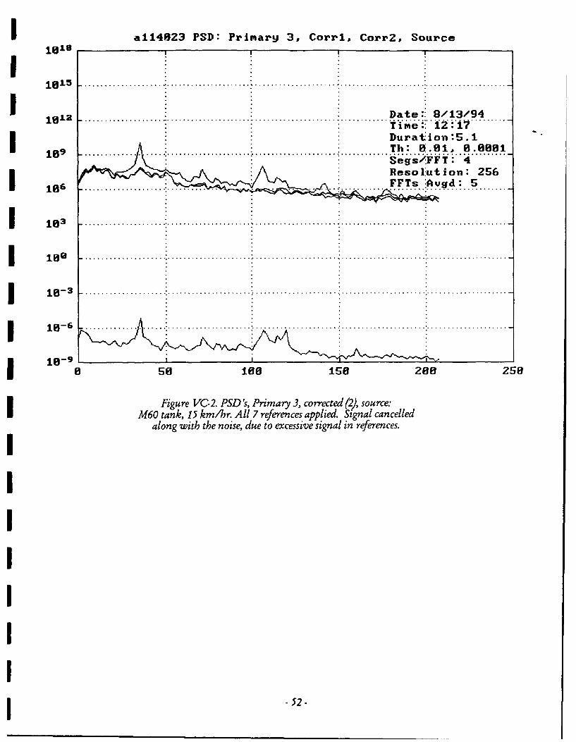
Figur VC-2. PSD 's, Primary 3, corrected (2), source.-

M0tank, 15 km/hr. All 7 references applied. Signal cancelledalong with the noise, due to excessive signal in references.

-52

I a114863 PSD: Primarg 3, Corrl, Corr2, SourceIsis

1 ±1 5 . .......................................... ..............................................................

S.......................................................................D.t.. 8 / 13 /. .Time:: iz.....Duration:5.iU................. ..01, 0.0001

I 6 9O .. ....... .... ... .i............................................. .. ... .... .............. i• : 'I~i i • • ..........-.'Se:s/.FFT: 4

Resoliution: 256

1 0 6 . ................ ..... ... .......... :.. . . ... . .FF T s.:. .gd : .

I L136 ...................... ........... ..................... ....................

1 3 . ... .. .. . .. .. .. ..... .. ... ...... ..... .. ... .. ... . .. ... .... .. .. . . ........ . .. ... .. .. . ... .. . ... .. .. . . . .

IL1 -0 . . .. . .. . . . .. .. .. .. ..... ......... . I.. ... ..... . .. ... .. .. ..... .... . .... .. .... .. .. .. .... ... . .. ........ ... ....

I L 6 . ... .. .. . .. .. .. .. ... ... .. ..... .... .. ... ... .. ... . .... . .. .... ..... . . ..... .. ... .. . . . ... ... ........... . .

S 10-9

U8 50 100 158 288 258

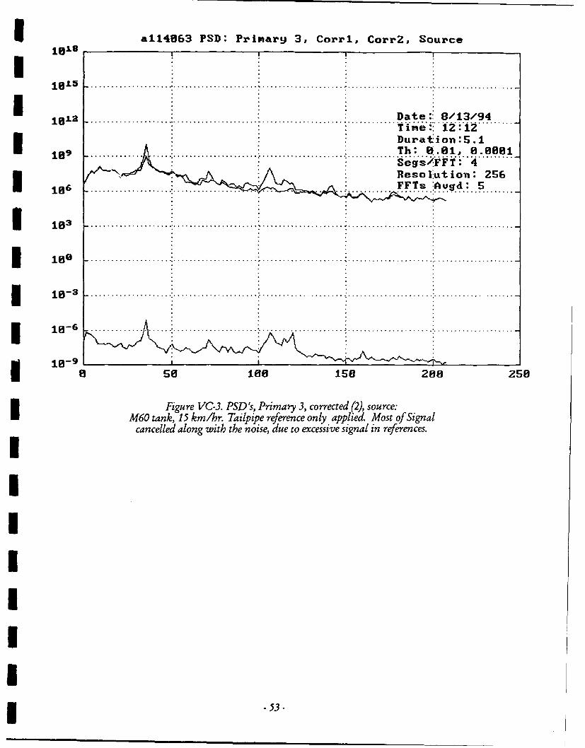
i0 Figure VC-3. PSD's, Prima•y 3, corrected (2), source:

M160 tank, 15 km/br. Tailpipe reference only applied. Most of Signalcancelled along with the noise, due to excessive signal in references.

I

-I3

&1142Z PSD: References 9, 18. 11, 12, 13, 14, 15, I Tru: 16tl e.. . .. . ........ • . . . . . ..... L .......... .. . . .................... . . ... .. ... .

....... . ......

.. ...... ................ ...... ..... ......

....... . . . . . ... . ... ." .......... . D a t e.:: 1 / 94 . ......

Time::* 17:415 .....

"..". .. Dur.ation;s.1 ..

.............. ,.:...

........ .. .. " -................... . . . .. ......4 .t e • . ....... ........... ............ . .. ..--• : :: .. ... ... ....... • :i -: • : 7 :

I........ .... ..•:... ...

..... ..... -... -.............

....... .

. ..I i... ........

................ ................. .......

. .......

I" _z :-• " . ... .. : :: :: : . .. .....-• i . ....: : : :. : .i .................... ................. -.

"I- .. .... "• ........ . .. .I, % l" / , .-.---... .. . . - ,. . . . .

I. ........ ............I ........I 2. ..... e

.. . . . . . . . . . . .. . . . '...... . . . . . .. . . . . . . . . . . . . . . . . . .. . . . . . . . .. .. . . . . .. . . . . . . . . . . .. . . . ..... . . . . . . .. .. . . . . . . . . .. . . . .. . . ... ..... -... ... .. • '.... . . . . . . . . .

.. . . ... . . . . . . . . . ... . .. . . .• .. . . . .. . . . .. . .. . .. .• . . . . . . . . .. . . . . . . .- .. . . . . . . . . . .. . . . . . . . .... . . . . . . . .. . .. . . . -

S.. .. .. . . .. . . . . .• . . .. . . . . . .. . .. . . . .. . .; . . .. . . . .. . . . .. . . . ... • .. . . . . . . . . . .. . . . . . . .. . . .. . . . . . . . . .. . . . ..

II .... ..... : .... : . . . .... ... . . ... .. .. .. ... .. .. ... ..u

I

ISO'5818 158I 200 2S8B

IFigure VC-4. PSD's, References and source: M60 tank, 15 km/br

II.I

II

! - 54.

I a11482 Coherence, Refs w. Thru Chi. 16

1 Date:: 8/13/94

Segs/FFT: 4

Re ol~u ion: 256T gd.. .... ..-2. .. ...... .... ....

12 ........... ............

I0 58100 ISO 200 256

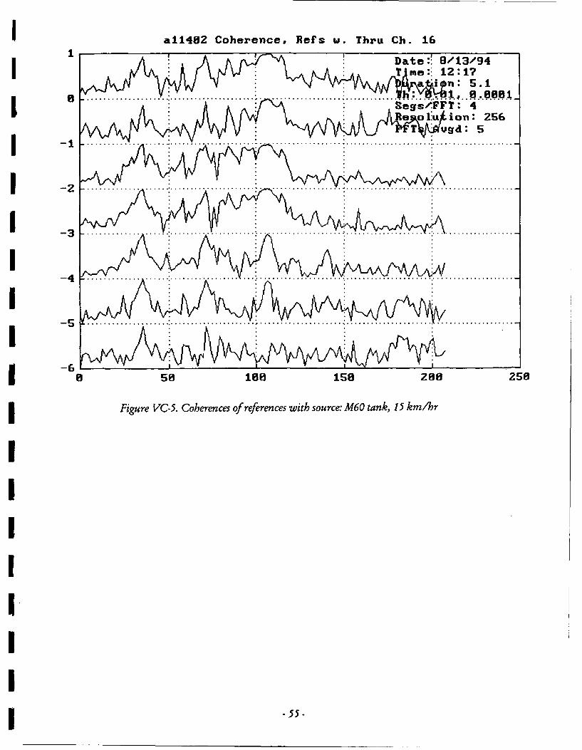
I ~Figure VC-5. Coherences of references with source: M60 tank, 15 km/hr

-55

closer to the engine, at locations on the engine block or on the engine head, to mention

just a few. These may well be accelerometers rather than microphones. The present

location of the tailpipe microphone happens to have been on the side of the vehicle nearthe tailpipe and away from the loudspeakers; if the loudspeaker source were instead onthe same side of the vehicle as the tailpipe, then the tailpipe microphone would probablyreceive even more loudspeaker signal than it does now. If omnidirectional response isdesired for beamforming, then the primary microphones should stand up from the roof.There are lots of ideas - but they need to be tested.

Moreover, since nearfield source effects are unpredictable, the speakers should be placedsufficiently far away so that the vehicle will be in their far field. For example at 20 Hz, awave length in air would be close to 60 feet away. All source levels and signal as well asnoise levels received by the sensors should be carefully monitored and logged, and the

noise sensor locations should be adjusted for best likely performance.

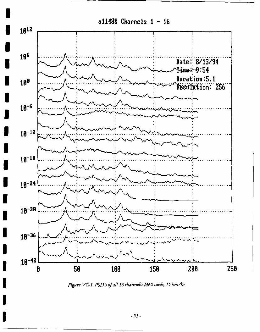
I Files a11400, a11402, and a11406 playing the driveby of an M60 tank travelling at 15km/hr present as good an example as any other. Figure VC-1 shows the power spectraldensitities of all 16 channels (8 primary, 7 reference, and the source) for a 5.1 second

record 19 minutes (1140 seconds) into Tape 1 or a. Figure VC-2 depicts in overlay fashionan attempt to cancel the noise in a typical primary sensor, in this case number 3, using all7 references. Clearly lots of noise gets cancelled, but so does most of the signal. FigureVC-3 shows the slightly better but still very poor result when only the tailpipemicrophone is utilized as a reference. Here, of the signal appearing in the uncorrected

version at about 35 Hz, some 12 dB of it is thrown out by the cancelling process. A bit

better than using all references, but not much. On the other hand, the all-references casedoes cancel considerably more noise than just the tailpipe microphone alone. Why andwhat to do?

Again the answer to the question lies in careful examination of the reference psd's and

I coherences with the source. Such examination reveals that all references have strong andcoherent energy at the source signal peaks. It is a clear case of too much signal in theI references - all of them, and their correct positions must be determined experimentally.

5

I.- .56 -

ID. Simulated Vehicle Drive Bys - 2

It has been noted that Tape 5 was done with the HMMWV's engine turned off, and was

therefore of somewhat lesser interest in connection with the present study. However, weI wish to cite an example from it. We do this in part because this case at first caused usgreat concern about the correctness our software, until we found out what was

j happening. More importantly, this example dramatically illustrates the value in noise

cancelling of examining coherences as well as power spectral densities of sensors.

I Figure VD-1 depicts all 16 channels for Run e11400, some 1140 seconds into Tape 5 (or e).

Again, we meet our old friend the M60 tank travelling 15 km/hr, but this time with the

HMMWV's own engine turned off. Our concern in this run was with the prominent

peak at 80 Hz. Since this peak does not appear on the last curve, the source spectrum, its

I real origin is not known with certainty because the recorded version of the source

contains almost entirely what appears to be 60 Hz hum and its harmonics at 120 and 180

Hz. Thus, the recorded version of channel 16 did not correspond to what the

loudspeakers appeared to have actually put out.

In any case, the attempted noise cancellation shown in Fig. VD-2 exhibits a blatant and

stubborn refusal to cancel that 80 Hz peak, even though it shows up in force in the first

four references, the reference microphones. As advertised, the coherence picture solves

the puzzle. Figures VD-3 and 4 prove that whatever acoustic energy appears in the

reference sensors at 80 Hz has a coherence of no more than 0.5 with either the recorded

source (Fig. VD-3) or with Primary sensor 1 microphone itself (Fig. VD-4).

In this connection, it may be useful to review just what any given coherence ought to do

for noise (or signal) cancellation. While this problem is complex for a multi-channelsystem, the relationship is straightforward for the special case of a single reference: The

I gain achievable against noise by such a reference is simply

Gain - - 10 log10 (1-r2),Iwhere r is the primary-reference coherence (square root form as plotted in our graphs).

I Thus, a single reference having a coherence of 0.5 with a primary channel could not have

removed more than 1.25 dB of the signal or noise in question.

I• .57-

Ie11400 Channels 1 -16

ITime:: 0:25

Resol~ution: 256

.I ................... ........

to ............... . ................ ........... ......

1I1 ............................................

Io. ................% ....................

5 188 158IS 208 258

IFi re VD-1. 16 channels: M60 tank, 15km/hbr, own enginn e off.2Nte peak at 80 Hz in first 4 primaries and in first 4 references

I .58 .

I e114881 PSD: Primary 1, CornI, Corr2, Source

*....Date:: 8/7/94

Tine:: 280:27

.. .. .. .. .. .. .. ... .. .. .. .. .. .... .. .. .Durat ion :5

Segs/-FFT: 4............. .... .... Resolution: 256

..... ........... ....1 8I. .................. ..................

I 8so 188 158 288 258

I Figure VD-2. Failure to cancel peak at 80 Hz:-M60 tank, J5krn/hr, own engine off

-59

e11400 Coherence: References 9, 10, 11, 12, 13, 14, 15

*Date:: 8/7/94

. ........... z ............. ..... .. ......... .*.* Segso"FFT: 4* Resol~ution: 256

I-FýsII

.. ............. .................. .......... ..... ....-25 ........... ...

-60 50 too 1s@ 200 2S8

I Figure VD-3. Coherence of all 7 references with the source.

- 60.

1 ~e114OO Coherence, Refs w. Fet Ch. 1I/29

D Date **.1

T m.I ......

-3 1:2

I~~~~- 0d 501010 0 5

IIVIIIVP

3I. .......................... ..........................

-4 ............ ........... ........... ........... .........

I *-61-

VI. Conclusions

1. The experiments and analysis that have been performed have shown that the enginenoise getting into the signal microphones of the test vehicle is readily cancelled.

2. The signal was received well on the side of the vehicle facing the loudspeakers, butmore faintly on the far side. If omnidirectional sensor reception is desired for effectivebeamforming, the primary microphones should probably stand off the roof rather thanbe mounted on the side of the vehicle.

3. The signal has been preserved in some cases, but in most cases, its strong and coherententrance into all references prevented signal retention as the noise was cancelled. Becauseof the particular coherences involved in the process, signal retention happened to be quitegood for the 31 Hz tone, but poor for all the drivebys which were studied.

4. The noise sensor power spectral density (PSD) plots of the noise or reference sensorsshow that all these references have significant peaks of sound energy at precisely the

frequencies at which the loudspeaker source had major peaks. This strongly suggestedthat significant loudspeaker signal was getting into each reference sensor.

5. The coherences plotted between each reference sensor and the source itself confirms the

conclusion stated in 4: The PSD peaks appearing in the noise sensors at source frequenciesdo represent energy that is in fact coherent with the source energy at those frequencies,and should therefore be expected to be cancelled along with the noise.

6. When the data was taken, the greatest concern was to be sure to get the signal into thesignal microphones. This has turned out not to be a problem at all; the problem to be

solved is to not get too much of it into the noise sensors.

7. Judicious choice and location of noise sensors should remedy the above stated

difficulty. Accelerometers would in general pick up less source signal than microphones.Locations to be considered would include further up the exhaust system, near the exhaust

manifold, at various sites on the engine block and head, to mention a few. A tachometeron the engine, and a capability to produce the harmonics of the tachometer as possible

reference inputs, could be useful. This technique has been used extensively in the active

.62-

cancellation of engine noise in aircraft cabins. A new test should include the capability to

measure spectra as well as coherences for all sensors and sensor types, and sensor positionsshould be selectable during the tests.

8. In a new test series, more attention should be paid to getting a measure of absolute

levels of signals and noise received by the various sensors, especially the noise sensors, and

independently from either the engine or the source loudspeakers. The placement of the

noise sensors should be adjusted experimentally in order to minimize the signal at their

outputs. Also, in a new test, data file lengths should be kept a little more manageable: In

the tests which have been concluded, each tape contained a single file pair which, when

loaded into an IBM compatible computer, uses up the bulk of its entire disk space. The

engine should be tested at a variety of speeds in addition to idling.

I 9. Assuming that appropriate noise sensor types and locations can be found to remove the

above stated difficulties from the signal and noise measurements, the development of a

I real-time online noise canceller based on these principles would be well within existing

technology, built primarily form commercial off-the-shelf (COTS) components.

6IIIIII

I

I' VII. Recommendations

1 1. Perform another test series on the HMMWV vehicle, with appropriate spectrum and 2-

channel coherence measurement capabilities, and with a wide selection of candidateI reference sensor types and locations. The main purpose of such a new test will be to

optimize the sensor configuration, especially the reference sensors. The test should be

I planned for at least two days rather than only one, in order to allow some off-line analysis

of results before completing the series. The specific recommendations for such a newI tests are listed in the following separate Section VIII.

2. Complete work on an adaptive code version making use of the Lockheed-Sanders data

formats. Make the single-pass and adaptive codes more efficient and determine

requirements for a digital signal processing board and other computer components toI develop a real time multi-channel noise canceller.

1 3. Develop a real-time multi-channel noise canceller. Such a device would be useful also in

other Army applications. Possible examples are noise-limited hand held endfire acoustic

detection arrays under development at the Army Research Laboratories in Adelphi, MD,

and an acoustic sensor project underway at the Army's Night Vision Electronic Sensors

Directorate at Ft. Belvoir. Additionally, the development of a realtime multi-channel

noise canceller would present a significant opportunity for technology transfer to

commercial applications. Medical instrumentation, quieting aircraft cabins, and

I applications in the communications industry are likely candidates to welcome such adevelopment.I

I VIII. Specific Recommendations for New Test Series

The new tests recommended as item 1 in Section VII above should be planned as follows:

1. The main purpose of new tests is to determine the best sensor types and locations,I especially for the reference sensors.

1 2. Sensor types and positions should be changeable during the test.

I1 -64 -

I

3. Instrumentation should be available for the measurement of power spectral densities of

all sensors, as well as the coherence between any two chosen sensors.

4. Reception of loudspeaker signal and engine self noise by all sensors should bemonitored and relevant coherences examined, especially coherences between thereferences and the source.

5. Nonlinearities in the system should be minimized. In particular, the source should beI placed far enough away to put the vehicle in its far field.

6. The primary sensors should stand off from the roof, rather than be mounted on the

side of the vehicle.

1 7. Candidate reference sensor positions should include, but not be limited to, further upthe tailpipe, mounted at various locations on the engine block and head, near the exhaust

Smanifold, etc. The object is to get maximum noise level so the gain can be turned downenough to reject most of the signal.

1 8. More accelerometers should be tried, rather than reference microphones.

I 9. Any tailpipe sensor microphone should not be mounted on the side of the vehicle. Itreceived signal there during the tests, and would have received more of it had the sourceI been located on the same side of the vehicle as its tailpipe.

1 10. Primary sensor microphones should be mounted on vibration isolators to minimizenoise getting into them.

1 11. Reference sensors should be isolated as much as possible from signal, not only through

choice and location of the sensors but also through the judicious use of passive acousticdamping materials.

1 12. The engine should be operated at a larger selection of speeds, not only at idling.

13. The tests should be planned for at least two days rather than only one, to permit some

offline analysis of the data before completion of the series.

II 65-

Appendix A: Codes Used in the Calculations

1. System for naming data files

This section is presented primarily to facilitate reading the filenames printed on the title

line in each plot. File types are identified by the file extensions .gl, .g2, .ecg, .fcg. of .psdas defined below. All plots are prepared from groups of ".psd" files.

1. .gl, .g2 files: These files are the original data files generated by Lockheed Sanders, Inc.test equipment and named by Lockheed Sanders personnel. These files are read by

readlock.for to prepare an .ecg file for subsequent analysis. The files come in pairs .gl and.g2 , with .gl containing eight channels of primary sensor data, and .g2 containing 7

channels of noise reference data and one through channel recording the loudspeaker

source input. The sampling rate has been set at 2083.3 Hz. These files are long, about 45

Mbytes each, making them a bit unwieldy for use on a PC.

2. .ecg files: This is the original data, low-pass filtered and decimated by a factor of

approximately 5 to yield 16 channels of data with a Nyquist cutoff frequency of 1/10 the

sampling rate or 208.3 Hz. A synthetic .ecg file can be generated by program testfll.for.A typical .ecg filename is 'a0455200.ecg.' This name identifies the run generating it asI follows: The first digit, 'a', refers to the first of 5 data tapes. The next four digits '0455'denote the time in seconds from the beginning of the tape, according to the test log

Sshown in Section V. Thus, '0455' means 455 seconds or 7 minutes and 35 seconds into

Tape a, at about the middle of a 25 Hz sine wave recording. The sixth digit is also

assigned to the .ecg file, but may be modified when the parameters used in the noisecancellation calculation are varied from their default values. A fifth digit other than "0" in

the .ecg filename is used when readlock produces an .ecg file using other than the"standard" 5.1 second interval. A When .psd files are formed, the last two digits of the.ecg filename are overwritten as described below.

3. .fcg files: Normally used in electrocardiography and other applications where time

I domain information is required. Not used in this report.

I 4. .psd files: Power spectral density of reference sensors, source signal, primary sensors,and corrected primary sensors; coherence between each reference sensor and the source

signal.

I 66-

II

The last two digits of the file name pertain to the particular information in the file. If thee initial digits of the .ecg filename are followed by an 'i,' the file is an information file

used to write a title and other information on the plot. A single numeric digit (7th of a 7

I digit filename) refers to the number of a primary sensor from 1 to 8. A single digit

followed by 'r' as the eighth digit refers to one of seven reference sensors; 'lt' refers to the

I through or signal channel; while a single (reference sensor) digit followed by a 'c' refers to

the coherence between the reference sensor and the signal input. Channels containing

I corrected primary data have as their 7th digit the number of the corrected primary

channel, while the 8th digit denotes which of two thresholds was applied to the

eigenvalues. The generally used default value of these thresholds were 20 and 40 dB

respectively below the largest noise eigenvalue.

2. testfll.for: Generation of synthetic data file to test calculation programs.

This program was written to verify the correctness of the noise cancellation calculations

performed by armsp.for. Each of 7 simulated reference sensor signals (multiplexed

channels 9 through 15) consisted of a single sine wave, each of a different frequency,

whereas the 8 primary sensors were represented by various linear combinations of these

reference signals. The "through" or "source" signal was taken as still another sine wave.

The output format is identical to that of an .ecg file produced by readlock.for for real

data.

3. readlock.for: Reading, low-pass filtering, and decimation of data files generated by

Lockheed Sanders, Inc. test equipment

This program reads the two original data files (.gl and g2), and performs the followingfunctions on the data:m- The data is normalized to assure that each reference channel is given approximately the

same weight in the calculations;

P- A 128 point convolution filter is applied to filter out all except the lowest 20% of the

frequencies contained in the original data, yielding a Nyquist cutoff frequency of 20% of

half the 2083.3 sampling rate or 208.3 Hz.

P- The data is decimated by a factor of 5, providing a new "sampling rate" of 416.7 Hz.

67-

- The data is recorded in multiplexed fashion in the resulting .ecg file.

4. psd5.m, titl2.m: Plot power spectral densities and coherence

This code uses information from a collection of power-spectral density and related .psd

files to generate the plots presented in this report. The numbers in the filenames pertain

to the most recent version of the program. These programs require the use of Matlab for

execution.

The code for performing the actual noise cancellation consists of code developed using

private funds for the study of fetal electrocardiography, modified to accept the Lockheed

Sanders, Inc. data format. This code is submitted to the Government as a proprietary

addendum.

- 68 -

"c readlock.for rev jcs: read as direct files"c readlock.for rev jcs; 940710 fr - formatting; fix write(31,); sampFreq"c readlock.for rev 940415 fr: rewind, nStatPoints"c readlock.for 940402 cs made points correspond to old calculated vals."c readlock.for 940331 csfr (fix write to rec=6, reduced screen print)c"c This is a simple program to read the data files from Lockheed Sanders."o The data is in two byte signed integer format. Output is a standard"c .ecg file, but with 16 channels.c"o J. Clarke Stevens"c Signal Separation Technologies"c Feb 22, 1994. Long Live George Washington!cc Main program block:c

program ReadLockcc Set constants:c

parameter (frequency = 2083.333333) undecmtd sample frequencyparameter (nChannels = 16) number of channels, 2 infiles

c parameter (nChannels = 8) I number of channels, 2 infilesparameter (nChannelsPerFile 8) ! number of channels per fileparameter (numWeights = 129) ! number of filter weights

c parameter (nPoints = 250880) 1 number of points per channelc parameter (nPoints = 2000) 1 number of points per channelc parameter (nDataStart = 100) ! position for data startc parameter (nStatStart = 200)c parameter (nDataStart = 3000) ! position for data startc parameter (nStatStart = 3000)c parameter (nStatPoints = nPoints - nStatStart) ! points for stats

parameter (iDecimator = 5) ! decimation factorc

character*2 versfnmcharacter*6 genfnmcharacter*12 lokfname(2), ecgfname ! 2 input files and 1 .ecg fileinteger*2 idataPoint(nChannels,numWeights) ! array stores datainteger*2 iData ! point for calc of norminteger*4 i ! loop index counterinteger*4 iPoint ! current pointinteger*4 iPosition I position for point in arrayinteger*4 iChannel ! current channelinteger*4 iWeight current filter weightinteger*2 iNormalChannel ! normalization reference chaninteger*4 nStatPoints I number of points for statsinteger*4 nPoints ! length of interval in pointsinteger*4 nDataStart I start position of datainteger*4 nStatStart I start position of statsreal*4 channelMean(nChannels) ! mean vectorreal*4 channelRMS(nChannels) RMS vectorreal*4 channelFactor(nChannels) ! normalization vectorreal*4 channelData(nChannels) I data from filereal*4 referenceFactor ! normalization referencereal*4 filter(numWeights) ! the filterreal*4 filteredValue I value of new filtered pointreal*4 outputArray(nChannels) ! filtered data

cc Initialize the filter:c

DATA filter / ! fir2(128, 0.2)"* -0.00006034715814, -0.00009941091517, -0.00012253653140,"* -0.00012028676864, -0.00009242607391, -0.00004830372057,"* -0.00000372571763, 0.00002516793517, 0.00002896915489,* 0.00000982576943, -0.00001893206551, -0.00003926645345,

- 69 -

* -0.00003863192636, -0.00001866189178, 0.00000340052880,* 0.00000334184665, -0.00003407792675, -0.00010018672209,* -0.00015880652690, -0.00016051815368, -0.00007217562514,* 0.00009142335120, 0.00025274476980, 0.00028910272145,* 0.00008429697520, -0.00040324181965, -0.00108862727079,* -0.00175946196572, -0.00214313945983, -0.00202871289202,* -0.00139646475704, -0.00049056576074, 0.00021892251965,* 0.00019721237613, -0.00091662052100, -0.00308955168638,* -0.00580425027097, -0.00817446923883, -0.00926214962530,* -0.00849584334273, -0.00601968361042, -0.00279632750809,* -0.00036200983333, -0.00026871329733, -0.00339705574340,*-0.00941878856097, -0.01667716091679, -0.02262234188681,* -0.02472390264145, -0.02156211412970, -0.01366835750137,* -0.00371252253126, 0.00416483462586, 0.00576261007593,* -0.00145935733668, -0.01697073075788, -0.03666996979762,* -0.05362766771134, -0.05998681105141, -0.04949498879655,* -0.01985468869073, 0.02594069073519, 0.07983730167155,* 0.13057277352257, 0.16665732094943, 0.17958793692696,* 0.16628817069530, 0.12999470587605, 0.07930730576657,* 0.02571109266601, -0.01963496700252, -0.04883733502557,* -0.05905609841986, -0.05267563950488, -0.03593652815811,* -0.01659290857436, -0.00142354365837, 0.00560796483330,* 0.00404342501426, -0.00359562105677, -0.01320568141090,"* -0.02078073134310, -0.02376816501575, -0.02169243184358,"* -0.01595021289488, -0.00898448963124, -0.00323172193383,"* -0.00025493587607, -0.00034249065892, -0.00263801670633,"* -0.00566235833030, -0.00796775203712, -0.00865997387457,"* -0.00761917668506, -0.00539268295469, -0.00286107650384,"* -0.00084598415796, 0.00018138751069, 0.00020064334689,"* -0.00044797321677, -0.00127046810934, -0.00183861716398,"* -0.00193471072745, -0.00158197279847, -0.00097479230527,"* -0.00035956320142, 0.00007484553011, 0.00025557837650,* 0.00022246161379, 0.00008011732734, -0.00006297506050,* -0.00013945872498, -0.00013740345923, -0.00008634753125,* -0.00002926680768, 0.00000286131625, 0.00000290466756,* -0.00001591721593, -0.00003294034542, -0.00003352141111,* -0.00001621158932, 0.00000845869992, 0.00002513869422,* 0.00002208248157, -0.00000331626737, -0.00004376782194,* -0.00008553486229, -0.00011402362221, -0.00011923516930/

c DATA filter / ! firl(32, 0.18)c * 0.00058458747668, 0.00152178621646, 0.00260408350366,c * 0.00337243944497, 0.00273793424247, -0.00051567165154,c * -0.00679459801153, -0.01477347432336, -0.02105847894341,c * -0.02082849374397, -0.00942595730214, 0.01561605309829,C * 0.05293659939349, 0.09689033004366, 0.13865664112702,c * 0.16867606142004, 0.17960031601842, 0.16867606142004,c * 0.13865664112702, 0.09689033004366, 0.05293659939349,C * 0.01561605309829, -0.00942595730214, -0.02082849374397,c * -0.02105847894341, -0.01477347432336, -0.00679459801153,c * -0.00051567165154, 0.00273793424247, 0.00337243944497,c * 0.00260408350366, 0.00152178621646, 0.00058458747668/CC DATA filter I ! firl(32, 0.20)c * -0.00093504638020, 0.0 , 0.00153635353578,c * 0.00366652042354, 0.00541457094399, 0.00483568063737,c * 0.0 , -0.00935583412396, -0.02042464712700,C * -0.02722169079728, -0.02231751180261, 0.0c * 0.04045333789719, 0.09304319617535, 0.14599607133856,C * 0.18535634387163, 0.19990531081529, 0.18535634387163,C * 0.14599607133856, 0.09304319617535, 0.04045333789719,c * 0.0 -0.02231751180261, -0.02722169079728,C *-0.02042464712700, -0.00935583412396, 0.0C * 0.00483568063737, 0.00541457094399, 0.00366652042354,C * 0.00153635353578, 0.0 -0.00093504638020/

- 70 -

CC DATA filter / ! fir2(?,?,?)c * -0.00118336176206, -0.00089131594153, -0.00001941687929,c * 0.00183307358786, 0.00447381421810, 0.00655863098588,c * 0.00578322229951, 0.00008251235030, -0.01058137040957,c * -0.02284564402156, -0.03006243555378, -0.02437272582921,c * -0.00016635241514, 0.04257092099101, 0.09676837531446,c * 0.14970980033216, 0.18713805956575, 0.19842583197463,c * 0.18058534273937, 0.13933525341297, 0.08676893723930,c * 0.03671403844390, -0.00013766127276, -0.01929266627777,C * -0.02267169800457, -0.01633439041741, -0.00713195380247,c * 0.00005212477956, 0.00341196076046, 0.00363222481224,c * 0.00239629063859, 0.00103379819657, -0.00001350558395/cc Enter in- and outfile names:c

write(*, 51)51 format(' Enter first input (lokfile) name: '$)

read (*,' (a12)') lokfname(1)if (nChannels.gt.nChannelsPerFile) then

write(*,52)52 format(' Enter second input (lokfile) name: '$)

read (*,' (a12)'1) lokfname(2)endifwrite(*,53)

53 format(' Enter Generic (no extension) .ecg file name, 6 char.:read (*,'(a6)') genfnmwrite(*,54)

54 format(' Enter Version name, 2 char. to append to generic: '$)read (*,'(a2)') versfnmecgfname = genfnm//versfnm//'.ecg'write(*,55)

55 format(' Write filtered array on screen? (O=no, 1=yes) ? I$)read(*,*) iscreenwrite(*,56)

56 format(' Enter norm. reference channel # (0=no norm): I$)read(*,*) iNormalChannelwrite(*,57)

57 format(' Enter start time in seconds: '$)read(*,*) startTimenDataStart = frequency * startTimenStatStart = nDataStartwrite(*,58)

58 format(' Enter interval length in seconds: '$)read(*,*) timelntervalnPoints = frequency * timeIntervalnStatPoints = nPoints

cc Open 2 files for reading, 1 for writing:c

open(21, file=lokfname(l), status='old', form='binary',• access='direct',recl=2)

if (nChannels.gt.nChannelsPerFile) thenopen(22, file=lokfname(2), status='old', form='binary',

• access='direct',recl=2)endif

open(31, file=ecgfname,status='new',access='direct',• form='unformatted',recl=64)

cc Provide header informationc

dummy-0.0c write(31,rec=l) pname(1)

- 71 -

c write(31,rec=2) pname(2)c write(31,rec=3) refphys(l)c write(31,rec=4) refphys(2)c write(3l,rec=5) (ecgdate(i),ecgtime(i),i=1,2)c write(3l,rec=6) (age(i) ,i=l,2) ,nchans,ndisk,timed,isampf,icombinec write(31,rec=7) (ysclchg(i) ,i=l,8)c write(31,rec=8) (ysclchg(i) ,i=9,16)C WRITING: DUMMY,DUMKY,NCHNSE,NCHNSF, TIMED ,SAMPF ,IDUM

sampFreq = frequency/idecimatorwrite(31,rec=6) 0.0,0.0,16,32,timelnterval,sampFreq,0write(31,rec=7) (1.0,i=1,8)write(31,rec=B) (1.0,i=9,16)

C

c Initialize, zero out the data arrayC

do 50 iChannel = 1, nChannelsdo 50 i = 1, numWeights

idataPoint(iChannel, i) = 050 continue

irec = 11 initialize record number for .ecg filedo 350 iChannel =1, nChannels

channelmean(iChannel) = 0.0channelRMS(iChannel) = 0.0channelFactor(iChannel) = 1.0

350 continue

if ((iNormalChannel.ge.l) .AND. (iNormalChannel.le.nCharmels)) thencc read points to skip to start positioncc do 360 iPoint = 1, nStatStartc do 360 iChannel = 1, nChannelsC if (iChannel.le.nChannelsPerFile) thenc read(21) iDatac elsec read(22) iDatac endifc 360 continue

if (nStatStart.gt.0) thenread (21, rec=nStatStart*nChannelsPerFile) iDataread (22, rec=nStatStart*nChannelsPerFile) iData

endifC

"c Calculate the normalization factors"c Use several points to compute the normalization factorsC

do 400 iPoint = 1, nStatPointsdo 400 iChannel = 1, nChannels

if (iChannel .le .nChannelsPerFile) thenread(21) iData

elseread(22) iData

endifchannelMean(iCharinel) = channelMean(iChannel) + real (iData)

400 continueCc Now calculate the mean valuesc

do 405 iChannel = 1, nChannelschannelMean (iChannel) = channelMean (iChannel)/

* ~real (nStatPoints)405 continue

rewind (21)if (nChannels .gt .nChannelsPerFile) then

rewind (22)

- 72 -

endifendif

Cc Position input files correctlyCc do 460 iPoint = 1, nflataStartc do 460 iChannel = 1, nChannelsc if (iChannel.le.nChannelsPerFile) thenc read(21) iDatac elsec read(22) iDatac endifc 460 continue

if (nflataStart.gt.0) thenread (21 ,rec=nflataStart*nChannelsPerFile) iDataread (22, rec=nDatagtart*nChannelsPerFile) iData

.ndifcc Read each point in sequence and convolve

do 500 iPoint = 1, nPoints ! convolve @ each pointiPosition = mod(iPoint - 1, numWeights) + 1

cc read the data pointsc

do 150 iChannel = 1, nChannels !read each channel, 2 filesif (iChannel.le.nChannelsPerFile) then

read(21) idataPoint (iChannel, iPosition)else

read(22) idataPoint (iChannel, iPosition)endif

150 continue

c process the data if at decimated pointc

if (mod(iPoint, iDecimator) .eq. 1) then

cconvolve the filter and data stream

do 300 iChannel = 1, nChannelsfilteredValue = 0.0 ! initializedo 250 iWeight =1, numWeights

filteredValue = filteredValue + filter CiWeight)* (real(idataPoint(iChannel, mod(iPosition - iWeight +* ~numWeights, numWeights) +- 1)) - channelMean (iChannel))

c **channelFactor(iChannel)

250 continueoutputArray (iChannel) =filteredValue

channelRMS (iChannel) =channelRM'S (iChannel) +* ((filteredValue**2) /real(nPoints / iDecimator))

300 continue

cjcs calculation of mod changed to mod operatorc Only look at the values every thousand points.C

if ((iscreen.ne.0) .and.* (mod(irec, (1000 / iDecimator) * iDecimator) .eq. 11)) then

write(*,*) ireccc Print the data points; close files when done:c

write(*,61) iPoint, nPoints61 format(, Point ', i7, I of ', i7)

write(*, 60) (outputArray(i), i=1, nChannels)

- 73 -

write (,*60 format(8(lx,e8.2))

endifwrite(31, rec=irec) (outputArray(i), i=1, nChannels)

cfr write(31, rec=irec) (outputArray(nChannels -i+ 1),cfr *i-l, nChannels)

irec = irec + 1 1next recordendif

500 continueclose (21) 1close the input filesif (nChannels .gt .nChannelsPerFile) thenclose (22)

endifwrite (*, 517) iNormaiChannel, channeiRMS (iNormalChannel)

517 format(' Normal channel ',i2,' MS value: ',f12.2)ref erenceFactor = sqrt (channelRMS (iNormalChannel))

cc Now calculate the normalization factorsc

do 550 iChannel = 1, nChannelswrite (*, 518) iChannel, channelRMS (iChannel)

518 format(' Channel ',i2,' MS value: ',f12.2)channelRMS (iChannel) = sqrt (channelRMS (iChannel))if (channelRMS(iChannel) .eq.0.0) then

channelFactor(iChanriel) = 1.0else

channelFactor(iChannel) = referenceFactor/* ~channelRMS (iChannel)

endifwrite (*, 522) iChannel, channelRMS (iChannel)

522 format(, Channel ',i2,1 RMS value: ',f7.2)write (*, 525) iChannel, channelFactor(iChannel)

525 format(' Channel ',i2,' factor: ',f7.2)550 continue

cc write out scale factorsc

write(31,rec=7) (channelFactor(i),4=1,8)write(31,rec=8) (channelFactor(i) ,i=9,16)write(*,*) I Normalizing..

cc skip file headerc

irec =1

c multiply data by normalization factorsdo 600 iPoint = 1, nPoints / iDecimatorread(31, rec=irec) (channelData(i) ,i=l,nChannels)do 620 iChannel = 1, nChannels

channelData(iChannel) = channelData(iChannel)** ~channelFactor (iChannel)

620 continuewrite (31, rec=irec) (channelData (i),i=I,nChannels)irec = irec + 1 next position

600 continueclose (31) 1close the output fileend

- 74-

t psd5.m rev 940731 frcs incl. coherence plotstt matlab program to make power spectral density plots from asciit .psd files.t For any ECG for which .psd files have been prepared, there are:% nfets primary files 1 through <nfets>,t 2*nfets corrected primary files, with a pair of files for each oft nfets primary sensors.t nthru throuput files it through <nthru>tt

t get 6 char. Generic filename, Load info filenam=input('Enter generic 6-char fcg filename in single quotes :namei = (nam, 'I'] ;

eval(['load c:\army\armspcod\',namei,'.PSD']);info = eval(namei);

% get the information from the info fileplotdate = [num2str(info(1)) ,'/',num2str(info(2)) ,'/',num2str(info(3))];if (info(5) < 10);

plottime = (num2str(info(4)),':0',num2str(info(5))];else;

plottime = [num2str(info(4)),':',num2str(info(5))];end;nfets = info(6);nrefs = info(7);nthru = info(8);avgtime = info(9);threshi = info(10);thresh2 = info(l1);FFTres = info(12);fpts = FFTres / 2 + 1;segsPerFFT = info(13);FFTAvgCount = info(14);

t generate frequency vectorfor i=l:fpts;

freq(i) = (i-i) *208.333333/fpts;end;

moreplots = 1;while (moreplots == 1);

% What do you want to plot -- Refs or Primariesnrf=input(['Plot Ref(s) & Thru (1), or a Primary, Corrs, '

'& Thru (2), Coherence (3) ? ']);

t Case of References & Thruif (nrf == 1),

% Build thru file name; load filefor nt = l:nthru;

namet = (nam, int2str(nt),'T'];eval (['load c:\army\armspcod\' ,namet,' .PSD' I);

end;

% Build ref file names, load files:for nr=l:nrefs,

namer(nr,:) = [nam, int2str(nr),'R']; t build the file namenumr(nr) = info(14 + nr); t getthe plot ID

eval(['load c:\army\armspcod\',namer(nr, :),' .PSD']) t load file

V get the vectors for each traceplotXVector(nr,:) - freq;temp - abs(eval(namer(nr,:)))/(i0^(nr*3));

- 75

plotYvector(nr,:) = temp';end;

%add the thru channelplotxvector(nref a + 1,:) = freq;temp = abs(eval(namet))/(1e26);plotYVector(nrefs + 1,:) = temp';

W draw the plotsemilogy(plotXVector' ,plotYVector');titl2;

% topline=O. 7*10 A6;topliflC=O.7*10A3; W for testfileseparation= -1;text (l8O,topline*lO'separation, ('Date: ',plotdate]);

text (lBO,topline*i1OA (separation-i), ('Time: ',plottime));text (18O,topline*lOA (separation-2), ('Duration:',..num2str (avgtime)]);

text (18O,topline*lO'iseparation-3), ['Th: '

num2str(threshl),', ',num2str(thresh2)]);text (lBO,topline*l1OA (separation-4), ('Segs/FFT:Inum2str (segsPerFFT)]);

text(18O,topline*l1OA (separation-5), ['Resolution: '

num2str (FFTres) 3);text(18O,topline* IOA (separation-6), ('FFTs Avgd: ,

num2str (FFTAvgCountfl);pause;

elseif (nrf == 2), %Case of Primaries, Correcteds &Thru

morefets = 1;while (morefets == 1);

% build other file namesnf=input(('Enter primary channel: '1);s =inputU',Enter plot separation (O=min, 4=max): ']);

namel = (nam, int2str(nf)];name2 =(nam, int2str(nf),'l'J;name3 = nam, int2str(nf),'2'1;name4 = Enam, int2str(l),'T'];

% Load Primary, Corrected, & Thru channelseval (('load c :\army\armspcod\' ,namel,' .PSD'D);eval (('load c:\army\armspcod\' ,name2,' .PSD']);eval (('load c:\army\armspcod\' ,name3,' .PSD']);eval (('load c:\army\armspcod\' ,name4,' .PSD']);

%plot the Pri., Corrected, and Thru PSD's1%~ semilogy(freq,abs(eval(namel)) ,freq,abs(eval (name2) ) /,OAS..

freq,abs(eval(name3) ) /1OA 2*s) ,freq,abs(eval(name4) ) I...10O" (3*s6) );

semilogy(freq,abs(eval(namel)) ,freq,abs(eval(name2)),..freq, abs (eval (name3)) ,freq,ab(eval(name4))/ ...10A (3*8+6));

titl2; W put a title and grid on the plottopline=O.7*bO A16;topline=10A13; Ifor testfileseparation=-l;text (180,topline*10A separation, ('Date: ',plotdateJ);

text(180,topline*IOA (separation-i), ('Time: ',plottimeJ);text (180,topline* 1OA (separation-2), ['Duration:',....num2str (avgtime)]l;

text (lBO,topline*1OA (separation-3), ('Th:',.rxum2str(threshl),', ',num2str(thresh2) 1;

text (lBO,topline* IOA (separation-4), ['Segs/FFT:num2str (segsPerFFT) 1);

- 76-

text(l80,topline*lOA(separation-5), ['Resolution: ,.

num2str(FFTres) J);text(180,topline*loA(separation-6), ['FFTs Avgd: I ....num2str (FFTAvgCount)]l;

pause; *wait for keypressmorefets =input(['Plot more Primary Plots (0=no, l=yes) ? 'I);

end; t end of while morefets == 1

t Case of coherence plotselseif (nrf == 3),

t Build ref file names, load files:for nr=l:nrefs,namec(nr,:) = Enam, int2str(nr),'C'1; % build the file namenumc(nr) = info(14 + nr); % get the plot IDeval(P[load c:\army\armspcod\' ,namec(nr, :),.1.PSD']) %load file

t get the vectors for each traceplotXVector(nr,:) = freq;temp = abs(eval(namec(nr,:))) - nr + 1;plotY-Vector(nr,:) = temp';

end;

% draw the plotplot (plotXVector' ,plotYVector');

titl2;topline=O .7;separation=-0 .25;text (180,topline, ['Date: ',plotdate]);

text(180,topline+(separation*2), ['Duration: ',num2str(avgtime)));text(180,topline+(separation*3), ('Th: '

num2str(threshl),', ',num2str(thresh2)j);text (180,topline+ (separation*4), ['Segs/FFT: ,.

num2str(segsPerFFT)]);text (180,topline+ (separation*5), ['Resolution: '

num2str(FFTres)J);text(lB0,topline+(separation*6), ['FFTs Avgd:'..

num2str(FFTAvgCount)]);

pause;end; t end of if (nrf == ... refs vs primariesmoreplots = input(['More Plots (0=no, l=yes) ? ')

end;

Ipsdecg.m rev 940811 fr

t matlab program to make power spectral density plots from ascii% .qsd files (psd files from an .ecg file).% There are 16 .ecg channels, we plot 8 at a time.

% get 6 char. Generic filename, Load info filenamminput('Enter generic 6-char fcg filename in single quotesnamei - [nam, 'III];

eval ((load c:\army\armspcod\' ,namei,'.SI)info - eval(namei);

* get the information from the info fileplotdate = [num2str(info(l)),'/',num2str(info(2)),'/',num2str(info(3))J;if (info (S) < 10) ;

plottime - [num2str(info(4)),' :0',num2str(info(5))];else;

- 77-

plottime = [num2str(info(4)),' :',num2str(info(5))];end;avgtime = info(6);FFTres = info(7);fpts = FFTres / 2 + 1;

% generate frequency vectorfor i=l:fpts;

freq(i) =(i-i) *208 .333333/fpts;end;

t Build .qsd file names, load files:for ns=l:16;ns1O =int2str(fix(ns/10));nsl =int2str(rem(ns,l0));name(ns,:) = (nam, nslO, nsl]; % build file nameeval(['load c:\army\armspcod\',name(ns, :), '.QSD']) t load file

t6 get the vectors for each traceplotXVector(ns,:) = freq;temp = abs(eval(name(ns,:)))/(10A(ns*3));plotYVector(ns,:) = temp';

end;

V6 draw the plotsemilogy(plotXVector' ,plotYVector');titlee;topline=1.0*1O* 5;separation=-1;text(180,topline*l0~separation, ['Date: ',plotdate]);text(180,topline*1OA (separation-2), ('Time: ',plottime]);text(180,topline*I0A(separation-4), ['Duration:',...

num2str (avgtimefl);text (180,topline*10A (separation-6), ['Resolution:',.

num2str (FFTres)]);pause;

V6 psdmoco.m rev 940810 fr more coherence plots (refs wr to afet of ref)V6

t6 get 6 char. Generic filename, Load info filenam-input('Enter generic 6-char fcg filename in single quotesnamei = [nam, 'I'I)];

eval(('load c:\army\armspcod\' ,namei,' .PSD'J);info = eval(namei);

t6 get the information from the info fileplotdate - [num2str(info(l)),'/',num2str(info(2)),'/',num2str(info(3)fl;if (info(s) < 10);plottime = (num2str(info(4)),':0',num2str(info(5))];

else;plottime = tnum2str(info(4)),' :',num2str(info(5)));

end;rifets = info(6);nrefs - info(7);nthru - info(8);avgtime - info(9);threshl - info(l0);thresh2 = info(ll);FFTres - info(12);fpts - FFTres / 2 + 1;segsPerFFT = info(13);

- 78-

FFTAvgCount = inf 0(14);tmp=14+nrefs+2;% icohchan = info(tmp); % coherences of ref s with which fet or ref?icohchan = input(['Last caic. coherchan =', int2str(info(tmp)),...

'; Select it or another: ')% generate frequency vectorfor i=l:fpts;

freq(i) =(i-i) *208.3333331fpts;end;

% Coherence plots% Build file names, load files:

if(icohchan <= nfets);namendl= (int2str (icohchan)];namend2=[' .fsd'];

else;namendl= [int2str(icohchan-nfets)];namend2=[' .rsd');

end;for nr=l:nrefs;namec(nr,:) = (nam,int2str(nr),namendlJ; %build file namenumc(nr) = info(14 + nr); % get the plot IDeval ((load c: \army\armspcod\' ,namec (nr, :) ,namend2]) %load f

% get the vectors for each traceplotxvector(nr,:) = freq;

temp = abs(eval(namec(nr,:))) - nr + 1;plotYvector(nr,:) = temp';

end;

t draw the plotplot (plotXVector' ,plotYVector');

titlc;topline=0 .7;separation=-0 .25;text(180,topline, ('Date: ',plotdate]);text(180,topline+(separation*l), ['Time: ',plottime]);text(180,topline+ (separation*2), ('Duration: ',num2str(avgtime)J);text(lBO,topline+(separation*3), ['Th: '

num2str(threshl),', ',num2str(thresh2)));text(180,topline+(separation*4), t'Segs/FFT:',.

num2str (segsPerFFT)]);text(180,topline+(separation*5), ['Resolution: '

num2str (FFTres) J);text (180,topline+(separation*6), ['FFTs Avgd: I_..

num2str (FFTAvgCount) J);pause;

Stitl2.m rev 940812 fr

'.matlab program to grid, title power spectral density plots from ascii% psd files , eig files, generated by fcghp572.for; also see psdf.m to%generate filenames, psd.m to make plots.)

if(nrf =- 1) % Case of References & Thru

titleLine - [nam, ' PSD: References ',int2str(numr(l))];

for nr=2:nrefs,titleLine = (titleLine,', ',int2str(numr(nr))];

end;

- 79-

t titleLine = (titleLine,'; Thru: ',int2str(info(23))];titleLine = (titleLine,', Thru: ',int2str(nfets+nrefs+l).1; t fix armsp!title (titleLine);

elseif (nrf == 2) t Case of a Primary with Correcteds & Thruname=C([nam, int2str (nf)])title C name,' PSD: Primary ',int2str(nf),', Cornl, Corr2, Source']);

elseif (nrf ==3)

titleLine =[nam, I Coherence w. Thru: Refs ',int2str(numc(l))J;

for nr=2:nrefs,titleLine = (titleLine,', ',int2str(numc(nr) ) ;

end;

title (titleLine);end

grid

% titlc.m rev 940810 fr

% matlab program to grid, title power spectral density plots from ascii% .psd files , eig files, generated by fcghp572.for; also see psdf.m tot generate filenames, psd.m to make plots.)

if(icohchan <= nfets);titleLine = [nam, I Coherence, Refs w. Fet Ch. ',int2str(icohchan)];

elseif(icohchan <= nfets-inrefs);titleLine = (nam, I Coherence, Refs w. Ref Ch. ',int2str(icohchan)];

else;titleLine = (nam, I Coherence, Ref s w. Thru Ch. ',int2str(icohchanfl;

end;

title (titleLine);grid;

% titlee.m rev 940810 frVV matlab program to grid, title power spectral density plots from asciiV .psd files , eig files, generated by fcghp572.for; also see psdf.m to% generate filenames, psd.m to make plots.)

titleLine = [nam, IChannels 1 - 16');title (titleLine);grid

- 80