Cop

yrig

ht ©

200

6 U

nive

rsity

of C

ambr

idge

. Not

to b

e qu

oted

or

repr

oduc

ed w

ithou

t per

mis

sion

.

Part II General Relativity

G W Gibbons

D.A.M.T.P.,

Cambridge University,

Wilberforce Road,

Cambridge CB3 0WA,

U.K.

February 1, 2006

Contents

1 Part II: Introduction General Relativity (16 lectures) 41.1 Pre-requisites . . . . . . . . . . . . . . . . . . . . . . . . . . . . . 41.2 The Schedule . . . . . . . . . . . . . . . . . . . . . . . . . . . . . 41.3 Units . . . . . . . . . . . . . . . . . . . . . . . . . . . . . . . . . . 41.4 Signature Convention . . . . . . . . . . . . . . . . . . . . . . . . 41.5 Curvature Conventions . . . . . . . . . . . . . . . . . . . . . . . . 51.6 Other miscellaneous conventions . . . . . . . . . . . . . . . . . . 51.7 Appropriate books . . . . . . . . . . . . . . . . . . . . . . . . . . 5

2 Scope and Validity of the Theory 62.1 Example . . . . . . . . . . . . . . . . . . . . . . . . . . . . . . . . 8

3 Review of Newtonian Theory 83.1 Example . . . . . . . . . . . . . . . . . . . . . . . . . . . . . . . . 12

4 Review of Special Relativity 12

5 Curved Spacetime 15

6 Static and stationary metrics, Pound-Rebka Experiment 166.1 The Gravitational Redshift . . . . . . . . . . . . . . . . . . . . . 176.2 Particle motion in Static Spacetimes . . . . . . . . . . . . . . . . 186.3 The Newtonian Limit . . . . . . . . . . . . . . . . . . . . . . . . 186.4 Motion of Light rays . . . . . . . . . . . . . . . . . . . . . . . . . 196.5 Further Examples . . . . . . . . . . . . . . . . . . . . . . . . . . . 20

6.5.1 The Schwarzschild Metric . . . . . . . . . . . . . . . . . . 206.5.2 The k = 0 Robertson-Walker Metric . . . . . . . . . . . . 206.5.3 Example: End point variations and momentum conservation 21

1

Cop

yrig

ht ©

200

6 U

nive

rsity

of C

ambr

idge

. Not

to b

e qu

oted

or

repr

oduc

ed w

ithou

t per

mis

sion

.

7 Lengths, Angles and Conformal Rescalings 21

8 Tensor Analysis 238.1 Operations on tensors preserving their tensorial properties . . . . 268.2 Quotient Theorem . . . . . . . . . . . . . . . . . . . . . . . . . . 278.3 Rules for Index Shuffling . . . . . . . . . . . . . . . . . . . . . . . 278.4 *Graphical Notation* . . . . . . . . . . . . . . . . . . . . . . . . 27

9 Differentiating Tensors 289.1 Symmetric Affine Connections . . . . . . . . . . . . . . . . . . . . 29

9.1.1 Example: Exterior Derivative . . . . . . . . . . . . . . . . 309.1.2 Example: The Nijenhuis Bracket . . . . . . . . . . . . . . 30

9.2 The Levi-Civita Connection . . . . . . . . . . . . . . . . . . . . . 309.2.1 Example: metric-preserving connections with torsion . . . 31

10 Parallel transport 3110.1 Autoparallel curves . . . . . . . . . . . . . . . . . . . . . . . . . . 3210.2 Acceleration and Force . . . . . . . . . . . . . . . . . . . . . . . 33

10.2.1 Example: The acceleration of a particle at rest . . . . . . 3410.2.2 Example: Charged Particles . . . . . . . . . . . . . . . . . 3410.2.3 Example: Relativistic Rockets . . . . . . . . . . . . . . . . 34

10.3 The Levi-Civita connections of conformally related metrics . . . 3510.4 Static metrics and Fermat’s Principle . . . . . . . . . . . . . . . . 36

10.4.1 Isotropic coordinates and optical metric for the Schwarzschildsolution: Shapiro time delay . . . . . . . . . . . . . . . . . 37

10.4.2 Example: Circular null geodesics . . . . . . . . . . . . . . 3710.4.3 *Example: Stereographic projection, null geodesics in closed

Friedman-Lemaitre universes and Maxwell’s fish eye lens* 3810.5 *Projective Equivalence* . . . . . . . . . . . . . . . . . . . . . . . 39

10.5.1 *Example: metric preserving connections having the samegeodesics* . . . . . . . . . . . . . . . . . . . . . . . . . . . 40

11 Curvature 4011.0.2 The Ricci Identity for co-vectors . . . . . . . . . . . . . . 4011.0.3 The Ricci tensor . . . . . . . . . . . . . . . . . . . . . . . 41

11.1 Local Inertial Coordinates . . . . . . . . . . . . . . . . . . . . . . 4111.1.1 Existence of Local Inertial Coordinates . . . . . . . . . . 41

11.2 Physical significance of local inertial coordinates, justification ofthe clock postulate . . . . . . . . . . . . . . . . . . . . . . . . . . 4211.2.1 Consequences: The Cyclic Identity . . . . . . . . . . . . . 4211.2.2 Consequences: The Bianchi Identity . . . . . . . . . . . . 4311.2.3 *Example: The other possible contraction* . . . . . . . . 4311.2.4 Example: *Weyl Connections* . . . . . . . . . . . . . . . 4311.2.5 Example:* Projective Curvature* . . . . . . . . . . . . . . 44

11.3 Consequences of the metric Preserving Property . . . . . . . . . 4411.3.1 *Example: The curvature of the sphere* . . . . . . . . . . 46

2

Cop

yrig

ht ©

200

6 U

nive

rsity

of C

ambr

idge

. Not

to b

e qu

oted

or

repr

oduc

ed w

ithou

t per

mis

sion

.

11.4 Contracted Bianchi Identities . . . . . . . . . . . . . . . . . . . . 4611.5 Summary of the Properties of the Riemann Tensor . . . . . . . . 47

12 The Einstein Equations 4712.1 Uniqueness of the Einstein equations: Lovelock’s theorem . . . . 4812.2 *Dilatation and Conformal symmetry* . . . . . . . . . . . . . . . 48

12.2.1 *The Weyl Conformal Curvature Tensor* . . . . . . . . . 4812.3 Geodesic Deviation . . . . . . . . . . . . . . . . . . . . . . . . . . 4812.4 A convenient choice of connecting vector . . . . . . . . . . . . . . 5012.5 Example . . . . . . . . . . . . . . . . . . . . . . . . . . . . . . . . 51

13 The Einstein Field Equations with Matter 5213.1 The Energy Momentum Tensor . . . . . . . . . . . . . . . . . . . 5213.2 Generalization to curved spacetime . . . . . . . . . . . . . . . . . 54

14 The Einstein field equations 5414.1 Example and derivation of the geodesic postulate . . . . . . . . . 55

14.1.1 Example: *perfect fluid with pressure* . . . . . . . . . . . 5614.2 Example: Einstein’s Greatest Mistake . . . . . . . . . . . . . . . 5814.3 Example Friedman-Lemaitre-Robertson-Walker metrics . . . . . 58

15 Spherically Symmetric vacuum metrics 59

16 Geodesics in the Schwarzschild metric 6116.1 The shape of the orbit . . . . . . . . . . . . . . . . . . . . . . . . 61

16.1.1 Application 1: Newtonian limit . . . . . . . . . . . . . . 6216.1.2 Application 2: light bending . . . . . . . . . . . . . . . . . 6216.1.3 Application 3: Precession of the perihelion . . . . . . . . 63

3

Cop

yrig

ht ©

200

6 U

nive

rsity

of C

ambr

idge

. Not

to b

e qu

oted

or

repr

oduc

ed w

ithou

t per

mis

sion

.

1 Part II: Introduction General Relativity (16lectures)

1.1 Pre-requisites

Part IB Methods and Special Relativity are essential and Part II Classical Dy-namics is desirable. You are particularly advised to revise Cartesian tensors,the Einstein summation convention and the practice of ‘index-shuffling’.

The ensuing notes are designed to cover almost all the material in the courseand a small amount of additional illustrative material not included in the sched-ules, and which will not be lectured, but which is accessible using the techniquesyou should have mastered by the end of it. This material is enclosed in *aster-isks*. The material will be lectured in the order given in the schedule, whichreads as follows.

1.2 The Schedule

Curved and Riemannian spaces. Special relativity and gravitation, the Pound-Rebka experiment. Introduction to general relativity: interpretation of themetric, clock hypothesis, geodesics, equivalence principles. Static spacetimes,Newtonian limit. [4]

Covariant and contravariant tensors, tensor manipulation, partial derivativesof tensors. Metric tensor, magnitudes, angles, duration of curve, geodesics.Connection, Christoffel symbols, absolute and covariant derivatives, paralleltransport, autoparallels as geodesics. Curvature. Riemann and Ricci tensors,geodesic deviation. [5]

Vacuum field equations. Spherically symmetric spacetimes, the Schwarzschildsolution. Rays and orbits, gravitational red-shift, light deflection, perihelion ad-vance. Event horizon, gravitational collapse, black holes. [5]

Equivalence principles, minimal coupling, non-localisability of gravitationalfield energy. Bianchi identities. Field equations in the presence of matter,equations of motion. [2]

There will be three example sheets.

1.3 Units

In order not to clutter up formulae, for the most part, units will be used inwhich the velocity of light, c, and Newton’s constant of Gravitation, G, areset to unity. When required they may, and will, be restored using elementarydimensional analysis.

1.4 Signature Convention

Beginners often find remembering various notational conventions which aboundin the subject confusing. The best strategy is to cultivate the ability to switch

4

Cop

yrig

ht ©

200

6 U

nive

rsity

of C

ambr

idge

. Not

to b

e qu

oted

or

repr

oduc

ed w

ithou

t per

mis

sion

.

as desired, specially as no physical statement can depend on such arbitraryconventions. Some hints to facilitate changing conventions are given below;however you are advised not to do so in the middle of a formula. The signatureconvention I will use is (+++−) and spacetime indices (which run over 4 values)will be denoted by lower case latin letters (rather than say Greek, Cyrillic orHebrew) usually taken from the beginning of the alphabet. Space indices willbe denoted by i, j, k and will take values from 1 to 3. If you need to changethe signature conventions (for example to consult a textbook which uses theopposite one), it suffices to replace the metric gab by −gab.

1.5 Curvature Conventions

The curvature and Ricci tensor conventions (whose meaning will be explainedlater in the course) are ∇a∇bV

c − ∇b∇aV c = RcdabV

d, Rdb = Rcdcb. If the

signature convention is switched to the opposite one, keeping the curvatureand Ricci tensor conventions unchanged, then the Christoffel symbols

ab

c

,affine connection components Γa

bc , curvature tensor Rc

dab and Ricci tensorRdb = Rc

bcd are unchanged. The Ricci-scalar R = gabRab changes sign.

1.6 Other miscellaneous conventions

A comma followed by a subscript ,a after a tensor means the same as ∂a infront of the tensor and denotes partial derivative. A semi-colon followed by asubscript after a tensor ;a or ∇a in front of a tensor denotes covariant derivative.The symbol ±(a ↔ b) after a tensorial expression containing the index pair ab

means add or subtract the same expression with a and b interchanged. Roundbrackets will be used to denote symmetrization and square brackets to denoteanti-symmetrization, thus S(ab) = 1

2

(

Sab + Sab

)

and A[ab] = 12

(

Aab − Aab

)

.

1.7 Appropriate books

The following are listed in the schedules.C. Clarke, Elementary General Relativity. Edward Arnold 1979 (out of

print)J B Hartle, Gravity Addison WesleyL.P. Hughston and K.P. Tod An Introduction to General Relativity. London

Mathematical Society Student Texts no. 5, Cambridge University Press 1990(+ −−−)(R)

† R. d’Inverno Introducing Einstein’s Relativity. Clarendon Press 1992 (+−−−)(R)

W. Rindler Relativity: Special, General and Cosmological Oxford UniversityPress 2001

B.F. Schutz A First Course in General Relativity. Cambridge UniversityPress 1985

5

Cop

yrig

ht ©

200

6 U

nive

rsity

of C

ambr

idge

. Not

to b

e qu

oted

or

repr

oduc

ed w

ithou

t per

mis

sion

.

H. Stephani General Relativity 2nd edition. Cambridge University Press1990 (+ + +−)(R).

In addition, the following more advanced books contain much useful materialat about the level of the present course. They should all be available in collegelibraries.

C. W. Misner, K.S. Thorne and J.A. Wheller, Gravitation. W.H. Freeman(− + ++)(G)

S. Weinberg, Gravitation and Cosmology (Wiley) (− + ++)(G)L.D. Landau and E.M. Lifshitz, The Classical Theory of Fields (Perga-

mon) (+ −−−)(R)J.M. Stewart, Advanced General Relativity (Cambridge University Press) (+−

−−)(G)R.M. Wald, General Relativity (Chicago University Press)(− + ++)(R)

The third covers both Electrodynamics at a level suitable for the Part IIcourse and then develops General Relativity. The first book contains a usefulsummary of the various conventions used in some of the better known textbooks.(R) means spactime indices are Roman, (G) means that they are Greek.

Recently an outstanding new textbook book came out which I strongly rec-ommend for the physical side of GR. It is designed as an undergraduate textfor American physics students but it is completely up-to-date and carries themathematics quite far, almost as far as is done in the course. However it carriesthe applications much further. It is

J. B. Hartle, Gravity : An Introduction to Einstein’s General Relativity(Addison Wesley) £35.99

2 Scope and Validity of the Theory

General Relativity results from ‘unifying’, or making compatible, NewtonianGravity and Special Relativity. In particular it must give a fully consistentaccount of the motion of light moving in a gravitational field. Since we knowfrom Quantum Mechanics that light, and indeed all matter, has both particleand wave aspects, a successful theory should allow a description of light bothas particles and as waves.

Newton’s Laws of Gravity are expressed using Newtons’ constant of Gravi-tation G and of course Special Relativity introduces the velocity of light c. Ingeneral, formulae in General Relativity involve both.

• Gravity is important if the typical velocities v, induced by a mass M inside aradius R satisfy

v2 ≈ GM

R. (1)

• Relativity is important if

v2 ≈ c2

6

Cop

yrig

ht ©

200

6 U

nive

rsity

of C

ambr

idge

. Not

to b

e qu

oted

or

repr

oduc

ed w

ithou

t per

mis

sion

.

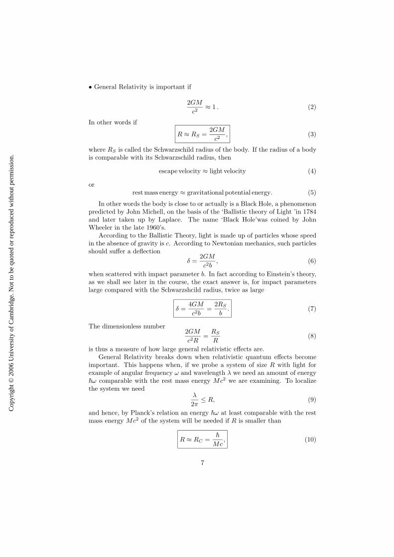
• General Relativity is important if

2GM

c2≈ 1 . (2)

In other words if

R ≈ RS =2GM

c2, (3)

where RS is called the Schwarzschild radius of the body. If the radius of a bodyis comparable with its Schwarzschild radius, then

escape velocity ≈ light velocity (4)

orrestmass energy ≈ gravitational potential energy. (5)

In other words the body is close to or actually is a Black Hole, a phenomenonpredicted by John Michell, on the basis of the ‘Ballistic theory of Light ’in 1784and later taken up by Laplace. The name ‘Black Hole’was coined by JohnWheeler in the late 1960’s.

According to the Ballistic Theory, light is made up of particles whose speedin the absence of gravity is c. According to Newtonian mechanics, such particlesshould suffer a deflection

δ =2GM

c2b, (6)

when scattered with impact parameter b. In fact according to Einstein’s theory,as we shall see later in the course, the exact answer is, for impact parameterslarge compared with the Schwarzshcild radius, twice as large

δ =4GM

c2b=

2RS

b. (7)

The dimensionless number2GM

c2R=

RS

R(8)

is thus a measure of how large general relativistic effects are.General Relativity breaks down when relativistic quantum effects become

important. This happens when, if we probe a system of size R with light forexample of angular frequency ω and wavelength λ we need an amount of energy~ω comparable with the rest mass energy Mc2 we are examining. To localizethe system we need

λ

2π≤ R, (9)

and hence, by Planck’s relation an energy ~ω at least comparable with the restmass energy Mc2 of the system will be needed if R is smaller than

R ≈ RC =~

Mc, (10)

7

Cop

yrig

ht ©

200

6 U

nive

rsity

of C

ambr

idge

. Not

to b

e qu

oted

or

repr

oduc

ed w

ithou

t per

mis

sion

.

where RC is called the Compton radius. If we try to localize a particle to betterthan R ≈ Rc we need so much energy that we run the risk of creating moreparticles. At this point we have to use quantum field theory which is designedto describe systems with an indefinite number of particles because our body willbehave more like an ‘elementary particle ’than a macroscopic body. Thus therealm of classical Newtonian gravity is bounded by R > RS and non-relativisticquantum mechanics by R > RC . These two realms intersect at the Planck scalewhich is the domain of Quantum Gravity. Since very little is known about whathappens there we shall say no more about it in this course except to point outthat associated with it are an absolute or fundamental system of physical units ofmass length and time, independent of any man-made conventions, called Planckunits, characterizing the relevant scale. They work out to be

PlanckMass MP =(c~

G

)12 ≈ 2 × 10−5g ≈ 1019GeV (11)

PlanckLength LP =(G~

c3

)12 ≈ 1.6 × 10−33cm (12)

PlanckTime TP =(G~

c5

)12 ≈ 4 × 10−44s. (13)

2.1 Example

Long before Planck, Johnstone Stoney, the first person to recognize that natureadmits a fundamental unit of electric charge and the man who invented thename ‘electron’constructed an absolute or fundamental system of units using G,and c but not using ~. How did he do it? How are his units related to Planckunits?

3 Review of Newtonian Theory

It will prove useful to review Newtonian theory in a form which we can makecontact with in later work. A freely falling particle has the equation of motion,in an inertial coordinate system, 1

mi

d2x

dt2= mpg(x, t), (14)

where g is the “gravitational field, mi the inertial mass and mp the passivegravitational mass. According to experiments of Galileo, Newton and Eotvoswe have Equality of Inertial and Passive Gravitational Mass, i.e.

mi = mp (15)

and thusd2x

dt2= g(x, t), (16)

1sometimes called an inertial reference frame.

8

Cop

yrig

ht ©

200

6 U

nive

rsity

of C

ambr

idge

. Not

to b

e qu

oted

or

repr

oduc

ed w

ithou

t per

mis

sion

.

which implies the Universality of Free Fall, i.e. all particles fall with the sameacceleration in an external gravitational field. This allows us to pass to a new(non-inertial) coordinate system

x = x + b(t), (17)

in whichd2x

dt2= g(x, t) = g(x, t) − b(t). (18)

We observe that ( cf. Einstein’s Lift)

i) By choosing (t) suitably we can set g = 0 along the path of a single particle.Thus a uniform gravitational field (i.e. one for which g(x, t) is independent x)is unobservable: it can always be eliminated by passing to a suitable frame.

ii) The gravitational field g (i.e. the local value of the acceleration due togravity) is not a physical variable because Newton’s equations of motion admita larger symmetry group (in fact infinite dimensional) than just the Galileigroup.

Following Dicke’s refinement of Einstein’s original analysis it is customaryto describe this situation in terms of the

Weak Equivalence Principle: All freely falling bodies with negligible gravita-tional self interactions follow the same path, if they have the same initial veloc-ity.

This idea is very old, and goes back at least to John Philoponus, a passionatecritic of Aristotle, and who wrote around 500 A.D.

For if you take two weights differing from each other by a very widemeasure, and drop them from the same height, you will see that theratio of the times of their motion does not correspond with the ratioof their weights, but the difference between the times is much less.Thus if the weights did not differ by a wide measure, but if one were,say double, and the other half, the times will not differ at all fromeach other, or if they do, it will be by an imperceptible amount,although the weights did not have that kind of difference betweenthem, but differed in the ratio two to one.

Galileo checked this by timing a ball rolling down an inclined plane and, byrepute, dropping balls from the Leaning Tower of Pisa. Newton made a morequalitative check by showing that the periods of two simple pendula whosebobs are made from different materials are equal to better than one part ina million. Baron Eotvos showed the sun does not exert a periodic torque onthe arm of a torsion balance from which are suspended two weights of differentmaterials. Experiments by Dicke and others have used this method to test theweak equivalence principle by showing that everything on earth falls towards thesun with the same acceleration with a precision of one part in a million million(1012). There are currently plans by NASA and ESA to fly a drag-free satellite

9

Cop

yrig

ht ©

200

6 U

nive

rsity

of C

ambr

idge

. Not

to b

e qu

oted

or

repr

oduc

ed w

ithou

t per

mis

sion

.

(one satellite inside a larger evacuated satellite which has sensors and rocketsto ensure that the inner satellite is in free fall.) using this the proposers planto check Philoponus’ claim to one part in 1017. If his claim fails at this level, apossible explanation would be that in addition to the four forces we are familiarwith (electro-magnetic, weak nuclear, strong nuclear and gravitational) theremay be an additional and so far purely hypothetical long range field responsiblefor a fifth force. Since there is no evidence for such a force we shall, in thiscourse, assume the unrestricted validity of the weak equivalence principle.

By contrast non-uniform gravitational fields are observable. To see how, lookat the motion of two neighbouring particles with positions x and x = x + N.

d2x

dt2= g(x, t), (19)

d2x

dt2= g(x + N) (20)

and sod2N

dt2= (N.grad)g + (O)(N2) (21)

or to the lowest orderd2Ni

dt2= (∂jgi)Nj . (22)

We write this as

d2Ni

dt2+ EijNj = 0. Geodesic Deviation (23)

Eij = −∂jgi. Tidal Tensor (24)

Now the gravitational field is conservative, curlg = 0, and so we may introducethe Newtonian Potential by

g = −gradU gi = −∂iU (25)

whence the tidal tensor is seen to be the Hessian of the Newtonian potential

Eij = ∂i∂jU = Eij . (26)

Now Poisson’s equation or Gauss’s Law relates the gravitational field to thelocal density of active gravitational mass matter ρa:

divg = −4πGρa, (27)

thus∇2U = 4πGρa.2 (28)

2You should check that you understand the signs in (27) and (28) and how and why theydiffer from those in the analogous equations in electro-statics.

10

Cop

yrig

ht ©

200

6 U

nive

rsity

of C

ambr

idge

. Not

to b

e qu

oted

or

repr

oduc

ed w

ithou

t per

mis

sion

.

Now experiment reveals the remarkable fact that the gravitational field gen-erated by a body depends only on its total inertial mass which in turn equals, aswe have seen, its passive gravitational mass. This fact is sometimes known as theprincipal of Identity of Active and Passive Gravitational Mass, or sometimes theStrong Equivalence Principle, since it implies that the Weak Equivalence Prin-ciple will hold even for bodies with significant gravitational self-interactions. InNewtonian theory this follows from Newton’s Third Law that action and reac-tion should be equal and opposite The force F(21) exerted by body 1 on body 2is

F(21) = Gm(2)p m(1)

a

r(1) − r(2)

|r(1) − r(2)|3, (29)

where m(2)p is the passive gravitational mass of body 2 and m

(1)a is the active

gravitational mass of body 2. Now Newton’s Third Law, F(21) = −F(12) requires

m(1)a

m(1)p

=m

(2)a

m(2)p

. (30)

If we require that this equation is true for all possible pairs of bodies, we seethat, by choosing out units sensibly, that active and passive masses must beequal.

In Newtonian theory it then follows that the law of conservation of momen-tum, angular momentum and of the existence of a potential function such thatenergy is conserved will all hold. To some extent the converse holds, if the ThirdLaw did not hold these conservation laws would not necessarily hold.

One simple way to check the Strong Equivalence Principle is by looking atthe motion of the moon. The last astronauts to visit left behind some cornerreflectors, i.e. three plane mirrors meeting mutually at right angles. A laserpulse sent from earth to the moon and into one of these corners is reflected backin precisely the opposite direction3 and by timing how long the pulse takes toget back the orbit the earth moon distance is known to better than a centimetreor so. If the Strong Equivalence principle did not hold one would expect thecentre of mass of the earth moon system to oscillate with the lunar period. Nosuch effect is seen.

Given the identity of inertial, active gravitational and passive gravitationalmass we can drop the subscript and write Poissons’s equation as

Eii = 4πGρ Field Equation. (31)

Finally, because Eij = −∂jgi we have ∂kEij = ∂iEkj or

Ei[j,k] = 0. (32)

One should look upon (32) as an integrability condition for the existence of thegravitational field vector gi. Similarly one should regard the symmetry condition

3You should be able to prove this

11

Cop

yrig

ht ©

200

6 U

nive

rsity

of C

ambr

idge

. Not

to b

e qu

oted

or

repr

oduc

ed w

ithou

t per

mis

sion

.

(26) as an integrability condition for the existence of a Newtonian potential U .Such integrability conditions are often called Bianchi Identities.

We are now in a position to summarize the basic equations and structure ofNewtonian Gravity

1)d2Ni

dt2+ EijNj = 0 Geodesic Deviation

2) Eij = Eji Bianchi Identity

3) Ej[i,k] = 0 Bianchi Identity

4) Eii = 4πGρ Field Equation.

One has that 3) ⇒ Ejk = −∂gj , 3) and 4) ⇒ gi = −∂iU ⇒ Eij = ∂i∂jU

and 4) ⇒ ∇2U = 4πGρ.

3.1 Example

Calculate the tidal tensor due to a spherically symmetric star. The sun andthe moon subtend approximately the same angle (about half a degree) in thesky. They also raise approximately the same tide on earth. Given that tidesare produced by gravity gradients, what can you say about the mean densitiesof the moon and the sun?

4 Review of Special Relativity

I will usually adopt xa = (xi, x4), i = 1, 2, 3, a = 1, 2, 3, 4 as inertial spacetimecoordinates, but sometimes I will call x4 x0 and make the attendent changes ofconventions without further comment. Note that from now indices on coordi-nates will always be “upstairs”. The interval between neighbouring spacetimepoints is

ds2 = dx2 − dt2 = ηabdxadxb, (33)

with ηab = diag(1, 1, 1,−1). In other words we use the “mainly plus” signatureconvention. The interval is invariant under Lorentz transformations

xa → xa = Λabx

b, (34)

whereηabΛ

acΛ

bd = ηcd (35)

or in matrix notationΛtηΛ = η, (36)

where t denotes matrix transpose. The index positions on the matrices maylook unfamiliar, but are consistent with the usual conventions. The first, upper,index labels rows and the second lower index labels columns, and they should bethought of as acting on column vectors xa, where the index labels rows. Strictlyspeaking, Λ is an endomorphism while η is a quadratic form, and for that reason,

12

Cop

yrig

ht ©

200

6 U

nive

rsity

of C

ambr

idge

. Not

to b

e qu

oted

or

repr

oduc

ed w

ithou

t per

mis

sion

.

both of its indices are lowered. For this reason it makes basis independent senseto say that it is symmetric, ηab = ηba.

The Clock Postulate states that a clock moving along a world line xa = xa(λ)with λ some parameter along the curve measures elapsed proper time

τ =

∫

√

−ηabxaxbdλ. (37)

Note that τ is independent of the choice of parameter because if we replace

λ by λ = f(λ) , dxa

dλ= f ′ dxa

dλ, with f ′ = dλ

dλbut

√

−ηab

dxa

dλ

dxb

dλdλ =

√

−ηab

dxa

dλ

dxb

dλdλ (38)

We say that τ is reparametrization invariant.

The Geodesic Postulate states that free particles move on straight lines

d2xa

dλ2= 0 ⇔ xa = xa(0) + λua, (39)

where ua is a constant vector. If the world line is timelike we can normalize ua

by choosing λ to be proper time

λ = τ ⇒ dxa

dλ

dxb

dληab = ηabu

aub = −1. (40)

For light rays this cannot be done and λ is arbitrary up to an affine transforma-tion

λ → aλ + b a, b ∈ R. (41)

We call λ an affine parameter.Free motion can be described using a Variational Principle in at least two

ways:

Method I works only for timelike (or spacelike) curves. We vary the actionfunctional

S[xa(λ)] = −m

∫

√

−ηab

dxa

dλ

dxb

λdλ = −mτ = −m

∫

√

−ηabxaxbdλ. (42)

Note that

i) the action functional S is reparametrization invariant,

ii) Choosing λ = t = x4, we get

S = −m

∫

dt

√

1 −(dx

dt

)2(43)

13

Cop

yrig

ht ©

200

6 U

nive

rsity

of C

ambr

idge

. Not

to b

e qu

oted

or

repr

oduc

ed w

ithou

t per

mis

sion

.

which coincides at small velocities, up to an irrelevant additive piece 4, tothe standard non-relativistic expression. We use the associated Euler-Lagrangeequations

d

dλ

( ∂L

∂xa

)

=∂L

∂xa(44)

with L = −√

−ηabxaxb ⇒ ∂L∂xa = 0. Now

∂L

∂xa= − 1

Lηab

dxb

dλ= −ηab

dxb

dτ(45)

The equation of motion becomes

d

dλ

(

ηab

dxb

dτ

)

= 0 ⇒ d2xa

dτ2= 0. (46)

Method II is rather quicker. We take as action functional

S =

∫

ηab

dxa

dλ

dxb

dλdλ, (47)

L = ηabdxa

dλdxb

dλ. Note that this action is not reparametrization invariant. The

Euler-Lagrange equations are

d

dλ

(

ηab

dxb

dλ

)

= 0. (48)

Now∂L

∂λ= 0, (49)

and so by Noether’s theorem 5

ηab

dxa

dλ

dxb

dλ= constant. (50)

If the constant is negative we choose it to be −1 and find that we can choosethe additive constant in τ so that λ = τ . In this way we recover our previousresult for timelike curves. If the constant is zero, we obtain equations which arevalid for light rays or other massless particles.

It turns out that both Method I and Method II can readily be extended tocurved spacetimes. In practice, Method II is usually more convenient.

It may seem strange that there is no unique action principle for the motionof a particle, but this becomes less so if one reflects that from an abstract point

4You should be able to explain why it is irrelevant.5Check this. You should also check that you understand that there are two cases of

Noether’s theorem, one when the Lagrangian does not depend on the independent variablewhich we are using here and the other when the Lagrangian does not depend upon a dependentvariable, which we will be using shortly. For clarity they should perhaps be called Noether’sfirst and second theorem respectively, but this terminology is not universal.

14

Cop

yrig

ht ©

200

6 U

nive

rsity

of C

ambr

idge

. Not

to b

e qu

oted

or

repr

oduc

ed w

ithou

t per

mis

sion

.

of view we are characterizing the motion as stationary point of a functional, i.eof a function of infinitely many variables. We are familiar with the fact that,in finite dimensions, a given point may be a stationary point of many differentfunctions. To rub home the point you may like to verify that we get the sameequations of motion if we take

L = f(ηab

dxa

dλ

dxb

dλ), (51)

where f() is almost any function of its argument.

5 Curved Spacetime

Because of theUniversality of Free Fall the motion is independent of mass, andso it is an attractive idea to ascribe the curvature of the paths of freely fallingparticles to the curvature of spacetime. We assume that the constant spacetimemetric ηab is replaced by a general space and time dependent curved metricgab(x) such that the interval is given by

ds2 = gab(x)dxadxb, gab = gba. (52)

The Clock and Geodesic Postulates now read as before but with ηab replaced bygab. Thus

τ =

∫

√

−gabxaxbdλ. (53)

Using Method I we have set L =√

−gabxaxb, and the Euler Lagrange equa-tions are

− d

dλ

( 1

L

gabdxb

dλ

)

= − 1

2L

(∂gcd

∂xa

)dxc

dλ

dxd

dλ, (54)

or, since L = 1 if λ = τ ,

d

dτ

(gabdxb

dτ

)

=1

2

(∂gcd

∂xa

)dxc

dτ

dxd

dτ. (55)

This maybe re-written

gab

d2xb

dτ2+

∂gab

∂xc

dxc

dτ

dxb

dτ− 1

2

∂gcd

∂xa

dxc

dτ

dxd

dτ= 0, (56)

or, relabelling dummy indices,

gab

d2xb

dτ2+

1

2

(∂gad

∂xc+

∂gac

∂xd− ∂gcd

∂xa

)dxc

dτ

dxd

dτ= 0. (57)

We define the inverse metric by

gab = (g−1)ab = gba (58)

15

Cop

yrig

ht ©

200

6 U

nive

rsity

of C

ambr

idge

. Not

to b

e qu

oted

or

repr

oduc

ed w

ithou

t per

mis

sion

.

so thatgacgcb = δa

b , (59)

where δab is the Kronecker delta and equal to 1 if a = b and zero otherwise.

Contraction of (57) gea and relabelling e → a now yields

d2xa

dτ2+

ca

d

dxc

dτ

dxd

dτ= 0, (60)

with

ce

d

= 12gea

(

∂gad

∂xc + ∂gac

∂xd − ∂gcd

∂xa

)

. (61)

The rather strange collection of objects

ca

d

are called Christoffel symbols.

We shall explore their mathematical properties shortly. For the time being, theyshould just be thought of as an array of functions, and in fact, to anticipate whatfollows, they are not the components of a tensor field.

We could have proceeded using Method II. A slightly shorter analogous

calculation using L = gabdxa

dλdxb

dλyields

d2xa

dλ2+

ca

d

dxc

dλ

dxd

dλ= 0. (62)

Again we have ∂L∂λ

= 0 and Noether’s theorem yields

gab

dxa

dλ

dxb

dλ= constant. (63)

For massive particles, the constant is negative and we choose it to be −1 andthus get λ = τ . We now obtain our previous equations. However, as in flatspacetime, Method II also works for massless particles.

In the next section we shall apply the equations we have developed to someexamples.

6 Static and stationary metrics, Pound-RebkaExperiment

A metric is called stationary if it is independent of time. This means that onemay introduce a privileged time coordinate t = x4 such ∂

∂t(gab) = 0. Thus

ds2 = g44(x)dt2 + gij(x)dxidxj + 2g4i(x)dtdxi . (64)

A metric is called static if it is stationary and in addition invariant undertime-reversal, i.e. invariant under an involution T : t → −t. This implies thatg4i = 0 and that the metric may be cast in the form

ds2 = hij(x)dxidxj − e2U(x)dt2. (65)

As we shall see shortly, U(x) plays the role of the Newtonian potential.

16

Cop

yrig

ht ©

200

6 U

nive

rsity

of C

ambr

idge

. Not

to b

e qu

oted

or

repr

oduc

ed w

ithou

t per

mis

sion

.

6.1 The Gravitational Redshift

Suppose n pulses are sent from an emitter at xe to an observer at xo in coordi-nate time ∆t. The emitted frequency will, by the clock postulate, be obatinedusing the proper time, so

νe =n

∆t√

−g44(xe)(66)

and similarly for the observed frequency

νo =n

∆t√

−g44(xo)(67)

and hence the ratio

νe

νo

=

√

g44(x0)

g44(xe)= exp

(

U(x0) − U(xe))

. (68)

Evidently if the emitter is at a lower value of the gravitational potential, U(xe) <

U(xo), the received frequency will be lower than the emitted frequency. This iscalled a gravitational redshift and is quantified in terms of a quantity z givenby 1 + z = νe

νo.

We remark that

i) A heuristic derivation of the gravitational redshift can also be given usingPlanck’s relation E = hν and Einstein’s formula E = mc2. One sets up a cyclicprocess in which a photon is sent from a lower to a higher potential, is absorbed,the absorber slowly lowered to the starting point and the photon is then re-emitted. Since energy can be obtained during the lowering process, because ofthe extra weight due to the energy of the absorbed photon, unless the photonloses precisely the predicted amount of energy climbing up the gravitationalwell, one would be able to construct a perpetual motion machine of the secondkind which is impossible.

ii) The gravitational redshift is universal, the redshift experienced is the same

for all massless particles. Again this could also be proved using the impossibilityof perpetual motion machines along the lines given above.

iii) The gravitational redshift shows that as measured by physical clocks, space-time really is curved. This statement is sometimes referred to as the Schildargument.

iv) The gravitational redshift shows that time (i.e. as mesured by clocks) runsat different rates at different places.

v) It is interesting to analyze the problem using the Ballistic Theory accordingto which energy is also conserved. The speed of the ‘light particles’which haveto climb up the gravitational potential well is reduced. Thus according to theBallistic Theory, light coming from different sources will have different speeds.

17

Cop

yrig

ht ©

200

6 U

nive

rsity

of C

ambr

idge

. Not

to b

e qu

oted

or

repr

oduc

ed w

ithou

t per

mis

sion

.

In fact in 1784 John Michell predicted precisely this would happen and suggestedan experiment with a prism to check it. But his prediction contradicts theobserved fact (which we use when setting up Special Relativity) that the speedof light received here on earth is universal and independent of its source.

6.2 Particle motion in Static Spacetimes

We haveL = e2U t2 − hij x

ixj . (69)

In the timelike case we may choose λ = τ . The x4 equation of motion is

d

dτ

(

e2U dt

dτ

)

= 0. (70)

The xi equation of motion is

d

dτ

(

hij

dxj

dτ

)

+ e2U∂iU( dt

dτ

)2=

1

2(∂ihjk)xj xk. (71)

Thus, comparing with 60

44

i

= ∂iU (72)

4i4

= −hij∂je2U (73)

ji

k

=1

2his

(∂hsk

∂xj+

∂hsj

∂xk− ∂hjk

∂xs

)

. (74)

Independence of t gives, from Noether’s theorem,

e2U dt

dτ= E, (75)

where the constant E is the energy. Now gabxaxb = −1 (with λ = τ) gives

e2U( dt

dτ

)2 − hij

dxi

dτ

dxj

dτ= 1 = E2e−2U − hij

dxi

dτ

dxj

dτ. (76)

6.3 The Newtonian Limit

In the above we have set c = 1. To understand this approximation we shouldrestore units and so t → ct. The quantity U is replaced by U

c2 .Now we can now expand the metric in inverse powers of c:

g44 = −c2 + O(1) (77)

hij = δij + O(1

c2) . (78)

Now

e2U

c2 = 1 +2U

c2+ . . . . (79)

18

Cop

yrig

ht ©

200

6 U

nive

rsity

of C

ambr

idge

. Not

to b

e qu

oted

or

repr

oduc

ed w

ithou

t per

mis

sion

.

Thus, to the lowest non-trivial order, we put

ds2 ≈ −c2dt2(1 +2U

c2) + dx2

(

1 + O(1

c2))

. (80)

If we, in addition, assume that the particle is moving slowly, we may setτ ≈ t, E = 1 + E . We find from (76)

1

2v2 + U = E . (81)

Clearly, this is the equation of energy conservation for a non-relativistic particleof energy per unit mass E moving in a Newtonian gravitational potential U .This justifies our identification of the quantity 1

2 ln(−g44) as the Newtonianpotential.

In fact, using the Einstein field equations, which we have not yet met, it ispossible to improve (80) so that it is accurate to order 1

c4

ds2 ≈ −c2dt2(1 +2U

c2) +

(

1 − 2U

c2

)

dx2. (82)

We can now give the gravitational redshift suffered by a photon in the fieldof a body of mass M in the Newtonian approximation

νo

νe

= GM(1

re

− 1

ro

). (83)

For the Pound-Rebka experiment ro = re +h, where h is the height of the tower,we obtain

δν

ν=

gh

c2. (84)

6.4 Motion of Light rays

Noether’s theorem gives

e2U dt

dλ= E, (85)

and the fact that gabxaxb = 0 gives (cf. 76)

E2 = e2Uhij

dxi

dλ

dxj

dλ, (86)

d2xi

dλ2+

[

ji

k

+ hjkhis∂sU]dxj

dλ

dxk

dλ= 0. (87)

Because the affine parameter λ is defined only up to an overall multiple,λ → aλ, so too is the ‘Energy’E. The equations are invariant under the rescalingλ → aλ, E → E

a. This means that, in a purely particle theory of light, only the

ratio of energies is well defined.The interpretation of (87) will be given later in the course.

19

Cop

yrig

ht ©

200

6 U

nive

rsity

of C

ambr

idge

. Not

to b

e qu

oted

or

repr

oduc

ed w

ithou

t per

mis

sion

.

6.5 Further Examples

6.5.1 The Schwarzschild Metric

You should now be in a good position to study the motion of particles movingaround a spherically symmetric static black hole or a star. Provided the orbitingparticle has a negligible effect on the spacetime geometry, which will be true ifit is very much less massive than the star or black hole, the metric is

ds2 =dr2

1 − 2Mr

+ r2(dθ2 + sin2 θdφ2) −(

1 − 2M

r

)

dt2. (88)

We will take a more detailed look at this later in the course.

6.5.2 The k = 0 Robertson-Walker Metric

Our universe is not static, but rather it is expanding. To a good approximationthe metric of our universe is given by 6

ds2 = −dt2 + a2(t)dx2. (89)

The function a(t) is called the scale factor. For a particle of mass m,Noether’s theorem implies momentum conservation

ma2(t)dx

dλ= p, (90)

where p is a constant vector, but because of the time-dependence, energy

E = mdt

dτ(91)

is not conserved. In fact using the normalization of the 4-velocity one gets

E =

√

m2 +p2

a2(t). (92)

Thus if the universe expands and the scale factor a(t) increases the energy E

decreases. The locally measured (so-called ‘peculiar’) velocity

v = a(t)dx

dt(93)

given by

v =p

√

p2 + m2a2(t)(94)

also decreases except in the limit of zero mass m when v is constant and of unitmagnitude |v| = 1. The energy of a massless particle decreases ∝ 1

a(t) , thus if a

photon is emitted at time te and received at time to the redshift is given by

E(te)

E(te)= 1 + z =

a(to)

a(te). (95)

6In cosmology one studies a more general class of Robertson-Walker metrics in which thespatial sections are curved.

20

Cop

yrig

ht ©

200

6 U

nive

rsity

of C

ambr

idge

. Not

to b

e qu

oted

or

repr

oduc

ed w

ithou

t per

mis

sion

.

6.5.3 Example: End point variations and momentum conservation

If the end points of the world line from A to X are allowed to vary, the variationof the action S(X,A) is

δS(X,A) =

∫ X

A

δxa( ∂L

∂xa− dpa

dλ

)

dλ +[

paδxa]X

A, (96)

where the canonical momentum pa is defined by

pa =∂L

∂xa. (97)

Now consider a 2-particle collison at X in which particle 1 with mass m1 startsfrom A, particle two with mass m2 from B and after the collision particle 3arrrives at C with mass m3 and particle 4 arrives at D with mass m4. We varythe total action and demand that it vanish:

δS(C,X) + δS(D,X) + δS(X,A) + δS(X,B) = 0, (98)

where the points A,B,C,D are held fixed but X is allowed to vary. As well aslearning that AX, BX, XC and XD must be geodesics, we also discover fromthe variation at X that momentum is conserved at the collision:

p1a + p2

a = p3a + p4

a, (99)

where

pia = migab

dxb

dτ. (100)

7 Lengths, Angles and Conformal Rescalings

An important aspect of General Relativity is that locally the laws of SpecialRelativity should hold. Thus if we work in a small neigbourhood of a point xa

in spacetime, we can use the metric gab to define an inner product

gabVaU b (101)

on infinitesimal vector displacements V a, Ua and define the length of a vectorV a by

|V a| =√

|gabV aV b|. (102)

If the two vectors are spacelike, the angle θ between them is given by

cos θ =gabU

aV b

|Ua||V b| . (103)

If the two vectors are timelike, and both are future directed, the rapidity θ

between them is given by

cosh θ = −gabUaV b

|Ua||V b| . (104)

21

Cop

yrig

ht ©

200

6 U

nive

rsity

of C

ambr

idge

. Not

to b

e qu

oted

or

repr

oduc

ed w

ithou

t per

mis

sion

.

If we change the metric by multiplying by a positive function (a processcalled Weyl-rescaling):

gab → Ω2(x)gab = gab (105)

we find that all lengths rescale

|V a| → Ω|V a|, (106)

but angles and rapidities are unchanged

θ → θ. (107)

For this reason Weyl-rescalings are also called Conformal Rescalings. An im-portant example is provided by the time-dependent Robertson-Walker metricof an expanding universe

ds2 = −dt2 + a2(t)dx2 = a2(t)(

−dη + dx2)

(108)

which is obtained by a conformal rescaling of the flat and static Minkowskimetric inside the bracket. The coordinate η is defined by

η =

∫

dt

a(t), (109)

and Ω(x) = a(t). As we shall see later, the null geodesics of two conformallyrelated metrics coincide. It follows that the angles made by system of lightrays in this type of expanding universe are the same as they would be in flatspacetime.

For example, a galaxy emitting light of intrinsic proper size d at time te hassize d

a(te) in the conformally related Minkowski metric and thus subtends an

angle (assumed very small) at time to given by

∆θ =d

a(te)(ηo − ηe), (110)

where

ηo − ηe =

∫ to

te

dt

a(t). (111)

The formula (110) has an amusing consequence. If we consider a familyof galaxies, all of the same intrinsic size, at greater and greater distances, orequivalently greater and greater redshifts, the apparent angular size at first de-creases, as we should expect in flat spacetime, and then increases. For example,if a(t) ∝ tp, with 0 < p < 1 a short calculation, which you should check, showsthat the apparent angular size is least at a redshift

1 + z =(1

p

)

p

1−p . (112)

22

Cop

yrig

ht ©

200

6 U

nive

rsity

of C

ambr

idge

. Not

to b

e qu

oted

or

repr

oduc

ed w

ithou

t per

mis

sion

.

Which metric is the ‘correct’metric depends upon our measuring instru-ments. If we use conventional measuring instruments, built say of ordinaryatoms, we find that they measure lengths as given by the Roberston-Walkermetric, and relative to them the universe expands. Of course it is always possi-ble to maintain, rather as one imagines Alice would have, that the universe isnot expanding but it is we who are getting smaller, but if she had she wouldhave also have had to agree that the atoms of which she is made are also gettingsmaller. If one really wishes to maintain that the flat Minkowski metric is the‘correct’one, one should provide a set of instruments which measure it.

It is perhaps striking that philosophical speculations about what would hap-pen if the universe doubled in size overnight and whether we would notice werequite frequent towards the end of the nineteenth century, long before Einsteinformulated General Relativity. Only later in the 1920’s with Hubble’s discoveryof the expansion of the universe did they become relevant for physics.

8 Tensor Analysis

One can only get so far using just geodesics. To make further progress and tobe able to write down the analogue of Poisson’s equation, i.e. Einstein’s fieldequations, we need to develop some more geometry. In this introductory coursewe shall proceed at what is mathematically a relatively unsophisticated level.Much deeper accounts of differentiable manifolds can of course be given, butfor practical purposes they are much less relevant than a good understandingof what has become a standard part of Mathematical Physics.

Our analysis of the Weak Equivalence Principle shows that privileged globalinertial coordinates cease to exist in a general curved spacetime. Our formalismmust therefore allow the use of arbitrary coordinate systems. This desire isformalized in the

Principle of General Covariance which states that one should be able to writedown the equations of physics in a way which is valid in all coordinate systems.

Such equations are said to be covariant or sometimes form-invariant since theyshould take the same form in all coordinate systems. It is important to realizethat the Principle of General Covariance does not preclude the use of particularcoordinate systems which may be extremely useful in practice. Neither does itrule out a priori the possibility of privileged systems of coordinates or frames ofreference. It simply requires that such spacetimes can in principle be describedwithout reference to particular cordinate systems. Thus if spacetime really wereflat, we would like to say so without introducing global inertial coordinates.Tensor Calculus or Tensor Analysis allows us to do just that.

Given one coordinate system xa we can always pass to a new coordinatesystem xa = xa(xb) and calculate the Jacobian matrix

Λab =

∂xa

∂xb. (113)

23

Cop

yrig

ht ©

200

6 U

nive

rsity

of C

ambr

idge

. Not

to b

e qu

oted

or

repr

oduc

ed w

ithou

t per

mis

sion

.

The chain rule implies that if ˜xa

= ˜xa(xc) is a third coordinate system, then

∂ ˜xa

∂xb=

∂ ˜xa

∂xc

∂xc

∂xb. (114)

Moreover, if the transformation xa → xa is invertible

det(∂xa

∂xb

)

6= 0, (115)

we have

∂xa

∂xb

∂xb

∂xc= δa

c . (116)

For example, for a linear transformation, such as a Lorentz transformation,

xa = Λabx

b,∂xa

∂xb= Λa

b, (117)

the Jacobian matrix is a constant matrix. Note how nicely the index posi-tions accommodate themselves to the rules of partial differentiation and matrixmultiplication, and of course, the Einstein summation convention.

One sometimes encounters the use of tildes on the indices as a further aid toremembering what variables are being differentiated. In that case, the Einsteinsummation convention holds but repeated indices must be of the same type, i.e.either both un-tilded or both tilded. I shall not adopt that usage here becauseit strains the eye and tends to make printed formulae difficult to read. Howeverfor beginners, or when engaged in complicated calculations, this notation canbe useful.

We now consider Vector Fields. To motivate the definition consider a curvexa = xa(λ) in spacetime. Its tangent vector in the xa coordinates is (by defini-tion)

T a =dxa

dλ, (118)

and in coordinates xa, it is

T a =dxa

dλ. (119)

Using the chain ruledxa

dλ=

∂xa

∂xb

dxb

dλ, (120)

and thus

T a =∂xa

∂xbT b, contravariant vector field. (121)

This formula motivates the definition of what is called a contravariant vectorfield as set of quantities T a(x) transforming under a coordinate change as (121).

24

Cop

yrig

ht ©

200

6 U

nive

rsity

of C

ambr

idge

. Not

to b

e qu

oted

or

repr

oduc

ed w

ithou

t per

mis

sion

.

The strange epithet contravariant suggests that there is some other kind ofvector field. This is true, and they are called covariant vector fields and roughlyspeaking, they transform in the opposite way. An example is the gradient

Fa = ∂af =∂f

∂xa(122)

of a function f(x). The chain rule gives

∂f

∂xa=

∂xb

∂xa

∂f

∂xb, (123)

or, if Fa = ∂f∂xa

,

Fa =∂xa

∂xbFb, covariant vector field (124)

If the coordinate transformation xa → xa is invertible, we also have

Fa =∂xb

∂xaFb, , . (125)

Given a contravariant vector field T a and a covariant vector field Fa, onemay form the contraction FaT a = T aFa. Because

FaT a =∂xa

∂xb

∂xe

∂xaT bFe = δe

bTbFe = T aFa, (126)

the contraction is invariant, that is, it is a scalar field.The transformation properties of the metric tensor field follow, just as in

Special Relativity, by demanding that the interval

ds2 = gabdxadxb = gcddxcdxd (127)

is invariant. Now since,

dxa =∂xa

∂xcdxc, (128)

we have

gcd = gab

∂xa

∂xc

∂xb

∂xd, symmetric second rank covariant tensor field . (129)

A general (not necessarily symmetric) second rank covariant tensor field Qab

transforms as

Qcd = Qab

∂xa

∂xc

∂xb

∂xd, symmetric second rank covariant tensor field . (130)

We can decomposeQcd = Q(cd) + Q[dc], (131)

25

Cop

yrig

ht ©

200

6 U

nive

rsity

of C

ambr

idge

. Not

to b

e qu

oted

or

repr

oduc

ed w

ithou

t per

mis

sion

.

into

Q(cd) =1

2

(

Qcd + Qdc

)

= Q(dc) its symmetric part (132)

and

Q[cd] =1

2

(

Qcd − Qdc

)

= −Q[dc] its anti−symmetric part. (133)

This decomposition is invariant under a general coordinate transformation.Thus, for example

Q(cd)∂xc

∂xa

∂xd

∂xc= Qcd

∂x(c

∂xa

∂xd)

∂xc= Qcd

∂xc

∂x(a

∂xd

∂xb)=

(

Q)

(ab). (134)

An identical argument holds for the anti-symmetric part with round bracketsexchanged for square brackets.

One may define contravariant second rank tensors analogously

P ab = P cd ∂xa

∂xc

∂xb

∂xc. (135)

Again the symmetric and anti-symmetric parts transform into themselves undergeneral coordinate transformations.

In general, one may consider arbitrary tensor fields of type(p

q

)

with

p indices upstairs, i.e. contravariant

q indices downstairs, i.e. covariantThe transformation rule now has p factors of ∂x

∂xand q factors of ∂x

∂x.

For example a(1

1

)

tensor field transforms as

Mab =

∂xa

∂xc

∂xd

∂xbM c

d . (136)

The upstairs and downstairs indices can be contracted to yield a scalar calledthe trace

Maa =

∂xa

∂xc

∂xd

∂xaM c

d = δdc M c

d = Mdd. (137)

In general, one may always contract r contravariant indices with r covariant

indices and the contraction will be a tensor field of type(p−r

q−r

)

, r ≤ min(p, q).

8.1 Operations on tensors preserving their tensorial prop-erties

(i) Addition (of same type)

(ii) Multiplication by scalars

(iii) Outer or Tensor Products, e.g.

VaW b is a(1

1

)

tensor. (138)

26

Cop

yrig

ht ©

200

6 U

nive

rsity

of C

ambr

idge

. Not

to b

e qu

oted

or

repr

oduc

ed w

ithou

t per

mis

sion

.

(iv) Contractions

(v) Index Interchange

Tab is a tensor ⇔ Tba is a tensor. (139)

(vi) Symmetrization and Anti-symmetrization. For example

T[abc] =1

3!

(

Tabc + Tcab + Tbca − Tbac − Tcba − Tacb

)

is a tensor . (140)

8.2 Quotient Theorem

For example, if V abWab is a scalar for an arbitrary contravariant tensor V ab,then Wab is a covariant tensor. This result is sometimes called Tensor Detection.

8.3 Rules for Index Shuffling

For exampleV (ab)Wab = V abW(ab), (141)

andV (ab)W[ab] = 0. (142)

8.4 *Graphical Notation*

For some purposes, especially those involving complicated index manipulations,it may be convenient to adopt a graphical or ‘chemical’notation for tensors firstintroduced by Clifford, Cayley and Sylvester in the nineteenth century. In thisnotation

(i) Each tensor is represented by a vertex,

(ii) A contravariant index is represented by attaching an edge with an outgoingarrow on it

(iii) A covariant index is represented by by an ingoing arrow.

(iv) In order to keep track of the order of the indices the arrows are attached ina definite cyclic order, for example anti-clockwise, around each node. Of coursethe relative order of an ingoing and outgoing node is unimportant

(v) Contractions correspond to joining an ingoing and an outgoing arrow, notnecessarily attached to the same vertex.

(vi) The Kronecker delta δba is represented by a nodeless arrow.

If one has a distinguished metric or bi-linear form, then the arrows may beomitted. The obvious analogy with chemical diagrams explains why a tensorof type

(p

q

)

is sometimes said to have valence p + q. The main draw-back of

this notation is the need to keep track of the cyclic order. Of course for totallysymmetric or totally anti-symmetric tensors, this is not a problem since then

27

Cop

yrig

ht ©

200

6 U

nive

rsity

of C

ambr

idge

. Not

to b

e qu

oted

or

repr

oduc

ed w

ithou

t per

mis

sion

.

lifting one arrow over another of the same type gives rise to the same tensorup to a sign. This can be used to give graphical proofs of tensor identitiesor the enumeration of all possible invariants constructed from a set of tensors.The latter problem is analogous to counting the number of isomers of a certainmolecule.

9 Differentiating Tensors

We have seen that ∂φ∂xa is a co-vector field but what about the Hessian?

∂φ

∂xa∂xb=

∂xc

∂xa

∂

∂xc

(∂xd

∂xb

∂φ

∂xd

)

(143)

=∂xc

∂xa

∂xd

∂xb

∂2φ

∂xc∂xd+

∂xc

∂xa

∂2xd

∂xc∂xb

∂φ

∂xd(144)

=∂xc

∂xa

∂xd

∂xb

∂2φ

∂xc∂xd+

∂2xd

∂xa∂xb

∂φ

xd. (145)

The first term is good but the second is clearly bad. In other words, the Hessianis not a second rank covariant tensor field. For similar reasons, neither are the

Christoffel symbols

ab

c

the components of a tensor field of type(1

2

)

.In order to construct tensor fields we must introduce a so-called covariant

derivative operator ∇a which maps(p

q

)

tensors to(

pq+1

)

tensors . Moreover we

want ∇a to have properties as close as possible to those of ∂a.We demand of ∇a that

(i) ∇aφ = ∂aφ,

(ii) ∇ is Leibnizian:

∇a(UV ) = (∇aU)V + U(∇aV ), (146)

for any pair of(p

q

)

and(p′

q′

)

tensor fields U and V ,

(iii) ∇a commutes with contractions,

(iv) Acting on a vector field,

∇aV b = ∂aV b + Γab

cVc. (147)

A covariant derivative operator is also called an affine connection and theΓa

bc are its components 7.

7For a general affine connection, there is no symmetry with respect to interchange of thethe lower indices. I am using the convention that the first index is the ‘differentiating’index.This convention is not in universal use, and so one should take care when consulting text-books. However, shortly we will restrict attention to symmetric affine connections and thisdistinction becomes unnecessary.

28

Cop

yrig

ht ©

200

6 U

nive

rsity

of C

ambr

idge

. Not

to b

e qu

oted

or

repr

oduc

ed w

ithou

t per

mis

sion

.

They are not the components of a1

2

tensor field. In fact, under a coordi-nate transformation

Γab

c → Γab

c =∂xb

∂xe

∂xg

∂xa

∂xd

∂xcΓg

ed +

∂xb

∂xe

∂2xe

∂xa∂xc. (148)

Properties (i),(ii),(iii),(iv) determine the action of the covariant derivativeoperator ∇a on any tensor field. For example, to see how ∇a acts on a covectorfield note that

∇a(WbVb) = (∇aWb)V

b + Wb(∇aV b) = ∂a(WbVb) (149)

= (∂aWb)Vb + (∂aV b)Wb = (∇aWb)V

b + Wb(∂aV b + Γab

cVc), (150)

which implies that

∇aWb = ∂aWb − Γac

bWc . (151)

Note the minus sign compared with the expression (iv) for a vector field.Similarly,

∇aWcb = ∂aWcb − Γae

cWeb − Γae

bWce . (152)

It is a useful exercise to check that

∇a∇bφ = ∇a∂bφ (153)

are the components of a tensor field.

9.1 Symmetric Affine Connections

Using index shuffling and the equality of mixed partials we deduce that

Γ[ab

c] =∂xb

∂xe

∂xg

∂x[a

∂xd

∂xc]Γg

ed (154)

=∂xb

∂xe

∂x[g

∂xa

∂xd]

∂xcΓg

ed (155)

=∂xb

∂xe

∂xg

∂xa

∂xd

∂xcΓ[g

ed] . (156)

It follows thatTa

bc = Γa

bc − Γc

ba = −Tc

ba (157)

is a tensor of type(1

2

)

called the torsion tensor. In what follows, we shallalways assume that the torsion vanishes, i.e the components of the connectionare symmetric

Γab

c = Γcb

a . (158)

You should check that you understand why the work we did above shows thatthis is a statement which holds in all coordinate systems.

29

Cop

yrig

ht ©

200

6 U

nive

rsity

of C

ambr

idge

. Not

to b

e qu

oted

or

repr

oduc

ed w

ithou

t per

mis

sion

.

9.1.1 Example: Exterior Derivative

An anti-symmetric co-tensor is called a p-form.One may construct a (p+1) form, called the exterior derivative or generalized

curl, using just partial differentiation. We define 8

dωabc... = (p + 1)∂[aωbc...]. (159)

To prove this is a tensor field we can either write out the behaviour under a coor-dinate transformation and see that the bad terms cancel, or more expeditiously,show that for any symmetric affine connection

∂[aωbc...] = ∇[aωbc...]. (160)

The right hand side is a tensor and therefore the left hand side is a tensor. Theoperator d so defined acting on p forms is nilpotent: d2 = 0.

9.1.2 Example: The Nijenhuis Bracket

Similarly, using the same technique, one may prove that given two(1

1

)

tensorfields Aa

b and Bab, then

Sab

c = Aea∂eB

bc−Ab

e∂aBec−Ae

c∂eBb

a+Abe∂cB

ea+Be

a∂eAb

c−Bbe∂aAe

c−Bec∂eA

ba+Bb

e∂cAe

a

(161)

is also a(1

2

)

tensor field which is antisymmetric in a and c.

9.2 The Levi-Civita Connection

It is a striking fact that

(i)

ba

c

=

ca

b

(162)

(ii)

ba

c

transform precisely as a symmetric affine connection.We call this connection the Levi-Civita connection. It has the following

remarkable property

∇agbc = ∂agbc − Γae

bgec − Γae

cgeb = 0. (163)

In fact, a stronger statement is true

The Fundamental Theorem of Differential GeometryThe Levi-Civita connection

ba

c

is the unique affine connection s.t.

(i)Γb

ac = Γc

ab, i.e. is symmetric (164)

8The p+1 factor is conventional and makes for simplifications in the formulation of Stokes’stheorem.

30

Cop

yrig

ht ©

200

6 U

nive

rsity

of C

ambr

idge

. Not

to b

e qu

oted

or

repr

oduc

ed w

ithou

t per

mis

sion

.

(ii)∇agcb = 0, themetric is covariantly constant. (165)

Proof: We write out the covariant constancy condition three times, cyclicallypermuting the three indices and then take a suitable linear combination. Thesymmetry of Γa

bc leads to cancellations:

(i) ∇agbc = ∂agbc − Γae

bgec − Γae

cgeb = 0. (166)

(ii) ∇cgab = ∂cgab − Γce

ageb − Γce

bgea = 0. (167)

(iii) ∇bgca = ∂bgca − Γbe

cgea − Γbe

agec = 0. (168)

Now take (i) − (ii) − (iii) and use the symmetry of the connection to get

2geaΓbe

c + ∂agbc − ∂cgab − ∂bgac = 0, (169)

which gives

Γbe

c =1

2ges

(

∂bgsc + ∂cgsb − ∂sgbc

)

. (170)

9.2.1 Example: metric-preserving connections with torsion

Repeat the above exercise for a connection with torsion to find that the connec-tion coefficients are now given by

Γbe

c =1

2ges

(

∂bgsc + ∂cgsb − ∂sgbc

)

+ Tbe

c − Tbce − Tcb

e. (171)

The additional term

Kbe

c = Tbe

c − Tbce − Tcb

e (172)

is sometimes called the contorsion tensor.

10 Parallel transport

If γ is a curve given by xa(λ) and T a = dxa

dλits tangent vector we define the

absolute derivative of a vector V a along γ by

DV a

Dλ= T b∇bV

a . (173)

We often denote ∇bVa by V a

;b and so

DV a

Dλ= V a

;bTb. (174)

31

Cop

yrig

ht ©

200

6 U

nive

rsity

of C

ambr

idge

. Not

to b

e qu

oted

or

repr

oduc

ed w

ithou

t per

mis

sion

.

We say that V a is parallely transported along γ if

DV a

Dλ= 0. (175)

That isdV a

dλ+ (T bΓb

ac)V

c = 0, (176)

or, infinitesimally,dV a = −Γb

aeV

edxb (177)

along γ. This is a linear o.d.e. along γ and has a unique solution given theinitial value of the vector, V a(0). However parallel transport is path dependent,it depends on γ and two curves γ and γ′ joining the same two events in spacetimewill have different vectors V a at the end points.

Note that we could have demanded the apparently weaker condition

DV a

Dλ= f(λ)V a (178)

along γ for some function f(λ), but if

V a = gUa, (179)

we have

gUa + gDUa

Dλ= fgUa, (180)

and so, by setting gg

= f , we get

DUa

Dλ= 0. (181)

10.1 Autoparallel curves

These are curves along which the tangent vector T a is parallely transported 9

DT a

Dλ= 0 (182)

or

d2xa

dλ2+ Γb

ac

dxc

dλ

dxb

dλ= 0 . (183)

For the Levi-Civita connection, Γab

c =

ab

c

we recover our old definitionof a geodesic.

9Although we won’t use this fact in this course, the notions of parallel transport and auto-parallel curve also make sense for affine connections which are not necessarily symmetric.

32

Cop

yrig

ht ©

200

6 U

nive

rsity

of C

ambr

idge

. Not

to b

e qu

oted

or

repr

oduc

ed w

ithou

t per

mis

sion

.

Note that we could have demanded the apparently weaker condition that

DT a

Dλ= f(λ)T a, (184)

for some f(λ). However if we change parameter

λ → λ = λ(λ), (185)

we findT a = gT a, (186)

where

g =dλ

dλ, T a =

dxa

dλ, (187)

and we can now use our previous remark to set gg

= f and find a new parameter

λ such thatDT a

Dλ= 0, (188)

and we get back to our previous condition. Such a choice of parameter is calledan affine parameter and it is unique up to an affine transformation

λ → aλ + b, a, b ∈ R. (189)

10.2 Acceleration and Force

Let τ be proper time along a timelike curve γ, then the 4-acceleration is definedby

aa =DUa

Dτ, (190)

where Ua = dxa

dτis the 4-velocity and is normalized so that UaUa = gabU

aU b =−1.

Differentiating gabUaUb = 1 along γ and remembering that the metric is

covariantly constant, Dgab

Dλ= 0, we find that

2Uaaa = 0. (191)

Thus the 4-velocity and acceleration vector are orthogonal, in particular theacceleration vector is spacelike. The 4-force F a is defined by

d(mUa)

dτ= F a, (192)

where m is the rest mass of the particle, which we will assume is a constant.In this case Newton’s law holds in the form F a = maa. Any expression for theforce must be orthogonal to the 4-velocity

F agabUb = 0. (193)

33

Cop

yrig

ht ©

200

6 U

nive

rsity

of C

ambr

idge

. Not

to b

e qu

oted

or

repr

oduc

ed w

ithou

t per

mis

sion

.

10.2.1 Example: The acceleration of a particle at rest

A particle at rest in a static metric has Ua = 1√|g44|

δa4 and a 4-acceleration

Ua = −(∂ig44

2g44, 0). (194)

Thus the 4-acceleration a particle at rest is directed radially outward and itsmagnitude squared is given by

UaUa =1

4(g44)2hij∂ig44∂jg44. (195)

In the Schwarzschild metric, this equalsM2

r4

1− 2Mr

. The acceleration, and hence the

force needed to keep the particle from falling radially inwards, diverge at thehorizon r = 2M .

To check that this is reasonable, it is worth working through this examplein the case of 2-dimensional Minkowski space E 1,1 in accelerating coordinateswhich is a good local model for the behaviour of the metric near a Killing horizonas we shall see later. If

x0 = ρ sinh t, x1 = ρ cosh t, (196)

the metric in the Rindler wedge x1 > |x0| is

ds2 = −ρ2dt2 + dρ2. (197)

Curves ρ = constant have acceleration 1ρ

and this is clearly in the positive

x1 direction.

10.2.2 Example: Charged Particles

For a particle of charge e moving in an electromagnetic field we have the Lorentzequation

mDUa

Dλ= eF a

bUb, (198)

whereFab = gacF

cb = −Fba = F[ab], (199)

is the second rank antisymmetric covariant Faraday tensor, the Lorentz 4-forceis indeed orthogonal to the 4-velocity.

10.2.3 Example: Relativistic Rockets

Relativistic rockets have variable rest-mass, m = m(τ). Their equation of mo-tion is

DmUa

Dτ= Ja, (200)

34

Cop

yrig

ht ©

200

6 U

nive

rsity

of C

ambr

idge

. Not

to b

e qu

oted

or

repr

oduc

ed w

ithou

t per

mis

sion

.

where Ja is the rate of emission of 4-momentum of the ejecta. Physically Ja

must be timelike, JaJa < 0, which leads to the inequality

m

m> |aa|. (201)

Thus to obtain a certain acceleration, as in the Twin-Paradox set-up, over acertain proper time requires a lower bound on the total mass of the fuel used

ln(mfinal

minitial) <

∫

|aa|dτ. (202)

In two dimensional Minkowski spacetime E 1,1

Ua = (cosh θ, sinh θ) ⇒ |aa| =dθ

dτ, (203)

where θ is the rapidity. We find

mfinal

minitial<

√

1 + vinitial

1 − vinitial

√

1 − vfinal

1 + vfinal=

1

1 + z. (204)

Consider two observers, one of whom is at rest and engaged in checkingGoldbach’s conjecture that every even number is the sum of two primes using acomputer. The second observer, initially at rest with respect to the first observervinitial = 0, decides to use time dilation to find out faster by accelerating towards

the stationary observer thus acquiring a velocity vfinal and a blue shift factor(1+z). The increase in the rate of gain of information is bounded by the energyor mass of the fuel expended.

10.3 The Levi-Civita connections of conformally relatedmetrics

Supose we have two conformally related metrics such that

g′ab = Ω2gab. (205)

A short calculation reveals that

ba

c

′=

ba

c

+ δab

∂cΩ

Ω+ δa

c

∂bΩ

Ω− gas ∂sΩ

Ωgbc (206)

Now, given a curve γ, xa(λ) we have

d2xa

dλ2+

ba

c

′ dxb

dλ

dxc

dλ=

d2xa

dλ2+

ba

c

dxb

dλ

dxc

dλ+2

dxa

dλ

Ω

Ω−gas ∂sΩ

Ωgab

dxa

dλ

dxb

dλ.

(207)Now, in general, if xa(λ) is a geodesic of the metric gab it will not be a

geodesic of the metric g′ab. However there is an exception. Supposing that γ isa null geodesic of the metric gab then we have

gab

dxa

dλ

dxb

dλ= 0 ⇒ g′ab

dxa

dλ

dxb

dλ= 0, (208)

35

Cop

yrig

ht ©

200

6 U

nive

rsity

of C

ambr

idge

. Not

to b

e qu

oted

or

repr

oduc

ed w

ithou

t per

mis

sion

.

and so γ certainly has a null tangent vector with respect to the confomallyrelated metric g′ab. Now

d2xa

dλ2+

ba

c

′ dxb

dλ

dxc

dλ=

d2xa

dλ2+

ba

c

dxb

dλ

dxc

dλ+ 2

dxa

dλ

Ω

Ω, (209)

and so if xa(λ) is a null geodesic of the metric gab with λ an affine parameter,then the left hand side vanishes and we deduce from the vanishing of the righthand side that it is also a null geodesic of the conformally related metric g′ab.But now λ is no longer an affine parameter. Thus while being a null geodesic isa conformally invariant statement, being affinely parametrized is not.

Physically two conformally related metrics cannot be distinguished by meansof measurements made solely with light rays.

10.4 Static metrics and Fermat’s Principle

If

ds2 = −e2Udt2 + hijdxidxj (210)

we found that the equation of motion of a photon is

d2xi

dλ2+

[

ji

k

+ hishjk∂sU]dxj

dλ

dxk

dλ= 0 . (211)

Now introduce a new spatial metric

h′ij = e−2Uhij . (212)

One has

ji

k

′=

ji

k

− δij∂kU − δi

k∂jU + his∂sUhjk. (213)

Thusd2xi

dλ2+

ji

k

′ dxj

dλ

dxk

dλ= 2

dxi

dλ∂kU

dxk

dλ. (214)

It follows that xλ is a non-affinely parmetrized geodesic of the optical or Fermat3-metric

ds2o = e−2Uhijdxidxj = h′

ijdxidxj . (215)

Sinceds2

4 = e2U[

− dt2 + h′ijdxidxj

]

, (216)

this is, in fact, a special case of our previous example with Ω = eU .

36

Cop

yrig

ht ©

200

6 U

nive

rsity

of C

ambr

idge

. Not

to b

e qu

oted

or

repr

oduc

ed w

ithou

t per

mis

sion

.

10.4.1 Isotropic coordinates and optical metric for the Schwarzschildsolution: Shapiro time delay

Any spherically symmetric 3-metric is conformally flat10. In fact, if one intro-duces an isotropic coordinate ρ by

r = ρ

(

1 +M

2ρ

)2

, (217)

which maps ∞ > ρ > M2 to ∞ > r > 2M in a 1-1 way, then the Schwarzschild

metric becomes

ds2 = −(1 − M

2ρ

1 + M2ρ

)2

dt2 +(

1 +M

2ρ

)4

dρ2 + ρ2(

dθ2 + sin2 θdφ2)

(218)

The 3-metric inside the brace is flat. Thus the optical metric is of the form

ds2o = n2(x)dx2, (219)

and n(x) is an effective space-dependent refractive index given by

n(x) =

(

1 + M2|x|

)3

(

1 − M2|x|

) . (220)

The effective refractive index n(x) increases from unity at infinity to infinity asone approaches the horizon at r = 2M,ρ = M

2 . Light or radio waves passingnear a star or black hole are thus slowed down compared with radio waves orlight which keep away. This effect is called the Shapiro time delay effect and hasbeen verifed recently (using the Cassini satellite when it was in opposition to theearth) to one part in a hundred thousand 11. A radio wave is sent from earth tothe satellite and back. To the relevant accuracy, the time delay compared withthe flat space result may be obtained from the line integral 2

∫

γndl where γ is a

straight line in isotropic coordinates joining the earth and the satellite. If theseare at radii r1 and r2 respectively, and b is the distance of nearest approach, therelevant time delay is

4GM

c3ln

(

4r1r2

b2

)

. (221)

10.4.2 Example: Circular null geodesics

The circumference of a circle of coordinate radius ρ centred on the origin is

2πn(ρ)ρ. (222)

10You should be able to prove this when you have understood the proof of Birkhoff’s The-orem later in the course.

11Those interested can look up the article on the web (B Bertotti, L Iess and P Torora,A test of general relativity using radio links with the Cassini spacecraft, Nature 425 (2003)374-376.

37

Cop

yrig

ht ©

200

6 U

nive

rsity

of C

ambr

idge

. Not

to b

e qu

oted

or

repr

oduc

ed w

ithou

t per

mis

sion

.

In the case of the Schwarzschild metric the circumference has a minimum value

at ρ = M(1 +√

34 ), i.e. r = 3M This corresponds to a circular geodesic of the

optical metric, called in this context a circular null geodesic, although the nullgeodesic itself is of course not a closed curve in spacetime.

10.4.3 *Example: Stereographic projection, null geodesics in closedFriedman-Lemaitre universes and Maxwell’s fish eye lens*

An n-sphere Sn of unit radius may be defined by its embedding into En+1,n + 1 dimensional Euclidean space whose coordinates X0,X1,X2, . . . ,Xn areconstrained to satisfy

(X0)2 + (Xi)2 = 1, (223)

i = 1, 2, . . . , n. We may set

X0 = cos χ, Xi = ni sin χ, (224)

with nini = 1, i.e. ni ∈ Sn−1 and 0 ≤ χ ≤ π .The metric induced from theembeddings, call it dΩ2

n, is given by

dΩ2n = (dX0)2 + (dXi)2, (225)

which works out to be given by

dΩ2n = dχ2 + sin2 χdΩ2

n−1, (226)

where dΩ2n−1 is the metric on Sn−1. If we set ρ = tan χ

2 , we find that

ds2 =4

(1 + ρ2)2

dρ2 + ρ2dΩ2n−2

. (227)

The metric inside the brace is flat and the map taking χ, ni to ρ, ni is calledstereographic projection and is clearly conformal. In other words the metric onSn is conformally flat. The problem of finding the geodesics on Sn is thus thesame as finding the light rays in a medium of refractive index

n(x) =2

1 + x2. (228)

Note that there is a circular geodesic of length 2π at |x| = 1, and hence fromthe high degree of symmetry SO(n+1), every geodesic is closed with length 2π.In fact, every geodesic can be thought of as the intersection of the sphere witha 2-plane through the origin of En+1. Every distinct pair of 2-planes intersecton a line through the origin which cuts Sn at antipodal points Xα and −Xα.

If n = 3, an optical device of this sort is called a Maxwell Fish Eye Lens.It has the remarkable property (obvious from the description in terms of thesphere) that for every ‘object point’xe there is a single ‘image point’xo throughwhich every ray starting from xe passes.

38

Cop

yrig

ht ©

200

6 U

nive

rsity

of C

ambr

idge

. Not

to b

e qu

oted

or

repr

oduc

ed w

ithou

t per

mis

sion

.

A related type of lens, used for some radar systems, is the Luneburg lens. Inits idealized form, we set n = 1 outside the hemisphere x3 > 0, |x| = 1 and useformula (228) inside the hemisphere. The planar face of the lens is at x3 = 0and all rays incident orthogonally on this planar surface will be focussed ontothe axis at x3 = 1 .

Now consider the k = 1 Friedman-Lemaitre metric

ds2 = −dt2 + a2(t)dΩ23, (229)

where a(t) is the scale factor. This metric is conformal to the Einstein StaticUniverse

ds2 = a2(t)

−dη2 + dΩ23

, (230)

where

dη =dt

a(t)(231)

is called conformal time. Thus from our work above we see that light rays inthe universe behave precisely as they would in a Maxwell Fish Eye Lens.

10.5 *Projective Equivalence*

This concept is similar to that of conformal equivalence except that we focuson auto-parallels. We say two linear affine connections Γb

cd and Γb

cd are pro-

jectiveley equivalent if they share the same autoparallel paths12, not necessarilywith the same affine parameter. It follows that

Γ(bc

d) = Γ(bc

d) + δcbAd + δc

dAb, (232)

for some co-vector field Ab.A projective transformation or collineation takes auto-parallel paths to auto-

parallel paths.The basic example is constructed from straight lines in Rn.Globally one should consider RPn. To describe this, introduce homogeneous

coordinates Xα, α = 0, 1, . . . , n. We can think of Rn as the hyperplane Π givenby X0 = 1. Straight lines correspond to the intersections of 2-planes throughthe origin with the hyperplane Π. Acting with SL(n + 1,R) in the obviousway, will take straight lines to straight lines. However, some SL(n + 1,R)transformations will take straight lines to straight lines at ‘infinity’, i.e. to2-planes which do not intersect the hyperplane Π. Moreover while almost allstraight lines intersect once, some which are pararallel do not intersect at all. Toobtain a more symmetrical picture, one adds extra points at infinity to Π. Onedefines RPn as the set of lines through the origin in Rn+1, i.e. (n + 1)-tuplesXα identified such that Xα ≡ λXα, λ 6= 0. Clearly GL(n + 1,R) takes allstraight lines to all straight lines but we need to factor by the action of R \ 0 to

12It is convenient to define a path as the image of a curve, i.e. to throw away the informationabout the parametrization.

39

Cop

yrig

ht ©

200

6 U

nive

rsity

of C

ambr

idge

. Not

to b

e qu

oted

or

repr

oduc

ed w

ithou

t per

mis

sion

.

get an effective action of PSL(n + 1,R). One may also check that every pair ofdistinct straight lines intesect once and only once.

Clearly, Sn ⊂ Rn+1 may be mapped onto the set of directions through theorigin. However, anti-podal points on Sn must be identifed since Xα ≡ −Xα.Under this 2−1 mapping great circles, i.e. geodesics on Sn map to straight linesin RPn. As we have seen, by considering Maxwell’s lens, every distinct pair ofgeodesics on Sn intersect twice. On RPn these two intersections are identified.

10.5.1 *Example: metric preserving connections having the samegeodesics*

A metric preserving connection with torsion Tab

c is projectively equivalent tothe Levi-Civita connection if and only if the torsion is totally antisymmetric

Tabc = T[abc]. (233)

11 Curvature

In general, parallel transport is non-commutative; it depends upon the pathone takes. The extent to which it fails to do so is measured by the RiemannCurvature Tensor, which may be defined by

(∇a∇b −∇b∇a)V c = RcdabV

d, (234)

a formula sometimes known as the Ricci identity .

We need to check that Rcdab is a

(1

3

)

tensor. Whatever it is, it is obviouslyanti-symmetric in a and b:

Rcdab = −Rc

dba . (235)

The point is the righthand side of the Ricci identity is a tensor field by con-struction. Now using the fact that

∇aV c = ∂aV c + Γac

eVe, (236)

we find thatRc

dab = ∂aΓbc

d + Γac

eΓbe

d − (a ↔ b) . (237)

We see that Rcdab depends only on Γa

bc and its first derivatives, but not on

derivatives of V a. It is linear in V d and therefore we can use the QuotientTheorem to show that Rc

dab is indeed a tensor.

11.0.2 The Ricci Identity for co-vectors

Using the expresion for the curvature tensor and the definition of the covariantderivative for co-vectors one may check that if the connection is symmetric then

(∇a∇b −∇b∇a)Wc = −RdcabWd . (238)

40

Cop

yrig

ht ©

200

6 U

nive

rsity

of C

ambr

idge

. Not

to b

e qu

oted

or

repr

oduc

ed w

ithou

t per

mis

sion

.

There is an analogous expression for an arbitrary tensor of type(p

q

)

: there

are p terms with positive sign and q terms with negative sign. In particular, fora second rank covariant tensor Qcd, one has

(∇a∇b −∇b∇a)Qcd = −RecabQed − Re

dabQce . (239)

11.0.3 The Ricci tensor

By contraction we can define the Ricci tensor

Rdb = Radab = −Ra

dba . (240)

The definitions given above work for any affine connection, symmetric or not. Inthis course we are mainly interested in the Levi-Civita connection which satisfies

∇agbc = 0. (241)

This imposes extra symmetries which are most easily seen by introducing localinertial coordinates.

11.1 Local Inertial Coordinates

These are such that at any chosen point in spacetime, xa = 0 say,

(i)gab(0) = ηab = diag(+1,+1,+1,−1) (242)

(ii)∂gab

∂xc

∣

∣

∣

x=0= 0, (243)

or, equivalently,Γa

cb(0) = 0. (244)

Local inertial coordinates are also called Riemann normal coordinates.

11.1.1 Existence of Local Inertial Coordinates

We start off in a coordinate system xa which is not inertial and solve for thenecessary coordinate transformations taking us to xa which are inertial. Weshall find we need to fix only the first and second derivatives of x with respectto x or, equivalently, of x with respect to x at the origin 0.

Under a coordinate transformation we have

gab = gcd

∂xc

∂xa

∂xd

∂xb(245)

and

Γab

c =∂xb

∂xe

[∂xg

∂xa

∂xd

∂xcΓg

ed +

∂2xe

∂xa∂xc

]

(246)

41

Cop

yrig

ht ©

200

6 U

nive

rsity

of C

ambr

idge

. Not

to b

e qu

oted

or

repr

oduc

ed w

ithou

t per

mis

sion

.

Now restrict to x = 0. We have

gab(0) = gcd(0)∂xc

∂xa

∣

∣

∣

x=0

∂xd

∂xb

∣

∣

∣

x=0(247)

and

Γab

c(0) =∂xb

∂xe

∣

∣

∣

x=0

[∂xg

∂xa

∣

∣

∣

x=0

∂xd

∂xc

∣

∣

∣

x=0Γg

ed(0) +

∂2xe

∂xa∂xc

∣

∣

∣

x=0

]

(248)

Now we can pick ∂xd

∂xb

∣

∣

∣

x=0and ∂2xe

∂xa∂xc

∣

∣

∣

x=0as we wish. We do so to make

gab(0) = ηab and Γab

c(0) = 0. The first condition involves diagonalizing gab(0)which can always be done provided the metric gab has the correct signature.The second then involves solving a linear equation for the second derivatives.

11.2 Physical significance of local inertial coordinates, jus-tification of the clock postulate

The physical significance of local inertial coordinates is that they allow one to‘abolish’the local effect of gravity by passing to a freely falling frame. In localinertial coordinates, the geodesic equations becomes

d2xa

dτ2+

ba

c

dxb

dτ

dxc

dτt= 0 =

d2xa

dτ2+ . . . (249)

and thusxa(τ) = xa(0) + Ua(0)τ + . . . (250)

and so geodesics are straight lines to lowest order, just as in Minkowski space-time.

In fact, Fermi showed that one may introduce local inertial coordinates alongany timelike geodesic.

Note that local physics in local inertial coordinates is the same as in Minkowskispacetime. Thus if one writes down the equations of quantum mechanics de-scribing an atomic clock at rest, then the elapse of x4 is what the clock measures.But this coincides with proper time along a timelike geodesic with xi = constant.

11.2.1 Consequences: The Cyclic Identity

In local inertial coordinates at a point we have

(i) Rdcab

′′ =′′ ∂aΓbd

c − ∂bΓad

c (251)

(ii) Rdbca

′′ =′′ ∂cΓad

b − ∂aΓcd

b (252)

(iii) Rdabc

′′ =′′ ∂bΓcd

a − ∂cΓbd

a (253)

We have introduced the notation ′′ =′′ to indicate that an equation is trueonly in inertial coordinates. Using Γa

bc = Γc

ba we deduce that in inertial

coordinates

Rdcab + Rd

bca + Rdabc = 0 = Rd

[abc] . (254)

42

Cop

yrig

ht ©

200

6 U

nive

rsity

of C

ambr

idge

. Not

to b

e qu

oted

or

repr

oduc

ed w

ithou

t per

mis

sion

.

Now we can drop the ′′ =′′ because the equation is a tensorial relation, andhence, if it is true in one coordinate system, it is true in all coordinate systems.

11.2.2 Consequences: The Bianchi Identity

In local inertial coordinates at a point we also have

(i) Rdcab;e

′′ =′′ ∂e∂aΓbd

c − ∂e∂bΓad

c (255)

(ii) Rdcea;b

′′ =′′ ∂b∂eΓad

c − ∂b∂aΓed

c (256)

(iiii) Rdcbe;a

′′ =′′ ∂a∂bΓed

c − ∂a∂eΓbd

c (257)

Now using the equality of mixed partials we get

Rdcab;e + Rd

cea;b + Rdcbe;a = 0 = Rd

c[ab;e] . (258)

11.2.3 *Example: The other possible contraction*

For a general symmetric connection the Ricci tensor has no particular symme-tries. Let Sab = −Sab = Re

eab be the other possible contraction. The cyclicidentity tells us that this is not independent:

Sbd = Rbd − Rdb. (259)

The second Bianchi identity gives

S[bd;c] = 0, (260)

thus, locally,Sbd = ∂bSd − ∂dSb, (261)

for some co-vector Sb.

11.2.4 Example: *Weyl Connections*

These preserve angles under parallel transport but not the metric. Thus

∇agbc = Aagbc, (262)

for some one-form Aa. Thus

Γbc

d =

bc

d

− 1

2

(

δcbAd + δc

dAb − gdbgceAe

)

. (263)

Note that, if gab = Ω2gab, then Aa = 2∂aΩΩ . Conversely, if Aa = 2∂aΩ

Ω , then wecan find a conformally related metric which is invariant under parallel transport.A Weyl connection of that type is rather trivial because it can be eliminated bya conformal ‘gauge’transformation. A gauge-invariant measure of triviality inthis sense is the second contraction

Sdb = Raadb = n

(

∂dAb − ∂bAd

)

. (264)

43

Cop

yrig

ht ©

200

6 U

nive

rsity

of C

ambr

idge

. Not

to b

e qu

oted

or

repr

oduc

ed w

ithou

t per

mis

sion

.

Weyl suggested that one might generalize Einstein’s theory by endowingspacetime with what we now call a Weyl connection in which measuring rodsmoved from A to B along a path γ suffer parallel transport. Einstein pointedout that if it were non-trivial, then the measuring rods would not return totheir original size on returning to A by some other curve unless the curvatureRa

abd = Sbd vanishes. This contradicts the observed fact that measuring rodsare made from atoms and atoms have quite definite sizes.

In fact, atomic units of length and time are constructed from the Bohr radius

RB =4πǫ0˜

2

mee2. (265)

Even if the charge on the electron e or the mass of the electron me varied withposition, under parallel transport the Bohr radius, and hence the metric wouldundergo a trivial conformal change which could be eliminated by a conformalrescaling.

Although Weyl rapidily abandoned his theory that the equations of physicsshould be gauge-invariant in the sense of independent of units of length, theidea of gauge-invariance resurfaced soon after when quantum mechanics wasdiscovered and it was realized that in the presence of an electromagnetic field,

one should replace ∂aΨ by(

∂a − i e˜Aa

)

Ψ in the Schrodinger equation, where

now Ab is the electro-magnetic vector potential. Parallel transport of an electronnow results in a change of the phase of its wave function Ψ. It is now believedthat the equations of physics are exactly gauge-invariant in this sense.

11.2.5 Example:* Projective Curvature*

In general two projectively equivalent connections have different Riemann andRicci tensors. However, using normal coordinates one may show that the fol-lowing tensor

W abcd = Ra

bcd+2

(n + 1)(n − 1)δa[dRc]b+

2n

(n + 1)(n − 1)δa[dR|b|c]−

2

n + 1δab R[cd],

(266)where |b| means that the index b is omitted from the anti-symmetrization,is thesame for both connections.

In the case of the Levi-Civita connection, the Ricci tensor is symmetric andthe projective curvature simplifies to

W abcd = Ra

bcd +2

n − 1δa[dRc]b. (267)

Thus a space of constant curvature with Rabcd = K δa

[dgc]b has W abcd =

0.This is consistent with our discussion of Sn and RPn.

11.3 Consequences of the metric Preserving Property

The cyclic identity and the Bianchi identity hold for any symmetric affine con-nection. To make further progress we must use the metric preserving condition.

44

Cop

yrig

ht ©

200

6 U

nive

rsity

of C

ambr

idge

. Not

to b

e qu

oted

or

repr

oduc

ed w

ithou

t per

mis

sion

.

The quickest way of proceeding is to note that

Rabcd′′ =′′ 1

2

(

∂b∂cgad + ∂a∂dgbc − ∂b∂dgac − ∂a∂cgbd

)

(268)

We deduce that

Rabcd = R[ab]cd (269)

andRabcd = Rcdab (270)

It follows that the Ricci tensor Rab is symmetric

Rab = Rba (271)

In local inertal coordinates the first derivatives of the metric vanish and thesecond derivatives determine and are determined by the curvature tensor. Onehas

gab′′ =′′ ηab −

1

3Racbdx

cxd + O(x3), (272)

whence

∂e∂fgab = −1

3

(

Raebf + Rafbe

)

. (273)

It is a useful exercise to substitute (273) into the left hand side of (268) andcheck that it works.

If one does not wish to use inertial coordinates one may procede as follows.One applies the the Ricci identity for co-tensors (239) to the metric

∇e∇fgab −∇f∇egab = −Rgaefggb − Rg

befgag. (274)

The right hand side vanishes and hence

Rabfe + Rbafe = 0. (275)

To establish that Rabfe is symmetric with respect to swapping the indexpairs ab and ef one may take four copies of the cyclic identity

(i) Rabcd + Radbc + Racdb = 0 (276)

(ii) Rbadc + Rbdca + Rbcad = 0 (277)

(iii) Rcbda + Rcabd + Rcdab = 0 (278)

(iv) Rdbac + Rdacb + Rdcba = 0 (279)

One now takes (i) + (ii) − (iii) − (iv) and the skew-symmetry on the firstand on the second pair of indices to obtain the result.

45

Cop

yrig

ht ©

200

6 U

nive

rsity

of C

ambr

idge

. Not

to b

e qu

oted

or

repr

oduc

ed w

ithou

t per

mis

sion

.

11.3.1 *Example: The curvature of the sphere*

Stereographic coordinates on the unit n-sphere Sn introduced earlier, in whichthe metric is

ds2 = 4dxidxi

(1 + xkxk)2(280)

are Riemann normal coordinates centred on the origin.From this one deduces that at the origin

Rabcd = gacgbd − gadgbc. (281)

But, by SO(n + 1) invariance, the origin is not a privileged point on the sphereand hence (281) must be true everywhere on Sn with unit radius. If the radiusis a then

Rabcd =1

a2

(

gacgbd − gadgbc

)

. (282)

.

11.4 Contracted Bianchi Identities

Contracting the Bianchi identity

Rdcab;e + Rd

cea;b + Rdcbe;a = 0 (283)

on d and a givesRcb;e − Rce;b + Rd

cbe;d = 0 (284)

Now contract on with gce to get

Rcb;c − R;b + Rd

b;d = 0 (285)

where we define the Ricci scalar by

R = gabRab = gabReaeb = gabgcdRacbd (286)

and have used the symmetries of the Riemann tensor to give

Rab = Ra

cbegce. (287)

We can tidy up this expression to give

(

Rab − 1

2gabR

)

;b= 0 (288)

or defining the Einstein tensor by

Gab = Rab − 1

2gabR, (289)

Gab;b = 0. (290)

46

Cop

yrig

ht ©

200

6 U

nive

rsity

of C

ambr

idge

. Not

to b

e qu

oted

or

repr

oduc

ed w

ithou

t per

mis

sion

.

11.5 Summary of the Properties of the Riemann Tensor

(i) Rabcd = −Rabdc = −Rbacd = Rcdab (291)

(ii) Rabcd + Racdb + Radcb = 0. (292)

(iii) Rabcd;e + Rabec;d + Rabde;c = 0. (293)

in addition (iii) ⇒(

Rab − 1

2gabR

)

;b= 0. (294)

12 The Einstein Equations

We have now developed sufficient tensor analysis to obtain the Einstein equa-tions. In fact in vacuo

Rab = 0, (295)

or possibly

Rab = Λgab (296)

with Λ the Cosmological Constant. Why is Λ a constant? We know that

Rab;b =

1

2∂aR, (297)

but since gabgab = δaa = 4, contraction of (296) with gab gives R = 4Λ.

Thus

(Λgab);b = Λ;a =

1

2(4Λ);a = 2Λ;a (298)

which implies thatΛ;a = ∂aΛ = 0. (299)

Note that if Λ 6= 0, we cannot put gab = ηab, since then Rab = 0. That is ifΛ 6= 0, then spacetime cannot be flat.

Remarkably very recent observations of the recession of distant galaxies(which seem to be accelerating away from us) and of the cosmic microwavebackground indicate that Λ is very small but positive. The dimensions of thecosmological constant Λ are length−2 and roughly

Λ ≈ (1027cm)−2. (300)

47

Cop

yrig

ht ©

200

6 U

nive

rsity

of C

ambr

idge

. Not

to b

e qu

oted

or

repr

oduc

ed w

ithou

t per

mis

sion

.

12.1 Uniqueness of the Einstein equations: Lovelock’s the-orem

Following a programme initiated by Weyl and Cartan, Lovelock proved thefollowing

Theorem In four spacetime dimensions, the only tensor V ab constructed solelyfrom the metric gab and its first and second partial derivatives ∂agbc and ∂a∂bgcd

which is conserved, V ab;b = 0, is a linear combination of the Einstein tensor

and the metric with constant coefficients. In particular V ab is symmetric.

In higher dimensions there exist tensors V ab which contain higher than firstpowers of second derivatives of the metric ∂a∂bgcd. In four spacetime dimensionsthis cannot happen. If we restrict to tensors V ab which are no more than linearin ∂a∂bgcd, then only linear combinations of the Einstein tensor and metric withconstant coefficients are allowed.

12.2 *Dilatation and Conformal symmetry*

In the absence of a cosmological term, Einstein’s vacuum equations containno dimensionful quantity, no length for example. As a consequence for everysolution with metric gab there is another solution with metric g′ab = λ2gab,where λ is an arbitrary positive constant. This is because under such a scalingwe have R′

ab = Rab. All lengths, times and masses in the metric g′ab are rescaledby a factor λ. To see this in detail, consider the Schwarzschild metric. Oneeasily sees that mutiplying the metric by a factorλ2 is equivalent to rescalingthe time t and radial coordinates t → λt, r → λr provided one rescales themass M → λM . The symmetry thus generalizes the dilatation symmetry ofMinkowski spacetime, hence its name. Of course the symmetry is broken by thecosmological term.

Note that in general, even if Λ = 0, the Einstein equations do not admitgeneral conformal symmetry: one cannot allow λ to depend upon position.

12.2.1 *The Weyl Conformal Curvature Tensor*

Let Ω = eΦ. If gab = Ω2gab, then the Weyl tensor

Cabcd = Rab

cd−1

n − 1

(

Rac δb

d−Radδb

c−Rbcδ

ad+Rb

dδac

)

+1

(n − 1)(n − 2)R

(

δac δb

d−δadδb

c

)

(301)is the same for the two metrics. Moreover, all of its contractions vanish.

12.3 Geodesic Deviation

To motivate the Einstein equations we consider the Geodesic deviation equationin General Relativity and compare it with Newtonian theory for which, as wehave seen

d2Ni

dt2+ EijNj = 0. (302)

48

Cop

yrig

ht ©

200

6 U

nive

rsity

of C

ambr

idge

. Not

to b

e qu

oted

or

repr

oduc

ed w

ithou

t per

mis

sion

.

We begin by considering a family of geodesics such that xa(λ, σ) is a geodesicfor fixed σ.

T a =∂xa

∂λ

∣

∣

∣

σ(303)

is the tangent vector to the geodesic labelled by σ. We call

Na =∂xa

∂σ

∣

∣

∣

λ(304)

a connecting vector . Thus

∂T a

∂σ=

∂Na

∂λ=

∂2xa

∂σ∂λ=

∂2xa

∂λ∂σ. (305)

We may think of σ and λ as a space and time coordinate. If we introducetwo more coordinates x1, x2 say we have, in the coordinate system (x1, x2, σ, λ),(labeling the last two coordinates by σ and λ)

T a = δa4 , Na = δa

3 . (306)

ThusT a

,bNb − Na

,bTb = 0. (307)

NowT a

;bNb = T a

,bNb + Γb

acT

cN b, (308)

andNa

;bTb = Na

,bTb + Γb

acN

cT b. (309)

Thus for a symmetric connection we have

T a;bN

b − Na;bT

b = 0. . (310)

In fact for any two vector fields, it is the case that

[

T,N]a

= T a∂aN b − Na∂aT b, (311)

is also a vector field,called the commutator or bracket. As you may check, thebad terms in the coordinate transformation cancel. In our case, we say that thetangent vector T a and the connecting vector Na commute.

We now claim that if

(i) T a;bT

b = 0, (312)

(i.e. T a is the tangent of a geodesic) and

(ii) T a;bN

b − Na;bT

b = 0, (313)

49

Cop

yrig

ht ©

200

6 U

nive

rsity

of C

ambr

idge

. Not

to b

e qu

oted

or

repr

oduc

ed w

ithou

t per

mis

sion

.

(i.e. T a and Na) commute, then the general relativistic version of the equationof geodesic deviation, sometimes called the ⁀Jacobi equation, is

D2Na

Dτ2+ Ea

bNb = 0 GeodesicDeviation (314)

where

Eab = Ra

dbcTdT c. (315)

Proof The Ricci identity, i.e. the definition of curvature is

T a;b;c − T a

;c;b = −RadbcT

d. (316)

Contracting with T aN b gives

⋆ N b(

T a;b;cT

c − T a;c;bT

c)

= −EabN

b (317)

ButD2Na

Dτ2=

(

Na;bT

b)

;cT c =

(

T a;bN

b)

;cT c (318)

(by commutivity, (ii)). Expanding we have

D2Na

Dτ2= T a

;b;cNbT c + T a

;bNb

;cTc. (319)

Now using (⋆) we get

D2Na

Dτ2+ Ea

bNb = T a

;bNb

;cTc + T a

;c;bTcN b (320)

= T a;bN

b;cT

c + (T a;cT

c);b N b − T a;cT

c;bN

b (321)

= T a;bN

b;cT

c − T a;cT

c;bN

b (322)

(using the geodesic equation (ii))

= T a;bN

b;cT

c − T a;cN

c;bT

b = 0. (323)

(by the commutivity (ii)).

12.4 A convenient choice of connecting vector

The calculations given above work if the geodesic γ with parameter λ is space-like, timelike or null. It is often convenenient to choose Na to be orthogonal toT a,

T aNa = 0. (324)

This is possible because of the following

Lemma If T aNa = 0 at one point of γ, then T aNa = 0 on all points of γ.

50

Cop

yrig

ht ©

200

6 U

nive

rsity

of C

ambr

idge

. Not

to b

e qu

oted

or

repr

oduc

ed w

ithou

t per

mis

sion

.

Proof

(T aNa

)

;cT c =

D

Dλ

(

T aNa) = T aNa;cTc (325)

(because T a is tangent to a geodesic)

= T aTa;cNc (326)

(by commutivity)

=1

2(gabT

aT b);cNc = 0. (327)

The last step uses the fact the the metric is covariantly constant and thatgabT

aT b = constant along a geodesic.Thus

D

Dλ

(

NaT a)

= 0. (328)

If it is zero for one value of λ it will be zero for all values of λ.

12.5 Example

A spacetime of constant sectional curvature has by definition

Rabcd = K(

gbdgac − gadgbc

)

(329)

You should check that this expression has all the required symmetries.In a general spacetime, if W a and V a span a two-plane Π, the sectional

curvature of that plane is defined by

K(V,W ) = RabcdVaW bV cW d. (330)

Note that, by the symmetries of the Riemann tensor, if V a → aV a + bW a,K → a2K, If the 2-plane Π is timelike we may choose V a and W a such thatV aVa = −1, W aWa = +1, V cWc = 0. This fixes the scale of K. If the2-plane is spacelike we may choose V aVa = 1, W aWa = +1, V cWc = 0.A space of constant curvature thus has K = constant on all 2-planes. Moreover

Schur’s Lemma In a space of constant sectional curvature K is independentof position.

ProofBy contraction with gac one finds

Rbd = 3Kgbd, (331)

3K = Λ = constant, (332)

by the contracted Bianchi identity.In a space of constant sectional curvature, the equation of geodesic deviation

becomesD2Na

Dλ2+ K

(

TcTcNa − TcN

cT a)

= 0 . (333)

51

Cop

yrig

ht ©

200

6 U

nive

rsity

of C

ambr

idge

. Not

to b

e qu

oted

or

repr

oduc

ed w

ithou

t per

mis

sion

.

We set T aNa = 0 and obtain

D2Na

Dλ2+ KTcT

cNa = 0 (334)

In the timelike case we may set T aTa = −1 and if Λ > 0 (which corresponds

to de-Sitter spacetime) then timelike geodesics separate exponentially as√

Λ3 τ ,

where τ is propertime. If Λ < 0 (which corresponds to Anti-de-Siter spactime)

then they oscillate with period 2π√

3−Λ .

13 The Einstein Field Equations with Matter

Comparing the general relativistic geodesic equation with that in Newtoniantheory we have recal Poisson’s equation

Eii = 4πGρ (335)

Now in the Newtonian limit Eii = Eii ≈ Ri

4i4 = R44, that is

RabTaT b ≈ 4πGρ. (336)

This suggests that the relativistic analogue shold be something like

Rab ∝ Tab, (337)

where Tab is a suitable tensor determined by the matter distribution. This isroughly correct, but to see what the correct answer is we need to introduce

13.1 The Energy Momentum Tensor

Consider a theory in flat spacetime. We can define an energy density H saywith units energy per unit spatial volume and an energy flux vector si say withunits energy per unit area per unit time. Conservation of energy now reads13

(i)∂H∂t

+ ∂isi = 0 (338)

One may also define a momentum density πi with units of momentum per unit3-volume such that such that the momentum π in a time-independent domainD in E3 is

pi =

∫

D

πid3x . (339)

Now we postulate that the only forces act through the boundary ∂D of thedomain D

dpi

dt=

∫

D

πi

∂td3x = −

∫

∂D

Tijdσj , (340)

13For the next few equations we revert to Cartesian tensor notation and place all indicesdownstairs, just as one does in PartIB. Their positions will be adjusted shortly.

52

Cop

yrig

ht ©

200

6 U

nive

rsity

of C

ambr

idge

. Not

to b

e qu

oted

or

repr

oduc

ed w

ithou

t per

mis

sion

.

where the force exterted by the material inside the domain Fi on a surfaceelement dσi is given by

Fi = Tijdσj . (341)

If this equation is true for all domains we must have

(ii)∂πi

∂t+ ∂jTij = 0. (342)

Now conservation of angular momentum imposes the symmetry condition

Tij = Tji. (343)

Proof

∂

∂t

(

xkπi − xkπi

)

= −xk∂jTij + xi∂kTkj (344)

= −∂j

(

xkTij − xiTkj

)

+ Tik − Tki (345)

i.e.∂

∂t

(

xkπi − xiπk

)

+ ∂j

(

xkTij − xiTkj

)

= Tki − Tik (346)

Integrating we get

d

dt

∫

D

(

xkπi −xiπk

)

d3x = −∫

∂D

(

xkTij −xiTkj

)

dσj +

∫

D

(

Tik −Tki

)

d3x. (347)

The left hand side is the rate of change of ǫkijLj , where Lj is the total angularmomentum inside the domain D. The first term on the righthand side ǫkijGk,where Gi is is the external torque on the system. If these are to be equal for alldomains D then Tij must be symmetric.

Our two fundamental equations may be combined in a single equation

∂aT ab = 0, (348)

provided we set

T 44 = H T i0 =si

c, T 0i = cπi, T ij = Tij , . (349)

that is

T ab =

(

H cπisi

cTij

)

(350)

and ∂a = (∂i, ∂4) with x4 = ct.You should check that all components of T ab have the dimensions energy

3−volume .In order to render the conservation of angular momentum condition Tij = Tji

invariant under Lorentz transformations must extend the symmetry propertyTij = Tij to the relativistically invariant condition

T ab = T ba . (351)

This implies a relation between energy flux si and momentum density π

cπi =si

c(352)

53

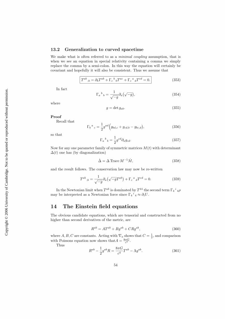
Cop

yrig

ht ©

200

6 U

nive

rsity

of C

ambr

idge

. Not

to b

e qu

oted

or

repr

oduc

ed w

ithou

t per

mis

sion

.

13.2 Generalization to curved spacetime

We make what is often referred to as a minimal coupling assumption, that iswhen we see an equation in special relativity containing a comma we simplyreplace the comma by a semi-colon. In this way the equation will certainly becovariant and hopefully it will also be consistent. Thus we assume that

T ab;b = ∂bT

ab + Γcb

bTac + Γc

adT

cd = 0. (353)

In fact

Γab

b =1√−g

∂a

(√−g)

, (354)

whereg = det gab. (355)

ProofRecall that

Γba

c =1

2gad

(

gbd,c + gcd,b − gbc,d

)

, (356)

so that

Γab

b =1

2gcd∂agcd. (357)

Now for any one parameter family of symmetric matrices M(t) with determinant∆(t) one has (by diagonalization)

∆ = ∆Trace M−1M, (358)

and the result follows. The conservation law may now be re-written

T ab;b =

1√−g∂a

(√−gT ab)

+ Γca

dTcd = 0. (359)

In the Newtonian limit when T ab is dominated by T 44 the second term Γ4i4ρ

may be interpreted as a Newtonian force since Γ4i4 ≈ ∂iU .

14 The Einstein field equations

The obvious candidate equations, which are tensorial and constructed from nohigher than second derivatives of the metric, are

Rab = AT ab + Bgab + CRgab, (360)

where A,B,C are constants. Acting with ∇a shows that C = 12 , and comparison

with Poissons equation now shows thatA = 8πGc4 .

Thus

Rab − 1

2gabR =

8πG

c4T ab − Λgab. (361)

54

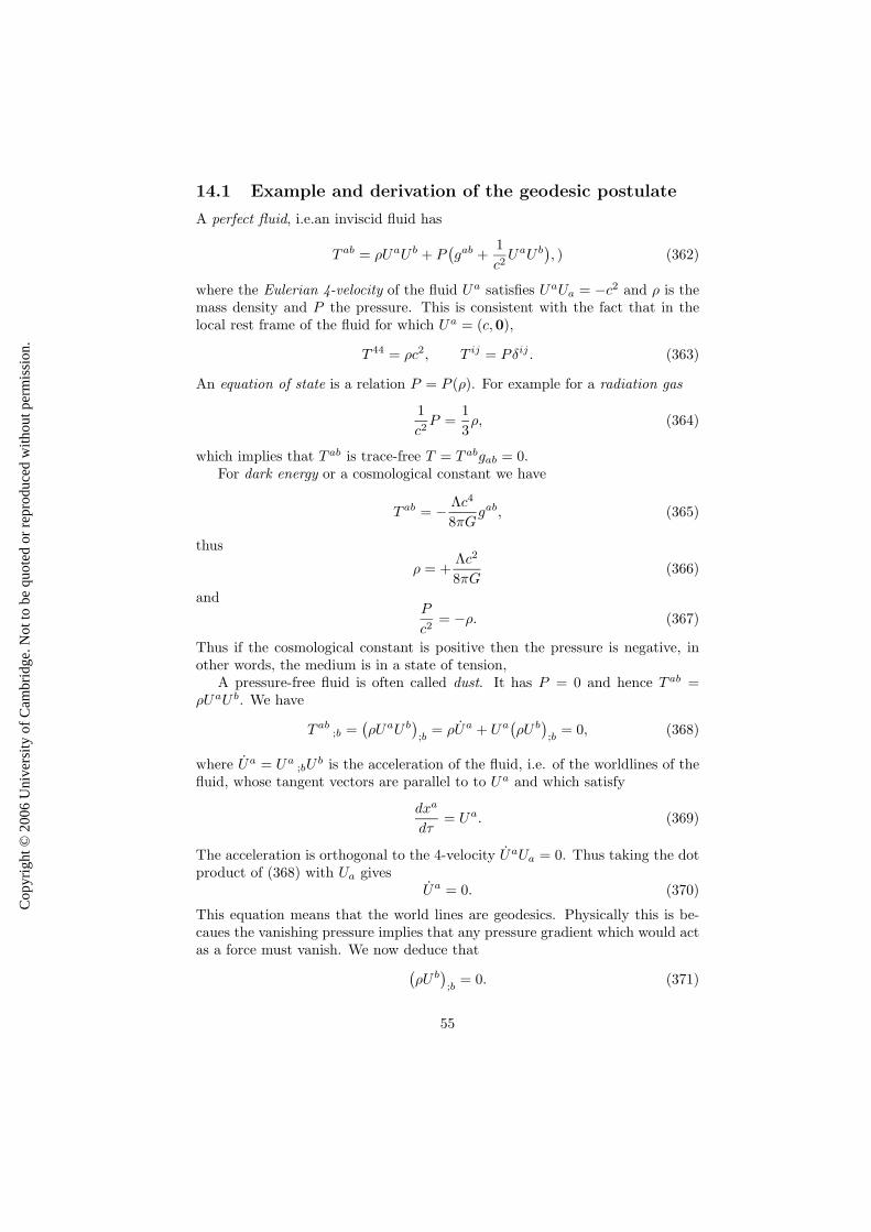
Cop

yrig

ht ©

200

6 U

nive

rsity

of C

ambr

idge

. Not

to b

e qu

oted

or

repr

oduc

ed w

ithou

t per

mis

sion

.

14.1 Example and derivation of the geodesic postulate

A perfect fluid, i.e.an inviscid fluid has

T ab = ρUaU b + P(

gab +1

c2UaU b

)

, ) (362)

where the Eulerian 4-velocity of the fluid Ua satisfies UaUa = −c2 and ρ is themass density and P the pressure. This is consistent with the fact that in thelocal rest frame of the fluid for which Ua = (c,0),

T 44 = ρc2, T ij = Pδij . (363)

An equation of state is a relation P = P (ρ). For example for a radiation gas

1

c2P =

1

3ρ, (364)

which implies that T ab is trace-free T = T abgab = 0.For dark energy or a cosmological constant we have

T ab = − Λc4

8πGgab, (365)

thus

ρ = +Λc2

8πG(366)

andP

c2= −ρ. (367)

Thus if the cosmological constant is positive then the pressure is negative, inother words, the medium is in a state of tension,

A pressure-free fluid is often called dust. It has P = 0 and hence T ab =ρUaU b. We have

T ab;b =

(

ρUaU b)

;b= ρUa + Ua

(

ρU b)

;b= 0, (368)

where Ua = Ua;bU

b is the acceleration of the fluid, i.e. of the worldlines of thefluid, whose tangent vectors are parallel to to Ua and which satisfy

dxa

dτ= Ua. (369)

The acceleration is orthogonal to the 4-velocity UaUa = 0. Thus taking the dotproduct of (368) with Ua gives

Ua = 0. (370)

This equation means that the world lines are geodesics. Physically this is be-caues the vanishing pressure implies that any pressure gradient which would actas a force must vanish. We now deduce that

(

ρU b)

;b= 0. (371)

55

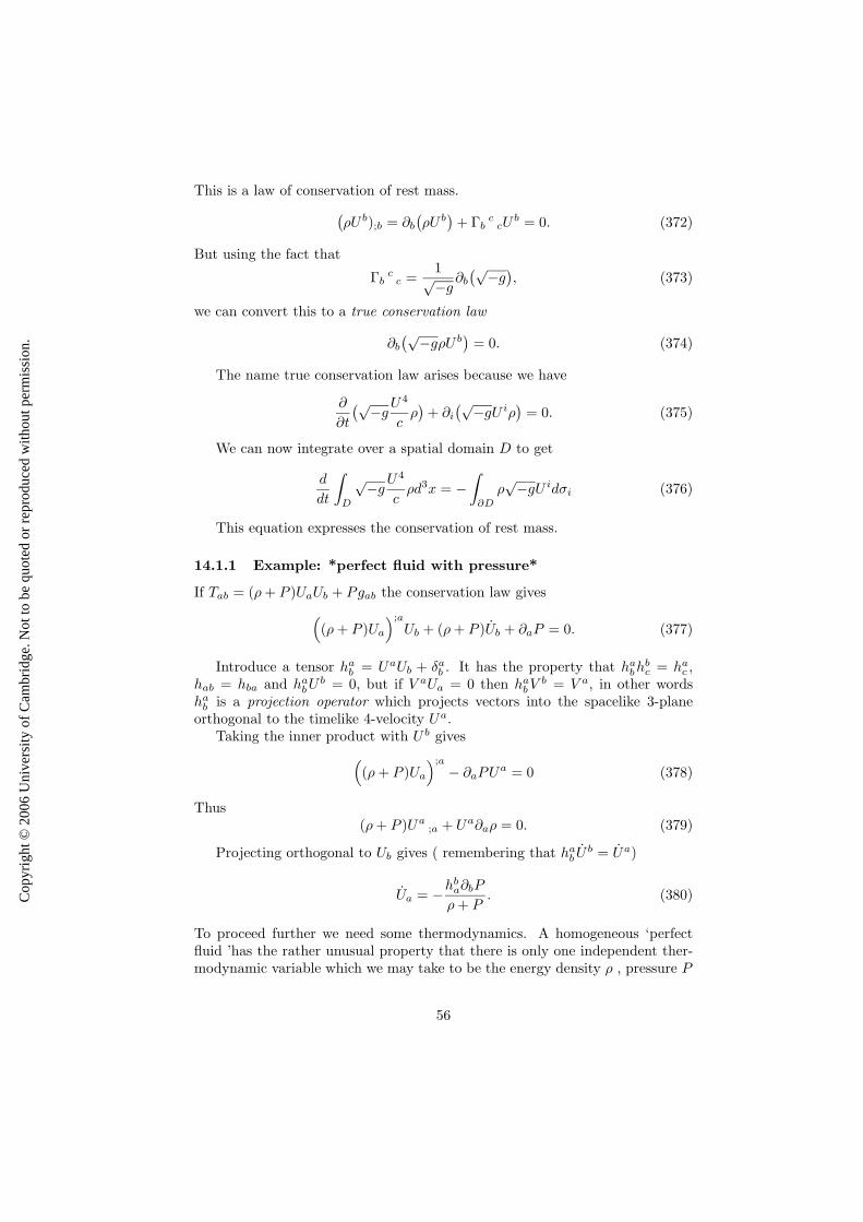
Cop

yrig

ht ©

200

6 U

nive

rsity

of C

ambr

idge

. Not

to b

e qu

oted

or

repr

oduc

ed w

ithou

t per

mis

sion

.

This is a law of conservation of rest mass.

(

ρU b);b = ∂b

(

ρU b)

+ Γbc

cUb = 0. (372)

But using the fact that

Γbc

c =1√−g

∂b

(√−g)

, (373)

we can convert this to a true conservation law

∂b

(√−gρU b)

= 0. (374)

The name true conservation law arises because we have

∂

∂t

(√−gU4

cρ)

+ ∂i

(√−gU iρ)

= 0. (375)

We can now integrate over a spatial domain D to get

d

dt

∫

D

√−gU4

cρd3x = −

∫

∂D

ρ√−gU idσi (376)

This equation expresses the conservation of rest mass.

14.1.1 Example: *perfect fluid with pressure*

If Tab = (ρ + P )UaUb + Pgab the conservation law gives

(

(ρ + P )Ua

);a

Ub + (ρ + P )Ub + ∂aP = 0. (377)

Introduce a tensor hab = UaUb + δa

b . It has the property that habhb

c = hac ,

hab = hba and habU b = 0, but if V aUa = 0 then ha

bV b = V a, in other wordsha

b is a projection operator which projects vectors into the spacelike 3-planeorthogonal to the timelike 4-velocity Ua.

Taking the inner product with U b gives

(

(ρ + P )Ua

);a

− ∂aPUa = 0 (378)

Thus(ρ + P )Ua

;a + Ua∂aρ = 0. (379)

Projecting orthogonal to Ub gives ( remembering that hab U b = Ua)

Ua = −hba∂bP

ρ + P. (380)

To proceed further we need some thermodynamics. A homogeneous ‘perfectfluid ’has the rather unusual property that there is only one independent ther-modynamic variable which we may take to be the energy density ρ , pressure P

56

Cop

yrig

ht ©

200

6 U

nive

rsity

of C

ambr

idge

. Not

to b

e qu

oted

or

repr

oduc

ed w

ithou

t per

mis

sion

.

, entropy density s or temperature T as we wish. They are linked by the firstlaw which reads

TdS = dU + PdV (381)

Now for a homogeneous substance, if U = V ρ, S = sV , this gives

Tds = dρ (382)

andTs = ρ + P. (383)

The latter formula is sometimes called the Gibbs-Duhem relation. It follows that

ds

s=

dρ

ρ + P. (384)

Thus we may re-write (379) as the law of entropy conservation

(

sUa)

;a= 0. (385)

To understand the other equation we note that

dP

ρ + P=

dT

T. (386)

Thus

Ua = −hba∂bT

T. (387)

For a fluid at rest in a static metric,

Ua =(

0, ∂i ln(√−g44)

)

(388)

and hence∂i ln(

√−g44) = −∂i lnT (389)

thusT√−g44 = constant, (390)

which is called Tolman’s redshift law. A gas in equilibrium in a static gravita-tional potential must have a temperature which increases as the gravitationalpotential decreases by precisely the redshift factor.If this were not so one couldconstruct a perpetual motion machine by converting the local energy at highpotential into thermal photons and sending them to a location of lower poten-tial. The photons would gain energy and have the redshifted temperature. Ifthis were not equal to the local value, the temperature difference could be usedto do work.

57

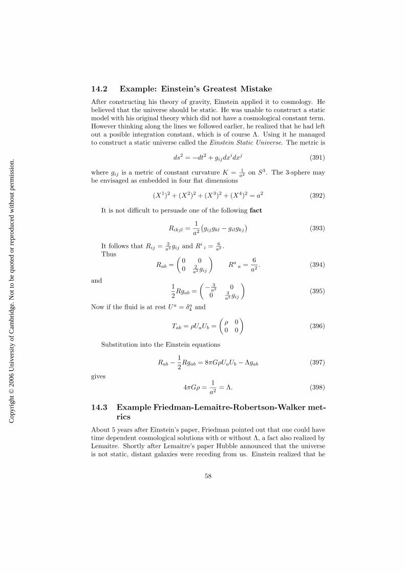
Cop

yrig

ht ©

200

6 U

nive

rsity

of C

ambr

idge

. Not

to b

e qu

oted

or

repr

oduc

ed w

ithou

t per

mis

sion

.

14.2 Example: Einstein’s Greatest Mistake

After constructing his theory of gravity, Einstein applied it to cosmology. Hebelieved that the universe should be static. He was unable to construct a staticmodel with his original theory which did not have a cosmological constant term.However thinking along the lines we followed earlier, he realized that he had leftout a posible integration constant, which is of course Λ. Using it he managedto construct a static universe called the Einstein Static Universe. The metric is

ds2 = −dt2 + gijdxidxj (391)

where gij is a metric of constant curvature K = 1a2 on S3. The 3-sphere may

be envisaged as embedded in four flat dimensions

(X1)2 + (X2)2 + (X3)2 + (X4)2 = a2 (392)

It is not difficult to persuade one of the following fact

Rikjl =1

a2

(

gijgkl − gilgkj

)

(393)

It follows that Rij = 2a2 gij and Ri

i = 6a2 .

Thus

Rab =

(

0 00 2

a2 gij

)

Raa =

6

a2. (394)

and1

2Rgab =

(

− 3a2 00 3

a2 gij

)

(395)

Now if the fluid is at rest Ua = δa4 and

Tab = ρUaUb =

(

ρ 00 0

)

(396)

Substitution into the Einstein equations

Rab −1

2Rgab = 8πGρUaUb − Λgab (397)

gives

4πGρ =1

a2= Λ. (398)

14.3 Example Friedman-Lemaitre-Robertson-Walker met-rics

About 5 years after Einstein’s paper, Friedman pointed out that one could havetime dependent cosmological solutions with or without Λ, a fact also realized byLemaitre. Shortly after Lemaitre’s paper Hubble announced that the universeis not static, distant galaxies were receding from us. Einstein realized that he

58

Cop

yrig

ht ©

200

6 U

nive

rsity

of C

ambr

idge

. Not

to b

e qu

oted

or

repr

oduc

ed w

ithou

t per

mis

sion

.

had failed to make this a prediction of his theory, and alledgedly refered to hisintroduction of Λ as the greatest blunder of his life. Blunder or not, it hasno re-surfaced as vacuum energy, and seems to dominate the expansion of theuniverse. To see how we consider the metric

ds2 = −dt2 + a2(t)gij(xk)dxidxj (399)

where now the spatial metric is taken to be a 3-sphere of radius√

k, k = 0, 1.The case k = −1 is also allowed.

A straightforward but tiresome calculation shows that the Einstein equationsreduce to

(i)a

a= −4πG

3ρ +

Λ

3(400)

(ii)a2

a2+

k

a2=

8πGρ

3+

Λ

3(401)

(iii) ρ +3a

aρ = 0. (402)

15 Spherically Symmetric vacuum metrics

We start by establishing

Birkhoff’s Theorem The unique spherically symmetric vacuum metric is (lo-cally) the Static Schwarzschild metric

ds2 = −(

1 − 2GM

r

)

dt2 +dr2

1 − 2GMr

+ r2(

dθ2 sin2 θdφ2)

(403)

This generalizes Newton’s theorem and greatly simplifies the study of gravi-ational collapse. Any spherically symmetric source, e.g. a pulsating, exploding,or collapsing star has an exterior metric exactly given by the Schwarzschild met-ric. Physically this can be understood in part from the fact that gravitationalwaves are transverse and polarizable. Any polarization would define a directionfield on S2 but by the Hairy Ball Theorem it cannot therefore be sphericallysymmetric.

ProofStep 1: The metric The meric may be cast in the form

ds2 = A(r, t)dt2 + 2B(r, t)drdt + C(r, t)dr2 + R2(r, t)(

dθ2 + sin2 θdφ2)

(404)

There can be no gaθ or gaφ terms with a = r, t by spherical symmetry. Weare still allowed to change the coordinates r, t

r → r = r(r, t), t → t = t(r, t). (405)

59

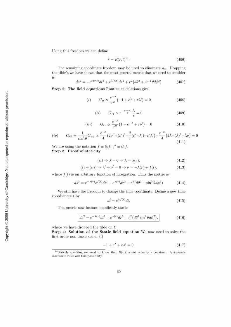
Cop

yrig

ht ©

200

6 U

nive

rsity

of C

ambr

idge

. Not

to b

e qu

oted

or

repr

oduc

ed w

ithou

t per

mis

sion

.

Using this freedom we can define

r = R(r, t)14. (406)

The remaining coordinate freedom may be used to eliminate grt. Droppingthe tilde’s we have shown that the most general metric that we need to consideris

ds2 = −eν(r,t)dt2 + eλ(r,t)dr2 + r2(

dθ2 + sin2 θdφ2)

(407)

Step 2: The field equations Routine calculations give

(i) Gtt ∝e−λ

r2

(

−1 + eλ + rλ′)

= 0 (408)

(ii) Grt ∝ e−(ν+λ)

2λ

r= 0 (409)

(iii) Grr ∝ e−λ

r2

(

1 − e−λ + rν′)

= 0 (410)

(iv) Gθθ =1

sin2 θGφφ ∝ e−λ

4

(

2ν′′+(ν′)2+2

r(ν′−λ′)−ν′λ′

)

−e−ν

4

(

2λ+(λ)2−λν)

= 0

(411)We are using the notation f ≡ ∂tf, f ′ ≡ ∂rf .Step 3: Proof of staticity

(ii) ⇒ λ = 0 ⇒ λ = λ(r). (412)

(i) + (iii) ⇒ λ′ + ν′ = 0 ⇒ ν = −λ(r) + f(t), (413)

where f(t) is an arbitrary function of integration. Thus the metric is

ds2 = e−λ(r)ef(t)dt2 + eλ(r)dr2 + r2(

dθ2 + sin2 θdφ2)

(414)

We still have the freedom to change the time coordinate. Define a new timecoordianate t by

dt = e12 f(t)dt. (415)

The metric now bcomes manifestly static

ds2 = e−λ(r)dt2 + eλ(r)dr2 + r2(

dθ2 sin2 θdφ2)

, (416)

where we have dropped the tilde on t.Step 4: Solution of the Static field equation We now need to solve thefirst order non-linear o.d.e. (i)

−1 + eλ + rλ′ = 0. (417)

14Strictly speaking we need to know that R(r, t)is not actually a constant. A separatediscussion rules out this possibility

60

Cop

yrig

ht ©

200

6 U

nive

rsity

of C

ambr

idge

. Not

to b

e qu

oted

or

repr

oduc

ed w

ithou

t per

mis

sion

.

This can be done by making the substitution

e−λ = 1 + D(r), (418)

to getD′

D= −1

r. (419)

The solution is

D = −2M

r, (420)

where M is an arbitrary integration constant.

16 Geodesics in the Schwarzschild metric

Without loss of generality we can set θ = π2 . The Lagrangian becomes

L = −(

1 − 2M

r

)

( dt

dλ

)2

+1

1 − 2Mr

( dr

dλ

)2

+ r2(dφ

dλ

)2

. (421)

Since L is independent of λ, Noether’s theorem gives

(i)(

1 − 2M

r

)

( dt

dλ

)2

− 1

1 − 2Mr

( dr

dλ

)2

− r2(dφ

dλ

)2

= k, (422)

where k = +1, 0,−1 for timelike, lightlike or spacelike geodesics respectively.Since L is independent of t Noether’s theorem gives

(ii)(

1 − 2M

r

)

( dt

dλ

)

= E, (423)

where E is the energy (per unit mass in the timelike case). Since L is indepen-dent of φ Noether’s theorem gives

(iii) r2(dφ

dλ

)

= h, (424)

where h is the angular momentum (per unit mass in the timelike case). Substi-tution of (ii) and (iii) in (i) gives

( dr

dλ

)2

= E2 −(

1 − 2M

r

)(

k +h2

r2

)

. (425)

16.1 The shape of the orbit

Using (iii) we get

h2

r2

( dr

dφ

)2

= E2 −(

1 − 2M

r

)(

k +h2

r2

)

. (426)

61

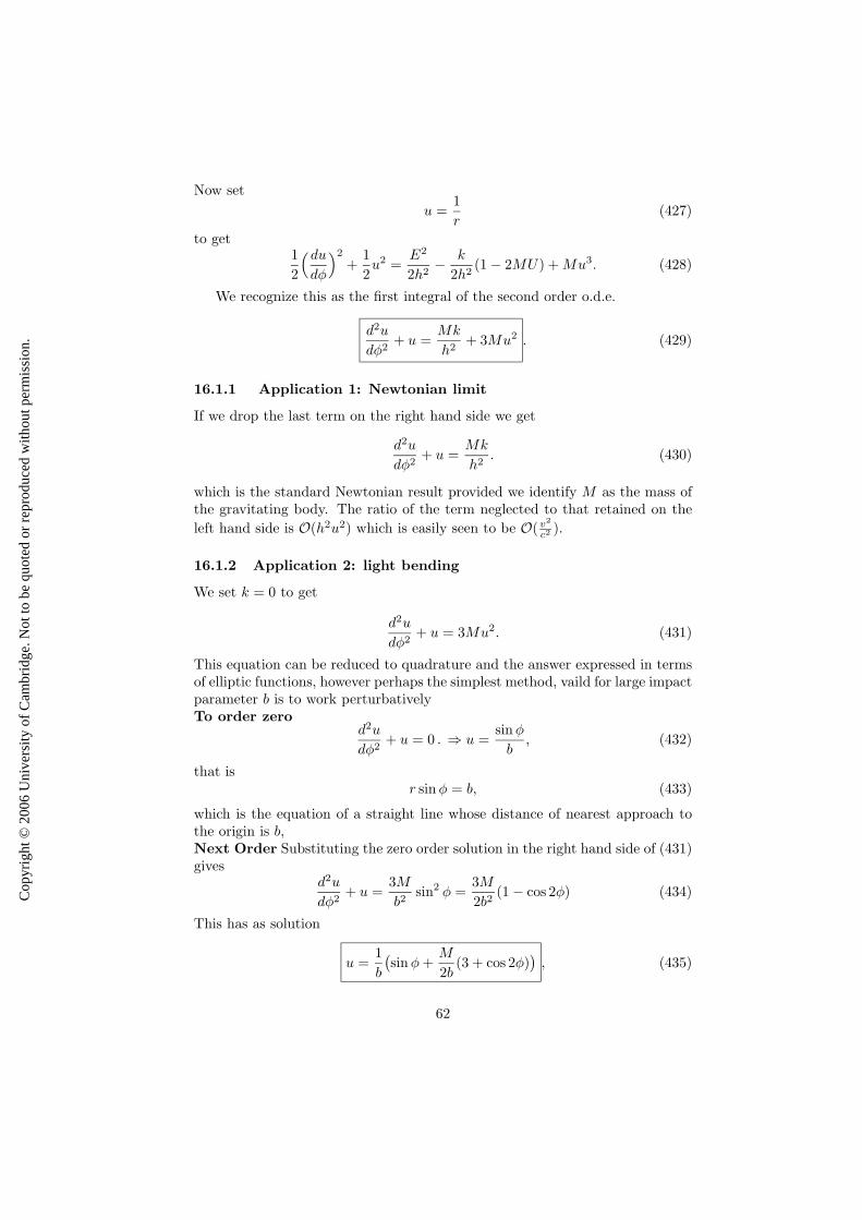
Cop

yrig

ht ©

200

6 U

nive

rsity

of C

ambr

idge

. Not

to b

e qu

oted

or

repr

oduc

ed w

ithou

t per

mis

sion

.

Now set

u =1

r(427)

to get1

2

(du

dφ

)2

+1

2u2 =

E2

2h2− k

2h2(1 − 2MU) + Mu3. (428)

We recognize this as the first integral of the second order o.d.e.

d2u

dφ2+ u =

Mk

h2+ 3Mu2 . (429)

16.1.1 Application 1: Newtonian limit

If we drop the last term on the right hand side we get

d2u

dφ2+ u =

Mk

h2. (430)

which is the standard Newtonian result provided we identify M as the mass ofthe gravitating body. The ratio of the term neglected to that retained on the

left hand side is O(h2u2) which is easily seen to be O(v2

c2 ).

16.1.2 Application 2: light bending

We set k = 0 to get

d2u

dφ2+ u = 3Mu2. (431)

This equation can be reduced to quadrature and the answer expressed in termsof elliptic functions, however perhaps the simplest method, vaild for large impactparameter b is to work perturbativelyTo order zero

d2u

dφ2+ u = 0 . ⇒ u =

sin φ

b, (432)

that isr sinφ = b, (433)

which is the equation of a straight line whose distance of nearest approach tothe origin is b,Next Order Substituting the zero order solution in the right hand side of (431)gives

d2u

dφ2+ u =

3M

b2sin2 φ =

3M

2b2(1 − cos 2φ) (434)

This has as solution

u =1

b

(

sin φ +M

2b(3 + cos 2φ)

)

, (435)

62

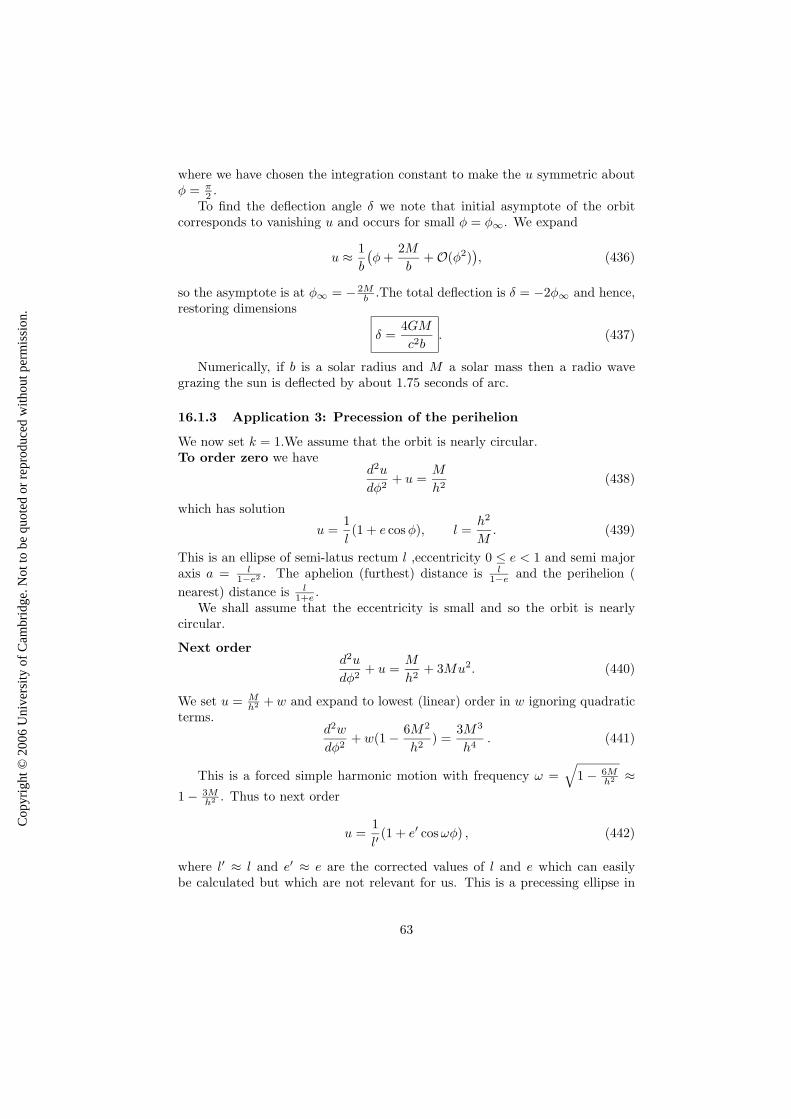
Cop

yrig

ht ©

200

6 U

nive

rsity

of C

ambr

idge

. Not

to b

e qu

oted

or

repr

oduc

ed w

ithou

t per

mis

sion

.

where we have chosen the integration constant to make the u symmetric aboutφ = π

2 .To find the deflection angle δ we note that initial asymptote of the orbit

corresponds to vanishing u and occurs for small φ = φ∞. We expand

u ≈ 1

b

(

φ +2M

b+ O(φ2)

)

, (436)

so the asymptote is at φ∞ = − 2Mb

.The total deflection is δ = −2φ∞ and hence,restoring dimensions

δ =4GM

c2b. (437)

Numerically, if b is a solar radius and M a solar mass then a radio wavegrazing the sun is deflected by about 1.75 seconds of arc.

16.1.3 Application 3: Precession of the perihelion

We now set k = 1.We assume that the orbit is nearly circular.To order zero we have

d2u

dφ2+ u =

M

h2(438)

which has solution

u =1

l(1 + e cos φ), l =

h2

M. (439)

This is an ellipse of semi-latus rectum l ,eccentricity 0 ≤ e < 1 and semi majoraxis a = l

1−e2 . The aphelion (furthest) distance is l1−e

and the perihelion (

nearest) distance is l1+e

.We shall assume that the eccentricity is small and so the orbit is nearly

circular.

Next orderd2u

dφ2+ u =

M

h2+ 3Mu2. (440)

We set u = Mh2 + w and expand to lowest (linear) order in w ignoring quadratic

terms.d2w

dφ2+ w(1 − 6M2

h2) =

3M3

h4. (441)

This is a forced simple harmonic motion with frequency ω =√

1 − 6Mh2 ≈

1 − 3Mh2 . Thus to next order

u =1

l′(1 + e′ cos ωφ) , (442)

where l′ ≈ l and e′ ≈ e are the corrected values of l and e which can easilybe calculated but which are not relevant for us. This is a precessing ellipse in

63

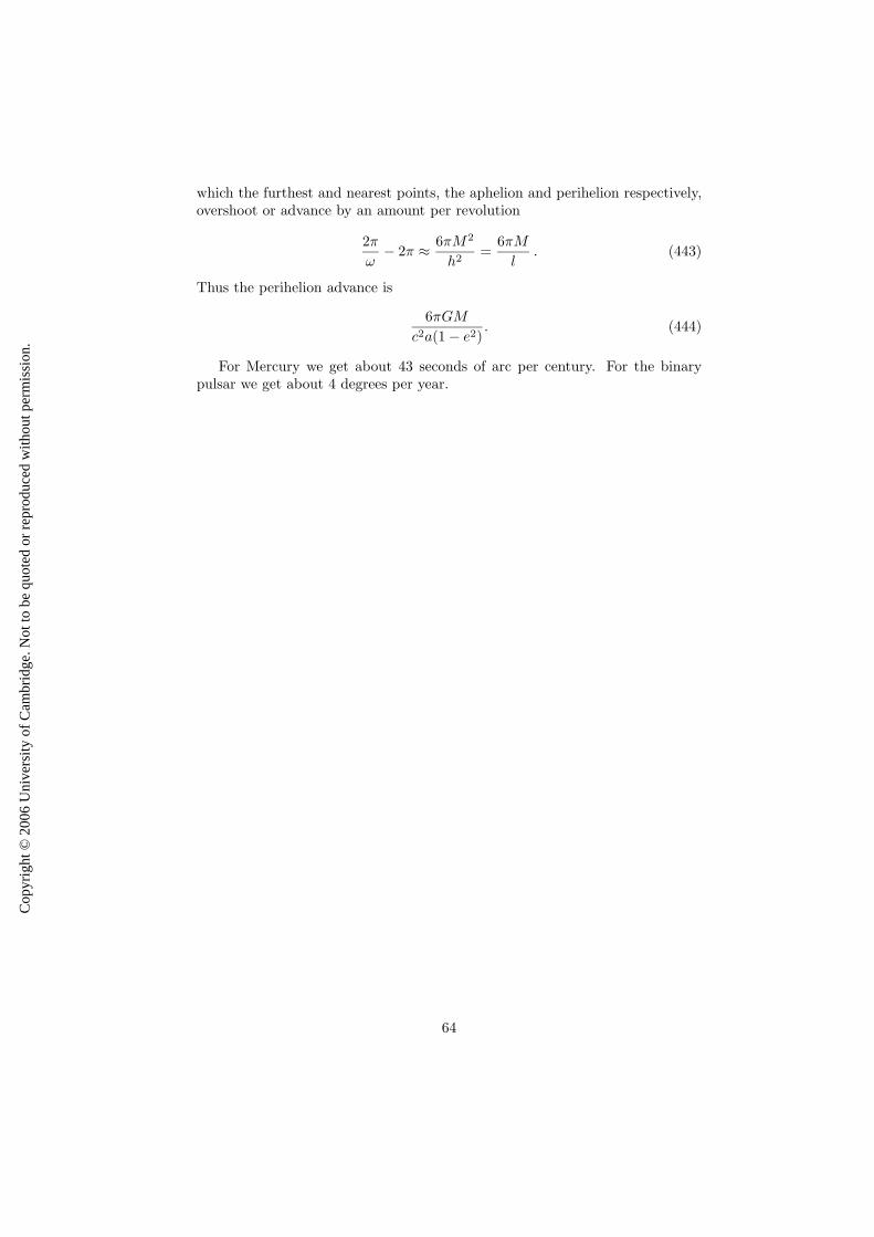
Cop

yrig

ht ©

200

6 U

nive

rsity

of C

ambr

idge

. Not

to b

e qu

oted

or

repr

oduc

ed w

ithou

t per

mis

sion

.

which the furthest and nearest points, the aphelion and perihelion respectively,overshoot or advance by an amount per revolution

2π

ω− 2π ≈ 6πM2

h2=

6πM

l. (443)

Thus the perihelion advance is

6πGM

c2a(1 − e2). (444)

For Mercury we get about 43 seconds of arc per century. For the binarypulsar we get about 4 degrees per year.

64