H

PARALLEL FLUID DYNAMICS COMPUTATIONS IN AEROSPACE APPLICATIONS

S. K. ALIABADI AND T. E. TEZDUYAR Department of Aerospace Engineering and Mechanics and Army High Pe$ormance Computing Research Center:

Universiiy of Minnesota, 1100 Washington Avenue South, Minneapolis, MN 55415. US.A.

SUMMARY

Massively parallel finite element computations of the compressible Euler and Navier-Stokes equations using parallel supercomputers are presented. The finite element formulations are based on the conservation variables and the streamline-upwind/Petrov-Galerkin (SUPG) stabilization method is used to prevent potential numerial oscillations due to dominant advection terms. These computations are based on both implicit and explicit methods and their parallel implementation assumes that the mesh is unstructured. The implicit computations are based on iterative strategies. Large-scale 3D problems are solved using a matrix-free iteration technique which reduces the memory requirements significantly. The flow problems we consider typically come from aerospace applications, including those in 3D and those involving moving boundaries interacting with boundary layers and shocks. Problems with fixed boundaries are solved using a semidiscrete formulation and the ones involving moving boundaries are solved using the deformable-spatial-domaidstabilized-space-time (DSD/SST) formulation.

KEY WORDS: parallel finite elements; 3D compressible flows; stabilized method; space-time method

1. INTRODUCTION

The aerodynamic characteristics of new design concepts in the aerospace industry are usually measured in wind tunnels. When using a wind tunnel as a design tool, engineers are required to go through the expensive and time-consuming process of building a precise physical model and subjecting it to several costly experiments. Any modification to the design configuration demands a new model and experimental data.

Computational fluid dynamics (CFD) offers a way to partially replace costly, time-consuming and difficult wind tunnel tests. CFD entered the industry almost two decades ago. At that time it was only possible to simulate simple 1D time-dependent problems. The advent of the first series of Cray-family supercomputers in the early 1980s contributed to the power of CFD and enabled designers and researchers to model transient problems in 2D. In some cases a simple steady state application in 3D was simulated, but this computational power was still far from what was needed in the aerospace industry in order to partially replace experiments in wind tunnels.

Performance enhancements of single-processor supercomputers improved asymptotically in the late 1980s and reached a certain point where further improvement seemed very difficult. These machines are based on a single-instructiodsingle-data (SISD) architecture and their performance is limited by the material properties of the computer chips. Consequently, the need for an alternative computer architecture emerged. The subsequent development of supercomputers focused on parallel machines with single-instructiodmultiple-data (SIMD) or multiple-instructiodmultiple-data (MIMD) architec- tures.

CCC 0271-2091J95J100783-23 0 1995 by John Wiley & Sons, Ltd.

Received 24 July I994 Revised 22 August 1994

784 S. K. ALIABADI AND T. E. TEZDUYAR

Today there are many parallel supercomputers built based on either the SIMD or the MIMD structure. The MasPar MP-2 and the Connection Machine CM-200 are examples of the SIMD structure, while the nCUBE 2E, the Cray T3D and the Connection Machine CM-5 are massively parallel supercomputers with an MIMD architecture. The CM-5 can also operate in SIMD mode. These supercomputers have computational power which allows researchers to simulate 3D time- accurate fluid flow problems. Today we are at a stage where the steady state solution of a Euler flow past an entire aeroplane can be obtained in just a few minutes. This computational power is still not enough to understand the physics of some real-life applications. As computers advance towards teraFLOPS (trillion floating point operations per second) speeds by the end of this century, they will play a significant role in the design, manufacturing and control system processes in industry. Developing robust, accurate, efficient and simple algorithms to handle these tasks is a continuing challenge.

In this paper we present finite element methods to solve a large class of compressible flow problems using the Connection Machine massively parallel supercomputers CM-200 and CM-5. In Section 2 we first review the governing equations of compressible fluid mechanics and heat transfer. Two sets of equations, Euler and Navier-Stokes, are used to model the compressible flow field in our problems. For the compressible Navier-Stokes equations we assume that the fluid is Newtonian and that the heat transfer by conduction is modelled by Fourier's law.

The solution of problems with fixed domains is obtained using a semidiscrete formulation. This finite element formulation is stated in the context of the conservation variables and the potential for

es in high-inertia flows is prevented using the streamline-upwindPetrov-Galerkin (SUPG) stabilization method. The Galerkin method by itself is inherently a central difference scheme and it is well known that central difference schemes lack stability and result in node-to-node spurious oscillations in advection-dominated flows. The SUPG method is a general weighted-residual upwinding scheme which minimizes such oscillations and preserves consistency. The SUPG formulation was first developed by Hughes and Brooks' for incompressible flows. A comprehensive description of the formulation, together with various numerical examples, can be found in Reference 2.

For the Euler equations, the SUPG method was first developed by Tezduyar and H~gHes.~ Using the entropy variables, a similar stabilized formulation with an in-built shock-capturing term was developed later.4" It was shown that the entropy variable formulation is more robust than the conservation variable formulation in solving problems involving shocks and sharp boundary layers. Recently Le Beau and Tezduyar7 and Le Beau et al.' incorporated a shock-capturing term into the conservation variable formulation and demonstrated that this formulation generates solutions with as a high quality as those obtained with the entropy variable formulation.

The simplicity of the conservation variable formulation compared with the entropy variable formulation motivated us to extend the formulation further and apply it to the Navier-Stokes equations. The results from this effort were first reported by Aliabadi et aL9 and followed by many examples in References 1&12. In Section 3 we present the semidiscrete formulation following the stabilization details.

Section 4 is devoted to describing the time integration techniques for solving the coupled non- linear ordinary differential equation systems resulting from the semidiscrete formulation. These equations are solved within the framework of the predictor/multicorrector algorithm by using either explicit or implicit techniques. The implicit computations are carried out with an iterative solution of the coupled linear equation systems encountered at each step of the predictor/multicorrector algorithm. Large-scale 3D problems are solved using matrix-free iterations which are also described briefly in this section.

A major challenge in computational fluid dynamics is how to handle problems involving moving boundaries and interfaces. These kinds of problems are encountered in many practical engineering

PARALLEL FLUID DYNAMICS COMPUTATIONS 785

applications. In manufacturing, almost all processes such as casting, rolling, extrusion, forging and pressing involve moving boundaries. Fluid-structure interactions are another area where moving boundaries play an important role. A few examples in this category are the movement of aircraft control surfaces, flutter phenomena, moving mechanical parts interacting with fluids and opening of a ram air parachute. The semidiscrete formulation is based on a Eulerian approach. In the Eulerian approach the spatial domain is fixed. To handle problems in which the spatial domain deforms, the Eulerian approach may be mixed with the Langrangian approach, resulting in the arbitrary Langrangian-Eulerian (ALE) method (see References 13-1 6 for details).

The deformable-spatial-domaidstabilized space-time (DSD/SST) finite element formulation is another approach which can be used to address the issue of moving boundaries and interfaces. This method was introduced by Tezduyar et al. 1 7 , 1 8 to solve incompressible flow problems involving moving boundaries and interfaces such as free surfaces, two-liquid interfaces and fluid-structure and fluid-particle interactions. Later a similar formulation was developed for compressible flows." In the DSD/SST formulation, the finite element interpolation polynomials are functions of both space and time and the stabilized variational formulation of the problem is written over the associated space-time domain. These interpolation polynomials are continuous in the spatial domain but discontinuous in time. The discontinuous interpolation polynomials in time allow the solution of the discrete equations at each time step. By taking advantage of the space-time approach, the DSD/SST formulation is inherently able to take into account the deformation of the spatial domain with respect to time. This formulation is described in Section 5.

In Section 6 several numerical examples are presented to illustrate the application of these methods. Final remarks and the performance of our computations on the CM-200 and CM-5 are given in

Section 7.

2. GOVERNING EQUATIONS

Let Sl, c [w"" and (0, T ) be the spatial and temporal domains respectively, where nsd is the number of space dimensions, and let Tt denote the boundary of R,. The spatial and temporal co-ordinates are denoted by x and t respectively. We consider the 3D unsteady compressible Navier-Stokes equations without source terms. These equations in conservation law form can be written as

(1) aP - + V * (up) = 0 on Q, Vt E (0, T ) , at

a O + V . ( u p u ) at = - -Vp+V.T on Q,

(3) -+V. (upe)=-V*q-V.pu+V. (Tu) a(Pe> on, V t E ( 0 , T ) .

at

Here p(x, t), u(x, t), p(x, t) and e(x, t ) are the density, velocity, pressure and total energy per unit mass respectively. The viscous stress tensor and heat flux vector are denoted by T and q respectively. The pressure is related to the other state variables by an equation of state of the form

P =P(P, 9, (4)

786

where

S. K. ALIABADI AND T. E. TEZDUYAR

is the internal energy. For ideal gases the equation of state takes the special form

p = (Y - 1)pC

T = p[Vu + ( V U ) ~ ] + I(V*u)I,

(6)

where y is the ratio of specific heats. The viscous stress tensor T and heat flux vector q are defined as

(7)

q = -Kve, (8)

where K is the conductivity and 8 is the temperature with the following relationship to the internal energy:

Ri e x - , Y-1

(9)

Here R is the ideal gas constant and it is assumed that the viscosity coefficients y and p are related by

(10) y = -2 3 p.

The variation in the viscosity with temperature is modelled by Sutherland's empirical formula (3 3/2 er + eo e + e o P = Pr

where Oo is an experimentally determined constant and pr is the viscosity at the reference temperature OF The Prandtl number Pr, assumed to be given, relates the heat conductivity to the viscosity according to

In terms of conservation variables the compressible Navier-Stokes equations ( 9 4 3 ) can be written in the vector form

au aF; aEi at ax; ax;

- + - - - = O o n Q V t e ( O , T ) ,

where U = (p , pul , pu2, pu3, pe) is the vector of conservation variables and Fi and Ei are respectively the Euler and viscous flux vectors defined as

F; =

PARALLEL FLUID DYNAMICS COMPUTATIONS 787

Here uj, qs and z~~ are the components of the velocity, heat flux and viscous stress tensor respectively, repeated indices imply summation Over the range of the spatial dimension and the identity tensor is denoted by 6,.

To provide a convenient set-up for our finite formulations, equation (1 3) is written in the form

where

is the Euler Jacobian matrix and K, is the diffisivity matrix satisfying

The explicit definitions of Ai and K, are provided in the Appendix. Equation (16) is complemented with initial and boundary conditions of the form

U(X, 0) = uo, (19)

where ek is an orthonormal basis function in R""', and ndof is the number of degrees of freedom. Note that the Euler equations can be obtained by dropping the diffusive terms from equation (1 6).

3. SEMIDISCRETE FINITE ELEMENT FORMULATION

Consider a finite element discretization of a fixed spatial domain R into subdomains Re, e = 1, 2, . . . , riel, where n,l is the number of elements. Based on the discretization, corresponding to the trial solutions and weighting hnctions respectively, we define the finite element function spaces Yh and V h for conservation variables. These function spaces are selected as subsets of [H'h(S2)]n"f, where Hlh{12) is the finite-dimensional function space over 0

Yh = (uhluh E [H'h(s2)J"do', Uh1ne E [P'(fie)lndof, uh 'ek=gk On JJ,,), (22)

788 S. K. ALIABADI AND T. E. TEZDUYAR

The stabilized finite element formulations of (16) is written as follows: find Uh E Y h such that V W h E V h

In the variational formulation given by (24), the first two terms together with the right-hand-side term constitute the Galerkin formulation of the problem. The first series of element-level integrals in (24) are the SUPG stabilization terms added to the variational formulation to prevent spatial oscillations in the advection-dominated range. The second series of element-level integrals in (24) are the shockkapturing terms added to the formulation to ensure stability at high Mach and Reynolds numbers.

In this work we propose a 7 which evolves from the one introduced by Tezduyar and hug he^.^ We define the SUPG stabilization matrix 7 to be

7 - max[O, T~ + 5 ( ~ ~ - ~g - ?do], (25)

where I , is the stabilization matrix due to the time-dependent term, is the stabilization matrix due to the advection terms, ~g and ?d are the matrices subtracted from T, to account for the presence of the shock-capturing term and physical diffusion respectively and 5 is the weighting coefficient. These matrices are defined as

rn L

3(1 + 2aCr)'" Tt =

h 7 -

a - 2(c + lu. PI)I'

(c + lu - P,I2 I, 6

7 g =

B?diagK11 + &diagKtz + PidiagK33 Td =

(c + lu * PD2

(c + lu * P W where c is the acoustic speed, Cr is the Courant number given by

h Cr =

and h is the element length. Here

where 4 - l is the inverse of the Reimannian metric t e n ~ o r . ~ For the time-marching algorithm the weighting coefficient [ is selected as

2aCr [ = 1 +2CrCr' (33)

PARALLEL FLUID DYNAMICS COMPUTATIONS 789

where tl is a parameter which governs the stability and accuracy of the algorithm (see next section). The shock-capturing parameter 6 used in this formulation is given as7

where 4 k are the components of the Jacobian transformation matrix from physical to local co-ordinates. The structure of 6 is such that it vanishes rapidly in the regions where the solution is smooth and is significant in the regions with sharp boundary layers and shocks.''

4. TIME INTEGRATION METHODS

The spatial discretization of equation (24) leads to a set of coupled non-linear ordinary differential equations of the form

Ma + N(v) = F, (35) where v is the vector of nodal values of U, a is its time derivative, M is the generalized 'mass' matrix, N is the non-linear vector function of v representing the terms from the steady state equations and F is the generalized 'force' vector. To solve this equation system, we use the predictor/multicorrector transient algorithm described in Reference 3. In this algorithm the equation is temporally discretized in a finite difference fashion. The time-marching procedure is then performed by looping over the discrete time steps t,. With n as the time step represented by a,, v, and F, respectively. The steps. Given v, and a,:

1. Predictor phase

(a) i=O (b) predict a

2. Corrector phase

(a) compute R = F,+ - [Mii+N(V)] (b) select M (c) solve MAa=R (d) update a,+1 = a+Aa (e) update v,+~ = V+aAtAa (f) i= i+l ; V=V,+~; a=a,+l.

(c) V == v,+(l- a)Ata,+aAta.

counter, approximations to a(&), v(tn) and F(t,) are algorithm can then be summarized in the following

Here tl E [0, 11 is a parameter which governs the stability and accuracy of the method. To obtain a steady state solution using this predictor/multicorrector transient algorithm, a is set to one. In this case the algorithm is a backward difference type. When a = 0.5, the algorithm is second-order accurate in time and suitable for time-accurate computations. The fully explicit algorithm may be obtained by assigning a= 0 (forward difference). The details of the stability and accuracy of the algorithm can be found in Reference 2 1.

In the predictor/multicorrector algorithm the non-linear iteration loop starts in the corrector phase. In this loop the additional non-linear iterations are performed by replacing i with i + 1 and the calculations resume with the evaluation of the residual vector. This loop continues until the

790 S. K. ALIABADI AND T. E. TEZDUYAR

normalized L2-normal of the residual vector satisfies the convergence criteria. The solution at time step n+l is defined by the last iteration. Depending on the selection of M, this algorithm leads to an explicit or implicit time integration method.

4.1. Explicit method

In the explicit method, M is selected as a diagonal matrix. There are several ways to select an appropriate diagonal matrix M. In the present work we select M to be a lumped mass m a t r i ~ . ~ The simplicity of the inversion of a diagonal matrix makes the algorithm fast and inexpensive. The penalty for this is the time step size limitation governed by the Courant-Friedrichs-Lavy (CFL) condition. For the compressible Navier-Stokes equations this condition can be expressed as22

Despite this time step size limitation, this explicit method is particularly suitable for time-accurate computations. This is because in time-accurate computations, limitations on the time step size already exist owing to the need to accurately resolve the time-dependent behaviour.

4.2. Implicit method

In the implicit method, M is defined as

M = M + UAtC. (37)

Here M is no longer a diagonal matrix and therefore the coupled linear equations must be solved with either a direct or an iterative method.

Although M has a symmetric profile, in general, it is a non-symmetric matrix and this precludes the use of fast direct symmetric solution techniques. The commonly used non-symmetric direct solution techhniques are the Gaussian elimination and Crout factorization methods.

All direct methods require the global formation of M. Most entries of this matrix are zero, because each node in the mesh is connected only to a few nearby nodes. This matrix is usually stored in a skyline profile23 to minimize the memory requirements. In this way the number of stored entries is bN, where b is the mean bandwidth and the size of M is N x N. In many cases the mean bandwidth can be reduced by reordering the node numbering. The reordering is especially helpfd in cases when the mesh is generated using an automatic mesh generator.24

When a linear system has a large number of unknowns, direct methods become unwieldy. The major drawback of these methods is the memory requirement for storage. For large problems the memory requirements become very high and this makes the application of these methods, even on the advanced supercomputers with gigabyes of memory, impossible. Another disadvantage of these methods is the rapid increase in the number of arithmetic operations with the problem size. For example, in the Gaussian elimination method the number of arithmetic operations is proportional to Nb2. Thus the time required for the solution of a linear system by the Gaussian elimination method rapidly increases as the number of unknowns increases. These undesirable properties limit the application of these methods to small problems.

In most practical cases, even with the advanced supercomputers, the iterative methods are the only choices to solve large systems of coupled equations. In finite element computations, iterations can be performed without the need for the global formation of M. Also, in most of these iterative methods the number of arithmetic operations scales linearly with the problem size. Unlike the direct methods, the

PARALLEL FLUID DYNAMICS COMPUTATIONS 79 1

iterative methods are also naturally amenable to parallel processing. In the computations reported in this paper, iterations are carried out by using an appropriate preconditioner together with the GMRES2s326 search technique.

The iterations require matrix-vector multiplications of the form BY. Clearly, to perform this multiplication, matrix B need not be formed globally. Instead, this multiplication is performed by recognizing that

&I

e= 1 B = A b e ,

where f=j is an assembly operator and be is an nee x nee matrix representing the contributions to B from element e. Here nee is the number of equations associated with each element e. Furthermore, we recognize that

(39)

where ye is an nee x 1 vector representing the entries of Y corresponding to element e. Then the matrix-vector products are carried out as follows. For all elements:

1. Map ye from Y. 2. Perform the element-level matrix-vector product ze = bey'. 3. Assemble z" into Z.

In 3D computatations the dimensions of be are 40 x 40 for trilinear hexahedral elements and the memory required to store each be in double-precision is 12,800 byes. The number of elements in our 3D application problems typically varies from 150,000 to 1,000,000 approximately. This adds up to a storage demand of 2-13 Gbytes just for the entries of be. The upper end of this range is practically impossible to afford. In the matrix-jree iterations the vector z' can be computed directly without the formation of the element-level matrices. In this way a substantial amount of memory saving can be achieved.

5 . SPACE-TIME FINITE ELEMENT FORMULATION

We use the DSD/SST formulation to obtain solution of the problems involving moving boundaries and interfaces. In the DSD/SST formulation we partition the time interval (0, T ) into subintervals I, = (f,,, t,,+l), where t , and tn+l belong to an ordered series of time levels 0 = to < t l c . . . < t N = T Let R, =a, and r, = Ttn. We define the space-time slab Q, as the domain enclosed by the surfaces R,, fin+,, and P,, where P, is the surface described by the boundary T, as t traverses I,.

The finite element discretization of a space-time slab Q, is achieved by dividing it into elements E, e = 1, 2, . . . , (ne& where (net), is the number of elements in the space-time slab Q,,. Based on this discretization, we define the finite element function spaces 9'; and Y"; respectively corresponding to the trial solutions and weighting functions as

792 S. K. ALIABADI AND T. E. TEZDUYAR

The DSD/SST formulations for equations (1 6) can be written as follows: start with

(Uh), = uh,; sequentially for Ql, Q2, . . . , QN- given (Uh);, find Uh E 9': such that V Wh E V:

In the variational formulation given by (43), the following notation is used:

Jk. (. . .)dQ = 1 1 (. . .)dQdt, I. Q,

(45)

In this formulation the first three integrals together with the right-hand-side integral represent the time- discontinuous Galerkin formulation of the problem. The third integral enforces, weakly, the continuity of the conservation variables across the space-time slab. The first series of element-level integrals in formulation (43) comprises the SUPG stabilization terms and the second series contains the shock- capturing terms added to the formulation. The stabilization coefficients used in this formulation are identical with the ones given for the semidiscrete formulation in Section 3.

6. NUMERICAL EXAMPLES

In this section we present several examples to demonstrate the accuracy, capability, applicability and performance of both the semidiscrete and the DSD/SST compressible formulations.

All these examples involve air flow with Pr = 0.72 and y = 1.4 and are solved in double precision (64 bit floating point numbers) on either the CM-200 or the CM-5.

6. I . Supersonic flow past a $at plate

This 2D test problem is chosen to demonstrate the accuracy of both the semidiscrete and the DSD/ SST formulations. In this problem we consider Mach 2.5 flow past an adiabatic flat plate at Reynolds number 20,000. The Reynolds number is based on the freestream values and the plate length.

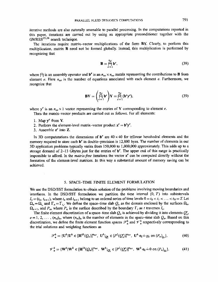
The plate has unit length and the origin of the co-ordinate system is attached to the leading edge. The rectangular computational domain, which spans the area defined by -0.1 6 x1 6 1.0 and 0.0 < x2 < 0.6, is discretized using 24,240 bilinear quadrilateral elements and 24,563 nodes. Figure 1 shows the finite element mesh used in this computation. This mesh is designed in such way that in the direction normal to the wall the minimum element length is 0.0012.

PARALLEL FLUID DYNAMICS COMPUTATIONS 793

Figure 1. Supersonic flow past a flat plate: finite element mesh

At the left and upper boundaries we impose Dirichlet-type boundary conditions for all primitive variables, density, velocity components and temperature. On the plate surface, zero velocity and heat flux are imposed. The symmetry boundary condition is used along the line connecting the plate tip to the left boundary. All boundary conditions at the outflow boundary are homogeneous Neumann-type.

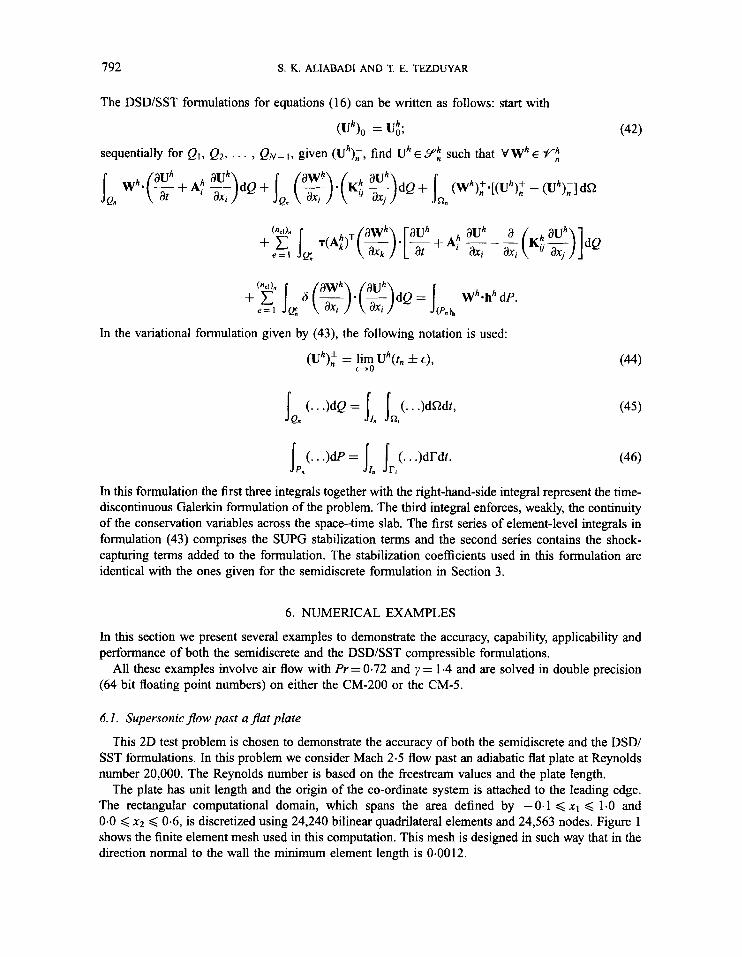
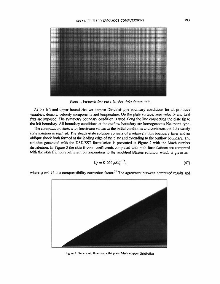
The computation starts with freestream values as the initial conditions and continues until the steady state solution is reached. The steady-state solution consists of a relatively thin boundary layer and an oblique shock both formed at the leading edge of the plate and extending to the outflow boundary. The solution generated with the DSDiSST formulation is presented in Figure 2 with the Mach number distribution. In Figure 3 the skin friction coefficients computed with both formulations are compared with the skin friction coefficient corresponding to the modified Blasius solution, which is given as

where + = 0-95 is a compressibility correction factor.27 The agreement between computed results and

Figure 2. Supersonic flow past a flat plate: Mach number distribution

794

0.18

0.16

S. K. ALIABADI AND T. E. TEZDUYAR

Semidiscrete formulation -.. . DSDISST formulation - '

.

0.06 p Semi-discrete formulation o

DSDISST formulation Modified Blasius

9

Figure 3. Supersonic flow past a flat plate: skin friction coefficient from computations and modified Blasius solution

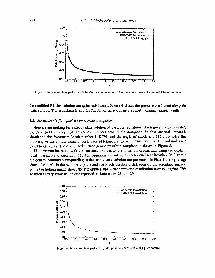
the modified Blasius solution are quite satisfactory. Figure 4 shows the pressure coefficient along the plate surface. The semidiscrete and DSD/SST formulations give almost indistinguishable results.

6.2. 3 0 tmnsonicJlow past a commercial aeroplane

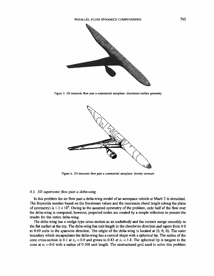
Here we are looking for a steady state solution of the Euler equations which govern approximately the flow field at very high Reynolds numbers around the aeroplane. In this inviscid, transonic simulation the freestream Mach number is 0.798 and the angle of attack is 1.116". To solve this problem, we use a finite element mesh made of tetrahedral element. This mesh has 106,064 nodes and 575,986 elements. The discretized surface geometry of the aeroplane is shown in Figure 5 .

The computation starts with the freestream values as the initial conditions and, using the explicit, local time-stepping algorithm, 513,365 equations are solved at each non-linear iteration. In Figure 6 the density contours corresponding to the steady state solution are presented. In Plate 1 the top image shows the mesh in the symmetry plane and the Mach number distribution on the aeroplane surface, while the bottom image shows the streamlines and surface pressure distribution near the engine. This solution is very close to the one reported in References 28 and 29.

0.14 8 0.12

l 0.06

8 0.10

0.08

0.04

0.02

o'?!O 0:l 0:2 0:3 0:4 0:s 0:6 0:7 0:s d9 X

Figure 4. Supersonic flow past a flat plate: pressure coefficient along plate surface

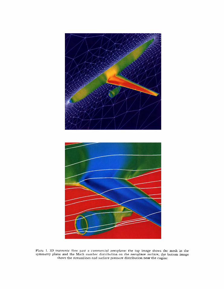
Plate 1. 3D transonic flow past a commercial aeroplane: the top image shows the mesh in the symmetry plane and the Mach number distribution on the aeroplane surface; the bottom image

shows the streamlines and surface pressure distribution near the engine

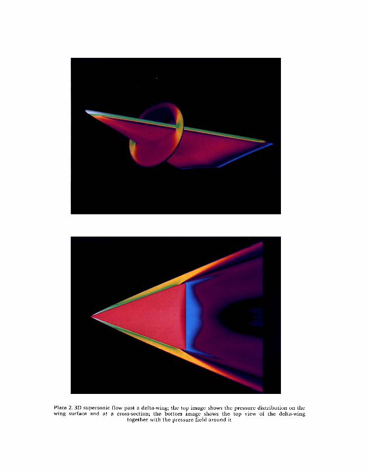
Plate 2. 3D supersonic flow past a delta-wing; the top image shows the pressure distribution on the wing surface and at a cross-section; the bottom image shows the top view of the delta-wing

together with the pressure field around it

Plate 3. 3D subsonic flow past a sphere: pressure distribution on sphere surface together with stream ribbons at time t = 200

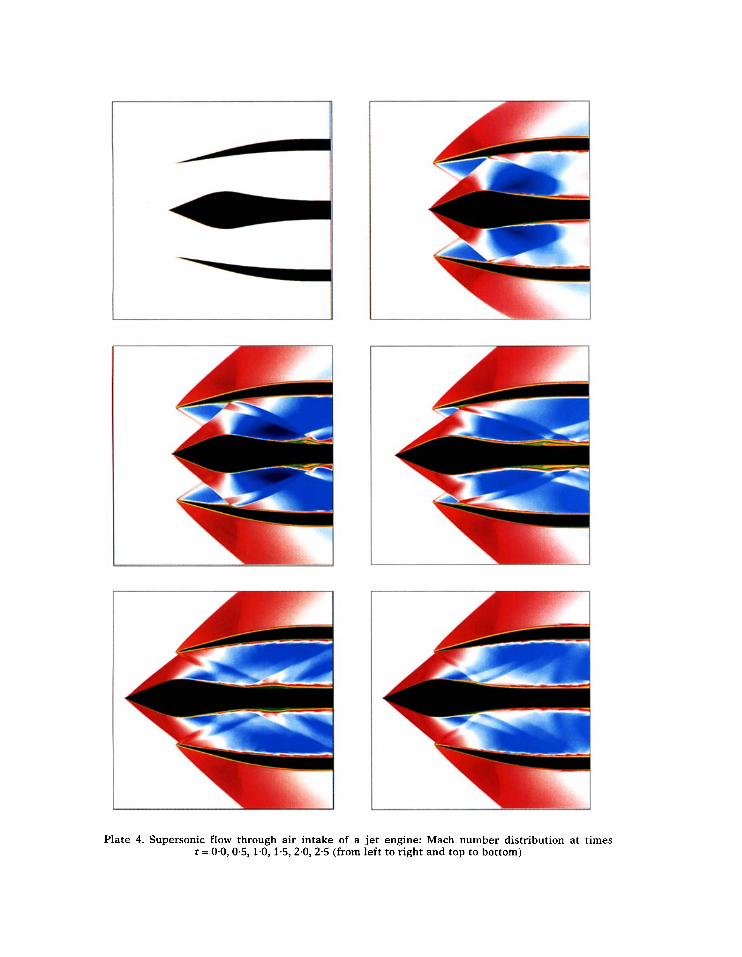
Plate 4. Supersonic flow through air intake of a jet engine: Mach number distribution at times t = 0.0,0.5,1.0,1.5,2.0,2.5 (from left to right and top to bottom)

PARALLEL FLUID DYNAMICS COMPUTATIONS

Figure 5. 3D transonic flow past a commercial aeroplane: discretized surface geometry

795

Figure 6. 3D transonic flow past a commercial aeroplane: density contours

6.3. 3 0 supersonic flow past a delta-wing

In this problem the air flow past a delta-wing model of an aerospace vehicle at Mach 3 is simulated. The Reynolds number based on the freestream values and the maximum chord length (along the plane of symmetry) is 1.1 x 1 06. Owing to the assumed symmetry of the problem, only half of the flow over the delta-wing is computed; however, projected nodes are created by a simple reflection to present the results for the entire delta-wing.

The delta-wing has a wedge-type cross-section as an underbody and the comers merge smoothly to the flat surfact at the top. The delta-wing has unit length in the chordwise direction and tapers from 0.0 to 0.69 units in the spanwise direction. The origin of the delta-wing is located at (0, 0, 0). The outer boundary which encapsulates the delta-wing has a conical shape with a spherical tip. The radius of the cone cross-section is 0.1 at x4 = 0-0 and grows to 0.83 at X I = 1-8. The spherical tip is tangent to the cone at x1 = 0.0 with a radius of 0.108 unit length. The unstructured grid used to solve this problem

796 S. K. ALIABADI AND T. E. TEZDUYAR

Figure 7. 3 iD supei rsonic flow past a delta wing: finite element mesh (coarsened for c :learer visualization)

consists of 1,032,328 nodes and 1,002,684 trilinear hexahedral elements. In order to capture the details of the boundary layer, the first three layers of elements are very close to the delta-wing surface. A significant portion of the mesh is placed in the wake region of the computational domain to model the flow in this region with considerable accuracy. A similar finite element mesh which has been coarsened for clearer visualization is partially shown in Figure 7.

The freestream values serve as the initial conditions and we stop the computations when the L2- norm of the residual is reduced by more than 2.5 orders of magnitude. At every time step 5,001,03 1 non-linear equations are solved simultaneously using matrix-free iterations.

Figures 8-10 show the Mach number contours corresponding to the steady state solution at three sections. In Plate 2 the top image shows the pressure distribution on the wing surface and a cross- section, while the bottom image shows the top view of the delta-wing together with the pressure field around it.

6.4. 3 0 subsonicjow past a sphere

Numerous experiments have been carried out to understand the structure of the wake of incompressible flow behind a sphere. At Reynolds numbers lower than about 350 the wake formed behind a sphere does not involve any instabilities and the flow is axisymmetric. The axisymmetric pattern of the flow breaks down at higher Reynolds numbers and the vortices begin to shed peri~dically.~' In the approximate range 350 d Re d 750 many researchers have reported one dominant mode of vortex shedding with the Strouhal number varying from 0.16 to 0.2, except for Reference 3 1 which reports another mode of vortex shedding. When the Reynolds number increases further, the flow becomes turbulent. In the approximate range 750 d Re < 10,000 two modes of vortex shedding exist. In one of the earliest experiments done by Mo11e?2 a high mode of vortex shedding was obtained with water. Later reported both low and high modes of vortex shedding behind a sphere at higher Reynolds numbers up to Re = lo5. Kim and D ~ r b i n ~ ~ associate the two modes of vortex shedding with the small-scale instability of the separating shear layer and with the large-scale instability of the wake.

We first check the steady state solutions at low Reynolds numbers to assess the accuracy of the

PARALLEL FLUID DYNAMICS COMPUTATIONS 797

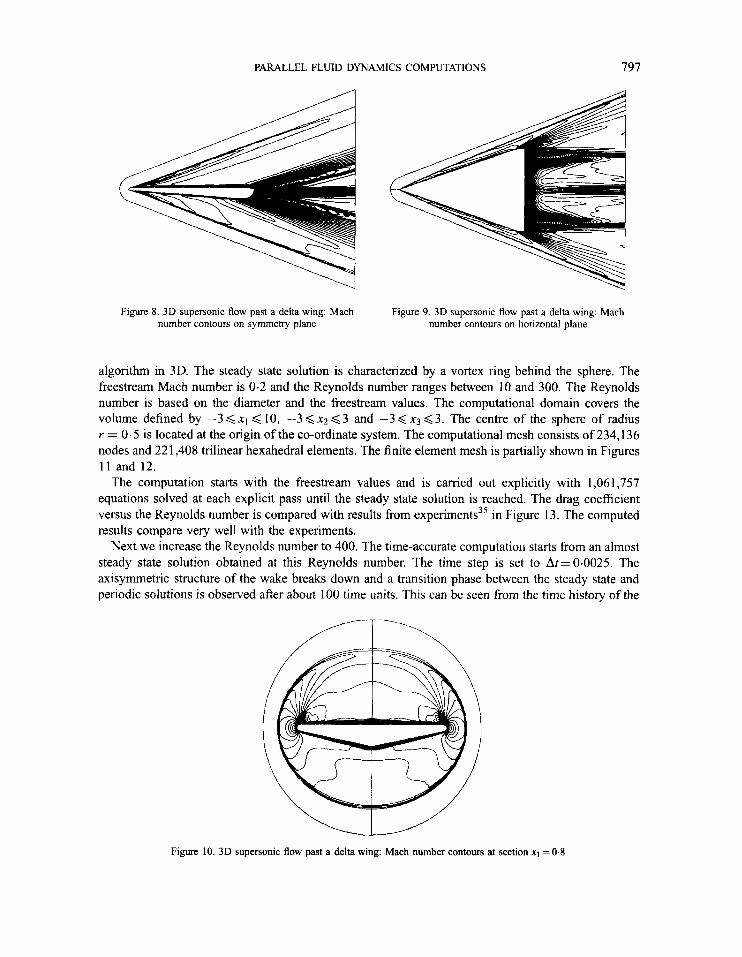
Figure 8. 3D supersonic flow past a delta wing: Mach number contours on symmetry plane

Figure 9. 3D supersonic flow past a delta wing: Mach number contours on horizontal plane

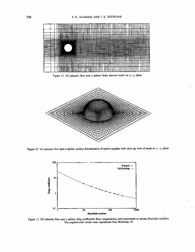
algorithm in 3D. The steady state solution is characterized by a vortex ring behind the sphere. The freestream Mach number is 0.2 and the Reynolds number ranges between 10 and 300. The Reynolds number is based on the diameter and the freestream values. The computational domain covers the volume defined by -3 <XI < 10, -3 < x2 < 3 and -3 < x3 < 3. The centre of the sphere of radius r = 0.5 is located at the origin of the co-ordinate system. The computational mesh consists of 234,136 nodes and 221,408 trilinear hexahedral elements. The finite element mesh is partially shown in Figures 11 and 12.

The computation starts with the freestream values and is camed out explicitly with 1,061,757 equations solved at each explicit pass until the steady state solution is reached. The drag coefficient versus the Reynolds number is compared with results from experiment^^^ in Figure 13. The computed results compare very well with the experiments.

Next we increase the Reynolds number to 400. The time-accurate computatiorl starts from an almost steady state solution obtained at this Reynolds number. The time step is set to At=0.0025. The axisymmetric structure of the wake breaks down and a transition phase between the steady state and periodic solutions is observed after about 100 time units. This can be seen from the time history of the

Figure 10. 3D supersonic flow past a delta wing: Mach number contours at section X I = 0.8

798

100 Resent o

Schlichting ----

---- -% ---. *- *.- -.. --a- s..

--*...- '-__ ---. " 10 7

8 .-

8

----. ---__ --__ -------- s-.- s" 1 -

0.1

S. K. ALIABADI AND T. E. TEZDUYAR

Figure 11. 3D subsonic flow past a sphere: finite element mexh on xI-xz plane

Figure 12. 3D subsonic flow past a sphere: surface discretization of sphere together with close-up view of mesh on xI-x2 plane

PARALLEL FLUID DYNAMICS COMPUTATIONS 799

drag coefficient in Figure 14. In the transition phase the vortex shedding appears in the symmetry plane. The time histories of the side force coefficients shown in Figure 15 illustrate the non-existence of plane symmetry when the flow is well established. The Strouhal number of vortex-shedding is 0.144. In experiments the Strouhal number is about 0-16 at Reynolds number 400. Plate 3 shows the pressure distribution on the sphere surface together with the stream ribbons at time t = 200.

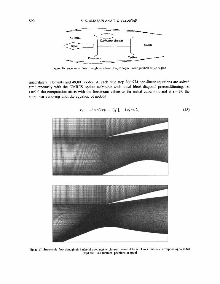
6.5. Supersonicflow through the air intake of a jet engine

This axisymmetric computation demonstrates the potential of the DSD/SST formulation to model intricate compressible flows involving interactions between boundary layers, shocks and moving surfaces. This type of flow is encountered in the air intake of a jet engine with adjustable spool (see Figure 16). The efficiency of these engines at supersonic speeds can be improved by moving the spool back and forth and thus adapting the outstanding shock. In this problem we consider internal and external flow passing an air intake. The freestream Mach number is 2 and the Reynolds number based on the freestream values and the gap size is 0.8 x 10'. The computational domain, which covers the area defined by - 0.25 -= x1 < 0.70 and 0.0 < x2 < 0.75, is discretized using 48,450 bilinear

0.66, I

- 0.63 4 0.62

0.50 0.59 IV I

40 80 120 160 200 240 280 320 0.57 A Time

Figure. 14. 3D subsonic flow past a sphere: time history of drag coefficient

Time Figure 15. 3D subsonic flow past a sphere: time histories of side force coefficients

800 S. K. ALIABADI AND T. E. TEZDUYAR

Compressor Turbine / - \

Figure 16. Supersonic flow through air intake of a jet engine: configuration of jet engine

quadrilateral elements and 49,091 nodes. At each time step 386,974 non-linear equations are solved simultaneously with the GMRES update technique with nodal block-diagonal preconditioning. At t= 0.0 the computation starts with the freestream values as the initial conditions and at t= 1.0 the spool starts moving with the equation of motion

x1 = -Lsin[2lr(t - l ) f ] , 1 6 1 6 2 ,

Figure 17. Supersonic flow through air intake of a jet engine: close-up views of finite element meshes corresponding to initial (top) and final (bottom) positions of spool

PARALLEL FLUID DYNAMICS COMPUTATIONS 80 1

where L = 0.2 is the maximum range of the motion and f = 0.25 is the frequency. For t > 2 the spool remains stationary.

The mesh-moving strategy used for this problem is such that the connectivity of the mesh remains unchanged throughout the simulation. This eliminates the projection errors associated with remeshing and also eliminates the parallelization overhead associated with remeshing . Figure 17 shows close-up views of the finite element meshes corresponding to the initial and final positions of the spool. A sequence of frames depicting the Mach number in the time interval [O-0, 2.51 is presented in Plate 4.

7. CONCLUSIONS

We select the delta-wing problem as a benchmark to measure the speed and efficiency of our computations on the Connection Machine CM-5. To investigate the scalability of the finite element programme, we employ three unstructured meshes with different levels of refinement to solve this problem. In all cases the numerical integration is achieved using 2 x 2 x 2 Gaussian quadrature and the non-linear system of equations is solved with the matrix-free GMRES iteration technique. The Krylov subspace dimension is set to 10.

Table I summarizes the performance of these computations on the CM-5. The reported computation rates exclude input and output (VO) tasks and the communication costs are measured compared with the total time again excluding I/O. From the results obtained, one can reach the following conclusions.

1. The scalability of the CM-5 system and the finite element solver is well established. The gigaFLOPS rates of 2 6 , 5.1 and 9.8, obtained on 128, 256 and 512 processing nodes respectively, all correspond to subgrid lengths (number of elements per processing node) in the range 195Ck2350. In other words, by keeping the subgrid length relatively high and almost constant, we obtain a linear speed-up as we increase the number of processors.

2. The communication cost decreases to a certain point as the subgrid size increases.

We also use the sphere problem to present the performance of our computations on different partitions of the CM-200. In this case the numerical integration is carried out using 2 x 2 x 2 Gaussian points and the solution of the non-linear system of equations is approximated with one explicit pass at

Table I. 3D supersonic flow past a delta-wing: implicit time integration performance on CM-5 with different partition sizes

Mesh 1 Mesh 2 Mesh 3 Nodes 309,507 Nodes 542,888 Nodes 1,032,328 Elements 297,624 Elements 523,674 Elements 1,002,684 Equations 1,495,112 Equations 2,628,126 Equations 5,001,031

Computation rate (gigaFLOPS)

Communication cost ("/I Non-linear iteration cost (shteration)

Non-linear iteration cost (pshteratiodnode)

128 PNs 256 PNs 512 PNs 128 PNs 256 PNs 512 PNs 128 PNs 256 PNs 512 PNs 128 PNs 256 PNs 512 PNs

2.6 5.6

11.6 12.6 23.2 27.0 16.7 7.7 3.7

54.5 24.9 11.9

- 5.1

12.4 -

13.5 18.5 -

14.7 6.0 -

27.1 11.1

- 14.5

802 S. K. ALIABADI AND T. E. TEZDUYAR

Table 11. 3D subsonic flow past a sphere: explicit time integration performance on CM-200 with different partition sizes

8192 16,384 32,768 processors processors processors

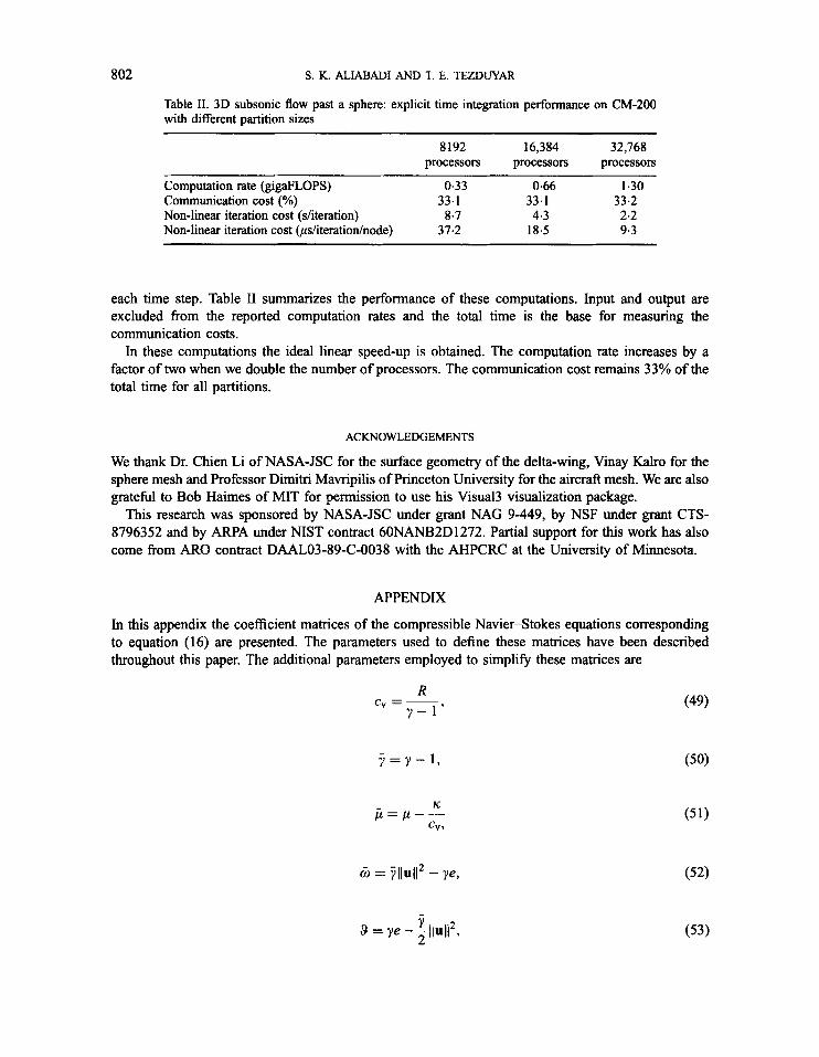
Computation rate (gigaFLOPS) 0.33 0.66 1.30 Communication cost (YO) 33.1 33.1 33.2 Non-linear iteration cost @/iteration) 8.7 4.3 2.2 Non-linear iteration cost (pliteratiodnode) 37.2 18.5 9.3

each time step. Table I1 summarizes the performance of these computations. Input and output are excluded from the reported computation rates and the total time is the base for measuring the communication costs.

In these computations the ideal linear speed-up is obtained. The computation rate increases by a factor of two when we double the number of processors. The communication cost remains 33% of the total time for all partitions.

ACKNOWLEDGEMENTS

We thank Dr. Chien Li of NASA-JSC for the surface geometry of the delta-wing, Vinay Kalro for the sphere mesh and Professor Dimitri Mavripilis of Princeton University for the aircraft mesh. We are also gratefid to Bob Haimes of MIT for permission to use his Visual3 visualization package.

This research was sponsored by NASA-JSC under grant NAG 9-449, by NSF under grant CTS- 8796352 and by ARPA under NIST contract 60NANB2D1272. Partial support for this work has also come from ARO contract DAALO3-89-C-0038 with the AHPCRC at the University of Minnesota.

APPENDIX

In this appendix the coefficient matrices of the compressible Navier-Stokes equations corresponding to equation (16) are presented. The parameters used to define these matrices have been described throughout this paper. The additional parameters employed to simplify these matrices are

R C" = ~

y - 1 ' (49)

PARALLEL FLUID DYNAMICS COMPUTATIONS

The coefficient matrices are then

1 K2l =-

P

803

(54)

804 S. K. ALIABADI AND T. E. TEZDUYAR

1 K22 == -

P

REFERENCES

1. T. J. R. Hughes and A. N. Brooks, ‘A multi-dimensional upwind scheme with no crosswind diffusion’, in T. J. R. Hughes (ed.) Finite Element Methods for Convection Dominated Flows, AMD Vol. 34, ASME, New York, 1979, pp. 19-35.

2. A. N. Brooks and T. J. R. Hughes. ‘Streamline upwind/Petrov-Galerkin formulations for convection dominated flows with particular emphasis on the incompressible Navier-Stokes equations’, Comput. Methods Appl. Mech. Eng., 32, 199-259 (1982).

3. T. E. Tezduyar and T. J. R. Hughes, ‘Finite element formulations for convection dominated flows with particular emphasis on the compressible Euler equations’, AIAA Paper 83-0125, 1983.

4. T. J. R. Hughes, L. P. Franca and M. Mallet, ‘A new finite element formulation for computational fluid dynamics: 1. Symmetric forms of the compressible Euler and Navier-Stokes equations and the second law of thermodynamics’, Comput. Methods Appl. Mech. Eng., 54, 223-234 (1986).

5. T. J. R. Hughes and M. Mallet, ‘A new finite element formulation for computational fluid dynamics: 111. The generalized streamline operator for multidimensional advective-diffisive systems’, Comput. Methods Appl. Mech. Eng. 58, 305-328 (1986).

6. T. J. R. Hughes and M. Mallet, ‘A new finite element formulation for computational fluid dynamics: I\! A discontinuity- capturing operator for multidimensional advective-diffisive systems’, Comput. Methods Appl. Mech. Eng., 58, 329-339 (1986).

7. G. J. Le Beau and T. E. Tezduyar, ‘Finite element computation of compressible flows with the SUPG formulation’, in M. N. Dhaubhadel, M. S. Engelman and J. N. Reddy (eds.), Advances in Finite Element Analysis in Fluid Dynamics, FED Vol. 123, ASME, New York, 1991, pp. 21-27.

8. G. J. Le Beau, S. E. Ray, S. K. Aliabadi and T. E. Tezduyar, ‘SUPG finite element computation of compressible flows with the entropy and conservation variables formulations’, Comput. Methodr Appl. Mech. Eng., 104, 2 7 4 2 (1993).

PARALLEL FLUID DYNAMICS COMPUTATIONS 805

9. S. K: Aliabadi, S. E. Ray and T. E. Tezduyar, ‘SUPG finite element computation of compressible flows with the entropy and conservation variables formulations’, Comput. Mech., 11, 300-3 12 (1 993).

10. S. K. Aliabadi and T. E. Tezduyar, ’Massively parallel compressible flow computations in aerospace applications’, Pre-conf: Proc. Second Japan-US Symp. on Finite Element Methods in Large-Scale Computational Fluid Dynamics, Tokyo, 1994.

11, T. Tezduyar, S. Aliabadi, M. Behr, A. Johnson and S. Mittal, ‘Massively parallel finite element computation of three- dimensional flow problems’, Proc. 6th Jn. Numerical Fluid Dynamics Symp., Tokyo, 1992, pp. 15-24.

12. T. Tezduyar, S. Aliabadi, M. Behr, A. Johnson and S. Mittal, ‘Parallel finite-element computation of 3D flows’, IEEE Comput., 26, (lo), 27-36 (1993).

13. C. W. Hirt, A. A. Amsden and J. L. Cook, ‘An arbitrary Lagrangian Eulerian computing method for all flow speeds’, l Comput. Phys., 14, 227-253 (1974).

14. T. J. R. Hughes, W. K. Liu and T. K. Zimmermann, ‘Lagangian-Eulerian finite element formulation for incompressible viscous flows’, Comput. Methods Appl. Mech. Eng., 29, 329-349 (1981).

15. B. Ramaswamy and M. Kawahara, ‘Arbitrary Lagrangian-Eulerian finite element method for unsteady, convective, incompressible viscous free surface fluid flow’, Int. j . numet methodspuids, 7 , 1053-1075 (1987).

16. A. Huerta and W. K. Liu, ‘Viscous flow with large free surface motion’, Comput. Methods Appl. Mech. Eng., 69, 277-324 (1988).

17. T. E. Tezduyar, M. Behr and J. Liou, ‘A new strategy for finite element computations involving moving boundaries and interfaces-the deforming-spatial-domaidspace-time procedure: 1. The concept and the preliminary tests’, Comput. Methods Appl. Mech. Eng., 94, 339-351 (1992).

18. T. E. Tezduyar, M. Behr, S. Mittal and J. Liou, ‘A new strategy for finite element compuations involving moving boundaries and interfaces-the deforming-spatial-domaidspacetime procedure: 11. Computation of free-surface flows, two-liquid flows, and flows with drifting cylinders’, Comput. Methods Appl. Mech. Eng., 94, 353-371 (1992).

19. S. K. Aliabadi and T. E. Tezduyar, ‘Space-time finite element computation of compressible flows involving moving boundaries and interfaces’, Comput. Methods Appl. Mech. Eng., 107, 209-224 (1993).

20. M. Mallet, ‘A finite element method for computational fluid dynamics’, Ph.D. Thesis, Department of Civil Engineering, Stanford University, 1985.

21. T. E. Tezduyar and T. J. R. Hughes, ‘Development of time-accurate finite element techniques for first-order hyperbolic systems with particular emphasis on the compressible Euler equations’, NASA-Ames University Consortium Interchange, Rep. NCA2-OR745-I 04, 1982.

22. F. Shakib, ‘Finite element analysis o f the compressible Euler and Navier-Stokes equations’, Ph.D. Thesis, Department of Mechanical Engineering, Stanford University, 1988.

23. T. J. R. Hughes, The Finite Element Method, Linear Static and Dynamic Finite Element Analysis, Prentice-Hall, Engelwood Cliffs, NJ, 1987.

24. M. Behr, ‘Stabilized finite element methods for incompressible flows with emphasis on moving boundaries and interfaces’, Ph.D. Thesis, Department of Aerospace Engineering, University of Minnesota, 1992.

25. Y. Saad and M. Schultz, ‘GMRES: a generalized minimal residual algorithm for solving nonsymmetric linear systems’, SIAMl Sci. Stat. Comput., 7, 856-869 (1986).

26. Y. Saad, ‘A flexible inner-outer preconditioned GMRES algorithm’, SIAMl Sci. Comput. 14, 461469 (1993). 27. J. Cousteix, Turbulence et Couche Limife, Cepadues Editions, 1990. 28. R. Das, D. J. Mavriplis, J. Saltz, S. Gupta and R. Ponnusamy, ‘The design and implementaiton of parallel unstructured Euler

29. Z. Johan, K. K. Mathur and S. L. Johnsson, ‘An efficient communication strategy for finite element methods on the

30. H. Sakamotto and H. Haniu, ‘A study on vortex shedding from spheres in a uniform flow’, JT Fluids Eng., 112, 386-392

31. R. H. Magarvey and R. L. Bishop, ‘Wakes in liquid-liquid systems’, Phys. Fluids, 4, 800-805 (1961). 32. W. Moller, ‘Experimentelle Untersuchung zur Hydromechanick der Hugel’, Phys. Z., 35, 57-80 (1938). 33. C. Cometta, ‘An investigation o f the unsteady flow pattern in the wake of cylinder and spheres using a hot wire probe’, Tech.

34. K. J. Kim and P A. Durbin, ‘Observation of the frequencies in a sphere wake and drag increase by acoustic excitation’, Phys.

35. H. Schlichting, Boundary-Layer Theory, 7th edn., McGraw-Hill, New York, 1979.

solver using software primitives’, .4IAA Paper 92-0562, 1992.

connection machine CM-5’, Comput. Methods Appl. Mech. Eng., in press.

(1990).

Rep. WT-21, Division of Engineering, Brown University, 1957.

Fluids, 31, 3260-3265 (1961).