parallel cellular automata: a model program for ...oberon2005.oberoncore.ru/classics/bh1993b.pdf ·...
TRANSCRIPT
Parallel Cellular Automata: A ModelProgram for Computational Science∗
(1993)
We develop a generic program for parallel execution of cellular automata on
a multicomputer. The generic program is then adapted for simulation of a
forest fire and numerical solution of Laplace’s equation for stationary heat
flow. The performance of the parallel program is analyzed and measured on
a Computing Surface configured as a matrix of transputers with distributed
memory.
1 Introduction
This is one of several papers that explore the benefits of developing modelprograms for computational science (Brinch Hansen 1990, 1991a, 1991b,1992a). The theme of this paper is parallel cellular automata.
A cellular automaton is a discrete model of a system that varies in spaceand time. The discrete space is an array of identical cells, each representing alocal state. As time advances in discrete steps, the system evolves accordingto universal laws. Every time the clock ticks, the cells update their statessimultaneously. The next state of a cell depends only on the current stateof the cell and its nearest neighbors.
In 1950 John von Neuman and Stan Ulam introduced cellular automatato study self-reproducing systems (von Neumann 1966; Ulam 1986). JohnConway’s game of Life is undoubtedly the most widely known cellular au-tomaton (Gardner 1970, 1971; Berlekamp 1982). Another well known au-tomaton simulates the life cycles of sharks and fish on the imaginary planet
∗P. Brinch Hansen, Parallel Cellular Automata: A model program for computationalscience. Concurrency—Practice and Experience 5, 5 (August 1993), 425–448. Copyrightc© 1993, John Wiley & Sons, Ltd. Revised version.
1
2 PER BRINCH HANSEN
Wa-Tor (Dewdney 1984). The numerous applications include forest infesta-tion (Hoppensteadt 1978), fluid flow (Frisch 1986), earthquakes (Bak 1989),forest fires (Bak 1990) and sandpile avalanches (Hwa 1989).
Cellular automata can simulate continuous physical systems described bypartial differential equations. The numerical solution of, say, Laplace’s equa-tion by grid relaxation is really a discrete simulation of heat flow performedby a cellular automaton.
Cellular automata are ideally suited for parallel computing. My goalis to explore programming methodology for multicomputers. I will illustratethis theme by developing a generic program for parallel execution of cellularautomata on a multicomputer with a square matrix of processor nodes. Iwill then show how easy it is to adapt the generic program for two differentapplications: (1) simulation of a forest fire, and (2) numerical solution ofLaplace’s equation for stationary heat flow. On a Computing Surface withtransputer nodes, the parallel efficiency of these model programs is close toone.
2 Cellular Automata
A cellular automaton is an array of parallel processes, known as cells. Everycell has a discrete state. At discrete moments in time, the cells update theirstates simultaneously. The state transition of a cell depends only on itsprevious state and the states of the adjacent cells.
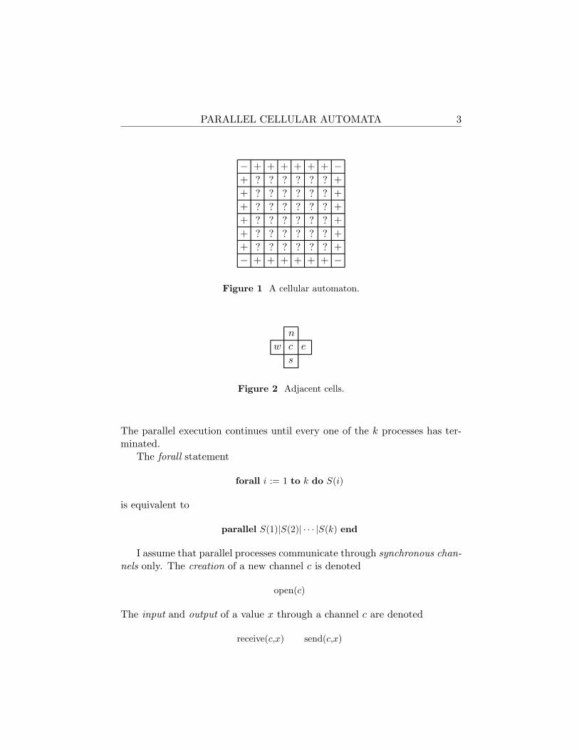
I will program a two-dimensional cellular automaton with fixed boundarystates (Fig. 1). The automaton is a square matrix with three kinds of cells:
1. Interior cells, marked “?”, may change their states dynamically.
2. Boundary cells, marked “+”, have fixed states.
3. Corner cells, marked“−”, are not used.
Figure 2 shows an interior cell and the four neighbors that may influenceits state. These five cells are labeled c (central), n (north), s (south), e (east),and w (west).
The cellular automaton will be programmed in SuperPascal (Brinch Han-sen 1994). The execution of k statements S1, S2, . . . , Sk as parallel processesis denoted
parallel S1|S2| · · · |Sk end
PARALLEL CELLULAR AUTOMATA 3
− −+ + + + + +
− −+ + + + + +++++++
??????
??????
??????
??????
??????
??????
++++++
Figure 1 A cellular automaton.
n
w c e
s
Figure 2 Adjacent cells.
The parallel execution continues until every one of the k processes has ter-minated.
The forall statement
forall i := 1 to k do S(i)
is equivalent to
parallel S(1)|S(2)| · · · |S(k) end
I assume that parallel processes communicate through synchronous chan-nels only. The creation of a new channel c is denoted
open(c)
The input and output of a value x through a channel c are denoted
receive(c,x) send(c,x)
4 PER BRINCH HANSEN
A cellular automaton is a set of parallel communicating cells. If you ig-nore boundary cells and communication details, a two-dimensional automa-ton is defined as follows:
forall i := 1 to n doforall j := 1 to n do
cell(i,j)
After initializing its own state, every interior cell goes through a fixednumber of state transitions before outputting its final state:
initialize own state;for k := 1 to steps do
beginexchange states with
adjacent cells;update own state
end;output own state
The challenge is to transform this fine-grained parallel model into anefficient program for a multicomputer with distributed memory.
3 Initial States
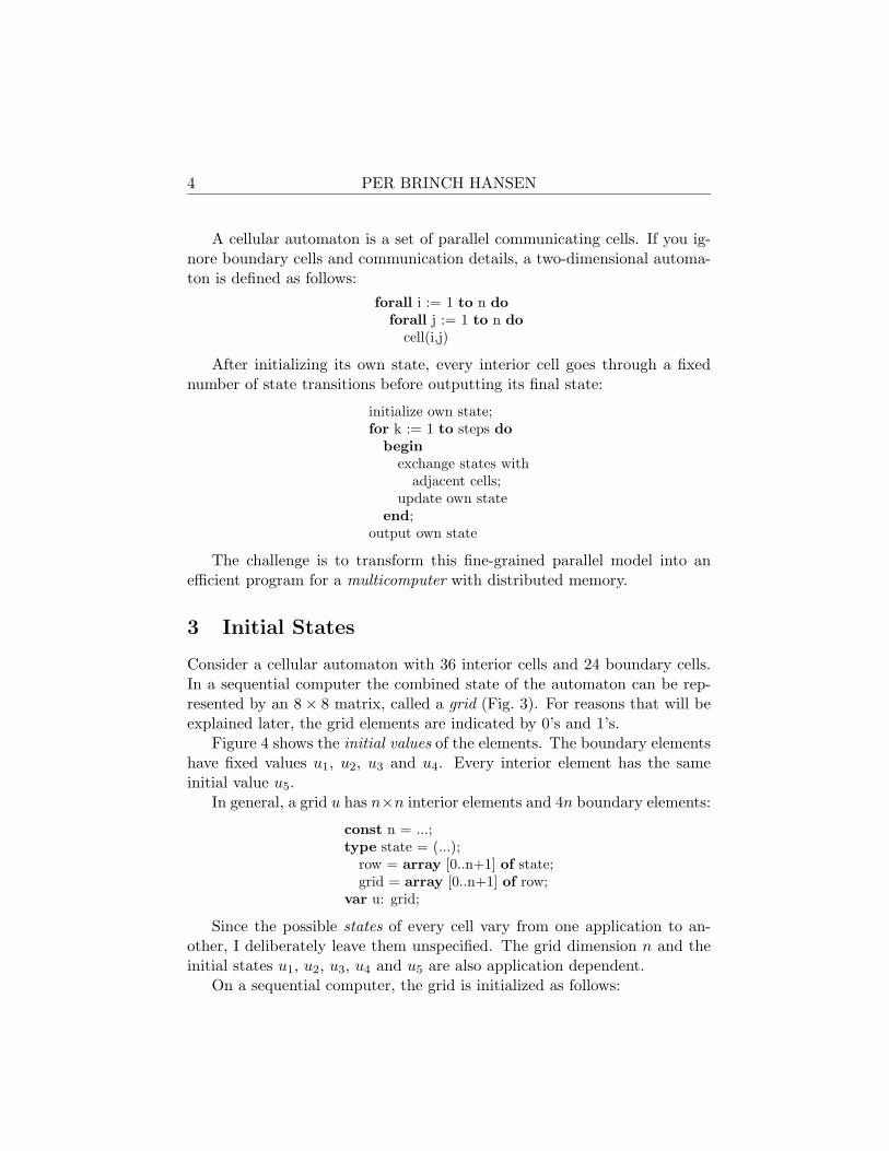
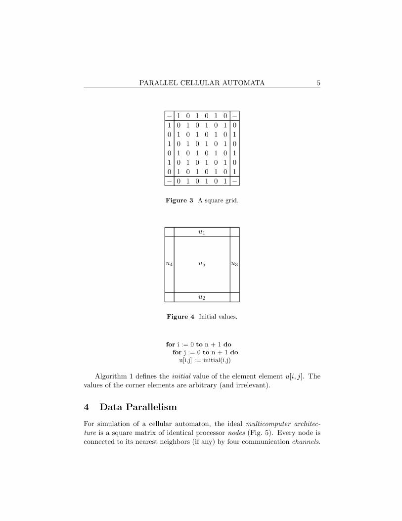
Consider a cellular automaton with 36 interior cells and 24 boundary cells.In a sequential computer the combined state of the automaton can be rep-resented by an 8× 8 matrix, called a grid (Fig. 3). For reasons that will beexplained later, the grid elements are indicated by 0’s and 1’s.
Figure 4 shows the initial values of the elements. The boundary elementshave fixed values u1, u2, u3 and u4. Every interior element has the sameinitial value u5.
In general, a grid u has n×n interior elements and 4n boundary elements:
const n = ...;type state = (...);
row = array [0..n+1] of state;grid = array [0..n+1] of row;
var u: grid;
Since the possible states of every cell vary from one application to an-other, I deliberately leave them unspecified. The grid dimension n and theinitial states u1, u2, u3, u4 and u5 are also application dependent.
On a sequential computer, the grid is initialized as follows:
PARALLEL CELLULAR AUTOMATA 5
− −1 1 10 0 01 1 1 10 0 0 00 0 0 01 1 1 11 1 1 10 0 0 00 0 0 01 1 1 11 1 1 10 0 0 00 0 0 01 1 1 1− −0 0 01 1 1
Figure 3 A square grid.
u1
u2
u3u4 u5
Figure 4 Initial values.
for i := 0 to n + 1 dofor j := 0 to n + 1 do
u[i,j] := initial(i,j)
Algorithm 1 defines the initial value of the element element u[i, j]. Thevalues of the corner elements are arbitrary (and irrelevant).
4 Data Parallelism
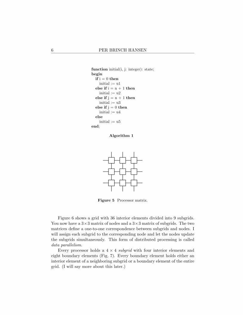
For simulation of a cellular automaton, the ideal multicomputer architec-ture is a square matrix of identical processor nodes (Fig. 5). Every node isconnected to its nearest neighbors (if any) by four communication channels.
6 PER BRINCH HANSEN
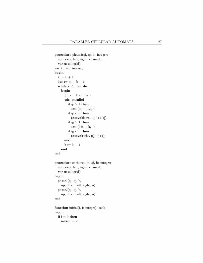
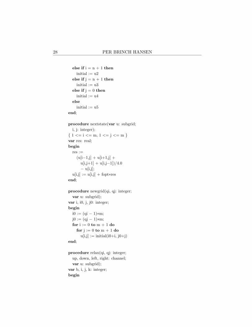
function initial(i, j: integer): state;begin
if i = 0 theninitial := u1
else if i = n + 1 theninitial := u2
else if j = n + 1 theninitial := u3
else if j = 0 theninitial := u4
elseinitial := u5
end;
Algorithm 1
Figure 5 Processor matrix.
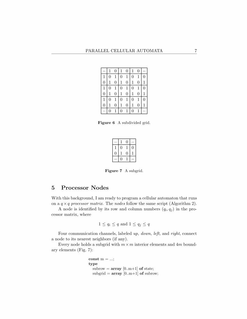
Figure 6 shows a grid with 36 interior elements divided into 9 subgrids.You now have a 3×3 matrix of nodes and a 3×3 matrix of subgrids. The twomatrices define a one-to-one correspondence between subgrids and nodes. Iwill assign each subgrid to the corresponding node and let the nodes updatethe subgrids simultaneously. This form of distributed processing is calleddata parallelism.
Every processor holds a 4 × 4 subgrid with four interior elements andeight boundary elements (Fig. 7). Every boundary element holds either aninterior element of a neighboring subgrid or a boundary element of the entiregrid. (I will say more about this later.)
PARALLEL CELLULAR AUTOMATA 7
− −1 1 10 0 01 1 1 10 0 0 00 0 0 01 1 1 11 1 1 10 0 0 00 0 0 01 1 1 11 1 1 10 0 0 00 0 0 01 1 1 1− −0 0 01 1 1
Figure 6 A subdivided grid.
− −1 01 10 00 01 1− −0 1
Figure 7 A subgrid.
5 Processor Nodes
With this background, I am ready to program a cellular automaton that runson a q×q processor matrix. The nodes follow the same script (Algorithm 2).
A node is identified by its row and column numbers (qi, qj) in the pro-cessor matrix, where
1 ≤ qi ≤ q and 1 ≤ qj ≤ q
Four communication channels, labeled up, down, left, and right, connecta node to its nearest neighbors (if any).
Every node holds a subgrid with m×m interior elements and 4m bound-ary elements (Fig. 7):
const m = ...;type
subrow = array [0..m+1] of state;subgrid = array [0..m+1] of subrow;
8 PER BRINCH HANSEN
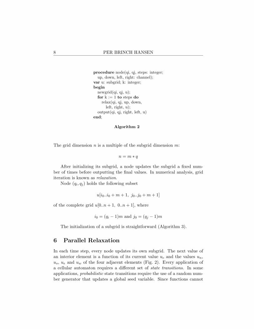
procedure node(qi, qj, steps: integer;up, down, left, right: channel);
var u: subgrid; k: integer;begin
newgrid(qi, qj, u);for k := 1 to steps do
relax(qi, qj, up, down,left, right, u);
output(qi, qj, right, left, u)end;
Algorithm 2
The grid dimension n is a multiple of the subgrid dimension m:
n = m ∗ q
After initializing its subgrid, a node updates the subgrid a fixed num-ber of times before outputting the final values. In numerical analysis, griditeration is known as relaxation.
Node (qi, qj) holds the following subset
u[i0..i0 +m+ 1, j0..j0 +m+ 1]
of the complete grid u[0..n+ 1, 0..n+ 1], where
i0 = (qi − 1)m and j0 = (qj − 1)m
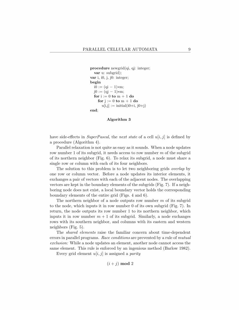
The initialization of a subgrid is straightforward (Algorithm 3).
6 Parallel Relaxation
In each time step, every node updates its own subgrid. The next value ofan interior element is a function of its current value uc and the values un,us, ue and uw of the four adjacent elements (Fig. 2). Every application ofa cellular automaton requires a different set of state transitions. In someapplications, probabilistic state transitions require the use of a random num-ber generator that updates a global seed variable. Since functions cannot
PARALLEL CELLULAR AUTOMATA 9
procedure newgrid(qi, qj: integer;var u: subgrid);
var i, i0, j, j0: integer;begin
i0 := (qi − 1)∗m;j0 := (qj − 1)∗m;for i := 0 to m + 1 do
for j := 0 to m + 1 dou[i,j] := initial(i0+i, j0+j)
end;
Algorithm 3
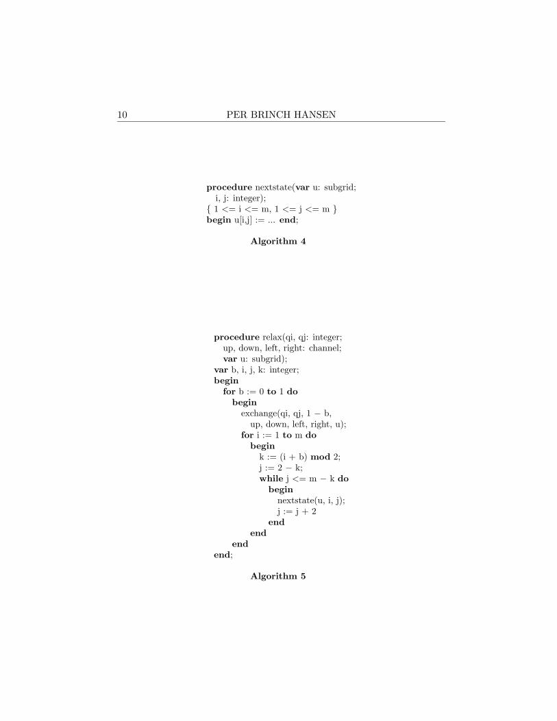
have side-effects in SuperPascal, the next state of a cell u[i, j] is defined bya procedure (Algorithm 4).
Parallel relaxation is not quite as easy as it sounds. When a node updatesrow number 1 of its subgrid, it needs access to row number m of the subgridof its northern neighbor (Fig. 6). To relax its subgrid, a node must share asingle row or column with each of its four neighbors.
The solution to this problem is to let two neighboring grids overlap byone row or column vector. Before a node updates its interior elements, itexchanges a pair of vectors with each of the adjacent nodes. The overlappingvectors are kept in the boundary elements of the subgrids (Fig. 7). If a neigh-boring node does not exist, a local boundary vector holds the correspondingboundary elements of the entire grid (Figs. 4 and 6).
The northern neighbor of a node outputs row number m of its subgridto the node, which inputs it in row number 0 of its own subgrid (Fig. 7). Inreturn, the node outputs its row number 1 to its northern neighbor, whichinputs it in row number m + 1 of its subgrid. Similarly, a node exchangesrows with its southern neighbor, and columns with its eastern and westernneighbors (Fig. 5).
The shared elements raise the familiar concern about time-dependenterrors in parallel programs. Race conditions are prevented by a rule of mutualexclusion: While a node updates an element, another node cannot access thesame element. This rule is enforced by an ingenious method (Barlow 1982).
Every grid element u[i, j] is assigned a parity
(i+ j) mod 2
10 PER BRINCH HANSEN
procedure nextstate(var u: subgrid;i, j: integer);{ 1 <= i <= m, 1 <= j <= m }begin u[i,j] := ... end;
Algorithm 4
procedure relax(qi, qj: integer;up, down, left, right: channel;var u: subgrid);
var b, i, j, k: integer;begin
for b := 0 to 1 dobegin
exchange(qi, qj, 1 − b,up, down, left, right, u);
for i := 1 to m dobegin
k := (i + b) mod 2;j := 2 − k;while j <= m − k do
beginnextstate(u, i, j);j := j + 2
endend
endend;
Algorithm 5

PARALLEL CELLULAR AUTOMATA 11
which is either even (0) or odd (1) as shown in Figs. 3 and 6. To eliminatetedious (and unnecessary) programming details, I assume that the subgriddimension m is even. This guarantees that every subgrid has the same parityordering of the elements (Figs. 6 and 7).
Parity ordering reveals a simple property of grids: The next values ofthe even interior elements depend only on the current values of the oddelements, and vice versa. This observation suggests a reliable method forparallel relaxation.
In each relaxation step, the nodes scan their grids twice:
• First scan: The nodes exchange odd elements with their neighbors andupdate all even interior elements simultaneously.
• Second scan: The nodes exchange even elements and update all oddinterior elements simultaneously.
The key point is this: In each scan, the simultaneous updating of localelements depends only on shared elements with constant values! In theterminology of parallel programming, the nodes are disjoint processes duringa scan.
The relaxation procedure uses a local variable to update elements withthe same parity b after exchanging elements of the opposite parity 1− b withits neighbors (Algorithm 5).
7 Local Communication
The nodes communicate through synchronous channels with the followingproperties:
1. Every channel connects exactly two nodes.
2. The communications on a channel take place one at a time.
3. A communication takes place when a node is ready to output a valuethrough a channel and another node is ready to input the value throughthe same channel.
4. A channel can transmit a value in either direction between two nodes.
5. The four channels of a node can transmit values simultaneously.
12 PER BRINCH HANSEN
These requirements are satisfied by transputer nodes programmed in occam(Cok 1991).
The identical behavior of the nodes poses a subtle problem. Suppose thenodes simultaneously attempt to input from their northern neighbors. Inthat case, the nodes will deadlock, since none of them are ready to outputthrough the corresponding channels. There are several solutions to thisproblem. I use a method that works well for transputers.
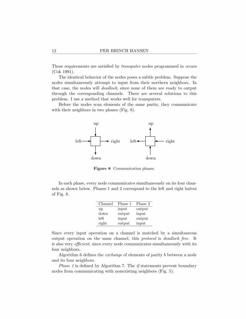
Before the nodes scan elements of the same parity, they communicatewith their neighbors in two phases (Fig. 8).
up up
down down
left leftright right?
?
- -
6
6
��
Figure 8 Communication phases.
In each phase, every node communicates simultaneously on its four chan-nels as shown below. Phases 1 and 2 correspond to the left and right halvesof Fig. 8.
Channel Phase 1 Phase 2up input outputdown output inputleft input outputright output input
Since every input operation on a channel is matched by a simultaneousoutput operation on the same channel, this protocol is deadlock free. Itis also very efficient, since every node communicates simultaneously with itsfour neighbors.
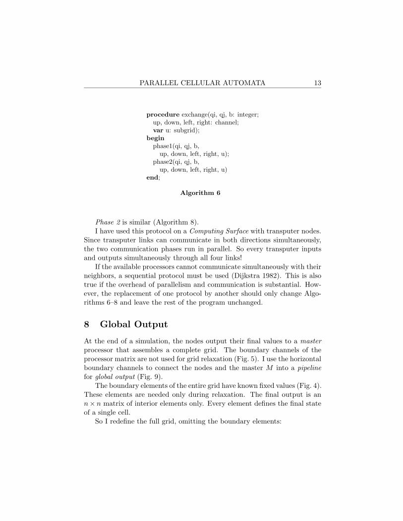
Algorithm 6 defines the exchange of elements of parity b between a nodeand its four neighbors.
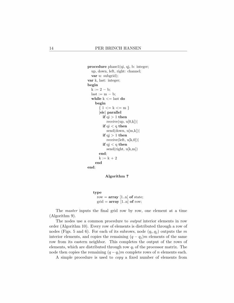
Phase 1 is defined by Algorithm 7. The if statements prevent boundarynodes from communicating with nonexisting neighbors (Fig. 5).
PARALLEL CELLULAR AUTOMATA 13
procedure exchange(qi, qj, b: integer;up, down, left, right: channel;var u: subgrid);
beginphase1(qi, qj, b,
up, down, left, right, u);phase2(qi, qj, b,
up, down, left, right, u)end;
Algorithm 6
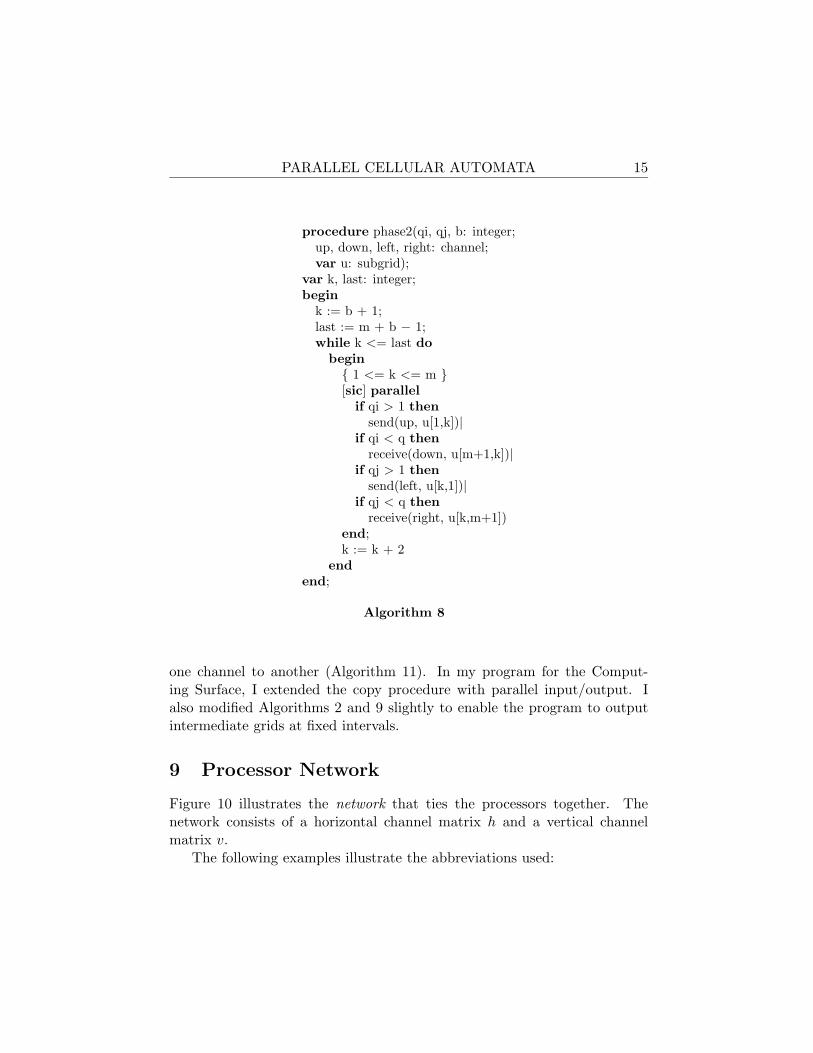
Phase 2 is similar (Algorithm 8).I have used this protocol on a Computing Surface with transputer nodes.
Since transputer links can communicate in both directions simultaneously,the two communication phases run in parallel. So every transputer inputsand outputs simultaneously through all four links!
If the available processors cannot communicate simultaneously with theirneighbors, a sequential protocol must be used (Dijkstra 1982). This is alsotrue if the overhead of parallelism and communication is substantial. How-ever, the replacement of one protocol by another should only change Algo-rithms 6–8 and leave the rest of the program unchanged.
8 Global Output
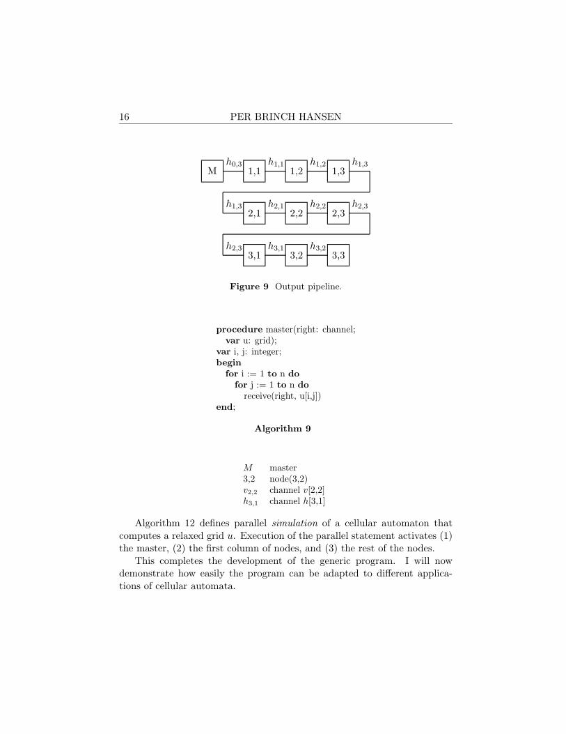
At the end of a simulation, the nodes output their final values to a masterprocessor that assembles a complete grid. The boundary channels of theprocessor matrix are not used for grid relaxation (Fig. 5). I use the horizontalboundary channels to connect the nodes and the master M into a pipelinefor global output (Fig. 9).
The boundary elements of the entire grid have known fixed values (Fig. 4).These elements are needed only during relaxation. The final output is ann× n matrix of interior elements only. Every element defines the final stateof a single cell.
So I redefine the full grid, omitting the boundary elements:
14 PER BRINCH HANSEN
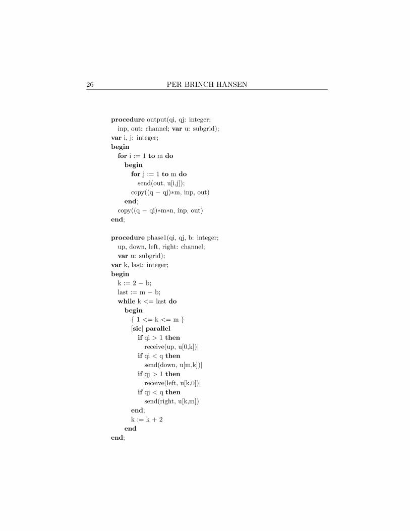
procedure phase1(qi, qj, b: integer;up, down, left, right: channel;var u: subgrid);
var k, last: integer;begin
k := 2 − b;last := m − b;while k <= last do
begin{ 1 <= k <= m }[sic] parallel
if qi > 1 thenreceive(up, u[0,k])|
if qi < q thensend(down, u[m,k])|
if qj > 1 thenreceive(left, u[k,0])|
if qj < q thensend(right, u[k,m])
end;k := k + 2
endend;
Algorithm 7
typerow = array [1..n] of state;grid = array [1..n] of row;
The master inputs the final grid row by row, one element at a time(Algorithm 9).
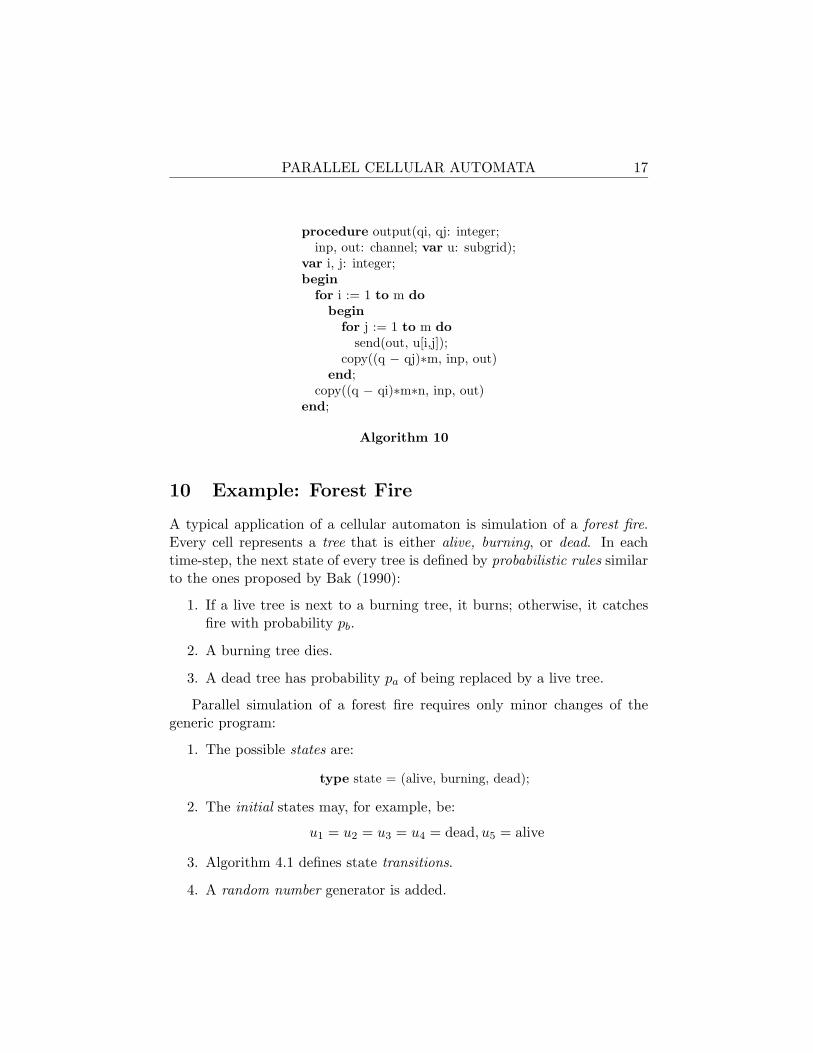
The nodes use a common procedure to output interior elements in roworder (Algorithm 10). Every row of elements is distributed through a row ofnodes (Figs. 5 and 6). For each of its subrows, node (qi, qj) outputs the minterior elements, and copies the remaining (q − qj)m elements of the samerow from its eastern neighbor. This completes the output of the rows ofelements, which are distributed through row qi of the processor matrix. Thenode then copies the remaining (q− qi)m complete rows of n elements each.
A simple procedure is used to copy a fixed number of elements from
PARALLEL CELLULAR AUTOMATA 15
procedure phase2(qi, qj, b: integer;up, down, left, right: channel;var u: subgrid);
var k, last: integer;begin
k := b + 1;last := m + b − 1;while k <= last do
begin{ 1 <= k <= m }[sic] parallel
if qi > 1 thensend(up, u[1,k])|
if qi < q thenreceive(down, u[m+1,k])|
if qj > 1 thensend(left, u[k,1])|
if qj < q thenreceive(right, u[k,m+1])
end;k := k + 2
endend;
Algorithm 8
one channel to another (Algorithm 11). In my program for the Comput-ing Surface, I extended the copy procedure with parallel input/output. Ialso modified Algorithms 2 and 9 slightly to enable the program to outputintermediate grids at fixed intervals.
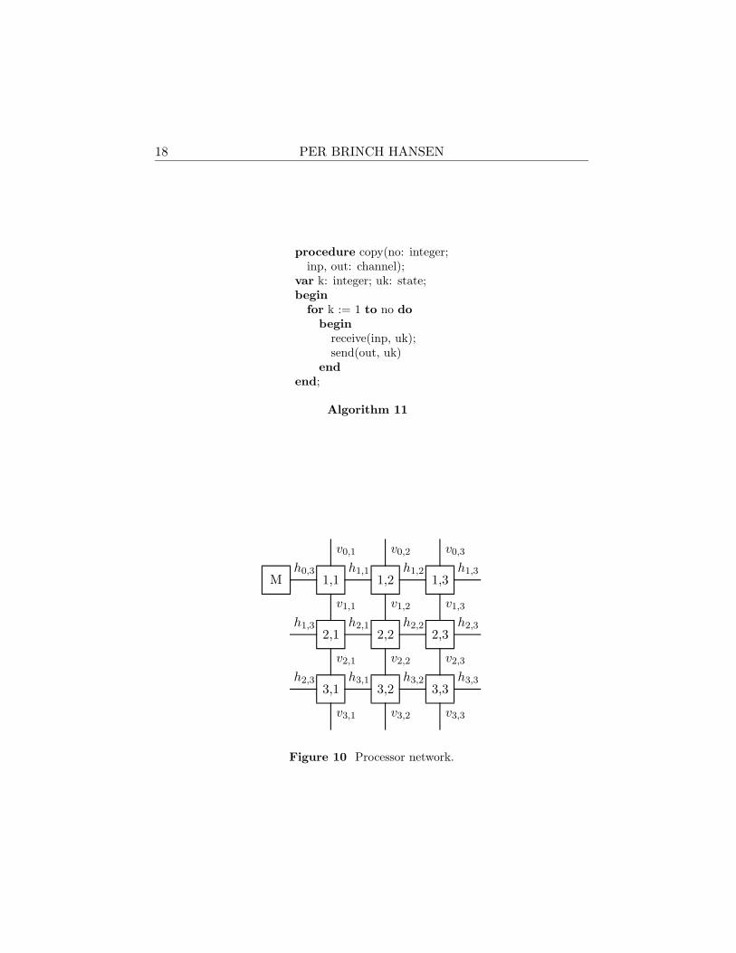
9 Processor Network
Figure 10 illustrates the network that ties the processors together. Thenetwork consists of a horizontal channel matrix h and a vertical channelmatrix v.
The following examples illustrate the abbreviations used:
16 PER BRINCH HANSEN
M 1,1 1,2 1,3
2,1 2,2 2,3
3,1 3,2 3,3
h0,3
h1,3
h2,3
h1,1
h2,1
h3,1
h1,2
h2,2
h3,2
h1,3
h2,3
Figure 9 Output pipeline.
procedure master(right: channel;var u: grid);
var i, j: integer;begin
for i := 1 to n dofor j := 1 to n do
receive(right, u[i,j])end;
Algorithm 9
M master3,2 node(3,2)v2,2 channel v[2,2]h3,1 channel h[3,1]
Algorithm 12 defines parallel simulation of a cellular automaton thatcomputes a relaxed grid u. Execution of the parallel statement activates (1)the master, (2) the first column of nodes, and (3) the rest of the nodes.
This completes the development of the generic program. I will nowdemonstrate how easily the program can be adapted to different applica-tions of cellular automata.
PARALLEL CELLULAR AUTOMATA 17
procedure output(qi, qj: integer;inp, out: channel; var u: subgrid);
var i, j: integer;begin
for i := 1 to m dobegin
for j := 1 to m dosend(out, u[i,j]);
copy((q − qj)∗m, inp, out)end;
copy((q − qi)∗m∗n, inp, out)end;
Algorithm 10
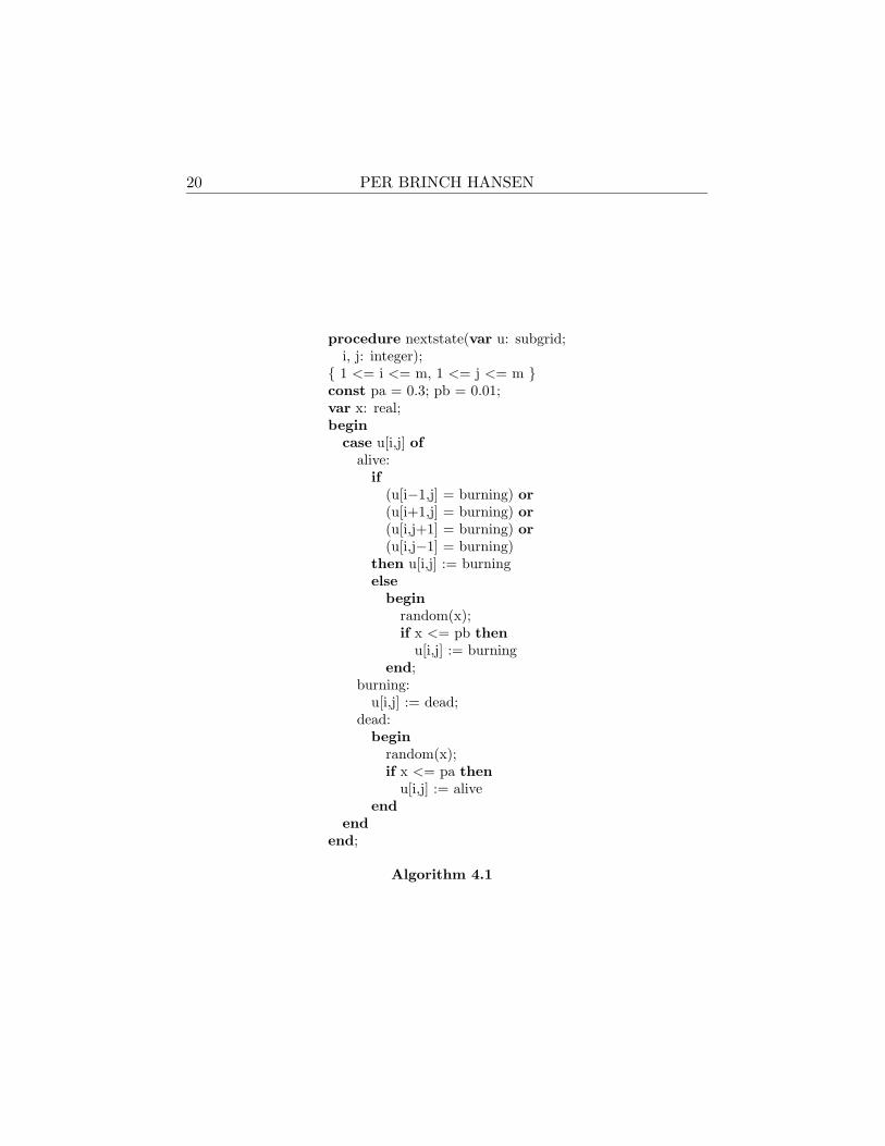
10 Example: Forest Fire
A typical application of a cellular automaton is simulation of a forest fire.Every cell represents a tree that is either alive, burning, or dead. In eachtime-step, the next state of every tree is defined by probabilistic rules similarto the ones proposed by Bak (1990):
1. If a live tree is next to a burning tree, it burns; otherwise, it catchesfire with probability pb.
2. A burning tree dies.
3. A dead tree has probability pa of being replaced by a live tree.
Parallel simulation of a forest fire requires only minor changes of thegeneric program:
1. The possible states are:
type state = (alive, burning, dead);
2. The initial states may, for example, be:
u1 = u2 = u3 = u4 = dead, u5 = alive
3. Algorithm 4.1 defines state transitions.
4. A random number generator is added.
18 PER BRINCH HANSEN
procedure copy(no: integer;inp, out: channel);
var k: integer; uk: state;begin
for k := 1 to no dobegin
receive(inp, uk);send(out, uk)
endend;
Algorithm 11
M 1,1 1,2 1,3
2,1 2,2 2,3
3,1 3,2 3,3
v0,1
v1,1
v2,1
v3,1
v0,2
v1,2
v2,2
v3,2
v0,3
v1,3
v2,3
v3,3
h0,3
h1,3
h2,3
h1,1
h2,1
h3,1
h1,2
h2,2
h3,2
h1,3
h2,3
h3,3
Figure 10 Processor network.
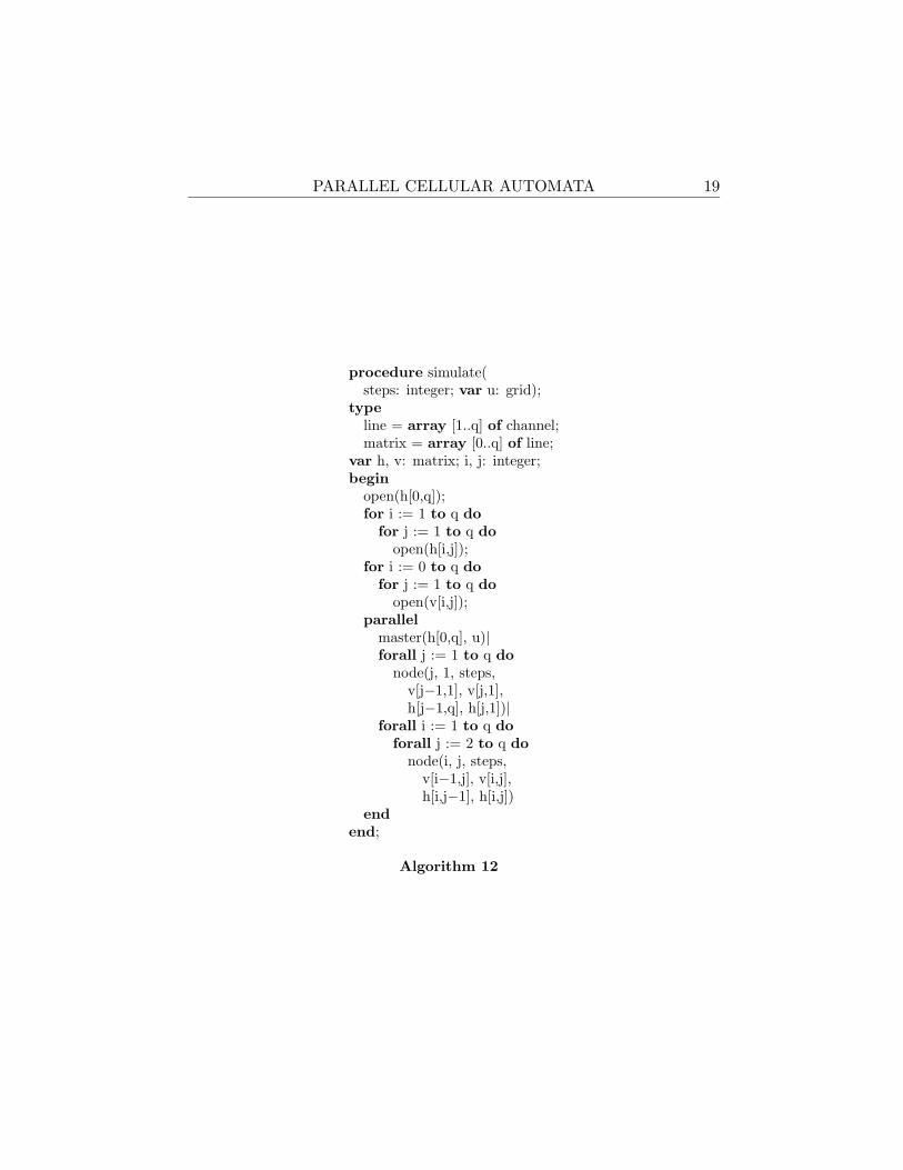
PARALLEL CELLULAR AUTOMATA 19
procedure simulate(steps: integer; var u: grid);
typeline = array [1..q] of channel;matrix = array [0..q] of line;
var h, v: matrix; i, j: integer;begin
open(h[0,q]);for i := 1 to q do
for j := 1 to q doopen(h[i,j]);
for i := 0 to q dofor j := 1 to q do
open(v[i,j]);parallel
master(h[0,q], u)|forall j := 1 to q do
node(j, 1, steps,v[j−1,1], v[j,1],h[j−1,q], h[j,1])|
forall i := 1 to q doforall j := 2 to q do
node(i, j, steps,v[i−1,j], v[i,j],h[i,j−1], h[i,j])
endend;
Algorithm 12
20 PER BRINCH HANSEN
procedure nextstate(var u: subgrid;i, j: integer);{ 1 <= i <= m, 1 <= j <= m }const pa = 0.3; pb = 0.01;var x: real;begin
case u[i,j] ofalive:
if(u[i−1,j] = burning) or(u[i+1,j] = burning) or(u[i,j+1] = burning) or(u[i,j−1] = burning)
then u[i,j] := burningelse
beginrandom(x);if x <= pb then
u[i,j] := burningend;
burning:u[i,j] := dead;
dead:begin
random(x);if x <= pa then
u[i,j] := aliveend
endend;
Algorithm 4.1
PARALLEL CELLULAR AUTOMATA 21
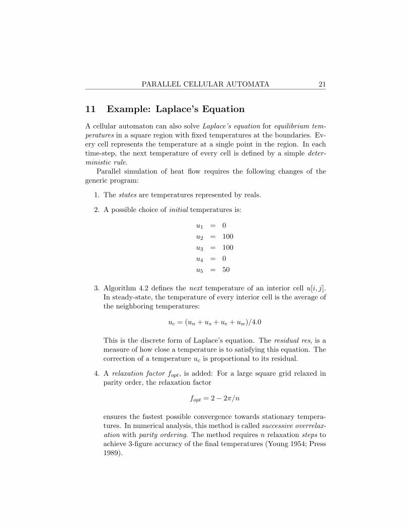
11 Example: Laplace’s Equation
A cellular automaton can also solve Laplace’s equation for equilibrium tem-peratures in a square region with fixed temperatures at the boundaries. Ev-ery cell represents the temperature at a single point in the region. In eachtime-step, the next temperature of every cell is defined by a simple deter-ministic rule.
Parallel simulation of heat flow requires the following changes of thegeneric program:
1. The states are temperatures represented by reals.
2. A possible choice of initial temperatures is:
u1 = 0u2 = 100u3 = 100u4 = 0u5 = 50
3. Algorithm 4.2 defines the next temperature of an interior cell u[i, j].In steady-state, the temperature of every interior cell is the average ofthe neighboring temperatures:
uc = (un + us + ue + uw)/4.0
This is the discrete form of Laplace’s equation. The residual res, is ameasure of how close a temperature is to satisfying this equation. Thecorrection of a temperature uc is proportional to its residual.
4. A relaxation factor fopt, is added: For a large square grid relaxed inparity order, the relaxation factor
fopt = 2− 2π/n
ensures the fastest possible convergence towards stationary tempera-tures. In numerical analysis, this method is called successive overrelax-ation with parity ordering. The method requires n relaxation steps toachieve 3-figure accuracy of the final temperatures (Young 1954; Press1989).
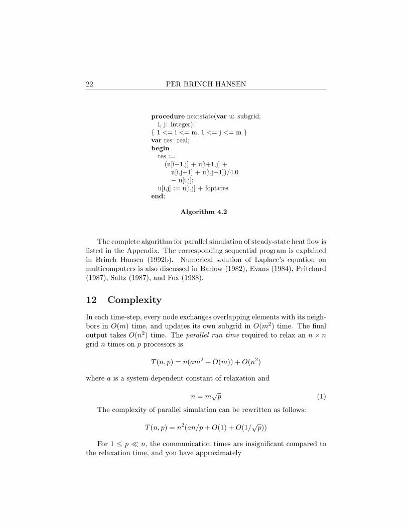
22 PER BRINCH HANSEN
procedure nextstate(var u: subgrid;i, j: integer);{ 1 <= i <= m, 1 <= j <= m }var res: real;begin
res :=(u[i−1,j] + u[i+1,j] +
u[i,j+1] + u[i,j−1])/4.0− u[i,j];
u[i,j] := u[i,j] + fopt∗resend;
Algorithm 4.2
The complete algorithm for parallel simulation of steady-state heat flow islisted in the Appendix. The corresponding sequential program is explainedin Brinch Hansen (1992b). Numerical solution of Laplace’s equation onmulticomputers is also discussed in Barlow (1982), Evans (1984), Pritchard(1987), Saltz (1987), and Fox (1988).
12 Complexity
In each time-step, every node exchanges overlapping elements with its neigh-bors in O(m) time, and updates its own subgrid in O(m2) time. The finaloutput takes O(n2) time. The parallel run time required to relax an n × ngrid n times on p processors is
T (n, p) = n(am2 +O(m)) +O(n2)
where a is a system-dependent constant of relaxation and
n = m√p (1)
The complexity of parallel simulation can be rewritten as follows:
T (n, p) = n2(an/p+O(1) +O(1/√p))
For 1 ≤ p ¿ n, the communication times are insignificant compared tothe relaxation time, and you have approximately
PARALLEL CELLULAR AUTOMATA 23
T (n, p) ≈ an3/p for n À p (2)
If the same simulation runs on a single processor, the sequential run timeis obtained by setting p = 1 in (2):
T (n, 1) ≈ an3 for n À 1 (3)
The processor efficiency of the parallel program is
E(n, p) =T (n, 1)p T (n, p)
(4)
The numerator is proportional to the number of processor cycles used in asequential simulation. The denominator is a measure of the total number ofcycles used by p processors performing the same computation in parallel.
By (2), (3) and (4) you find that the parallel efficiency is close to one,when the problem size n is large compared to the machine size p:
E(n, p) ≈ 1 for n À p
Since this analysis ignores the (insignificant) communication times, it cannotpredict how close to one the efficiency is.
In theory, the efficiency can be computed from (4) by measuring thesequential and parallel run times for the same value of n. Unfortunately,this is not always feasible. When 36 nodes relax a 1500× 1500 grid of 64-bitreals, every node holds a subgrid of 250 × 250 × 8 = 0.5 Mbyte. However,on a single processor, the full grid occupies 18 Mbytes.
A more realistic approach is to make the O(n2) grid proportional to themachine size p. Then every node has an O(m2) subgrid of constant sizeindependent of the number of nodes. And the nodes always perform thesame amount of computation per time-step.
When a scaled simulation runs on a single processor, the run time isapproximately
T (m, 1) ≈ am3 for m À 1 (5)
since p = 1 and n = m.From (1), (3) and (5) you obtain
T (n, 1) ≈ p3/2 T (m, 1) for m À 1 (6)
24 PER BRINCH HANSEN
The computational formula you need follows from (4) and (6):
E(n, p) ≈√p T (m, 1)T (n, p)
for m À 1 (7)
This formula enables you to compute the efficiency of a parallel simulationby running a scaled-down version of the simulation on a single node.
13 Performance
I reprogrammed the model program in occam2 and ran it on a ComputingSurface with T800 transputers configured as a square matrix with a masternode (Meiko 1987; Inmos 1988; McDonald 1991). The program was modifiedto solve Laplace’s equation as explained in Sec. 11. The complete programis found in the Appendix.
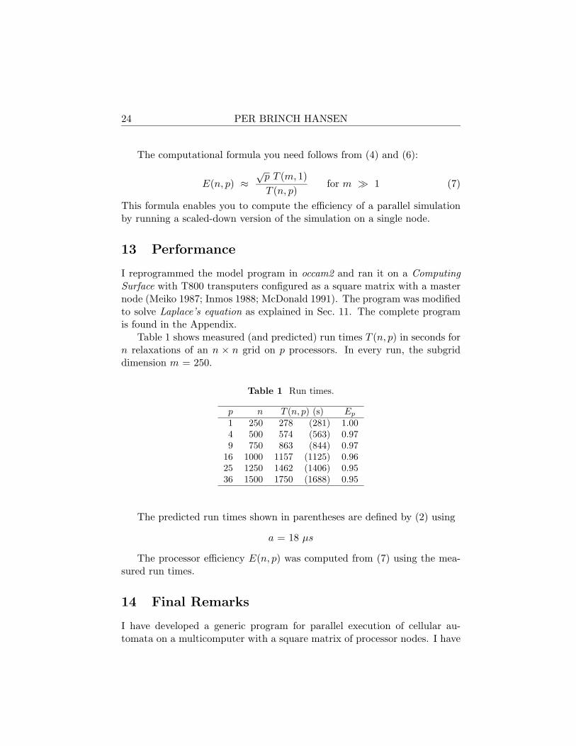
Table 1 shows measured (and predicted) run times T (n, p) in seconds forn relaxations of an n × n grid on p processors. In every run, the subgriddimension m = 250.
Table 1 Run times.
p n T (n, p) (s) Ep1 250 278 (281) 1.004 500 574 (563) 0.979 750 863 (844) 0.97
16 1000 1157 (1125) 0.9625 1250 1462 (1406) 0.9536 1500 1750 (1688) 0.95
The predicted run times shown in parentheses are defined by (2) using
a = 18 µs
The processor efficiency E(n, p) was computed from (7) using the mea-sured run times.
14 Final Remarks
I have developed a generic program for parallel execution of cellular au-tomata on a multicomputer with a square matrix of processor nodes. I have
PARALLEL CELLULAR AUTOMATA 25
adapted the generic program for simulation of a forest fire and numericalsolution of Laplace’s equation for stationary heat flow. On a ComputingSurface with 36 transputers the program performs 1500 relaxations of a1500× 1500 grid of 64-bit reals in 29 minutes with an efficiency of 0.95.
15 Appendix: Complete Algorithm
The complete algorithm for parallel solution of Laplace’s equation is com-posed of Algorithms 1–12.
const q = 6; m = 250 { even };n = 1500 { m∗q };
typerow = array [1..n] of real;grid = array [1..n] of row;
procedure laplace(var u: grid;u1, u2, u3, u4, u5: real;steps: integer);
typesubrow = array [0..m+1] of real;subgrid = array [0..m+1] of subrow;channel = ∗(real);
procedure node(qi, qj, steps: integer;up, down, left, right: channel);
const pi = 3.14159265358979;var u: subgrid; k: integer; fopt: real;
procedure copy(no: integer;inp, out: channel);
var k: integer; uk: real;begin
for k := 1 to no dobegin
receive(inp, uk);send(out, uk)
endend;
26 PER BRINCH HANSEN
procedure output(qi, qj: integer;inp, out: channel; var u: subgrid);
var i, j: integer;begin
for i := 1 to m dobegin
for j := 1 to m dosend(out, u[i,j]);
copy((q − qj)∗m, inp, out)end;
copy((q − qi)∗m∗n, inp, out)end;
procedure phase1(qi, qj, b: integer;up, down, left, right: channel;var u: subgrid);
var k, last: integer;begin
k := 2 − b;last := m − b;while k <= last do
begin{ 1 <= k <= m }[sic] parallel
if qi > 1 thenreceive(up, u[0,k])|
if qi < q thensend(down, u[m,k])|
if qj > 1 thenreceive(left, u[k,0])|
if qj < q thensend(right, u[k,m])
end;k := k + 2
endend;
PARALLEL CELLULAR AUTOMATA 27
procedure phase2(qi, qj, b: integer;up, down, left, right: channel;var u: subgrid);
var k, last: integer;begin
k := b + 1;last := m + b − 1;while k <= last do
begin{ 1 <= k <= m }[sic] parallel
if qi > 1 thensend(up, u[1,k])|
if qi < q thenreceive(down, u[m+1,k])|
if qj > 1 thensend(left, u[k,1])|
if qj < q thenreceive(right, u[k,m+1])
end;k := k + 2
endend;
procedure exchange(qi, qj, b: integer;up, down, left, right: channel;var u: subgrid);
beginphase1(qi, qj, b,
up, down, left, right, u);phase2(qi, qj, b,
up, down, left, right, u)end;
function initial(i, j: integer): real;begin
if i = 0 theninitial := u1
28 PER BRINCH HANSEN
else if i = n + 1 theninitial := u2
else if j = n + 1 theninitial := u3
else if j = 0 theninitial := u4
elseinitial := u5
end;
procedure nextstate(var u: subgrid;i, j: integer);{ 1 <= i <= m, 1 <= j <= m }var res: real;begin
res :=(u[i−1,j] + u[i+1,j] +
u[i,j+1] + u[i,j−1])/4.0− u[i,j];
u[i,j] := u[i,j] + fopt∗resend;
procedure newgrid(qi, qj: integer;var u: subgrid);
var i, i0, j, j0: integer;begin
i0 := (qi − 1)∗m;j0 := (qj − 1)∗m;for i := 0 to m + 1 do
for j := 0 to m + 1 dou[i,j] := initial(i0+i, j0+j)
end;
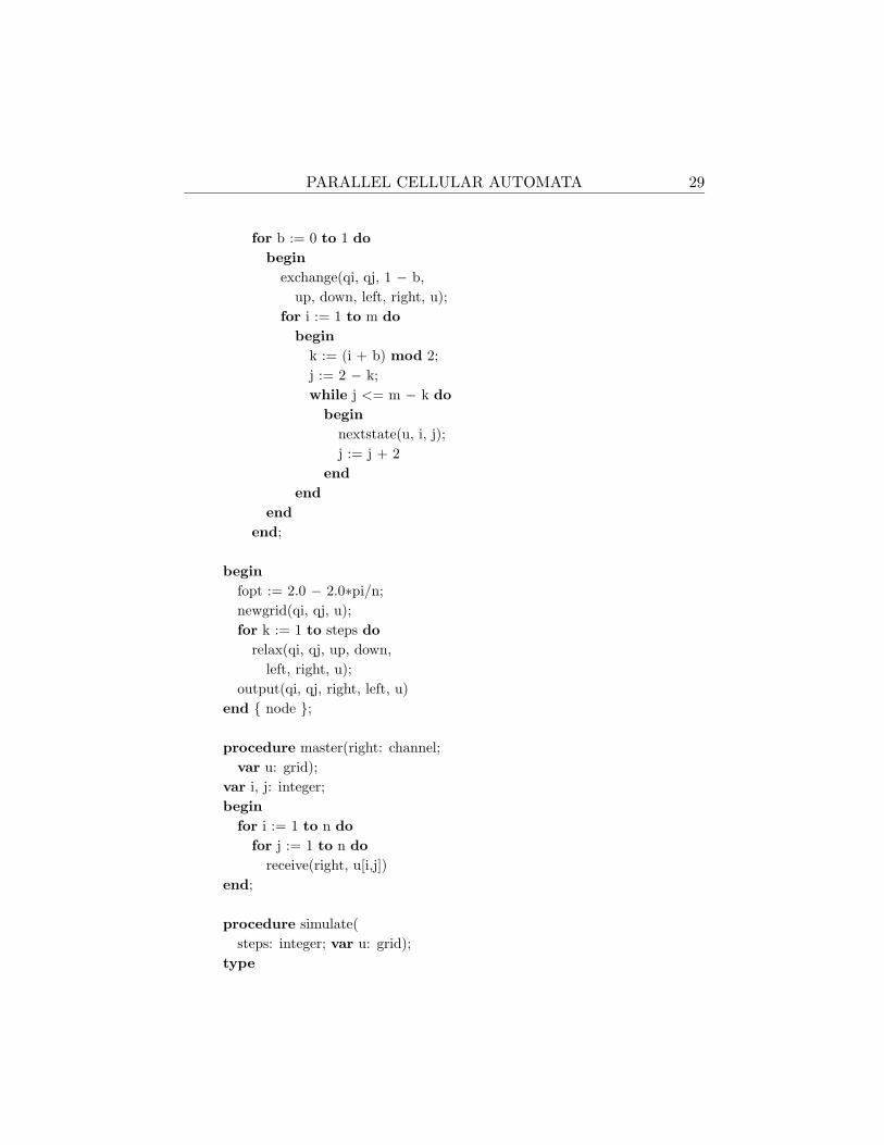
procedure relax(qi, qj: integer;up, down, left, right: channel;var u: subgrid);
var b, i, j, k: integer;begin
PARALLEL CELLULAR AUTOMATA 29
for b := 0 to 1 dobegin
exchange(qi, qj, 1 − b,up, down, left, right, u);
for i := 1 to m dobegin
k := (i + b) mod 2;j := 2 − k;while j <= m − k do
beginnextstate(u, i, j);j := j + 2
endend
endend;
beginfopt := 2.0 − 2.0∗pi/n;newgrid(qi, qj, u);for k := 1 to steps do
relax(qi, qj, up, down,left, right, u);
output(qi, qj, right, left, u)end { node };
procedure master(right: channel;var u: grid);
var i, j: integer;begin
for i := 1 to n dofor j := 1 to n do
receive(right, u[i,j])end;
procedure simulate(steps: integer; var u: grid);
type
30 PER BRINCH HANSEN
line = array [1..q] of channel;matrix = array [0..q] of line;
var h, v: matrix; i, j: integer;begin
open(h[0,q]);for i := 1 to q do
for j := 1 to q doopen(h[i,j]);
for i := 0 to q dofor j := 1 to q do
open(v[i,j]);parallel
master(h[0,q], u)|forall j := 1 to q do
node(j, 1, steps,v[j−1,1], v[j,1],h[j−1,q], h[j,1])|
forall i := 1 to q doforall j := 2 to q do
node(i, j, steps,v[i−1,j], v[i,j],h[i,j−1], h[i,j])
endend;
beginsimulate(steps, u)
end { laplace };
Acknowledgements
It is a pleasure to acknowledge the constructive comments of JonathanGreenfield.
References
Bak, P., and Tang, C. 1989. Earthquakes as a self-organized critical phenomenon. Journalof Geophysical Research 94, B11, 15635–15637.
PARALLEL CELLULAR AUTOMATA 31
Bak, P., and Chen, K. 1990. A forest-fire model and some thoughts on turbulence. PhysicsLetters A 147, 5–6, 297–299.
Barlow, R.H., and Evans, D.J. 1982. Parallel algorithms for the iterative solution to linearsystems. Computer Journal 25, 1, 56–60.
Berlekamp, E.R., Conway, J.H., and Guy, R.K. 1982. Winning Ways for Your Mathemat-ical Plays. Vol. 2, Academic Press, New York, 817–850.
Brinch Hansen, P. 1990. The all-pairs pipeline. School of Computer and InformationScience, Syracuse University, Syracuse, NY.
Brinch Hansen, P. 1991a. A generic multiplication pipeline. School of Computer andInformation Science, Syracuse University, Syracuse, NY.
Brinch Hansen, P. 1991b. Parallel divide and conquer. School of Computer and Informa-tion Science, Syracuse University, Syracuse, NY.
Brinch Hansen, P. 1992a. Parallel Monte Carlo trials. School of Computer and InformationScience, Syracuse University, Syracuse, NY.
Brinch Hansen, P. 1992b. Numerical solution of Laplace’s equation. School of Computerand Information Science, Syracuse University, Syracuse, NY.
Brinch Hansen, P. 1994. SuperPascal—A publication language for parallel scientific com-puting. Concurrency—Practice and Experience 6, 5 (August), 461–483. Article 24.
Cok, R.S. 1991. Parallel Programs for the Transputer. Prentice Hall, Englewood Cliffs,NJ.
Dewdney, A.K. 1984. Sharks and fish wage an ecological war on the toroidal planet Wa-Tor. Scientific American 251, 6, 14–22.
Dijkstra, E.W. 1982. Selected Writings on Computing: A Personal Perspective. Springer-Verlag, New York, 334–337.
Evans, D.J. 1984. Parallel SOR iterative methods. Parallel Computing 1, 3–18.
Fox, G.C., Johnson, M.A., Lyzenga, G.A., Otto, S.W., Salmon, J.K., and Walker, D.W.1988. Solving Problems on Concurrent Processors, Vol. I, Prentice-Hall, EnglewoodCliffs, NJ.
Frisch, U., Hasslacher, B., and Pomeau, Y. 1986. Lattice-gas automata for the Navier-Stokes equation. Physical Review Letters 56 14, 1505–1508.
Gardner, M. 1970. The fantastic combinations of John Conway’s new solitaire game “Life.”Scientific American 223, 10, 120–123.
Gardner, M. 1971. On cellular automata, self-reproduction, the Garden of Eden and thegame “Life.” Scientific American 224, 2, 112–117.
Hoppensteadt, F.C. 1978. Mathematical aspects of population biology. In MathematicsToday: Twelve Informal Essays, L.A. Steen, Ed. Springer-Verlag, New York.
Hwa, T., and Kardar, M. 1989. Dissipative transport in open systems: An investigationof self-organized criticality. Physical Review Letters 62, 16, 1813–1816.
Inmos Ltd. 1988).occam 2 Reference Manual. Prentice Hall, Englewood Cliffs, NJ.
McDonald, N. 1991. Meiko Scientific Ltd. In Past, Present, Parallel: A Survey of AvailableParallel Computing Systems, A. Trew and G. Wilson, Eds. Springer-Verlag, New York,165–175.
Meiko Ltd. 1987. Computing Surface Technical Specifications. Meiko Ltd., Bristol, Eng-land.
Press, W.H., Flannery, B.P., Teukolsky, S.A., and Vetterling, W.T. 1989. NumericalRecipes in Pascal: The Art of Scientific Computing. Cambridge University Press,Cambridge, MA.
32 PER BRINCH HANSEN
Pritchard, D.J., Askew, C.R., Carpenter, D.D., Glendinning, I., Hey, A.J.G., and Nicole,D.A. 1987. Practical parallelism using transputer arrays. Lecture Notes in ComputerScience 258, 278–294.
Saltz, J.H., Naik, V.K., and Nicol, D.M. 1987. Reduction of the effects of the communi-cation delays in scientific algorithms on message passing MIMD architectures. SIAMJournal on Scientific and Statistical Computing 8, 1, s118–s134.
Ulam, S. 1986. Science, Computers, and People: From the Tree of Mathematics, Birkhauser,Boston, MA.
von Neumann, J. 1966. Theory of Self-Reproducing Automata. Edited and completed byA.W. Burks, University of Illinois Press, Urbana, IL.
Young, D.M. 1954. Iterative methods for solving partial difference equations of elliptictype. Transactions of the American Mathematical Society 76, 92–111.