parallel and distributed adaptive quadrilateral mesh generation

Parallel and distributed adaptive quadrilateral meshgeneration

B.H.V. Topping*, B. Cheng

Department of Mechanical Engineering, Heriot±Watt University, Riccarton, Edinburgh, EH14 4AS, UK

Received 1 October 1996; accepted 3 July 1998

Abstract

A parallel quadrilateral mesh generation using advanced front technology is presented in this paper. An improved

quadrilateral mesh generation technology which uses the advancing front technology was introduced by the authorspreviously. This new quadrilateral mesh generation technique has been developed for use with parallel computingenvironments. The parallel code has been created by adapting the sequential code using each coarse quadrilateral asa sub-domain for remeshing. A transputer-based parallel system and a heterogeneous network of workstations using

the parallel virtual machine system were employed. The use of these parallel environments to improve the e�ciencyof the proposed mesh generator was investigated. Some pre-processes have been introduced to ensure load balancingduring the parallel mesh generation. A post processor has been developed to assist in the assembly of the distributed

portions of the mesh. Four examples are presented to demonstrate the robustness and e�ciency of this parallel meshgenerator. Some nearly linear speed-up curves have been achieved for some large meshes by using up to 11transputers. # 1999 Civil-Comp Ltd and Elsevier Science Ltd. All rights reserved.

1. Introduction

Within recent years, parallel computation has beenwidely exploited in di�erent areas. The object of paral-

lel processing is to improve the processing speed andhopefully the computational e�ciency. An investi-gation has been carried out to apply parallelism to thequadrilateral mesh generation technique presented in

the previous paper [1]. Parallel programs which runusing parallel virtual machine (PVM) and transputerbased systems have been developed by adapting the

sequential quadrilateral mesh generation codedescribed in Ref. [1].

2. Quadrilateral mesh generation

Considerable work has been carried out by Zhu etal. [2] in applying the advancing front technique to

quadrilateral mesh generation. In Zhu et al.'s [2] tech-nique, a more accurate distribution of the desired meshsize can be accomplished by implementing the advan-cing front technique which uses a ``background mesh''

to de®ne the mesh size. This technique produces aquadrilateral by combining two triangles which share acommon side. In this technique, Zhu extended triangle

generation to quadrilateral generation by keeping thetriangle process the same as triangular mesh generationand adding a new process to combine two triangles;

hence all transition triangular elements are produced inthe same way as in triangular mesh generation. Thetransition triangles satisfy the element size distributionbut the ®nal quadrilateral element sizes are not directly

considered. This reduces the control of the mesh size.

Computers and Structures 73 (1999) 519±536

0045-7949/99/$ - see front matter # 1999 Civil-Comp Ltd and Elsevier Science Ltd. All rights reserved.

PII: S0045-7949(98 )00254-5

www.elsevier.com/locate/compstruc

* Corresponding author.

The quadrilateral mesh generation procedure was

improved in Ref. [1]. In Fig. 1 the transition triangles

were generated using the improved method. There are

two ideal points marked Co. Each Co point is gener-

ated along a perpendicular chord from the end-point

of the reference segment. The lengths of the diagonals

are aco2=d1 and bco1=d2 where d1, d2 are the interp-

olated values of mesh parameter at two end-points of

the reference segment. This new triangle generation

makes the quadrilateral element size directly using the

respective element size parameters. For the ®rst tri-

angle generation, the point Co2, which corresponds to

the smaller mesh parameter, will be chosen.

A second point, Co1, is generated for the next tri-

angle along a perpendicular chord from the other end-

point of the reference segment using the corresponding

mesh parameter. A check must be performed to calcu-

late the distance between the point Co1 and the seg-

ment a-Co2. If Co1 is found to be within the ®rst

triangle then Co1 is discarded and replaced with a new

Co1 generated perpendicularly from the mid point of

the segment a-Co2.

The points Co1 and Co2 are now the ideal points,

but they may still not be satisfactory to generate a

quadrilateral element from two triangles. Before these

can be con®rmed as the points to be used to generate

the triangles, the points must be checked to ensure

that:

. The points lie within the domain to be remeshed

and not outside the advancing front, otherwise new

control points must be generated using the conven-

tional approach [3].

. The points generated must not be too close to exist-

ing points otherwise the existing points should be

selected as alternative apex points.

Using the con®rmed points Co2 and Co1 the quadri-

lateral (a±b±Co2±Co1) is formed. This new triangle

generation makes the quadrilateral element sizes

directly accord with the distribution of the desiredmesh size when the original Co1 and Co2 are used for

the quadrilateral generation.This method of generating quadrilaterals is more

precise than the techniques usually used. In Ref. [1] the

methods employed to combine two triangles to form aquadrilateral were discussed. A new approach utilizinga ®ssion element was presented. This technique has

been utilized in the parallel work presented in thispaper.

3. The general architecture of parallel programs

An application consists of a collection of one or

more concurrently executing tasks. Each task maycomprise one or more threads and it has its ownregion of memory for code and data, a vector of input

ports and a vector of output ports. Tasks can be trea-ted as building blocks for parallel systems. The con-®guration software provides ways of specifying whichsoftware tasks are to be run on which processors. Each

processor can support any number of tasks, limitedonly by the available memory.The 3L Parallel C compiler [4] was used for the

development of this parallel mesh generation version.This compiler has most of the ANSI features. Thecompiler is based on the same abstract model of com-

municating sequential processes as the transputer hard-ware. The extension to support parallel computationsis provided in the runtime library and in con®gurer

arrays. Further details on transputer systems may befound in Ref. [5].

3.1. Processor farming parallel environment

In the processor farming environment each pro-cessor in the network carries the same code and exe-

cutes it in isolation from all the other processors. Thisis also termed independent task or event parallelism.The parallel adaptive mesh generator developed in this

paper is based upon this form of parallelism. Thereason for implementing it is explained in Section 6.When using the processor farming environment the

code is generally divided into a master task code and

one or more worker task codes. All the worker tasksmay have an identical code or di�erent codes. In trans-puter based parallel processing systems the processor

which connects the transputer network to the host, e.g.a personal computer or workstation, is called the rootprocessor. This processor executes the master task

code and may also execute one or more work taskcodes. The master task is generally written to performthe following functions:

Fig. 1. Quadrilateral generation using the new triangular gen-

eration.

B.H.V. Topping, B. Cheng / Computers and Structures 73 (1999) 519±536520

1. Perform any input/output required by the worker

tasks.2. Split the job into work packets which can be

handled independently by the ``farm workers''.3. Receive ``results'' packets from the worker tasks

during the execution of worker task codes on theparallel processors.

The worker tasks generally perform the following func-

tions:

1. Receive the data from the master task.2. Perform computations.

3. Send intermediate results, if necessary, to the mastertask.

4. Send the ®nal results to the master task.

The master and worker tasks are compiled separately.The compiled tasks are then linked using the corre-sponding linker which is available within the compiler,

but the master and worker linking procedures aredi�erent. The master should be linked with the stan-dard run-time library. The worker task must be linked

with the stand-alone run-time library.A ¯ood±®ll application has the advantage of being

able to run on di�erent numbers of transputers with-out making any changes to the con®guration ®le or re-

con®guring the bootable ®le [4]. Thus the source codesproduced using the ¯ood±®ll con®gurer are completelyportable.

4. Introduction to parallel virtual machine

The parallel virtual machine (PVM) is a softwaresystem that allows the utilization of a heterogeneous

network of parallel and serial computers as a single

computational resource [6]. In other words, using thePVM environment, the user can run a number of pro-cesses on di�erent machines as easily as on one ma-chine. This system provides a convenient facility to

maximize the power of existing networked machines.

4.1. PVM architecture

A PVM may be applied on a hardware base consist-

ing of di�erent machines and architectures, includingsingle CPU systems, vector machines and multiproces-sors [8]. Many local networks may be interconnected

with each other as one parallel virtual machine. All ofthese machines are accessed by applications via a stan-dard interface that supports common concurrent pro-

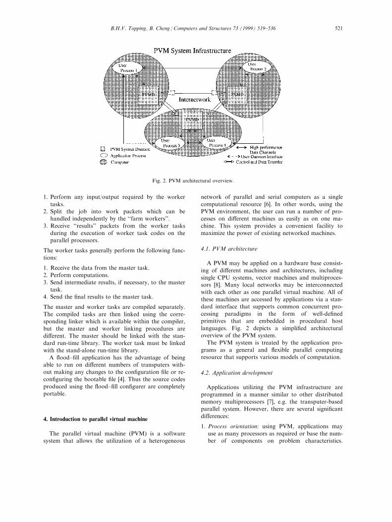
cessing paradigms in the form of well-de®nedprimitives that are embedded in procedural hostlanguages. Fig. 2 depicts a simpli®ed architecturaloverview of the PVM system.

The PVM system is treated by the application pro-grams as a general and ¯exible parallel computingresource that supports various models of computation.

4.2. Application development

Applications utilizing the PVM infrastructure areprogrammed in a manner similar to other distributed

memory multiprocessors [7], e.g. the transputer-basedparallel system. However, there are several signi®cantdi�erences:

1. Process orientation: using PVM, applications mayuse as many processors as required or base the num-ber of components on problem characteristics.

Fig. 2. PVM architectural overview.

B.H.V. Topping, B. Cheng / Computers and Structures 73 (1999) 519±536 521

Unlike processor-oriented parallel machines, processto processor mapping need not be one-to-one.

2. Multiple component exception: inherent support isprovided for cooperative execution of multiple ap-

plication modules (i.e. di�erent programs) each ofwhich may be replicated on hardware multiproces-sors. However cumbersome programming or manual

intervention is required to accomplish this.3. Exploiting heterogeneity: since multifaceted virtual

machines can be con®gured within the same frame-

work, the potential for siting sub tasks on the bestsuited architectures is signi®cantly enhanced.

4. Logical interconnection: for both synchronizationand communication, direct logical visibility is pro-

vided between arbitrary sets of component pro-cesses. Interaction is via a logically complete graphand synchronization points may be assigned abstract

symbolic names.

5. Hardware and software used for the heterogenous

system

The requirements of hardware and software for this

quadrilateral mesh generator in PVM are as follows.The PVM software implemented in this work is version3. It has many improvements over version 2. PVM was

originally developed to join machines connected by anetwork into a single logical machine. Some of thesehosts may themselves be parallel computers with mul-

tiple processors connected by a proprietary network orshared-memory. With PVM 3 the dependence onUNIX sockets and TCP/IP software is relaxed. Forexample, programs written in PVM 3 can run on a net-

work of SUNs, on a group of nodes on an IntelParagon, on multiple Paragons connected by a net-work, or a heterogeneous combination of multiproces-

sor computers distributed around the world withouthaving to write any vender speci®c message-passingcode. PVM 3 is designed to use native communication

calls within a distributed memory multiprocessor orglobal memory with a shared memory multiprocessor.Messages between two nodes of a multiprocessor go

directly between them while messages destined for amachine out on the network go to the user's single

PVM daemon on the multiprocessor for further rout-ing. The networked machines used in this study arefour Sun workstations. Their architectures and ver-

sions are listed in Table 1.

6. Parallel quadrilateral mesh generation

The parallel algorithms implemented currently onmultiple instructions multiple data machines such as

transputer-based systems may be classi®ed brie¯y asfollows:

1. Processor farming, in which each processor in thenetwork carries the same code and di�erent data

and executes it in isolation from all the otherworker processors.

2. Geometric parallelism, in which each processor exe-

cutes the same code on data corresponding to asub-region of the system being simulated and com-municates boundary data to neighbouring pro-

cessors handling neighbouring sub-domains.3. Algorithmic parallelism, in which each processor is

responsible for part of the algorithm and all the

data passes through each processor.

The advancing front technique has proved to be robustand versatile when applied to complicated domain.

For large problems the computation may be very timeconsuming, although some advanced data manipu-lation and search algorithms are used. Most of thecomputational cost is incurred in the following pro-

cedures:

1. Searching for the smallest segment in the activefronts for the new element generation. This is done

by checking all the segments in all active fronts.2. Interpolating new element mesh parameters over the

background grid. This is done by searching the

background elements using corresponding search al-gorithm.

3. Determining all the active nodes which lie within

the circle with the centre at ideal node C and radiusnd. These nodes are ordered according to their dis-tance from C. This is done by calculating the pos-itions of all active nodes.

4. Selecting the apex point from the required candidate(active) points list ni. This list includes both existingnodes and new generated nodes. A point can only

be selected as the apex point for the triangle if itsatis®es conditions such that the element formeddoes not intersect any existing sides in the front.

The process starts from the ®rst candidate point andchecks the points one by one. Once a point is foundthat satis®es the conditions, this point is chosen to

Table 1

Networked workstations used for the distributed mesh gener-

ation in this paper

PVM ARCH Machine version Memory available

SUNMP SS10 128 MB

SUN4SOL2 SPARC IPC 24 MB

SUN4SOL2 SS20 64 MB

SUN4SOL2 SS10 32 MB


be the apex point and the whole process is termi-

nated.

As described before, the advancing front method relies

heavily on having the above procedures applied to the

background mesh and the advancing fronts. These

have to be done for every element generated, hence the

time taken is expensive. As the number of the elements

in the background mesh and the relative size of the

domain increases these procedures become extremely

time consuming.

Considering the issues above, the parallel algorithm

for quadrilateral mesh generation was formulated in

the following ways:

1. To implement the ®rst algorithm (processor farm-

ing), all elements which are in the present mesh are

treated as new sub-domains and are sent to worker

processors for remeshing. The mesh generation pro-

cess would be done in parallel and the algorithm

would not require communication between slave

processors, as each individual slave processor would

be entrusted with a separate sub-domain. However,

the generation of new elements larger than those in

the initial coarse mesh would not be possible in the

parallel quadrilateral mesh generation.

2. To implement the second algorithm (geometric par-

allelization), the mesh generation process is similar

to the ®rst algorithm, but intermediate communi-

cation may be permitted. This communication could

take the form of message passing to permit the

enlargement of elements over subregions. The ®rst

algorithms is obviously more e�cient since there is

no communication between worker processors. This

could lead to the approach of applying the full

advancing front technique to complete subregions

consisting of a number of elements.

3. To implement the third algorithm, the sequential

advancing front method would be adapted to form

a parallel code where di�erent parts of the method

would be carried out on di�erent processors. It is

unlikely that this approach would result in any e�-

ciency because of the amount of processor com-

munication required.

After considering the above three algorithms, the ®rst

algorithm was selected for implementation. This algor-

ithm does not require inter-processor communication

hence a processor farming environment generated by

the ¯ood-®ll con®gurer was selected for the develop-

ment of this algorithm. The same algorithm, which is

called a dynamic loading scheme, was selected for the

PVM parallel computation. It is similar to the pro-

cessor farming algorithm in that the master program

creates and holds the ``pool'' and farms out tasks left

in the pool. Four bene®ts result from applying this al-

gorithm:

1. The total domain is discretized into regular quadri-lateral shaped sub-domains and within each sub-

domain the mesh density will not generally changetoo signi®cantly so the mesh generation procedure issimpli®ed.

2. In the sequential code, the elements size parameterd, is determined by searching the total backgroundmesh. In the parallel code all the remeshing el-

ements are within the corresponding original sub-domain quadrilateral, and hence the element par-ameter was determined using the following formula:

l5 �Xn�4n�1�ln� �1�

l` � 3 � l5 �2�

ai �Xn�4n�1

�l5 ÿ lnl`

an

��3�

if �ai<0:55 � li � ai � 0:55 � li

if �ai > 2 � li � ai � 2 � liwhere ln is the side length of the sub-domain, an isthe nodal parameters of the sub-domain, ai is the in-terpolated value for the new element, li is the rel-

evant active front length, and l5 is the sum of lengthof boundary segments. Since all ai are identical, theprocedure of searching the background mesh is

eliminated.3. Each sub-domain has smaller fronts with fewer seg-

ments and boundary nodes than the entire domain,

so the geometric searching e�ort required to gener-ate an element within a sub-domain is reduced inproportion to the ratio between the size of the sub-

domain and the complete domain.4. As each sub-domain undergoes independent gener-

ation of elements, the actual process of element gen-eration occurs simultaneously within di�erent

regions of the domain.

Before implementing the ®rst algorithm the followingimportant points have to be considered:

1. The discretized background mesh which representsthe domain has to be divided into separate sub-domains, so they can be mapped on di�erent pro-

cessors. The size and shape of each sub-domainshould be such as to measure adequate load balan-cing of the processors for optimizing e�ciency.

2. After the boundary nodes generation, an even num-ber of boundary fronts within each sub-domainmust be guaranteed.


3. The integrity of the boundary connectivities betweenthe meshes generated on separate processors has to

be guaranteed.

7. Pre-processes required before distribution

As each sub-domain is to be remeshed individuallyon a separate processor and the topology of each sub-

domain is known to be quadrilateral, the boundarynodes in all the sub-domains may be numbered identi-cally and in the same order. In other words, each pro-

cessor will receive data which comprises four nodescoordinates and boundary connectivities in a counter-wise manner. This eliminates the requirement for trans-mitting information about the boundary segments of

adjacent sub-domains.The worker processors perform the remeshing pro-

cess and send the generated elements back to master

processor. The ®nal mesh is assembled by the mastertask. Before distribution of the elements or subdo-mains to the processors, two pre-procedures must be

applied to ensure that:

1. Each sub-domain has an even number of boundarynodes.

2. Load balancing must be considered to achieve maxi-mum e�ciency of the parallel computation.

7.1. Generation of boundary nodes

The boundary nodes generation for the parallelmesh generator is quite di�erent from the sequentialcode. In the sequential code the number of boundarynodes for the complete domain should be even,

whereas the number of boundary nodes in each sub-domain must be even for the parallel version. Thequestion of how to ensure that each sub-domain has

an even number of boundary nodes without therequirement to generate large numbers of uneconomicelements is a key point when writing the parallel code.

For the quadrilateral mesh generation, there is abasic requirement that the number of boundary seg-ments or the number of boundary nodes in the frontmust be even. In the conventional advancing front

technique, if after the boundary nodes generation thenumber of boundary nodes is odd, then an additionalnode is added at the end of the last segment. For the

parallel mesh generation the situation is more compli-cated. Each sub-domain is a separate domain andmust be guaranteed an even number of boundary

nodes. As each sub-domain shares boundaries withother sub-domains, modi®cation of the boundarynodes of one sub-domain will in¯uence the boundary

nodes of other sub-domains. One simple method to

handle this problem is to generate an even number ofboundary nodes in each boundary segment. There aretwo disadvantages of this method. First, it makes

further remeshing processing inevitable for all sub-domains, even if some sub-domains have alreadyachieved the permitted error and do not need further

remeshing. Second, many more elements will be gener-ated by the parallel code than the sequential code. An

alternative approach is to generate an odd number ofboundary segments within each sub-domain boundarysegment. A second simple method to solve this pro-

blem is to generate an odd number of segments (oreven number of nodes) on each of the sub-domainboundary segments. This will automatically result in

an even number of segments within the sub-domainfront. This method is superior to the ®rst one because

a non-generative element does not require the additionof further nodes and much re-meshing will be avoided.Using the ®rst method an intermediate node has to be

added to each front to make the number of nodes odddespite the fact that additional nodes may not berequired to reduce the error in the element. With the

second method, further mesh generation is not under-taken in a non-generative element which is sent directly

to the assembler within master task to build the ®nalmesh.The requirement of ensuring an even number of

boundary nodes in the sub-domain front means thatthe meshes generated using the sequential and parallel

codes are generally di�erent. More elements may begenerated in parallel code than the sequential codebecause of the additional nodes that may be generated

on the front.With the advancing front method, an existing node

which satis®es the no-intersection criteria will be

selected to form a new element even if its longest sidelength is longer than d (<1.5 � d ). This means that

geometric criteria are relaxed when using the advan-cing front technique. In the parallel boundary nodegeneration, a similar relaxation technique is used to

manage the boundary segments which must have anodd number of segments on each original sub-domainboundary segment. A node may be added or sub-

tracted to make the number of nodes even. In this im-plementation the number of segments is always

reduced. For example, if four boundary segments aregenerated within an original boundary segment, thenthe last intermediate node may be removed to make

the total boundary fronts equal to three. This reducesthe number of segment nodes from ®ve to four. Afterremoval of a node the remaining boundary nodes are

repositioned. This relaxation eliminates generating une-conomic elements in the parallel remeshing.

For comparison between the parallel and thesequential code, a square domain was selected for


mesh generation using the sequential and parallel

codes. The element size parameter dn=11.0 was ®xedfor both the background mesh elements, the overall

dimensions of the domain being 100 by 100 units. The

mesh which was produced by parallel code comprised

150 nodes and 113 elements, shown in Fig. 3. Themesh which was produced by sequential code com-

prised 126 nodes and 97 elements, shown in Fig. 4.

The di�erence between the number of nodes is 17.5%.

7.2. Processor load balancing

The executable ®le generated by the ¯ood±®ll con®g-urer places the master task and one copy of the workertask on the root transputer and distributes copies of

the worker task to any other transputers connected tothe root. It sends the work packets to the farm ofworker tasks by calling net send. The master simply

does this as fast as it can: whenever the network ofworker tasks becomes saturated, net send is automati-cally blocked until a worker task becomes idle.

Because the routing software is bu�ered, the networkcan hold a number of packets waiting to be processed;this ensures that processors are idle for as short a timeas possible. Even though the ¯ood±®ll con®gurer has

this feature which attempts to keep the network loadbalanced automatically, some crucial points stillremain to be addressed. For example, consider the

situation where a sub-domain will generate a largenumber of elements on remeshing and other sub-domains that will generate fewer elements on remesh-

ing and the total number of sub-domains is small. Inthis case the parallel mesh generation time will dependheavily on the sub-domains, which generates a large

number of elements. The imbalance weakens the paral-lel computational e�ciency. To alleviate this type ofload imbalance, a pre-processor was developed. It sub-divides the sub-domains, which will generate a large

number of elements, into smaller ones. Before remesh-ing the sub-domain the exact number of elementswhich will be remeshed in it will be unknown. In Ref.

[9] the following formulas were suggested:

ratio � davg

Lavg

�4�

Fac1 � Fac

�y30ÿ 1

��5�

if ratio < Fac1, then the relevant sub-domain is dividedinto more sub-domains.In this paper, the above formulas were modi®ed. In

the mesh generation the number of elements which willbe generated depends heavily on the smallest mesh par-ameter of the four boundary nodes. For example, con-sider a boundary segment for two di�erent cases. In

the ®rst case the mesh parameters d1 and d2 of the twoboundary node points are equal to 1 and 0.1. The davgis therefore 0.55. In the second case the smaller mesh

parameter was changed from 0.1 to 0.001 and the newdavg is therefore 0.505. It is obvious that these two davgvalues are almost the same, hence so are the values of

ratio and Fac1. The number of boundary nodes whichwill be generated in this segment of two cases will bequite di�erent. In other words, there will be many

Fig. 3. Mesh produced by parallel code comprising 150 nodes,

113 elements.

Fig. 4. Mesh produced by sequential code comprising 126

nodes, 97 elements.


more intermediate nodes generated in the second casethan in the ®rst case. In order to make the element

parameters more sensitive dn was used instead of davg:

ratio � dnLavg

�6�

where

1

dn�Xi�4i�1

1

dni�7�

Fac1 � Fac

�ymin

60ÿ 1

��8�

where Fac is a parameter whose value has been takenfrom the range 0.1±0.3, Lavg is the average of sub-

domain of four segment lengths, 1/dn is the sum ofinverts of four nodal parameters, and ymin is the mini-mum inter angle of sub-domain.

1. If 0.5 � Frac1 < ratio < Frac1, then the sub-domainis divided into two sub-domains.

2. If ratio < 0.5 � Frac1 then the sub-domain isdivided into ®ve sub-domains.

The details of the subdivision are shown in Fig. 5.Care must be taken to ensure that subdivision doesnot take place if the minimum angle of the sub-domain

is less than 608.

8. Post-processing

The entire mesh is assembled in the master task byassembling each re-meshed element received from theworker tasks. Since the adjacent elements (sub-

domains) of the background mesh share the samenodal mesh parameter values di at the common nodesand the discretization of the boundary segments of the

sub-domains is carried out from the higher value of dito its lower value, the common boundaries of the adja-cent sub-domains will always have the same number

and distribution of intermediate generated nodes. Theassembler accomplishes the new mesh assembly by

comparing each node position of the new element withthe nodes which have been assembled. If this node isclose enough to one of the existing nodes (using a tol-

erance factor), it will be replaced by the correspondingexisting node. Otherwise it will be added into the listof existing nodes as a new node and is assigned a new

number. Thus the common boundary nodes of di�er-ent sub-domains are guaranteed to have the same pos-itions in the ®nal mesh.

9. Structure of parallel quadrilateral mesh generation

code

The parallel mesh generator is created in the form oftwo main programs called master task and workertask.

9.1. Master task

The jobs which the master task undertakes are as

follows:

1. Reads the data of the background mesh from thehost and splits the remeshing job to all transputers.

The packet which is sent to the worker tasksincludes the sub-domain four node coordinates andnodal mesh parameter values.

2. Creates two threads which communicate the back-ground elements to the worker task by using thefunction element send and receives the newly gener-

ated elements from the worker tasker using thefunction element receive. These threads are synchro-nized using a semaphore.

3. The thread element send contains the function net

send which transmits the information packet per-taining to each sub-domain. The router tasks distri-bute these packets among the idle worker tasks.

Whenever the network of worker tasks becomesfully engaged the net send is blocked until a routertask with an empty bu�er becomes available.

4. The thread element receive contains the function netreceive. The results from the worker tasks arereceived and net receive waits until the next packetfrom the worker task becomes available. The net

receive is performed within a never-ending loop.5. Displays the errors on the monitor and terminates

the whole process if the worker tasks encounter

errors.6. During the sending and receiving of sub-domains

the thread deschedule function, from the thread

main, is used to monitor the progress of the remesh-ing. Once all the sub-domains have been received bythe main task then the thread deschedule permits the

Fig. 5. Subdivision of element abcd to two elements (as left

®gure) with abed and bcde, or to ®ve elements (as right).


mesh assembly to proceed. The thread main createstwo threads, background sent and element receive.

Including thread deschedule there are three synchro-nized threads running. The thread main waits forthe worker tasker to complete and send all the pack-

ets and then assembles the whole mesh and writesthe results to an output ®le.

7. The element packets received from the workers are

assembled into the overall mesh by the functionasemble.

9.2. Worker task

The worker task in the ¯ood±®ll con®guration isreplicated at all the nodes of the transputer network.The worker tasks of the parallel mesh generator per-

form the following functions:

1. Receive the packets from the master task.2. Generate boundary nodes and fronts.

3. Every time a sub-domain has been remeshed, it isimmediately transmitted back to the master taskusing the function net send. This procedure creates a

series intermittent communication avoiding the con-gestion of sending all the remeshing data at the endof the process.

4. When a worker task encounters an error, it sends apacket which includes the error ID to the mastertask. The master task then displays the error mess-age on the monitor and terminates all the pro-

cedures.5. When a transputer has accomplished the sub-

domain mesh generation, it sends a ®nal packet

which includes the ®nish signal to master task. Themaster task then counts the number of ®nished sub-domains and sends a new packet to this transputer

is any remain to be remeshed.6. After ®nishing a packet, the worker task returns to

the receiving stage of the code to prepare to receive

the next sub-domain.

9.3. Master±worker communication

There are two data structures used for inter-pro-

cessor communication. The data structure used to

transfer data from the master task to a work taskshould contain all necessary information relating to

the sub-domains. In this paper, each element of thebackground mesh is treated as one sub-domain, sothat all of the sub-domains are quadrilaterals. They

have a regular structure. A data structure called inpacket is used to transfer data from the master task toa worker task. It contains:

1. x[4], four nodal x coordinates.2. y[4], four nodal y coordinates.3. a[4], four nodal mesh parameters.

The maximum length of message the net send cantransfer is 1024 bytes which equals 256 ¯oating pointnumbers. The data structure used here to re¯ect the

results back is a ¯oat array called out packet. It is a¯oat array with a size of 256. The function net sendcan transfer up to 32 remeshing elements each time

and this alleviates the message passing congestion.The protocol to re¯ect results back to master task is

as follows:

1. Pack the remeshing elements in a ¯oat array whichhas a size of 256 numbers. Every time it can sendup to 32 elements back.

2. Once the packing is ®nished, it sets a ®nishing signal

to seal the whole message.3. The master task receives messages from the worker

tasks and stores them. Once it receives a ®nishing

signal from the worker task, it stops reading thismessage and increments the number of remeshedsub-domains by one, indicating that another sub-

domain is complete.

For some large meshes speed-up of up to nine wasachieved by using 11 transputers.

10. Examples

Examples which are given in this section demon-strate the robustness and e�ciency of this parallel

mesh generator for quadrilateral in two-dimensionalproblems. The ®nite element error estimator appliedhere is the simple error estimator from Ref. [4].The ``speed-up'' is de®ned as the ratio of the time

taken by the parallel code to execute on a single pro-

Table 2

Summary of the four examples

Example Problem Original mesh No. of elements First adaptive mesh No. of elements Second adaptive mesh No. of elements

Square Fig. 6 Fig. 7 126 Fig. 8 720 Fig. 9 6859

Cantilever Fig. 13 Fig. 14 7 Fig. 15 113 Fig. 17 517

L-plate Fig. 20 Fig. 21 7 Fig. 22 119 Fig. 26 5426

Hook Fig. 29 Fig. 30 28 Fig. 31 284 Fig. 33 1317


cessor to the time taken to execute on n number ofprocessors. For transputer-based systems, the runtimes were counted by running this program on a net-work of T800 transputers mounted in a PC. For the

PVM runs, the times were counted by running themon various networked machines. The four examplesstudied are summarized in Table 2.

10.1. Example 1

A square domain having a hole in the middle under

the action of horizontal and vertical loads as shown in

Fig. 6. The ®rst uniform mesh had 126 elements and196 nodes as shown in Fig. 7. From the adaptiveanalysis the overall percentage domain error was28.3%. The ®rst remeshing mesh had 720 elements and

805 nodes as shown in Fig. 8. The resulting domainerror was 12.4%. The speed-up curve for the secondremeshing is given in Fig. 11. The second remeshing

mesh had 6859 elements and 7092 nodes as shown inFig. 9. The speed-up curve for the second remeshing isgiven in Fig. 12. The de¯ection is shown in Fig. 10.

Fig. 6. A square domain with a hole under the action of hori-

zontal and vertical loads.

Fig. 7. Uniform mesh for a square domain with a hole

(domain error is 28.3%).

Fig. 8. First adaptive mesh for a square domain with a hole

(domain error is 12.4%).

Fig. 9. Second adaptive mesh for a square domain with a

hole.


The run times for second remeshing mesh on 1, 2, 3,

4, . . . , 11 transputers are recorded in Table 3.

10.2. Example 2

The second example is a cantilever beam under theaction of a vertical load as shown in Fig. 13. The in-

itial manually generated uniform mesh had seven el-ements and 16 nodes as shown in Fig. 14. The domainerror was 46.6%. The ®rst adaptive mesh had 113 el-

ements and 140 nodes as shown in Fig. 15. Thedomain error was 22.9%. The speed-up curve for ®rst

remeshing is given in Fig. 16. The second adaptivemesh had 517 elements and 581 nodes as shown in

Fig. 17. The domain error was 13.68%. The corre-sponding speed-up curve is given in Fig. 18. The runtimes for these remeshings are given in Table 3. The

de¯ection is shown in Fig. 19.

10.3. Example 3

The third example was an L shaped structure with avertical load as shown in Fig. 20. The manually gener-ated uniform mesh had seven elements and 16 nodes

as shown in Fig. 21. The domain error was 51.49%.The ®rst remeshing mesh had 119 elements and 146nodes as shown in Fig. 22. The domain error was

25.28%. The speed-up curve is shown in Fig. 23. Thesecond remeshing mesh had 605 elements and 668nodes as shown in Fig. 24. The domain error was

16.8%. The speed-up is shown in Fig. 25. The thirdadaptive remeshing mesh had 5426 elements and 5615nodes as shown in Fig. 26. The ``speed-up'' curve isshown in Fig. 27. The ®rst and second adaptive

remeshing times are recorded in Table 3. The de¯ec-tion is shown in Fig. 28.

Fig. 13. A cantilever beam under vertical load.

Fig. 10. De¯ection of a square domain with a hole (displace-

ment scale 1:1000).

Fig. 12. Speed-up curve for the second adaptive remeshing

mesh of a square domain with a hole.

Fig. 11. Speed-up curve for the ®rst adaptive remeshing mesh

of a square domain with a hole.


10.4. Example 4

For example 4 a machine hook was used as shown

in Fig. 29. The manually generated mesh had 18 el-

ements and 36 nodes as shown in Fig. 30. The domain

error was 59.73%. The ®rst adaptive remeshing mesh

had 284 elements and 344 nodes as shown in Fig. 31.

The domain error was 27.9%. The speed-up curve is

shown in Fig. 32. The second adaptive remeshing mesh

had 1317 elements and 1445 nodes as shown in Fig.

33. The domain error was 15.35%. The corresponding

speed-up curve is shown in Fig. 34. The times for ®rst

and second remeshings are recorded in Table 3. The

de¯ection is shown in Fig. 35.

Table 3

Remeshing times in seconds running on di�erent numbers of T800 transputers

Example 1 Example 2 Example 3 Example 4

No. of transputers Fig. 8 Fig. 9 Fig. 15 Fig. 17 Fig. 22 Fig. 24 Fig. 26 Fig. 31 Fig. 33

1 43 1464 13 90 13 32 1008 38 205

2 23 716 7 46 7 17 507 21 104

3 16 494 7 31 7 12 340 18 69

4 13 375 7 22 6 9 256 15 53

5 10 296 6 19 6 8 205 15 42

6 8 245 6 16 6 7 171 15 35

7 7 210 6 13 6 7 146 14 30

8 8 187 6 12 6 6 128 13 26

9 7 167 6 11 6 6 113 12 24

10 7 161 6 11 6 6 108 12 23

11 7 156 6 11 6 5 101 12 22

Fig. 14. The manually generated uniform mesh of a cantilever

beam (domain error is 46.6%).

Fig. 15. The ®rst adaptive mesh of a cantilever beam (113 el-

ements, domain error is 22.9%).

Fig. 16. Speed-up curve for the ®rst adaptive remeshing of a

cantilever beam.

Fig. 17. The second adaptive mesh of a cantilever beam (517

elements, domain error is 13.69%).


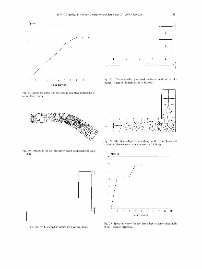
Fig. 18. Speed-up curve for the second adaptive remeshing of

a cantilever beam.

Fig. 19. De¯ection of the cantilever beam (displacement scale

1:1000).

Fig. 20. An L-shaped structure with vertical load.

Fig. 21. The manually generated uniform mesh of an L-

shaped structure (domain error is 51.49%).

Fig. 22. The ®rst adaptive remeshing mesh of an L-shaped

structure (119 elements, domain error is 25.28%).


of an L-shaped structure.


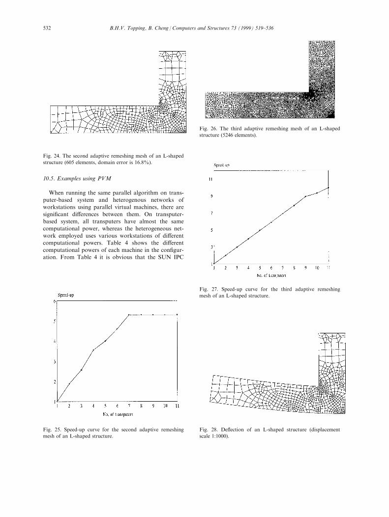
10.5. Examples using PVM

When running the same parallel algorithm on trans-puter-based system and heterogenous networks ofworkstations using parallel virtual machines, there are

signi®cant di�erences between them. On transputer-based system, all transputers have almost the samecomputational power, whereas the heterogeneous net-

work employed uses various workstations of di�erentcomputational powers. Table 4 shows the di�erentcomputational powers of each machine in the con®gur-ation. From Table 4 it is obvious that the SUN IPC

Fig. 24. The second adaptive remeshing mesh of an L-shaped

structure (605 elements, domain error is 16.8%).

Fig. 25. Speed-up curve for the second adaptive remeshing

mesh of an L-shaped structure.

Fig. 26. The third adaptive remeshing mesh of an L-shaped

structure (5246 elements).

Fig. 27. Speed-up curve for the third adaptive remeshing

mesh of an L-shaped structure.

Fig. 28. De¯ection of an L-shaped structure (displacement

scale 1:1000).


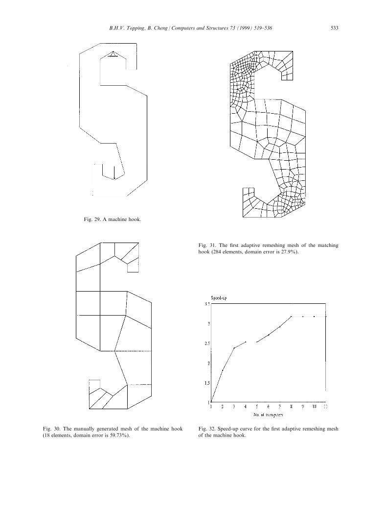
Fig. 29. A machine hook.

Fig. 30. The manually generated mesh of the machine hook

(18 elements, domain error is 59.73%).

Fig. 31. The ®rst adaptive remeshing mesh of the matching

hook (284 elements, domain error is 27.9%).


of the machine hook.


workstation is six times slower than the SUN Sparc10(4 processors) workstation.

11. Conclusions

The following conclusions may be drawn from theresearch on parallel and distributed mesh generation:

1. Parallel mesh generation using the advancing fronttechnique can be easily undertaken using the pro-cessor farming approach. The use of nodal par-

ameters and the same generation procedures foreach element ensures that the nodes generated alongsub-domain interfaces are the same on each elementboundary regardless of the fact that they are gener-

ated on di�erent processors.2. In order to keep the processor loads in balance,

some pre-processors have been developed. These

pre-processors include:

(a) A ®lter which sends all non-generative elements tothe master assembler to form the new mesh without

being sent to a worker task for remeshing.(b) A load balancing technique in which elements

with low nodal mesh parameters that will generateFig. 34. Speed-up curve for the second adaptive remeshing

mesh of the machine hook.

Fig. 33. The second adaptive remeshing mesh of the machine

hook (1317 elements, domain error is 15.35%).

Fig. 35. The de¯ection of the machine hook (displacement

scale 1:1000).


large numbers of elements are divided into smaller

sub-domains.

These pre-processors ensure satisfactory load balan-

cing so that excellent speed-up may be achieved.

Special attention had to be paid so that subdivision

does not take place if the minimum angle of the sub-

domain is less than 608.3. The bene®ts by using the ¯ood±®ll algorithm with

transputers are:

(a) Eliminating the intermediate communication

between transputers.

(b) Automatically keeping the processor loads as

equal as possible.

(c) Providing portability of the parallel code. Once

compiled the code may be run on any number of pro-

cessors without recompilation.

4. Relaxation was applied to the boundary node

generation. The requirement of an even number of

boundary nodes results in di�erent meshes when using

the sequential code or parallel code. Generally more el-

ements will be generated by parallel code than the

sequential code. This relaxation eliminates the require-

ment to generate many unnecessary elements in the

parallel remeshing.

5. The parallel mesh generator uses the coarse mesh

as sub-domains for remeshing therefore it is impossible

to generate elements with sizes larger than those in the

background elements.

6. The PVM system was found to be an e�cient pro-

gramming route for distributed parallel mesh gener-

ation.

The results obtained show that the use of transputer

systems and heterogeneous networks of workstations

using PVM can improve the performance of the

advancing front method. In comparison with the paral-

lel code on a single processor, high speed-up ratios

have been achieved. The robustness of this parallel

mesh generator has been demonstrated by numerical

examples.

Acknowledgements

Biao Cheng would like to take this opportunity to

thank Heriot±Watt University for awarding him ascholarship from the Alexander Neilson Bequest tomake this research possible. The research described in

this paper was supported by Marine TechnologyDirectorate Ltd research contracts: ``High performancecomputing for marine technology research'' (ref. GR/

J22191); and: ``High performance adaptive ®nite el-ement computations for CAD of o�shore structuresusing parallel and heterogeneous systems'' (ref. GR/

J54017). The research described was also supported bythe Systems Architecture Committee of the UKEngineering and Physical Sciences Research Councilthrough the research contract: ``Domain decompo-

sition methods for parallel ®nite element analysis'' (ref.GR/J51634). The authors would like to acknowledgethe helpful discussions with other members of the

Structural Engineering Computational TechnologyResearch Group (SECT) at Heriot±Watt University.In particular Ardeshir Bahreininejad, JaÂ nos Sziveri,

Joao Leite, Janet Wilson and Colin Seale.

References

[1] Cheng B, Topping BHV. Improved quadrilateral adaptive

mesh generation using ®ssion elements. In: Developments

in Computational Technology for Structural Engineering.

Edinburgh: Civil-Comp Press, 1995. p. 391±401.

[2] Zhu JZ, Zienkiewicz OC, Hinton E, Wu J. A new

approach to the development of automatic quadrilateral

mesh generation. Int J Numer Meth Engng 1991;32:849±

66.

[3] Peraire J, Vahdati M, Morgan K, Zeinkiewicz OC.

Adaptive remeshing for compressible ¯ow computations. J

Comput Phys 1987;72:449±66.

[4] Parallel C user Guide (compiler version 2.1) Reference

manual, 3L Ltd, Livingston, Scotland, 1989.

Table 4

Remeshing times running on di�erent machines using PVM

Workstation processor Fig. 8 Fig. 9 Fig. 15 Fig. 17 Fig. 22 Fig. 24 Fig. 26 Fig. 31 Fig. 33

Running on a single machine Sun Sparc 10(4 procs.) 5 126 1 4 2 4 176 2 11

Sun Sparc 20 7 176 2 7 2 6 235 3 16

Sun Sparc 10 11 237 3 10 3 9 363 4 24

Sun IPC 27 751 6 26 9 22 1276 11 61

Running on multiple machines Sparc 10, 20 5 147 1 6 1 5 207 2 13

Sparc 10, 20, IPC 5 147 1 6 1 5 207 2 13

Sparc 10, 20, 10(4 procs.),

Sun IPC

5 110 1 3 1 3 158 1 8


[5] Topping BHV, Khan AI. Parallel ®nite element compu-

tations. Edinburgh: Saxe-Coburg Publications, 1996.

[6] Beguelin A, Dongarra JJ, Geist GA, Manchek R,

Sunderam VS. A user's guide to PVM parallel virtual ma-

chine. Technical report ORNL/TM-11826, Oak Ridge

National Laboratory, July, 1991.

[7] Schmidt BK, Sunderam VS. Empirical analysis of over-

heads in cluster environments. J Concurrency Practice

Experience, 1993.

[8] Geist GA. Network based concurrent computing on the

PVM system. J Concurrency Practice Experience 1992;4

(4):293±311.

[9] Khan AI, Topping BHV. Parallel adaptive mesh gener-

ation. Comput Systems Engng 1991;2:75±101.


parallel and distributed adaptive quadrilateral mesh generation

Documents