ozone nature

ARTICLESPUBLISHED ONLINE: 28 APRIL 2014 | DOI: 10.1038/NGEO2144

Reduction in local ozone levels in urban São Paulodue to a shift from ethanol to gasoline useAlberto Salvo1* and Franz M. Geiger2

Ethanol-based vehicles are thought to generate less pollution than gasoline-based vehicles, because ethanol emissions containlower concentrations of mono-nitrogen oxides than those from gasoline emissions. However, the predicted e�ect of variousgasoline/ethanol blends on the concentration of atmospheric pollutants such as ozone varies between model and laboratorystudies, including those that seek to simulate the same environmental conditions. Here, we report the consequences of a real-world shift in fuel use in the subtropical megacity of São Paulo, Brazil, brought on by large-scale fluctuations in the price ofethanol relative to gasoline between 2009 and 2011. We use highly spatially and temporally resolved observations of roadtra�c levels, meteorology and pollutant concentrations, together with a consumer demandmodel, to show that ambient ozoneconcentrations fell by about 20% as the share of bi-fuel vehicles burning gasoline rose from 14 to 76%. In contrast, nitric oxideand carbon monoxide concentrations increased. We caution that although gasoline use seems to lower ozone levels in the SãoPaulo metropolitan area relative to ethanol use, strategies to reduce ozone pollution require knowledge of the local chemistryand consideration of other pollutants, particularly fine particles.

Ozone levels are relatively high in São Paulo, with hourlyconcentrations above 75 and 125 µgm−3, respectively, being2.7 and 5.3 times more likely than for PM10 in our sample.

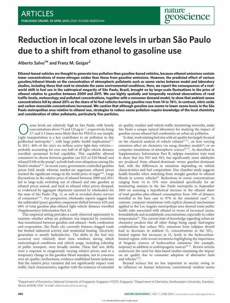
Light transportation is a key contributor to air pollution in thisgridlocked metropolis1–3, with large public health implications4–7.In 2011, 40% of the city’s six million active light-duty vehicles—probably accounting for over one-half of all light-vehicle distancetravelled—possessed bi-fuel capability. This capability allowedconsumers to choose between gasoline (an E25 or E20 blend) andethanol E100 at the pump8, as both fuels were ubiquitous among SãoPaulo’s retailers9,10. In recent years, government-controlled gasolineprices held steady whereas market-set sugarcane ethanol pricestracked the significant swings in the world price of sugar8,10. Largefluctuations in the relative price of ethanol between 2009 and 2011led to large-scale switching out of ethanol and into gasoline asethanol prices soared, and back to ethanol when prices dropped,as evidenced by aggregate shipments reported by wholesalers forthe state of São Paulo (Fig. 1), as well as revealed-choice surveysof consumers11,12. For perspective, wholesaler reports suggest thatthe unblended (pure) gasoline component shifted between 42% and68% of total gasoline-plus-ethanol light-vehicle distance travelled(Supplementary Information Part A).

This empirical setting provides a rarely observed opportunity toexamine whether urban air pollution was impacted by emissionsthat transitioned between gasoline and ethanol—both combustionand evaporation. São Paulo city currently features clogged roadsbut limited industrial activity and residential heating. Electricitygeneration is mostly hydroelectric. The shifts in the fuel mixoccurred over relatively short time windows during whichmeteorological conditions and vehicle usage, including ridershipof public transport, were broadly similar. These fuel mix shiftswere a response to exogenously varying relative prices, and to atemporary change in the gasoline blend mandate, not to concernsover air quality; furthermore, evidence established herein indicatesthat the relative price variation did not significantly impact roadtraffic. Such characteristics, together with the existence of extended

air quality, weather and vehicle traffic monitoring networks, makeSão Paulo a unique natural laboratory for studying the impact ofgasoline versus ethanol fuel combustion on urban air pollution.

To date, work relating fuelmixwith air quality has largely focusedon the chemical analysis of vehicle exhaust13–23, on how varyingemissions affect air chemistry via smog chamber models24, or oncomputer simulations of atmospheric science25–27. As described inSupplementary Information Part B, tailpipe emissions tests tendto show that less NO and NO2 but significantly more aldehydesare produced from ethanol-dominant versus gasoline-dominantfuel, with the differences in emissions depending on vehiclecharacteristics and fuel composition. One chamber study suggestshealth benefits when switching from straight gasoline to ethanolblends in certain vehicles28. Reductions in ozone concentrationsranging from 14 to 55% were simulated specifically for airmonitoring stations in the São Paulo metropolis in September2004 on assessing a hypothetical increase in the ethanol shareof total gasoline-plus-ethanol consumption from 34% of distancetravelled in the base case to 97% in the simulated case25. Incontrast, computer simulations with explicit chemical mechanismsapplied to the Los Angeles metropolitan area showed some publichealth risks associated with ethanol in terms of increased ozone,formaldehyde and acetaldehyde concentrations, especially in coldertemperatures26. The current state of knowledge regarding urban airchemistry predicts that all other things being equal, fuel/enginecombinations that reduce NOX emissions from tailpipes shouldlead to decreases in ambient O3 concentrations in the NOX -limited regime but increases in O3 levels in the hydrocarbon-limited regime, with recent inventories highlighting the importanceof biogenic sources of hydrocarbon emissions (for example,isoprene) in addition to anthropogenic sources29–31. Review articlesunderscore the need for data-based studies examining the impacton air quality due to consumer adoption of alternative fuelsand vehicles32,33.

Beyond science but no less important to society owing toits influence on human behaviour, conventional wisdom seems

1Department of Economics, National University of Singapore, Singapore 117570, Singapore, 2Department of Chemistry, Northwestern University, Evanston,Illinois 60208, USA. *e-mail: [email protected]

450 NATURE GEOSCIENCE | VOL 7 | JUNE 2014 | www.nature.com/naturegeoscience

© 2014 Macmillan Publishers Limited. All rights reserved.

http://www.nature.com/doifinder/10.1038/ngeo2144

mailto:[email protected]

www.nature.com/naturegeoscience

NATURE GEOSCIENCE DOI: 10.1038/NGEO2144 ARTICLES

90

80

70

60

50

40

p e/p

g (%

)

1/10/08

1/1/09

1/4/09

1/7/09

1/10/09

1/1/10

1/4/10

1/7/10

1/10/10

1/1/11

1/4/11

1/7/11

Date

10

9

8

7

6

5

4

3

2

1

0

Ethanol and gasolineshipm

ents (×105 m

3 month

−1)

Gasoline priced favourablyrelative to ethanol in $/km

Ethanol priced favourablyrelative to gasoline in $/km

a

b

0.75

0.50

Gas

olin

e's

shar

e

Figure 1 | Shifting fuel quantities and prices between October 2008 andJuly 2011. a, The monthly share of blended gasoline purchased at retail(E25 or E20) of total estimated light-vehicle distance travelled, preparedfrom wholesale shipment reports. b, The weekly per-litre price of regularethanol (E100), denoted pe, divided by the per-litre price of regular blendedgasoline, denoted pg, at pumps in the city of São Paulo (left y axis). Theblack curve indicates the median, and grey shading represents the ranges ofthe 5th–25th (lower light grey), 25th–75th (dark grey), and 75th–95th(upper light grey) percentile of the distribution of pe/pg across retailers.The 70% ‘parity’ threshold widely reported by the media, at which $ km−1

equalizes, is marked by the dashed blue horizontal line. The right y axisshows monthly reported shipments of all grades of blended gasoline (red)versus ethanol (green) from wholesalers to retailers located in the state ofSão Paulo. Sources: ANP, Inmetro and authors’ calculations.

to associate ethanol with improved environmental outcomes,including air quality (for example, surveys of Brazilian ethanolconsumers12, comments by the ethanol industry at US Senatehearings34,35, and an interview with a former Secretary of theEnvironment in Brazil)9,36. Despite their importance, the abovestudies and claims have not yet been benchmarked against thechemical composition of air measured before, during, and after anactual rather than hypothetical large-scale switch from a fossil fuelover to a biofuel in a large urban centre.

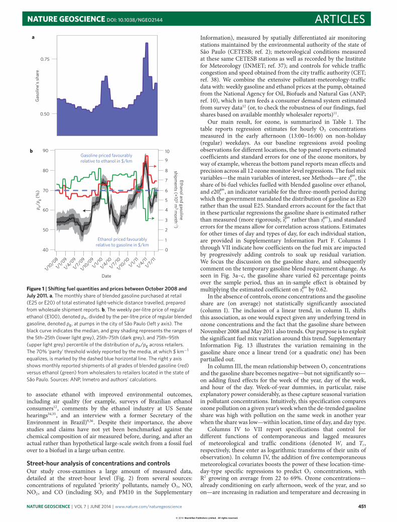
Street-hour analysis of concentrations and controlsOur study cross-examines a large amount of measured data,detailed at the street-hour level (Fig. 2) from several sources:concentrations of regulated ‘priority’ pollutants, namely O3, NO,NO2, and CO (including SO2 and PM10 in the Supplementary

Information), measured by spatially differentiated air monitoringstations maintained by the environmental authority of the state ofSão Paulo (CETESB; ref. 2); meteorological conditions measuredat these same CETESB stations as well as recorded by the Institutefor Meteorology (INMET; ref. 37); and controls for vehicle trafficcongestion and speed obtained from the city traffic authority (CET;ref. 38). We combine the extensive pollutant-meteorology-trafficdata with: weekly gasoline and ethanol prices at the pump, obtainedfrom the National Agency for Oil, Biofuels and Natural Gas (ANP;ref. 10), which in turn feeds a consumer demand system estimatedfrom survey data12 (or, to check the robustness of our findings, fuelshares based on available monthly wholesaler reports)11.

Our main result, for ozone, is summarized in Table 1. Thetable reports regression estimates for hourly O3 concentrationsmeasured in the early afternoon (13:00–16:00) on non-holiday(regular) weekdays. As our baseline regressions avoid poolingobservations for different locations, the top panel reports estimatedcoefficients and standard errors for one of the ozone monitors, byway of example, whereas the bottom panel reports mean effects andprecision across all 12 ozonemonitor-level regressions. The fuel mixvariables—the main variables of interest, see Methods—are sgast , theshare of bi-fuel vehicles fuelled with blended gasoline over ethanol,and e20gast , an indicator variable for the three-month period duringwhich the government mandated the distribution of gasoline as E20rather than the usual E25. Standard errors account for the fact thatin these particular regressions the gasoline share is estimated ratherthan measured (more rigorously, sgast rather than sgast ), and standarderrors for the means allow for correlation across stations. Estimatesfor other times of day and types of day, for each individual station,are provided in Supplementary Information Part F. Columns Ithrough VII indicate how coefficients on the fuel mix are impactedby progressively adding controls to soak up residual variation.We focus the discussion on the gasoline share, and subsequentlycomment on the temporary gasoline blend requirement change. Asseen in Fig. 3a–c, the gasoline share varied 62 percentage pointsover the sample period, thus an in-sample effect is obtained bymultiplying the estimated coefficient on sgast by 0.62.

In the absence of controls, ozone concentrations and the gasolineshare are (on average) not statistically significantly associated(column I). The inclusion of a linear trend, in column II, shiftsthis association, as one would expect given any underlying trend inozone concentrations and the fact that the gasoline share betweenNovember 2008 andMay 2011 also trends. Our purpose is to exploitthe significant fuel mix variation around this trend. SupplementaryInformation Fig. 13 illustrates the variation remaining in thegasoline share once a linear trend (or a quadratic one) has beenpartialled out.

In column III, the mean relationship between O3 concentrationsand the gasoline share becomes negative—but not significantly so—on adding fixed effects for the week of the year, day of the week,and hour of the day. Week-of-year dummies, in particular, raiseexplanatory power considerably, as these capture seasonal variationin pollutant concentrations. Intuitively, this specification comparesozone pollution on a given year’s weekwhen the de-trended gasolineshare was high with pollution on the same week in another yearwhen the share was low—within location, time of day, and day type.

Columns IV to VII report specifications that control fordifferent functions of contemporaneous and lagged measuresof meteorological and traffic conditions (denoted Wt and Tt ,respectively, these enter as logarithmic transforms of their units ofobservation). In column IV, the addition of five contemporaneousmeteorological covariates boosts the power of these location-time-day-type specific regressions to predict O3 concentrations, withR2 growing on average from 22 to 69%. Ozone concentrations—already conditioning on early afternoon, week of the year, and soon—are increasing in radiation and temperature and decreasing in

NATURE GEOSCIENCE | VOL 7 | JUNE 2014 | www.nature.com/naturegeoscience 451




ARTICLES NATURE GEOSCIENCE DOI: 10.1038/NGEO2144

Ibirapuera

Taboão da Serra

São Bernardo do Campo

Parque Dom Pedro II

Parelheiros

São Caetano do Sul

Pinheiros

Osasco

Diadema

Nossa Senhora do Ó

EM Itaquera

IPEN-USP

Santo Amaro

Congonhas

MoócaCerqueiraCésar

Santo André-Paço Municipal

MauáSanto André-Capuava

Guarulhos

Santana

5 km

East

North

West

South

Center

b

1

10

100

1,000

CO(p

pm),

O3 a

nd N

O(µ

g m

−3)

and

radi

atio

n (W

m−2

)

12:00 am

12:00 pm

12:00 am

12:00 pm

12:00 am

12:00 pm

12:00 am

12:00 pm

12:00 am

12:00 pm

12:00 am

12:00 pm

12:00 am

12:00 pm

100

50

0

Traffic congestion (km

)

NO

CO

O3

a

Centro

Mon. 31 Jan. 2011 Tue. 1 Feb. 2011 Wed. 2 Feb. 2011 Thu. 3 Feb. 2011 Fri. 4 Feb. 2011 Sat. 5 Feb. 2011 Sun. 6 Feb. 2011

Figure 2 | Street-hour analysis of concentrations and controls. a, Map of the environmental authority’s air monitoring stations (red squares), which oftendouble as weather stations, in the São Paulo metropolitan area, superimposed on the road network monitored every 30 min by the tra�c authority fortra�c congestion, in São Paulo city. b, Measured concentrations of O3 (blue), NO (brown), and CO (grey), and radiation (yellow), at generic stations andcitywide extension of tra�c congestion (black), by hour from 31 January to 6 February 2011. Sources: CETESB, INMET, CET and ANP.

humidity (a correlate of precipitation) and wind speed. Importantly,the coefficient on the gasoline share, averaged across the 12 O3-monitoring stations, becomes more negative and is more preciselyestimated. Column V also controls for the total extension of trafficcongestion (that is, idling vehicles) reported contemporaneouslyover a monitored 840-km road network across the city. Column VI

adds lagged meteorological and traffic covariates to account forvariation in conditions up to 18 h preceding an observation. Inaddition to road congestion at the citywide level, traffic covariatesin column VI now include two local measures, namely: the sumof congestion only in the region of the city where the monitoringstation is located (for example, North in Fig. 2); and a weighted sum






−100

−50

0

50

100

Ozo

ne c

once

ntra

tion:

net o

f met

, tra

ffic,

sea

sona

lity

and

so o

n(µ

g m

−3)

0.30.20.10.0−0.1−0.2Gasoline share:

Orthogonal to met, traffic, seasonality and so on

200

100

0

Ozo

ne c

once

ntra

tion

( µg

m−3

)

0.70.50.30.1Gasoline share

6

5

4

3

2

1

0

Num

ber o

f reg

iste

red

vehi

cles

(×10

6 )

1/1/09

1/7/091/1/10

1/7/101/1/11

1/7/11

Date

0.8

0.6

0.4

0.2

0.0

Gasoline share

a c

b d

90

80

70

60

50

p e/p

g (%

)

0.750.500.25Fuel share

Gasoline

Ethanol

Slope of best linear predictor = −31.6

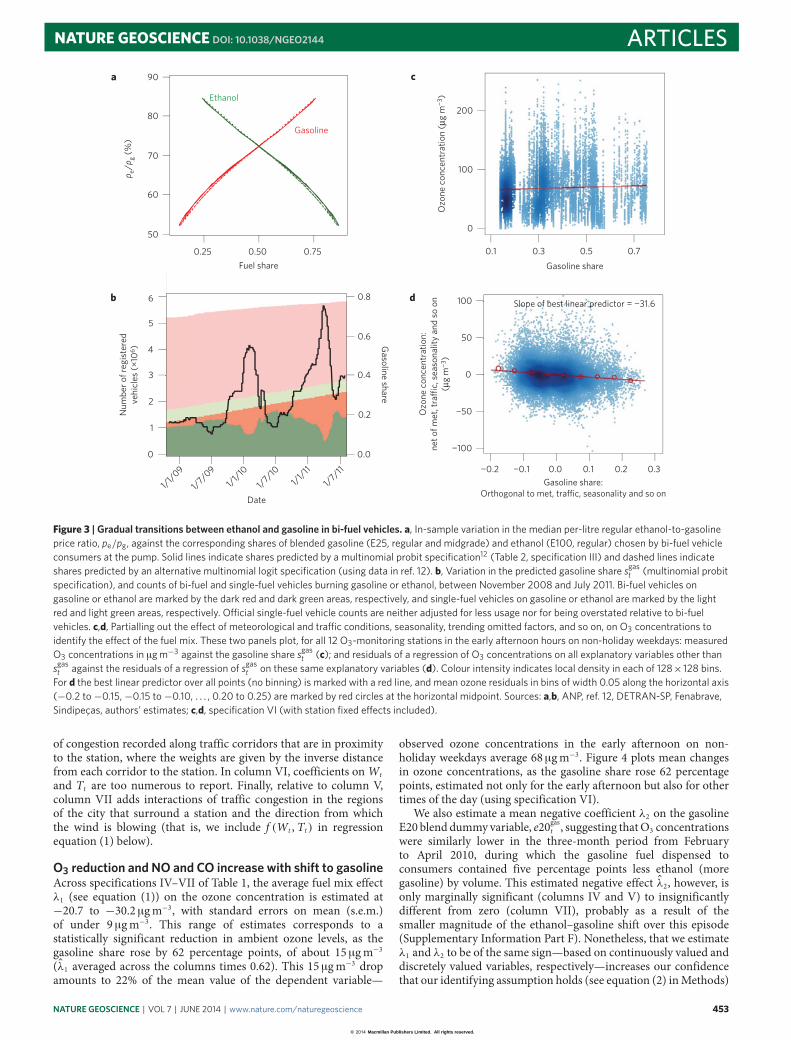
Figure 3 | Gradual transitions between ethanol and gasoline in bi-fuel vehicles. a, In-sample variation in the median per-litre regular ethanol-to-gasolineprice ratio, pe/pg, against the corresponding shares of blended gasoline (E25, regular and midgrade) and ethanol (E100, regular) chosen by bi-fuel vehicleconsumers at the pump. Solid lines indicate shares predicted by a multinomial probit specification12 (Table 2, specification III) and dashed lines indicateshares predicted by an alternative multinomial logit specification (using data in ref. 12). b, Variation in the predicted gasoline share sgas

t (multinomial probitspecification), and counts of bi-fuel and single-fuel vehicles burning gasoline or ethanol, between November 2008 and July 2011. Bi-fuel vehicles ongasoline or ethanol are marked by the dark red and dark green areas, respectively, and single-fuel vehicles on gasoline or ethanol are marked by the lightred and light green areas, respectively. O�cial single-fuel vehicle counts are neither adjusted for less usage nor for being overstated relative to bi-fuelvehicles. c,d, Partialling out the e�ect of meteorological and tra�c conditions, seasonality, trending omitted factors, and so on, on O3 concentrations toidentify the e�ect of the fuel mix. These two panels plot, for all 12 O3-monitoring stations in the early afternoon hours on non-holiday weekdays: measuredO3 concentrations in µg m−3 against the gasoline share sgas

t (c); and residuals of a regression of O3 concentrations on all explanatory variables other thansgast against the residuals of a regression of sgas

t on these same explanatory variables (d). Colour intensity indicates local density in each of 128× 128 bins.For d the best linear predictor over all points (no binning) is marked with a red line, and mean ozone residuals in bins of width 0.05 along the horizontal axis(−0.2 to−0.15,−0.15 to−0.10, . . . , 0.20 to 0.25) are marked by red circles at the horizontal midpoint. Sources: a,b, ANP, ref. 12, DETRAN-SP, Fenabrave,Sindipeças, authors’ estimates; c,d, specification VI (with station fixed e�ects included).

of congestion recorded along traffic corridors that are in proximityto the station, where the weights are given by the inverse distancefrom each corridor to the station. In column VI, coefficients onWtand Tt are too numerous to report. Finally, relative to column V,column VII adds interactions of traffic congestion in the regionsof the city that surround a station and the direction from whichthe wind is blowing (that is, we include f (Wt , Tt) in regressionequation (1) below).

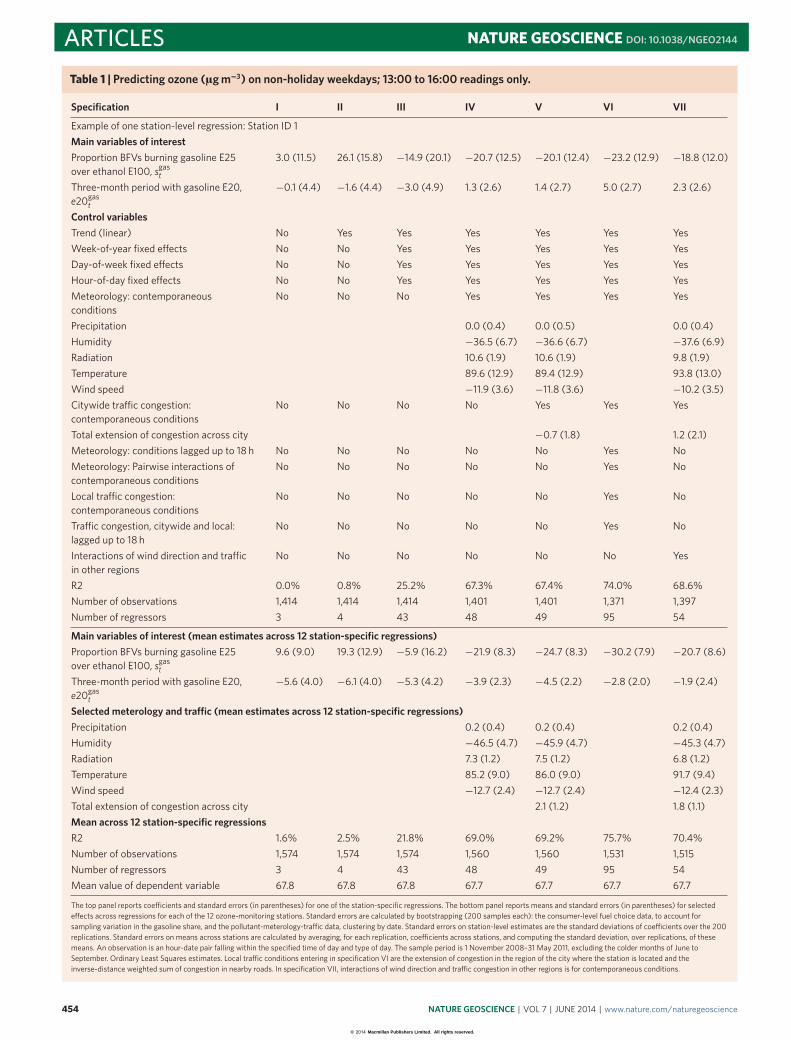
O3 reduction and NO and CO increase with shift to gasolineAcross specifications IV–VII of Table 1, the average fuel mix effectλ1 (see equation (1)) on the ozone concentration is estimated at−20.7 to −30.2 µgm−3, with standard errors on mean (s.e.m.)of under 9 µgm−3. This range of estimates corresponds to astatistically significant reduction in ambient ozone levels, as thegasoline share rose by 62 percentage points, of about 15 µgm−3(λ1 averaged across the columns times 0.62). This 15 µgm−3 dropamounts to 22% of the mean value of the dependent variable—

observed ozone concentrations in the early afternoon on non-holiday weekdays average 68 µgm−3. Figure 4 plots mean changesin ozone concentrations, as the gasoline share rose 62 percentagepoints, estimated not only for the early afternoon but also for othertimes of the day (using specification VI).

We also estimate a mean negative coefficient λ2 on the gasolineE20 blend dummyvariable, e20gast , suggesting thatO3 concentrationswere similarly lower in the three-month period from Februaryto April 2010, during which the gasoline fuel dispensed toconsumers contained five percentage points less ethanol (moregasoline) by volume. This estimated negative effect λ2, however, isonly marginally significant (columns IV and V) to insignificantlydifferent from zero (column VII), probably as a result of thesmaller magnitude of the ethanol–gasoline shift over this episode(Supplementary Information Part F). Nonetheless, that we estimateλ1 and λ2 to be of the same sign—based on continuously valued anddiscretely valued variables, respectively—increases our confidencethat our identifying assumption holds (see equation (2) inMethods)






Table 1 | Predicting ozone (µgm−3) on non-holiday weekdays; 13:00 to 16:00 readings only.

Specification I II III IV V VI VII

Example of one station-level regression: Station ID 1Main variables of interestProportion BFVs burning gasoline E25over ethanol E100, sgas

t

3.0 (11.5) 26.1 (15.8) −14.9 (20.1) −20.7 (12.5) −20.1 (12.4) −23.2 (12.9) −18.8 (12.0)

Three-month period with gasoline E20,e20gas

t

−0.1 (4.4) −1.6 (4.4) −3.0 (4.9) 1.3 (2.6) 1.4 (2.7) 5.0 (2.7) 2.3 (2.6)

Control variablesTrend (linear) No Yes Yes Yes Yes Yes YesWeek-of-year fixed e�ects No No Yes Yes Yes Yes YesDay-of-week fixed e�ects No No Yes Yes Yes Yes YesHour-of-day fixed e�ects No No Yes Yes Yes Yes YesMeteorology: contemporaneousconditions

No No No Yes Yes Yes Yes

Precipitation 0.0 (0.4) 0.0 (0.5) 0.0 (0.4)Humidity −36.5 (6.7) −36.6 (6.7) −37.6 (6.9)Radiation 10.6 (1.9) 10.6 (1.9) 9.8 (1.9)Temperature 89.6 (12.9) 89.4 (12.9) 93.8 (13.0)Wind speed −11.9 (3.6) −11.8 (3.6) −10.2 (3.5)Citywide tra�c congestion:contemporaneous conditions

No No No No Yes Yes Yes

Total extension of congestion across city −0.7 (1.8) 1.2 (2.1)Meteorology: conditions lagged up to 18 h No No No No No Yes NoMeteorology: Pairwise interactions ofcontemporaneous conditions

No No No No No Yes No

Local tra�c congestion:contemporaneous conditions


Tra�c congestion, citywide and local:lagged up to 18 h


Interactions of wind direction and tra�cin other regions

No No No No No No Yes

R2 0.0% 0.8% 25.2% 67.3% 67.4% 74.0% 68.6%Number of observations 1,414 1,414 1,414 1,401 1,401 1,371 1,397Number of regressors 3 4 43 48 49 95 54

Main variables of interest (mean estimates across 12 station-specific regressions)Proportion BFVs burning gasoline E25over ethanol E100, sgas

t

9.6 (9.0) 19.3 (12.9) −5.9 (16.2) −21.9 (8.3) −24.7 (8.3) −30.2 (7.9) −20.7 (8.6)


t

−5.6 (4.0) −6.1 (4.0) −5.3 (4.2) −3.9 (2.3) −4.5 (2.2) −2.8 (2.0) −1.9 (2.4)

Selected meterology and tra�c (mean estimates across 12 station-specific regressions)Precipitation 0.2 (0.4) 0.2 (0.4) 0.2 (0.4)Humidity −46.5 (4.7) −45.9 (4.7) −45.3 (4.7)Radiation 7.3 (1.2) 7.5 (1.2) 6.8 (1.2)Temperature 85.2 (9.0) 86.0 (9.0) 91.7 (9.4)Wind speed −12.7 (2.4) −12.7 (2.4) −12.4 (2.3)Total extension of congestion across city 2.1 (1.2) 1.8 (1.1)Mean across 12 station-specific regressionsR2 1.6% 2.5% 21.8% 69.0% 69.2% 75.7% 70.4%Number of observations 1,574 1,574 1,574 1,560 1,560 1,531 1,515Number of regressors 3 4 43 48 49 95 54Mean value of dependent variable 67.8 67.8 67.8 67.7 67.7 67.7 67.7

The top panel reports coe�cients and standard errors (in parentheses) for one of the station-specific regressions. The bottom panel reports means and standard errors (in parentheses) for selectede�ects across regressions for each of the 12 ozone-monitoring stations. Standard errors are calculated by bootstrapping (200 samples each): the consumer-level fuel choice data, to account forsampling variation in the gasoline share, and the pollutant-meterology-tra�c data, clustering by date. Standard errors on station-level estimates are the standard deviations of coe�cients over the 200replications. Standard errors on means across stations are calculated by averaging, for each replication, coe�cients across stations, and computing the standard deviation, over replications, of thesemeans. An observation is an hour-date pair falling within the specified time of day and type of day. The sample period is 1 November 2008–31 May 2011, excluding the colder months of June toSeptember. Ordinary Least Squares estimates. Local tra�c conditions entering in specification VI are the extension of congestion in the region of the city where the station is located and theinverse-distance weighted sum of congestion in nearby roads. In specification VII, interactions of wind direction and tra�c congestion in other regions is for contemporaneous conditions.






−30

−20

−10

0Ch

ange

in o

zone

conc

entr

atio

n (µ

g m

−3) 01

:00

to 0

6:00

07:0

0 to

10:0

0

10:0

0 to

1 3:0

0

13:0

0 to

16:0

0

17:0

0 to

20:

00

21:0

0 to

00:

00

Day time (h)

0.4

0.2

0.0Chan

ge in

CO

conc

entr

atio

n (p

pm)

40

20

0Chan

ge in

NO

conc

entr

atio

n (µ

g m

−3)

−100

−50

0

Perc

enta

ge o

f cha

nge

in o

zone

con

cent

ratio

n 01:0

0 to

06:

00

07:0

0 to

10:0

0

10:0

0 to

13:0

0

13:0

0 to

16:0

0

17:0

0 to

20:

00

21:0

0 to

00:

00

Day time (h)

100

50

0

150

100

50

0Perc

enta

ge o

f ch a

nge

in N

O c

once

ntra

tion

Perc

enta

ge o

f cha

nge

in C

O c

once

ntra

tion

Figure 4 | Estimated changes in O3, NO, and CO concentrations as the gasoline share, sgast , rose by 62 percentage points. Mean e�ects across regressionsfor the stations monitoring each given pollutant, for di�erent times on a non-holiday weekday. The left panels plot the 95% confidence intervals for (themean across monitors of) 0.62λ1 and the right panels express these confidence intervals as proportions of mean recorded concentrations at the di�erenttimes of a non-holiday weekday. Source: specification VI estimates (Table 1 and Table 2). See the footnote to Table 1 on how the error bars were obtained.

and that the negative coefficient on sgast is not being driven by sometime-varying omitted variable that, after controlling for a lineartrend, still happens to be spuriously correlated with the gasolineshare.We note that our results are very robust to replacing the lineartrend by a quadratic one.

Table 2 presents the same analysis for NO,NO2 and CO, based onconcentrations measured in the morning rush hours (07:00–10:00)of non-holiday weekdays at 9 NOX -monitoring stations and 11 CO-monitoring stations. For brevity, the table reports estimated effectsaveraged across station-specific regressions (individual estimatesare provided in the Supplementary Information).

Point estimates of the effect λ1 of raising the gasoline sharetend to be positive for NO and for CO, but these effects are lessprecisely estimated than for O3. As with O3, the estimated effectλ2 of the step change in the gasoline blend is of the same sign asλ1. Averaging across specifications IV–VII, a 62-percentage-pointrise in the gasoline share is associated with increases of 17.3 µgm−3(s.e.m. 7.6 µgm−3) and 0.22 ppm (s.e.m. 0.07 ppm) in ambient NOand CO concentrations, respectively—amounting to 26 and 18% ofthe mean readings during morning rush hours (also see Fig. 4 forother times of the day). Finally, the estimated effect λ1 for NO2 isnot significantly different from zero—point estimates are smallerand noisier than those for NO, whose ambient concentrations arearound 40% higher compared with NO2.

Figure 3c,d offers an intuitive illustration of our method and ofour result for ozone. Figure 3c plots O3 concentrations measuredin the early afternoon hours on non-holiday weekdays against thegasoline share sgast . There happens to be a positive relationshipin the raw data (only to illustrate, here we pool observationsat all O3 monitors). The vertical axis in Fig. 3d shows fittedresiduals of a regression of O3 concentrations on all independentvariables except sgast (we use specification VI plus monitor fixed

effects for this pooled regression). These residual concentrationsare the variation in ozone that is left unexplained once variation inmeteorology, traffic, seasonality, trending omitted factors, and thegasoline blend change are accounted for. The horizontal axis plotsresiduals from a regression of sgast on the same vector of independentvariables: these share residuals capture the component of variationin the gasoline-over-ethanol consumer choice that is orthogonalto the other regressors. The relationship between the residual O3concentrations and the residual gasoline share is negative, with a λ1slope of −31.6 µgm−3; this is similar to the mean coefficient acrossstation-specific regressions in column VI, Table 1.

In Supplementary Information Part F we perform a placebo testand subject our baseline results to a number of extra robustnesschecks, including: specifying dependent variables as logarithmictransforms of the units of measurement; keeping the colder monthsof June to September in the sample; controlling for recorded trafficspeeds on top of congestion; controlling for the real price of diesel,monthly ridership on the public transport system, monthly physicalindustrial production for the state of São Paulo, and employmentor wages in the metropolis. We also note that gone are the daysin which the city of São Paulo was an industrial hub, and thatnow the electricity that serves southeastern Brazil is predominantlygenerated by hydropower. In sum, factors that might otherwiseconfound identification of the effect of the fuel mix on air qualityare less of a concern in the present study.

Towards quantitative benchmarks for model studiesOur results stand at variance to those of the recent computersimulation that was calibrated to the São Paulo system25 whichpredicted large reductions in ozone concentrations from ahypothetical switch to ethanol that—although larger than the onewe observe in the data—is of comparable magnitude. Our joint data






Table 2 | Predicting NO (µgm−3), NO2 (µgm−3), and CO (ppm) on non-holiday weekdays; 07:00–10:00 readings only.

Specification I II III IV V VI VII

Dependent variable: NO concentration (µgm−3)Main variables of interest (mean estimates across 9 station-specific regressions)Proportion BFVs burning gasoline E25over ethanol E100, sgas

t

−17.4 (12.6) 3.6 (19.7) 45.6 (21.1) 29.2 (12.2) 28.2 (12.3) 22.7 (12.4) 31.7 (11.9)


t

6.7 (4.5) 6.1 (4.5) 8.3 (5.5) 11.8 (3.8) 11.8 (3.8) 9.7 (4.0) 11.0 (3.9)

Selected meterology and tra�c (mean estimates across 9 station-specific stations)Precipitation −0.4 (0.4) −0.4 (0.5) −0.5 (0.5)Humidity −19.6 (11.6) −19.7 (11.7) −18.1 (11.0)Radiation 3.5 (1.1) 3.6 (1.1) 3.5 (1.1)Temperature −17.0 (13.8) −17.0 (13.8) −25.7 (13.8)Wind speed −52.3 (3.2) −52.3 (3.2) −51.2 (3.2)Total extension of congestion across city 1.4 (2.9) 1.8 (2.9)Mean across 9 station-specific regressionsR2 0.9% 1.5% 21.0% 43.2% 43.3% 53.2% 45.9%Number of observations 1,529 1,529 1,529 1,514 1,514 1,489 1,464Number of regressors 3 4 43 48 49 95 54Mean value of dependent variable 66.5 66.5 66.5 66.5 66.5 67.0 66.8

Dependent variable: NO2 concentration (µgm−3)Main variables of interest (mean estimates across 9 station-specific regressions)Proportion BFVs burning gasoline E25over ethanol E100, sgas

t

−4.4 (3.6) −2.6 (5.0) 5.0 (6.4) −5.3 (4.7) −6.2 (4.7) 5.1 (4.4) −5.8 (4.8)


t

3.3 (1.7) 3.3 (1.7) 3.7 (1.9) 4.6 (1.3) 4.5 (1.3) −0.7 (1.2) 4.5 (1.4)

Selected meterology and tra�c (mean estimates across 9 station-specific stations)Precipitation 0.3 (0.2) 0.3 (0.2) 0.2 (0.2)Humidity −28.2 (4.7) −28.3 (4.7) −26.7 (4.7)Radiation 1.3 (0.5) 1.3 (0.5) 1.4 (0.5)Temperature 33.6 (4.7) 33.6 (4.8) 31.2 (4.8)Wind speed −10.4 (0.8) −10.4 (0.8) −9.9 (0.8)Total extension of congestion across city 1.1 (1.0) 1.0 (1.0)Mean across station specific regressionsR2 2.9% 4.7% 21.9% 40.3% 40.4% 58.4% 42.9%Number of observations 1,529 1,529 1,529 1,514 1,514 1,489 1,464Number of regressors 3 4 43 48 49 95 54Mean value of dependent variable 48.1 48.1 48.1 48.0 48.0 48.1 47.9

Dependent variable: CO concentration (ppm)Main variables of interest (mean estimates across 11 station-specific regressions)Proportion BFVs burning gasoline E25over ethanol E100, sgas

t

0.15 (0.13) 0.35 (0.21) 0.66 (0.22) 0.34 (0.12) 0.33 (0.12) 0.41 (0.11) 0.34 (0.12)


t

0.08 (0.05) 0.07 (0.05) 0.10 (0.06) 0.17 (0.04) 0.17 (0.04) 0.11 (0.04) 0.16 (0.04)

Selected meterology and tra�c (mean estimates across 11 station-specific stations)Precipitation 0.00 (0.01) 0.00 (0.01) 0.0 (0.01)Humidity 0.16 (0.12) 0.16 (0.12) 0.20 (0.12)Radiation 0.06 (0.01) 0.06 (0.01) 0.06 (0.01)Temperature 0.70 (0.14) 0.70 (0.14) 0.63 (0.14)Wind speed −0.49 (0.03) −0.49 (0.03) −0.48 (0.03)Total extension of congestion across city 0.01 (0.03) 0.01 (0.03)Mean across 11 station-specific regressionsR2 1.2% 2.0% 24.6% 48.9% 49.0% 59.8% 51.5%Number of observations 1,565 1,565 1,565 1,548 1,548 1,523 1,505Number of regressors 3 4 43 48 49 95 54Mean value of dependent variable 1.20 1.20 1.20 1.20 1.20 1.20 1.20

See footnote to Table 1. Estimated mean coe�cients and standard errors on means (in parentheses) across station-specific regressions (9 stations monitoring nitrogen oxides and 11 stations monitoringCO). Standard errors account for estimation of the gasoline share.





NATURE GEOSCIENCE DOI: 10.1038/NGEO2144 ARTICLESanalysis of pollutant concentrations, meteorological and road trafficconditions, and consumer fuel choice indicates that early-afternoonO3 concentrations declined by an average 15 µgm−3 (22% of thesample mean) as the share of bi-fuel vehicles burning gasolinegrew from 14 to 76%. Such empirical findings are consistent withthe modelling hypothesis that O3 production over the São Paulometropolis may be hydrocarbon-limited39, whereby higher NOXemissions (from gasoline) would result in reductions in ambientozone. Hydrocarbon-limited O3 production would also rationalizewhy O3 levels tend to increase, and NOX and CO levels tend todecrease, on weekends, when road traffic congestion falls. Suchan interpretation for our São Paulo result should be contrastedwith the claim that ‘(m)easurements and model calculationsnow show that O3 production over most of the United Statesis primarily NOX -limited, not hydocarbon-limited’31. Clearly,successful strategies against ozone pollution require knowledgeof the local regime. Moreover, with access to the relevant air (andother) monitoring data for the area outside of the heavily urbanizedSão Paulo metropolis, our approach is potentially applicable for theestimation of ozone and NOX concentrations in suburban or ruralareas downwind.

Our present study has shown that under atmospheric conditionsobserved in São Paulo, concentrations of two air pollutants,specifically NO and CO, may increase whereas that of ozone falls onraising the gasoline fuel share. We caution that the concentrationof particles, specifically fine particulate matter, may also increaseunder that situation. Given that the method presented here allows,in principle, for the evaluation of how different fuel mixes impactpollutants other than ozone and NOX , such as particulate matter, itis our view that studies such as ours may help inform scientists andpolicymakers alike on the benefits and disadvantages that certainfuel mixes may have on ambient levels of pollutants, be they in thegas or condensed phase.

MethodsNot unlike the ‘chemical coordinates’ approach put forth by Cohen et al.40, weapply a multivariate regression analysis of a real-world dataset exhibiting, in thepresent case, rich and exogenous time variation in fuel mix41. The idea is tocompare pollutant concentrations across subsamples which differ only in the fuelmix—gasoline versus ethanol—but are otherwise similar with regard to otherdeterminants of air quality, including meteorology, anthropogenic activity, andbiogenic activity. We directly control for variation in local meteorological andvehicle traffic conditions, contemporaneously and in the several hours thatprecede an observation. Our regressions flexibly predict a pollutant’sconcentration specific to the location of the air monitor and time and type of day,using a relatively short sample period during which the fuel mix varied, namelylate 2008 to mid 2011. We drop the colder months from June to Septemberfrom the baseline sample. We thus control for unobserved variation thatmight potentially confound our inference of the effect of the fuel mix onair quality.

Our baseline regression equation, which we estimate separately by location ofmeasurement and time and type of day, takes the following form:

concentrationt=λ1sgast +λ2e20

gast +W ′

t1W+T ′t1

T+ fixedeffectst+ trendt+εt (1)

An observation t is an hour–date pair, for example, for the Diadema station, earlyafternoon (13:00–16:00), non-holiday weekday regression, an observation is 14:00on Monday 14 March 2011 (this was not a public holiday). The dependentvariable concentrationt corresponds to a pollutant that is measured at the station,for example, O3, in the measured units (µgm−3) or a logarithmic transformthereof. Both fuel mix variables, sgast and e20gast , increase in the proportion ofgasoline, although the shift from ethanol to gasoline as e20gast changes from 0 to 1is of lesser magnitude—we thus expect the effect λ2 to have a lower magnitudethan, but exhibit the same sign as, λ1. Wt and Tt are vectors of contemporaneousand lagged meteorological and traffic controls that are local to the particularstation of measurement, as detailed in the Supplementary Information, and 1W

and 1T are coefficients. To account for seasonal variation, we include full sets ofweek-of-year, day-of-week, and hour-of-day fixed effects; for the Diadema stationobservation in the example, the week 11 (14 March 2011), Monday, and 14:00indicators would be on. We also allow for a linear or quadratic trend in the dateto control for potentially confounding omitted time-varying factors. The

identifying assumption is that, conditional on controls, the residual isuncorrelated with the fuel mix, in particular:

E[sgast εt |Xt ]=0, where Xt :=(Wt ,Tt , fixedeffectst , trendt ) (2)

A concern that might arise in a real-world—as opposed to lab orsynthetic—setting such as ours is the possibility that consumers may have cutback on vehicle usage when faced with rising ethanol prices. If this were the case,not controlling for vehicle usage would confound our estimation of the effect ofvarying the fuel mix on air quality, as the corresponding orthogonality condition(without covariates Tt ) would not hold. Two points should be noted. First, we doadd detailed controls for local and citywide road traffic congestion and speedrecorded at the hourly level. Second, we show that traffic conditions and thusvehicle usage, although predictable, did not significantly vary with fuel pricesduring the sample period. This finding can be rationalized on different counts,namely: the typically price-inelastic short-run demand for vehicle usage due tothe poor availability of substitutes42, including public transportation, as evidencedby ridership records (Supplementary Information Part E); the existence of‘repressed demand’ for vehicle usage that has been argued in the face ofwidespread gridlock43,44; and the relatively subdued variation in the price ofgasoline—which can fuel nine-tenths of São Paulo’s light-duty fleet of bi-fuel andsingle-fuel vehicles.

With regard to the gasoline share among bi-fuel consumers sgast , oneapproach45 would be to assume that consumers perceive gasoline and ethanol tobe ‘perfect substitutes’, thus fuelling their bi-fuel vehicles with the fuel that yieldsthe lowest $ per distance travelled. By this assumption, consumers would switchfrom ethanol to gasoline, sgast =1, whenever the per-litre price of ethanolsurpassed around 70% of the per-litre price of gasoline, and sgast would be 0otherwise. The analysis could then follow a regression discontinuity design46.However, surveys of Brazilian motorists making choices at the pump have shownthat there is substantial heterogeneity in consumer behaviour and that, ratherthan discontinuously, fuel switching occurs gradually over a wide range of relativeprice variation12. Our measure of sgast , which ranges from 14 to 76% in-sample, isobtained from an estimated consumer demand system, based on the multinomialprobit model47. For robustness, we obtain a similar gasoline share on estimatingan alternative consumer-level choice model based on the multinomial logit.Figure 3 reports how the gasoline share, sgast , varies in the sample: (Fig. 3a) withthe per-litre ethanol-to-gasoline price ratio—notice that there is no kink at theapproximate 70% ‘parity’ threshold, at which $/mile travelled on either fuel isabout the same; and (Fig. 3b) over time (see Supplementary Information Part Afor demand modelling and estimation). The data archive can be accessed athttp://bit.do/salvo_geiger_data.

Received 2 October 2013; accepted 18 March 2014;published online 28 April 2014

References1. Martins, L. & Andrade, M. Ozone formation potentials of volatile organic

compounds and ozone sensitivity to their emission in the megacity of SãoPaulo, Brazil.Water Air Soil Poll. 195, 201–213 (2008).

2. CETESB, Relatório Anual sobre a Qualidade do Ar no Estado de São Paulo[Annual Report on Air Quality in the State of São Paulo] (CompanhiaAmbiental do Estado de São Paulo, 2010).

3. La Rovere, E. L. Inventário de Emissões de Gases de Efeito Estufa do Município deSão Paulo [Greenhouse Gas Emissions Inventory for the Municipality of SãoPaulo] (Centro de Estudos Integrados sobre Meio Ambiente e MudançasClimáticas, Universidade Federal do Rio de Janeiro, 2005).

4. Fann, N. et al. Estimating the national public health burden associated withexposure to ambient PM2.5 and ozone. Risk Anal. 32, 81–95 (2012).

5. Gauderman, W. J. et al. Effect of exposure to traffic on lung development from10 to 18 years of age: A cohort study. Lancet 369, 571–577 (2007).

6. Ponce, N. A., Hoggatt, K. J., Wilhelm, M. & Ritz, B. Preterm birth: Theinteraction of traffic-related air pollution with economic hardship in LosAngeles neighborhoods. Am. J. Epid. 162, 140–148 (2005).

7. Currie, J. & Walker, R. Traffic congestion and infant health: Evidence fromE-ZPass. Am. Econ. J.-Appl. Econ. 3, 65–90 (2011).

8. Salvo, A. & Huse, C. Is arbitrage tying the price of ethanol to that of gasoline?Evidence from the uptake of flexible-fuel technology. Energy J. 32,119–148 (2010).

9. Goldemberg, J. Ethanol for a sustainable energy future. Science 315,808–810 (2007).

10. http://www.anp.gov.br/preco/prc/Resumo_Por_Municipio_Index.asp11. http://www.anp.gov.br/?dw=1103112. Salvo, A. & Huse, C. Build it, but will they come? Evidence from consumer

choice between gasoline and sugarcane ethanol. J. Environ. Econ. Manag.251–279 (2013).




http://bit.do/salvo_geiger_data

http://www.anp.gov.br/preco/prc/Resumo_Por_Municipio_Index.asp

http://www.anp.gov.br/?dw=11031



13. Al-Hasan, M. Effect of ethanol-unleaded gasoline blends on engineperformance and exhaust emission. Energy Convers. Manag. 44,1547–1561 (2003).

14. Graham, L. A., Belisle, S. L. & Baas, C-L. Emissions from light duty gasolinevehicles operating on low blend ethanol gasoline and E85. Atmos. Environ. 42,4498–4516 (2008).

15. He, B-Q., Jian-Xin, W., Hao, J-M., Yan, X-G. & Xiao, J-H. A study on emissioncharacteristics of an EFI engine with ethanol blended gasoline fuels. Atmos.Environ. 37, 949–957 (2003).

16. Hsieh, W-D., Chen, R-H., Wu, T-L. & Lin, T-H. Engine performance andpollutant emission of an SI engine using ethanol-gasoline blended fuels. Atmos.Environ. 36, 403–410 (2002).

17. Jia, L-W., Shen, M-Q., Wang, J. & Lin, M-Q. Influence of ethanol–gasolineblended fuel on emission characteristics from a four-stroke motorcycle engine.J. Haz. Mat. 123, 29–34 (2005).

18. Leong, S. T., Muttamara, S. & Laortanakul, P. Applicability of gasolinecontaining ethanol as Thailand’s alternative fuel to curb toxic VOC pollutantsfrom automobile emission. Atmos. Environ. 36, 3495–3503 (2002).

19. Lynd, L. R. Overview and evaluation of fuel ethanol from cellulosic biomass:Technology, economics, the environment, and policy. Ann. Rev. EnergyEnviron. 21, 403–465 (1996).

20. Mulawa, P. A. et al. Effect of ambient temperature and E-10 fuel on primaryexhaust particulate matter emissions from light-duty vehicles. Environ. Sci.Technol. 31, 1302–1307 (1997).

21. Poulopoulos, S. G., Samaras, D. P. & Philippopoulos, C. J. Regulated andunregulated emissions from an internal combustion engine operating onethanol-containing fuels. Atmos. Environ. 35, 4399–4406 (2001).

22. Topgül, T., Yücesu, H. S., Çinar, C. & Koca, A. The effects of ethanol–unleadedgasoline blends and ignition timing on engine performance and exhaustemissions. Renew. Energy 31, 2534–2542 (2006).

23. Yoon, S. H., Ha, S. Y., Roh, H. G. & Lee, C. S. Effect of bioethanol as analternative fuel on the emissions reduction characteristics and combustionstability in a spark ignition engine. J. Auto Engin. 223, 941–951 (2009).

24. Pereira, P. A. d. P., Santos, L. M. B., Sousa, E. T. & Andrade, J. B. d. Alcohol- andgasohol-fuels: a comparative chamber study of photochemical ozoneformation. J. Braz. Chem. Soc. 15, 646–651 (2004).

25. Martins, L. D. & Andrade, M. F. Emission scenario assessment of gasoholreformulation proposals and ethanol use in the metropolitan area of São Paulo.Open Atmos. Sci. J. 2, 166–175 (2008).

26. Ginnebaugh, D. L., Liang, J. & Jacobson, M. Z. Examining the temperaturedependence of ethanol (E85) versus gasoline emissions on air pollution with alargely-explicit chemical mechanism. Atmos. Environ. 44, 1192–1199 (2010).

27. Jacobson, M. Z. Effects of ethanol (E85 versus gasoline vehicles on cancer andmortality in the United States. Environ. Sci. Technol. 41, 4150–4157 (2007).

28. Beer, T. et al. The health impacts of ethanol blend petrol. Energies 4,352–367 (2011).

29. Finlayson-Pitts, B. & Pitts, J. Chemistry of the Upper and Lower Atmosphere:Theory, Experiments, and Applications (Academic Press, 2000).

30. Seinfeld, J. H. & Pandis, S. N Atmospheric Chemistry and Physics: From AirPollution to Climate Change (Wiley, 1998).

31. Jacob, D. J. Introduction to Atmospheric Chemistry (Princeton Univ. Press,1999).

32. Anderson, L. G. Ethanol fuel use in Brazil: Air quality impacts. Energy Environ.Sci. 2, 1015–1037 (2009).

33. Romieu, I., Weitzenfeld, H. & Finkelman, J. Urban air pollution in LatinAmerica and the Caribbean. J. Air Waste Manag. 41, 1166–1171 (1991).

34. US Senate Hearing 106-953 (US Government Printing Office, 2000).35. US Senate Hearing 109-857 (Presentation by Mr Eduardo Pereira de Carvalho,

president of UNICA, downloaded on November 17 2011 from website of Office ofUS Senator Richard G. Lugar)(US Government Printing Office, 2006).

36. http://cbn.globoradio.globo.com/home/HOME.htm37. http://www.inmet.gov.br/38. http://cetsp1.cetsp.com.br/monitransmapa/agora/39. Orlando, J. P., Alvim, D. S., Yamazaki, A., Corrêa, S. M. & Gatti, L. V. Ozone

precursors for the São Paulo metropolitan area. Sci. Tot. Environ. 408,1612–1620 (2010).

40. Cohen, R. C. et al. Quantitative constraints on the atmospheric chemistry ofnitrogen oxides: An analysis along chemical coordinates. J. Geophys. Res.:Atmos. 105, 24283–24304 (2000).

41. Auffhammer, M. & Kellogg, R. Clearing the air? The effects of gasoline contentregulation on air quality. Am. Econ. Rev. 101, 2687–2722 (2011).

42. Hughes, J. E., Knittel, C. R. & Sperling, D. Evidence of a shift in the short-runprice elasticity of gasoline demand. Energy J. 29, 113–134 (2008).

43. Duranton, G. & Turner, M. A. The fundamental law of road congestion:Evidence from US cities. Am. Econ. Rev. 101, 2616–2652 (2011).

44. Vickrey, W. S. Congestion theory and transport investment. Am. Econ. Rev. 59,251–260 (1969).

45. Holland, S. P., Hughes, J. E. & Knittel, C. R. Greenhouse gas reductions underlow carbon fuel standards? Am. Econ. J.-Econ. Polic. 1, 106–146 (2009).

46. Bento, A., Kaffine, D., Roth, K. & Zaragoza-Watkins, M. The effects ofregulation in the presence of multiple unpriced externalities: Evidence from thetransportation sector. Am. Econ. J.-Econ. Polic. (in the press).

47. Goolsbee, A. & Petrin, A. The consumer gains from direct broadcast satellitesand the competition with cable TV. Econometrica 72, 351–381 (2004).

AcknowledgementsWe gratefully acknowledge numerous people from CETESB, INMET, CET and ANP forgenerously sharing their data; CBN Notícias for sharing their newscasts; and Raízen forsharing access to their fuelling stations. In particular, we thank W. Baptista, C. Costa, A.Dall’Antonia Jr, F. Henkes, M. Kuromoto, C. Lacava, D.G. Medeiros, R.C. Melo, R. dosSantos and T. P. Senaubar. We thank T. Aguirre for summarizing descriptive CETESB andCPTEC weather reports, M. Peterson for preparing a literature review as well as an initialwritten and graphical description of the pollutant and meteorological data, and S. Ritcheyfor listing the GPS coordinates of road segments. We thank S. Budanova, E. Lehman andC. Maalouf for research assistance, as well as J. Brito, M. Busse, J. He, E. Mansur and S.McRae for helpful comments. A.S. acknowledges support from the Initiative forSustainability and Energy at Northwestern University (ISEN) and from the Dean’s Officeat the Kellogg School of Management, Northwestern University. F.M.G. thanks the NSFAtmospheric and Geospace Science division for support under grant # NSFATM-0533436 and gratefully acknowledges support from an Irving M. Klotzprofessorship in physical chemistry.

Author contributionsA.S. conceived the research; A.S. and F.M.G. analysed the data and wrote the paper.

Additional informationSupplementary information is available in the online version of the paper. Reprints andpermissions information is available online at www.nature.com/reprints.Correspondence and requests for materials should be addressed to A.S.

Competing financial interestsThe authors declare no competing financial interests.




http://cbn.globoradio.globo.com/home/HOME.htm

http://www.inmet.gov.br/

http://cetsp1.cetsp.com.br/monitransmapa/agora/


http://www.nature.com/reprints


ozone nature

Environment

ethanol use

ethanol emissions

gasoline emissions

ethanol e100

total gasoline

price of ethanol relative

relative price of ethanol

gasolinebased vehicles