oulu business school - search homejultika.oulu.fi/files/nbnfioulu-201401171043.pdf · university of...
TRANSCRIPT
OULU BUSINESS SCHOOL
Juho Isola
DISENTANGLING HIGH-FREQUENCY TRADERS’ ROLE IN ETF MISPRICING
Master’s Thesis
Department of Finance
December 2013

UNIVERSITY OF OULU ABSTRACT OF THE MASTER'S THESIS
Oulu Business School
Unit
Department of Finance Author
Isola Juho Supervisor
Kahra H. Professor Title
Disentangling High-Frequency Traders’ Role in ETF Mispricing Subject
Finance Type of the degree
M.Sc thesis Time of publication
December 2013 Number of pages
71 Abstract
Exchange Traded Funds (ETFs) should trade at a price equal to their fundamental Net Asset Value
(NAV). However, ETFs’ can occasionally pose economically significant premiums/discounts to their
NAV prices, i.e. arbitrage opportunities. The theoretical part focuses on ETF arbitrage and explains
why this arbitrage trading is attractive to high-frequency traders (HFTs).
In the empirical part, we introduce HFT activity proxies to a factor model explaining the observed
SPDR trust (SPY) premiums during 2.1.2002–15.1.2013. A range of statistical and econometrical
tools are then employed to study the detailed relationship between these factors and the SPY premi-
ums. In addition, we replicate a popular method used to study HFTs’ effects on stock markets, and
apply it to analyze HFTs’ effects on ETF pricing process. By utilizing an exogenous technology shock
(implementation of Regulation National Market System) which improved U.S. market infrastructure,
we should be able to dissect the effects caused by heightened HFT activity.
The absolute size of SPY premium is significantly related to endogenous ETF factors. The exogenous
factors serving as proxies for available arbitrage capital improve the explanatory power. The Reg.
NMS implementation fails to serve as an exhaustive structural break point in ETF pricing dynamics.
Although, the post-Reg. NMS era has very low ETF premiums and higher trading volumes. This can
indicate that Reg. NMS made markets more suitable for HFT, and therefore high-frequency ETF arbi-
trage might have been more efficient during the post-Reg. NMS era.
Simple implications are: ETF premiums can be significant in relation to their annual expense ratios
and investors can improve their trade execution by understanding the drivers behind ETF premiums.
ETF premium volatility modeling can also be useful in risk management and in investment decision
making. Understanding HFTs’ role in ETF mispricing adds to our incomplete knowledge on the ef-
fects of individual HFT strategies.
Keywords
Volatility modeling, ETF arbitrage, Regulation NMS, Time-varying beta estimation Additional information
CONTENTS
1 INTRODUCTION............................................................................................................ 5
2 TERMINOLOGY ............................................................................................................ 8
2.1 Algorithmic trading ................................................................................................. 8
2.2 High-frequency trading ............................................................................................ 8
2.3 Exchange-traded funds ............................................................................................ 9
2.4 ETF arbitrage ......................................................................................................... 11
3 PRIOR LITERATURE .................................................................................................. 12
4 THE NATURE OF HIGH-FREQUENCY TRADING .................................................. 16
4.1 A brief history ........................................................................................................ 16
4.2 HFT strategies ........................................................................................................ 17
4.3 How to spot a player? ............................................................................................ 19
4.4 A new normal in risk management ........................................................................ 21
5 THEORETICAL FRAMEWORK ................................................................................. 23
5.1 Arbitrage in financial markets ............................................................................... 23
5.2 Understanding ETF arbitrage at high-frequency ................................................... 24
6 RESEARCH DESIGN AND RESEARCH QUESTIONS ............................................. 27
6.1 Research problems and methodology .................................................................... 27
6.2 Research questions and objective .......................................................................... 30
7 RESEARCH DATA ....................................................................................................... 31
7.1 Data description and sources ................................................................................. 31
7.2 Descriptive statistics .............................................................................................. 32
8 EMPIRICAL RESULTS ................................................................................................ 36
8.1 The factors behind ETF premiums ........................................................................ 36
8.2 ETF premium dynamics prior and after Reg. NMS ............................................... 39
8.3 ETF premium volatility modeling ......................................................................... 47
9 SUMMARY ................................................................................................................... 50
10 DISCUSSION ................................................................................................................ 52
REFERENCES ...................................................................................................................... 54
APPENDICES
Appendix I List of factors and data sources ................................................................ 62
Appendix II Correlations between independent variables. .......................................... 65
Appendix III Figures of SPY time-series .................................................................... 66
Appendix IV Regression results prior and after Reg. NMS ........................................ 67
Appendix V Figures of rolling regression coefficients ................................................ 68

FIGURES
Figure 1. Rolling regression coefficients using TED and SPY_VOL ........................................... 43
Figure 2. The time-varying betas using Kalman filters for TED and SPY_VOL as the independent
variables and abs(ETF premium) as the dependent variable ......................................................... 45
Figure 3. Recursive CUSUM test .................................................................................................. 46
Figure 4. Fitted SPY premium volatility time-series 09.07.2007 – 22.09.2011 ............................ 48
Figure 5. SPY premium time-series predictions 23.09.2011 – 31.10.2013 ................................... 49
Figure 6. Rolling SPY premium volatility predictions 23.09.2011 – 31.10.2013 ......................... 49
TABLES
Table 1. Characteristics of HFT (Gomber et al. 2011) .................................................................. 18
Table 2. Classification of high-frequency strategies (Aldridge 2010: 4) ...................................... 18
Table 3. Descriptive statistics of daily ETF mispricing, mean of the absolute size of ETF
mispricing, and annualized premium volatility ............................................................................. 33
Table 4. Correlations between the statistically significant factors behind the absolute size of ETF
premium. Time period 2.1.2002-15.1.2013................................................................................... 33
Table 5. Regression results using daily data and actual level of ETF premium as the dependent
variable .......................................................................................................................................... 36
Table 6. Regression results using daily data and the absolute daily size of ETF premium as the
dependent variable ........................................................................................................................ 38
Table 7. Regression results using rolling 5-day averages ............................................................. 39
Table 8. Regression results prior and after Reg. NMS using the absolute daily size of ETF
premium as the dependent variable ............................................................................................... 41
Table 9. The Chow test F-statistics using daily data and the most statistically and economically
relevant factors .............................................................................................................................. 42
Table 10. GARCH(1,1) model results ........................................................................................... 48

5
1 INTRODUCTION
High-frequency trading has recently been in the spotlight. Contemporary economical
publications and business media publish articles considering the effects of this new
trading norm on a weekly basis1. HFT
2 refers to the use of fast computer-driven op-
erations for trading purposes. Several researchers agree that the recent attention to-
wards HFT partly stems from the events of May 6, 2010 (e.g. Brogaard 2010; Easley
et al. 2011; Gomber et al. 2011; Kirilenko et al. 2011). On that day, the Dow Jones
Industrial Average fell within minutes about 1 000 points (-9.2 %) and then gained
most of those losses immediately. The event has been named as the Flash Crash re-
ferring to its rapid and irregular structure. Many HFT related incidents has followed
since: including single stock Micro Crashes (see Golub et al. 2012; Nanex 2012), the
Shanghai Flash Spike (see Bloomberg 2013; Noble 2013), and malfunctioning algo-
rithms (see Philips 2012).
These market problems are connected to HFTs and algorithms behind the trade or-
ders. The latter refers to algorithmic trading (henceforth AT), a trading method
where orders are conducted through complex mathematical algorithms without hu-
man intervention (see Chaboud et al. 2009; Hendershott & Riordan 2011). The Flash
Crash also drew the regulators’ interest to investigate the role of HFT during the
Flash Crash. However, the following report on the subject does not find HFT as the
direct cause of the event (CFTC-SEC 2010). Kirilenko et al. (2011) note that while
HFTs cannot be blamed for the Flash Crash their behavior might have built up the
volume of the incident. Interestingly, these papers relate exchange-traded funds
(ETFs) and their pricing procedure to problems faced during times of market uncer-
tainty. CFTC-SEC (2010) finds that HFT activity increased over 250 % in NYSE
Arca, the main exchange for ETFs, during a three minute period of the Flash Crash.
This trading activity was higher than the trading in corporate stocks at the same time.
1For concrete examples, see the following international articles (Creswell 2010; Krudy 2010; The
Economist 2013a) and the corresponding Finnish one (Saario 2011). 2Through the study, the abbreviation HFT is used for both high-frequency trading and high-frequency
traders.
6
As has been stressed in various studies, the whole variety of HFT should not be con-
sidered as a single trading strategy, but a tool to implement existing strategies (e.g.
AFM 2010; Gomber et al. 2011; Hagströmer & Nordén 2013). Therefore, in order to
address HFT activity and its relation to systemic risk, market quality measures, and
its future direction we should investigate the individual trading strategies which op-
erate at higher frequency, such as the ETF arbitrage (see Ben-David et al. 2012;
Benos & Sagade 2012). This is clearly a sufficient reason to examine HFT in a de-
tailed manner. The overall social value behind increased trading speed and high-
frequency data analysis has also been questioned (Sornette & von der Becke 2011;
Riordan & Storkenmaier 2012).
This paper examines the relationship between a well-known trading strategy called
the ETF arbitrage and HFT. Previous research and their findings are used to form the
rationale behind the research design: research methods and chosen factors behind
ETF mispricing are partly inspired by prior HFT and ETF studies. We aim to con-
tribute more in connecting HFT activity to ETF pricing process by demonstrating
HFTs’ role in arbitrage activity. This is done by adding some HFT activity proxies to
a simple factor model. The purpose is to address HFTs’ role in ETF mispricing in a
detailed manner and formally test3 if the noted change in ETF mispricing trend is
connected to the rise of HFT. Additional robustness and accuracy examination in-
cludes rolling regression analysis and estimating time-varying factor betas with
Kalman filter method. Finally, the proposed time-series model for ETF mispricing
volatility aims to update premium volatility modeling to incorporate the modern
changes in ETF mispricing trend.
Regression analysis reveals that the absolute size of ETF premium is significantly
related to endogenous ETF factors. In addition, the exogenous factors serving as
proxies for available arbitrage capital improve the explanatory power. The Chow test
proposes that the implementation date of Reg. NMS, which was used as a measure-
ment point for heightened HFT activity, might provide only one possible structural
3This is tested using the Chow Test for structural breaks. The Chow Test is a statistical and economet-
ric test to see if the regression coefficients on different data sets can be considered equal (see Chow
1960).
7
break for the time-series evolution of the ETF premium. Further analysis shows that
the significant regression coefficients and explanatory power behind used factors are
mainly due to the observations during the financial crisis. This analysis also reveals
that the only factors whose relationship with ETF premiums are somewhat persistent
are TED spread and feature scaled ETF trading volume. TED spread shows it signifi-
cance predicting ETF premiums during times of high market stress while ETF trad-
ing volume might serve as a naive factor for heightened HFT activity which is
shrinking ETF premiums via arbitrage activity.
The era of heightened HFT activity has characteristically lower ETF premiums and
the starting point of such an era coincides with the observed changes in the relation-
ships between the significant factors and ETF premiums. However, the statistical
significance cannot be verified using the 95 % confidence intervals in the fluctuation
process of recursive residuals. The proposed simple GARCH(1,1) model with exog-
enous forecasting variables is able to produce satisfactory predictions for the ETF
premium volatility time-series.
The rest of the paper is structured as follows: Section 2 introduces the basic termi-
nology and related concepts needed to understand the research topic more broadly.
Section 3 introduces previous research while section 4 gives more detailed infor-
mation about the nature of HFT, including HFT strategies, difficulties in academic
research, and possible consequences HFT might impose to modern risk management.
Section 5 introduces theoretical aspects of arbitrage activity and connects HFT to
ETF arbitrage. In the main body of this paper, covering sections 6 to 8, research de-
sign, methods, and research questions are explained (6), followed by data sources,
introduction to data sample, and descriptive statistics (7), finally, empirical results
are presented (8). The following section (9) briefly summarizes and the last section
(10) concludes.
As this thesis is a continuum to author’s earlier seminar work, particular sections are
to some extent replicated from the previous work. This mainly concerns terminology
and literature reviews.

8
2 TERMINOLOGY
2.1 Algorithmic trading
Algorithmic trading (AT) is a form of trading where the orders are conducted
through complex mathematical algorithms. Computers using algorithms can create
orders independently. This has reduced trading costs as trading can go on without
human intermediates. Wide range of algorithms are used: some are focusing on find-
ing arbitrage opportunities, some are trying to close large orders at the lowest cost
possible, and some are made to trade on longer-term strategies (Chaboud et al. 2009;
Gomber et al. 2011). Commonly algorithms decide the timing, price level, quantity
and order routing by monitoring markets (Hendershott et al. 2011). AT is often used
by large buy-side traders to group large orders into smaller chunks to manage market
impacts and risks (Fabozzi et al. 2007; Hendershott & Riordan 2011).
2.2 High-frequency trading
High-frequency trading (HFT) refers to the use of rapid computer-driven operations
for trading in financial markets4. The aim is to use large trade volumes to accumulate
the small profits earned per trade (Zhang 2010). Commodity Futures Trading Com-
mission and Securities and Exchange Commission (CFTC-SEC 2010: 45) jointly
define HFT in the following manner: “…professional traders acting in a proprietary
capacity that engages in strategies that generate a large number of trades on a daily
basis.” Categorization by SEC (2010) adds that HFTs tend to end the trading day
with near zero inventories, often submit and cancel limit orders, take advantage of
co-location services and algorithms, and have very short holding periods.
HFT is based on the possibility to remove obstacles from the normal order routing
system. By doing this, it is possible to obtain a speed advantage compared to other
market participants. The key competencies are abilities to handle data flows and
4For this thesis, the HFT is loosely defined: it is measured by using proxies related to high trading
volume and available arbitrageurs’ capital. By doing this, the HFT category can include various other
traders as well, given that their activity is also captured by these measures. The assumption is that
ETF arbitrage measured by ETF premiums should be the turf of HFTs, and therefore, the results
should mostly reflect HFTs’ effects.

9
submit orders as fast as possible (Gomber et al. 2011). HFTs can include big banks,
broker-dealer operated proprietary trading firms, companies specialized to HFT, and
hedge funds (Easthope & Lee 2009; The Economist 2013a). Nowadays HFT is con-
trolling the overall trading volumes in equity markets. Gomber et al. (2011) list that
HFTs’ shares of the total trading volumes in European equities are between 13 % –
40 %. Nasdaq OMX being at the lower end of the range and Chi-X being at the top
end. In the U.S. the range is changing from 40 % to 70 % (Narang 2010; Zhang
2010). The dramatic growth of HFT related trading volume is also documented in
Easley et al. (2011) who note that since 2009, HFTs accounted for over 73 % trading
volume while representing only 2 % of all trading firms in the U.S. markets. The rise
of AT and HFT is often used as one explanation for the dramatic growth in overall
trading volume and turnover in recent years (Chordia et al. 2011).
HFT is a subset of algorithmic trading as it uses algorithms to produce large number
of quotes and then sends those into the markets with high speed via sophisticated
computers. The time scale of orders to reach the market can be measured in micro-
seconds. HFT differs from basic AT by having shorter holding periods and different
trading purposes as its trading is based on the rapid routing system, while AT usually
has longer-term trading needs. (Aldridge 2010; Brogaard 2010; Zhang 2010.) More
definitions about AT and HFT can be found from Gomber et al. (2011) where they
have gathered all the definitions published by academic and regulatory entities.
2.3 Exchange-traded funds
Exchange-traded funds (ETFs) are important trading and investing tools in modern
finance. As an asset class, its popularity has grown lately, having globally $1.76 tril-
lion of assets under management (December 2012). Interestingly, these products
have also captured a significant size of trade volumes in financial markets. Blackrock
(2011) notes that in August 2010 exchange-traded products (ETPs) caused around 40
% of all U.S. market trading volume.
The history of ETFs goes back to January 1993 with the launch of the first ETF,
called the SPDR trust (SPY) from State Street. Since then, the ETF industry gained
relatively slow growth if measured by the numbers of ETFs and their assets under
10
management. In October 2005 there were only 200 funds available. Since then indus-
try growth has taken more speed and in December 2010 the number of ETFs had
grown to 982 U.S. funds, with more listed elsewhere. The amount of global ETF
market products increased to 3 329 as of the end of 2012. (Deutsche Bank 2013;
Petäjistö 2013; The Economist 2013b.)
ETFs are listed investment companies which focus on a designated underlying asset
basket. Most often this is an index they are following. By doing so, they allow inves-
tors to have an exposure to a variety of diversified asset baskets without having to
invest individually to all of these securities. Therefore, the pricing of an ETF should
be the same as the price of its underlying asset basket. This underlying fundamental
value is called the net asset value (NAV). (Engle & Sarkar 2002; Gastineau 2008.)
For different reasons the ETF pricing is not always equal to its NAV (see Petäjistö
2011; Davidson 2013; Petäjistö 2013). Significant premiums/discounts5 can cause a
range of unwanted consequences to investors whose aim is to track the underlying
portfolio. For example, when considering portfolio performance, buying an ETF at a
premium results a lower overall return than buying an ETF at a discount. Similar
return impacts occur inversely when selling the ETF.
As most ETFs are designed to track a certain index, the way their assets are invested
should achieve the same target return as the underlying index. This is commonly ex-
ecuted by two different ways. First method is physical replication where the ETF
holds all or a sample of the securities which it aims to track. The second strategy is to
use synthetic replication where the ETF enters to a contract with a counterparty using
a swap-contract. These contracts guarantee a certain level of return which is tied to
the underlying asset basket, while the ETF does not directly invest its funds to these
assets as is done in the physical replication. (Kosev & Williams 2011; Ramaswamy
2011.)
5For simplicity, hereafter the ETF mispricing is referred as premium, whether it is positive (ETF price
above NAV = premium) or negative (ETF price below NAV = discount).

11
2.4 ETF arbitrage
Since ETFs are listed in exchanges and their prices are determined by investors in the
secondary market, their values and share prices can vary substantially. In order to
make the pricing process tied to fundamental NAV authorized participants are as-
signed. These designated investors are supposed to take part in ETF crea-
tion/redemption process by bundling ETF shares to creation units (normally 50,000
shares) and trading these with the issuer of the ETF. By reducing or adding outstand-
ing ETF shares, the authorized participant can affect ETF supply and demand and
change the ETF price towards its fundamental value. The arbitrage trading is done in
relation to ETFs’ premiums and their underlying NAVs: if the ETF sells at a premium
(higher than the NAV), the arbitrageur sells the ETF and buys the underlying assets
and vice versa if the ETF sells at a discount. (see Brown et al. 2010; Petäjistö 2013.)
However, ETF arbitrage activity is not solely done by assigned participants but other
arbitrageurs can take part in secondary markets. Various studies emphasize that ETF
arbitrage is most tempting for trading at high-frequency (e.g. Ben-david et al. 2012;
Chan 2013).
12
3 PRIOR LITERATURE
There are various definitions of HFT and the public opinion about its effects on mar-
kets mostly relies on speculation and anecdotal evidence. Committee of European
Securities Regulators (2010, henceforth CESR) states that there is no clear agreement
on HFT even among active market participants. In a questionnaire made by CESR,
most of the market participants said that HFT contributes to price discovery process,
market quality and liquidity, reduces bid-ask spreads and limits volatility. Several
empirical research papers have similar findings (e.g. Brogaard 2010; Angel et al.
2011; Gomber et al. 2011; Brogaard et al. 2013a; Hasbrouck & Saar 2013;
Hägströmer & Nordén 2013), although, critical views occur as well (e.g. Zhang
2010; Kirilenko et al. 2011). The criticism towards HFT is usually related to mal-
functioning algorithms, market abuse, sudden liquidity removal, and problems in
price formation process.
Majority of empirical research papers conducted on HFT address its effects on stock
market quality, which is usually understood through traditional market quality
measures such as liquidity, volatility, bid-ask spreads, and price discovery (e.g.
Brogaard 2010; Zhang 2010; Hasbrouck & Saar 2013). In addition to the empirical
HFT research, a variety of theoretical frameworks has been introduced6: For example
Cohen and Szpruch (2012) and Biais et al (2013) consider single asset market with
fast and slow traders. Normative theoretical model by Cartea and Penalva (2012) is
used to analyze the impact that HFT has on a market with interacting three different
types of traders. Wah and Wellman (2013) propose a theoretical model to address the
effects of a HFT strategy called the latency arbitrage in cross-markets. Other notable
theoretical models for analyzing HFT are derived by Cvitanic and Kirilenko (2010)
and Jovanovic and Menkveld (2010).
Examples of papers which formally consider the relationship between arbitrageurs
like HFT and ETFs are Ben-David et al. (2012) and Madhavan (2012). At least one
6As a broad literature review about HFT and its effects on stock markets is out of the scope of this
paper, the interested reader is pointed to Jones (2013) for a more detailed review of recent theoretical
and empirical research on HFT.
13
paper examines the relationship between AT and ETFs by employing volume turno-
ver modeling (Brownlees et al. 2011). A Range of research has also covered the pos-
sible market problems caused by ETFs and their pricing process (e.g. Borkovec et al.
2010; Trainor 2010; Bradley & Litan 2011; Ramaswamy 2011). ETF premiums to
their net asset values are discussed in Engle and Sarkar (2006), Petäjistö (2011), Da-
vidson (2013) and Petäjistö (2013). Various reasons have been noted to cause this
return spread: for example limits of arbitrage7, illiquidity, stale prices, differences in
dividend treatment, and market uncertainty.
The majority of ETF literature focuses on U.S. based funds but international research
exist as well: Jares and Lavin (2004) study Japan and Hong-Kong ETFs finding that
non-synchronous trading is the main cause for ETF mispricing. Gallagher and Segara
(2005) study the trading characteristics and performance of Australian ETFs, while
Milonas and Rompotis (2006) examine Swiss ETFs and their tracking errors to un-
derlying indexes.
The most meaningful previous research in relation to this paper considers the factors
behind ETF mispricing and its volatility. The following paragraphs clarify the con-
nections between these previous findings and how they are used to base the rationale
behind this paper.
Ben-David et al. (2012) study the arbitrage activity between ETFs and their underly-
ing assets, finding that shocks to ETF prices trickle down to underlying asset prices
causing more volatility. By using Vector Auto-Regression (VAR) analysis they find
that a shock to ETF premium is induced to underlying securities price. Ben-David et
al. also argue that HFT arbitrage activity might be one reason for this, because ETF
premiums are found to be bigger when arbitrageurs’ profits are constrained. One im-
portant finding is that ETF mispricing seems to grow bigger during high volatility.
The wider mispricing also seems to be affected by market liquidity. Therefore, the
ETF mispricing is found to be driven by various different measures such as VIX in-
dex, TED spread and past arbitrageurs’ profits. Arbitrageurs’ ability to fund their ac-
7Limits of arbitrage means the restrictions, due to some risk sources, to take part in observed arbitrage
opportunity (see Shleifer & Vishny 1997).
14
tivity is distorted in market stress which forces them to reduce their activity, further
widening the ETF mispricing. In relation to HFT activity, Ben-David et al. state that
HFT amplifies the non-fundamental market volatility and may cause market disturb-
ance during market stress.
Petäjistö (2011) explore the ETFs bid-ask spreads and premiums to their NAVs. Re-
sults indicate that ETF end-of-day premiums are near zero in the cross-sectional ETF
universe. Various exceptions exist but usually these are concentrated to bond funds.
This is partly explained by the difficult features in their NAV calculations. Similar
findings are shown in Engle and Sarkar (2006) as their main findings note that non-
synchronous trading is a remarkable driver behind ETF premiums. When this is tak-
en into consideration, the premiums for U.S. based ETFs are small with a standard
deviation of 15 basis points. For international ETFs the premiums are much wider
and they may last several days. Although, in a fund level analysis the premiums can
vary greatly during different periods and even the most traded funds face times of
high premiums. Petäjistö (2011) states that even the SPY (the largest ETF) shows
few days when the premiums are size of 50 basis points in 2009. This indicates that
periods of market stress can have serious implications on ETF pricing procedures.
In relation to these findings, Davidson (2013) proposes a framework to model ETF
premiums. The results state that ETF premiums are affected by simultaneous and
previous changes in the equity markets, their volatility, and with equity market li-
quidity. This leads to at least short-term predictability of ETF premiums. Davidson
emphasizes that ETF premium changes are highly valuable from investors’ viewpoint
as being able to predict the ETF mispricing can improve trade execution and be eco-
nomically reasonable. The cost of acting improperly during high mispricing can be
equal or even higher than the entire annual expense ratio of the ETF in question. This
is in line with Petäjistö (2013), who argues that the volatility of the ETF premium is
definitely economically significant and it should be noted and understood by inves-
tors.
It is worth noting that Davidson (2013) also finds a dramatic shift in the observed
relationships between ETF mispricing and a range of exogenous factors used as driv-
ers behind the ETF premium. Before 2007, the ETF mispricing had opposite relation
15
to equity market movements and volatility than in post-2007 period. Concerning sim-
ilar findings, Petäjistö (2013) notes that ETF pricing dynamics may have changed
with the industry’s recent growth. Davidson (2013) concludes that this shift in ETF
mispricing process is due to growth in ETF industry, mainly this means the insuffi-
cient amount of ETFs and lower trading volume prior-2007.
In a partially related study, Kim and Murphy (2013) show that the effective spreads
of S&P 500 trust (SPY) have also changed after 2007. They document notable
changes in trading patterns post-2007: The average trade size dropped from 2,700
(during 1997 to 2006) to 400 (in 2007-2009) while the average number of consecu-
tive trades increased from 4 to 12. For SPY, the average time between trading activity
has also decreased dramatically as in 1997 it was 67.5 seconds while in 2009 this
figure was only 0.1 seconds. The authors note that these changes suggest the rise of
HFT.
16
4 THE NATURE OF HIGH-FREQUENCY TRADING
4.1 A brief history
HFT activity is usually pinpointed to have started in a big scale around 1999. One
reason for its rising popularity is the change in stock prices (in the U.S.). They are
now listed in decimalization, not in eights of a dollar. This quote decimalization was
executed in April 9th 2001. Short-term trades are now more tempting as price
movements are not so radical. Technical changes have thus had a huge role in the
formation of a high-frequency trader. (Brogaard 2010.)
The attractiveness of AT and HFT are also related to new market models such as
direct market access (see LSE 2012a) and sponsored access (see LSE 2012b). These
are highly useful for anyone using HFT as their main benefit is to reduce the time
needed to reach the market by skipping some of the normal infrastructure needed for
order routing (Gomber et al 2011). Market operators are also encouraging market
participants towards HFT by offering discounted fee structures for aggressive order
levels. This is mainly linked to multilateral trading facilities (MTFs), such as Chi-X,
BATS and Turquoise, which are challenging the traditional exchange places with
their fee schedules. (Menkveld 2013.)
Besides special HFT firms, like some hedge funds and proprietary trading firms,
HFT is also used by traditional institutions. The differences between these groups are
usually determined by the source of investable capital, holding periods, and trading
purposes. The dramatic trading volume growth in recent years is mainly caused by
just a few hundred HFT firms. Hence the scope of HFT used by traditional institu-
tions is assumed to be rather low, excluding proprietary trading desks at big invest-
ment banks. The few hundred HFT firms are said to be causing around 73 % of the
total stock trading volume in the U.S. (Zhang 2010.) Brogaard (2010) adds that HFTs
are somewhat profitable as they make around $3 billion each year with the yearly

17
trading volume of $30 trillion. Kearns et al. (2010) propose that the upper bound for
HFTs’ combined yearly profits can be as much as $21.3 billion8.
As many firms have been able to reduce their latency by significant amounts, the
relative speed advantages among these traders have grown thinner. This relative
speed to other traders is a very important tool when dealing with intraday profit op-
portunities. Many researchers have already pointed that as more HF traders appear,
the more we seem to be sliding towards an arms race between traders who are chas-
ing the fraction of a second advantage over their competitors (e.g. Biais et al. 2013;
Hasbrouck & Saar 2013).
4.2 HFT strategies
HFT is a technical tool to execute existing investment strategies. Therefore, HFT can
be said to be a natural course of development of the market system (Fabozzi et al.
2011; Gomber et al 2011). Aldridge (2010) emphasizes that HFT is not a clear trad-
ing strategy but more like a trading methodology which binds sophisticated tools
together in order to achieve advantages.
In high speed trading, the key competencies are the abilities to handle data flows and
submit orders as fast as possible, in other words to reduce latency (e.g. Cvitanic &
Kirilenko 2010; Jarrow & Protter 2012). Low latency means that the order carries
less risk being accepted at different price than it was meant to be. This risk is mini-
mized by having priority access to servers constructing the actual market place. Us-
ers of HFT are ensuring this by using co-locations and proximity services offered by
the market operators. In reality this happens by establishing the computers right next
to the market’s infrastructure (Garvey & Wu 2010; Gomber et al. 2011).
HFT strategies have a need to update orders rapidly and not to hold their positions
overnight. They base their profits from short-term (intra-day) price movements and
differences. HFTs need to focus on liquid instruments as they need to execute a huge
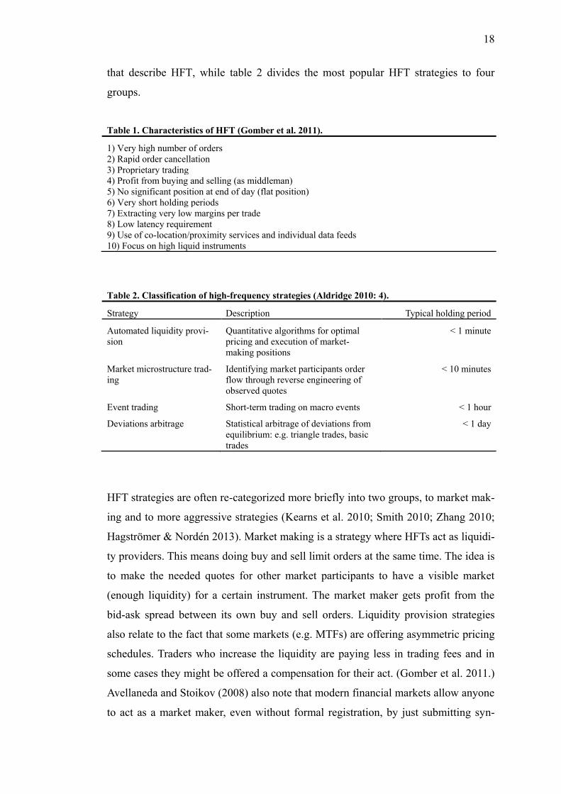
number of orders (Zhang 2010; Gomber et al. 2011). Table 1 lists common features
8For stylized facts about HFT profitability, the reader is pointed to Baron et al. (2012).
18
that describe HFT, while table 2 divides the most popular HFT strategies to four
groups.
Table 1. Characteristics of HFT (Gomber et al. 2011).
1) Very high number of orders
2) Rapid order cancellation
3) Proprietary trading
4) Profit from buying and selling (as middleman)
5) No significant position at end of day (flat position)
6) Very short holding periods
7) Extracting very low margins per trade
8) Low latency requirement
9) Use of co-location/proximity services and individual data feeds
10) Focus on high liquid instruments
Table 2. Classification of high-frequency strategies (Aldridge 2010: 4).
Strategy Description Typical holding period
Automated liquidity provi-
sion
Quantitative algorithms for optimal
pricing and execution of market-
making positions
< 1 minute
Market microstructure trad-
ing
Identifying market participants order
flow through reverse engineering of
observed quotes
< 10 minutes
Event trading Short-term trading on macro events < 1 hour
Deviations arbitrage Statistical arbitrage of deviations from
equilibrium: e.g. triangle trades, basic
trades
< 1 day
HFT strategies are often re-categorized more briefly into two groups, to market mak-
ing and to more aggressive strategies (Kearns et al. 2010; Smith 2010; Zhang 2010;
Hagströmer & Nordén 2013). Market making is a strategy where HFTs act as liquidi-
ty providers. This means doing buy and sell limit orders at the same time. The idea is
to make the needed quotes for other market participants to have a visible market
(enough liquidity) for a certain instrument. The market maker gets profit from the
bid-ask spread between its own buy and sell orders. Liquidity provision strategies
also relate to the fact that some markets (e.g. MTFs) are offering asymmetric pricing
schedules. Traders who increase the liquidity are paying less in trading fees and in
some cases they might be offered a compensation for their act. (Gomber et al. 2011.)
Avellaneda and Stoikov (2008) also note that modern financial markets allow anyone
to act as a market maker, even without formal registration, by just submitting syn-
19
chronized limit orders. Usually these HFT market making strategies are not seen as
the source of controversy because market making is not directional trading and its
profits are not related to price trends (see Guilbaud & Pham 2013). In comparison,
aggressive strategies include for example directional trading activities and arbitrage
strategies such as the ETF arbitrage (Hagströmer & Nordén 2013).
4.3 How to spot a player?
There are still many unanswered questions and problematic issues related to HFT
data gathering and reliability for research purposes. We clearly need a broader data
and longer time periods as most of the critic given to existing literature relates to
these two issues. HFT research has so far been over-representing the short-term ef-
fects while the long-term effects might be more economically meaningful. One prob-
lem in academic research is the difficulty to determine the unobservable HFT activi-
ty. As noted by Cartea and Penalva (2012), the huge task of empirical HFT research
is to find a way to study HFT indirectly, using proxies of different trading behavior.
Publicly available information about trading does not include identifiers for different
traders, which makes it hard to dissolve the high-frequency strategies for research
(Cartea & Jaimungal 2013).
One major difficulty is to identify order-by-order from the data which trade has been
HFT activity. So far there has been different measures to categorize traders (e.g. Al-
dridge 2010; Zhang 2010; Kirilenko et al. 2011; Hasbrouck & Saar 2013), but clearly
there should be better and more specific ways. Gomber et al. (2011) suggest that in
order to find the best method, researchers should do more co-operation with the mar-
ket participants using HFT strategies. This could be a way to have more reliability as
HFT activity is often related to trades in dark pools. These have very limited amount
of data available for research purposes.
Hagströmer and Nordén (2013) point out that one caveat in academic research is the
difficulty to address different HFT and AT strategies individually. The division is
important in order to objectively investigate the real impacts of such activities as it is
not reasonable to consider them as a whole. This categorization of traders and strate-
gies is, however, problematical as traders usually do not use only one strategy. They
20
can change their strategies and methods in relation to market situations. This leads to
difficulties if the research is done by dividing HFT activity using trader identifiers.
Hasbrouck and Saar (2013) introduce a framework to study HF activity from ex-
change message data which has the advantage that it can be constructed from public-
ly-available data. Like other measures, this is a proxy of HFT activity which causes
some drawbacks being just a directional estimate. Other researchers have acquired
unique data sets in co-operation with exchanges, for example Brogaard (2010) and
Brogaard et al. (2013a) used a data set provided by NASDAQ which identified HFT
as a specialized proprietary traders leaving out the HFT activity stemming from larg-
er traders like investment banks. Problems with unique data sets are also related to
issues in robustness as replicating and verifying the results may be difficult or even
impossible.
Researchers have also been using exogenous technology shocks on market infra-
structure as a circumstance which assumedly amplifies HFT activity (see Zhang
2010; Hendershott & Moulton 2011; Riordan & Storkenmaier 2012; Brogaard et al.
2013b). Because these technological advantages allow lower latency they are seen as
a turning point in high speed trading. By comparing the time period before and after
such an improvement we should be able to see some of the HFT effects. Hendershott
and Moulton (2011) examine the introduction of NYSE’s Hybrid Market in 2006 and
find that the following time period was characterized by increased spreads and im-
proved price discovery processes. Similar study conducted by Riordan and
Storkenmaier (2012) finds that the improvements in Deutsche Boerse Xetra system
also enhanced liquidity measures in the post-shock period.
Smith (2010) gives useful details about the two remarkable market infrastructure
changes that occurred in the last decade. First was the decimalization of U.S. price
quotes, followed by SEC’s revision of Regulation National Market System (Reg.
NMS) which started in August 2005. This automated trading system allowed more
high speed transactions, and it is generally thought to be the excuse for mushrooming
HFT activity. Usually the effects of Reg. NMS are measured from 2005 and after
(e.g. Smith 2010), but a closer look to SEC’s (2007) report on the implementation of
21
Reg. NMS reveals that the final phase of renovations started as late as July 9th 2007
and reaching its full completion at October 8th 20079.
4.4 A new normal in risk management
A possibility for a rogue algorithm raises discussion about extreme events which
could be caused by sudden liquidity removal by HFTs. Liquidity withdrawal has
been proved to increase in extreme market movements. In the case of HFT this
would happen by suddenly removing the market makers buy and sell orders from the
order book. (CFTC-SEC 2010; Easley et al. 2011; Gomber et al. 2011.)
For example in the Flash Crash, HFTs applying market making strategies suddenly
stopped providing liquidity as they pulled off their orders. They were not the first
cause of the problems but they reacted as the markets were showing unusual move-
ments and high volatility. This reaction caused exacerbating volatility and price
movements. As this incident shows, HFT can work in both ways as it can provide
liquidity and in extreme cases take liquidity from the markets. More information
about HFT activity and its appearance during the Flash Crash can be found from
CFTC-SEC (2010), Kirilenko et al. (2011) and Ben-David et al. (2012).
Zhang (2010) notes that HFTs can stop their market making and other trading activi-
ties if they spot market conditions that are making it difficult to gain profits or ex-
pose them to inventory risks. Bearing inventory that they do not want to hold would
lead to abnormal levels of sell orders. When everyone lines up on the same side of a
trade, the liquidity shows up as an illusion. This kind of position could appear during
high market uncertainty, in a situation where some external cause is amplifying vola-
tility.
Madhavan (2012) notes that employing circuit breakers at a stock specific level can
be helpful in times of market stress like in the Flash Crash, but they also can cause
some problematic issues. When price movements are stopped at an individual stock
9This final phase of Reg NMS is related to Rule 610 and Rule 611, which are the most notable rules
related to market system automation, market access, and to quote priorities.
22
level, these restrictions can complicate the pricing process of ETFs, whose prices are
determined by the underlying securities basket. Such a situation can cause unex-
pected ETF mispricing in times of high volatility. In relation to these ideas, Gomber
et al. (2011) note that a significant amount of the problems related to HFT might be
caused by U.S. market structures. They compare the situation in U.S. to European
markets which have for long used a volatility safeguard regime. So far no market
quality related issues with HFT have been noticed in European markets.
HFT activity faces different risks than normal, not latency dependent, trading. Cartea
and Jaimungal (2013) argue that commonly used risk metrics (e.g. VaR, ES) are es-
pecially invented for trading strategies that are not dependent on trading speed, and
therefore these metrics cannot serve for HFT as their risk controls. Of course it is not
assumed that HFTs would rely on such measures in their trading, but it clearly shows
the need for developing some risk metrics especially for HFT10
.
Various sources consider the introduction of financial transaction tax with the aim to
reduce the possible harmful side of high-frequency trading (e.g. Biais & Woolley
2012; Cohen & Szpruch 2012). It is worth noting that the aim of such tax would only
be to prevent predatory trading, not the whole range of different HFT strategies. Jar-
row and Protter (2012) argue in line that regulators should adjust the policies to ex-
clude the predatory aspect of HFT. Cohen and Szpruch (2012) state that, the transac-
tion tax might even improve the overall market efficiency by making the market
more attractive to slower traders.
10For comprehensive qualitative discussion on HFT related risks see GOS (2012).

23
5 THEORETICAL FRAMEWORK
5.1 Arbitrage in financial markets
A typical text book arbitrage is defined as an opportunity to gain profits without nei-
ther capital nor risk. The theoretical concept of arbitrage is explained by Sharpe and
Alexander (1990) with the definition of: “…the simultaneous purchase and sale of
the same, or essentially similar, security in two different markets for advantageously
different prices“. These arbitrage opportunities appear to be in some extent different
in reality. Shleifer and Vishny (1997) argue that in real financial markets specialized
investors take part in arbitrage activity even if it needs capital and exposes them to
various risks. In modern markets these specialized investors include hedge funds,
proprietary trading desk in big banks, and HFTs11
.
Availability of low risk capital is necessary to take advantage of thin arbitrage oppor-
tunities. As the cost of financing rise, say with market stress, arbitrage activities
might have to be scaled back. This is due to the fact that market mispricing, like ETF
premiums, might stay longer than expected in volatile markets. In some cases the
observed mispricing might grow bigger due to similar reasons. A rational arbitrageur
has to consider the cost of financing, which also rises in relation to market stress,
before partaking into the arbitrage. Davidson (2013) argues that the ability to do arbi-
trage trading is a function of available financing and of the risks related to the arbi-
trage. According to Brunnermeir et al. (2009) VIX index can serve as a simplified
measure for available arbitrageurs’ capital. As volatility begets volatility the capital
needs and arbitrage risks can be qualitatively and reasonably related to the VIX in-
dex, other proxies for high volatility, and measures of financing costs of short-term
trading activities.
11It is important to note that HFT is often done by hedge funds, and not solely by proprietary trading
firms. The difference between these two definitions is the source of trading capital: Hedge Funds
usually use money from their investors while proprietary traders use their own money (or loans). Nev-
ertheless, the effects of these two HFTs are the same and during this study hedge fund based HFT
activity is considered in line with other possible sources of HFT.
24
The unique arbitrage mechanism behind ETF pricing process differs in some manner
from the traditional concept of arbitrage. As explained in the terminology, this mech-
anism is a contract based relationship between the authorized participant and the is-
suer of the ETF. The creation/redemption process is unlike from other arbitrage sit-
uations as in consequence an amount of ETF shares actually is made or redeemed
from the markets. This mechanism allows a pure risk-free profit for the AP as long as
the prevailing price gap between ETF and NAV is wide enough. It is worth noting
that limits of arbitrage are mitigated as the ETF share creation/redemption takes
place in primary markets, not in the actual secondary marketplace. More importantly,
this exchange takes place on a fair value basis, not with the price the ETF is trading
at the secondary markets. What makes the overall concept of ETF arbitrage more
complicated is that any other trader is free to arbitrage with ETFs in the secondary
market. Therefore, the ETF creation and redemption process is not the only arbitrage
force behind ETF pricing process.
5.2 Understanding ETF arbitrage at high-frequency
Simple mean-reverting (pairs trading) strategies work better for ETF pairs and tri-
plets than for stocks. This is due to the fact that ETFs are often highly diversified and
hence their fundamental economics do not change as quickly as corporate stocks’
(Marshall et al. 2010; Chan 2013). This indicates that ETFs form an attractive range
for the algorithmic mean-reverting strategies. ETFs can also be used as a second in-
strument in a classical index arbitrage where trades are based on the differences in
values of a portfolio of stocks (such that form an index, say S&P 500) and their cor-
responding ETF (in this case SPY). Classical as it is, such a common strategy has
been noted and the profits grown thinner since (Reverre 2001). Chan (2013) argues
that these thin profits can still be highly attractive, especially if traded intraday at
high-frequency. Due to their relative speed advantage high-frequency traders can
exploit the intraday index arbitrage by using ETFs and their underlying assets.
Ben-David et al. (2012) argue that ETF arbitrage is mainly done by HFTs. This is
also seen as a reason why HFT activity can have impacts on market quality measures
as volatility, and in time of market stress HFT activity may cause serious market dis-
ruptions. ETF arbitrage can be harder due to the limits of arbitrage which are more

25
relevant when the underlying asset basket is difficult to trade. This might be because
of issues related to its liquidity or other complex characteristics. Mainly this is con-
nected to small illiquid funds and to non U.S. based funds whose assets baskets trade
at non-synchronized times with the fund itself (Engle & Sarkar 2006). Although larg-
er ETFs face more often creation/redemption processes than smaller and less traded
funds, the creation units account only a fraction of the total daily volume because of
remarkable higher trading volume (Petäjistö 2011). Therefore, secondary market ar-
bitraging between ETFs and their asset baskets is more suitable in large U.S. based
funds as the arbitrageurs’ trading cannot be offset by a single creation unit. The at-
tractiveness of these funds for arbitraging is also affected by the fact that their under-
lying securities are traded simultaneously, making limits of arbitrage less significant.
Remarkably, U.S. market traded ETFs have also been found to trade with different
prices than their net asset value would suggest. Even though this difference is partly
supposed to be mitigated by authorized participants in ETF creation and redemption
process (Petäjistö 2011; Ben-David et al. 2012), it still seems that this activity is in-
adequate to push the premiums to zero. Still prevailing thin profits might be enough
to attract other arbitrageurs to arbitrage between the ETFs and their underlying as-
sets12
. As noted by Chan (2013), thinner profits require higher trading frequency
which makes this arbitrage solely tempting to HFTs.
Petäjistö (2011) finds that the average volatility of the closing price premium in all
ETFs is 53 basis points. He also shows that, although, these premiums are more vola-
tile for smaller and illiquid funds, the premium is still significant for the biggest and
most liquid funds. Petäjistö (2013) continues with these findings in a detailed man-
ner, showing that in early 2007 the cross-sectional premium volatility was 25 bp, but
it increased significantly for the whole 2008, peaking in September 2008. Other
times of high premium volatility are noted around the Flash Crash in May 2010, and
during November 2010 muni-bond crash.
12It is worth noting that ETF arbitrage can also take place between the ETFs and their relevant futures.
See Richie et al (2008) and Ben-David et al. (2012) for more information on the usage of futures in
these trading activities.
26
This premium volatility serves as an interesting measure to address the arbitrage ac-
tivity between ETFs and their underlying assets. The premium volatility can be am-
plified in times of market stress which motivates us to investigate the matter in more
detail. For example, having limit orders in the ETF at the moment of abnormally
high premium volatility can lead to unwanted trades as the trade can be executed
even though the NAV has not triggered this threshold. This is clearly an important
issue for ETF investors as it might reduce the attractiveness to invest in ETFs by hav-
ing severe economic influences.
27
6 RESEARCH DESIGN AND RESEARCH QUESTIONS
6.1 Research problems and methodology
This paper aims to contribute in connecting the HFT activity to ETF pricing process
by demonstrating HFTs’ role in ETF arbitrage activity. This is done by constructing
simple factor models to explain the level of ETF mispricing and its volatility. OLS
regression analysis is then used to estimate the relationship between ETF mispricing
and the chosen features. These multivariate linear regressions take the following lin-
ear equation form:
, (1)
where is the observed ETF mispricing at time t (when ),
is the vector of regression coefficients including constant, contains a dummy for
constant term and each relevant predictor variable, including also the lagged varia-
bles, and is the error term. After considering possible multicollinearity issues, the
linear regression analysis is performed to all predictor variables, and then dropping
out one by one the non-significant variables13
and the independent variables with the
smallest absolute t-statistics. Appendix I, shows the full list of independent variables
the analysis was started with, while empirical results document only the most statisti-
cally, economically, and qualitatively meaningful variables.
Another purpose of this paper is to address HFTs’ role in ETF mispricing in a de-
tailed manner and formally test if the noted change in ETF mispricing trend is con-
nected to the rise of HFT. This is conducted by utilizing an exogenous technology
shock which improved market infrastructure to make it more suitable for HFT activi-
ties. By addressing the time periods before and after such a shock we should see
strengthened HFT activity and its effects in a distinguishable manner. Similar meth-
odology is used in Hendershott and Moulton (2011) and Riordan and Storkenmaier
(2012) to study HFT effects on stock markets.
13Non-significance is measured as - .
28
The technology shock, Reg. NMS, which reduced trading latency, was proposed to
have started at 2005, but due to extensions required by market operators it reached its
full capacity at the 8th of October 2007 (see SEC 2007; Smith 2010; Madhavan
2012; Pagnotta & Philippon 2012). This renovation of market routing infrastructure
also affected NYSE Arca which is the main exchange for ETFs. The methodology
for testing the significance of this technology shock is done by applying the Chow
test (see Chow 1960). This is used to test if the coefficients in the multivariate and
univariate linear regressions have changed prior and after the technology shock,
which serves as a structural break in the data set. We divide the original multivariate
linear regression into two set of equations. The mathematical expression of this com-
bined model with breaks is as follows:
, (2)
where is a dummy variable getting values 0 and 1 in relation for a given break point
such that if and zero otherwise, is a vector indicating the change in
intercept and is a vector containing the changes in slope parameters, while is the
design matrix containing every relevant predictor variable, is the vector of regres-
sion coefficients, and is a vector for the external expression for the intercept term.
This model has constant parameters only if = = 0. Thus the hypotheses for testing
are: against . This is tested by calculat-
ing the Chow test statistic:
–
, (3)
where RRSi stands for the sum of squared residuals for the combined data and the
two groups with split data when . The number of observations in each
group is given by and while is the total number of parameters. The Chow test
statistics then follows the F-distribution with and degrees of free-
dom.
As has been proposed by Davidson (2013) and Petäjistö (2013), ETF pricing struc-
tures have changed remarkably after 2007 and the relationship between ETF mispric-
29
ing and various exogenous factors have twisted. Prior to that time only a limited
amount of ETFs were traded and their assets under management have faced similar
developments. This arguably affects the cross-section of ETFs but should not con-
cern in such a magnitude the largest ETFs with distant inception dates. Both authors
emphasize that the transition in ETF mispricing trend might be due to maturation of
ETF markets. One can argue that these explanations are without exhaustive qualita-
tive background. Accordingly, Davidson (2013) notes that the turning point in Janu-
ary 2007 is arbitrary, to result in satisfying connection with the maturation of ETF
markets and developments in arbitrage behavior. Appearance of sophisticated arbi-
trageurs who could be able to engage in arbitrage trading even with thin profits and
high-frequency might serve as an explanation for the changes in ETF mispricing
trends. This is also in part missed by Davidson (2013) and Petäjistö (2013) as the
main renovations to market infrastructure which allowed more HFT activity occurred
actually in 2007 (see SEC 2007). Therefore, it is logical to set the structural break
point at this Reg. NMS implementation point in order to relate the effects to height-
ened HFT activity.
In addition to considering the regression results separately for time periods prior and
after the Reg. NMS, different statistical tools are employed to analyze the relation-
ships with independent factors and ETF premiums and the possible structural breaks
in these time-series in a more detailed manner. Namely these tools include rolling
regression analysis, estimating time-varying betas with Kalman filter method, and a
test based on the cumulative sum of recursive residuals (Rec-CUSUM).
Finally, we aim to contribute to existing literature by updating ETF premium volatili-
ty modeling to incorporate the possible changes in ETF mispricing trend in post-
2007 era. The ETF premium volatility process is modeled by employing Generalized
AutoRegressive Conditional Heteroskedastic (GARCH) volatility model using HFT
related exogenous regressors. Being able to model the premium volatility can be use-
ful for example in risk-management as limit orders in ETFs might be executed unfa-
vorably in times of high premium volatility. Such a situation might occur when ETF
return differs from the underlying index triggering the limit order even when the un-
derlying index return does not exceed such a threshold.

30
Using a GARCH model, we can model the conditional variance of the time-series
(see Engle 1982; Bollerslev et al. 1994; Tsay 2005). GARCH models have the bene-
fit of modeling more accurately the volatility clustering phenomena which means
that the time-series includes recognizable periods of high and low volatility. The em-
ployed volatility model is expressed as follows: For the log ETF mispricing series ,
let be the innovation at time t. Then follows a GARCH(p,q) model if
, -
- , (4)
where , , , and , is a sequence of iid
random variables with mean 0 and variance of 1. With the entertained model to
match the best the characteristics of log SPY premium time-series we use
GARCH(1,1) including exogenous regressors for forecasting purposes. The model
selection process is explained in a detailed manner in empirical results, while the
equation for the final chosen model is presented here:
, - - - , (5)
where is the vector for exogenous variables and follows Student’s t-
distribution.
6.2 Research questions and objective
Summarized research questions:
Can ETF premium and its volatility (end-of-day) be partly explained by fac-
tors related to HFT activity?
Are ETF premium time-series evolution affected by heightened HFT activity
as measured by the implementation of Reg. NMS?
Research objective:
GARCH modeling ETF premium volatility using exogenous regressors relat-
ed to HFT activity.

31
7 RESEARCH DATA
7.1 Data description and sources
The empirical part mainly focuses on the SDPR trust (SPY) during a time period
from 2nd of January 2002 to 15th of January 2013. The time period relies on several
explanations: As SEC ordered all U.S exchanges to convert their quotes to decimals
instead of eights of a dollar on April 9th 2001, it is reasonable to consider only the
time period after this time point. It is logical to assume that a significant amount of
ETF premiums have been due to quotation standards prior the decimalization (see
Chen et al. 2008). HFT activity is also assumed to have benefited from this change.
Another turning point for HFT is the renovation of U.S. exchanges by implementa-
tion of Reg. NMS (July 9th 2007). The examined time period is chosen to reflect
equal lengths prior and after this technology shock.
This research concentrates solely on the SPY as it is the largest U.S based ETF. It is
worth emphasizing that the aim is not to explain cross-sectional ETF premium dif-
ferences. We are merely looking for an introductory framework to relate HFT and
their effects on exchange-traded products. Another relevant issue in research on ETF
premiums is the stale pricing of certain bond funds and non-U.S. based funds. As has
been noted in Petäjistö (2011) and Davidson (2013), stale pricing and non-
synchronous trading are significant factors behind ETF premiums. These findings
serve as a motive to ignore non-U.S based ETFs in this study. Although, different
methods has been introduced to address the stale pricing issue (see Engle & Sarkar
2006; Petäjistö 2013), doing so is out of the scope of a Master’s Thesis. An addition-
al matter in non-synchronous trading is the fact that many ETFs (including SPY)
traded on AMEX, until November 2008, 15 minutes longer than the underlying U.S.
equities (Petäjistö 2013). This also concerns the results in this study, but from the
accessible data sources it is impossible to correct.
Focusing the research only on SPY serves one more topic: It is reasonable to assume
that the cross-sectional ETF market dynamics have evolved around 2007 for the rea-
son stated by Davidson (2013) and Petäjistö (2013), where they namely mean the
maturation of ETF markets. As SPY has been around since 1993, and being the big-
32
gest, most liquid, and most traded ETF, its micro-market structures must have been
developed far earlier. The characteristics of prior-2007 ETF marketplace are mainly
due to limited amount of funds in the ETF universe. Thus, addressing the pricing
dynamics of only SPY can serve as a reasonable way to dissect the effects of ETF
market maturation from the assumed effects caused by heightened HFT activity,
which both occurred in a fairly overlapping time point. The change in cross-sectional
ETF pricing dynamics is far more difficult to explain following the methodology
used in this study as the effects of these two phenomena might merge.
ETF daily price, trading volume, NAV data, number of outstanding shares, and daily
high and low prices are obtained from Bloomberg. Thomson Reuters Datastream is
used to construct the relevant Fung-Hsieh Mutual Fund factors while multiple other
sources are used to construct the other explanatory variables (See Appendix I for
complete data sources).
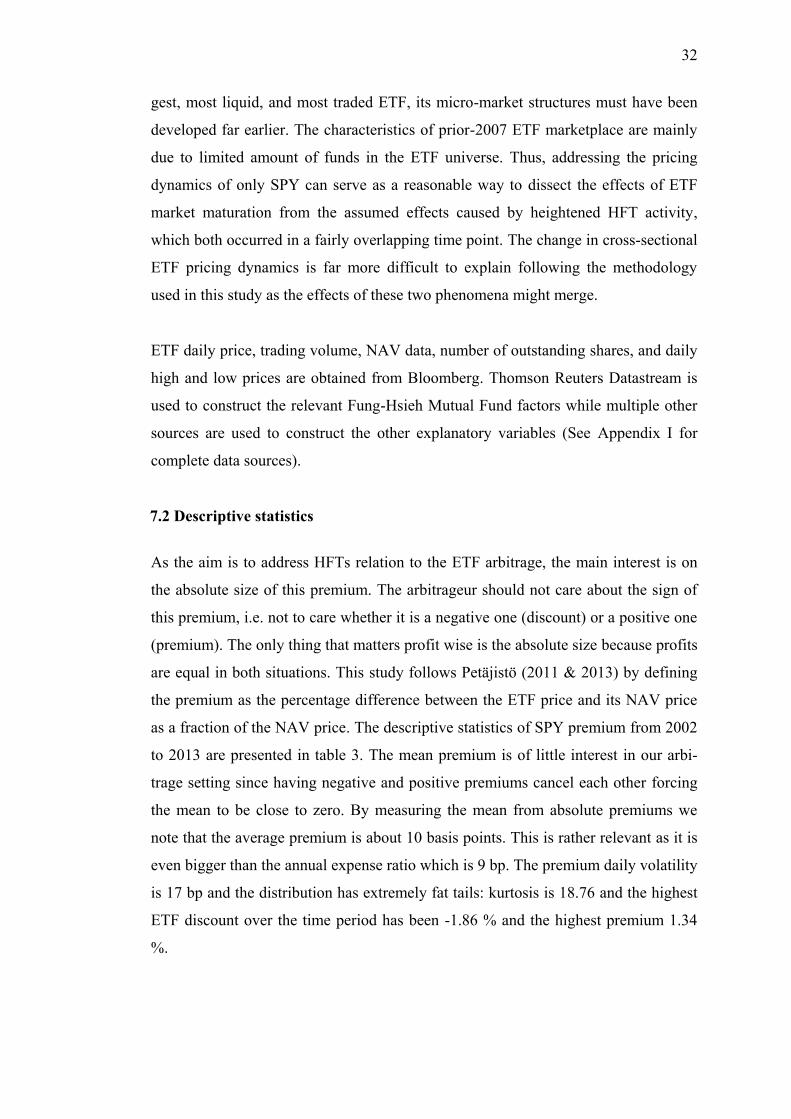
7.2 Descriptive statistics
As the aim is to address HFTs relation to the ETF arbitrage, the main interest is on
the absolute size of this premium. The arbitrageur should not care about the sign of
this premium, i.e. not to care whether it is a negative one (discount) or a positive one
(premium). The only thing that matters profit wise is the absolute size because profits
are equal in both situations. This study follows Petäjistö (2011 & 2013) by defining
the premium as the percentage difference between the ETF price and its NAV price
as a fraction of the NAV price. The descriptive statistics of SPY premium from 2002
to 2013 are presented in table 3. The mean premium is of little interest in our arbi-
trage setting since having negative and positive premiums cancel each other forcing
the mean to be close to zero. By measuring the mean from absolute premiums we
note that the average premium is about 10 basis points. This is rather relevant as it is
even bigger than the annual expense ratio which is 9 bp. The premium daily volatility
is 17 bp and the distribution has extremely fat tails: kurtosis is 18.76 and the highest
ETF discount over the time period has been -1.86 % and the highest premium 1.34
%.
33
Table 3. Descriptive statistics of daily ETF mispricing, mean of the absolute size of ETF mispric-
ing, and annualized premium volatility.
SPY Premium
Mean -0.01 %
abs(Mean) 0.10 %
SD (daily) 0.17 %
SD (annual) 2.64 %
Skewness -1.25
Kurtosis 18.76
Min -1.86 %
Max 1.34 %
N 2751
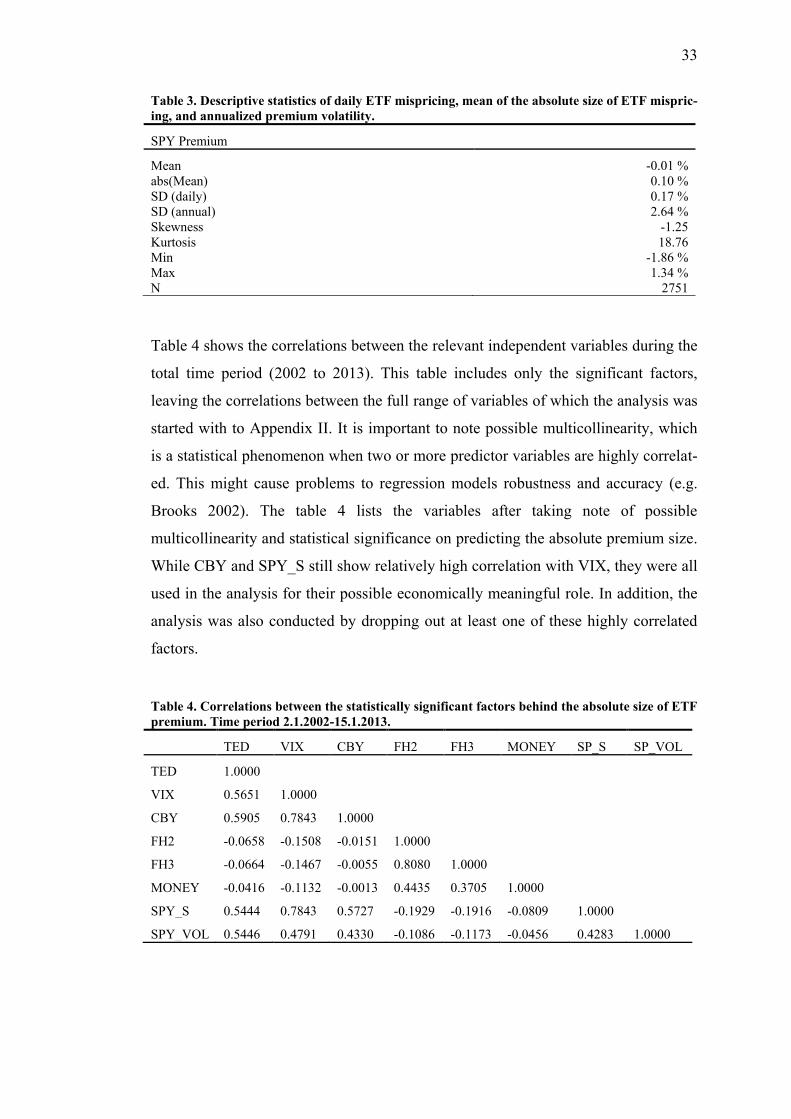
Table 4 shows the correlations between the relevant independent variables during the
total time period (2002 to 2013). This table includes only the significant factors,
leaving the correlations between the full range of variables of which the analysis was
started with to Appendix II. It is important to note possible multicollinearity, which
is a statistical phenomenon when two or more predictor variables are highly correlat-
ed. This might cause problems to regression models robustness and accuracy (e.g.
Brooks 2002). The table 4 lists the variables after taking note of possible
multicollinearity and statistical significance on predicting the absolute premium size.
While CBY and SPY_S still show relatively high correlation with VIX, they were all
used in the analysis for their possible economically meaningful role. In addition, the
analysis was also conducted by dropping out at least one of these highly correlated
factors.
Table 4. Correlations between the statistically significant factors behind the absolute size of ETF
premium. Time period 2.1.2002-15.1.2013.
TED VIX CBY FH2 FH3 MONEY SP_S SP_VOL
TED 1.0000
VIX 0.5651 1.0000
CBY 0.5905 0.7843 1.0000
FH2 -0.0658 -0.1508 -0.0151 1.0000
FH3 -0.0664 -0.1467 -0.0055 0.8080 1.0000
MONEY -0.0416 -0.1132 -0.0013 0.4435 0.3705 1.0000
SPY_S 0.5444 0.7843 0.5727 -0.1929 -0.1916 -0.0809 1.0000
SPY_VOL 0.5446 0.4791 0.4330 -0.1086 -0.1173 -0.0456 0.4283 1.0000

34
TED spread and VIX index are serving as proxies for available arbitrageurs’ capital
while CBY (Corporate Bond Yield) is a bond oriented risk factor. FH2 and FH3 are
the only relevant factors from the Fung-Hsieh Mutual Fund risk factor list14
, which
was used to serve as a naive proxy for different funds’ behavior. The main idea was
to estimate hedge fund activity but as Fung-Hsieh Hedge Fund factors15
are not ap-
plicable at a daily level, the mutual fund factors were used instead with relevant bond
oriented risk factors. MONEY is Kenneth French’s Financial Industry portfolio
which is used to serve as a proxy for financial industry’s state of nature. While it also
correlates highly with wide equity indexes like S&P 500 it also captures U.S. market
returns and their effects. SPY_S is a simple estimate of realized daily ETF volatility
and SPY_VOL is a feature scaled measure of SPY daily volume. SPY_S and
SPY_VOL serve as ETF endogenous factors related to HFT activity on the ETF on a
specific day: high daily volatility might cause lower HFT activity as it introduces
risks to arbitrage while higher than usual trading volume can indicate high HFT ac-
tivity as they generate a lion’s share of market volumes.
These two endogenous ETF factors are naive measures for HFT activity and its con-
straints. We recognize that these measures may not be the most relevant proxies for
HFT activity and a lot of simplified assumptions had to be done in order to be con-
tent in their usage. We also searched for ETF quotation data for a better HFT proxy.
By constructing a quote-to-trade ratio we could have build a more satisfactory HFT
measure as their behavior has been noted to be highly related to the amount of non-
executed trades, i.e. quotes, while using only trading volumes can capture only a
messy estimate of HFT activity. The accessible data sources did not provide quota-
tion information, leaving our HFT activity estimation to a fairly unsatisfactory level.
The relationship between the chosen factors and the absolute size of observed ETF
premiums is assumed to be linear to justify the use of mostly linear approach for re-
search purposes. Theoretically this assumption is based on the idea of vanishing arbi-
trage profits: if at some point ETF premiums show arbitrage opportunities (i.e. high
14See https://faculty.fuqua.duke.edu/~dah7/8FAC.htm for the full 8-factor list of these factors. Not all
are applicable at daily level. 15See https://faculty.fuqua.duke.edu/~dah7/HFRFData.htm for the Hedge Fund 7-factor list.

35
premiums), the arbitrageurs’ are assumed to trade on these opportunities forcing the
ETF premiums to shrink (i.e. no observable premiums). Therefore, the factors which
are related to constrained arbitrage activity should have positive linear relationship
between absolute premiums while the factors related to higher arbitrage activity
should have negative linear relationship with absolute ETF premiums.

36
8 EMPIRICAL RESULTS
8.1 The factors behind ETF premiums
Appendix III shows the time-series evolution of SPY premium over the time period.
The premium shows some amount of time persistence as high premium volatility
occurred in the early part of the time period and during the years of the financial cri-
sis. After the crisis the premiums have shrank and their volatility reduced significant-
ly. SPY realized daily volatility also shows turbulence during 2002 to 2003, in finan-
cial crisis, and again during the Flash Crash.
Regression analysis run on ETF premium tries to capture how the actual level and
sign of ETF premiums could be predicted similarly to stock returns. Table 5 presents
regression results using ETF premium as the dependent variable. The only statistical-
ly significant 1-day lagged factors are SPY_S, VIX, and MONEY. R2 is rather low (3
%) showing that the actual level of ETF premiums is not predicted with accuracy at
least on short-term. When considering the arbitrageurs’ role in ETF mispricing the
exact level of ETF premium is less interesting than the absolute size of the premium.
This is because the aim is to explain the factors which are connected to widening or
shrinking premiums ignoring whether the premium is negative or positive.
Table 5. Regression results using daily data and actual level of ETF premium as the dependent
variable. This is defined as (ETF-NAV)/NAV. Independent variables are lagged one day. Time
period is from 02.01.2002–15.01.2013.
(1) (2) (3)
Intercept 0.0247 ***
(4.80)
0.0034
(0.43)
0.0005
(0.07)
SPY_St-1 -2.1363 ***
(-7.84)
-3.3508 ***
(-7.65)
-3.3698 ***
(-7.71)
VIXt-1 0.0018 ***
(3.53)
0.0020 ***
(3.80)
MONEYt-1 0.0055 ***
(3.40)
N 2750 2750 2750
Adj. R2 0.02 0.03 0.03
N = number of observations, t-values in parentheses,
* = 0.05 level of significance, ** = 0.01 level of significance, and *** = 0.001 level of significance.

37
Table 6 presents the regression results using absolute size of the ETF premium as a
dependent variable. The time period covered is from start of 2002 to January 2013.
In the result interpretation we should note that in a perfect world where no arbitrage
opportunities would exist, we would see absolute premium of zero. Therefore, the
factors behind constrained arbitrage activity should show have positive coefficients
while the factors behind higher HFT activity related to ETF arbitrage should show
negative coefficients.
The analysis shows that ETF endogenous factors (SPY_S and SPY_VOL) are major
contributors to SPY premiums. The R2 is 21 % using lagged 1-day values of these
two factors. SPY_S, which measures the realized daily SPY volatility, is highly sta-
tistically significant and is also qualitatively reasonable as high volatility may lead
HFTs and other arbitrageurs to scale back their activities. High value of SPY_VOL is
understood to proxy higher than usual trading volume, and as a result also higher
HFT activity. Higher arbitrage activity leads to lower premiums as ETF prices revert
towards the NAV value. TED spread and VIX also have the expected coefficient sign
as constrained arbitrage activity should cause the premiums to grow even wider as
arbitrageurs may not be able to participate into trading activities.
Table 7 shows the regression results using 5-day SPY premium volatility as the de-
pendent variable. This tries to reveal if the factors behind the time persistence of
premium volatility are the same as the factors explaining the absolute daily premium
size. The daily realized SPY premium volatility is calculated by taking the average of
daily squared returns over each five day period and taking a square root of this value.
This partly follows the methodology recommended by Hasbrouck (2007) where we
set the in variance calculations equal to zero. For the regression analysis we will
use 5-day averages of the independent variables. The results are presented using
overlapping and non-overlapping 5-day periods where the non-overlapping lagged
( values represent the last week averages of these factors.
The analysis tells similar story as the regressions run on daily variables. The results
are also qualitatively the same using non-overlapping and overlapping observations:
SPY_S, SPY_VOL, and TED remain the most powerful explanatory variables with
the expected coefficient signs.
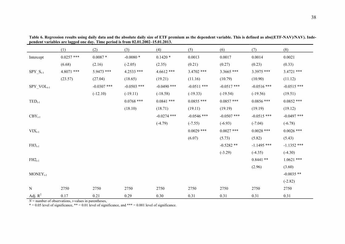
38
Table 6. Regression results using daily data and the absolute daily size of ETF premium as the dependent variable. This is defined as abs((ETF-NAV)/NAV). Inde-
pendent variables are lagged one day. Time period is from 02.01.2002–15.01.2013.
(1) (2) (3) (4) (5) (6) (7) (8)
Intercept 0.0257 ***
(6.68)
0.0087 *
(2.16)
-0.0080 *
(-2.05)
0.1420 *
(2.35)
0.0013
(0.21)
0.0017
(0.27)
0.0014
(0.23)
0.0021
(0.33)
SPY_St-1 4.8071 ***
(23.57)
5.9473 ***
(27.04)
4.2533 ***
(18.65)
4.6612 ***
(19.21)
3.4702 ***
(11.16)
3.3665 ***
(10.79)
3.3975 ***
(10.90)
3.4721 ***
(11.12)
SPY_VOLt-1 -0.0307 ***
(-12.10)
-0.0503 ***
(-19.11)
-0.0490 ***
(-18.58)
-0.0511 ***
(-19.33)
-0.0517 ***
(-19.54)
-0.0516 ***
(-19.56)
-0.0515 ***
(19.51)
TEDt-1 0.0768 ***
(18.10)
0.0841 ***
(18.71)
0.0855 ***
(19.11)
0.0857 ***
(19.19)
0.0856 ***
(19.19)
0.0852 ***
(19.12)
CBYt-1 -0.0274 ***
(-4.79)
-0.0546 ***
(-7.55)
-0.0507 ***
(-6.93)
-0.0515 ***
(-7.04)
-0.0497 ***
(-6.78)
VIXt-1 0.0029 ***
(6.07)
0.0027 ***
(5.73)
0.0028 ***
(5.82)
0.0026 ***
(5.43)
FH3t-1
-0.5282 **
(-3.29)
-1.1495 ***
(-4.35)
-1.1352 ***
(-4.30)
FH2t-1 0.8441 **
(2.96)
1.0621 ***
(3.60)
MONEYt-1 -0.0035 **
(-2.82)
N 2750 2750 2750 2750 2750 2750 2750 2750
Adj. R2 0.17 0.21 0.29 0.30 0.31 0.31 0.31 0.31
N = number of observations, t-values in parentheses,
* = 0.05 level of significance, ** = 0.01 level of significance, and *** = 0.001 level of significance.
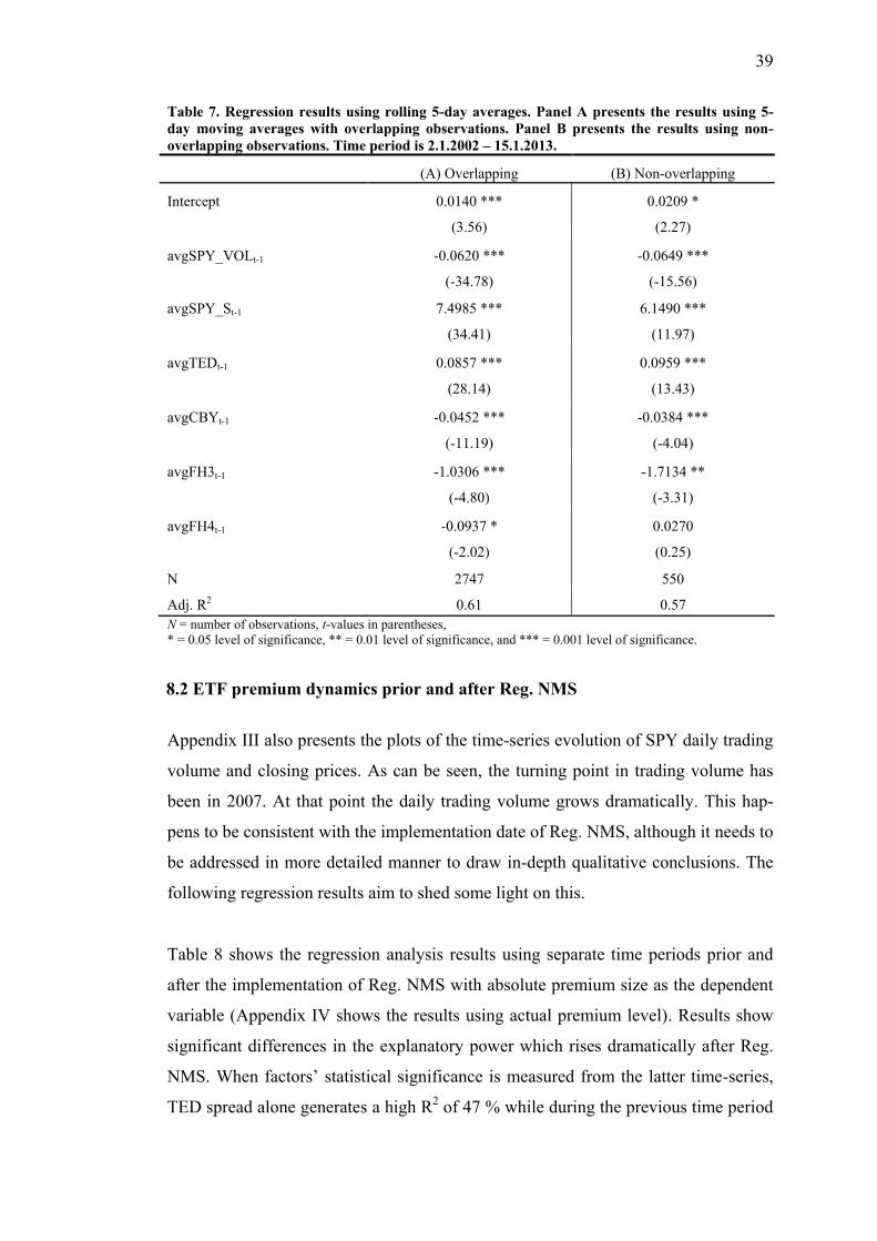
39
Table 7. Regression results using rolling 5-day averages. Panel A presents the results using 5-
day moving averages with overlapping observations. Panel B presents the results using non-
overlapping observations. Time period is 2.1.2002 – 15.1.2013.
(A) Overlapping (B) Non-overlapping
Intercept 0.0140 ***
(3.56)
0.0209 *
(2.27)
avgSPY_VOLt-1 -0.0620 ***
(-34.78)
-0.0649 ***
(-15.56)
avgSPY_St-1 7.4985 ***
(34.41)
6.1490 ***
(11.97)
avgTEDt-1 0.0857 ***
(28.14)
0.0959 ***
(13.43)
avgCBYt-1 -0.0452 ***
(-11.19)
-0.0384 ***
(-4.04)
avgFH3t-1 -1.0306 ***
(-4.80)
-1.7134 **
(-3.31)
avgFH4t-1 -0.0937 *
(-2.02)
0.0270
(0.25)
N 2747 550
Adj. R2 0.61 0.57
N = number of observations, t-values in parentheses,
* = 0.05 level of significance, ** = 0.01 level of significance, and *** = 0.001 level of significance.
8.2 ETF premium dynamics prior and after Reg. NMS
Appendix III also presents the plots of the time-series evolution of SPY daily trading
volume and closing prices. As can be seen, the turning point in trading volume has
been in 2007. At that point the daily trading volume grows dramatically. This hap-
pens to be consistent with the implementation date of Reg. NMS, although it needs to
be addressed in more detailed manner to draw in-depth qualitative conclusions. The
following regression results aim to shed some light on this.
Table 8 shows the regression analysis results using separate time periods prior and
after the implementation of Reg. NMS with absolute premium size as the dependent
variable (Appendix IV shows the results using actual premium level). Results show
significant differences in the explanatory power which rises dramatically after Reg.
NMS. When factors’ statistical significance is measured from the latter time-series,
TED spread alone generates a high R2 of 47 % while during the previous time period
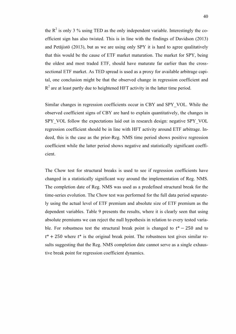
40
the R2 is only 3 % using TED as the only independent variable. Interestingly the co-
efficient sign has also twisted. This is in line with the findings of Davidson (2013)
and Petäjistö (2013), but as we are using only SPY it is hard to agree qualitatively
that this would be the cause of ETF market maturation. The market for SPY, being
the oldest and most traded ETF, should have maturate far earlier than the cross-
sectional ETF market. As TED spread is used as a proxy for available arbitrage capi-
tal, one conclusion might be that the observed change in regression coefficient and
R2 are at least partly due to heightened HFT activity in the latter time period.
Similar changes in regression coefficients occur in CBY and SPY_VOL. While the
observed coefficient signs of CBY are hard to explain quantitatively, the changes in
SPY_VOL follow the expectations laid out in research design: negative SPY_VOL
regression coefficient should be in line with HFT activity around ETF arbitrage. In-
deed, this is the case as the prior-Reg. NMS time period shows positive regression
coefficient while the latter period shows negative and statistically significant coeffi-
cient.
The Chow test for structural breaks is used to see if regression coefficients have
changed in a statistically significant way around the implementation of Reg. NMS.
The completion date of Reg. NMS was used as a predefined structural break for the
time-series evolution. The Chow test was performed for the full data period separate-
ly using the actual level of ETF premium and absolute size of ETF premium as the
dependent variables. Table 9 presents the results, where it is clearly seen that using
absolute premiums we can reject the null hypothesis in relation to every tested varia-
ble. For robustness test the structural break point is changed to and to
where is the original break point. The robustness test gives similar re-
sults suggesting that the Reg. NMS completion date cannot serve as a single exhaus-
tive break point for regression coefficient dynamics.
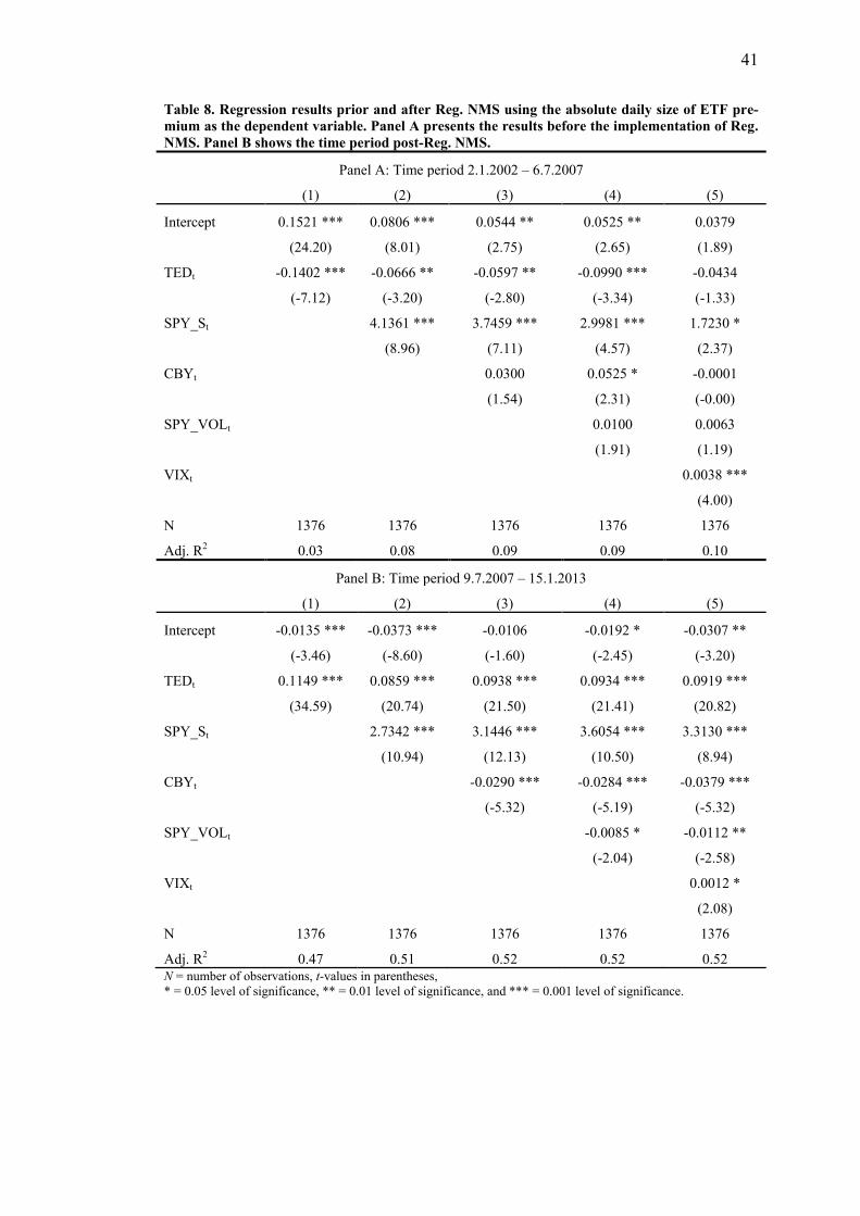
41
Table 8. Regression results prior and after Reg. NMS using the absolute daily size of ETF pre-
mium as the dependent variable. Panel A presents the results before the implementation of Reg.
NMS. Panel B shows the time period post-Reg. NMS.
Panel A: Time period 2.1.2002 – 6.7.2007
(1) (2) (3) (4) (5)
Intercept 0.1521 ***
(24.20)
0.0806 ***
(8.01)
0.0544 **
(2.75)
0.0525 **
(2.65)
0.0379
(1.89)
TEDt -0.1402 ***
(-7.12)
-0.0666 **
(-3.20)
-0.0597 **
(-2.80)
-0.0990 ***
(-3.34)
-0.0434
(-1.33)
SPY_St 4.1361 ***
(8.96)
3.7459 ***
(7.11)
2.9981 ***
(4.57)
1.7230 *
(2.37)
CBYt 0.0300
(1.54)
0.0525 *
(2.31)
-0.0001
(-0.00)
SPY_VOLt 0.0100
(1.91)
0.0063
(1.19)
VIXt 0.0038 ***
(4.00)
N 1376 1376 1376 1376 1376
Adj. R2 0.03 0.08 0.09 0.09 0.10
Panel B: Time period 9.7.2007 – 15.1.2013
(1) (2) (3) (4) (5)
Intercept -0.0135 ***
(-3.46)
-0.0373 ***
(-8.60)
-0.0106
(-1.60)
-0.0192 *
(-2.45)
-0.0307 **
(-3.20)
TEDt 0.1149 ***
(34.59)
0.0859 ***
(20.74)
0.0938 ***
(21.50)
0.0934 ***
(21.41)
0.0919 ***
(20.82)
SPY_St 2.7342 ***
(10.94)
3.1446 ***
(12.13)
3.6054 ***
(10.50)
3.3130 ***
(8.94)
CBYt -0.0290 ***
(-5.32)
-0.0284 ***
(-5.19)
-0.0379 ***
(-5.32)
SPY_VOLt -0.0085 *
(-2.04)
-0.0112 **
(-2.58)
VIXt 0.0012 *
(2.08)
N 1376 1376 1376 1376 1376
Adj. R2 0.47 0.51 0.52 0.52 0.52
N = number of observations, t-values in parentheses,
* = 0.05 level of significance, ** = 0.01 level of significance, and *** = 0.001 level of significance.

42
Table 9. The Chow test F-statistics using daily data and the most statistically and economically
relevant factors. F-statistics are reported using contemporaneous and 1-day lagged independent
variables. In panel A the dependent variable is the actual level of daily ETF premium. Panel B
presents the results using the absolute size of the ETF premium as the dependent variable. The
multivariate row presents the statistics using multivariate linear regressions with all statistically
significant factors.
Time period: 2.1.2002 – 15.1.2013 (Break point 9.7.2007)
Panel A:
Premium
Panel B:
abs(premium)
(t) (t-1) (t) (t-1)
Multivariate 5.4433 ***
(0.000)
2.4059 *
(0.025)
Multivariate 15.56 ***
(0.000)
12.69 ***
(0.000)
MONEY 11.23 ***
(0.000)
1.1973
(0.302)
TED 276.11 ***
(0.000)
267.02 ***
(0.000)
SPY_S 0.0291
(0.971)
3.4784 *
(0.031)
SPY_S 93.71 ***
(0.000)
85.62 ***
(0.000)
FH2 0.7491
(0.473)
1.0177
(0.362)
CBY 86.99 ***
(0.000)
83.75 ***
(0.000)
FH5 1.2253
(0.294)
0.9908
(0.371)
SPY_VOL 174.95 ***
(0.000)
163.26 ***
(0.000)
CBY 0.1457
(0.864)
0.1580
(0.854)
VIX 144.52 ***
(0.000)
134.16 ***
(0.000)
SPY_VOL 4.0298 *
(0.018)
8.1340 ***
(0.000)
N 2752 2752 N 2752 2752
N = number of observations, p-values in parentheses,
* = 0.05 level of significance, ** = 0.01 level of significance, and *** = 0.001 level of significance.
Rolling regression coefficients where estimated for more accurate analysis of the
relationship between dependent and independent variables. More importantly, this
methodology shows the possible change points in regression analysis dynamics. This
analysis is conducted to every independent variable revealing that all independent
variables and their relationship with absolute ETF premiums have experienced dra-
matic movements and changes in coefficient signs around the 2008 financial crisis.
The analysis shows that these changes occur two days prior the bankruptcy of Leh-
man Brothers, an investment bank, which triggered the most turbulent period of the
2008 financial crisis. This turbulent time in regression coefficients covers 50 trading
days.

43
In order to see if the implementation of Reg. NMS had potential effect on regression
coefficients, this 50-day period is removed from the time-series. Re-plotting the roll-
ing regression coefficients give smoother results showing that the only independent
variables with significant and persistent relationship with absolute size of ETF pre-
miums are TED spread and SPY_VOL. Appendix V shows the graphs with and
without the 50-day period of the financial crisis for every independent variable while
figure 1 presents the graphs for TED and SPY_VOL. The rolling regressions where
conducted using a 1376-day rolling window where the starting coefficient values
represent the coefficient from regressions run on the pre-Reg. NMS era (2.1.2002 –
6.7.2007). The plots end with the corresponding values from the regressions run on
the latter time period (9.7.2007 – 15.1.2013). The changes in coefficient signs hap-
pen to occur for both variables around the last phase of Reg. NMS. Similarly the ex-
planatory power measured as R2
rises steadily post-Reg. NMS. Although, by remov-
ing the financial crisis the betas and R2 values are roughly cut to half.
Figure 1. Rolling regression coefficients using TED and SPY_VOL. The dependent variable is
the absolute size of premiums. The period indicated by red lines in left figures is the 50-days
around Lehman Brothers bankruptcy while the period marked in red in the right side figures is
the starting point and completion of the last phase of Reg. NMS.
44
As the completion of Reg. NMS is expected to be a shock to the linear projection of
a dynamic system of ETF premiums (as is the financial crisis) we will use the
Kalman filter to estimate the time-varying betas of the two most significant factors
behind ETF premiums. Following this method we will reduce the noisiness to obtain
a statically more reliable estimate. In addition, using the Kalman filter algorithm to
obtain the beta estimates we will use the observed series to update the estimate to
learn from previous and new states of nature (see Kalman 1960; Grewal & Andrews
2008). Figure 2 presents the time-varying beta estimates for TED and SPY_VOL
using the Kalman filter method.
The figures show huge changes for both variables in time-varying beta estimates
during the period from mid-2007 to 2009. The beta estimate for TED has been rela-
tively close to zero during the whole period having experienced huge variation after
Reg. NMS and during the financial crisis. The SPY_VOL beta shows different be-
havior as its time-varying beta experienced a radical up-side movement from 2005 to
mid-2007 and falling rapidly after this point. This spiking point in time-varying
SPY_VOL beta coincides moderately with the completion of Reg. NMS. The ob-
served direction in beta estimate post-Reg. NMS has been falling. This might serve
as a proof that post-Reg. NMS period indeed has been having characteristically larg-
er trading volumes. The relationship with the rising trading volumes is inversely re-
lated to observed absolute size of ETF premiums, therefore leading to falling regres-
sion coefficient. This is in line with the argument that heightened HFT has some ef-
fects on ETF premiums by shrinking premiums efficiently via arbitrage process.
Moreover, the time-varying beta estimates show that most of the statistically signifi-
cant explanatory power of TED spread which is shown in linear regressions is due to
the short period during the financial crisis. One could argue that this verifies that
TED spread can explain ETF premiums during the times of high market stress but
has little statistical explanatory power to the actual level and sign of ETF premiums
outside of such periods. The connection to HFT is thus not as meaningful as ex-
plained in the research design and shown by the regression analysis. TED serves as a
proxy for market stress and can be used to predict ETF premiums in times of market
stress, when the normal arbitrage mechanism is distorted.
45
Figure 2. The time-varying betas using Kalman filters for TED and SPY_VOL as the independ-
ent variables and abs(ETF premium) as the dependent variable.
The results obtained by rolling regression analysis and Kalman filtered time-varying
beta estimation show outcomes which are partly in line with the expectations. It was
argued that TED spread as a proxy for arbitrage capital might be able to predict ETF
premiums. Our findings reveal that such an explanatory power largely appears as an
illusion in later times as it was only due to relatively small period during the financial
crisis. Still, in such times it can predict widening ETF premiums. Davidson (2013)
showed a relationship between prior stock market returns and daily ETF mispricing
while our results indicate that this is only due to 50-days around the financial crisis,
having very little meaning before that or in later times. Therefore this finding is
against prior cross-sectional16
empirical results.
In the research design we argued that prior levels of VIX can explain ETF premiums;
this is also related to heightened volatility during the financial crisis where the arbi-
trage mechanism supposedly broke down and has near zero explanatory power if this
era is removed. SPY_VOL on the other hand showed somewhat similar behavior as
was expected: its regression beta twisted during the period of Reg. NMS completion
and the factor has showed rising explanatory power since.
To see if this change in regression coefficient has been statistically significant, the
fluctuating process of the linear regression residuals was computed using recursive
16It is worth noting again that this study aims only to explain the premiums related to SPY, and not the
cross-sectional ETF universe.
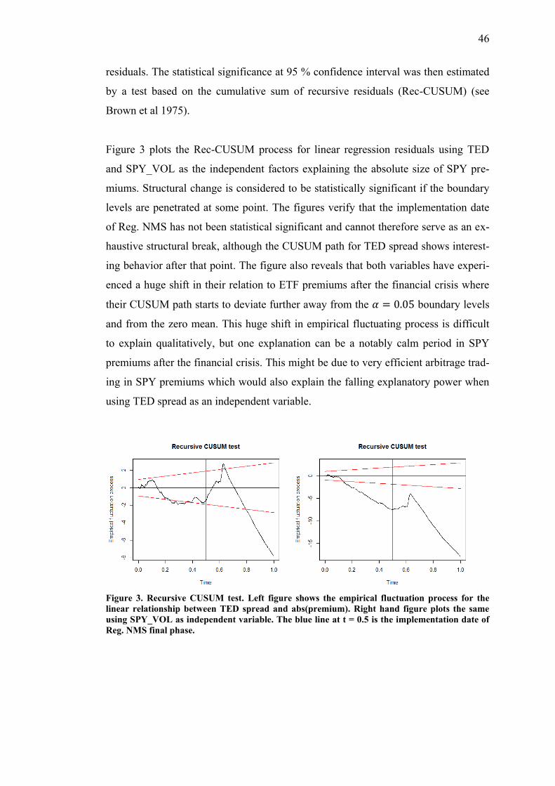
46
residuals. The statistical significance at 95 % confidence interval was then estimated
by a test based on the cumulative sum of recursive residuals (Rec-CUSUM) (see
Brown et al 1975).
Figure 3 plots the Rec-CUSUM process for linear regression residuals using TED
and SPY_VOL as the independent factors explaining the absolute size of SPY pre-
miums. Structural change is considered to be statistically significant if the boundary
levels are penetrated at some point. The figures verify that the implementation date
of Reg. NMS has not been statistical significant and cannot therefore serve as an ex-
haustive structural break, although the CUSUM path for TED spread shows interest-
ing behavior after that point. The figure also reveals that both variables have experi-
enced a huge shift in their relation to ETF premiums after the financial crisis where
their CUSUM path starts to deviate further away from the boundary levels
and from the zero mean. This huge shift in empirical fluctuating process is difficult
to explain qualitatively, but one explanation can be a notably calm period in SPY
premiums after the financial crisis. This might be due to very efficient arbitrage trad-
ing in SPY premiums which would also explain the falling explanatory power when
using TED spread as an independent variable.
Figure 3. Recursive CUSUM test. Left figure shows the empirical fluctuation process for the
linear relationship between TED spread and abs(premium). Right hand figure plots the same
using SPY_VOL as independent variable. The blue line at t = 0.5 is the implementation date of
Reg. NMS final phase.

47
8.3 ETF premium volatility modeling
The time period for ETF premium volatility modeling was chosen to represent the
characteristics of post-Reg. NMS era. The in-the-sample model specification period
is 09.07.2007 – 22.09.2011 (1051 observations) and the out-of-the-sample forecast-
ing and model testing period is 23.09.2011 – 31.10.2013 (525 observations).
The exogenous variables included to the modeling process were the most statistically
significant factors from the regression analysis in post-Reg. NMS era. Although
CBY was dropped out immediately as the observed relationship with ETF premiums
was qualitatively difficult to explain. After reviewing the GARCH model with possi-
ble candidates for exogenous variables, the chosen exogenous regressors are TED
spread and the feature scaled daily SPY trading volume (SPY_VOL). These factors
also have the most qualitatively meaningful role which follows tightly the research
design. They also proved to be the most statistically significant regressors measured
by their parameter standard errors.
The log series of daily SPY premiums shows significant autocorrelation. This was
aimed to be removed by modeling of the mean process. The ACF and PACF for the
AR(1) model residuals and squared residuals shows the existence of ARCH effects
on the time-series. GARCH(1,1) model specification was started with
ARMA(1,1)+GARCH(1,1) model including a list of exogenous variables. By drop-
ping out the insignificant variables and model parameters we obtained a simple
GARCH(1,1) with TED and SPY_VOL serving as exogenous variables in the vari-
ance equation while only TED showed statistical significance in the mean equation.
Models were also recalibrated using different distributions for the error terms: nor-
mal distribution, Student’s t-distribution, and skew Student’s t-distribution were test-
ed. The Student’s t-distribution proved to give the best fit for the time-series. The
final GARCH(1,1) with Student’s t-innovations and exogenous variables produced
the following model (table 10):
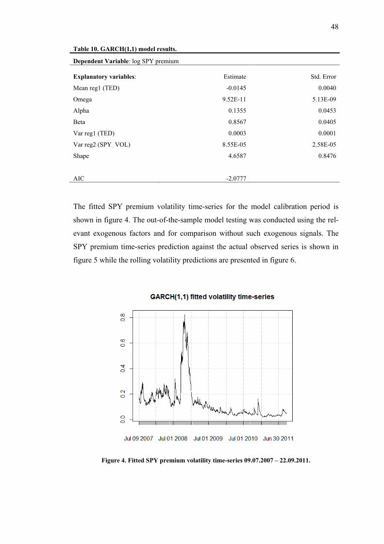
48
Table 10. GARCH(1,1) model results.
Dependent Variable: log SPY premium
Explanatory variables: Estimate Std. Error
Mean reg1 (TED) -0.0145 0.0040
Omega 9.52E-11 5.13E-09
Alpha 0.1355 0.0453
Beta 0.8567 0.0405
Var reg1 (TED) 0.0003 0.0001
Var reg2 (SPY_VOL) 8.55E-05 2.58E-05
Shape 4.6587 0.8476
AIC -2.0777
The fitted SPY premium volatility time-series for the model calibration period is
shown in figure 4. The out-of-the-sample model testing was conducted using the rel-
evant exogenous factors and for comparison without such exogenous signals. The
SPY premium time-series prediction against the actual observed series is shown in
figure 5 while the rolling volatility predictions are presented in figure 6.
Figure 4. Fitted SPY premium volatility time-series 09.07.2007 – 22.09.2011.
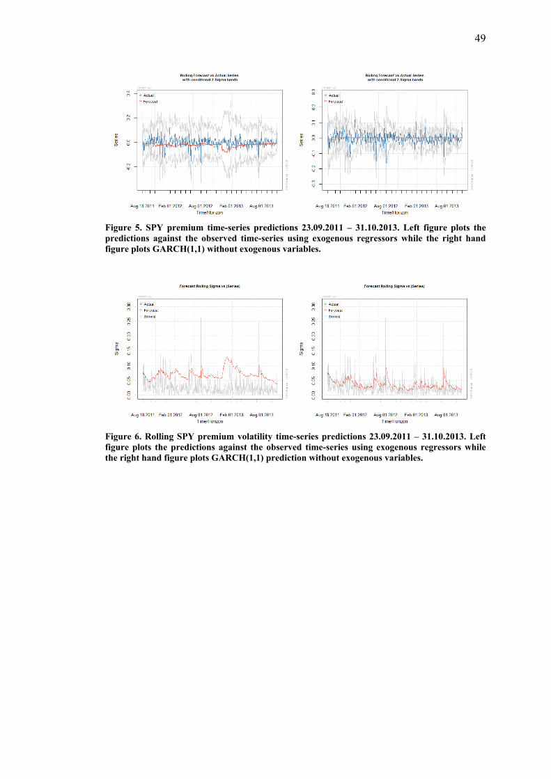
49
Figure 5. SPY premium time-series predictions 23.09.2011 – 31.10.2013. Left figure plots the
predictions against the observed time-series using exogenous regressors while the right hand
figure plots GARCH(1,1) without exogenous variables.
Figure 6. Rolling SPY premium volatility time-series predictions 23.09.2011 – 31.10.2013. Left
figure plots the predictions against the observed time-series using exogenous regressors while
the right hand figure plots GARCH(1,1) prediction without exogenous variables.
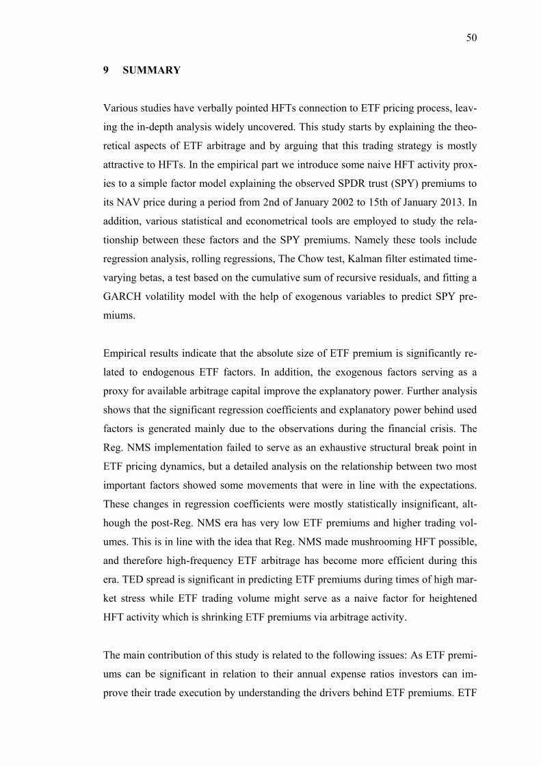
50
9 SUMMARY
Various studies have verbally pointed HFTs connection to ETF pricing process, leav-
ing the in-depth analysis widely uncovered. This study starts by explaining the theo-
retical aspects of ETF arbitrage and by arguing that this trading strategy is mostly
attractive to HFTs. In the empirical part we introduce some naive HFT activity prox-
ies to a simple factor model explaining the observed SPDR trust (SPY) premiums to
its NAV price during a period from 2nd of January 2002 to 15th of January 2013. In
addition, various statistical and econometrical tools are employed to study the rela-
tionship between these factors and the SPY premiums. Namely these tools include
regression analysis, rolling regressions, The Chow test, Kalman filter estimated time-
varying betas, a test based on the cumulative sum of recursive residuals, and fitting a
GARCH volatility model with the help of exogenous variables to predict SPY pre-
miums.
Empirical results indicate that the absolute size of ETF premium is significantly re-
lated to endogenous ETF factors. In addition, the exogenous factors serving as a
proxy for available arbitrage capital improve the explanatory power. Further analysis
shows that the significant regression coefficients and explanatory power behind used
factors is generated mainly due to the observations during the financial crisis. The
Reg. NMS implementation failed to serve as an exhaustive structural break point in
ETF pricing dynamics, but a detailed analysis on the relationship between two most
important factors showed some movements that were in line with the expectations.
These changes in regression coefficients were mostly statistically insignificant, alt-
hough the post-Reg. NMS era has very low ETF premiums and higher trading vol-
umes. This is in line with the idea that Reg. NMS made mushrooming HFT possible,
and therefore high-frequency ETF arbitrage has become more efficient during this
era. TED spread is significant in predicting ETF premiums during times of high mar-
ket stress while ETF trading volume might serve as a naive factor for heightened
HFT activity which is shrinking ETF premiums via arbitrage activity.
The main contribution of this study is related to the following issues: As ETF premi-
ums can be significant in relation to their annual expense ratios investors can im-
prove their trade execution by understanding the drivers behind ETF premiums. ETF

51
premium modeling can also be useful in risk management and in investment decision
making, while understanding HFTs’ role in ETF mispricing adds to our incomplete
knowledge on the effects of individual HFT strategies.

52
10 DISCUSSION
This study gets on with the research of individual HFT strategies and on their effects.
The empirical result interpretation is mainly related to the risk-profile of arbitrageurs.
The HFT activity around ETFs might be constrained by liquidity withdrawal, during
market crisis, and in other periods of high volatility. Relatively little is known of the
real HFT activity and how their trading behavior is related to factors such as used in
this study to proxy their activity, but one can argue that these factors represent HFT
risk-profiles at least in some level. There are times when HFT activity is reduced or
completely paused and this may lead to widening ETF premiums. In addition, the
high volatility and high cost of trading may cause HFTs to wait for a short amount of
time (e.g. a trading day) until the ETF premium widens even more. High cost to fi-
nance short-term trading activities may introduce risks and other limits of arbitrage
to arbitrageurs, making premiums last longer.
Previous studies have argued that TED spread as a proxy for arbitrage capital might
be able to predict ETF premiums. Our findings reveal that such an explanatory power
largely appears as an illusion in later times as it was only due to relatively small pe-
riod during the financial crisis. Still, in such times it can predict widening ETF pre-
miums. Davidson (2013) showed relationship between prior stock market returns and
daily cross-sectional ETF mispricing, while our results show that when concentrating
only to SPY this is due to 50-days during the financial crisis, having very little mean-
ing before that or in later times. Similarly, in the research design we argued in line
with previous papers that prior levels of VIX can explain ETF premiums. This is also
related to heightened volatility during the financial crisis where the arbitrage mecha-
nism supposedly broke down and has near zero explanatory power if this era is re-
moved. SPY_VOL on the other hand showed somewhat similar behavior as was ex-
pected: its regression beta twisted around the period of Reg. NMS completion and
the factor has showed rising explanatory power since.
The methodological choices used in this study leave a room for improvement. For
example, the ETF premium modeling process is overly simplistic and could be im-
proved by employing more sophisticated tools. This fundamental fragility is especial-
ly show in the chosen research data as we could only construct naive HFT proxies.
53
For example, ETF trade quotation data could be used to produce more reliable prox-
ies for HFT activity around a certain ETF. Furthermore, intraday data and trade iden-
tifiers could be used to construct tick-by-tick ETF trades to find out more accurately
the effects of HFT in ETF pricing process.
Even with it flaws, this study revealed various previously uncovered issues related to
the factors behind ETF mispricing. In addition, this was the first paper, to our
knowledge, to address the possible effects of Reg. NMS to ETF pricing process. The
paper can be useful in future research and especially for idea formation purposes.
Considering the current lack of empirical research on HFTs connection to ETF pric-
ing, further papers on the topic are extremely desirable and valuable.

54
REFERENCES
AFM=Authority for the Financial Markets (2010). High frequency trading: The
application of advanced trading technology in the European marketplace.
Available at: <http://www.afm.nl/~/media/files/rapport/2010/hft-report-
engels.ashx>. Cited 04.10.2013.
Aldridge, I. (2010). High-Frequency Trading: a Practical Guide to Algorithmic
Strategies and Trading Systems. New Jersey, John Wiley & Sons.
Angel, J., Harris, L. E. & Spatt, C. S. (2011). Equity trading in the 21st century.
Quarterly Journal of Finance 1(1), 1–53.
Avellaneda, M. & Stoikov, S. (2008). High-frequency trading in a limit order book.
Quantitative Finance 8(3), 217–224.
Baron, M., Brogaard, J. & Kirilenko, A. (2012). The trading profits of high frequency
traders. Available at: <http://ablealpha.com/Baron_Brogaard_Kirilenko
2012.pdf>. Cited 06.10.2012.
Ben-David, I., Franzoni, F. A. & Moussawi, R. (2012). ETFs, arbitrage, and shock
propagation. Swiss Finance Institute Research Paper No. 11-66. Available at:
<http://ssrn.com/abstract=1967599>. Cited 26.09.2013.
Benos, E. & Sagabe, S. (2012). High-frequency trading behaviour and its impacy on
market quality: evidence from the UK equity market. Bank of England Working
Paper No. 469.
Biais, B. & Woolley, P. (2012). The flip side: high frequency trading. Financial
World, February 2012. Available at: <http://www.lse.ac.uk/fmg/research
Programmes/paulWoolleyCentre/pdf/FinancialWorldArticle.pdf >. Cited
06.10.2013.
Biais, B., Foucault, T. & Moinas, S. (2013). Equilibrium fast trading. SSRN Working
Paper No. 2024360. Available at: <http://ssrn.com/abstract=2024360>. Cited
02.10.2013.
Blackrock (2011). ETF Landscape – Industry Review, 2011 – H1.
Bloomberg (2013). China trading error shakes confidence in world’s worst equities.
Bloomberg News 16.08.2013. Available at <http://www.businessweek.com
/news/2013-08-16/china-shanghai-composite-surges-as-exchange-said-to-
investigate>. Cited 29.09.2013.
Bollerslev, T., Engle, R. F. & Nelson, D. B. (1994). ARCH model. In: Engle, R. F. &
McFadden, D. C. (ed.). Handbook of Econometrics IV, 2959–3038.
Amsterdam, Elsevier Science.
55
Borkovec, M., Domowitz, I., Serbin, V. & Yegerman, H. (2010). Liquidity and price
discovery in exchange-traded funds: One of several possible lessons from the
Flash Crash. Investment Technology Group Paper, May 2010. Available at:
<http://www.itg.com/news_events/ITG-Paper-LiquidityPriceDiscovery.pdf>.
Cited 01.10.2013.
Bradley, H. & Litan, R. E. (2011). ETFs and the present danger to capital formation.
Ewing Marion Kauffman Foundation Research Paper. Available at:
<http://ssrn.com/abstract=1947346>. Cited 01.10.2013.
Brogaard, J. (2010). High frequency trading and its impact on market quality.
SSRN Working Paper No. 1641387. Available at: <http://ssrn.com/
abstract=1641387>. Cited 25.9.2013.
Brogaard, J., Hendershott, T. & Riordan, R. (2013a). High frequency trading and
price discovery. SSRN Working Paper No. 1928510. Available at:
<http://ssrn.com/abstract=1928510>. Cited 01.10.2013.
Brogaard, J., Hendershott, T., Hunt, S., Latza, T., Pedace, L. & Ysusi, C. (2013b).
High-frequency trading and the execution costs of institutional investors. FSA
Occasional Paper Series No. 43.
Brooks, C. (2002). Introductory econometrics for finance. Cambridge: University
Press
Brown, R. L., Durbin, J. & Evans, J. M. (1975). Techniques for testing the constancy
of regression relationships over time. Journal of the Royal Statistical Society B
37, 149–163.
Brown, S., Lynch, A. & Petäjistö, A. (2010). Hedge funds, mutual funds, and ETFs.
In: Archarya et al. (ed.). Regulating Wall Street: The Dodd-Frank act and the
New Architecture of Global Finance, 351–366.
Brownlees, C. T., Cipollini, F. & Gallo, G. M. (2011). Intra-daily volume modeling
and prediction for algorithmic trading. Journal of Financial Econometrics 9(3),
489–518.
Brunnermeier, M.K., Nagel, S. & Pedersen, L. (2009). Carry trades and currency
crashes. NBER Macroeconomics Annual 23, 313–347.
Cartea, A. & Penalva, J. (2012). Where is the value in high frequency trading?
Quarterly Journal of Finance 2(3), 1–46.
Cartea, A. & Jaimungal, S. (2013). Risk metrics and fine tuning of high-frequency
trading strategies. Mathematical Finance, in press. Available at:
<http://ssrn.com/abstract=2010417>. Cited 02.10.2013.

56
CESR=Committee of European Securities Regulators. (2010). CESR technical
advice to the European Commission in the context of the MiFID review and
responses to the European Commission request for additional information.
Available at: <http://www.esma.europa.eu/system/files/Compiled_version_
Technical_Advice_and_Additional_Information_MiFID_Review.pdf>.
Cited 25.09.2013.
CFTC-SEC. (2010). Findings regarding the market events of May 6, 2010. Available
at: <http://www.sec.gov/spotlight/sec-cftcjointcommittee.shtml>. Cited
25.09.2013.
Chaboud, A., Chiquoine, B., Hjalmarsson, E. & Vega, C. (2009). Rise of the
machines: algorithmic trading in the foreign exchange market. FED
International Finance Discussion Paper No 980. Available at:
<http://www.federalreserve.gov/pubs/ifdp/2009/980/ifdp980.pdf>. Cited
25.09.2013.
Chan, E. P. (2013). Algorithmic Trading: Winning Strategies and Their Rationale.
John Wiley & Sons, Hoboken NJ.
Chen, W-P., Chou, R. & Chung, H. (2008). Decimalization and the ETFs and futures
pricing efficiency. Journal of Futures Markets 29(2), 157–178.
Chordia, T., Roll, R. & Subrahmanyam, A. (2011). Recent trends in trading activity
and market quality. Journal of Financial Economics 101(2), 243–263.
Chow, G. (1960). Test of equality between sets of coefficients in two linear
regressions. Econometrica 28(3), 591–605.
Cohen, S. N. & Szpruch, L. (2012). A limit order book model for latency arbitrage.
Mathematics and Financial Economics 6(3), 211–227.
Creswell, J. (2010). Speedy new traders make waves far from Wall Street. New
York Times. Available at: <http://www.nytimes.com/2010/05/17/
business/17trade.html?dbk> Cited 25.9.2013.
Cvitanic, J. & Kirilenko, A. (2010). High frequency traders and asset prices. SSRN
Working Paper No. 1569075. Available at: <http://ssrn.com/
abstract=1569075>. Cited 25.09.2013.
Davidson, L. (2013). Examining the exchange-traded nature of exchange-traded
funds. Morningstar ETF Research 11.02.2013. Available at:
<https://corporate.morningstar.com/us/documents/MethodologyDocuments/
ResearchPapers/exchangetradednature.pdf>. Cited 30.09.2013.
Deutsche Bank (2013). Synthetic equity & index strategy: 2012 ETF review & 2013
outlook. Deutsche Bank Market Research 11.01.2013.
57
Easley, D., López de Prado, M. & O'Hara, M. (2011). The microstructure of the
'Flash Crash': flow toxicity, liquidity crashes and the probability of informed
trading. The Journal of Portfolio Management 37(2), 118–128.
Easthope, D. & Lee, C. (2009). Demystifying and evaluating high frequency
equities trading. Fast forward or pause? Celent Reports. Available at:
<http://www.celent.com/reports/demystifying-and-evaluating-high-frequency-
equities-trading-fast-forward-or-pause>. Cited 25.09.2013.
Engle, R. (1982). Autoregressive conditional heteroskedasticity with estimates of the
variance of U.K. inflation. Econometrica 45, 987–1007.
Engle, R. & Sarkar, D. (2002). Pricing exchange traded funds. NYU Working Paper
No. S-DRP-02-11. Available at: <http://ssrn.com/abstract=1296379>. Cited
30.09.2013.
Engle, R. & Sarkar, D. (2006). Premiums-discounts and exchange-traded funds.
Journal of Derivatives 13(4), 27–45.
Fabozzi, F. J., Kolm, P. N., Pachamanova, D. & Focardi, S. (2007). Robust portfolio
Optimization and Management. John Wiley & Sons, Hoboken NJ.
Fabozzi, F. J., Focardi, S. M. & Jonas, C. (2011). High-frequency trading:
methodologies and market impact. Review of Futures Markets 9, 7–38.
Gallagher, D. & Segara, R. (2005). The performance and trading characteristics of
exchange-traded funds. Journal of Investment Strategy 1(1), 47–58.
Garvey, R. & Wu, F. (2010). Speed, distance, and electronic trading: new evidence
on why location matters. Journal of Financial Markets 13, 367–396.
Gastineau, G. L. (2008). Exchange-Traded Funds. Handbook of Finance. John
Wiley & Sons, Hoboken NJ.
Golub, A., Keane, J. & Poon. S-H. (2012). High frequency trading and mini flash
crashes. SSRN Working Paper No. 2182097. Available at: <http://ssrn.com
/abstract=2182097>. Cited 08.10.2013.
Gomber, P., Arndt, B,, Lutat, M. & Uhle, T. (2011). High-frequency trading. SSRN
Working Paper No. 1858626. Available at: <http://ssrn.com/abstract
=1858626>. Cited 25.09.2013.
GOS=the Government Office for Science, UK. (2012). Foresight: the future of
computer trading in financial markets. The Government Office for Science,
London. Available at: <http://www.bis.gov.uk/assets/foresight/docs/computer-
trading/12-1086-future-of-computer-trading-in-financial-markets-report.pdf>.
Cited 07.10.2013.
Grewal, M. & Andrews, A. (2008). Kalman Filtering – Theory and Practice Using
MATLAB. 3rd
Edition. Wiley & Sons, Hoboken, NJ.

58
Guilbaud, F. & Pham, H. (2013). Optimal high-frequency trading with limit and
market orders. Quantitative Finance 13(1), 79–94.
Hagströmer, B. & Nordén, L. (2013). The diversity of high-frequency traders. SSRN
Working Paper No. 1858626. Available at: <http://ssrn.com/abstract=
1858626>. Cited 02.10.2013.
Hasbrouck, J. (2007). Empirical Market Microstructure: The Institutions, Economics,
and Econometrics of Securities Trading. Oxford University Press.
Hasbrouck, J. & Saar, G. (2013). Low-latency trading. Journal of Financial Markets,
in press. Available at: <http://www.sciencedirect.com/science/article/pii/
S1386418113000165>. Cited 25.09.2013.
Hendershott, T., Jones, C. & Menkveld, A. (2011). Does algorithmic trading
improve liquidity? Journal of Finance 66(1), 1–33.
Hendershott, T. & Moulton, P. C. (2011). Automation, speed and market quality: The
NYSE Hybrid. Journal of Financial Markets 14, 568–604.
Hendershott, T. & Riordan, R. (2011). Algorithmic trading and information. NET
Institute Working Paper No. 09-08. Available at: <http://econpapers.repec.org
/paper/netwpaper/0908.htm>. Cited 25.9.2013.
Jares, E. T. & Lavin, A. M. (2004). Japan and Hong-Kong exchange-traded funds
(ETFs): discounts, returns, and trading strategies. Journal of Financial Service
Research 25(1), 57–69.
Jarrow, R. A. & Protter, P. (2012). A dysfunctional role of high frequency trading
in electronic markets. International Journal of Theoretical and Applied
Finance 15(3), 79–94.
Jones, C. M. (2013). What do we know about high-frequency trading? Columbia
Business School Research Papers No. 13-11. Available at: <http://ssrn.com/
abstract=2236201>. Cited 07.10.2013
Jovanovic, B. & Menkveld, A. (2010). Middlemen in limit-order markets. Western
Finance Association (WFA), 2011. Available at: <http://ssrn.com/
abstract=1624329>. Cited 25.09.2013.
Kalman, R. E. (1960). A new approach to linear filtering and prediction problems.
Journal of Basic Engineering 82 D, 35–45.
Kearns, M., Kulesza, A. & Nevmyvaka, Y. (2010). Empirical limitations on high
frequency trading profitability. SSRN Working Paper No. 1678758. Available
at: <http://ssrn.com/abstract=1678758>. Cited 25.09.2013.
Kim, S. & Murphy, D. (2013). The impact of high-frequency trading on stock market
liquidity measures. SSRN Working Paper No. 2278428. Available at:
<http://ssrn.com/abstract=2278428>. Cited 10.10.2013.
59
Kirilenko, A., Kyle, A., Samadi, M. & Tuzun, T. (2011). The Flash Crash: the
impact of high frequency trading on an electronic market. SSRN Working
Paper No. 1686004. Available at: <http://ssrn.com/abstract=1686004>.
Cited 25.09.2013.
Kosev, M. & Williams, T. (2011). Exchange-traded funds. Reserve Bank of Australia.
Available at: <http://www.rba.gov.au/publications/bulletin/2011/mar/pdf/bu-
0311-8.pdf>. Cited 04.10.2013.
Krudy, E. (2010). Is the May 6 “Flash Crash” in US stock markets the new normal?
Reuters. Available at: <www.reuters.com/article/idUSN1057063420100610>.
Cited 25.9.2013.
LSE=London Stock Exchange. (2012a). Direct market access. Available at:
<http://www.londonstockexchange.com/prices-and-markets/stocks/tools-and-
services/direct-market-access/direct-market-access.htm>. Cited 25.09.2013.
LSE=London Stock Exchange. (2012b). Sponsored access. Available at:
<http://www.londonstockexchange.com/products-and-services/trading-
services/sponsored-access/sponsored-access.htm>. Cited 25.09.2013.
Madhavan, A. (2012). Exchange-traded funds, market structure and the Flash Crash.
SSRN Working Paper No. 1932925. Available at:
<http://ssrn.com/abstract=1932925 >. Cited 01.10.2013.
Marshall, B., Nguyen, N. H. & Visaltanachoti, N. (2010). ETF arbitrage: intraday
evidence. SSRN Working Paper No. 1709599. Available at:
<http://ssrn.com/abstract= 1709599>. Cited 29.09.2013.
Menkveld, A. (2013). High frequency trading and the new-market makers. SSRN
Working Paper No. 1722924. Available at: <http://ssrn.com/abstract
=1722924>. Cited 25.09.2013.
Milonas, N. & Rompotis, G. (2006). Investigating European ETFs: the case of the
Swiss exchange traded funds. HFAA Annual Conference Paper. Available at:
<http://www.efmaefm.org/0EFMAMEETINGS/EFMA%20ANNUAL%20ME
ETINGS/2007-Vienna/Papers/0232.pdf>. Cited 10.10.2013.
Nanex (2012). Citigroup Micro-Crash. Available at <http://www.nanex.net/
aqck2/3550.html>. Cited 29.09.2013.
Narang, M. (2010). Tradeworx Inc. public commentary on SEC market structure
concept release. Comments on concept release on equity market structure.
Available at: <http://www.sec.gov/comments/s7-02-10/s70210-129.pdf>.
Cited 25.09.2013.
Noble, J. (2013). Computer error blamed in Everbright trading mishap. The
Financial Times 19.08.2013. Available at
<http://www.ft.com/intl/cms/s/0/9885f876-0880-11e3-badc-
00144feabdc0.html?siteedition=intl#axzz2cPVi52r1>. Cited 29.09.2013.
60
Pagnotta, E. & Philippon, T. (2012). Competing on speed. SSRN Working Paper No.
1967156. Available at: <http://ssrn.com/ abstract=1967156>. Cited 04.10.2013.
Petäjistö, A. (2011). Characteristics of Market Trading in Exchange-Traded Funds:
2009–2010. NYU Stern School of Business. Available at:
<http://www.petajisto.net/papers/etfev15.pdf>. Cited 25.09.2013.
Petäjistö, A. (2013). Inefficiencies in the pricing of exchange-traded funds. SSRN
Working Paper No. 2000336. Available at: <http://ssrn.com/ abstract=
2000336>. Cited 30.9.2013.
Philips, M. (2012). Knight shows how to lose $440 million in 30 minutes. Bloomberg
Businessweek 02.08.2013. Available at <http://www.businessweek.com/
articles/2012-08-02/knight-shows-how-to-lose-440-million-in-30-minutes>.
Cited 29.09.2013.
Prix, J., Loist, O. & Huetl, M. (2007). Algorithmic trading patterns in Xetra orders.
The European Journal of Finance 13(8), 717–739.
Ramaswamy, S. (2011). Market structures and systemic risks of exchange-traded
funds. BIS Working Papers No. 343. Available at: <http://www.bis.org/
publ/work343.pdf>. Cited 01.10.2013.
Reverre, S. (2001). The Complete Arbitrage Deskbook. McGraw-Hill, New York.
Richie, N., Daigler, R. T. & Gleason, K. C. (2008). The limits to stock index
arbitrage: examining S&P 500 futures and SPDRs. Journal of Futures Markets
28(12), 1182–1205.
Riordan, R. & Storkenmaier, A. (2012). Latency, liquidity and price discovery.
Journal of Financial Markets 15, 416–437.
Saario, J. (2011). Robottikauppa ottaa ohjat. Kauppalehti 14.10.2011: 14-15.
SEC=Securities and Exchange Commission (2007). Regulation NMS Compliance
Date Extension. Available at: <http://www.sec.gov/rules/final/2007/34-
55160.pdf>. Cited 19.11.2013.
SEC=Securities and Exchange Commission (2010). Concept release on equity
market structure. Available at: <http://www.sec.gov/rules/concept/2010/34-
61358.pdf>. Cited 02.10.2013.
Sharpe, W. & Alexander, G. (1990). Investments. 4th
edition. Prentice and Hall, N. J.
Shleifer, A. & Vishny, R.W. (1997). The limits of arbitrage. Journal of Finance 52,
35–55.
Smith, R. (2010). Is high-frequency trading inducing changes in market
microstructure and dynamics? SSRN Working Paper No. 1632077. Available
at: <http://ssrn.com/abstract=1632077>. Cited 27.09.2013.
61
Sornette, D. & von der Becke, S. (2011). Crashes and high frequency trading: an
evaluation of risks posed by high-speed algorithmic trading. Swiss Finance
Institute Research Paper No. 11-63.
The Economist. (2013a). Electronic trading: Dutch fleet. The Economist 20.04.2013:
66.
The Economist (2013b). Exchange-traded funds: twenty years young. The Economist
26.01.2013.
Trainor, W. (2010). Do leveraged ETFs increase volatility? Technology and
Investment 1(3), 215–220.
Tsay, R. S. (2005). Analysis of Financial Time Series (2nd
edition). John Wiley &
Sons, Hoboken, NJ.
Wah, E. & Wellman, M. P. (2013). Latency arbitrage, market fragmentation, and
efficiency: a two-market model. Proceedings of the 14th ACM Conference on
Electronic Commerce. Available at: <http://web.eecs.umich.edu/srg/wp-
content/uploads/2013/02/twomarketmodel.pdf>. Cited 03.10.2013.
Zhang, F. (2010). High-frequency trading, stock volatility and price discovery.
SSRN Working Paper No. 1691679. Available at: <http://ssrn.com/ ab-
stract=1691679>. Cited 25.9.2013.
62
APPENDICES
Appendix I List of factors and data sources
Available Arbitrageurs Capital:
TED Spread (TED) is defined as the difference between 3-month LIBOR and T-bill
rates. Brunnermeier et al. (2009) explain the importance of TED spread as a premium
that financial institutions would have to pay for their lending to finance their trading
activities in relation to the true risk-free rate.
Source: http://www.federalreserve.gov/releases/h15/data.htm.
VIX Index (VIX) is defined as the Chicago Board Options Exchange Market Volatili-
ty Index. This serves as a proxy for available arbitrageurs’ capital as higher volatility
increases traders capital needs. Petäjistö (2011) and Davidson (2013) have docu-
mented the significance between VIX levels and ETF premiums. Source:
http://finance.yahoo.com/q?s=^VIX.
Bond-oriented Risk Factors:
Yield Spread (YSPR) is defined as the difference between Moody’s seasoned Baa
corporate bond yield (BAA) and 10-year Treasury constant maturity rate (GS10).
Source: http://www.federalreserve.gov/releases/h15/data.htm.
Corporate Bond Yield (CBY) is the difference between Moody’s seasoned Baa cor-
porate bond yield (BAA) and Moody’s seasoned Aaa corporate bond yield (AAA).
Source: http://www.federalreserve.gov/releases/h15/data.htm.
Fung-Hsieh Mutual Fund Risk Factors applicable at daily level:
FH1: US Equities: MSCI North American Equities [Datastream series:
MSUSAM$(RI)].
FH2: Non-US Equities: MSCI non-US Equities [Datastream series: MSWXUS$(RI)].
63
FH3: Emerging Market Equities: MSCI Emerging Market index monthly total return
[Datastream series: MSEMKF$(RI)].
FH4: 1-month Eurodollar Deposit Return: One-month Eurodollar deposit rate of the
previous month [Datastream series: ECUSD1M].
FH5: Spot Gold: Unofficial price for spot gold London morning fixing [Datastream
series: GOLDBLN(UF)].
Source for above factors: THOMSON REUTERS DATASTREAM.
FH6: TWEXMMTH: Trade Weighted U.S. Dollar Index. Source:
http://www.federalreserve.gov/releases/h10/Summary/indexn96_b.txt.
Kenneth French Industry Portfolios (Financial Industry Stress Factor):
Finance Industry Portfolio (MONEY). Finance industry value weighted returns.
Source: http://mba.tuck.dartmouth.edu/pages/faculty/ken.french/data_library.html.
ETF Endogenous Factors (HFT activity proxies):
Daily SPY volatility (SPY_S). A simple estimation of daily volatility calculated by
using the true range of daily price variation. This is calculated as follows:
where is the highest price during day t, is the lowest price in day t, and
is the closing price at day t. Source: Bloomberg.
SPY trading volume (SPY_VOL). A standardized measure of ETF daily trading vol-
ume with mean 0 and standard deviation of 1. A high daily value, say above one
sigma, indicates higher than normal trading volume. This can serve as a simple proxy
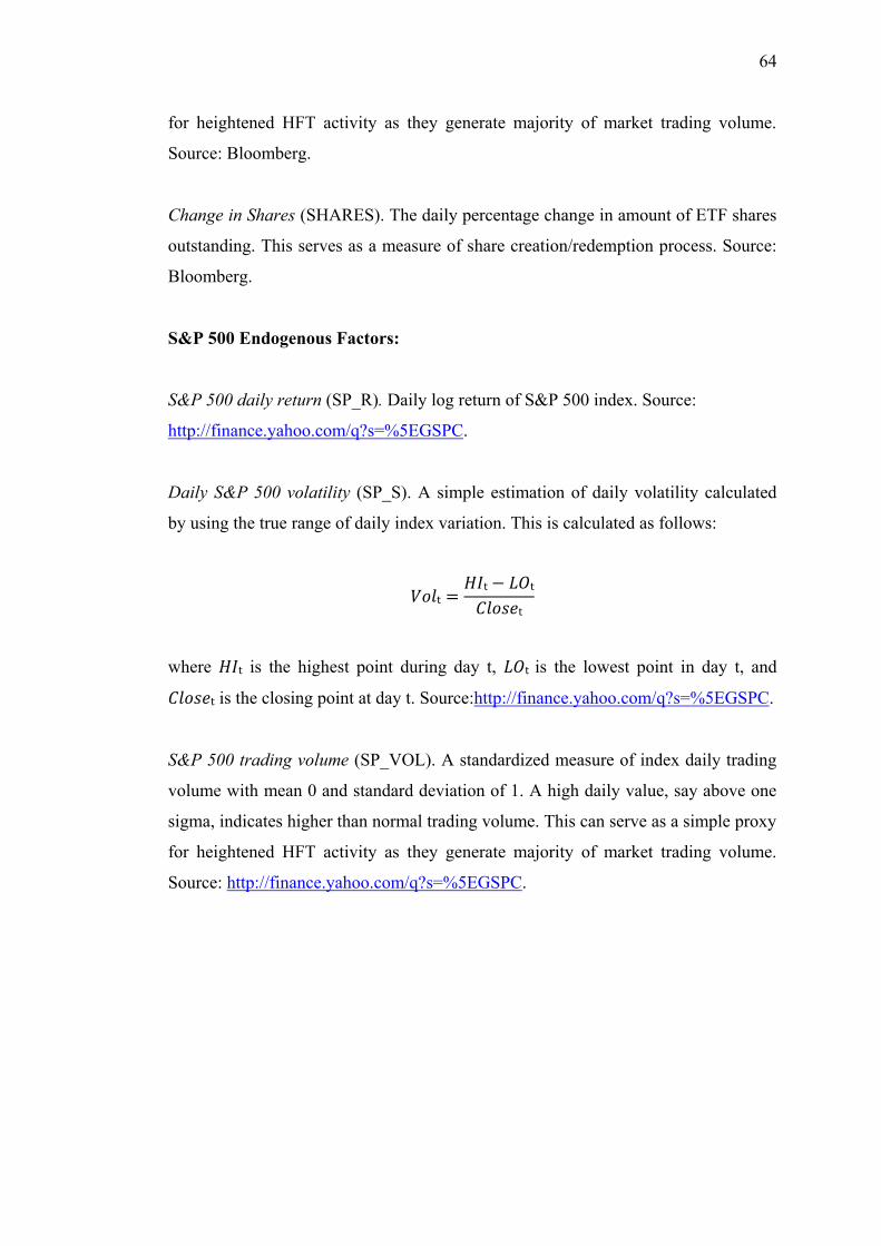
64
for heightened HFT activity as they generate majority of market trading volume.
Source: Bloomberg.
Change in Shares (SHARES). The daily percentage change in amount of ETF shares
outstanding. This serves as a measure of share creation/redemption process. Source:
Bloomberg.
S&P 500 Endogenous Factors:
S&P 500 daily return (SP_R). Daily log return of S&P 500 index. Source:
http://finance.yahoo.com/q?s=%5EGSPC.
Daily S&P 500 volatility (SP_S). A simple estimation of daily volatility calculated
by using the true range of daily index variation. This is calculated as follows:
where is the highest point during day t, is the lowest point in day t, and
is the closing point at day t. Source:http://finance.yahoo.com/q?s=%5EGSPC.
S&P 500 trading volume (SP_VOL). A standardized measure of index daily trading
volume with mean 0 and standard deviation of 1. A high daily value, say above one
sigma, indicates higher than normal trading volume. This can serve as a simple proxy
for heightened HFT activity as they generate majority of market trading volume.
Source: http://finance.yahoo.com/q?s=%5EGSPC.
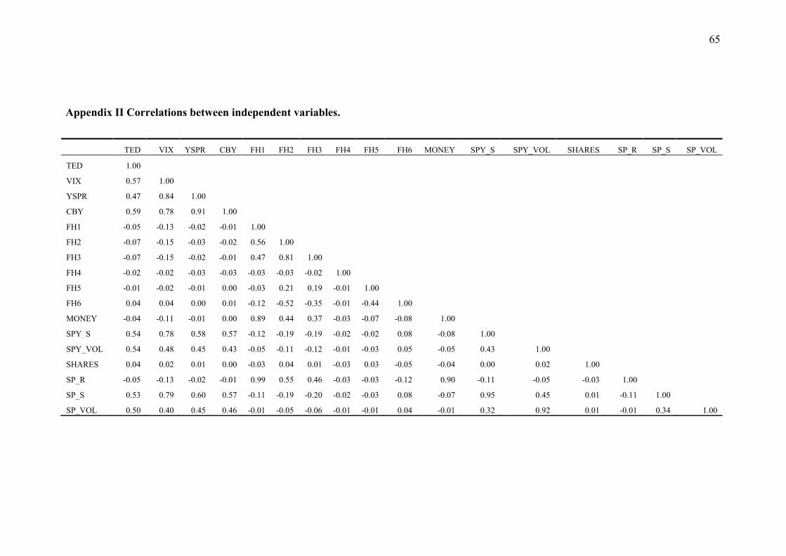
65
Appendix II Correlations between independent variables.
TED VIX YSPR CBY FH1 FH2 FH3 FH4 FH5 FH6 MONEY SPY_S SPY_VOL SHARES SP_R SP_S SP_VOL
TED 1.00
VIX 0.57 1.00
YSPR 0.47 0.84 1.00
CBY 0.59 0.78 0.91 1.00
FH1 -0.05 -0.13 -0.02 -0.01 1.00
FH2 -0.07 -0.15 -0.03 -0.02 0.56 1.00
FH3 -0.07 -0.15 -0.02 -0.01 0.47 0.81 1.00
FH4 -0.02 -0.02 -0.03 -0.03 -0.03 -0.03 -0.02 1.00
FH5 -0.01 -0.02 -0.01 0.00 -0.03 0.21 0.19 -0.01 1.00
FH6 0.04 0.04 0.00 0.01 -0.12 -0.52 -0.35 -0.01 -0.44 1.00
MONEY -0.04 -0.11 -0.01 0.00 0.89 0.44 0.37 -0.03 -0.07 -0.08 1.00
SPY_S 0.54 0.78 0.58 0.57 -0.12 -0.19 -0.19 -0.02 -0.02 0.08 -0.08 1.00
SPY_VOL 0.54 0.48 0.45 0.43 -0.05 -0.11 -0.12 -0.01 -0.03 0.05 -0.05 0.43 1.00
SHARES 0.04 0.02 0.01 0.00 -0.03 0.04 0.01 -0.03 0.03 -0.05 -0.04 0.00 0.02 1.00
SP_R -0.05 -0.13 -0.02 -0.01 0.99 0.55 0.46 -0.03 -0.03 -0.12 0.90 -0.11 -0.05 -0.03 1.00
SP_S 0.53 0.79 0.60 0.57 -0.11 -0.19 -0.20 -0.02 -0.03 0.08 -0.07 0.95 0.45 0.01 -0.11 1.00
SP_VOL 0.50 0.40 0.45 0.46 -0.01 -0.05 -0.06 -0.01 -0.01 0.04 -0.01 0.32 0.92 0.01 -0.01 0.34 1.00
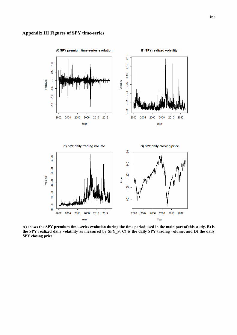
66
Appendix III Figures of SPY time-series
A) shows the SPY premium time-series evolution during the time period used in the main part of this study. B) is
the SPY realized daily volatility as measured by SPY_S. C) is the daily SPY trading volume, and D) the daily
SPY closing price.

67
Appendix IV Regression results prior and after Reg. NMS
Regression results using actual level of premiums with divided time period. The dependent variable is the daily
ETF premium. Panel A presents the results before the implementation of Reg. NMS. Panel B shows the time
period post-Reg. NMS. Independent variables are dropped according to lowest absolute t-statistics from the
regression run to the latter time period (2007-2013).
Panel A: Time period 2.1.2002 – 6.7.2007
(1) (2) (3) (4)
Intercept -0.0035
(-0.75)
0.0205 *
(2.34)
0.0210 *
(2.38)
0.0209 *
(2.36)
MONEYt 0.0027
(0.62)
0.0023
(0.52)
0.0033
(0.68)
0.0037
(0.74)
SPY_St -1.9142 **
(-3.20)
-1.9512 **
(-3.23)
-1.9478 **
(-3.23)
FH2t -0.2745
(-0.48)
-0.3350
(-0.56)
FH5t 0.1602
(0.34)
N 1376 1376 1376 1376
Adj. R2 0.00 0.01 0.01 0.01
Panel B: Time period 9.7.2007 – 15.1.2013
(1) (2) (3) (4)
Intercept -0.0113 **
(-2.68)
0.0267 ***
(4.02)
0.0217 **
(3.27)
0.0218 ***
(3.31)
MONEYt -0.0179 ***
(-10.86)
-0.0190 ***
(-11.69)
-0.0232 ***
(-12.94)
-0.0245 ***
(-13.51)
SPY_St -2.1844 ***
(-7.34)
-1.8793 ***
(-6.26)
-1.8372 ***
(-6.15)
FH2t 1.5907 ***
(5.33)
1.9220 ***
(6.22)
FH5t -1.2028 ***
(-3.89)
N 1376 1376 1376 1376
Adj. R2 0.08 0.11 0.13 0.14
N = number of observations, t-values in parentheses,
* = 0.05 level of significance, ** = 0.01 level of significance, and *** = 0.001 level of significance.

68
Appendix V Figures of rolling regression coefficients
The rolling regression coefficients for the rest of the independent variables using abs(ETF premium) as the de-
pendent variable. The period indicated by red lines in left figures is the 50-days around Lehman Brothers bank-
ruptcy while the period marked in red in the right side figures is the starting point and completion of the last
phase of Reg. NMS.
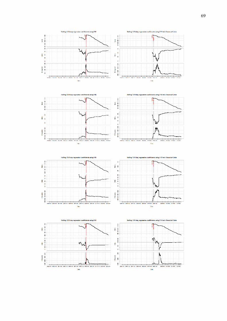
69
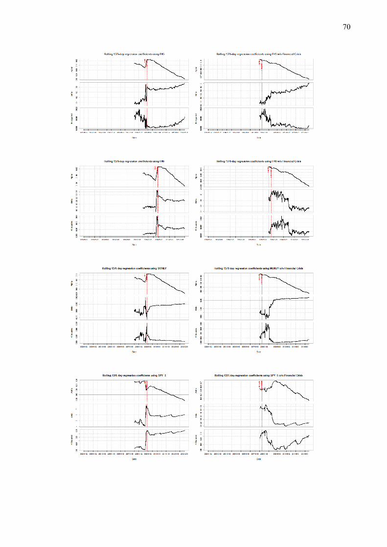
70
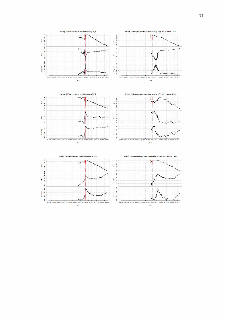
71