Origin choice and petal loss in the flower garden of spiral wave tip trajectoriesRichard A. Gray, John P. Wikswo, and Niels F. Otani Citation: Chaos: An Interdisciplinary Journal of Nonlinear Science 19, 033118 (2009); doi: 10.1063/1.3204256 View online: http://dx.doi.org/10.1063/1.3204256 View Table of Contents: http://scitation.aip.org/content/aip/journal/chaos/19/3?ver=pdfcov Published by the AIP Publishing Articles you may be interested in Non-specular reflections in a macroscopic system with wave-particle duality: Spiral waves in bounded media Chaos 23, 013134 (2013); 10.1063/1.4793783 Soliton ratchets in homogeneous nonlinear Klein-Gordon systems Chaos 16, 013117 (2006); 10.1063/1.2158261 The Lund–Regge surface and its motion’s evolution equation J. Math. Phys. 43, 1938 (2002); 10.1063/1.1452776 Parametrically forced pattern formation Chaos 11, 52 (2001); 10.1063/1.1350454 Dynamics of a nonlinear parametrically excited partial differential equation Chaos 9, 242 (1999); 10.1063/1.166397

This article is copyrighted as indicated in the article. Reuse of AIP content is subject to the terms at: http://scitation.aip.org/termsconditions. Downloaded to IP:

209.183.185.254 On: Sun, 30 Nov 2014 01:13:33

Origin choice and petal loss in the flower garden of spiral wave tiptrajectories

Richard A. Gray,1,a� John P. Wikswo,2 and Niels F. Otani31Division of Physics, Office of Science and Engineering Laboratories, Center for Devices and RadiologicalHealth, Food and Drug Administration, Silver Spring, Maryland 20993, USA and Department ofBiomedical Engineering, University of Alabama at Birmingham, Birmingham, Alabama 35294, USA2Departments of Biomedical Engineering, Molecular Physiology and Biophysics, and Physics and Astronomy,Vanderbilt Institute for Integrative Biosystems Research and Education, Vanderbilt University, Nashville,Tennessee 37235, USA3Department of Biomedical Sciences, Veterinary Research Tower, Cornell University, Ithaca,New York 14853-6401, USA

�Received 12 November 2008; accepted 22 July 2009; published online 14 August 2009�

Rotating spiral waves have been observed in numerous biological and physical systems. Thesespiral waves can be stationary, meander, or even degenerate into multiple unstable rotating waves.The spatiotemporal behavior of spiral waves has been extensively quantified by tracking spiralwave tip trajectories. However, the precise methodology of identifying the spiral wave tip and itsinfluence on the specific patterns of behavior remains a largely unexplored topic of research. Herewe use a two-state variable FitzHugh–Nagumo model to simulate stationary and meandering spiralwaves and examine the spatiotemporal representation of the system’s state variables in both the real�i.e., physical� and state spaces. We show that mapping between these two spaces provides amethod to demarcate the spiral wave tip as the center of rotation of the solution to the underlyingnonlinear partial differential equations. This approach leads to the simplest tip trajectories byeliminating portions resulting from the rotational component of the spiral wave. © 2009 AmericanInstitute of Physics. �DOI: 10.1063/1.3204256�

Spiral waves are the subject of intense investigation andoccur in various nonlinear media.1–7 The wave tip servesas an organizing center that often appears to meander inepicyclic patterns; each epicyclic “petal” typically repre-sents one rotation of the meandering spiral. These pat-terns are usually represented in a “flower garden”arrangement8–12 and the associated dynamics have im-portant implications, e.g., dangerous cardiac arrhythmiasare the result of the movement and stability of rapidlyrotating spiral waves propagating in the heart.13 The in-stantaneous wave-tip location and its trajectory are iden-tified by methodologies whose theoretical basis and limi-tations have not been adequately addressed. Identifyingthe tip based on the spiral wave solution of the underly-ing equations eliminates one epicycle per spiral-wave ro-tation, i.e., all petals were “plucked” from each flower we“picked.” Just as Copernican astronomy eliminated theepicyclic descriptions of planetary orbits of the Ptolemaicsystem,14 so our model shows that extensively studied epi-cycles of a meandering spiral-wave tip arise from inap-propriate origin choice.

I. INTRODUCTION

Occasionally in science the complexity of an explanationof a particular phenomenon is sensitive to the choice of areference point or coordinate system, and a choice of coor-

dinates that properly reflects the dynamics of the system sim-plifies its description. A notable example is the heliocentricCopernican replacement of Ptolemy’s geocentric model ofplanetary motion—the choice of the sun as the origin ulti-mately led to elliptic rather than epicyclic orbitaldescriptions.14 Another example is wave propagation, inwhich a moving coordinate system can reduce a partial dif-ferential equation �PDE� that depends upon both space andtime to an ordinary differential equation. For a given system,the challenge is to determine whether a properly chosen co-ordinate transformation will simplify the explanation.

In nature, rotating spiral waves are found in galaxies,storms, chemical systems, liquid crystal, slime molds, thebrain, and the heart.1,3–7,15–18 The tip of a spiral wave canmeander along open or closed trajectories whose dependenceon system parameters has been described in terms of a flowergarden composed of circles and complex epicyclictrajectories.8–12 The motion of the tip is particularly impor-tant in the heart, where the transition from a stable to adrifting or meandering tip and then to spiral wave breakupmay correspond to the transition from stable to polymorphicelectrical arrhythmias and then to fibrillation and sudden car-diac death.19,20 Given the importance of spiral wave dynam-ics, it is important to characterize the tip motion accurately.For example, a robust tip identification algorithm could beused to quantify the number and location of spiral waves,which is essential to characterizing complex spiral wave dy-namics �e.g., cardiac fibrillation�13,21 and their termination�e.g., defibrillation�.22 In this paper, we explore whether the

a�Author to whom correspondence should be addressed. Electronic mail:richard.gray@fda.hhs.edu.

CHAOS 19, 033118 �2009�

1054-1500/2009/19�3�/033118/8/$25.00 © 2009 American Institute of Physics19, 033118-1

This article is copyrighted as indicated in the article. Reuse of AIP content is subject to the terms at: http://scitation.aip.org/termsconditions. Downloaded to IP:

209.183.185.254 On: Sun, 30 Nov 2014 01:13:33

reported flower gardens truly reflect the underlying dynam-ics, or in fact are an artifact of the choice of coordinatesystem and tip-identification parameters.

A. Identifying spiral wave tip trajectories

Over the years, numerous investigators have identifiedthe tip of spiral waves using a variety of algorithms.23 Acommon method to determine tip location is to computewhere the isocontours of two-state variables intersect.9,12,24,25

This method allows for the identification of the wave tip ateach instant of time but suffers from the lack of clear criteriafor selecting the particular isocontours and the need to knowthe spatiotemporal behavior of two-state variables. A similarmethod involves choosing a particular isocontour value ofone state variable and finding the point on that contour whichexhibits a zero time derivative.26 Alternatively, the site ofmaximal wave-front curvature on a particular isocontour canbe used to track tip movement.10 Both of these approachesalleviate the need for two-state variables �since a single iso-contour, e.g., transmembrane potential isocontour, is used�but again require the choice of a particular isopotential. Re-cently, there has been a growing interest in the use of a “statespace phase variable” �which requires the choice of an “ori-gin” in state space� to represent spiral wave dynamics andcompute topological charge in physical space to allow effi-cient localization of the phase singularities about which spi-ral waves rotate.13,27,28 The equivalence of the phase andzero-time-derivative approaches has been demonstratedexperimentally.29 It is critical to realize that an arbitrarychoice of an origin or isocontour value is embedded withineach of these techniques. Hence the same technique will pro-duce different tip trajectories depending upon the choice oforigin or isocontour,30,31 and comparison between techniquescan be confounded by the different criteria used for tip iden-tification. One might conclude that no uniquely identifiablepoint truly represents the tip of the spiral wave. This wouldbring into question the study of the flower gardens of trajec-tories, each of which has been cultivated using a particularchoice of tip-identification parameters.

II. SIMULATION OF SPIRAL WAVES

We use the classic two-state variable FitzHugh–NagumoPDE model to simulate stationary and meandering spiralwaves,

�V

�t=

1

��V −

V3

3− W� + D�2V ,

�1��W

�t= ��V + � − �W� ,

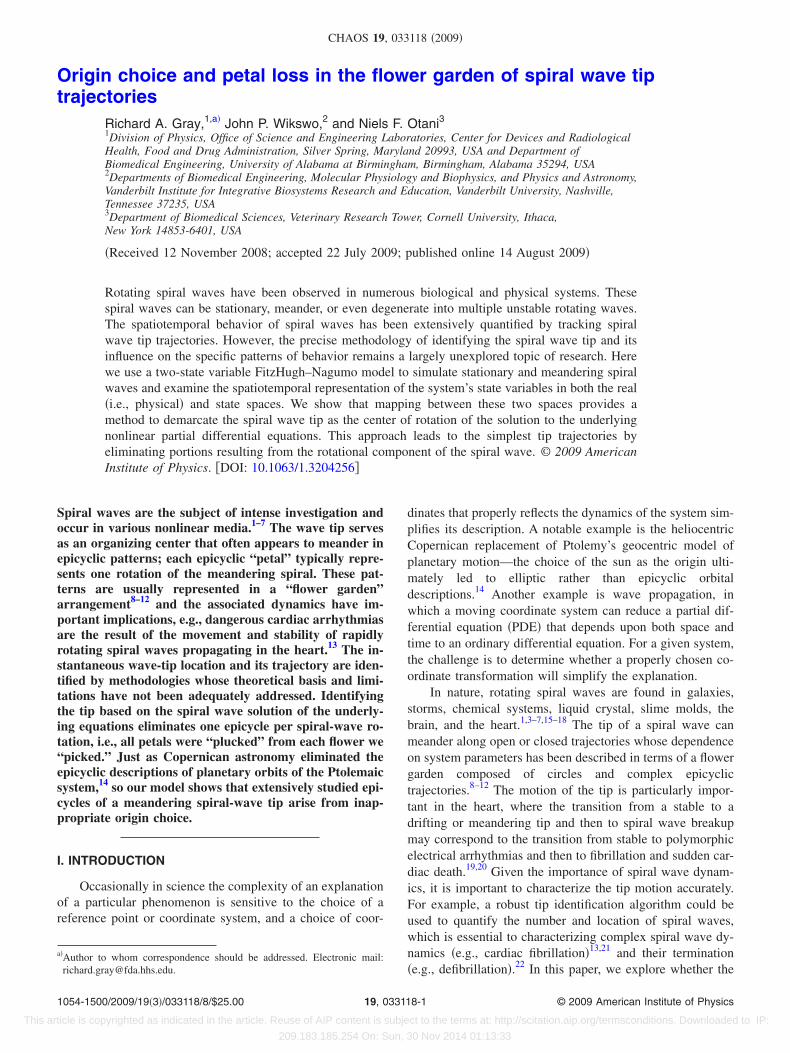
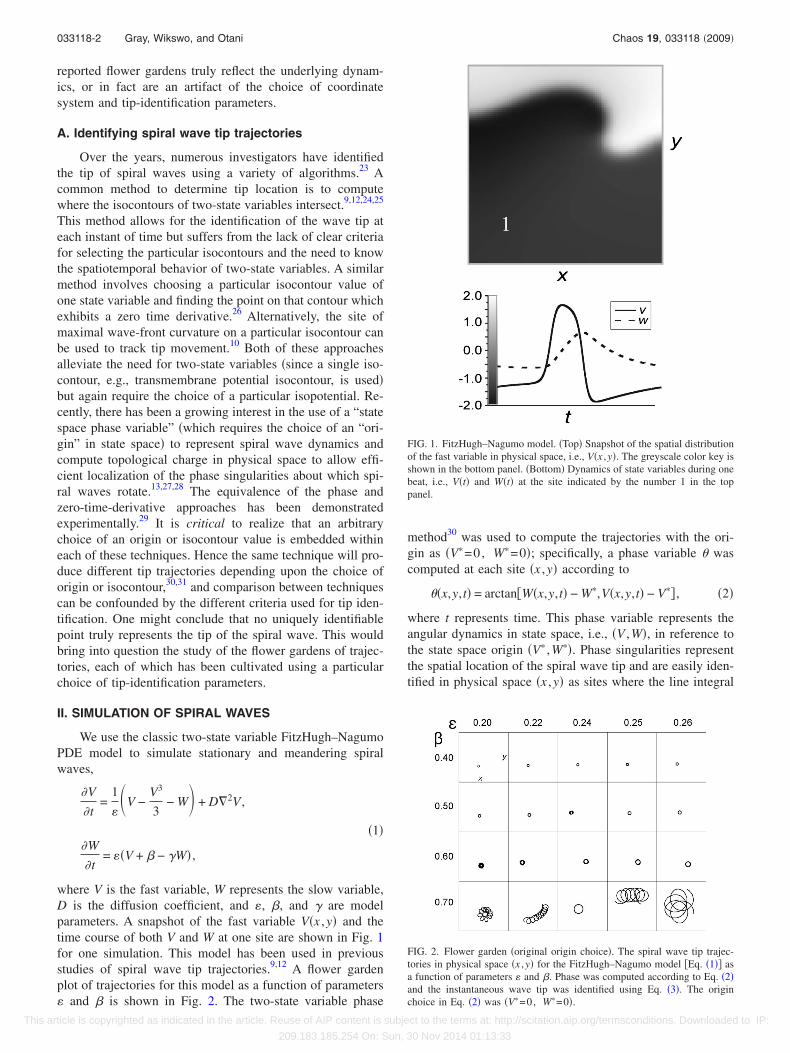
where V is the fast variable, W represents the slow variable,D is the diffusion coefficient, and �, �, and � are modelparameters. A snapshot of the fast variable V�x ,y� and thetime course of both V and W at one site are shown in Fig. 1for one simulation. This model has been used in previousstudies of spiral wave tip trajectories.9,12 A flower gardenplot of trajectories for this model as a function of parameters� and � is shown in Fig. 2. The two-state variable phase

method30 was used to compute the trajectories with the ori-gin as �V�=0, W�=0�; specifically, a phase variable � wascomputed at each site �x ,y� according to

��x,y,t� = arctan�W�x,y,t� − W�,V�x,y,t� − V�� , �2�

where t represents time. This phase variable represents theangular dynamics in state space, i.e., �V ,W�, in reference tothe state space origin �V� ,W��. Phase singularities representthe spatial location of the spiral wave tip and are easily iden-tified in physical space �x ,y� as sites where the line integral

FIG. 1. FitzHugh–Nagumo model. �Top� Snapshot of the spatial distributionof the fast variable in physical space, i.e., V�x ,y�. The greyscale color key isshown in the bottom panel. �Bottom� Dynamics of state variables during onebeat, i.e., V�t� and W�t� at the site indicated by the number 1 in the toppanel.

FIG. 2. Flower garden �original origin choice�. The spiral wave tip trajec-tories in physical space �x ,y� for the FitzHugh–Nagumo model �Eq. �1�� asa function of parameters � and �. Phase was computed according to Eq. �2�and the instantaneous wave tip was identified using Eq. �3�. The originchoice in Eq. �2� was �V�=0, W�=0�.

033118-2 Gray, Wikswo, and Otani Chaos 19, 033118 �2009�

This article is copyrighted as indicated in the article. Reuse of AIP content is subject to the terms at: http://scitation.aip.org/termsconditions. Downloaded to IP:

209.183.185.254 On: Sun, 30 Nov 2014 01:13:33

of � on a closed curve c around a site is nonzero, i.e.,

�c

�� · d�� � 0. �3�

Iyer and Gray30 showed that the ability to localize phasesingularities is not sensitively dependent on the specificchoice of state space origin �V� ,W��, and Fenton et al.31

showed examples of a minimal effect of isocontour choiceon tip trajectories. Nevertheless, to the best of our knowl-edge, there have been no published reports on the justifica-tion of a specific choice of origin. In addition, extending alltip finding methods to fibrillation data should only be donewith caution, and with a clear understanding of the algo-rithm’s limitations and theoretical basis. For example �as weshow below� inappropriate origin choice can lead to an errorin the identification of the number and lifetime of spiralwaves.

III. THEORY

Here we provide a rationale for choosing a specific statespace origin for the definition of � and hence phase singular-ity localization. Our goal here is essentially to track the in-stantaneous center of rotation of a spiral wave. In order to dothis, we need to separate the problem into two parts: spiralwave rotation around this center point and translational mo-tion of this center point. This problem is similar to the classiccharacterization of the rolling motion of a wheel on a planein which the trajectory of the center of mass follows astraight line but any other point traces out a nonlinear pathcalled a cycloid.

A rotating spiral wave represents one solution to the gen-eral nonlinear, reaction-diffusion PDE of the form

�u�

�t= f��u�� + D� �2u� , �4�

where u� is a vector representing the time and space depen-dent state variables, f� represents the nonlinear space-clampedkinetic equations for the variables, and D� is the diffusiontensor.

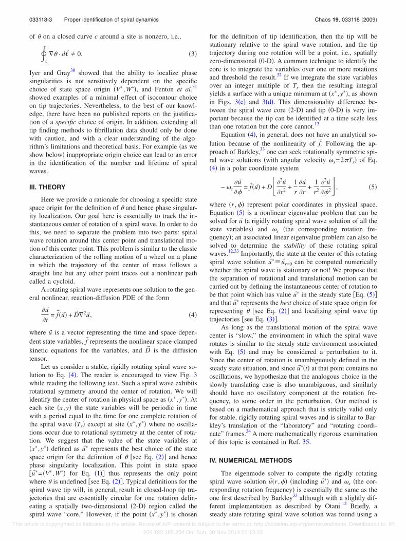
Let us consider a stable, rigidly rotating spiral wave so-lution to Eq. �4�. The reader is encouraged to view Fig. 3while reading the following text. Such a spiral wave exhibitsrotational symmetry around the center of rotation. We willidentify the center of rotation in physical space as �x� ,y��. Ateach site �x ,y� the state variables will be periodic in timewith a period equal to the time for one complete rotation ofthe spiral wave �Ts� except at site �x� ,y�� where no oscilla-tions occur due to rotational symmetry at the center of rota-tion. We suggest that the value of the state variables at�x� ,y�� defined as u�� represents the best choice of the statespace origin for the definition of � �see Eq. �2�� and hencephase singularity localization. This point in state space�u��= �V� ,W�� for Eq. �1�� thus represents the only pointwhere � is undefined �see Eq. �2��. Typical definitions for thespiral wave tip will, in general, result in closed-loop tip tra-jectories that are essentially circular for one rotation delin-eating a spatially two-dimensional �2-D� region called thespiral wave “core.” However, if the point �x� ,y�� is chosen

for the definition of tip identification, then the tip will bestationary relative to the spiral wave rotation, and the tiptrajectory during one rotation will be a point, i.e., spatiallyzero-dimensional �0-D�. A common technique to identify thecore is to integrate the variables over one or more rotationsand threshold the result.32 If we integrate the state variablesover an integer multiple of Ts then the resulting integralyields a surface with a unique minimum at �x� ,y��, as shownin Figs. 3�c� and 3�d�. This dimensionality difference be-tween the spiral wave core �2-D� and tip �0-D� is very im-portant because the tip can be identified at a time scale lessthan one rotation but the core cannot.13

Equation �4�, in general, does not have an analytical so-lution because of the nonlinearity of f�. Following the ap-proach of Barkley,33 one can seek rotationally symmetric spi-ral wave solutions �with angular velocity �s=2�Ts� of Eq.�4� in a polar coordinate system

− �s�u�

��= f��u�� + D� �2u�

�r2 +1

r

�u�

�r+

1

r2

�2u�

��2 , �5�

where �r ,�� represent polar coordinates in physical space.Equation �5� is a nonlinear eigenvalue problem that can besolved for u� �a rigidly rotating spiral wave solution of all thestate variables� and �s �the corresponding rotation fre-quency�; an associated linear eigenvalue problem can also besolved to determine the stability of these rotating spiralwaves.12,33 Importantly, the state at the center of this rotatingspiral wave solution u��u�r=0 can be computed numericallywhether the spiral wave is stationary or not! We propose thatthe separation of rotational and translational motion can becarried out by defining the instantaneous center of rotation tobe that point which has value u�� in the steady state �Eq. �5��and that u�� represents the best choice of state space origin forrepresenting � �see Eq. �2�� and localizing spiral wave tiptrajectories �see Eq. �3��.

As long as the translational motion of the spiral wavecenter is “slow,” the environment in which the spiral waverotates is similar to the steady state environment associatedwith Eq. �5� and may be considered a perturbation to it.Since the center of rotation is unambiguously defined in thesteady state situation, and since u���t� at that point contains nooscillations, we hypothesize that the analogous choice in theslowly translating case is also unambiguous, and similarlyshould have no oscillatory component at the rotation fre-quency, to some order in the perturbation. Our method isbased on a mathematical approach that is strictly valid onlyfor stable, rigidly rotating spiral waves and is similar to Bar-kley’s translation of the “laboratory” and “rotating coordi-nate” frames.34 A more mathematically rigorous examinationof this topic is contained in Ref. 35.

IV. NUMERICAL METHODS

The eigenmode solver to compute the rigidly rotatingspiral wave solution u��r ,�� �including u��� and �s �the cor-responding rotation frequency� is essentially the same as theone first described by Barkley33 although with a slightly dif-ferent implementation as described by Otani.12 Briefly, asteady state rotating spiral wave solution was found using a

033118-3 Proper identification of spiral dynamics Chaos 19, 033118 �2009�

This article is copyrighted as indicated in the article. Reuse of AIP content is subject to the terms at: http://scitation.aip.org/termsconditions. Downloaded to IP:

209.183.185.254 On: Sun, 30 Nov 2014 01:13:33

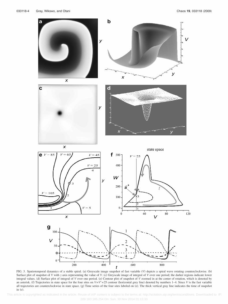
FIG. 3. Spatiotemporal dynamics of a stable spiral. �a� Greyscale image snapshot of fast variable �V� depicts a spiral wave rotating counterclockwise. �b�Surface plot of snapshot of V with z-axis representing the value of V. �c� Greyscale image of integral of V over one period; the darker regions indicate lowerintegral values. �d� Surface plot of integral of V over one period. �e� Contour plot of snapshot of V zoomed in at the center of rotation, which is denoted byan asterisk. �f� Trajectories in state space for the four sites on V=V�=25 contour �horizontal grey line� denoted by numbers 1–4. Since V is the fast variableall trajectories are counterclockwise in state space. �g� Time series of the four sites labeled on �e�. The thick vertical gray line indicates the time of snapshotin �e�.

033118-4 Gray, Wikswo, and Otani Chaos 19, 033118 �2009�

This article is copyrighted as indicated in the article. Reuse of AIP content is subject to the terms at: http://scitation.aip.org/termsconditions. Downloaded to IP:

209.183.185.254 On: Sun, 30 Nov 2014 01:13:33

nonlinear eigenmode solver in polar coordinates given initialguesses of both the spiral wave frequency and a spatial pat-tern of u� . We determined u�� for the PDE in Eq. �1� for 20parameter values ��=0.20,0.22,0.24,0.25,0.26 and �=0.40,0.50,0.60,0.70� using the methodology describedpreviously.12,33 These values are presented in Table I for ourtwo-variable system u��= �V� ,W��.

We simulated stationary and nonstationary spiral wavesby integrating Eq. �1� using finite difference methods on auniform x-y grid. We used the values of D=0.003 and �=0.8and varied both � and �. This PDE was solved on a500�500 grid with no-flux boundary conditions via Eulerintegration with grid spacing dx=dy=0.04 and time stepdt=0.0004.

V. RESULTS

The effect of the origin choice on spiral wave tip trajec-tories is shown for �=0.22 and �=0.70 in Fig. 4. The vari-able represents the distance of the origin choice from u��; tostudy the effect of the choice of the origin, was chosen tovary along the diagonal line V=W �see Fig. 4�d��. The spiralwave tip trajectory was a strong function of ; as increasedfrom zero, one loop was formed per rotation and these loopsincreased in size. In other words, one petal per rotation ap-peared on the tip trajectory for “incorrect” choices of statespace origin ��0�. The flower garden in Fig. 2 was repro-duced using u�� as the origin choice and is shown in Fig. 5.For all parameter choices of � and �, the choice of u�� as theorigin for the computation of phase ��� in Eq. �2� resulted ina decrease in complexity of the spiral wave tip trajectories�compare Figs. 5 and 2�. Circular trajectories became pointsand looping patterns became lines.

The value of u�� depends on the parameter values of thePDE. That is, changes in � and � alter the solution to Eq. �5�and hence u�� at the center of rotation. The position of u�� instate space is shown for each parameter set in Fig. 6; u�� isrepresented as an asterisk and the elliptical curves representtypical dynamics at one site of variables V and W in statespace �V ,W�.

VI. DISCUSSION

The advantage of using u�� in defining state space phase��� in Eq. �2� is that it maps to the exact center of rotation forthe case that is arguably the best representative and mostcharacteristic of pure spiral wave rotation for the given sys-tem, namely, rigid spiral wave rotation around a fixed point.Thus, the point at which u��=u� is a natural candidate for the

definition of the spiral wave tip location—a Copernicanchoice in an otherwise Ptolemeic situation. Our rationale isconsistent with the idea that spiral wave meandering is aperturbation of the steady state solution to Eq. �5�.33

The spiral wave tip trajectories for the traditional choiceof origin �V=0 and W=0� are not the simplest, as shown inFig. 2. The value of the origin that produces the simplestpattern corresponds to u��, as shown in Fig. 5, which in turndepends on the parameter values of the PDE. That is,changes in parameters that produce the observed varieties inthe garden also shift the solution to Eq. �5� at the center of

TABLE I. The values of the solution to Eq. �5� at the center of rotation, i.e., u��= �V� ,W�� for the FitzHugh–Nagumo equation �Eq. �1��, as a function of the two model parameters � and �.

�

�

0.20 0.22 0.24 0.25 0.26

0.40 �0.637,0.296� �0.644,0.304� �0.651,0.313� �0.654,0.318� �0.658,0.323�0.50 �0.796,0.370� �0.806,0.382� �0.817,0.396� �0.823,0.403� �0.829,0.411�0.60 �0.955,0.444� �0.970,0.463� �0.988,0.486� �1.00,0.500� �1.01,0.516�0.70 �1.11,0.517� �1.14,0.548� �1.18,0.604� �1.20,0.623� �1.20,0.624�

FIG. 4. The spiral wave tip trajectories in the FitzHugh–Nagumo model�Eq. �1�; �=0.22 and �=0.70� as a function of origin choice. �a� Phase wascomputed according to Eq. �2� and the instantaneous wave tip was identifiedusing Eq. �3�. The height of the plot, i.e., the vertical axis, represents thedistance from u�� defined as =��V−V��2+ �W−W��2. �b� Spiral tip trajec-tory for =0.75. �c� Spiral tip trajectory for =0.0. �d� Schematic diagramillustrating choice of along the diagonal in state space.

033118-5 Proper identification of spiral dynamics Chaos 19, 033118 �2009�

This article is copyrighted as indicated in the article. Reuse of AIP content is subject to the terms at: http://scitation.aip.org/termsconditions. Downloaded to IP:

209.183.185.254 On: Sun, 30 Nov 2014 01:13:33

rotation, as shown in Fig. 6. Our results demonstrate that ifthe origin is adjusted in accordance with the parameter shiftfor each plant in the garden, so as to maintain the correspon-dence between the solution to Eq. �5� at the center of rotationand the origin, then the garden reduces to a simpler set ofcurves. We suggest that the origin choice of u�� is the best inthe sense that it separates the rotational and translational mo-tions of the spiral wave. One may argue that the flower petalsillustrate each spiral wave rotation, and while this can betrue, it is not necessarily true. We can see no reason why thespiral wave cannot complete multiple rotations during thetime it takes for the trajectory to trace out one completepetal. Since time is parametrized in the tip trajectory plots, ingeneral, we do not know the speed of movement along thetrajectory nor Ts just from viewing the tip trajectories �al-

though the speed can easily be computed�. In our approachwe compute Ts via � and u�� and the corresponding trajecto-ries represent only translational movement.

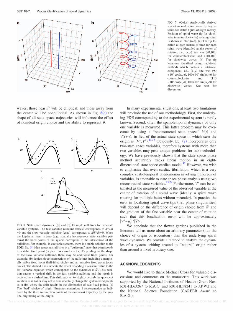
Not using the center of rotation to identify spiral wavetip dynamics can give rise to errors in the identification ofthe number and lifetime of spiral waves when multiplewaves are present, as shown in Fig. 7. An episode of fibril-lation as recorded from the heart surface can be representedby the number, location, and chirality of spiral waves at eachinstant in time.13 We illustrate the tip trajectories of a hypo-thetical stable figure-of-eight pair of spiral waves in Fig. 7�in panel �a�, the tip is identified as the center of rotation andthus the location of each spiral wave is stationary, while inpanel �b�, the tip is identified using traditional methods andeach trajectory exhibits a cycloid pattern�. Since the identi-fication of phase singularities �see Eq. �3�� involves a spatialline integral, the exact line integral determines the lowerlimit �spatial resolution� on the localization of spiral wavetips. For example, if at a given instant both spiral wave tipsare within the line integral of Eq. �3�, then no phase singu-larities will be detected instead of two �one clockwise andone counterclockwise�! This will result in the erroneous in-ference that there is continuous birth and termination of twocounter-rotating spiral waves instead of a continuous pair ofstable counter-rotating spiral waves. Using the center of ro-tation to identify spiral wave tips will result in the correctinterpretation.

The state space representation of phase ��� depends onthe choice of origin as previously stated. It should be appre-ciated that u�� is, in general, not equal to a fixed point in thespace-clamped 0-D situation because the Laplacian term inEq. �1� is nonzero. In fact, u�� can be much different than thesteady state homogenous solution because of the topology ofstate space, as shown in Figs. 8�a� and 8�b�. Trajectories instate space will always be closed curves for stable spiral

FIG. 5. Flower garden �origin=u���. The spiral wave tip trajectories in physi-cal space �x ,y� for the FitzHugh–Nagumo model �Eq. �1�� as a function ofparameters � and �. Phase was computed according to Eq. �2� and theinstantaneous wave tip was identified using Eq. �3�. The origin choice in Eq.�2� was u�� in contrast to �0,0� in Fig. 2 for the same parameter values of �and �.

FIG. 6. The dynamics of state variables �V and W� in state space for one site during spiral wave rotation as a function of � and �. The locations of u�� �seeTable I� are shown as asterisks. For clarity, the axis labels are only shown in the top left plot. The origin �0,0� axes are indicated by dashed lines.

033118-6 Gray, Wikswo, and Otani Chaos 19, 033118 �2009�

This article is copyrighted as indicated in the article. Reuse of AIP content is subject to the terms at: http://scitation.aip.org/termsconditions. Downloaded to IP:

209.183.185.254 On: Sun, 30 Nov 2014 01:13:33

waves; those near u�� will be elliptical, and those away fromthe center will be nonelliptical. As shown in Fig. 8�c� theshape of all state space trajectories will influence the effectof nonideal origin choice and the ability to represent �.

In many experimental situations, at least two limitationswill preclude the use of our methodology. First, the underly-ing PDE corresponding to the experimental system is rarelyknown. Second, often the spatiotemporal dynamics of onlyone variable is measured. This latter problem may be over-come by using a “reconstructed state space,” V�t� andV�t+��, in lieu of the actual state space in which case theorigin is �V� ,V��.13,36 Obviously, Eq. �2� incorporates onlytwo-state space variables, therefore systems with more thantwo variables may pose unique problems for our methodol-ogy. We have previously shown that the state space phasemethod accurately tracks linear motion in an eight-dimensional state space cardiac model.37 However, we wishto emphasize that even cardiac fibrillation, which is a verycomplex spatiotemporal phenomenon involving hundreds ofvariables, is amenable to state space phase analysis using tworeconstructed state variables.13,22 Furthermore, V� can be es-timated as the measured value of the observed variable at thecenter of rotation of a spiral wave �ideally, a spiral waverotating for multiple beats without meander�. In practice theerror in localizing spiral wave tips �i.e., phase singularities�will depend on the difference of origin choice from u�� andthe gradient of the fast variable near the center of rotationsuch that this localization error will be approximately�V�−u1

�� / ��V�.We conclude that the flower gardens published in the

literature tell us more about an arbitrary parameter �i.e., thechoice of origin or isocontour� than the underlying spiralwave dynamics. We provide a method to analyze the dynam-ics of a system orbiting around its “natural” origin ratherthan around a fixed arbitrary one.

ACKNOWLEDGMENTS

We would like to thank Michael Cross for valuable dis-cussions and comments on the manuscript. This work wassupported by the National Institutes of Health �Grant Nos.R01-HL63267 to R.A.G. and R01-HL58241 to J.P.W.� andthe National Science Foundation �CAREER Award toR.A.G.�.

FIG. 7. �Color� Analytically derivedspatiotemporal spiral wave tip trajec-tories for stable figure-of-eight reentry.Position of spiral wave tip for clock-wise �counterclockwise� rotating spiralis shown in blue �red�. �a� The tip lo-cation at each instant of time for eachspiral wave identified as the center ofrotation, i.e., �x ,y� site was �90,100�for counterclockwise and �110,100�for clockwise waves. �b� The tiplocations identified using traditionalmethods which contain a rotationalcomponent, i.e., �x ,y� site was �90+10� cos��s�t�, 100+10� sin��s�t�� forcounterclockwise and �110−10� cos��s�t�, 100+10� sin��s�t�� forclockwise waves. See text fordiscussion.

FIG. 8. State space dynamics. ��a� and �b�� Example nullclines for two-statevariable systems. The fast variable nullcline �black� corresponds to dV /dt=0 and the slow variable nullcline �gray� corresponds to dW /dt=0. Whenthe Laplacian term is zero �e.g., spatially homogenous state variable pat-terns� the fixed points of the system correspond to the intersection of thenullclines. For example, in excitable systems, there is a stable solution to thePDE �Eq. �4�� that represents all sites at a “quiescent” state that correspondsto a stable fixed point �depicted as closed circles�. Depending on the shapeof the slow variable nullcline, there may be additional fixed points. Forexample, �b� depicts three intersections of the nullclines including a margin-ally stable fixed point �half-filled circle� and an unstable fixed point �opencircle�. The dashed lines indicate the effect of adding a constant value to thefast variable equation which corresponds to the dynamics at u��. This addi-tion causes a vertical shift in the fast variable nullcline and the result isdepicted as a dashed line. This shift may act to slightly perturb the quiescentsolution as in �a� or may act to fundamentally change the system fixed pointsas in �b�, where the shift results in the elimination of two fixed points. �c�The “bad” choice of origin illustrates nonunique � representation as indi-cated by the three intersection points of the outermost trajectory by the grayline originating at the origin.

033118-7 Proper identification of spiral dynamics Chaos 19, 033118 �2009�

This article is copyrighted as indicated in the article. Reuse of AIP content is subject to the terms at: http://scitation.aip.org/termsconditions. Downloaded to IP:

209.183.185.254 On: Sun, 30 Nov 2014 01:13:33

1A. Goldbeter, Nature �London� 253, 540 �1975�.2A. T. Winfree, The Geometry of Biological Time �Springer-Verlag, Berlin,1980�, Vol. XIII, p. 530.

3J. Lechleiter, S. Girard, E. Peralta, and D. Clapham, Science 252, 123�1991�.

4O. Steinbock, V. Zykov, and S. C. Muller, Nature �London� 366, 322�1993�.

5G. Li, Q. Ouyang, V. Petrov, and H. L. Swinney, Phys. Rev. Lett. 77,2105 �1996�.

6M. Vinson, S. Mironov, S. Mulvey, and A. Pertsov, Nature �London� 386,477 �1997�.

7M. Bazhenov, I. Timofeev, M. Steriade, and T. J. Sejnowski, Nat. Neuro-sci. 2, 168 �1999�.

8V. S. Zykov, Biofizika 25, 906 �1986�.9A. T. Winfree, Chaos 1, 303 �1991�.

10J. Beaumont, N. Davidenko, J. Davidenko, and J. Jalife, Biophys. J. 75, 1�1998�.

11Z. Qu, J. N. Weiss, and A. Garfinkel, Am. J. Physiol. 276, H269 �1999�.12N. F. Otani, Chaos 12, 829 �2002�.13R. A. Gray, A. M. Pertsov, and J. Jalife, Nature �London� 392, 75 �1998�.14N. Copernicus, De Revolutionibus Orbium Caelestium, edited by T. B. A.

M. Duncan �Newton Abbot, New York, 1976�, p. 1543.15A. T. Winfree, When Time Breaks Down: The Three-Dimensional Dynam-

ics of Electrochemical Waves and Cardiac Arrhythmias �Princeton Univer-sity Press, Princeton, NJ, 1987�, Vol. XIV, p. 339.

16X. Huang, W. C. Troy, Q. Yang, H. Ma, C. R. Laing, S. J. Schiff, and J.-Y.Wu, J. Neurosci. 24, 9897 �2004�.

17R. H. Clayton and A. V. Holden, IEEE Trans. Biomed. Eng. 51, 28�2004�.

18A. V. Panfilov, Heart Rhythm 3, 862 �2006�.19R. A. Gray, J. Jalife, A. V. Panfilov, W. T. Baxter, C. Cabo, J. M. Dav-

idenko, A. M. Pertsov, Science 270, 1222 �1995�.

20R. A. Gray, J. Jalife, A. Panfilov, W. T. Baxter, C. Cabo, J. M. Davidenko,and A. M. Pertsov, Circulation 91, 2454 �1995�.

21M. A. Bray and J. P. Wikswo, Phys. Rev. Lett. 90, 238303 �2003�.22R. A. Gray and N. Chattipakorn, Proc. Natl. Acad. Sci. U.S.A. 102, 4672

�2005�.23R. H. Clayton, E. A. Zhuchkova, and A. V. Panfilov, Prog. Biophys. Mol.

Biol. 90, 378 �2006�.24V. G. Fast and A. M. Pertsov, Biofizika 35, 478 �1990�.25F. Fenton and A. Karma, Chaos 8, 20 �1998�.26R. Mandapati et al., Circulation 98, 1688 �1998�.27M. A. Bray, S.-F. Lin, R. R. Aliev, B. J. Roth, and J. P. Wikswo, Jr., J.

Cardiovasc. Electrophysiol. 12, 716 �2001�.28S. Puwal, B. J. Roth, and S. Kruk, IMA J. Math. Appl. Med. Biol. 22, 335

�2005�.29Y. B. Liu, A. Peter, S. T. Lamp, J. N. Weiss, P.-S. Chen, and S.-F. Lin, J.

Cardiovasc. Electrophysiol. 14, 1103 �2003�.30A. N. Iyer and R. A. Gray, Ann. Biomed. Eng. 29, 47 �2001�.31F. H. Fenton, E. M. Cherry, H. M. Hastings, and S. J. Evans, Chaos 12,

852 �2002�.32J. M. Davidenko, A. V. Pertsov, R. Salomonsz, W. Baxter, and J. Jalife,

Nature �London� 355, 349 �1992�.33D. Barkley, Phys. Rev. Lett. 68, 2090 �1992�.34D. Barkley, M. Kness, and L. S. Tuckerman, Phys. Rev. A 42, 2489

�1990�.35V. N. Biktashev and A. V. Holden, Proc. R. Soc. London, Ser. B 263,

1373 �1996�.36F. Takens, in Dynamical Systems and Turbulence, edited by D. A. Rand

and L. S. Young �Springer-Verlag, Berlin, 1981�, pp. 366–381.37A. Iyer and R. A. Gray, Pacing Clin. Electrophysiol. 24, 692 �2001�.

033118-8 Gray, Wikswo, and Otani Chaos 19, 033118 �2009�

This article is copyrighted as indicated in the article. Reuse of AIP content is subject to the terms at: http://scitation.aip.org/termsconditions. Downloaded to IP:

209.183.185.254 On: Sun, 30 Nov 2014 01:13:33