optimizing membrane distillation process for triethylene...
TRANSCRIPT
i
Optimizing Membrane Distillation Process for Triethylene Glycol
Separation from Gas Separation Plant Waste Stream
by
Pham Minh Duyen
A thesis submitted in partial fulfillment of the requirements for the
degree of Master of Engineering in
Environmental Engineering and Management
Examination Committee: Prof. Chettiyappan Visvanathan (Chairperson)
Dr. Thammarat Koottatep
Dr. Romchat Rattanaoudom (External Expert)
Nationality: Vietnamese
Previous Degree: Bachelor of Engineering in Environmental Engineering
Ho Chi Minh City University of Technology
Vietnam
Scholarship Donor: Greater Mekong Subregion (GMS) Scholarship
Asian Institute of Technology
School of Environment, Resources and Development
Thailand
May 2015

ii
Acknowledgments
My master thesis would not have been possible to achieve without the support of many
kind people. It is my pleasure to acknowledge everyone who has supported me to achieve
this thesis and also my master degree.
Above all, I would like to express my heartfelt gratitude to my advisor, Prof. C.
Visvanathan. This thesis would never have been achieved without his encouragement and
kind patience along this challenging journey. I am truly thankful for his helpful advice and
technical suggestions. By having Prof. C. Visvanathan as advisor, I have improved the
confidence in both academic and personal sides.
I also would like to show my appreciation to my thesis’s committee members, Dr.
Thammarat Koottatep and Dr. Romchat Rattannaoudom. Their useful advice, support and
encouragement have been invaluable upon the completion of my thesis.
I am sincerely thankful to EEM faculties and staffs. Mr. Panupong and Mr. Nimitra are two
technicians of EEM who I am most grateful to. The experimental set-up would not be
controlled, fixed and improved without their technical support. I wish to deliver my grateful
appreciation to Mr. Chaiyaporn who provided laboratory facilities and analysis information
together with many important advice. Furthermore, I want to thank Ms. Suchitra, Ms.
Chanya, Ms. Salaya amd Ms. Orathai for their kind support and encouragement. Especially,
I am grateful to Ms. Suchitra who always took care of me in both academic and personal
life, and encouraged me to move on.
My special thanks also go to Prof. C. Visvanathan’s research group. I am happy to have
worked alongside this highly motivated team during my master thesis. Mr. Thusitha and
Mr. Jacob acted as helpful mentors with many critical technical input for my study.
For my colleagues, Kung, My, Thi, Aashik, Ju Ju, Milk and Mr. Park, thank you all for
your help and support. It is very appreciated to your sharing important information and
suggestion, especially our great friendship.
I thankfully acknowledge and appreciate the Royal Thai Government for the financial
support with Loom Nam Khong Pijai (GMSARN) scholarship in order for me to pursue
the master program. My sincere thanks are expressed to PTT Public Company Limited
(Thailand) for providing wastewater and conducting wastewater analysis throughout this
research. Especially, my appreciation is expressed for the AIT-PTT-II project for the
research grant.
Last but not least, to my dear family, all my expression of gratitude does not suffice. I am
grateful for their love, encouragement and support. I want to say thank you for their
understanding and being my home no matter what I did, especially during my away-from-
home mission.
iii
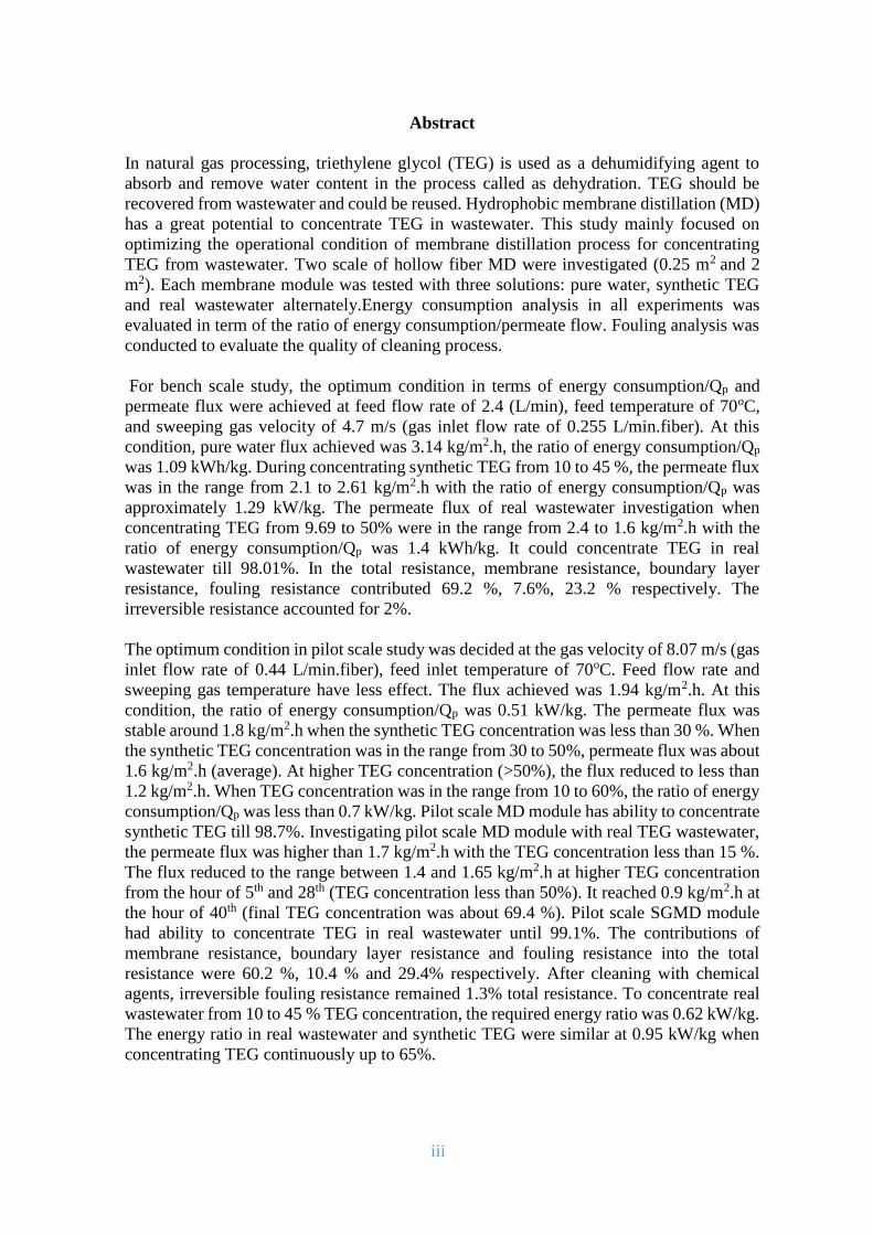
Abstract
In natural gas processing, triethylene glycol (TEG) is used as a dehumidifying agent to
absorb and remove water content in the process called as dehydration. TEG should be
recovered from wastewater and could be reused. Hydrophobic membrane distillation (MD)
has a great potential to concentrate TEG in wastewater. This study mainly focused on
optimizing the operational condition of membrane distillation process for concentrating
TEG from wastewater. Two scale of hollow fiber MD were investigated (0.25 m2 and 2
m2). Each membrane module was tested with three solutions: pure water, synthetic TEG
and real wastewater alternately.Energy consumption analysis in all experiments was
evaluated in term of the ratio of energy consumption/permeate flow. Fouling analysis was
conducted to evaluate the quality of cleaning process.
For bench scale study, the optimum condition in terms of energy consumption/Qp and
permeate flux were achieved at feed flow rate of 2.4 (L/min), feed temperature of 70oC,
and sweeping gas velocity of 4.7 m/s (gas inlet flow rate of 0.255 L/min.fiber). At this
condition, pure water flux achieved was 3.14 kg/m2.h, the ratio of energy consumption/Qp
was 1.09 kWh/kg. During concentrating synthetic TEG from 10 to 45 %, the permeate flux
was in the range from 2.1 to 2.61 kg/m2.h with the ratio of energy consumption/Qp was
approximately 1.29 kW/kg. The permeate flux of real wastewater investigation when
concentrating TEG from 9.69 to 50% were in the range from 2.4 to 1.6 kg/m2.h with the
ratio of energy consumption/Qp was 1.4 kWh/kg. It could concentrate TEG in real
wastewater till 98.01%. In the total resistance, membrane resistance, boundary layer
resistance, fouling resistance contributed 69.2 %, 7.6%, 23.2 % respectively. The
irreversible resistance accounted for 2%.
The optimum condition in pilot scale study was decided at the gas velocity of 8.07 m/s (gas
inlet flow rate of 0.44 L/min.fiber), feed inlet temperature of 70oC. Feed flow rate and
sweeping gas temperature have less effect. The flux achieved was 1.94 kg/m2.h. At this
condition, the ratio of energy consumption/Qp was 0.51 kW/kg. The permeate flux was
stable around 1.8 kg/m2.h when the synthetic TEG concentration was less than 30 %. When
the synthetic TEG concentration was in the range from 30 to 50%, permeate flux was about
1.6 kg/m2.h (average). At higher TEG concentration (>50%), the flux reduced to less than
1.2 kg/m2.h. When TEG concentration was in the range from 10 to 60%, the ratio of energy
consumption/Qp was less than 0.7 kW/kg. Pilot scale MD module has ability to concentrate
synthetic TEG till 98.7%. Investigating pilot scale MD module with real TEG wastewater,
the permeate flux was higher than 1.7 kg/m2.h with the TEG concentration less than 15 %.
The flux reduced to the range between 1.4 and 1.65 kg/m2.h at higher TEG concentration
from the hour of 5th and 28th (TEG concentration less than 50%). It reached 0.9 kg/m2.h at
the hour of 40th (final TEG concentration was about 69.4 %). Pilot scale SGMD module
had ability to concentrate TEG in real wastewater until 99.1%. The contributions of
membrane resistance, boundary layer resistance and fouling resistance into the total
resistance were 60.2 %, 10.4 % and 29.4% respectively. After cleaning with chemical
agents, irreversible fouling resistance remained 1.3% total resistance. To concentrate real
wastewater from 10 to 45 % TEG concentration, the required energy ratio was 0.62 kW/kg.
The energy ratio in real wastewater and synthetic TEG were similar at 0.95 kW/kg when
concentrating TEG continuously up to 65%.

iv
Graphical Abstract
1
Table of Contents
Chapter Title Page
Title Page
Acknowledgements
Abstract
Graphical Abstract
Table of Contents
List of Tables
List of Figures
List of Abbreviations
i
ii
iii
iv
v
ix
xi
xiv
1
2
3
4
Introduction
1.1 Background
1.2 Objectives of the Study
1.3 Scope of the Study
Literature Review
2.1 Natural Gas Industry Overview
2.2 Triethylene Glycol
2.3 Membrane Science and Technology
2.4 Membrane Distillation
2.5 Material of Membrane and Module Fabrications Using for
Distillation Process
2.6. Operational Processes of Membrane Distillation
2.7 Temperature Polarization
2.8 Concentration Polarization
2.9 Membrane Fouling
2.10 Membrane Cleaning
2.11 Operating Variables Affecting MD Process
2.12 Effects of Membrane Parameters on MD Process
2.13Advantages and Limitations of Membrane Distillation
Technology
2.14 Application of Membrane Distillation
2.15 Research Gap
Methodology
3.1 Methodology Overview
3.2 Experimental Materials
3.3 Experimental Methods
3.4 Experimental Analysis
Results and Discussions
4.1 TEG Wastewater Characterization
4.2 Performance of Pre-treatment Unit
4.3 Optimizing Operation of Bench Scale Hollow Fiber SGMD
4.4 optimum condition of pilot scale SGMD and evaluate energy
4.5 Full Scale SGMD Plant Design
1
2
2
2
3
8
12
13
17
18
25
26
27
29
29
33
35
36
37
39
39
41
44
51
54
54
55
56
79
104

2
5
Conclusions and Recommendations
5.1 Conclusions
5.2 Recommendations for Future Study
Reference
Appendix A
Appendix B
Appendix C
Appendix D
Appendix E
Appendix F
108
108
110
112
118
123
151
163
174
200
3
List of Tables
Table
Title Page
2.1 Components of Natural Gas 3
2.2 Properties of Natural Gas 4
2.3 Properties of Triethylene Glycol 9
2.4 TEG Applications 10
2.5 General Characteristics of Membrane Process 16
2.6 Effect of Variables on Permeate Flux in MD Process 32
2.7 Effect of Membrane Parameter on Permeate Flux in MD Process 32
2.8 Typical Fields of MD Application 37
2.9 Overview of Various TEG Separation Processes 37
3.1 MF and UF Membrane Properties in Pre-treatment Unit 41
3.2 Hollow Fiber Membrane Distillation Specification 42
3.3 Membrane Distillation Module Specification 43
3.4 Cleaning Chemicals Used in this Study 44
3.5 Membrane Cleaning Procedure 51
3.6 Analytical Parameters and Methods 53
4.1 Wastewater Analytical Results 54
4.2 Analytical Results of Pre-treating Samples 55
4.3 The Ratio of Energy Consumption/Qp at Different Scenarios of Pure
Water Test
61
4.4 PWF Comparison with Other Studies on SGMD 63
4.5 Membrane Surface Temperature and Temperature Polarization
Coefficient
64
4.6
Experimental Membrane Distillation Coefficient and Membrane
Resistance
64
4.7 TEG Concentration in Synthetic TEG Test 65
4.8 Membrane Resistance and Boundary Layer Resistance 68
4.9 Total Membrane Boundary Layer and Fouling Resistance Calculated
from Fouled Permeate Flux (batch operation)
72
4.10 Total Membrane Boundary Layer and Fouling Resistance Calculated
from Fouled Permeate Flux (continuously-fed operation)
73
4.11 Comparison of Fouling and Other Resistance between Continuously-fed
and Batch Operation
74
4.12 Comparison of Fouling and Other Resistance between SGMD and
DCMD Bench Scale Hollow Fiber Membrane Distillation
(Continuously-fed)
75
4.13 Experimental Results of PWF Investigation on Pilot Scale Module 81
4.14 Membrane Resistance and Membrane Coefficient 81
4.15 Membrane Resistance and Boundary Layer Resistance 89
4.16 Total Membrane Boundary Layer and Fouling Resistance Calculated
from Fouled Permeate Flux
92
4.17 Total Membrane Boundary Layer and Fouling Resistance Calculated
from Fouled Permeate Flux (continuously-fed operation)
94
4.18 Comparison of Fouling and Other Resistance between Continuously-fed
and Batch Operation
95
4
4.19 Comparison of Fouling and Other Resistance between Normal
Condition and 0ptimum Condition of SGMD Hollow Fiber Membrane
Distillation (Continuously-fed)
96
4.20 Summary of Financial Analysis for Overall System with ±30% Variation 107

5
List of Figures
Figure
Title Page
2.1 Natural gas use by sector 5
2.2 Products of gas separation plant and applications 6
2.3 Natural gas processing 7
2.4 Triethylene glycol wastewater steam of PTT’s gas separation plant 8
2.5 Break down of TEG application in US 9
2.6 Vapor-liquid interface in membrane distillation 14
2.7 Four configurations of membrane distillation process 14
2.8 Dusty gas model 21
2.9 Poiseuille type of flow inside a pore of SGMD process 23
2.10 Temperature and concentration profile in MD process 26
2.11 Concentration and temperature polarization in MD process 27
2.12 Profile of temperature in fouling case 28
3.1 Experimental study plan 40
3.2 Experimental materials using in this research 41
3.3 Schematic diagram of pre-treatment unit 45
3.4 Image of pre-treatment system 45
3.5 Cross flow mode description in sweep gas membrane distillation 46
3.6 Bench scale hollow fiber sweep gas membrane distillation 46
3.7 Image of bench scale hollow fiber SGMD system 46
3.8 Pilot scale hollow fiber sweep gas membrane distillation unit 47
3.9 The principle of sweeping gas membrane distillation configuration 48
3.10 Determination process of fouling resistances 52
4.1 Removal efficiency of pre-treatment system 56
4.2 Rejection result of hollow fiber SGMD at gas velocity of 3.1 m/s 57
4.3 Rejection result of hollow fiber SGMD at gas velocity of 5.3 m/s 58
4.4 Permeate flux at different feed inlet flow rate and sweeping gas velocity at
feed temperature of 70oC
59
4.5 Permeate flux at different feed inlet temperature and sweeping gas velocity at
feed flow rate of 2.4 L/min
59
4.6 Energy consumption/Qp at feed flow rate of 2.4 L/min 61
4.7 Permeate flux and TEG concentration at synthetic TEG 10% initial
concentration
65
4.8 Permeate flux and TEG concentration at synthetic TEG 30% initial
concentration
66
4.9 Permeate flux and TEG concentration at synthetic TEG 60% initial
concentration
67
4.10 Experimental result of continuously-fed synthetic TEG investigation 67
4.11 Increasing of boundary layer resistance 69
4.12 Experimental results of batch experiment with real wastewater. 70
4.13 Experimental result of continuously-fed real wastewater investigation 71
4.14 Permeate flux and TEG concentration during 210 hrs feeding continuously 71
4.15 Classification of types of resistances in SGMD batch operation 73
4.16 Resistance classification in SGMD continuously-fed real wastewater 74
6
4.17 Energy Consumption/Qp during concentrating TEG at 10% initial
concentration
76
4.18 Energy Consumption/Qp during concentrating TEG at 30% initial
concentration
76
4.19 Energy Consumption/Qp during concentrating TEG at 60% initial
concentration
77
4.20 Energy Consumption/Qp during concentrating TEG for 40 hours 77
4.21 Energy Consumption/Qp of batch experiment with real wastewater. 78
4.22 Energy Consumption/Qp of continuously-fed experiments with real
wastewater.
79
4.23 Pure water flux at different sweeping gas inlet flow rate of pilot scale study 80
4.24 Rejection results for pilot scale SGMD process of pilot scale study 82
4.25 Permeate flux and TEG concentration synthetic TEG 10% initial
concentration of pilot scale study
83
4.26 Permeate flux and TEG concentration synthetic TEG 25% initial
concentration of pilot scale study
83
4.27 Permeate flux and TEG concentration synthetic TEG 40% initial
concentration of pilot scale study
84
4.28 Permeate flux and TEG concentration synthetic TEG 60% initial concentration
of pilot scale study
84
4.29 Permeate flux and TEG concentration synthetic TEG 80% initial
concentration of pilot scale study
85
4.30 Permeate flux and TEG concentration at synthetic TEG 10% initial
concentration of pilot scale study
85
4.31 Permeate flux and TEG concentration at synthetic TEG 20% initial
concentration of pilot scale study
86
4.32 Permeate flux and TEG concentration at synthetic TEG 30% initial
concentration of pilot scale study
87
4.33 Permeate flux and TEG concentration at synthetic TEG 40% initial
concentration of pilot scale study
87
4.34 Permeate flux and TEG concentration at synthetic TEG 60% initial
concentration of pilot scale study
88
4.35 Experimental result of continuously-fed synthetic TEG investigation of pilot
scale study
89
4.36 Proportion of Boundary Layer Resistance and Membrane Resistance of pilot
scale study
90
4.37 Experimental results of batch experiment with real wastewater of pilot scale
study
91
4.38 Classification of types of resistances in SGMD batch operation of pilot scale
study
92
4.39 Experimental result of continuously-fed real wastewater investigation of pilot
scale study (40 hours)
93
4.40 Experimental result of continuously-fed real wastewater investigation of pilot
scale study (72 hours)
94
4.41 Classification of resistances in SGMD continuously-fed real wastewater of
pilot scale study
95
4.42 Inlet velocity distribution in hollow fiber module 97
4.43 Local velocities inside membrane module 98
7
4.44 Energy Consumption/Qp during concentrating TEG at 10% initial
concentration of pilot scale study
99
4.45 Energy Consumption/Qp during concentrating TEG at 20% initial
concentration of pilot scale study
99
4.46 Energy Consumption/Qp during concentrating TEG at 30% initial
concentration of pilot scale study
100
4.47 Energy Consumption/Qp during concentrating TEG at 40% initial
concentration of pilot scale study
100
4.48 Energy Consumption/Qp during concentrating TEG at 60% initial
concentration of pilot scale study
101
4.49 Energy Consumption/Qp during concentrating TEG for 40 hours of pilot scale
study
102
4.50 Energy Consumption/Qp of batch experiment with real wastewater of pilot
scale study
102
4.51 Energy Consumption/Qp of continuously-fed experiments with real
wastewater of pilot scale study
103
4.52 Membrane distillation modules arrangement and pipeline levels 105
4.53 Sketch diagram of full scale SGMD plant 106
8
List of Abbreviations
AGMD Air gap membrane distillation
AIT Asian Institute of Technology
BOD Biochemical oxygen demand
Bw Membrane distillation coefficient
COD Chemical oxygen demand
CPC Concentration polarization coefficient
D Diffusion coefficient
DCMD Direct contact membrane distillation
dp Membrane pore size
E Energy efficiency
EE Evaporation efficiency
EG Ethylene glycol
FS Flat sheet
h Heat transfer coefficient
HF Hollow fiber
Jw Permeate flux
kb Boltzmann constant
Kn Knudsen number
LEP Liquid entry pressure
LPG Liquefied petroleum gas
MD Membrane distillation
MF Microfiltration
NF Nanofiltration
NGL Natural gasoline
P Total pressure
Pa Air pressure
PE Polyethylene
Pm Mean pressure within membrane pore
PP Polypropylene
PTFE Polytetrafluoroethylene
PTT PTT Public Company Limited PVC Polyvinylchloride
pw Vapor pressure
PWF Pure water flux
Q Heat flux
Qp Permeate flow rate
r Membrane pore radius
RO Reverse osmosis
Rw Membrane distillation resistance
SGMD Sweeping gas membrane distillation
T Absolute temperature
TDS Total dissolved solids
TEG Triethylene glycol
TPC Temperature polarization coefficient
TSS Total suspended solids
U Overall heat transfer coefficient
UF Ultrafiltration
9
VMD Vacuum membrane distillation
ΔHv Letent heat for evaporation
λ Mean free path
σw Collision diameter of water molecule
1
Chapter 1
Introduction
1.1 Background
Natural gas is considered as a very important non-renewable energy source. Biogenic and
thermogenic are two main mechanisms to generate natural gas over a long time. Natural
gas has widely applications which are mainly based on heat energy that is generated from
burning process. Those applications can be divided in four intensive sectors of society:
transportation, domestic use (heating and cooking), power generation (electricity) and
industrial production (i.e. fertilizer). As a type of fossil fuel, the crude natural gas is not a
pure source. In natural gas, besides the main component is methane gas (CH4), there are
plenty of other components and impurities as other species of hydrocarbons (alkane),
hydrogen sulfide (H2S), carbon dioxide (CO2), nitrogen (N2), moisture content. High
percentage of water vapor in natural gas can result in freezing pipelines, reduces the fuel’s
calorific value or other problems in application process.
Glycol is a homologous series of di-hydroxyl alcohols which obtains: ethylene glycol
(MEG), diethylene glycol (DEG), triethylene glycol (TEG) and tetraethylene glycol
(TREG). TEG is a co-product of MEG production process. It is a colorless and odorless
chemical which is low-volatility, water solubility, high viscosity and high boiling point.
On health risk aspect, TEG does not cause cancer. The path ways of human exposure are
inhalation (minimal risk due to low volatile property), dermal (skin or eyes irritation), oral
(adverse effect at lethal amount). On environmental risk aspect, TEG is a nontoxic
compound to aquatic life. In water and soil, the concentration of TEG is very low due to
the biodegradable nature (Dow, 2014).
In natural gas processing, triethylene glycol (TEG) is used as a dehumidifying agent to
absorb and remove water content in the process which is called as dehydration. There are
two source of TEG wastewater generated from dehydration unit. The first source is
generated from the condenser of TEG recovery system. It has a TEG concentration of 0.1
% by volume with the total volume generated of 19 m3 per day (PTT-GSP., 2012). The
second source comes from TEG trap of natural gas after crossing dehydration unit, the
concentration of TEG in this wastewater is various from 5-20%. The present of BTEX in
TEG wastewater resulted in contribution of air pollution and is considered as carcinogenic
source. Thus, TEG wastewater is a hazardous waste. Moreover, there are some other
pollutants in TEG wastewater such as suspended solids (SS), total dissolved solid (TDS),
oil, grease and heavy metal.
The first type of TEG wastewater (containing low TEG concentration) can be treated by
the conventional wastewater treatment process. In literature, nearly 98% TEG was removed
from this process (Alberta-Environment, 2010). The second source, containing very high
TEG concentration, is currently incinerated by a licensed company (PTT-GSP., 2012).
During the dehydration process, the physical properties of TEG do not change. Thus, TEG
should be recovered from wastewater and could be reused.
Membrane distillation (MD) technology is thermally-driven process (Khayet and
Matsuura, 2011) which has been developed more than 50 years ago. The difference in vapor

2
pressure between both sides of membrane is the driving-force of MD process. MD process
takes place once the partial vapor pressure of volatile compound of feed side is higher than
that in permeate side. In this process, hydrophobic membrane responses as a barrier that
only allows vapor to cross the pores. The separation of liquid - vapor is happened at the
entrance of each pore. Membrane distillation process has some significant advantages such
as less energy consumption, high selectivity, nearly 100 % rejection of non-volatile
material and less fouling condition.
At the pressure of 760 mmHg, the boiling point of TEG is 288oC (Dow, 2014) while water
boils at 100oC. In a mixture of liquid, the higher boiling point temperature leads to lower
partial vapor pressure. Consequently, the vapor pressure of TEG is always lower than that
of water. Thus, it is suitable to use MD for concentrating and recovering TEG from
wastewater stream.
1.2 Objectives of the Study
The objective of this study was to recover and concentrate TEG from wastewater. Then, it
could be reused in the process. To achieve this objective, three following objectives were
proposed and were achieved.
1. Optimizing operation of bench scale sweep gas membrane distillation system to
separate TEG from synthetic and real wastewater.
2. Scaling up the optimum condition to pilot scale for evaluating energy consumption
of the process.
3. Designing of full scale membrane distillation plant using all studied parameters.
1.3 Scope of the Study
The potential of low-cost technology on concentrating TEG from wastewater using
membrane distillation process (SGMD configuration) was studied in this thesis. Bench
scale hollow fiber SGMD unit (membrane surface area of 0.255 m2) was investigated in
the first phase. The optimum condition was selected based on the performance and energy
consumption of MD process. The results from bench scale study were applied in pilot scale
SGMD unit (membrane surface area of 2 m2) in the second phase to scale up the optimum
condition of this unit. Base on the experimental study, a full scale SGMD plan was designed
to treat real TEG wastewater from gas separation plant. This full scale MD plan had the
treatment capacity of 1 m3/day. Hence, the scopes of this study were as following:
1. Bench scale (0.255 m2) and pilot scale (2 m2) hollow fiber SGMD studies were
conducted.
2. Permeate flux and energy consumption are two factors that were used to evaluate
the performance of both bench scale and pilot scale unit. The variables include: feed
flow rate, feed concentration, feed temperature and sweep gas inlet flow rate.
3. Both synthetic TEG wastewater and real TEG wastewater were used in this study.

3
Chapter 2
Literature Review
2.1 Natural Gas Industry Overview
Natural gas is now considered as a vital fossil fuel in human’s life to generate non-
renewable energy. There are two main mechanisms to generate natural gas: biogenic and
thermogenic. In biogenic mechanism, methanogenic microorganisms in marshes were
responded. Thermogenic gases were produced by buried organic compounds in the deep
layer underground under intense heat and pressure over million years of time.
2.1.1 Natural gas properties
Methane is the primary hydrocarbon compound in natural gas. Commonly, natural gas also
consists of other alkanes (paraffinic hydrocarbon), and non-hydrocarbons such as carbon
dioxide, nitrogen, hydrogen sulfide and water content. The percentage of each compound
is shown in Table 2.1.
Table 2.1 Components of Natural Gas (Ibrahim, 2010)
Components
(IUPAC name) Molecular formula Percentage (%)
Methane CH4 >85
Ethane C2H6 3-8
Propane C3H8 1-2
Butane C4H10 <1
Pentane C5H12 <1
Carbon Dioxide CO2 1-2
Nitrogen N2 1-5
Hydrogen Sulphide H2S <1
Helium He <0.5
2.1.1.1 Chemical and physical properties
Natural gas is lighter than air. It is odorless, colorless and tasteless. The Wobbe index is
used as an indicator to evaluate the gas quality before selling. This is a ratio of calorific
value to the specific gravity. It is measured by the consideration of the heat input on a
typical appliance a given gas pressure.
2.1.1.2 Specific gravity
The specific gravity of natural gas is measured by Equation 3.1 below

4
γg =M
Mair (2.1)
Where 𝛾𝑔 is the specific gravity of natural gas, 𝑀𝑎𝑖𝑟 is the molecular weight of air, 𝑀 is
the molecular weight of the mixture of natural gas.
Table 2.2 Properties of Natural Gas (Mokhatab et al., 2006)
Properties Unit Value
Relative molar mass 17-20
Carbon content % 73.3
Hydrogen content % 23.9
Oxygen content % 0.4
Hydrogen/carbon atomic ratio 3.0-4.0
Relative density at 15oC 0.72-0.81
Boiling point oC -162
Auto ignition temperature oC 540-560
Octane number 120-130
Methane number 69-99
Stoichiometric air/fuel ratio 17.2
Methane concentration % 80-99
2.1.1.3 Ideal and real gas laws
The volume of ideal gas is always higher than the volume of real gas due to super
compressible nature. The gas deviation factor (Z) is the ratio between real gas volume and
ideal gas volume at the given pressure and temperature. The real gas volume is calculated
by using Equation 2.2.
PV = ZnRT (2.2)
Where P, V, Z, n, R, T are pressure, volume, compressibility, number of kilo-moles of the
gas, gas constant and absolute temperature respectively. At low pressure and high
temperature (close to ideal condition), the value of Z is close to 1.
2.1.1.4 Gas formation volume factor
The gas formation volume factor (Bg) is measured by the ratio of the volume of 1 mole of
gas at a given condition (pressure and temperature) to the volume of 1 mole of gas at the
standard condition.
Bg = 0.3507ZT
P (2.3)

5
Where Bg is the gas formation factor (m3/Sm3), Z is the compressibility factor, P is pressure
(kPa), T is temperature (oK).
2.1.1.5 Gas density
The ratio of mass per volume of gas is the definition of gas density (𝜌𝑔). It is calculated
based on gas law.
ρg = 1.224γg
Bg (2.4)
Where 𝜌𝑔, Bgare in kg/m3 and m3/Sm3 respectively
2.1.1.6 Gas viscosity
Due to higher compressibility of natural gas in comparison with that of oil, water or rock,
the viscosity of gas is very low. It makes gas become easier to store in tank or reservoir.
2.1.2 Applications of natural gas
Most of applications of natural gas are based on heat energy generation. It can be used in
various sectors: electric power generation, hydrogen production, transportation, domestic
use, industrial use (i.e. fertilizer, steel, plastic).
Figure 2.1 Natural gas use by sector (Ibrahim, 2010)
Because natural gas is a mixture of various gases, each product from gas separation plant
is used with appropriate application. Figure 2.2 show the applications of natural gas’s
components.
Electric power
30%
Industrial
34%
Residental
20%
Commercial
13%
Others
3%
6
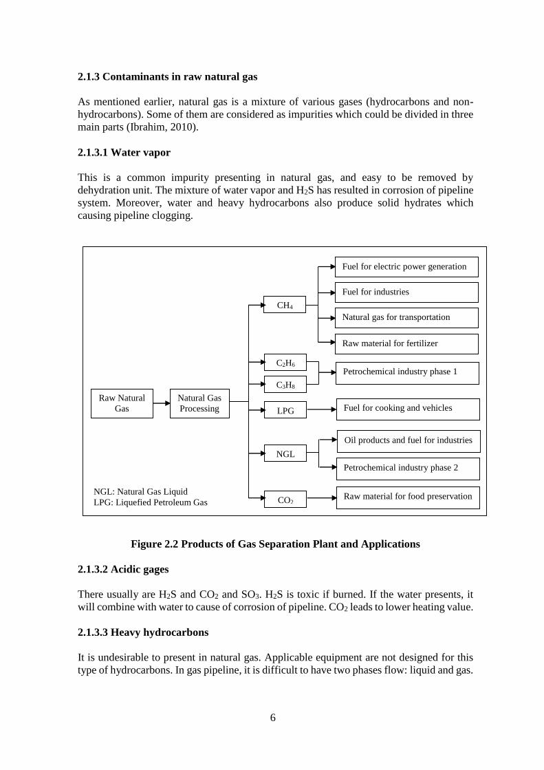
2.1.3 Contaminants in raw natural gas
As mentioned earlier, natural gas is a mixture of various gases (hydrocarbons and non-
hydrocarbons). Some of them are considered as impurities which could be divided in three
main parts (Ibrahim, 2010).
2.1.3.1 Water vapor
This is a common impurity presenting in natural gas, and easy to be removed by
dehydration unit. The mixture of water vapor and H2S has resulted in corrosion of pipeline
system. Moreover, water and heavy hydrocarbons also produce solid hydrates which
causing pipeline clogging.
Figure 2.2 Products of Gas Separation Plant and Applications
2.1.3.2 Acidic gages
There usually are H2S and CO2 and SO3. H2S is toxic if burned. If the water presents, it
will combine with water to cause of corrosion of pipeline. CO2 leads to lower heating value.
2.1.3.3 Heavy hydrocarbons
It is undesirable to present in natural gas. Applicable equipment are not designed for this
type of hydrocarbons. In gas pipeline, it is difficult to have two phases flow: liquid and gas.
Raw Natural
Gas
Natural Gas
Processing
C2H6
C3H8
Petrochemical industry phase 1
NGL
Oil products and fuel for industries
Petrochemical industry phase 2
Raw material for food preservation CO2
CH4
Fuel for electric power generation
Fuel for industries
Natural gas for transportation
Raw material for fertilizer
LPG Fuel for cooking and vehicles
NGL: Natural Gas Liquid
LPG: Liquefied Petroleum Gas
7
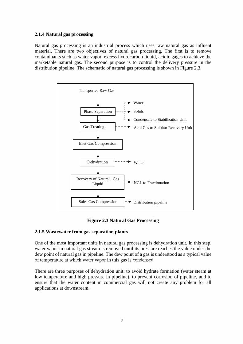
2.1.4 Natural gas processing
Natural gas processing is an industrial process which uses raw natural gas as influent
material. There are two objectives of natural gas processing. The first is to remove
contaminants such as water vapor, excess hydrocarbon liquid, acidic gages to achieve the
marketable natural gas. The second purpose is to control the delivery pressure in the
distribution pipeline. The schematic of natural gas processing is shown in Figure 2.3.
Figure 2.3 Natural Gas Processing
2.1.5 Wastewater from gas separation plants
One of the most important units in natural gas processing is dehydration unit. In this step,
water vapor in natural gas stream is removed until its pressure reaches the value under the
dew point of natural gas in pipeline. The dew point of a gas is understood as a typical value
of temperature at which water vapor in this gas is condensed.
There are three purposes of dehydration unit: to avoid hydrate formation (water steam at
low temperature and high pressure in pipeline), to prevent corrosion of pipeline, and to
ensure that the water content in commercial gas will not create any problem for all
applications at downstream.
Inlet Gas Compression
Dehydration
Recovery of Natural Gas
Liquid
Sales Gas Compression
Transported Raw Gas
Phase Separation
Gas Treating
Water
Solids
Condensate to Stabilization Unit
Acid Gas to Sulphur Recovery Unit
Water
NGL to Fractionation
Distribution pipeline
8
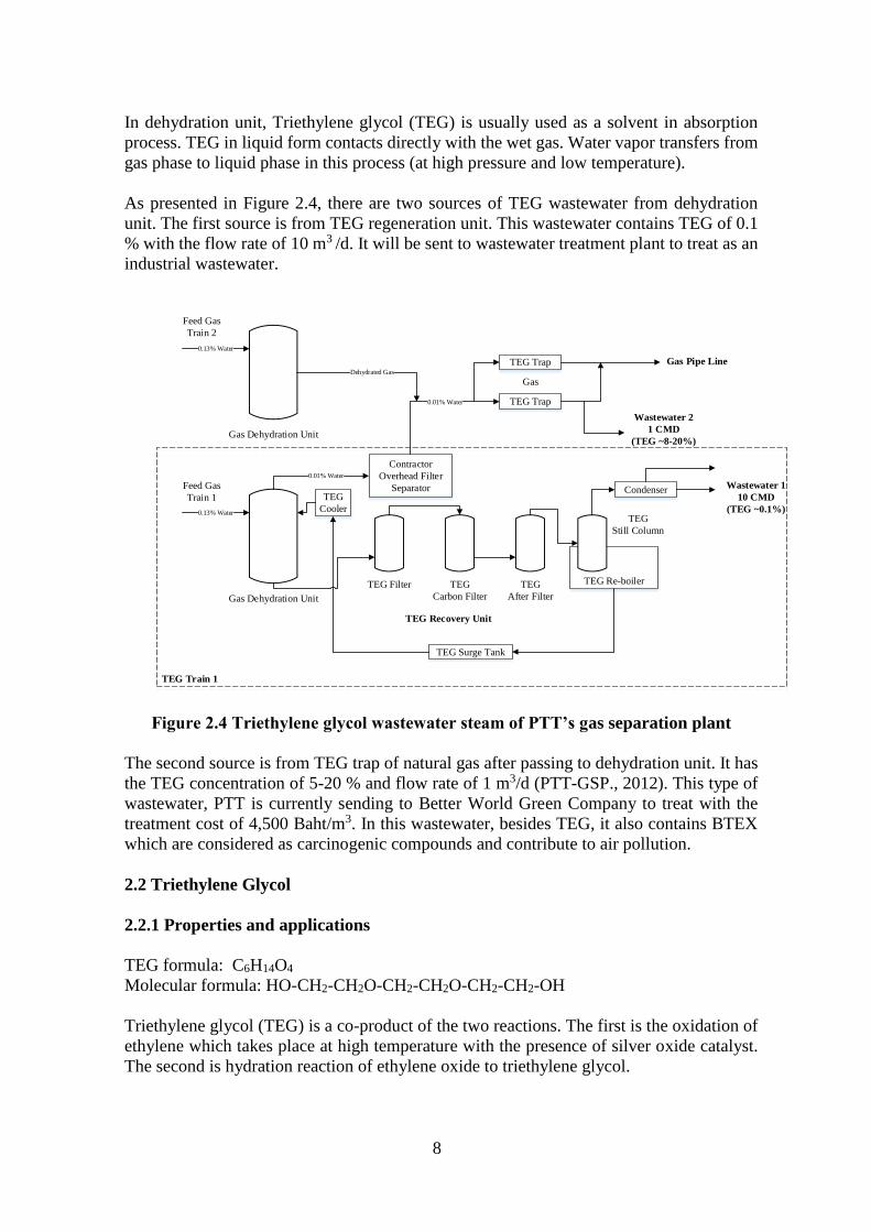
In dehydration unit, Triethylene glycol (TEG) is usually used as a solvent in absorption
process. TEG in liquid form contacts directly with the wet gas. Water vapor transfers from
gas phase to liquid phase in this process (at high pressure and low temperature).
As presented in Figure 2.4, there are two sources of TEG wastewater from dehydration
unit. The first source is from TEG regeneration unit. This wastewater contains TEG of 0.1
% with the flow rate of 10 m3 /d. It will be sent to wastewater treatment plant to treat as an
industrial wastewater.
TEG
Cooler
Gas Dehydration Unit
TEG Filter TEG
Carbon Filter
TEG
After Filter
TEG Re-boiler
TEG
Still Column
Condenser
TEG Surge Tank
Contractor
Overhead Filter
Separator
0.01% Water
Gas Dehydration Unit
TEG Trap
TEG Trap0.01% Water
Dehydrated Gas
0.13% Water
0.13% Water
Feed Gas
Train 2
Feed Gas
Train 1
Gas
Gas Pipe Line
Wastewater 2
1 CMD
(TEG ~8-20%)
Wastewater 1
10 CMD
(TEG ~0.1%)
TEG Train 1
TEG Recovery Unit
Figure 2.4 Triethylene glycol wastewater steam of PTT’s gas separation plant
The second source is from TEG trap of natural gas after passing to dehydration unit. It has
the TEG concentration of 5-20 % and flow rate of 1 m3/d (PTT-GSP., 2012). This type of
wastewater, PTT is currently sending to Better World Green Company to treat with the
treatment cost of 4,500 Baht/m3. In this wastewater, besides TEG, it also contains BTEX
which are considered as carcinogenic compounds and contribute to air pollution.
2.2 Triethylene Glycol
2.2.1 Properties and applications
TEG formula: C6H14O4
Molecular formula: HO-CH2-CH2O-CH2-CH2O-CH2-CH2-OH
Triethylene glycol (TEG) is a co-product of the two reactions. The first is the oxidation of
ethylene which takes place at high temperature with the presence of silver oxide catalyst.
The second is hydration reaction of ethylene oxide to triethylene glycol.

9
TEG is a transparent chemical which is colorless, low volatility, high viscosity and water
soluble. TEG is odorless at normal conditions and sweet at high vapor concentration. Its
properties are familiar with other glycols in hydroxyl group. However, it is preferential to
use TEG in some applications which require higher boiling point, higher viscosity, higher
molecular weight and lower volatility than other glycols. In all applications of TEG, the
solubility is the most important characteristics.
Table 2.3 Properties of Triethylene Glycol (Dow, 2014)
Property Units Value
Auto-ignition Temperature oC 349
Boiling Point at 760 mmHg oC 288
Freezing Point oC -4.3
Heat of Vaporization kJ/gmol 62.5
Molecular Weight g/mol 150.17
Specific Gravity at 20 oC - 1.1255
Viscosity at 20 oC mPs 49
Surface Tension mN/m 45.5
Vapor pressure at 20 oC kPa <0.001
Solubility of Water in Triethylene Glycol at 20°C wt% 100
Solubility in Water at 20°C wt% 100
Figure 2.5 Break down of TEG application in US (Dow, 2014)
Gas dehydration
54%
Solvent
10%
Plasticizer
11%
Polyurethanes
9%
Humectant
4%
Others
12%
10
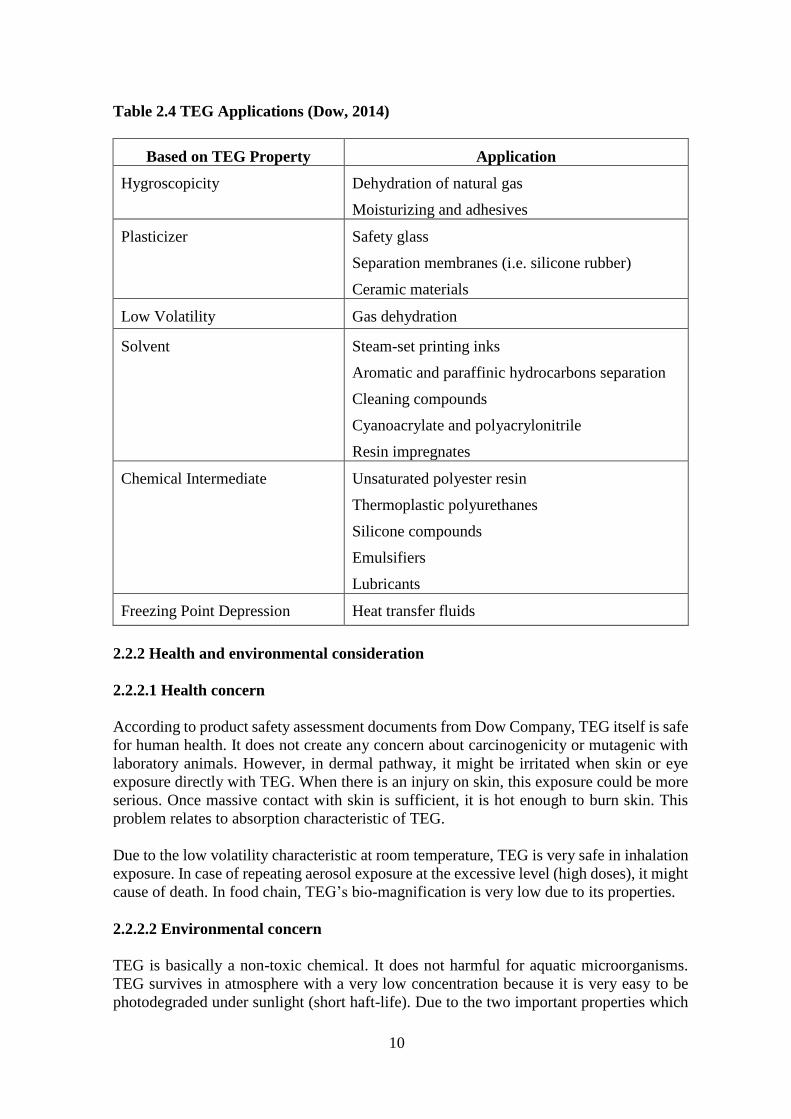
Table 2.4 TEG Applications (Dow, 2014)
Based on TEG Property Application
Hygroscopicity Dehydration of natural gas
Moisturizing and adhesives
Plasticizer Safety glass
Separation membranes (i.e. silicone rubber)
Ceramic materials
Low Volatility Gas dehydration
Solvent Steam-set printing inks
Aromatic and paraffinic hydrocarbons separation
Cleaning compounds
Cyanoacrylate and polyacrylonitrile
Resin impregnates
Chemical Intermediate Unsaturated polyester resin
Thermoplastic polyurethanes
Silicone compounds
Emulsifiers
Lubricants
Freezing Point Depression Heat transfer fluids
2.2.2 Health and environmental consideration
2.2.2.1 Health concern
According to product safety assessment documents from Dow Company, TEG itself is safe
for human health. It does not create any concern about carcinogenicity or mutagenic with
laboratory animals. However, in dermal pathway, it might be irritated when skin or eye
exposure directly with TEG. When there is an injury on skin, this exposure could be more
serious. Once massive contact with skin is sufficient, it is hot enough to burn skin. This
problem relates to absorption characteristic of TEG.
Due to the low volatility characteristic at room temperature, TEG is very safe in inhalation
exposure. In case of repeating aerosol exposure at the excessive level (high doses), it might
cause of death. In food chain, TEG’s bio-magnification is very low due to its properties.
2.2.2.2 Environmental concern
TEG is basically a non-toxic chemical. It does not harmful for aquatic microorganisms.
TEG survives in atmosphere with a very low concentration because it is very easy to be
photodegraded under sunlight (short haft-life). Due to the two important properties which
11
are soil mobility and biodegrades readily, TEG concentration in natural environment is
very low (Dow, 2014). Within 20 days, TEG can be degraded 90 % (measuring by BOD20).
2.2.3 TEG Recovery methods
In literature, amount of research on treatment of TEG wastewater is very less. However,
some authors had conducted their study on treatment and/or concentrate ethylene glycol
from wastewater. Evaporation process had proven as an effective method when it can
concentrate ethylene glycol up to 70 % (Jehle et al., 1995). Unfortunately, this is a very
slow treatment process and consume high energy. Thus, evaporation is not a really
promising process. Using nanofiltration (NF) process on concentrating ethylene glycol was
studied (Orecki et al., 2006). However, the rejection of NF membrane was failed in all tests.
2.2.3.1 Conventional membrane process
Larpkiattaworn (2013) studied about TEG removal by using polyethersulfone (PES-NTR
7450) membrane. From this study, 99 % TEG was rejected at the condition of feed
temperature 28oC and applied pressure of 1 kg/cm2.
By using two nanofiltration (NF) and two reverse osmosis (RO) membrane, Jacob (2014)
found out that the membrane’s selectivity were lost when the TEG concentration in feed
solution was higher than 10%. The author conducted the rejection test for both membranes.
The result of rejection examination of NF and RO were 80 and 83-95 % respectively. At
the initial concentration of TEG of 5%, the highest TEG concentration achieved was 89.12
and 95.74 % for RO-ACM5 and RO-NTR759 membranes respectively. The author had
concluded that membrane based treatment is effective only for wastewater that has low
initial TEG concentration (0.1-5%).
2.2.3.2 Distillation process
In the normal condition, the boiling point of water (100oC) is much lower than TEG
(288oC). Thus, by applying heat to TEG wastewater, water is first vaporized and be
collected. After dewatering step, heat is continuously applied until the temperature of waste
solution reaches the boiling point of TEG. Similar with dewatering process, TEG is distilled
and be collected. However, this process requires high energy.
2.2.3.3 Membrane distillation
Glycol separation had been studied in three configurations. The first study was conducted
with direct contact membrane distillation (DCMD) configuration by Rincón (1999).
Ethylene glycol could achieve 70% of concentration by using DCMD operating at
moderate temperature and atmospheric pressure. However, this mark was also the
limitation of DCMD. It could not achieve higher glycol concentration than that value. The
adverse effects of temperature and concentration polarization were a problem which a
careful attention must be paid to this issue. Using vacuum membrane distillation (VMD)
to concentrate ethylene glycol was studied by Mohammadi and Akbarabadi in 2005. These
authors concluded that ethylene glycol had ability to be recovered by VMD process. The
effectiveness of TEG rejection was achieved 100% in VMD configuration. However, VMD
consumes high energy than other membrane distillation configurations.
12
In membrane distillation process, it is certainly a need of an external energy source to heat
up the feed solution. Thus, optimizing energy consumption becomes attractive field for
further study.
Comparing between Distillation, NF/RO and MD
Since MD is the new technology which is not widely applied at industrial level, the
economic feasibility of MD has not been evaluated completely. To operate a MD system,
the basic standard of energy required is 628 kWh/m3 (Camacho et al., 2013) while the
energy consumption of water production required for a RO system is only 2.49 kWh/m3
(Liu et al., 2011)
Kesieme et al. (2013) conducted the study on a desalination plant that has a capacity of
30,000 m3/day with different technologies. The authors indicated that it is not economical
when comparing between MD and RO/MED if the plant is operated by supplied steam (in
this case, the production cost of MD, MED and RO are 1.72, 1.48 and 0.69 $/m3
respectively). However, the production cost of MD can reduce to 0.57 $/m3 by using waste
heat. Thus, MD would be the promising technology which against other conventional
processes.
2.3 Membrane Science and Technology
In the trend of development of water and wastewater treatment technology, membrane
technology had been developed and become important rapidly. This technology has many
potentialities to rationalize of operation process. The appearance of membrane technology
was to adapt the three important aspects: water scarcity (reclamation for water reuse),
regulatory pressure (stricter standards), and treatment cost improvement (economic
efficiency). In the field of environmental treatment, membrane technologies has been
increasingly applied exponentially within recently years (Metcaf, Eddy, 2003) and will
continue dramatically in the future.
In many places on over the world where water supplies are restricted of quantity and
quality, the concepts of reclamation, reuse and protection of water have been played a very
important role (Daigger et al., 2006) to reduce water footprint – an indicator for water reuse.
By using ultrafiltration (UF), Giardia and Cryptosporidium protozoa would be removed
(which conventional treatment process could not eliminate) completely. The strictness of
water standard (for both reuse and discharge) is rising along with timeline. For example,
nitrogen and phosphorus are required to reach the stringent standard before discharge to
reduce eutrophication phenomenon, by using membrane bioreactor (MBR), both biological
and chemical nitrogen can be removed successfully (Daigger, Crawford, 2005). From the
aspects of cost improvement, there are low cost in both membrane material (i.e. woven
fiber microfiltration (WFMF) (Thanh, Dan, 2013)) and treatment process by consuming
less energy, chemical, land use and labor while producing more water and remove more
impurities (zero discharge concept).
The main mechanism of membrane treatment is pore-filtration process, like a factitious
kidney, by providing physical barriers. From the difference in size of pores, there are
different applications and so that various materials are rejected by the pore on the surface
13
of membrane. The smaller of pore size, higher pressure of feed water needed to operate the
filtration process. Also, the properties of surface are very important. It is needed to provide
higher pressure for hydrophobic surface than hydrophilic. The typical membrane material
used for wastewater treatment is organic compound, includes: polypropylene, cellulose
acetate, aromatic, polyamides, and thin-film composites (TFC). By tailoring and adjusting,
membrane properties can be matched with any specific design of separation tank. It has
ability to upscale or connect with other treatment process to achieve higher efficiency.
However, there are also some disadvantages of membrane process, such as requirement of
chemical pretreatment or membrane fouling, and in operating process, it also can be
destroyed by incident or shock-loading. Overall characteristics of six membrane process
are shown in Table 2.5.
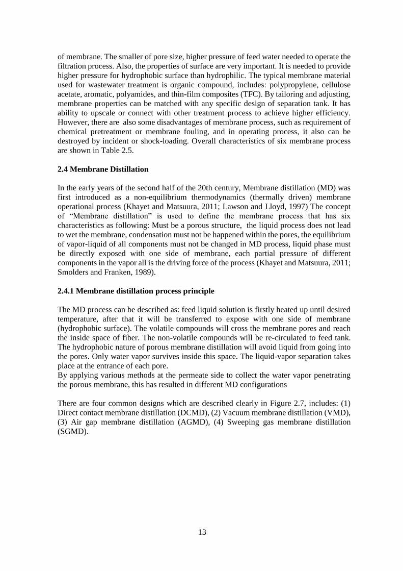
2.4 Membrane Distillation
In the early years of the second half of the 20th century, Membrane distillation (MD) was
first introduced as a non-equilibrium thermodynamics (thermally driven) membrane
operational process (Khayet and Matsuura, 2011; Lawson and Lloyd, 1997) The concept
of “Membrane distillation” is used to define the membrane process that has six
characteristics as following: Must be a porous structure, the liquid process does not lead
to wet the membrane, condensation must not be happened within the pores, the equilibrium
of vapor-liquid of all components must not be changed in MD process, liquid phase must
be directly exposed with one side of membrane, each partial pressure of different
components in the vapor all is the driving force of the process (Khayet and Matsuura, 2011;
Smolders and Franken, 1989).
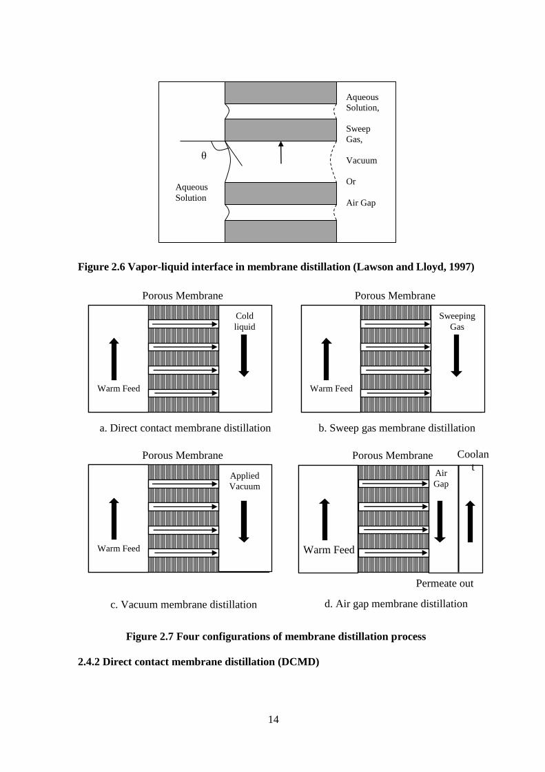
2.4.1 Membrane distillation process principle
The MD process can be described as: feed liquid solution is firstly heated up until desired
temperature, after that it will be transferred to expose with one side of membrane
(hydrophobic surface). The volatile compounds will cross the membrane pores and reach
the inside space of fiber. The non-volatile compounds will be re-circulated to feed tank.
The hydrophobic nature of porous membrane distillation will avoid liquid from going into
the pores. Only water vapor survives inside this space. The liquid-vapor separation takes
place at the entrance of each pore.
By applying various methods at the permeate side to collect the water vapor penetrating
the porous membrane, this has resulted in different MD configurations
There are four common designs which are described clearly in Figure 2.7, includes: (1)
Direct contact membrane distillation (DCMD), (2) Vacuum membrane distillation (VMD),
(3) Air gap membrane distillation (AGMD), (4) Sweeping gas membrane distillation
(SGMD).
14
Figure 2.6 Vapor-liquid interface in membrane distillation (Lawson and Lloyd, 1997)
Figure 2.7 Four configurations of membrane distillation process
2.4.2 Direct contact membrane distillation (DCMD)
Warm Feed
Cold
liquid
Porous Membrane
a. Direct contact membrane distillation
Warm Feed
Sweeping
Gas
Porous Membrane
b. Sweep gas membrane distillation
Warm Feed
Applied
Vacuum
Porous Membrane
Permeate out
Warm Feed
Porous Membrane
Air
Gap
Coolan
t
d. Air gap membrane distillation c. Vacuum membrane distillation
Aqueous
Solution
θ
Aqueous
Solution,
Sweep
Gas,
Vacuum
Or
Air Gap

15
In DCMD, condensing liquid solution with low temperature is used at the permeate side.
Both feed aqueous solution and permeate liquid solution are directly expose to the
membrane surface. The difference in temperature of the two liquid flows is the driving
force of this process. As a result, there are two interface at both sides of each pore, the
interface of vapor/hot aqueous at the entrance and vapor/cold at the permeate side. The
partial pressure of cold liquid at permeate side can be reduced to enhance the driving force
of DCMD by using osmosis distillation (OD) water (Laganà et al., 2000)
This configuration of MD is the most popular application to carry out the experiment
(Andrjesdóttir et al., 2013; Khayet and Matsuura, 2011; Phattaranawik and Jiraratananon,
2001; Qtaishat et al., 2008). For the separation of heated influent flow is water (desalination
or concentration of liquid solution), DCMD is the best solution (Laganà et al., 2000;
Lawson and Lloyd, 1997).
2.4.3 Vacuum membrane distillation (VMD)
In VMD configuration, a vacuum pump is used to maintain vacuum condition at the
downstream side of the membrane. The saturation pressure of volatile material that needed
to be separated must be higher than vacuum pressure (Khayet and Matsuura, 2011; Lawson
and Lloyd, 1997). The driving force of VMD processing is the difference in the pressure
between two sides or each pore. Comparing the permeate flux of RO and four
configurations of MD, VMD provided highest value. This result is achieved due to reducing
downstream pressure (Bandini et al., 1992; Izquierdo-Gil, Jonsson, 2003). However, the
main adverse point of VMD is the great opportunity of pore wetting due to the negative
pressure at the permeate side of membrane. Hence, VMD will operate better with the
smaller pore size (Khayet and Matsuura, 2011; Lawson and Lloyd, 1997).
The applications of VMD is described clearly by (Sarbatly and Chiam, 2013), includes:
Desalination (NaCl/water), concentration (LiBr/water), extraction of trace volatile organic
compounds (ethanol/water), removal of dissolved gases (Ammonia/water), preservation of
aroma compounds (Must/aromas/water), recovery of aroma compounds (blackcurrant
aromas).
2.4.4 Air gap membrane distillation (AGMD)
In AGMD, only one side of MD is exposed with feed heated aqueous solution, the
remaining side is unattached (Meindersma et al., 2006). Between the permeate side of
membrane surface and the surface of condensation, a stagnant air gap is located. Before
condensing at the cold condenser, the vapor of volatile material has already been passed
both the porous structure membrane and air gap (El-Bourawi et al., 2006; Khayet and
Matsuura, 2011). So, AGMD produced a lowest permeate flux in comparison with other
configurations of MD.

16
Table 2.5 General Characteristics of Membrane Process (Metcalf and Eddy, 2004)
Membrane
process
Membrane
driving force
Typical
separation
mechanism
Operating
structure
(pore size)
Typical
operating
range (µm)
Permeate
description
Typical constituents
removed
Microfiltration
(MF)
Hydrostatic
pressure difference
of vacuum in open
vessels
Sieve Macropores
(>50 nm) 0.08-2.0
Water,
dissolved solutes
TSS, turbidity,
protozoan oocysts and
cysts, some bacteria and
viruses
Ultrafiltration
(UF)
Hydrostatic
pressure difference Sieve
Mesopores
(2-50 nm) 0.005-0.2
Water; small
molecules
Macromolecules,
colloids, most bacteria,
some viruses, proteins
Nano filtration
(NF)
Hydrostatic
pressure difference
Sieve + solution/
diffusion +
exclusion
Micropores
(<2nm) 0.001-0.01
Water, very
small molecules,
ionic solutes
Small molecules, some
hardness, viruses
Reverse osmosis
(RO)
Hydrostatic
pressure difference
Solution /
diffusion +
exclusion
Dense
(<2nm) 0.0001-0.001
Water, very
small molecules,
ionic solutes
Very small molecules,
color, hardness, sulfate,
nitrate, sodium, other
ions
Dialysis Concentration
difference Diffusion
Mesopores
(2-50 nm) -
Water; small
molecules
Macromolecules,
colloids, most bacteria,
some viruses, proteins
Electro- dialysis
Electromotive force
Ion exchange
with selective
membranes
Micropores
(<2nm) -
Water, ionic
solutes Ionized salt ions
17
The gas between membrane surface and cold surface is a barrier that resulted in reduction
of head loss (Meindersma et al., 2006). The vapor flux has to be maintained to overcome
the air gap barrier. This flux is affected by the width of air gap.
Air gap membrane distillation is suitable for seperation of alcohols/liquid solution (Garcı́a-
Payo et al., 2000). This separation could not be implemented by DCMD because volatiled
alcohol is probable to wet the pore at permeate side because of lower surface tension
(Meindersma et al., 2006).
2.4.5 Sweeping gas membrane distillation (SGMD)
SGMD has another name as membrane air stripping (Meindersma et al., 2006). Similar
with VMD, vapor is condensed at the place outside membrane module. The mechanism of
this process operation is the removal of vapor by a sweep gas at the permeate side of
membrane. In SGMD, the advantage is the small resistance of air barrier that affected to
mass transfer. However, the vapor will be diluted in sweep gas that resulted in requirement
of higher condenser capacity. Furthermore, sweeping gas is easily and fast heated up by
the temperature from the vapor. Consequently, the vapor pressure would be increased to
higher level which has resulted in reducing the driving force of this operating process. In
this MD configuration, the flux is not depend of the temperature of the gas (Lawson, Lloyd,
1997). Similar with AGMD, SGMD is mostly used to remove volatile compound more than
water (Khayet and Matsuura, 2011; Zhang et al., 2000).
2.5 Material of Membrane and Module Fabrications Using for Distillation Process
The selection of MD is depended on each typical required application. It is a combination
of permeate flux, thermal conductivity, pore size, porosity, separation factor (Khayet,
2011).
2.5.1 Commercial membranes used in distillation process
To prevent the membrane wetting phenomena, hydrophobic polymer is an appropriate
material for this micro-porous membrane. Many different polymers could be used, such as:
Polypropylen, Polyvinylidene fluoride, polythylene, polytetrafluoroethylene with the
abbreviated forms as PP, PVDF, PE, PTEE respectively. These material are survived in
various shapes, such as: tubular, capillary, flat sheet. The morphological configurations of
these synthetic materials are close to meet all requirements of MD process.
2.5.2 Fabricated membranes for distillation Process
Based on different materials, various hydrophobic porous membranes are created by using
diverse techniques. The choice and production are relied on various factors, includes:
aqueous solution, range of temperature that MD can operate with, thermal conductivity,
price, easy or difficult to fabricate and assembly. Flat sheet, hollow fiber with single
hydrophobic layer membrane and composite multilayers membrane (bi-layer of
hydrophobic/hydrophilic membrane) are created and used (Khayet, 2011).
2.5.2.1 Flat sheet and frame module
18
Many types of flat sheet membranes with single hydrophobic layer have been developed
and applied for MD processing, such as: asymmetric PVDF (polymer concentration of 10-
25wt.%, solvent used of 13.2 -15 wt.% , porosity >79%, pore size of 0.0698-0.349 µm),
copolymer PVDF-TFE (pore size < 2.4 x10⁻² µm, porosity < 80 %), copolymer PVDF-HFP
(19.1 wt.% PVDF-HFP, solvent polyethylene glycol (PEG) of 4.99 wt.%) (Khayet and
Matsuura, 2011).
Depends on each membrane that has different concentration of polymer and using different
amount of solvent, there will be the difference in the maximum coefficient of mass transfer
of different membranes. This module is generally used in laboratory studies because it can
be cleaned and replaced easily. Notwithstanding, it is very low in the value of the ratio
between area of membrane to the module volume.
2.5.2.2 Hollow fiber module
By using different polymers, different solvents and different spinning process (dry/wet),
the different hollow fiber membrane were made out. Some common materials for hollow
fiber are: PVDF, PVDF/Cloisite clay, PTFE, copolymers (Khayet, 2011). An typical
example, PVDF membrane material with pore size of 4.0-24.8 nm, porosity of 56-73 %,
internal diameter of 0.675-0.844 mm, external diameter of 0.982-1.071 mm (Fujii et al.,
1992).
The main composition of this module is a shell tube that includes a determined number of
hollow fibers bundled and sealed. The significant advantages of this type of module are
low energy consumption and high membrane area in a limited volume. Contrarily, it is
difficult to clean and high opportunity to get fouling.
2.5.2.3 Spiral wound module
The components of this type include a flat sheet membrane that is rolled and enveloped in
a limited space. The center of the winding is a collection pipe. The movement of feed
solution overpass the membrane surface is in an axial trend while the permeate flux goes
into the central tube. Alkhudhiri (2012) confirmed that this module has high packing
density, not easy to fouling, and the energy consumption is acceptable.
2.6 Operational Processes of Membrane Distillation
2.6.1 Development of theoretical models for membrane distillation
One side of membrane must be directly contact with the feed heated aqueous solution. The
membrane aqueous solution entry pressure (liquid entry pressure – LEP) must be higher
than the applied hydrostatic trans-membrane pressure. The surface tension force of
membrane (hydrophobic nature) prevents liquid from entering the pores. Generally, there
is a supposition of the negligible kinetic effect of liquid/vapor interface and the equilibrium
of liquid/vapor phases is directly corresponding to the temperature at membrane surfaces
when developing a MD model process (Khayet, 2011).
The formula is used to calculate separation factor for the feed solution containing non-
volatile materials is as following:
19
α = (1 −Cp
Cf) 100 (2.5)
Where α is the separator factor, 𝐶𝑝 is the solute concentration in the permeate flux and 𝐶𝑓
is the concentration in feed flow.
If the volatile compounds are contained in feed solutions, the above formula will be
changed to:
α =Xv,p/Xw,p
Xv,f/Xw,f (2.6)
With X𝑣,𝑝, X𝑤,𝑝are the mole fractions of volatile compounds (v), water (w) in the permeate
(p) flux and X𝑤,𝑝, X𝑤,𝑓 are those values in feed (f) solutions.
The vapor pressure of a given compound (i) is calculated by Antoine Equation as following:
pi(T) = exp (α −β
γ+T) (2.7)
Where pi and T are the partial vapor pressure of the pure component in the permeate flux
(Pa) and absolute temperature (K), α, β, γ are constants that depend on typical material. i
can be water or any chemical compound (for water, α = 23.1964, β =3816.44, γ = - 46.13).
By calculating the condensate collected in the permeate side of MD module for a
determined time, the permeate flux (Ji) in all MD configurations (that depends on the nature
characteristics of membrane and driving force) would be measured
Jw = Bw∆pw = Bw(p𝑚,𝑓 − p𝑚,𝑝) (2.8)
Where J is kg/m2h, , Bw is the membrane coefficient (permeability of MD), p𝑚,𝑓 is the
partial vapor pressure of water in the feed solution, p𝑚,𝑝 is its value in permeate side.
If the feed solution is diluted aqueous of non-volatile materials, the partial vapor pressure
of that solution can be calculated as:
pw,s = (1 − xs)pw (2.9)
With pw,s is the vapor pressure of a diluted aqueous of non-volatile materials, pw is the
vapor pressure of water, xs is the mole fraction of non-volatile compound.
Liquid entry pressure
The concept of liquid entry pressure (LEP) is used to prevent the wetting phenomenon of
membrane pores. LED is the lowest pressure that needs to be applied for the feed aqueous
solution before touching the entrance of the dry pores. The value of LEP can be measured
by using the Laplace Equation (Lawson, Lloyd, 1997) which is expressed as the following:
20
LEP > ∆Pinterfae = Pliquid − Pvapor =−2BγL cos θ
rmax (2.10)
Where , B, γL, θ, rmax are geometric coefficient which is measured by pore structure,
aqueous surface tension, the angle of the contact between liquid and solid (feed aqueous
solution and the surface of membrane), and the largest pore size respectively. In general,
VMD uses the membrane which has rmax < 0.45 µ𝑚 (Lawson, Lloyd, 1997). The value
of LEP reduces along with the increase of rmax of membrane and/or the reduction of θ.
2.6.2 Mass transfer in membrane distillation
There are two contingents of mass transfer through MD. One part is volatile compounds in
vapor will cross the pores of MD then it will pass the boundary layers of membrane surface
in the second part. This layer is a thin film between membrane surface and bulk aqueous
solution and will be discussed in details in the polarization section.
The permeate flux which is through the micro-porous membrane can be anticipated exactly
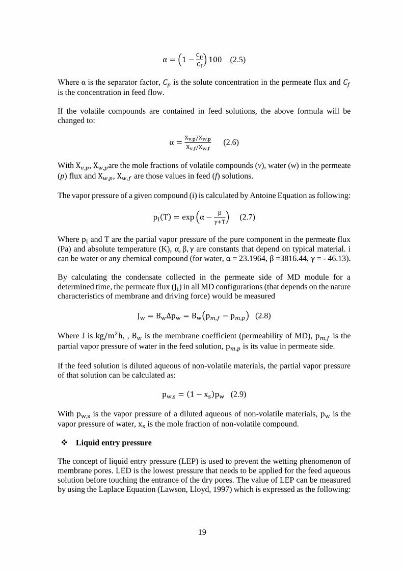
by using dusty gas model. This model is the combination of four componential
mechanisms: Knudsen diffusion, ordinary molecular diffusion, viscous/poiseuille of flow
(surface diffusion is neglected in dusty model) (Khayet and Matsuura, 2011). The typical
expression is shown in Figure 2.8.
Dusty gas model
In water, the solubility of air is about 10 ppm (Khayet, 2011). Generally, mass transfer in
MD is the results of convective and diffusion of volatile material which cross the pores of
membrane. Knudsen diffusion model and Viscous/Poiseuille model are used to describe
the resistance of micro-porous structure membrane in absence of air. Molecular diffusion
model is used to describe the mass flux in presence of air. In dusty gas model that using for
DCMD, surface diffusion is considered as neglect due to the very small membrane surface
in comparison with the total area of pores. Besides, the operating pressure of DCMD is
always maintained at a constant value (~105 Pa) and the flow of vapor that passing the
membrane porous is very small relative to the water flux, thus viscous flow is not
considered as significantly negligible (Lawson and Lloyd, 1997).
Knudsen number (Kn) is the quantifiable value which is used to determine the operational
mechanism of a pore of MD under a typical condition. This number is calculated as a ratio
of the mean free path (λ) of a given compound (the mean free path can be defined as the
average route of a moving molecule between each successful collision)n. This collision
must change directly energy or direction of that molecule) to the pore size MD (dp).
Kn =λ
dp (2.11)
The value of mean free path of a given molecules (λi, m) can be measured by using the
following Equation:
λi =Tkb
(√2)Pm(σi)2 (2.12)
21
Where σi is the collision diameter of given specie (for water molecules in gas phase, σw =2.641 × 10⁻¹⁰ m), kb is Boltzmann constant, Pm is the mean pressure within the pores,
and T is the absolute temperature.
Figure 2.8 Dusty gas model
Membrane distillation coefficient is calculated by Equation 2.13.
Bik =
2πrk3
3RTτδ (
8RT
πMi)
12⁄
(2.13)
Where 𝑟𝑘, 𝑀𝑖, 𝛿, 𝜏, 𝑅 are pore radius of membrane, molecular weight of given specie,
thickness of membrane, tortuosity of membrane and gas constant respectively.
In case Kn < 0.1 (dp > 10λi) , molecular-molecular impinge (molecular diffusion) is the
main responsibility for mass transfer the pressure of MD operating system in this situation
is nearly approximate to atmospheric pressure (Qtaishat et al., 2008). The Equation 2.14
below expresses the membrane coefficient of MD that has a pore’s area of 𝜋𝑟𝐷2 in the
region of ordinary diffusion model.
BiD =
πPDirD2
RTPaτδ (2.14)
Where Pa is the partial pressure of vapor inside the pore, P is total pressure within the
membrane pore, Di is the diffusion coefficient of a given material.
For air/water solutions, PDi can be measured by the Equation below where PDw value is
expressed in the unit of Pa m2 s⁄
PDw = 1.895 × 10⁻⁵ × T2.072 (2.15)
If the value of Kn is in the range from 0.01 to 1 (100λi > dp > λi), the transportation
mechanisms of given volatile compounds are molecule-wall and molecule-molecule
diffusion (Knudsen and ordinary diffusion) which are taking place in combination. Micro-
porous membrane’s permeability of the pores that has an area of 𝜋𝑟𝑡2 can be calculated by
using Equation 2.16.
Knudsen Ordinary diffusion
Rv = 0
Viscous
Rs = 0
Surface

22
BiC =
π
RTτδ[(
2
3rt
3 (8RT
πMi)
12⁄
)
−1
+ (PDirt
2
Pa)
−1
]
−1
(2.16)
Khayet (2011) indicated that the combined Knudsen/molecular diffusion mechanism is
dominant for the membranes which has pore sizes in the range from 0.2 to 1 µm. When the
mean free path is close to to the mean pore size, permeate flux will not increase along with
the opening of pore size. Consequently, MD will work better with the membrane that has
smaller pore size than the mean free path (achieving higher flux under Knudsen diffusion
mechanism)
Khayet and Matsuura (2011) found that the mechanism responds for water vapor across
the pores of membrane is the combination of Knudsen diffusion and molecular diffusive
flux. The total permeate flux can be presaged exactly by theoretical model, but it is over
ability to estimate the partial organic permeate flux.
The partial pressure of water vapor (pw,p) in the permeate flux at the permeate side can be
calculated by using the formula as below:
pw,p =P.w
w+0.622 (2.17)
Where P is the total pressure of permeate flux at the permeate side, w is the humidity ratio.
The value of pw,p is depended on the gas temperature at the surface of micro-porous
membrane.
The humidity ratio is determined for a typical given air sample, can be understood as a
portion of mass between water vapor and dry air. The value of w can be achieved by the
relation as following:
w = win +AJw
ma (2.18)
In the Equation above, win is the ratio of humidity at the inlet point of module, ma is the
air flow rate, A is membrane effective area, Jw is the total permeate flux achieved in SGMD
configuration.
The second-level formula for the permeate flux of water vapor is the combination of some
equations that presented as above.
Jw2 + Jwb + c = 0 (2.19)
The value of b and c (coefficients) are estimated from the following respectively:
b = Bw(P − awpw,f0 ) +
ma
A(win + 0.622) (2.20)
c = Bw
Ama (Pwin − awpw,f
0 (win + 0.622)) (2.21)

23
Where 𝑝𝑤,𝑓0 is partial pressure of pure water in permeate flux, aw is the activity of water,
𝐵𝑤 is the coefficient of SGMD (permeability, productivity).
If there is a mixture of specie i and j in the permeate vapor through the membrane pores,
the mean free path can be measured by the Equation as following:
λi/j =TKB
πPm(√1+Mi Mj⁄ )((σi+σj) 2⁄ )2 (2.22)
Where σi, σj and Mi, Mj are collision diameters and molecular weight of species i and j
(volatile compounds) respectively.
Once the mean free path of given molecules is shorter than the pore size of MD, molecule-
molecule collisions will become the main phenomenon for mass transfer, over the
molecule-wall collisions. Poiseuille (viscous) type of flow is the main mechanism in this
case. Consequently, Bi is evaluated by Equation 2.23:
Bi =εr2Pm
8τδniRT (2.23)
Where 𝑛𝑖, 휀 and P are viscosity of typical materials, porosity of membrane, and average
hydrostatic pressure within the pores respectively.
Figure 2.9 Poiseuille type of flow inside a pore of SGMD process
2.6.3 Heat transfer in membrane distillation
Membrane distillation process is operated by the combination of two processes: mass and
heat transfer process, which are happened simultaneously. The heat transfer in MD process
can be separated in three steps: (i) heat transfer cross the boundary layer at the feed side of
membrane surface, (ii) heat transfer throughout the pores of micro-porous membrane, (iii)
heat transfer cross the boundary layer at the permeate side of membrane surface. Figure
below divided total heat flux (𝑄𝑚) into two heat transfer mechanisms: (i) heat transfer

24
through membrane material (membrane wall) and heat of pores that filled up by gas (Qc)
and (ii) heat of volatile molecules in vapor flux (Qv).
Heat transfer at the two boundary layers which are feed side (Qf) and permeate side (Qp)
of membrane surfaces respectively as the following:
Qf = hf(Tb,f − Tm,f) (2.24)
Qp = hp(Tm,p − Tb,p) (2.25)
Where hf and hp are coefficients of heat transport though two boundary layers which are
mentioned above. The acronyms Tb,f, Tm,f, Tm,p, Tb,p in two equations above are
temperatures at bulk feed, membrane-feed (membrane-solution) interface, membrane-
permeate interface, bulk-permeate (vapor-liquid) interface respectively.
For the heat flux that transferring through membrane material (Qc) and heat trapped in the
vaporized molecules (Qv) (Qv can be understood by heat transfer accompanies with mass
transfer), its balance is performed as following:
Qm = Qc + Qv (2.26)
Two partial heat transfers above are expressed as the two following Equations:
Qv = Ji∆Hv,i (2.27)
Qc =km
δ(Tm,f − Tm,p) = hm(Tm,f − Tm,p) (2.28)
Where Ji, ∆Hv,i, km, hm, δ are permeate flux, latent heat of vapor molecules of specie i,
thermal conductivity of micro-porous MD, heat transfer coefficient of the whole
membrane, membrane thickness respectively.
The heat transfer coefficient of only vapor flux (hv) is measured as:
hv =Ji∆Hv,i
(Tm,f−Tm,p) (2.29)
Khayet (2011) indicated that 50-80 % of energy consumption is accounted for Qv, the
residual part is for Qc and Qc is considered as head loss. The efficiency of heat transfer (η)
is calculated by the Equation below:
η =Qv
Qc+Qv=
Ji∆Hv,i
Ji∆Hv,i+hm(Tm,f−Tm,p) (2.30)
In the stable condition:
Qf = Qm = Qp = Q (2.31)
25
So, the heat transfer process in MD (boundary layer at feet side – membrane material –
boundary layer at permeate side) can be expressed in the summary in the following
Equation:
hf(Tb,f − Tm,f) =km
δ(Tm,f − Tm,p) + Ji∆Hv,i = hp(Tm,p − Tb,p) = hc(Tb,f − Tb,p)
(2.31)
And
Q = ∆T [1
hf+
1
hp+
1
km δ⁄ +Ji∆Hv,i ∆Tm⁄]
−1
= ∆Thc (2.32)
With
hc = [1
hf+
1
hp+
1
km δ⁄ +Ji∆Hv,i ∆Tm⁄]
−1
(2.33)
Where ℎ𝑐 is the heat transfer coefficient of the whole MD process, ∆T (∆T = Tb,f − Tb,p)
is the bulk temperature disparity between feed aqueous solution and permeate flux, and
∆Tm (∆Tm = Tm,f − Tm,p) is the disparity of transmembrane temperature.
2.7 Temperature Polarization
Boundary layers are the limiting barriers of MD efficiency in the heat transfer process. To
quantify the size of partial resistance of the boundary layers over the total resistance of
whole heat transfer process, temperature polarization coefficient (TPC) is usually used.
TPC performs the driving force reduction (∆pi) and is calculated by the following
Equation:
TPC =Tm,f−Tm,p
Tb,f−Tb,p=
1
1+hc h⁄= 1 − hc h⁄ (2.34)
Where
h = (1
hf+
1
hp)
−1
(2.35)
According to Khayet (2011), TPC indicates whether MD design is good or not good. In
case of TPC smaller than 0.2, MD process is limited in heat transfer and very poor in
module design. If TPC is higher than 0.6, MD process is limited in mass transfer and poor
in productivity (low permeability).
If TPC is approximately close to 1, the heat transfer across both layers achieves a high
efficiency and the effect of thermal polarization is neglected and MD process is controlled
by resistance of mass transfer. If TPC is close to 0, the efficiency of heat transfer through
both layers is very low, the effect of thermal polarization is very high and MD process is
controlled by resistance of heat transfer. The desired MD system has the TPC value in the
range from 0.4 to 0.7. In other words, the difference of temperature at permeate boundary
layer from feed aqueous boundary layer is between 30% and 60%. TPC value can be
increased by increasing feed aqueous solution and permeate flow rate and decreases
temperature of feed solution.

26
TPC can be understood by the relation in the following Equations:
TPC = TPCf + TPCp − 1 (2.36)
TPCf = 1 −hc
hf=
Tm,f−Tb,p
Tb,f−Tb,p (2.37)
TPCp = 1 −hc
hp=
Tb,f−Tm,p
Tb,f−Tb,p (2.38)
Where TPCf and TPCp are heat polarization coefficients of feed and permeate flux. The
value of hf is always higher than hp (Khayet et al., 2002).
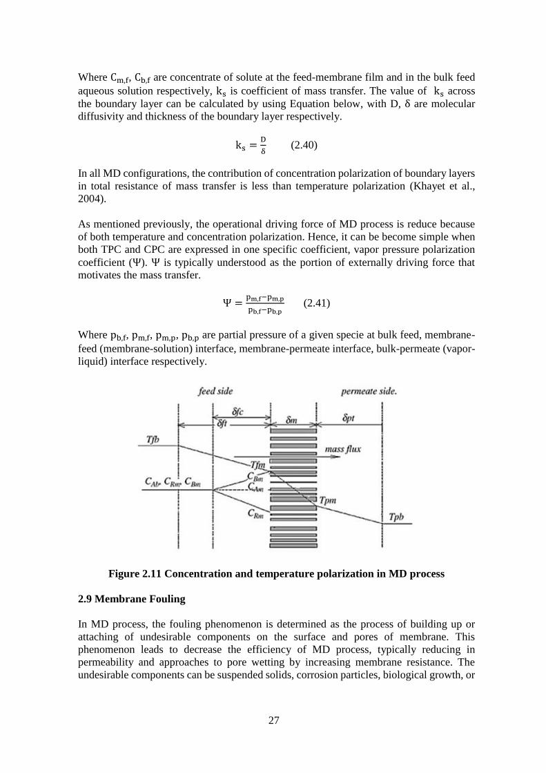
Figure 2.10 Temperature and concentration profile in MD process
2.8 Concentration polarization
In MD operational process, volatile solutes pass the membrane pores and micro-porous
membrane rejects non-volatile material, concentrating it on the membrane surface at the
feed side. The concentration of non-volatile compounds at the interface of membrane-feed
aqueous is higher than that in the bulk solution. Consequently, driving force of MD process
and permeate flux are reduced.
The value of concentration polarization coefficient (CPCi) of a given non-volatile
compound appear in feed solution is calculated as:
CPCi =Cm,f
Cb,f= exp (Jw ks⁄ ) (2.39)
Temperature
Concentration
Membrane
Boundary layer Boundary layer
Permeate Feed
27
Where Cm,f, Cb,f are concentrate of solute at the feed-membrane film and in the bulk feed
aqueous solution respectively, ks is coefficient of mass transfer. The value of ks across
the boundary layer can be calculated by using Equation below, with D, δ are molecular
diffusivity and thickness of the boundary layer respectively.
ks =D
δ (2.40)
In all MD configurations, the contribution of concentration polarization of boundary layers
in total resistance of mass transfer is less than temperature polarization (Khayet et al.,
2004).
As mentioned previously, the operational driving force of MD process is reduce because
of both temperature and concentration polarization. Hence, it can be become simple when
both TPC and CPC are expressed in one specific coefficient, vapor pressure polarization
coefficient (Ψ). Ψ is typically understood as the portion of externally driving force that
motivates the mass transfer.
Ψ =pm,f−pm,p
pb,f−pb,p (2.41)
Where pb,f, pm,f, pm,p, pb,p are partial pressure of a given specie at bulk feed, membrane-
feed (membrane-solution) interface, membrane-permeate interface, bulk-permeate (vapor-
liquid) interface respectively.
Figure 2.11 Concentration and temperature polarization in MD process
2.9 Membrane Fouling
In MD process, the fouling phenomenon is determined as the process of building up or
attaching of undesirable components on the surface and pores of membrane. This
phenomenon leads to decrease the efficiency of MD process, typically reducing in
permeability and approaches to pore wetting by increasing membrane resistance. The
undesirable components can be suspended solids, corrosion particles, biological growth, or

28
crystalline deposits. Once the fouling layer appears on the membrane surface, the thermal
resistance is also created. It leads to change the overall coefficient of heat transfer.
Fouling in MD process is not serious as others membrane separation process and it is easy
to overcome by some simple pre-treatment steps (Srisurichan et al., 2005). Alklaibi and
Lior (2005) concluded that the permeate flux can be enhanced up to 25% if the pre-
treatment process is implemented well. In another hand, this operational problem also can
be overcome by increasing the flow rate of feed solution and decrease the feed temperature
(Alkhudhiri et al., 2012).
2.9.1 Biological growth fouling
Some microorganisms grow and attach to the surface of membrane. The microorganisms
can be algae, bacteria, seaweed and fungi. Once this phenomenon takes place, a
significantly decline in permeate flux is happened together because of scale formation.
Biological growth can be reduced or prevented by boiling feed solution about half an hour
then filtrate this solution by appropriate filtration technology (El-Bourawi et al., 2006)
Figure 2.12 Profile of temperature in fouling case
2.9.2 Suspended particles and corrosion products fouling
The accumulation of suspended particles on the membrane surface is determined as
particulate fouling. There is always an approach of particles accumulation on the membrane
surface once the feed solution travels in MD system as streamline formation and the
random motion of particles leads to reach the gradient of undesirable component
concentration. Brownian diffusion affects directly on the travelling process of a very small
particles while the momentum forces control the large particles. Moreover, membrane
pores can be plugged by the particles that have sources from the corrosion of the equipment
Temperature
Thermal
Boundary layer
Fouling Layer
Membrane
Thermal
Boundary layer
29
such as pipe line, pump or heat exchangers. It is not able to predict when the fouling
phenomenon takes place because it is a time dependent process
2.9.3 Crystallization fouling
During the desalination process, the major operational problem of this MD application is
membrane surface is scaled by crystalline deposits formation, typically salt molecules. This
phenomenon leads to reduce the hydrophobicity of membrane and the pores can be clogged
by water. Karakulski (2002) found that the permeate flux is decreased dramatically when
CaCO3 accumulates on the membrane surface during the study about demineralization in
tap water. It is worth quoting here that crystal fouling formation is undetected in AGMD
module even this system was operated in a long period ( almost 2 month) (Banat, Simandl,
1994). This fouling is generally observed in DCMD process (Tun et al., 2005). It is mainly
related to salt solubility characteristics (which is usually decreased along with the reduction
of temperature).
The hydrodynamic condition and the interaction between membrane surface and foulants
were the most important factors affecting on membrane fouling. There were three types of
fouling: organic, inorganic, and biological fouling. In organic fouling, proteins tend to
attach on membrane hydrophobic surface. This has resulted in decreasing water contact
angle on membrane surface (membrane hydrophilization). In inorganic fouling
(crystallization fouling), it is not a significant problem due to the turbulent condition of
feed flow. About the biological fouling, because of the severe conditions of feed solution
in MD process (temperature and flow rate), biofilm could not be formed on the membrane
surface. Thus, the contribution of biofouling into the total membrane fouling is same with
inorganic fouling.
2.10 Membrane Cleaning
There are two adverse effects of membrane fouling: decreasing in permeate flux and
reducing membrane selectivity (due to reducing in hydrophobic nature of membrane). The
purposes of membrane cleaning process are to remove membrane fouling layers and
recover membrane properties. By applying an appropriate pre-treatment process,
membrane fouling can be reduced. Furthermore, cleaning of MD module can help to
restore membrane properties till its initial level. Reversible fouling can be removed by
clean membrane with pure water. Chemical cleaning can help to eliminate irreversible
fouling.
Guillen-Burrieza (2014) had conducted a study about various MD cleaning strategies in
term of permeate flux recovery, quality of distillation and membrane damage. There was a
difference in chemical solution used in this research. The author found out that the most
effective chemical using to clean MD membrane were the mixture of 0.1 wt.% Oxalic acid
and 0.8 wt.% Citric acid. The cleaning procedure using in this study were: 6 h with
chemical, 30 min with pure water and 24 h of dry-out.
2.11 Operating Variables Affecting MD Process
Variable factors affecting on the MD processing in each MD configuration are shown in
Table 2.6.
30
2.11.1 Effects of the temperature of feed solution
In general, the feed liquid solution is heated up till the range from 20 to 80oC (under the
level of boiling point) while all other parameters of MD are kept constant. From Table 2.6,
it is observed that accompanying with the increasing temperature of feed solution, MD flux
also increase exponentially.
This phenomenon can be explained by the increase of vapor pressure in aqueous solution
exponentially (which leads to increase driving force of MD process) with increasing
temperature. It is noticed that MD system is operating better when working under high
temperature of feed solution. Although the thermal polarization effect becomes higher
when increasing feed temperature but the contribution of feed temperature to evaporation
and total heat transfer is very high (El-Bourawi et al., 2006; J. Phattaranawik et al., 2003).
2.11.2 Effects of feed concentration
The effects of concentration of a typical solute in feed liquid on vapor flux strongly depend
on the separation process of that self-compound. MD process can be applied to treat feed
solution which is very high concentration in comparison with other conventional membrane
process (which is operated by pressure-driven) (Banat, Simandl, 1994).
While considering non-volatile compounds in feed solution, it was found that the main
effect of itself is the reducing in vapor flux of MD processing. Consequently, it was
concluded that the driving force of MD separation process can be reduced by adding non-
volatile compound to feed solution (by decreasing partial vapor pressure). The effects of
concentration polarization also get the contribution from that (increases the thickness of
boundary layer on feed side of MD) (Tomaszewska et al., 1998)
When volatile solutes in feed solution (i.e. alcohols, ammonia) are considered, it was found
that the permeate flux would be increased when rising the volatile components
concentration in feed solution (El-Bourawi et al., 2006). Because while increasing
concentration of volatile compounds in feed solution, the partial vapor pressure of that
component in feed liquid (which plays as driving force of MD process) is also increasing.
In this situation, some cares need to be put to prevent the pore wetting phenomenon.
2.11.3 Effects of the circulation velocity and stirring rate of feed solution
The circulation and stirring are applied to achieve a higher permeate flux throughout
increasing the coefficient of heat transfer and reduces the polarization of thermal and
concentration. Operating with turbulent flow (which is achieved by rising circulation
velocity or mixing power) leads to get higher productivity of MD system (Li et al., 2003;
Yang et al., 2012). It means that the temperature disparity at two sides of the pores is higher
because the temperature of boundary layer at the feed membrane surface approach closer
to the temperature of bulk feed solution. The general effects of circulation velocity are
shown in Table 2.6.
However, the flow rate of feed solution which contains non-volatile compounds in SGMD
processing is practically considered as negligible (Khayet et al., 2000). It means that the

31
feed flow velocity affects directly on MD separation process when the feed aqueous
solution contains volatile compounds. On other words, flow rate of feed liquid solution has
a strong relationship with LEP in preventing the pore wetting phenomenon.
The turbulent condition can be expressed by the linear relationship among Reynolds
number and feed flow velocity, as the Equation below
ReN =vρdh
μ (2.42)
Where ReN is Reynolds number, v is feed flow velocity, ρ is feed liquid density, µ is
aqueous viscosity, dh is diameter of feed liquid channel.
2.11.4 Effects of the temperature of permeate inlet flux
The permeate flux is reducing while increasing the temperature of permeate inlet flux due
to the decrease of vapor pressure of the membrane process. Consequently, to achieve a
higher permeate flux, it’s more suitable to increase the temperature of feed solution than
reduce the temperature at the permeate side (El-Bourawi et al., 2006). In DCMD, the
permeate flux increase while decreasing the inlet permeate temperature (Martı́nez et al.,
2003). However, the increase of permeate temperature in AGMD configuration is
considered as zero because the heat transfer coefficient of the air gap plays as the main role
for total heat transfer coefficient, hence the is a very little effect from the changes in the
temperature of permeate flux (Banat, Simandl, 1994). It is similar to SGMD processing
due to the very fast increasing of the temperature of sweeping gas, so that changing
temperature effect from permeate flux is negligible (Lawson, Lloyd, 1997).
2.11.5 Effects of temperature difference
Temperature difference between both sides of transmembrane creates the vapor pressure
which is considered as the driving force of MD process. The vapor flux accretes linearly
accompanying with temperature difference when the mean temperature are kept as constant
(Lawson, Lloyd, 1997). It means that once the temperature difference is constant, the vapor
flux will expand exponentially accompanying with the mean temperature (Khayet et al.,
2002). In contrast, on SGMD system, it is monotonically increase instead of linearly
increase (Khayet et al., 2000).

32
Table 2.6 Effect of Variables on Permeate Flux in MD Process (El-Bourawi et al., 2006)
Configuration
Variable
Feed side operating variables, effect of increasing of Permeate side operating variables, effect of
increasing of Vapor
pressure
differnece Temperature Concentration Velocity Stirring rate Temperature Velocity Stirring rate
DCMD
AGMD
SGMD
VMD
Remark: : increasing with; : decreasing with; : not clear;
Table 2.7 Effect of Membrane Parameter on Permeate Flux in MD Process (Khayet and Matsuura, 2011)
Remark: : increasing with; : decreasing with; : not clear; : slightly effect.
Configuration Parameter
Thickness Porosity Pore size Pore size distribution Tortuosity
DCMD
AGMD
SGMD
VMD
33
This phenomenon can be explained as: if the temperature of vapor flux is maintained
constant while rising the temperature of feed solution, the permeate flux will increase
monotonically with the temperature difference.
2.11.6 Effects of the velocity of permeate flow
Only for DCMD and SGMD, the permeate flow effects can be observed. If the permeate
flux contains volatile compounds, increasing velocity of permeate flow leads to decreasing
the effect of thermal polarization and concentration polarization. Consequently, the heat
transfer at permeate side would be increased.
Once the value of coefficient of heat transfer at the permeate side gains, the temperature of
the bulk permeate flow is closer to the temperature of the membrane permeate surface, as
a result, the driving force of MD process would be increased (El-Bourawi et al., 2006). In
SGMD configuration, the thermal polarization is appeared at the membrane permeate side
when the feed solution contains non-volatile compounds (Khayet et al., 2000). By
decreasing permeate flux or increases permeate velocity, we can achieve an optimum of
permeate flow velocity. Hence, the highest transmembrane flux can be achieved by
optimizing the air pressure flow in the membrane permeate side. In general, the feed side
pressure must be higher than the pressure at permeate side to operate MD process and LEP
of feed liquid solution must be higher than transmembrane hydrostatic pressure to prevent
the pore wetting phenomenon.
2.11.7 Effects of vapor pressure difference
The driving force of MD process which is understood by vapor pressure difference between
two sides of membrane can be implemented by temperature difference or applies a vacuum
pressure at the membrane permeate side. It is proved that permeate flux linearly increases
with driving force in all MD process generally. In fact, it is not clear in the effect of
transmembrane hydrostatic pressure, so it is necessary to study more about this in all MD
processes (El-Bourawi et al., 2006).
2.12 Effects of Membrane Parameters on MD Process.
In fact, most of materials using for MD process are produced from polyvinylidene fluoride
(PVDF), polytetrafluoroethylene (PTFE) and polypropylene (PP). A satisfy micro-porous
membrane must has low mass transfer resistance, high LEP to keep pore dry, high stability
of thermal, high resistance of chemical in liquid solution. The interface between variable
membrane characteristics and permeate flux is expressed by an Equation below (Lawson,
Lloyd, 1997):
𝑀 ∝𝑟𝑛
𝛿𝜏 (2.42)
Where M is molar flux through a typical pore of membrane which is proportional to the
ratio between the multiplication of membrane porosity (휀) with mean pore size of
membrane (n = 1 for Knudsen diffusion, n = 2 for viscous diffusion) and the multiplication
of membrane thickness (𝛿) with membrane tortuosity (𝜏). Table 2.7 shows the effect of
each typical membrane characteristic for all MD processes.
2.12.1 Effects of membrane thickness
34
The thickness of membrane affects directly on mass transfer process via the value of
resistance. The less thin as possible of membrane, the higher membrane permeability is
achieved (El-Bourawi et al., 2006) . Contrarily, because heat loss in membrane module is
implemented at the membrane material, so the better heat efficiency is achieved when so
the membrane wall is thicker (Schofield et al., 1990).
A range from 30 to 60 µm is considered as an optimum thickness of MD ((El-Bourawi et
al., 2006). It was proved that the higher thickness, the lower permeate flux is achieved.
Notwithstanding, the very thin thickness of 5 µm of hydrophobic membrane was used in
DCMD configuration (Khayet et al., 2005).
2.12.2 Effects of membrane porosity
The porosity of membrane is a very important membrane parameter which affects directly
on permeate flux. To get higher membrane evaporation surface area, the porosity must be
higher value. For all MD configurations, this value is in the range of 30-85% generally.
2.12.3 Effects of pore size
It is proved that once the membrane pore size increases, the permeate flux also increase
together (El-Bourawi et al., 2006), but once pore size increasing, the ability of pore wetting
becomes greater. In general, membrane that has pore sizes in a range of 100 nm to 1 µm
is used in MD module. Considering on mass transfer aspect, Knudsen diffusion is
responded for the membrane which has pore size very small, and for larger size, it is
Knudsen-viscous in combination (Khayet and Matsuura, 2011). This determination is
based on the comparison between membrane pore size and the mean free path of vapor
molecular. Depending on the different feed solutions (with different characteristics), the
optimum pore size is determined respectively.
2.12.4 Effects of pore tortuosity
Membrane tortuosity factor is determined as the ratio between average length of the pores
and the thickness of membrane. In general, to calculate the permeate flux, the value of
tortuosity factor of 2 is usually assumed (Lawson, Lloyd, 1997). However, the value of 3.9
is also used as the highest value in the consideration on all MD studies which have been
used to implement (El-Bourawi et al., 2006). In fact, a pore does not cut straight throughout
the membrane wall, so the tortuosity is usually higher than 1. A volatile molecule must
transport across a long tortuous pore way, this problem can be approached to a lower
permeate flux.
2.12.5 Effects of the geometric configuration of membrane module
There are 4 type of membrane module geometries used in most of MD studies: Flat sheet,
frame, spiral wound, and tubular (capillary membranes). The requirements of a typical
membrane module are: high feel solution flow rate, high permeability, high turbulent flow,
less pressure lost within module. Another critical aspect is the distribution of feed aqueous
cover the feed side of membrane which mainly effect on mass transfer effective. It can be
said that there is a mal-distribution of feed liquid flow along the membrane surface of
hollow fiber module. This phenomenon is occurred because of the non-uniformity of the
inner diameter at the lumen side and at the shell side of fiber packing.

35
2.12.6 Optimization of membrane distillation process
Experimental designing and operational conditions are two key factors for studying of
optimizing membrane distillation process. There are some validated models which are used
to analysis the variance and predict the permeate flux. By using Monte Carlo method,
Khayet (2012) found out the optimum operational parameters for flat sheet sweeping gas
membrane distillation: feed and sweeping gas temperature of 71.6 °C and 17.3 °C, feed
velocity of 0.16 m/s (flow rate of 165 L/h) and a gas fow rate of 36 L/min. The permeate
flux achieved under these conditions was 2.789×10⁻³ kg/m2.s. The flat sheet membrane has
ability to reject 99.94% and 99.48% when testing with 30 g/L NaCl solution and seawater
respectively.
2.13 Advantages and Limitations of Membrane Distillation Technology
2.13.1 Advantages of membrane distillation technology
In comparison with conventional membrane separation processes, MD has some significant
ascendants such as: eliminate 100 % of ions, colloids and all non-volatile materials;
operating with lower pressure; other conventional distillation process need to operate with
higher temperature than MD; less impact of chemical from process solutions on membrane
operating process; vapor spaces will be scaled down; minimum external energy source and
land requirement; less membrane fouling condition.
2.13.1.1 Low energy requirement
It was identified that the cost for production process is very sensitive to the temperature of
feed solution. (Criscuoli et al., 2008). The heating period is the main portion of energy
consumption of whole process. In this technology, the feed temperature is lower than
boiling temperature, and lower than other conventional distillation process. So, the energy
requirement is very low.
By installing a heat exchanger in the MD module, the system can be optimized by heat
recovery and les energy requirement (Zuo et al., 2011). Different from conventional
process (MF, UF, RO...), to operate the process, MD does not require a pressured feed flow,
which has a very high energy consumption. Because this process is operated by non-
isothermal driven mechanism, so the operating pressure is approximately zero kPa
(Lawson, Lloyd, 1997). Furthermore, MD can be combined with power plant to recovery
heat waste and treat the wastewater at site, then reuse for operational process of this
industry. The treated water has low temperature and high quality. Heating the temperature
of feed liquid solution higher than its boiling temperature is unessential. The temperature
of feed water is particularly ranged from 60 to 90oC (Khayet, 2011), but 20oC is even
confirmed by El-Bourawi (2006).
On another hand, the cost of MD production process can be reduced by using renewable
energy. The most interesting energy source for MD operating is solar and wind energy, but
the permeate flux is mainly affected by solar intensity (Susanto, 2011).
2.13.1.2 High selectivity and efficiency

36
Relied on the vapor-liquid phase equilibrium, approximate 100% of ions, colloids, and
other non-volatile materials are rejected (Khayet, 2011).
2.13.1.3 Long-term of performance
As mentioned in section 2.9, membrane fouling is not the main problem in operating
process. Moreover, membrane module is not easy to be destroyed due to the low feed
temperature and membrane material characteristic. So that, the operating period before
cleaning and life time of MD module can be very long. The size of pores in MD is larger
than other conventional membrane pores, and the material phase which transfer through
those pores is water vapor, so it is not easy to get clogged. Thus, it is less fouling condition.
2.13.2 Drawbacks of membrane distillation technology
Although MD process has many significant advantages, it still survives some drawbacks
which results in limiting the application of MD process.
The fist, membrane distillation process is not able to separate two or more components in
a mixture that both have high vapor pressure (i.e. water and alcohol). Moreover, MD
currently is mostly applied in food industry. It has a very less application in environmental
treatment. Most of articles that have been published were in laboratory scale.
The second, MD process needs an external energy to heat the feed solution which is not
always available on site. Furthermore, this energy accounts for the highest share of the
operational cost.
Last but not least, the reported permeate flux of MD process is lower than other
conventional membrane process.
2.14 Application of Membrane Distillation
Nowadays, MD is mostly applied in 3 fields: trace volatile organic substrate removal from
water, separate ionic and/or non-volatile compound from water, organic compounds
extraction from liquid solutions (El-Bourawi et al., 2006; Lawson, Lloyd, 1997). The two
main purposes of MD process are: production of distilled water, solutions concentrate. The
significant advantage of this technology is the potential to operate at very high
concentration of non-volatile materials in the feed flow. Typical applications of MD are
shown in details in Table. 2.8
In the industrial processing, MD has variable application, such as: food production (juice
and milk processing), water and wastewater reuse, biomedical (removal of water from
blood), alcohol – water separation, desalination of brackish water, concentrate acids
(mostly sulfuric acid and hydrochloric acid). MD is applied successfully in which process
that need a lower temperature to safeguard the quality of product, for example: MD is very
attractive to fruit processing because its operating with lower temperature resulted in better
quality of fruit juices (Vincenza Calabro 1994) and reduced the needed of high temperature
to disinfect biological fluids in medical side (Sakai et al., 1988).

37
Table 2.8 Typical Fields of MD Application (El-Bourawi et al., 2006)
Application area MD Configuration
DCMD AGMD SGMD VMD
Desalination and pure water production from
brackish water x x x x
Nuclear industry (concentration of radioactive
solutions and wastewater treatments; pure water
production)
x
Textile industry (removal of dyes and wastewater
treatment) x x
Chemical industry (concentration of acids,
removal of VÓs from water, separation of
azeotrophic aqueous mixture such as alcohol/water
mixtures and crystallization)
x x x x
Pharmaceytical and biomedical industries
(removal of water from blood and protein
solutions, wastewater treatment)
x
Food industry (concentration of juices and milk
processing) and in areas where high temperature
applications lead to degradation of process fluids
x x x
2.15 Research Gap
The physical properties of triethylene glycol are similar to that of ethylene glycol. Thus, all
ethylene glycol separation process will also be feasible for triethylene glycol recovery.
Table 2.9 Overview of Various TEG Separation Process
Technology Scope TEG concentration
achieved (%) Reference
Reverse Osmosis (RO) 20 (Jacob et al., 2014)
Nanofiltration (NF) 20 (Jacob et al., 2014)
Pervaporation 99 (Larpkiattaworn et al., 2013)
Distillation 90
Membrane Distillation 78.6 (Yuthawong, 2014)
Remark: - Lab scale/Bench scale, - Full scale
Wastewater with very low TEG concentration (very less than 0.1 %) could be treated by
biological process since it has the biodegradable property. However, it will damage the
38
biological treatment system at higher concentration. Thus, membrane based treatment (NF,
RO, MD), pervaporation and distillation process are proven as the appropriate technologies
to separate TEG from wastewater at high concentration. Table 2.11 presents the membrane
based separations and distillation technology of TEG and their efficiency. RO and NF are
very less potential to concentrate due to the effect of fouling phenomena. When the TEG
concentration increases more than 80 %, pervaporation and distillation process are the two
suitable technologies. Pervaporation process can recover TEG by using partial vapor
pressure and less energy consumption which are similar principle with VMD configuration
of MD process. Distillation process has a very high efficiency (90% TEG concentration
can be achieved), however it requires high energy.
Membrane distillation process has a high potential on separating TEG from wastewater at
the concentration from 0-70 %. Once the volume of TEG wastewater reduces, the total
treatment cost also decreases consequently. However, there is very less study on hollow
fiber SGMD configuration at both bench scale and pilot scale. Up to December 2010, there
is only 4.5 % of MD papers deal with SGMD configuration (Khayet et al., 2012). Almost
studies of other authors focused on flat sheet fabrication at bench scale and conducted with
synthetic wastewater, not on real wastewater. Besides, energy consumption is the very
important aspect that has not been evaluated sufficiently. Thus, the overall effects of
operating variables and energy utilizations should be evaluated holistically.
Some highlight points which are critically concluded from literature
1. TEG is now using as a solvent for the dehydration of moisture of natural gas
processing.
2. Concentration of TEG in wastewater is various from 5 to 20 % and the treatment
cost is very high (4,500 baht/m3).
3. TEG has low risk potential to environment and human health since it can be
biodegradable and less volatility. However, TEG wastewater has some
environmental toxicology problems.
4. Membrane distillation has ability to concentrate TEG up to 78.6%. Nevertheless,
its efficiency and performance can be improved by optimizing operational process.
Economic feasibility of SGMD process has not been evaluated sufficiently.
39
Chapter 3
Methodology
This chapter describes in detail about the materials and methods which were used for the
investigational purpose of the study. This research was conducted in ambient laboratory,
Asian Institute of Technology. The details of specific experiments and all conditions of this
study are discussed in the following sections
3.1 Methodology Overview
There were two phases of this study, namely: (1) bench scale unit and (2) pilot scale hollow
fiber membrane distillation unit study. Both of these units were operated with sweep gas
membrane distillation (SGMD) configuration. The details of this study is shown in Figure
3.1
Firstly, two hollow fiber membrane distillation modules were verified by pure water feed
solution before starting the experiments. The verification process was aimed to measure
the coefficient and membrane resistance. The verification experiments were conducted to
confirm that there were only volatile molecules in permeate flux. Non-volatile compounds
were desired to be separated out at the feed side of the membrane.
Secondly, the membrane modules were run with distilled water. The variables in this step
included: feed temperature, feed flow rate, and sweeping gas flow rate (for the sweeping
gas flow rate, it was kept increasing as high as possible, until the air bubble appeared at the
feed side of membrane or the permeate flux reached highest value). The best-performance
condition was chosen to conduct the next experiment.
In the third step, synthetic wastewater was used as feed solution to run the membrane
system. Synthetic wastewater was a mixture of pure TEG and distilled water. It was
prepared in the ambient laboratory and was used to evaluate the performance of MD
process on concentrating TEG without any interference from other impurities.
Lastly, the membrane systems were operated with real wastewater which was provided by
PTT. In real wastewater, the concentration of TEG was various from 5-20 %. Moreover,
real wastewater was expected to contain other impurities such as benzene, toluene,
ethylbenzene, xylene (BTEX), iron, and other organic compounds. The purpose of running
membrane system with real wastewater was to identify the performance of hollow fiber
membrane distillation in the condition which was close to the real condition at gas
separation plant.
Energy consumption and membrane fouling phenomena were evaluated. The optimum
condition was chosen based on the balance among four factors: permeate flux, final TEG
concentration, fouling, and energy consumption.
The results from this study were used to design a real MD plant, of 1 m3/day capacity.

40
Pre-t
rea
tmen
t
un
it
Real TEG wastewater (5-20%) Pre - treatment unit
(MF + UF system)
Pre-treated TEG wastewater
Water analysis
- Turbidity - Oil and grease
- BTEX - TEG concentration
Pil
ot
sca
le u
nit
Synthetic TEG wastewater
(Based on the best operational
condition from bench scale study)
Analyzing parameters
for all experiments
Flux
Energy consumption
Rejection
Real wastewater
(5-20%)
(Based on the optimum
operational condition of
synthetic TEG
wastewater test)
Hollow fiber (HF) 0.45 µm
System verification
Optimization
(1) TEG concentration (2) Operation of MD
system
Ben
ch
sca
le u
nit
Hollow fiber (HF) 0.45 µm
Distilled water
Synthetic wastewater
TEG concentration (%):
5, 10, 20, 30, 40, 50, 60
Feed temperature (oC):
50, 60, 70
Feed flow rate (L/min):
1.8, 2, 2.4
Sweep gas flow rate
Best
performance
condition
Analyzing parameters for
all experiments
Fouling
Energy consumption
Rejection
Optimization (1) Permeate flux (2) TEG concentration
Real wastewater (5-20%)
(Based on the optimum
operational condition of pure
water and synthetic TEG
wastewater test)
System Verification
Flow rate
Temperature
Rejection
Flow rate
Temperature
Rejection
Figure 3.1 Experimental study plan
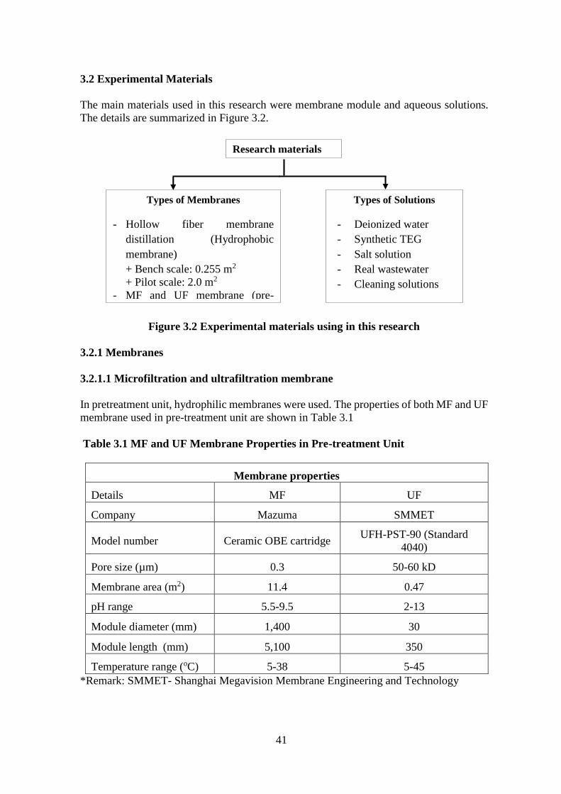
41
3.2 Experimental Materials
The main materials used in this research were membrane module and aqueous solutions.
The details are summarized in Figure 3.2.
Figure 3.2 Experimental materials using in this research
3.2.1 Membranes
3.2.1.1 Microfiltration and ultrafiltration membrane
In pretreatment unit, hydrophilic membranes were used. The properties of both MF and UF
membrane used in pre-treatment unit are shown in Table 3.1
Table 3.1 MF and UF Membrane Properties in Pre-treatment Unit
Membrane properties
Details MF UF
Company Mazuma SMMET
Model number Ceramic OBE cartridge UFH-PST-90 (Standard
4040)
Pore size (µm) 0.3 50-60 kD
Membrane area (m2) 11.4 0.47
pH range 5.5-9.5 2-13
Module diameter (mm) 1,400 30
Module length (mm) 5,100 350
Temperature range (oC) 5-38 5-45
*Remark: SMMET- Shanghai Megavision Membrane Engineering and Technology
Research materials
Types of Membranes
- Hollow fiber membrane
distillation (Hydrophobic
membrane)
+ Bench scale: 0.255 m2
+ Pilot scale: 2.0 m2
- MF and UF membrane (pre-
Types of Solutions
- Deionized water
- Synthetic TEG
- Salt solution
- Real wastewater
- Cleaning solutions

42
3.2.1.2 Membrane distillation
The characteristics of membrane used in bench scale and pilot scale unit are shown in Table
3.2. The fabrication of hollow fiber membrane aims to achieve high packing density
(m2/m3). It was difficult to clean the membrane module in this fabrication. Thus, the
pretreatment system was required to work well generating very less solid particles in the
effluent source. In this study, feed solution was fed at outer surface of fiber while sweeping
gas would go into the inner side of fiber (outside-in configuration). The hydrophobic nature
of this membrane avoided liquid to enter the membrane pore.
Table 3.2 Hollow Fiber Membrane Distillation Specification
Descriptions Characteristics
Bench scale unit Pilot scale unit
Company Name Sumitomo Electric Industries, Ltd.
Membrane Name TB-21-02 PM-X215
Type No. 130529-1 13001-2
Module Configuration Hollow Fiber
Membrane Material Polytetrafluoethylene (PTFE)
Type of Membrane Hydrophobic microporous
Contact Angle 112o
Nominal Pore Size (μm) 0.45
Outside Diameter (mm) 2.03
Inside Diameter (mm) 1.07
Total Length (mm) 500 1105
Effective Length (mm) 400 1008
Thickness (μm) 480
Number of fibers 100 306
Membrane Effective Area (m2) 0.255 2
Operating Temperature Range (oC) -100 to 260
pH Range 0-14
Hollow fiber membrane distillation module
The specification of hollow fiber membrane module ws summarized in Table 3.3.
3.2.2 Experimental solutions
3.2.2.1 Deionized water
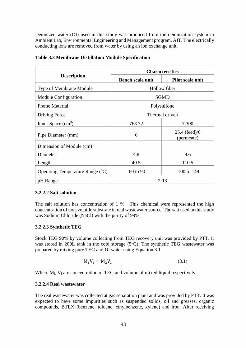
43
Deionized water (DI) used in this study was produced from the deionization system in
Ambient Lab, Environmental Engineering and Management program, AIT. The electrically
conducting ions are removed from water by using an ion exchange unit.
Table 3.3 Membrane Distillation Module Specification
Description Characteristics
Bench scale unit Pilot scale unit
Type of Membrane Module Hollow fiber
Module Configuration SGMD
Frame Material Polysulfone
Driving Force Thermal driven
Inner Space (cm3) 763.72 7,300
Pipe Diameter (mm) 6 25.4 (feed)/6
(permeate)
Dimension of Module (cm)
Diameter
Length
4.8
40.5
9.6
110.5
Operating Temperature Range (oC) -60 to 90 -100 to 149
pH Range 2-13
3.2.2.2 Salt solution
The salt solution has concentration of 1 %. This chemical were represented the high
concentration of non-volatile substrate in real wastewater source. The salt used in this study
was Sodium Chloride (NaCl) with the purity of 99%.
3.2.2.3 Synthetic TEG
Stock TEG 90% by volume collecting from TEG recovery unit was provided by PTT. It
was stored in 200L tank in the cold storage (5oC). The synthetic TEG wastewater was
prepared by mixing pure TEG and DI water using Equation 3.1.
M1V1 = M2V2 (3.1)
Where Mi, Vi are concentration of TEG and volume of mixed liquid respectively
3.2.2.4 Real wastewater
The real wastewater was collected at gas separation plant and was provided by PTT. It was
expected to have some impurities such as suspended solids, oil and greases, organic
compounds, BTEX (benzene, toluene, ethylbenzene, xylene) and iron. After receiving

44
wastewater from PTT, it was stored in a composite container and was pre-treated before
operating with MD system.
3.2.2.5 Cleaning chemicals
Chemical agents which were used to clean the hydrophobic membrane were a mixture of
oxalic and citric acid. This cleaning solution had been proven as an efficient solution to
clean the hydrophobic membrane distillation (Guillen-Burrieza et al., 2014). The specific
information of the cleaning chemicals are described in Table 3.4.
Table 3.4 Cleaning Chemicals Used in this Study
Generic
Name
Chemical
Formula
MW
(g/mol) CAS No.
Purity
(%) Supplier
Citric Acid C6H8O7 192.12 77-92-9 99.8
U & V Holding Co., Ltd Oxalic
Acid C2H2O4 90.03 144-62-7 99.8
3.3 Experimental Methods
3.3.1 Experimental set-up
Pre-treatment unit
The pre-treatment unit was a combined membrane system, hollow fiber ultrafiltration
membrane (UF) followed by cartridge microfiltration membrane (MF). This unit played
as a physical filtration barrier, to remove suspended solids (by MF), oil and grease (by UF).
By removing of such impurities, pre-treatment unit helped to minimize the particle fouling
phenomena and increase the separating efficiency of MD module. The schematic diagram
of pre-treatment unit is clearly described in Figure 3.3.
In the raw wastewater tank, an air diffuser was installed. The purpose of adding air diffuser
was to remove BTEX and transfer iron ion to ferric hydroxide (Fe(OH)3). The air-to-water
ratio was based on the concentration of iron in wastewater. Beside, viscosity of raw
wastewater also reduced slightly after passing through pretreatment unit. It would lead to
reduce fouling condition.
The parameters which were used to evaluate pre-treatment unit’s performance are:
turbidity, oil and grease, BTEX, TEG concentration, and fouling
Bench scale system set-up
Crossing flow mode was used as the mode operation of this study. Feed aqueous solution
contacted directly and was circulated in cross flow mode over the feed surface of
membrane. Sweep gas contacted the membrane surface and crossed the permeate side. Heat
and mass transfer would cross the hydrophobic porous structure of membrane. It led to
reduce effect of boundary layer resistance. Moreover, the effect of concentration and
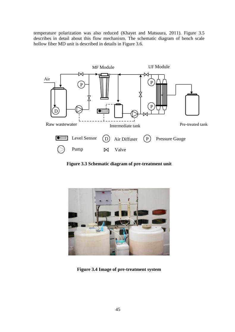
45
temperature polarization was also reduced (Khayet and Matsuura, 2011). Figure 3.5
describes in detail about this flow mechanism. The schematic diagram of bench scale
hollow fiber MD unit is described in details in Figure 3.6.
Figure 3.3 Schematic diagram of pre-treatment unit
Figure 3.4 Image of pre-treatment system
Raw wastewater tank
D
Intermediate tank Pre-treated tank
UF Module MF Module
P
Air
P P
Level Sensor D Air Diffuser P Pressure Gauge
Pump Valve
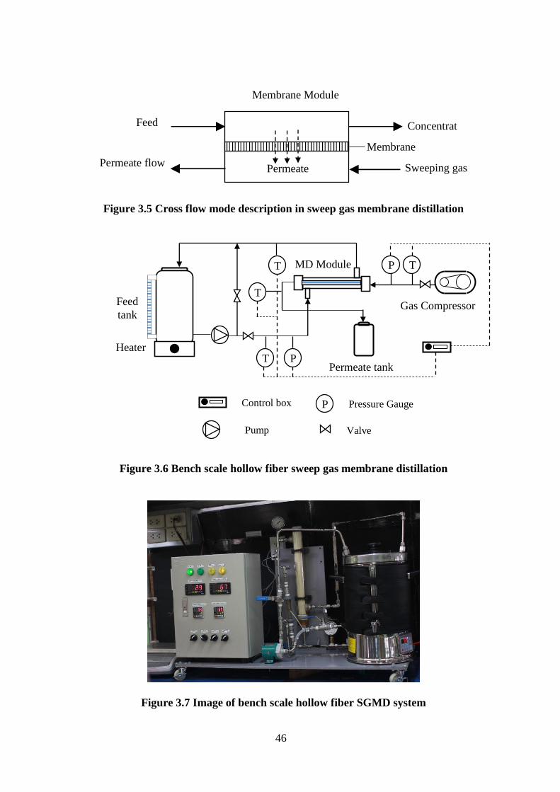
46
Figure 3.5 Cross flow mode description in sweep gas membrane distillation
Figure 3.6 Bench scale hollow fiber sweep gas membrane distillation
Figure 3.7 Image of bench scale hollow fiber SGMD system
Membrane
Permeate
Feed
Sweeping gas
Concentrat
e
Membrane Module
Permeate flow
Control box P Pressure Gauge
Pump Valve
Permeate tank
T
T
P T Heater
Feed
tank
T P
Gas Compressor
MD Module
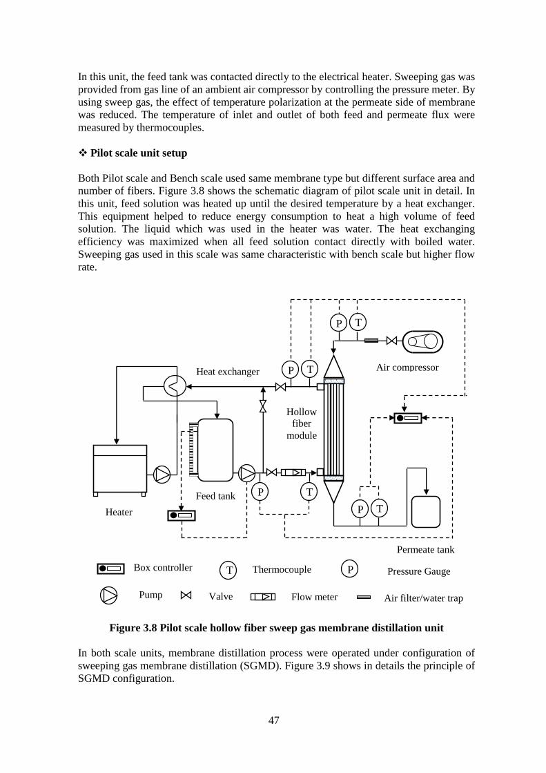
47
In this unit, the feed tank was contacted directly to the electrical heater. Sweeping gas was
provided from gas line of an ambient air compressor by controlling the pressure meter. By
using sweep gas, the effect of temperature polarization at the permeate side of membrane
was reduced. The temperature of inlet and outlet of both feed and permeate flux were
measured by thermocouples.
Pilot scale unit setup
Both Pilot scale and Bench scale used same membrane type but different surface area and
number of fibers. Figure 3.8 shows the schematic diagram of pilot scale unit in detail. In
this unit, feed solution was heated up until the desired temperature by a heat exchanger.
This equipment helped to reduce energy consumption to heat a high volume of feed
solution. The liquid which was used in the heater was water. The heat exchanging
efficiency was maximized when all feed solution contact directly with boiled water.
Sweeping gas used in this scale was same characteristic with bench scale but higher flow
rate.
Figure 3.8 Pilot scale hollow fiber sweep gas membrane distillation unit
In both scale units, membrane distillation process were operated under configuration of
sweeping gas membrane distillation (SGMD). Figure 3.9 shows in details the principle of
SGMD configuration.
Heat exchanger
Heater
Feed tank
Permeate tank
Air compressor
Hollow
fiber
module
P T
P T
T
P T
P
Box controller T Thermocouple P Pressure Gauge
Pump Valve Flow meter Air filter/water trap
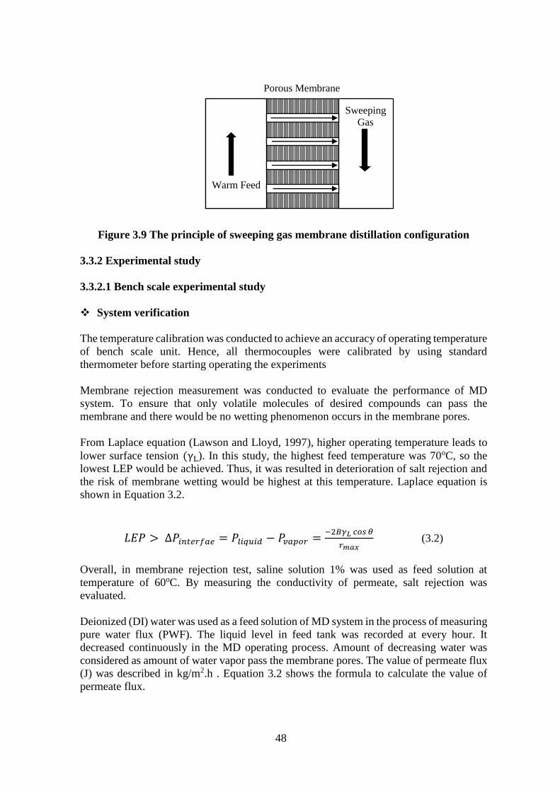
48
Figure 3.9 The principle of sweeping gas membrane distillation configuration
3.3.2 Experimental study
3.3.2.1 Bench scale experimental study
System verification
The temperature calibration was conducted to achieve an accuracy of operating temperature
of bench scale unit. Hence, all thermocouples were calibrated by using standard
thermometer before starting operating the experiments
Membrane rejection measurement was conducted to evaluate the performance of MD
system. To ensure that only volatile molecules of desired compounds can pass the
membrane and there would be no wetting phenomenon occurs in the membrane pores.
From Laplace equation (Lawson and Lloyd, 1997), higher operating temperature leads to
lower surface tension (γL). In this study, the highest feed temperature was 70oC, so the
lowest LEP would be achieved. Thus, it was resulted in deterioration of salt rejection and
the risk of membrane wetting would be highest at this temperature. Laplace equation is
shown in Equation 3.2.
𝐿𝐸𝑃 > ∆𝑃𝑖𝑛𝑡𝑒𝑟𝑓𝑎𝑒 = 𝑃𝑙𝑖𝑞𝑢𝑖𝑑 − 𝑃𝑣𝑎𝑝𝑜𝑟 =−2𝐵𝛾𝐿 𝑐𝑜𝑠 𝜃
𝑟𝑚𝑎𝑥 (3.2)
Overall, in membrane rejection test, saline solution 1% was used as feed solution at
temperature of 60oC. By measuring the conductivity of permeate, salt rejection was
evaluated.
Deionized (DI) water was used as a feed solution of MD system in the process of measuring
pure water flux (PWF). The liquid level in feed tank was recorded at every hour. It
decreased continuously in the MD operating process. Amount of decreasing water was
considered as amount of water vapor pass the membrane pores. The value of permeate flux
(J) was described in kg/m2.h . Equation 3.2 shows the formula to calculate the value of
permeate flux.
Warm Feed
Sweeping
Gas
Porous Membrane
49
𝐽 =𝑉𝑗−𝑉𝑖
𝐴×𝑡 (3.3)
Where V𝑖 , Vj, A, t are the volume of solution in feed tank at time i and j, membrane surface
area and time of measuring respectively.
From PWF, membrane coefficient (Bw) and membrane resistance (Rm) was calculated by
using Equation 3.4. Rm was the resistance of a membrane when it was still not yet affected
by other resistances (i.e. boundary layer resistance). Rm of pure feed water was used to
compare with other feed solution to evaluate fouling condition.
𝐽 = 𝐵𝑤 × ∆𝑝𝑊 = 1
𝑅𝑚× ∆𝑝𝑊 (3.4)
Temperatures of feed pure water were 50, 60 and 70oC, feed flow rates were 1.8, 2 and 2.4
L/min. At the permeate side, the sweeping gas flow rate was depended on the pressure, it
could be high as possible if there was no undesirable pressure developed. The operation
period of each batch was 8 hours and data collection was conducted at every hour.
Synthetic TEG wastewater test
Before testing with real TEG wastewater, bench scale hollow fiber SGMD unit was tested
with synthetic wastewater first. From synthetic wastewater study, the optimum TEG
concentration was found out without affecting of any other impurities in feed solution.
There were 7 levels of initial TEG concentration, obtains 5, 10, 20, 30, 40, 50, 60 %.
At each initial TEG concentration, the experiment was run totally 8 hours. The intention
of choosing 8 hours was to evaluate the system’s performance within time of official
working day. The permeate flux was measure at every hour of this 8 hours. For TEG
sample, there were two different samples: initial concentration sample and the sample of
TEG solution after 8 hours of operating.
Real TEG wastewater test
After testing with synthetic wastewater, the bench scale MD unit was test with real
wastewater. There are many other impurities in real wastewater, especially suspended
solids, oil and grease, BTEX. These impurities would increase the opportunity of
membrane fouling. A MF combined with UF system was the appropriate pre-treatment
system for this wastewater. The TEG concentration in real wastewater, in fact, was various
from 5 to 20%, it was uncontrollable. All the measurements of real wastewater testing were
same with synthetic wastewater testing.
3.3.2.2 Pilot scale experimental study
The optimum operating condition was chosen from bench scale hollow fiber SGMD study
(base on permeate flux, TEG concentrating ability, and energy consumption). In the second
phase of this study, the optimum condition from first phase study was applied to operate
the pilot scale hollow fiber SGMD unit. From the experimental results, a full scale SGMD
plant was designed and was accepted by the gas separation plant.
50
System verification
In this phase, only feed temperature at the best- performance condition from bench scale
study was used to operate the pilot scale unit. The feed flow rate, and sweeping gas flow
rate were changed to adapt with a larger scale in comparison with the dimension of bench
scale hollow fiber module and membrane area.
From pure water flux, the coefficient of membrane distillation (Bw) and membrane
resistance (Rm) in pilot scale were calculated. These values present the properties of
membrane in pilot scale and was used for further study on membrane fouling phenomenon.
In the rejection test of pilot scale, due to the reaction between salt (NaCl) and copper (Cu)
in the heat exchanger, TEG solution (10%) was selected. By measuring the TEG
concentration (TEG played as non-volatile compound) at both feed solution and permeate
condense, the rejection ability of membrane was calculated. The evaluation on rejecting of
undesirable compound was a need for every membrane distillation experiment. The pilot
system must be ensured that the pores do not get wetting and only desired compound can
pass the hydrophobic porous membrane. According to Equation 3.2, 70oC was the feed
temperature used in rejection test.
Synthetic TEG wastewater test
The concentration of synthetic TEG wastewater was used in pilot scale unit was the TEG
concentration used in bench scale unit study. Equation 3.1 was used to prepare this
concentration of synthetic TEG wastewater. Permeate flux and energy consumption were
measured at every hour of 8 hours experiment. Membrane fouling phenomena was
evaluated from the value of membrane coefficient in this experiment.
Real TEG wastewater test
Similar with real TEG wastewater test in bench scale unit, pilot scale SGMD was also
tested with real wastewater. The reason for testing with real wastewater was due to the
reality that wastewater contains impurities and uncontrollable concentration. Real
wastewater was stored in a feed tank of 52 L and supplied continuously to the hollow fiber
module for whole 8 hours of experiment. The sample of real wastewater was taken at three
points of timeline: before pre-treatment unit, before operating the pilot scale unit, and every
8 hours of operation. Both real wastewater and Synthetic TEG experiments were test with
two operating method: batch experiment (8 hours per batch) and continuously-fed
experiment (40 hours, equal to 5 working days per week)
3.3.3 Energy consumption evaluation
Energy consumption by MD system was measured by the power meters. At each scenario
of operation, the value of ratio between energy consumption and permeate flow rate would
be considered. The lowest value means highest energy efficiency. The ratio between
energy consumption and permeate flow rate were described in a unit of (kW/kg.h) by using
Equation 3.5.
E =∑ Power consumed (kW)
Permeate flux (kg m2⁄ h)×Membrane area (m2) (3.5)
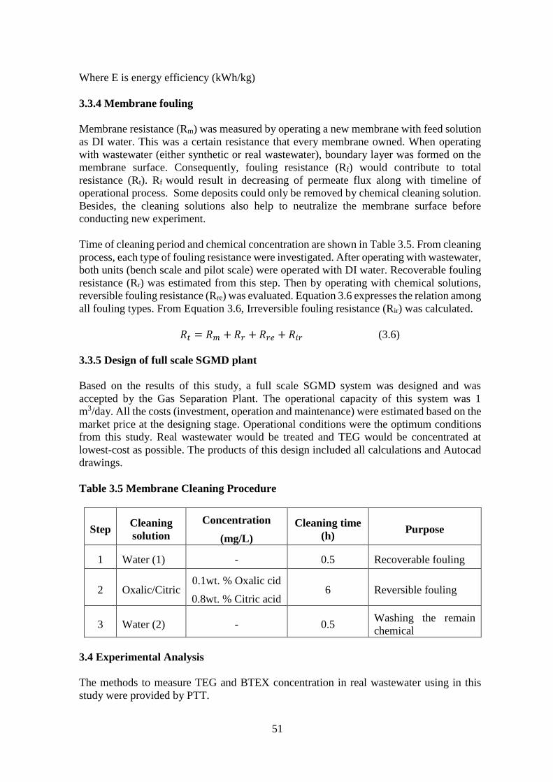
51
Where E is energy efficiency (kWh/kg)
3.3.4 Membrane fouling
Membrane resistance (Rm) was measured by operating a new membrane with feed solution
as DI water. This was a certain resistance that every membrane owned. When operating
with wastewater (either synthetic or real wastewater), boundary layer was formed on the
membrane surface. Consequently, fouling resistance (Rf) would contribute to total
resistance (Rt). Rf would result in decreasing of permeate flux along with timeline of
operational process. Some deposits could only be removed by chemical cleaning solution.
Besides, the cleaning solutions also help to neutralize the membrane surface before
conducting new experiment.
Time of cleaning period and chemical concentration are shown in Table 3.5. From cleaning
process, each type of fouling resistance were investigated. After operating with wastewater,
both units (bench scale and pilot scale) were operated with DI water. Recoverable fouling
resistance (Rr) was estimated from this step. Then by operating with chemical solutions,
reversible fouling resistance (Rre) was evaluated. Equation 3.6 expresses the relation among
all fouling types. From Equation 3.6, Irreversible fouling resistance (Rir) was calculated.
𝑅𝑡 = 𝑅𝑚 + 𝑅𝑟 + 𝑅𝑟𝑒 + 𝑅𝑖𝑟 (3.6)
3.3.5 Design of full scale SGMD plant
Based on the results of this study, a full scale SGMD system was designed and was
accepted by the Gas Separation Plant. The operational capacity of this system was 1
m3/day. All the costs (investment, operation and maintenance) were estimated based on the
market price at the designing stage. Operational conditions were the optimum conditions
from this study. Real wastewater would be treated and TEG would be concentrated at
lowest-cost as possible. The products of this design included all calculations and Autocad
drawings.
Table 3.5 Membrane Cleaning Procedure
Step Cleaning
solution
Concentration
(mg/L)
Cleaning time
(h) Purpose
1 Water (1) - 0.5 Recoverable fouling
2 Oxalic/Citric 0.1wt. % Oxalic cid
0.8wt. % Citric acid 6 Reversible fouling
3 Water (2) - 0.5 Washing the remain
chemical
3.4 Experimental Analysis
The methods to measure TEG and BTEX concentration in real wastewater using in this
study were provided by PTT.
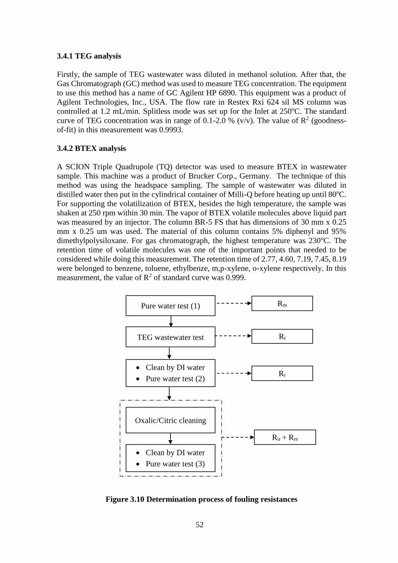
52
3.4.1 TEG analysis
Firstly, the sample of TEG wastewater wass diluted in methanol solution. After that, the
Gas Chromatograph (GC) method was used to measure TEG concentration. The equipment
to use this method has a name of GC Agilent HP 6890. This equipment was a product of
Agilent Technologies, Inc., USA. The flow rate in Restex Rxi 624 sil MS column was
controlled at 1.2 mL/min. Splitless mode was set up for the Inlet at 250oC. The standard
curve of TEG concentration was in range of 0.1-2.0 % (v/v). The value of R2 (goodness-
of-fit) in this measurement was 0.9993.
3.4.2 BTEX analysis
A SCION Triple Quadrupole (TQ) detector was used to measure BTEX in wastewater
sample. This machine was a product of Brucker Corp., Germany. The technique of this
method was using the headspace sampling. The sample of wastewater was diluted in
distilled water then put in the cylindrical container of Milli-Q before heating up until 80oC.
For supporting the volatilization of BTEX, besides the high temperature, the sample was
shaken at 250 rpm within 30 min. The vapor of BTEX volatile molecules above liquid part
was measured by an injector. The column BR-5 FS that has dimensions of 30 mm x 0.25
mm x 0.25 um was used. The material of this column contains 5% diphenyl and 95%
dimethylpolysiloxane. For gas chromatograph, the highest temperature was 230oC. The
retention time of volatile molecules was one of the important points that needed to be
considered while doing this measurement. The retention time of 2.77, 4.60, 7.19, 7.45, 8.19
were belonged to benzene, toluene, ethylbenze, m,p-xylene, o-xylene respectively. In this
measurement, the value of R2 of standard curve was 0.999.
Figure 3.10 Determination process of fouling resistances
Pure water test (1)
TEG wastewater test
Oxalic/Citric cleaning
Rm
Rt
Rr
Rir + Rre
Clean by DI water
Pure water test (3)
Clean by DI water
Pure water test (2)
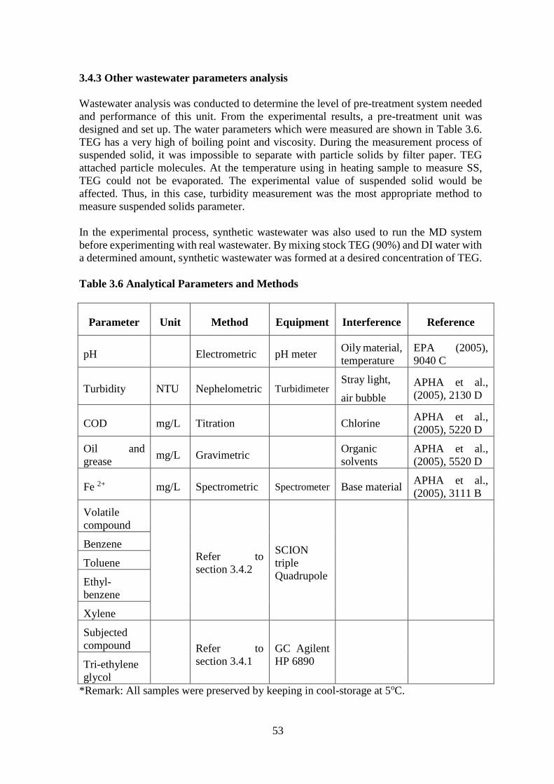
53
3.4.3 Other wastewater parameters analysis
Wastewater analysis was conducted to determine the level of pre-treatment system needed
and performance of this unit. From the experimental results, a pre-treatment unit was
designed and set up. The water parameters which were measured are shown in Table 3.6.
TEG has a very high of boiling point and viscosity. During the measurement process of
suspended solid, it was impossible to separate with particle solids by filter paper. TEG
attached particle molecules. At the temperature using in heating sample to measure SS,
TEG could not be evaporated. The experimental value of suspended solid would be
affected. Thus, in this case, turbidity measurement was the most appropriate method to
measure suspended solids parameter.
In the experimental process, synthetic wastewater was also used to run the MD system
before experimenting with real wastewater. By mixing stock TEG (90%) and DI water with
a determined amount, synthetic wastewater was formed at a desired concentration of TEG.
Table 3.6 Analytical Parameters and Methods
Parameter Unit Method Equipment Interference Reference
pH Electrometric pH meter Oily material,
temperature
EPA (2005),
9040 C
Turbidity NTU Nephelometric Turbidimeter Stray light,
air bubble
APHA et al.,
(2005), 2130 D
COD mg/L Titration Chlorine APHA et al.,
(2005), 5220 D
Oil and
grease mg/L Gravimetric
Organic
solvents
APHA et al.,
(2005), 5520 D
Fe 2+ mg/L Spectrometric Spectrometer Base material APHA et al.,
(2005), 3111 B
Volatile
compound
Refer to
section 3.4.2
SCION
triple
Quadrupole
Benzene
Toluene
Ethyl-
benzene
Xylene
Subjected
compound
Refer to
section 3.4.1
GC Agilent
HP 6890
Tri-ethylene
glycol
*Remark: All samples were preserved by keeping in cool-storage at 5oC.
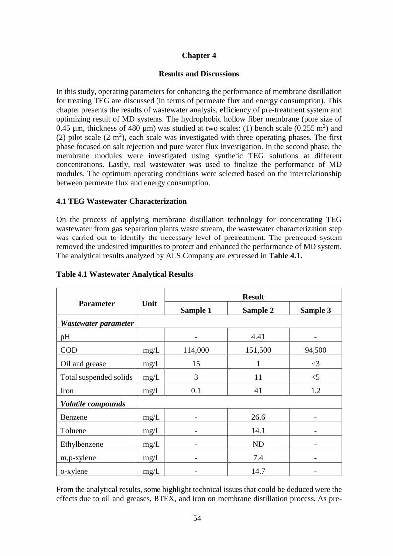
54
Chapter 4
Results and Discussions
In this study, operating parameters for enhancing the performance of membrane distillation
for treating TEG are discussed (in terms of permeate flux and energy consumption). This
chapter presents the results of wastewater analysis, efficiency of pre-treatment system and
optimizing result of MD systems. The hydrophobic hollow fiber membrane (pore size of
0.45 µm, thickness of 480 µm) was studied at two scales: (1) bench scale (0.255 m2) and
(2) pilot scale (2 m2), each scale was investigated with three operating phases. The first
phase focused on salt rejection and pure water flux investigation. In the second phase, the
membrane modules were investigated using synthetic TEG solutions at different
concentrations. Lastly, real wastewater was used to finalize the performance of MD
modules. The optimum operating conditions were selected based on the interrelationship
between permeate flux and energy consumption.
4.1 TEG Wastewater Characterization
On the process of applying membrane distillation technology for concentrating TEG
wastewater from gas separation plants waste stream, the wastewater characterization step
was carried out to identify the necessary level of pretreatment. The pretreated system
removed the undesired impurities to protect and enhanced the performance of MD system.
The analytical results analyzed by ALS Company are expressed in Table 4.1.
Table 4.1 Wastewater Analytical Results
Parameter Unit Result
Sample 1 Sample 2 Sample 3
Wastewater parameter
pH - 4.41 -
COD mg/L 114,000 151,500 94,500
Oil and grease mg/L 15 1 <3
Total suspended solids mg/L 3 11 <5
Iron mg/L 0.1 41 1.2
Volatile compounds
Benzene mg/L - 26.6 -
Toluene mg/L - 14.1 -
Ethylbenzene mg/L - ND -
m,p-xylene mg/L - 7.4 -
o-xylene mg/L - 14.7 -
From the analytical results, some highlight technical issues that could be deduced were the
effects due to oil and greases, BTEX, and iron on membrane distillation process. As pre-

55
treatment, total suspended solids (TSS) and oil and grease (O&G) had to be removed and
be eliminated since they could foul the membrane surface (and/or membrane module). The
concentration of iron as is observed in sample 2 (41 mg/L) was another problem. During
concentrating TEG wastewater, the solubility limit of iron in the concentrated solution
would be reached and iron could potentially precipitated on the membrane surface.
However in sample 1, 2 and 3, high iron concentration was not always observed (0.1 mg/L
in sample 1 and 1.2 mg/L in sample 2). This fluctuation could have occurred due to a
process instability at the methane production site at the GSP. Another observed issue is that
the appearance of volatile compounds in wastewater. Volatile compounds such as benzene,
toluene, ethyl benzene and xylene (BTEX) were found in the wastewater (Table 4.1),
which were also categorised as carcinogen compounds. During operating MD process, such
compounds would pass through the membrane pores and could reduce the hydrophobicity
of the membrane and also cause health effects to the operators. Practically, by providing
aeration into the wastewater prior pre-treatment unit, BTEX could be vaporized due to high
volatility and iron could be precipitated through oxidation reaction. Oil and grease are the
organic species which contains hydrophobic components in the molecule structure. This
such molecules can readily attach onto the membrane surface and lead to process failure in
MD. This could lead to the formation of hydrophilic tracks through the pores. This
approach allows water to (a polar specie) interact with the hydrophilic section of oil and
grease. Thus, it would be a potential risk of liquid penetration into the pores (Padaki et al.,
2015). Overall, it was necessary to install a pre-treatment system prior MD unit. A proper
pre-treated wastewater could lead to an effective performance of MD process for long term
operation.
4.2 Performance of Pre-treatment Unit
As presented in Section 4.1, the pre-treatment system was installed to eliminate suspended
solids, oil and grease predominantly. Such undesired impurities might cause membrane
fouling issues and affect the hydrophobic characteristic. The performance of the process
was determined by comparing the quality parameters such as: raw wastewater (before pre-
treatment unit), effluent from microfiltration membrane (MF), and pre-treated wastewater
(after passing through ultrafiltration – UF). The measured parameters and analytical results
are shown in Table 4.2
Table 4.2 Analytical Results of Pre-treating Samples
Parameters Raw Wastewater After MF After UF
COD (g/L) 151.5 157.9 150.50
Turbidity (NTU) 30.69 4.21 1.27
Suspended solids (mg/L) 11 <5 <5
pH 4.41 4.48 4.46
O&G (mg/L) 15.00 7.00 5.00
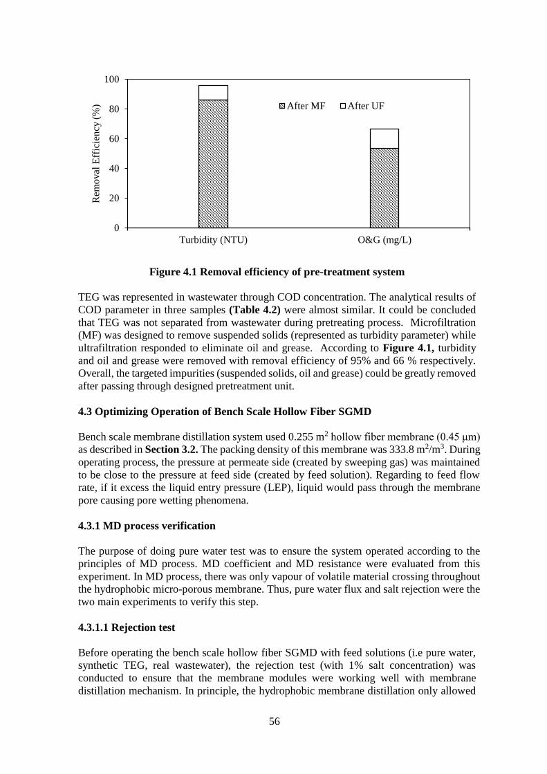
56
Figure 4.1 Removal efficiency of pre-treatment system
TEG was represented in wastewater through COD concentration. The analytical results of
COD parameter in three samples (Table 4.2) were almost similar. It could be concluded
that TEG was not separated from wastewater during pretreating process. Microfiltration
(MF) was designed to remove suspended solids (represented as turbidity parameter) while
ultrafiltration responded to eliminate oil and grease. According to Figure 4.1, turbidity
and oil and grease were removed with removal efficiency of 95% and 66 % respectively.
Overall, the targeted impurities (suspended solids, oil and grease) could be greatly removed
after passing through designed pretreatment unit.
4.3 Optimizing Operation of Bench Scale Hollow Fiber SGMD
Bench scale membrane distillation system used 0.255 m2 hollow fiber membrane (0.45 μm)
as described in Section 3.2. The packing density of this membrane was 333.8 m2/m3. During
operating process, the pressure at permeate side (created by sweeping gas) was maintained
to be close to the pressure at feed side (created by feed solution). Regarding to feed flow
rate, if it excess the liquid entry pressure (LEP), liquid would pass through the membrane
pore causing pore wetting phenomena.
4.3.1 MD process verification
The purpose of doing pure water test was to ensure the system operated according to the
principles of MD process. MD coefficient and MD resistance were evaluated from this
experiment. In MD process, there was only vapour of volatile material crossing throughout
the hydrophobic micro-porous membrane. Thus, pure water flux and salt rejection were the
two main experiments to verify this step.
4.3.1.1 Rejection test
Before operating the bench scale hollow fiber SGMD with feed solutions (i.e pure water,
synthetic TEG, real wastewater), the rejection test (with 1% salt concentration) was
conducted to ensure that the membrane modules were working well with membrane
distillation mechanism. In principle, the hydrophobic membrane distillation only allowed
0
20
40
60
80
100
Turbidity (NTU) O&G (mg/L)
Rem
oval
Eff
icie
ncy
(%
) After MF After UF
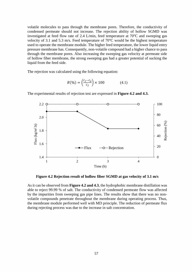
57
volatile molecules to pass through the membrane pores. Therefore, the conductivity of
condensed permeate should not increase. The rejection ability of hollow SGMD was
investigated at feed flow rate of 2.4 L/min, feed temperature at 70oC and sweeping gas
velocity of 3.1 and 5.3 m/s. Feed temperature of 70oC would be the highest temperature
used to operate the membrane module. The higher feed temperature, the lower liquid entry
pressure membrane has. Consequently, non-volatile compound had a higher chance to pass
through the membrane pores. Also increasing the sweeping gas velocity at permeate side
of hollow fiber membrane, the strong sweeping gas had a greater potential of sucking the
liquid from the feed side.
The rejection was calculated using the following equation:
𝑅(%) = (𝐶𝑓−𝐶𝑝
𝐶𝑓) × 100 (4.1)
The experimental results of rejection test are expressed in Figure 4.2 and 4.3.
Figure 4.2 Rejection result of hollow fiber SGMD at gas velocity of 3.1 m/s
As it can be observed from Figure 4.2 and 4.3, the hydrophobic membrane distillation was
able to reject 99.99 % of salt. The conductivity of condensed permeate flow was affected
by the impurities from sweeping gas pipe lines. The results show that there was no non-
volatile compounds penetrate throughout the membrane during operating process. Thus,
the membrane module performed well with MD principle. The reduction of permeate flux
during rejecting process was due to the increase in salt concentration.
0
20
40
60
80
100
1.4
1.6
1.8
2.0
2.2
1 2 3 4R
ejec
tion (
%)
Flu
x (
kg/m
2.h
)
Time (h)
Flux Rejection

58
Figure 4.3 Rejection result of hollow fiber SGMD at gas velocity of 5.3 m/s
4.3.1.2 Pure water test
Hollow fiber membrane module was investigated with DI water. The experimental variables
in bench scale study were feed flow rate at 1.8, 2, 2.4 L/min, feed temperature at 50, 60,
70oC, sweeping gas velocity at 3.1, 3.6, 4.2, 4.7, 5.3 m/s. The driving force in MD process
is the difference in vapour pressure between feed side (liquid phase) and permeate side (gas
phase) of the fiber. Increasing feed temperature, the vapour pressure of water also increases.
Vapour pressure strongly affected by the feed temperature. At the same feed flow rate, same
sweeping gas velocity but lower feed temperature, the permeate flux was lower
significantly. When increasing the sweeping gas velocity, permeate flux also corresponding
increases too. However, as the vapour pressure increases at permeate side this leads to a
decrease in the driving force of MD process. When the sweeping gas velocity exceed a
certain value, the pressure at permeate side is higher than feed side. At this situation, some
air bubble started to appear at the feed side of the membrane.
Effect of feed inlet flow rate
Figure 4.4 presents the effects of various feed inlet flow rates on permeate flux at different
sweeping gas inlet velocities and feed temperature of 70oC. At the same operating conditions
(gas velocity, feed flow rate, feed temperature), the achieved permeate flux were almost
similar. The small difference of permeate fluxes at the sweeping gas velocity were due to
the slightly reduction of boundary layer resistance at the feed membrane surface.
0
20
40
60
80
100
2.0
2.3
2.6
2.9
3.2
1 2 3 4
Rej
ecti
on
(%
)
Flu
x (
kg/m
2.h
)
Time (h)
Flux Rejection
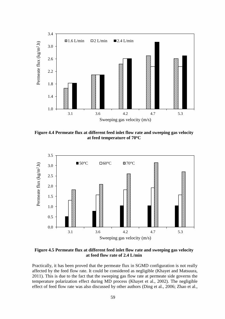
59
Figure 4.4 Permeate flux at different feed inlet flow rate and sweeping gas velocity
at feed temperature of 70oC
Figure 4.5 Permeate flux at different feed inlet flow rate and sweeping gas velocity
at feed flow rate of 2.4 L/min
Practically, it has been proved that the permeate flux in SGMD configuration is not really
affected by the feed flow rate. It could be considered as negligible (Khayet and Matsuura,
2011). This is due to the fact that the sweeping gas flow rate at permeate side governs the
temperature polarization effect during MD process (Khayet et al., 2002). The negligible
effect of feed flow rate was also discussed by other authors (Ding et al., 2006; Zhao et al.,
1.0
1.4
1.8
2.2
2.6
3.0
3.4
3.1 3.6 4.2 4.7 5.3
Per
mea
te f
lux
(kg/m
2.h
)
Sweeping gas velocity (m/s)
1.6 L/min 2 L/min 2.4 L/min
0.0
0.5
1.0
1.5
2.0
2.5
3.0
3.5
3.1 3.6 4.2 4.7 5.3
Per
mea
te f
lux
(kg/m
2.h
)
Sweeping gas velocity (m/s)
50°C 60°C 70°C
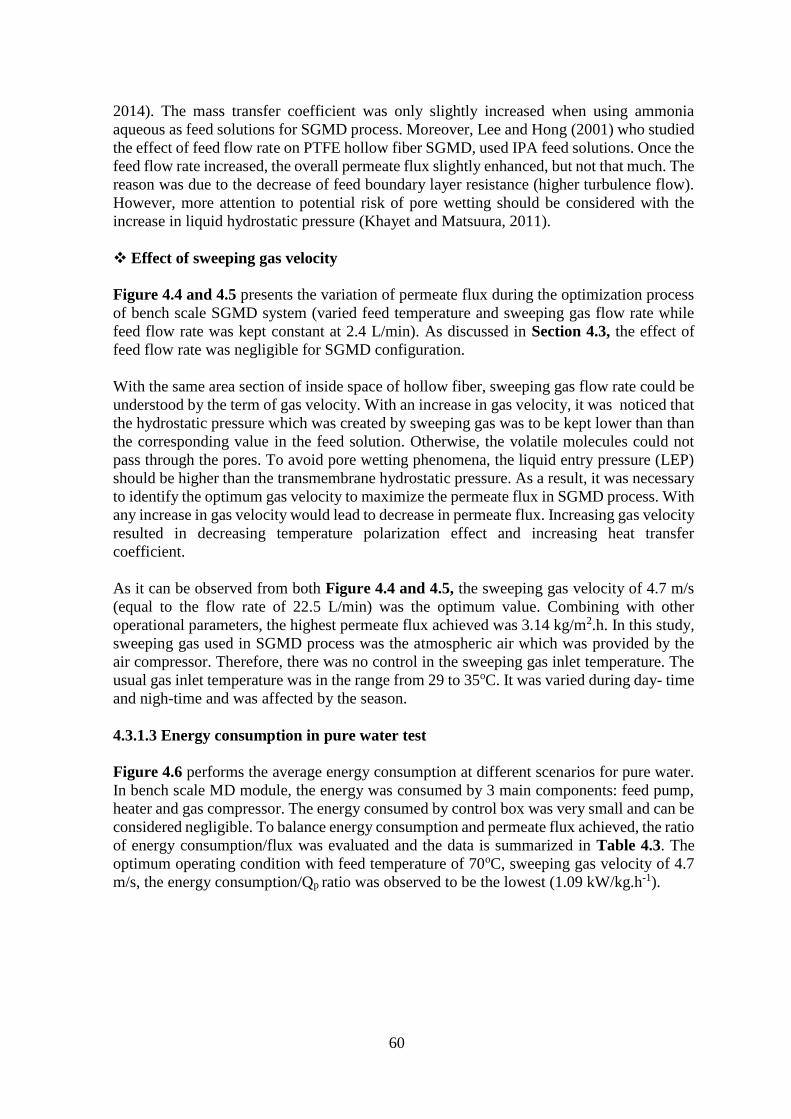
60
2014). The mass transfer coefficient was only slightly increased when using ammonia
aqueous as feed solutions for SGMD process. Moreover, Lee and Hong (2001) who studied
the effect of feed flow rate on PTFE hollow fiber SGMD, used IPA feed solutions. Once the
feed flow rate increased, the overall permeate flux slightly enhanced, but not that much. The
reason was due to the decrease of feed boundary layer resistance (higher turbulence flow).
However, more attention to potential risk of pore wetting should be considered with the
increase in liquid hydrostatic pressure (Khayet and Matsuura, 2011).
Effect of sweeping gas velocity
Figure 4.4 and 4.5 presents the variation of permeate flux during the optimization process
of bench scale SGMD system (varied feed temperature and sweeping gas flow rate while
feed flow rate was kept constant at 2.4 L/min). As discussed in Section 4.3, the effect of
feed flow rate was negligible for SGMD configuration.
With the same area section of inside space of hollow fiber, sweeping gas flow rate could be
understood by the term of gas velocity. With an increase in gas velocity, it was noticed that
the hydrostatic pressure which was created by sweeping gas was to be kept lower than than
the corresponding value in the feed solution. Otherwise, the volatile molecules could not
pass through the pores. To avoid pore wetting phenomena, the liquid entry pressure (LEP)
should be higher than the transmembrane hydrostatic pressure. As a result, it was necessary
to identify the optimum gas velocity to maximize the permeate flux in SGMD process. With
any increase in gas velocity would lead to decrease in permeate flux. Increasing gas velocity
resulted in decreasing temperature polarization effect and increasing heat transfer
coefficient.
As it can be observed from both Figure 4.4 and 4.5, the sweeping gas velocity of 4.7 m/s
(equal to the flow rate of 22.5 L/min) was the optimum value. Combining with other
operational parameters, the highest permeate flux achieved was 3.14 kg/m2.h. In this study,
sweeping gas used in SGMD process was the atmospheric air which was provided by the
air compressor. Therefore, there was no control in the sweeping gas inlet temperature. The
usual gas inlet temperature was in the range from 29 to 35oC. It was varied during day- time
and nigh-time and was affected by the season.
4.3.1.3 Energy consumption in pure water test
Figure 4.6 performs the average energy consumption at different scenarios for pure water.
In bench scale MD module, the energy was consumed by 3 main components: feed pump,
heater and gas compressor. The energy consumed by control box was very small and can be
considered negligible. To balance energy consumption and permeate flux achieved, the ratio
of energy consumption/flux was evaluated and the data is summarized in Table 4.3. The
optimum operating condition with feed temperature of 70oC, sweeping gas velocity of 4.7
m/s, the energy consumption/Qp ratio was observed to be the lowest (1.09 kW/kg.h-1).
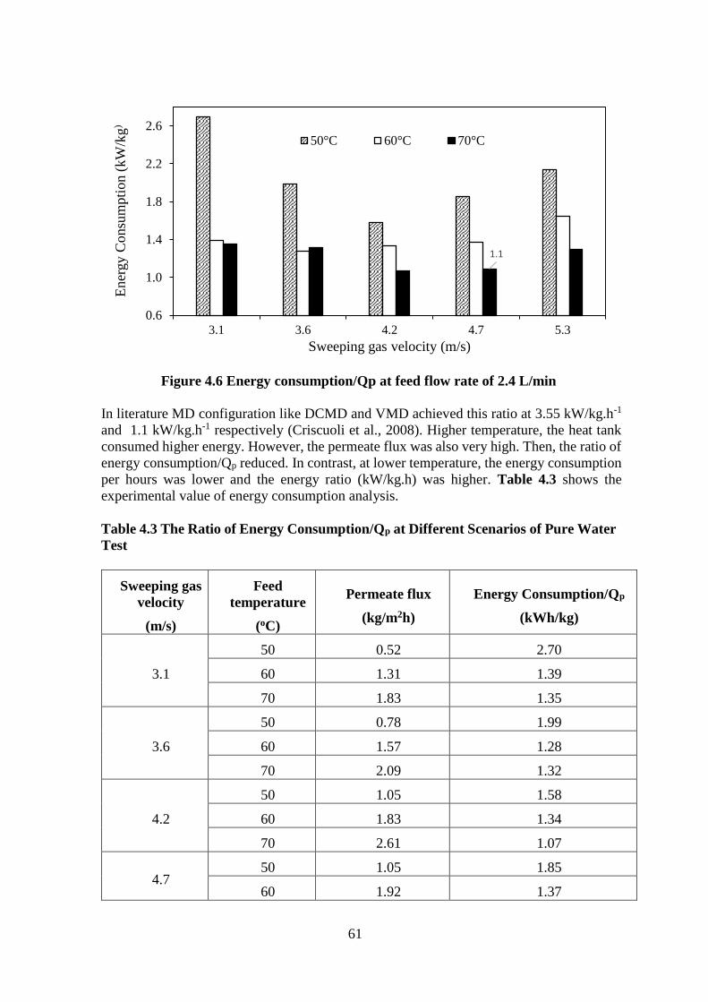
61
Figure 4.6 Energy consumption/Qp at feed flow rate of 2.4 L/min
In literature MD configuration like DCMD and VMD achieved this ratio at 3.55 kW/kg.h-1
and 1.1 kW/kg.h-1 respectively (Criscuoli et al., 2008). Higher temperature, the heat tank
consumed higher energy. However, the permeate flux was also very high. Then, the ratio of
energy consumption/Qp reduced. In contrast, at lower temperature, the energy consumption
per hours was lower and the energy ratio (kW/kg.h) was higher. Table 4.3 shows the
experimental value of energy consumption analysis.
Table 4.3 The Ratio of Energy Consumption/Qp at Different Scenarios of Pure Water
Test
Sweeping gas
velocity
(m/s)
Feed
temperature
(oC)
Permeate flux
(kg/m2h)
Energy Consumption/Qp
(kWh/kg)
3.1
50 0.52 2.70
60 1.31 1.39
70 1.83 1.35
3.6
50 0.78 1.99
60 1.57 1.28
70 2.09 1.32
4.2
50 1.05 1.58
60 1.83 1.34
70 2.61 1.07
4.7 50 1.05 1.85
60 1.92 1.37
1.1
0.6
1.0
1.4
1.8
2.2
2.6
3.1 3.6 4.2 4.7 5.3
Ener
gy C
onsu
mpti
on (
kW
/kg
)
Sweeping gas velocity (m/s)
50°C 60°C 70°C
62
70 3.14 1.09
5.3
50 1.05 2.14
60 1.57 1.64
70 2.7 1.30
Overall, the best condition in terms of balancing between energy consumption/Qp and
permeate flux were achieved at feed flow rate of 2.4 (L/min), feed temperature of 70oC, and
sweeping gas velocity of 4.7 m/s. At this condition, pure water flux achieved was 3.14
kg/m2.h, the ratio of energy consumption/Qp was 1.09 kW/kg. A comparison between pure
water flux obtained in this research and observed in literature is presented in Table 4.4.
4.3.1.4 Membrane coefficient and resistance
By using the result of pure water test, membrane coefficient (Bw) and membrane resistance
(Alkhudhiri et al., 2012) would be evaluated. Equation 2.1 shows the relationship between
permeate flux and membrane coefficient. Rw can be calculated by using Equation 4.1.
𝐑𝐰 =𝟏
𝐁𝐰 (4.1)
All operating temperatures used to calculate vapour pressure are temperature at membrane
surface (Tmf and Tmp) (Equation 4.3 and 4.4). This is due to the vaporization phenomena
taking place at the entrance of membrane pore. Thus, it is necessary to calculate Tmf and Tmp
to evaluate Bw more exactly. The procedure to calculate Tmf and Tmp is expressed as below
(Martı́nez-Dı́ez and Vázquez-González, 1999):
1) Calculate the value of Reynolds number (Re), Prandtl number (Pr) and Nusselt
number (Larpkiattaworn, 2013) at both feed side and permeate side. From those
values, heat transfer coefficient of boundary layer at feed surface (hf) and permeate
surface (hp) are evaluated.
2) Assume Tmf and Tmp then calculate the vapour heat transfer (hv) by Equation 4.2.
𝐡𝐯 =𝐉 × 𝛗
𝐓𝐦𝐟 − 𝐓𝐦𝐩
(4.2)
Where φ is the latent heat of water vapour evaporation (2270 kJ/kg).
3) Use the calculated hv to evaluate Tmf and Tmp by two Equations below:

63
Table 4.4 PWF Comparison with Other Studies on SGMD
Membrane type Gas velocity
(m/s)
Tf
(oC)
PWF
(kg/m2.h) Reference
Hollow fiber
(PTFE – 0.45µm)
3.1
50 0.52
This study
60 1.31
70 1.83
3.6
50 0.78
60 1.57
70 2.09
4.2
50 1.05
60 1.83
70 2.61
4.7
50 1.05
60 1.92
70 3.14
5.3
50 1.05
60 1.57
70 2.7
Hollow fiber (PTFE) 8.7 45 1.95 Lee and Hong,
2001
Flat sheet
(TF-200)
1.0 65 5.4
Khayet et al.,
2000
1.5 65 7.2
2 65 9.0
Flat sheet
(TF-450)
1.0 65 6.8
1.5 65 8.6
2 65 10.0
𝐓𝐦𝐟 = 𝐓𝐛𝐟 − (𝐓𝐛𝐟 − 𝐓𝐛𝐩) ×𝟏 𝐡𝐟⁄
𝟏 (𝐡𝐦 + 𝐡𝐯) + 𝟏 𝐡𝐟⁄ + 𝟏 𝐡𝐩⁄⁄ (4.3)
𝐓𝐦𝐩 = 𝐓𝐛𝐩 + (𝐓𝐛𝐟 − 𝐓𝐛𝐩) ×𝟏 𝐡𝐩⁄
𝟏 (𝐡𝐦 + 𝐡𝐯) + 𝟏 𝐡𝐟⁄ + 𝟏 𝐡𝐩⁄⁄ (4.4)
1) Repeat the procedure until the difference between the assumed calculated values
does not exceed 0.1%.

64
Tmf and Tmp are different from Tbf and Tbp due to the effect of flow condition and heat
transfer efficiency. This phenomena is named as temperature polarization. At Tbf = 69 and
Tbp =48 oC, Tmf and Tmp are 66.60 and 64.53oC respectively. The permeate temperate is
higher in the bulk than at the membrane surface is due to the fact heat transfer was occurring
from the feed side and also that air gains heat faster than liquids.
Table 4.5 Membrane Surface Temperature and Temperature Polarization Coefficient
Feed Permeate TPC
Tbf (oC) Tmf (oC) Tbp (oC) Tmp (oC)
69 66.6 48 64.5
0.1 59 57.2 43 55.6
49 47.7 38 46.6
*Remark: Tbf and Tbp are bulk feed and bulk permeate temperature.
Table 4.6 Experimental Membrane Distillation Coefficient and Membrane Resistance
Membrane Configuration Mass Transfer
Mechanism
Bw
(10-8 s/m)
Rw
(107 m/s)
Hollow fiber
PTFE
(0.45 µm)
SGMD
(This study) Knudsen and
Molecular
diffusion
combined
3.47 2.9
DCMD
(Yuthawong,
2014)
4.2 23.6
As presented in Table 4.6 membrane coefficient of hollow fiber PTFE (0.45µm) operating
with SGMD configuration was 3.47 x 10⁻⁸ s/m and was higher than while operating as
DCMD configuration. Yuthawong (2014) achieved Bw at 4.2 x 10⁻⁸ s/m. Implying that
hollow fiber PTFE MD had a higher permeability when operating with SGMD configuration
(lower membrane resistance).
4.3.2 Synthetic TEG
4.3.2.1 Batch experiments
Before investigating MD system with real TEG wastewater, it was important to test with
synthetic TEG wastewater. This experiment was aimed at investigating MD performance
with only TEG, without BTEX and any inorganic foulant. In synthetic wastewater test, the
effect of boundary layer resistance was also evaluated. Boundary layer was formed by the
appearance of TEG in feed solution. However, it theoretically creates less effect in SGMD
configuration (Khayet and Matsuura, 2011).
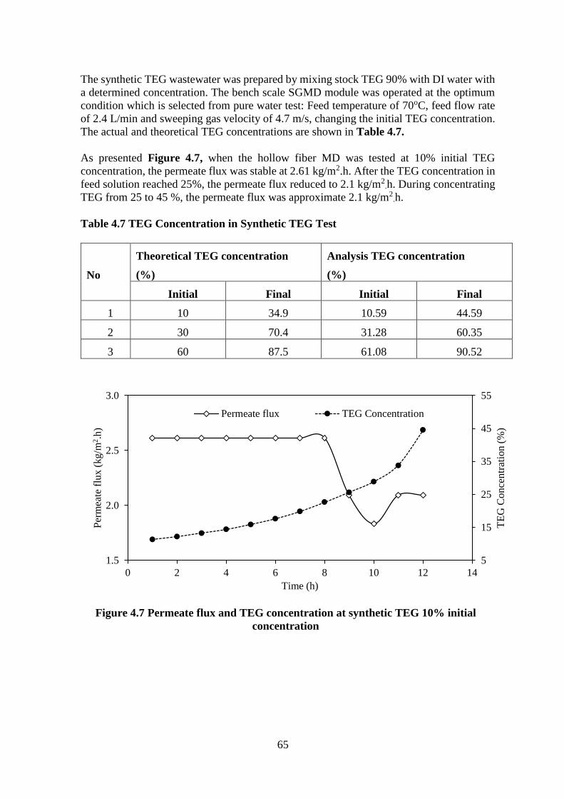
65
The synthetic TEG wastewater was prepared by mixing stock TEG 90% with DI water with
a determined concentration. The bench scale SGMD module was operated at the optimum
condition which is selected from pure water test: Feed temperature of 70oC, feed flow rate
of 2.4 L/min and sweeping gas velocity of 4.7 m/s, changing the initial TEG concentration.
The actual and theoretical TEG concentrations are shown in Table 4.7.
As presented Figure 4.7, when the hollow fiber MD was tested at 10% initial TEG
concentration, the permeate flux was stable at 2.61 kg/m2.h. After the TEG concentration in
feed solution reached 25%, the permeate flux reduced to 2.1 kg/m2.h. During concentrating
TEG from 25 to 45 %, the permeate flux was approximate 2.1 kg/m2.h.
Table 4.7 TEG Concentration in Synthetic TEG Test
No
Theoretical TEG concentration
(%)
Analysis TEG concentration
(%)
Initial Final Initial Final
1 10 34.9 10.59 44.59
2 30 70.4 31.28 60.35
3 60 87.5 61.08 90.52
Figure 4.7 Permeate flux and TEG concentration at synthetic TEG 10% initial
concentration
5
15
25
35
45
55
1.5
2.0
2.5
3.0
0 2 4 6 8 10 12 14
TE
G C
once
ntr
atio
n (
%)
Per
mea
te f
lux (
kg/m
2.h
)
Time (h)
Permeate flux TEG Concentration
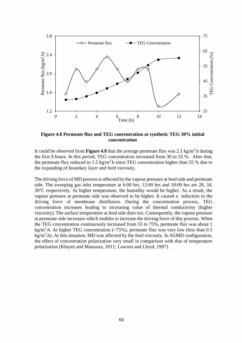
66
Figure 4.8 Permeate flux and TEG concentration at synthetic TEG 30% initial
concentration
It could be observed from Figure 4.8 that the average permeate flux was 2.1 kg/m2.h during
the first 9 hours. In this period, TEG concentration increased from 30 to 55 %. After that,
the permeate flux reduced to 1.5 kg/m2.h since TEG concentration higher than 55 % due to
the expanding of boundary layer and feed viscosity.
The driving force of MD process is affected by the vapour pressure at feed side and permeate
side. The sweeping gas inlet temperature at 6:00 hrs, 12:00 hrs and 18:00 hrs are 28, 34,
30oC respectively. At higher temperature, the humidity would be higher. As a result, the
vapour pressure at permeate side was observed to be higher. It caused a reduction in the
driving force of membrane distillation. During the concentration process, TEG
concentration increases leading to increasing value of thermal conductivity (higher
viscosity). The surface temperature at feed side does too. Consequently, the vapour pressure
at permeate side increases which enables to increase the driving force of this process. When
the TEG concentration continuously increased from 55 to 75%, permeate flux was about 1
kg/m2.h. At higher TEG concentration (>75%), permeate flux was very low (less than 0.5
kg/m2.h). At this situation, MD was affected by the feed viscosity. In SGMD configuration,
the effect of concentration polarization very small in comparison with that of temperature
polarization (Khayet and Matsuura, 2011; Lawson and Lloyd, 1997).
25
35
45
55
65
75
1.2
1.6
2.0
2.4
2.8
0 2 4 6 8 10 12 14
TE
G C
on
cen
trat
ion
(%
)
Per
mea
te f
lux
(kg/m
2.h
)
Time (h)
Permeate flux TEG Concentration

67
Figure 4.9 Permeate flux and TEG concentration at synthetic TEG 60% initial
concentration
4.3.2.2 Continuously-fed synthetic TEG experiment
Synthetic TEG (10%) was prepared by mixing stock TEG (90%) with DI water. It was used
to fill up the feed tank every 8 hours in this experiment. The TEG concentration reduced
dramatically at the moment of feeding by synthetic TEG 10%. However, its concentration
increased in whole process (from 10% to 53%) because of the continuous feeding progress.
All experimental results of this experiment is shown in Figure 4.10.
Figure 4.10 Experimental result of continuously-fed synthetic TEG investigation
55
65
75
85
95
0.0
0.4
0.8
1.2
1.6
0 5 10 15 20 25
TE
G C
on
cen
trat
ion
(%
)
Per
mea
te f
lux
(kg/m
2. h
)
Time (h)
Permeate flux TEG Concentration
5
15
25
35
45
55
1.5
2.0
2.5
3.0
0 10 20 30 40 50
TE
G c
on
cen
trat
ion(%
)
Per
mea
te f
lux (
kg/m
2.h
)
Time (h)
Permeate flux
TEG concentration
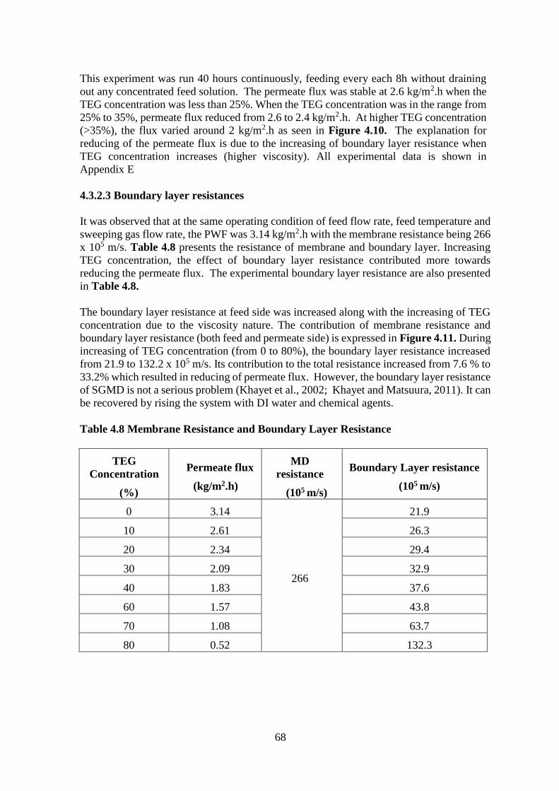
68
This experiment was run 40 hours continuously, feeding every each 8h without draining
out any concentrated feed solution. The permeate flux was stable at 2.6 kg/m2.h when the
TEG concentration was less than 25%. When the TEG concentration was in the range from
25% to 35%, permeate flux reduced from 2.6 to 2.4 kg/m2.h. At higher TEG concentration
(>35%), the flux varied around 2 kg/m2.h as seen in Figure 4.10. The explanation for
reducing of the permeate flux is due to the increasing of boundary layer resistance when
TEG concentration increases (higher viscosity). All experimental data is shown in
Appendix E
4.3.2.3 Boundary layer resistances
It was observed that at the same operating condition of feed flow rate, feed temperature and
sweeping gas flow rate, the PWF was 3.14 kg/m2.h with the membrane resistance being 266
x 105 m/s. Table 4.8 presents the resistance of membrane and boundary layer. Increasing
TEG concentration, the effect of boundary layer resistance contributed more towards
reducing the permeate flux. The experimental boundary layer resistance are also presented
in Table 4.8.
The boundary layer resistance at feed side was increased along with the increasing of TEG
concentration due to the viscosity nature. The contribution of membrane resistance and
boundary layer resistance (both feed and permeate side) is expressed in Figure 4.11. During
increasing of TEG concentration (from 0 to 80%), the boundary layer resistance increased
from 21.9 to 132.2 x 10⁵ m/s. Its contribution to the total resistance increased from 7.6 % to
33.2% which resulted in reducing of permeate flux. However, the boundary layer resistance
of SGMD is not a serious problem (Khayet et al., 2002; Khayet and Matsuura, 2011). It can
be recovered by rising the system with DI water and chemical agents.
Table 4.8 Membrane Resistance and Boundary Layer Resistance
TEG
Concentration
(%)
Permeate flux
(kg/m2.h)
MD
resistance
(105 m/s)
Boundary Layer resistance
(105 m/s)
0 3.14
266
21.9
10 2.61 26.3
20 2.34 29.4
30 2.09 32.9
40 1.83 37.6
60 1.57 43.8
70 1.08 63.7
80 0.52 132.3

69
Figure 4.11 Increasing of boundary layer resistance
The calculations of boundary layer resistance are expressed Appendix D
4.3.3 Bench scale with real TEG wastewater
Real wastewater was used to conduct the experiment on hollow fiber membrane after PWF
and synthetic TEG test. This experiment was aimed to evaluate the performance of SGMD
when operating with the real wastewater. Fouling analysis were conducted by checking the
PWF after cleaning the module with DI water and chemical agents. By operating the bench
scale hollow fiber module with real wastewater, it would be suitable to scale up the operating
condition for the pilot scale module, then designing of full scale plant. The operational
conditions of this experiment were feed flow rate of 2.4 L/min, feed temperature of 70oC
and sweeping gas velocity of 4.7 m/s.
4.3.3.1 Batch experiments
The real wastewater after treating by pre-treatment system was divided into 5 batches to
concentrate by SGMD system. The feed solution (real wastewater) was changed after each
batch without any system’s cleaning. By operating all experiments at the same condition
(sweeping gas flow rate of 0.255 L/min/fiber (4.7 m/s), feed temperature of 70oC and feed
flow rate of 2.4 L/min), the experimental results of Batch 1 and batch 5 are shown in Figure
4.12. After finishing 5 batches (total of 40 hours), fouling analysis was conducted to identify
different types of fouling.
50
60
70
80
90
100
0 10 20 30 40 60 70 80
Pro
po
rtio
n c
on
trib
uti
ng t
o r
esis
tan
ce
(%)
TEG concentration (%)
Membrane Resistance Boundary Layer Resistance
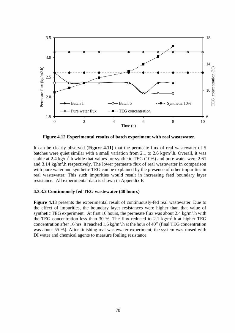
70
Figure 4.12 Experimental results of batch experiment with real wastewater.
It can be clearly observed (Figure 4.11) that the permeate flux of real wastewater of 5
batches were quiet similar with a small variation from 2.1 to 2.6 kg/m2.h. Overall, it was
stable at 2.4 kg/m2.h while that values for synthetic TEG (10%) and pure water were 2.61
and 3.14 kg/m2.h respectively. The lower permeate flux of real wastewater in comparison
with pure water and synthetic TEG can be explained by the presence of other impurities in
real wastewater. This such impurities would result in increasing feed boundary layer
resistance. All experimental data is shown in Appendix E
4.3.3.2 Continuously fed TEG wastewater (40 hours)
Figure 4.13 presents the experimental result of continuously-fed real wastewater. Due to
the effect of impurities, the boundary layer resistances were higher than that value of
synthetic TEG experiment. At first 16 hours, the permeate flux was about 2.4 kg/m2.h with
the TEG concentration less than 30 %. The flux reduced to 2.1 kg/m2.h at higher TEG
concentration after 16 hrs. It reached 1.6 kg/m2.h at the hour of 40th (final TEG concentration
was about 55 %). After finishing real wastewater experiment, the system was rinsed with
DI water and chemical agents to measure fouling resistance.
6
10
14
18
1.5
2.0
2.5
3.0
3.5
0 2 4 6 8 10
TE
G co
nce
ntr
atio
n (
%)
Per
mea
te f
lux
(k
g/m
2.h
)
Time (h)
Batch 1 Batch 5 Synthetic 10%
Pure water flux TEG concentration

71
Figure 4.13 Experimental result of continuously-fed real wastewater investigation
4.3.3.3 Continuously fed TEG wastewater (210 hours)
The real wastewater was continuously fill up to 10 L in the feed tank without draining any
concentrate. Figure 4.14 show the permeate flux of SGMD during 210 hours operating
continuously. This corresponds to 38 days of operation at 8 hours operation/day. It is clear
that the permeate flux was almost stable at 2.6 kg/m2.h within the first 60 hours. At the hour
in the range from 60 to 170, it reduced and stable at 2.3 kg/m2.h. After 170 hours of feeding
continuously, the permeate flux of membrane was stable at 1.5 kg/m2.h. Overall, the
permeate flux of SGMD after 210 hours operating continuously was reduced to 60% as
compared to the first hour. It proves that fouling phenomena is not a serious problem in MD
technology.
Figure 4.14 Permeate flux and TEG concentration during 210 hrs feeding
continuously
0
10
20
30
40
50
60
1.0
1.5
2.0
2.5
3.0
0 10 20 30 40 50
TE
G c
on
cen
trat
ion
(%)
Per
mea
te f
lux
(kg/m
2.h
)
Time (h)
Permeate flux TEG concentration
0
20
40
60
80
100
0.0
0.5
1.0
1.5
2.0
2.5
3.0
0 40 80 120 160 200 240
TE
G c
once
ntr
atio
n (
%)
Per
mea
te f
lux (
kg/m
2.h
)
Time (h)
Permeate flux
TEG Concentration
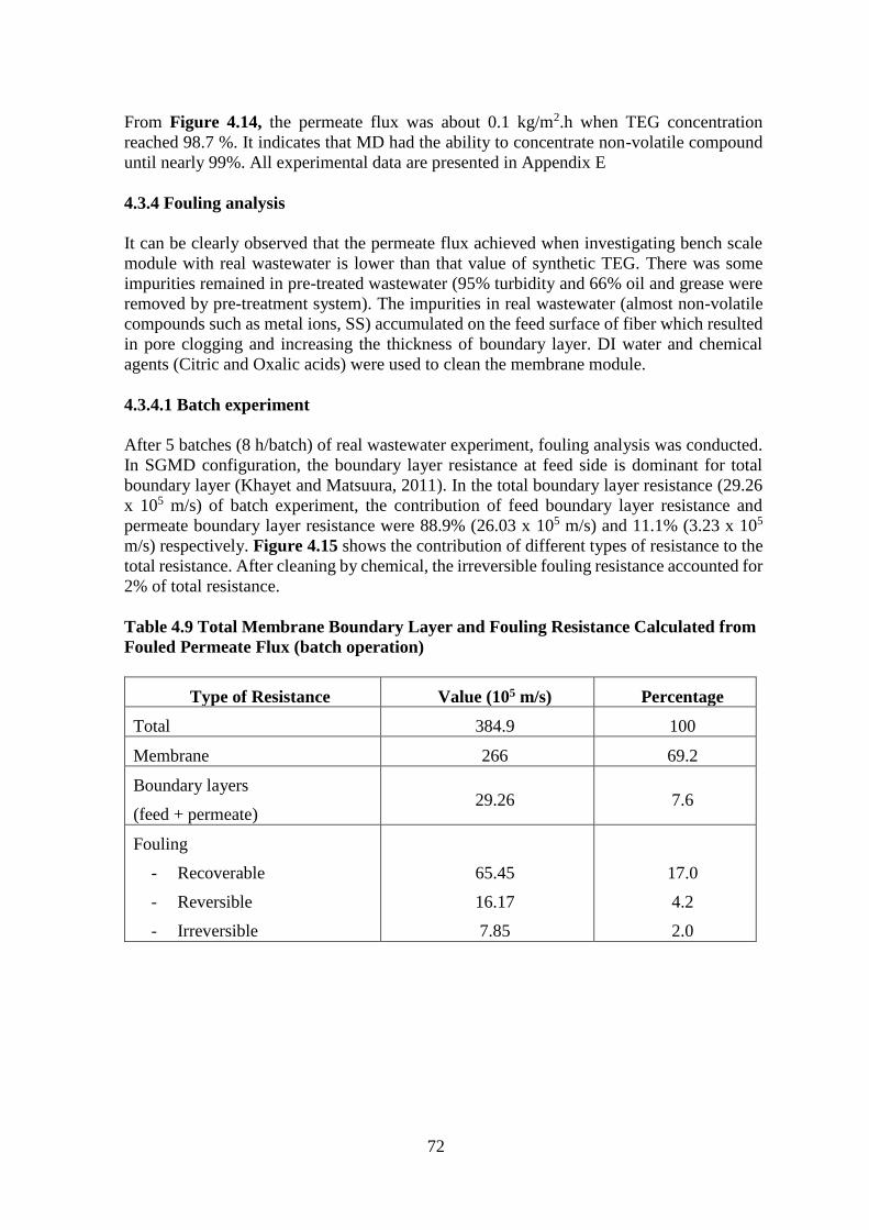
72
From Figure 4.14, the permeate flux was about 0.1 kg/m2.h when TEG concentration
reached 98.7 %. It indicates that MD had the ability to concentrate non-volatile compound
until nearly 99%. All experimental data are presented in Appendix E
4.3.4 Fouling analysis
It can be clearly observed that the permeate flux achieved when investigating bench scale
module with real wastewater is lower than that value of synthetic TEG. There was some
impurities remained in pre-treated wastewater (95% turbidity and 66% oil and grease were
removed by pre-treatment system). The impurities in real wastewater (almost non-volatile
compounds such as metal ions, SS) accumulated on the feed surface of fiber which resulted
in pore clogging and increasing the thickness of boundary layer. DI water and chemical
agents (Citric and Oxalic acids) were used to clean the membrane module.
4.3.4.1 Batch experiment
After 5 batches (8 h/batch) of real wastewater experiment, fouling analysis was conducted.
In SGMD configuration, the boundary layer resistance at feed side is dominant for total
boundary layer (Khayet and Matsuura, 2011). In the total boundary layer resistance (29.26
x 105 m/s) of batch experiment, the contribution of feed boundary layer resistance and
permeate boundary layer resistance were 88.9% (26.03 x 10⁵ m/s) and 11.1% (3.23 x 10⁵
m/s) respectively. Figure 4.15 shows the contribution of different types of resistance to the
total resistance. After cleaning by chemical, the irreversible fouling resistance accounted for
2% of total resistance.
Table 4.9 Total Membrane Boundary Layer and Fouling Resistance Calculated from
Fouled Permeate Flux (batch operation)
Type of Resistance Value (105 m/s) Percentage
Total 384.9 100
Membrane 266 69.2
Boundary layers
(feed + permeate) 29.26 7.6
Fouling
- Recoverable
- Reversible
- Irreversible
65.45
16.17
7.85
17.0
4.2
2.0

73
Figure 4.15 Classification of types of resistances in SGMD batch operation
4.3.4.2 Continuously-fed experiment
Similar to fouling analysis of batch experiment, the membrane module was also cleaned by
DI water and chemicals after operating 40 hrs continuously. In Figure 4.16, the contribution
of boundary layer resistance (30.9%) into the total resistance was higher than that value in
batch experiment (23.2%)
Table 4.10 Total Membrane Boundary Layer and Fouling Resistance Calculated from
Fouled Permeate Flux (continuously-fed operation)
Type of Resistance Value (105 m/s) Percentage
Total 432.8 100
Membrane 266 61.5
Boundary layers
(feed + permeate) 32.9 7.6
Fouling
- Recoverable
- Reversible
- Irreversible
109.7
16.17
7.85
25.3
3.7
1.8
Membrane
69.2 %
Boundary layer
7.6 %
Recoverable
17.0%
Reversible
4.2 %
Irreversible
2.0 %
Fouling
23.2 %
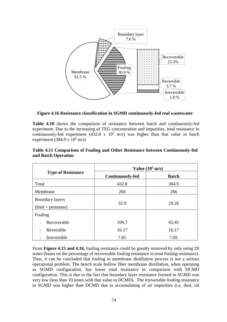
74
Figure 4.16 Resistance classification in SGMD continuously-fed real wastewater
Table 4.10 shows the comparison of resistance between batch and continuously-fed
experiment. Due to the increasing of TEG concentration and impurities, total resistance in
continuously-fed experiment (432.8 x 10⁵ m/s) was higher than that value in batch
experiment (384.9 x 10⁵ m/s)
Table 4.11 Comparison of Fouling and Other Resistance between Continuously-fed
and Batch Operation
Type of Resistance Value (105 m/s)
Continuously-fed Batch
Total 432.8 384.9
Membrane 266 266
Boundary layers
(feed + permeate) 32.9 29.26
Fouling
- Recoverable
- Reversible
- Irreversible
109.7
16.17
7.85
65.45
16.17
7.85
From Figure 4.15 and 4.16, fouling resistance could be greatly removed by only using DI
water (bases on the percentage of recoverable fouling resistance in total fouling resistance).
Thus, it can be concluded that fouling in membrane distillation process is not a serious
operational problem. The bench scale hollow fiber membrane distillation, when operating
as SGMD configuration, has lower total resistance in comparison with DCMD
configuration. This is due to the fact that boundary layer resistance formed in SGMD was
very low (less than 10 times with that value in DCMD). The irreversible fouling resistance
in SGMD was higher than DCMD due to accumulating of air impurities (i.e. dust, oil
Membrane
61.5 %
Boundary layer
7.6 %
Recoverable
25.3%
Reversible
3.7 %
Irreversible
1.8 %
Fouling
30.9 %

75
compound from compressor) at the permeate side of membrane. It could not be removed
during cleaning procedure. For DCMD, the permeate side could be rinsed with DI water.
Table 4.12 Comparison of Fouling and Other Resistance between SGMD and DCMD
Bench Scale Hollow Fiber Membrane Distillation (Continuously-fed)
Type of Resistance
Value (105 m/s)
SGMD
(This study)
DCMD
(Yuthawong, 2014)
Total 432.8 730
Membrane 266 236
Boundary layers
(feed + permeate) 32.9 418.4
Fouling
- Recoverable
- Reversible
- Irreversible
109.7
16.17
7.85
73
0
2.6
4.3.5 Evaluation of energy consumption of bench scale SGMD
To enhance the heat transfer efficiency, it was necessary to minimize the boundary layer
resistances (temperature polarization would be reduced consequently) (Criscuoli et al.,
2008). To maintain the driving force of SGMD process, the heat should be supplied into
feed solution and the sweeping gas should be pumped continuously into the hollow fiber.
These steps required energy consumption. In this study, the energy efficiency of operating
process was evaluated. This was the energy required to maintain the driving force in the
MD process after the system started.
There were 4 main components which consumed energy in bench scale SGMD system:
feed pump, heater, control box, and air compressor. The electricity consumptions of three
first components (feed pump, heater, control box) were measured by a power meter.
Meanwhile, the energy consumption of air compressor was calculated theoretically based
on amount of air delivered and the full load power of compressor. The calculations for
energy ratio are shown in Appendix F
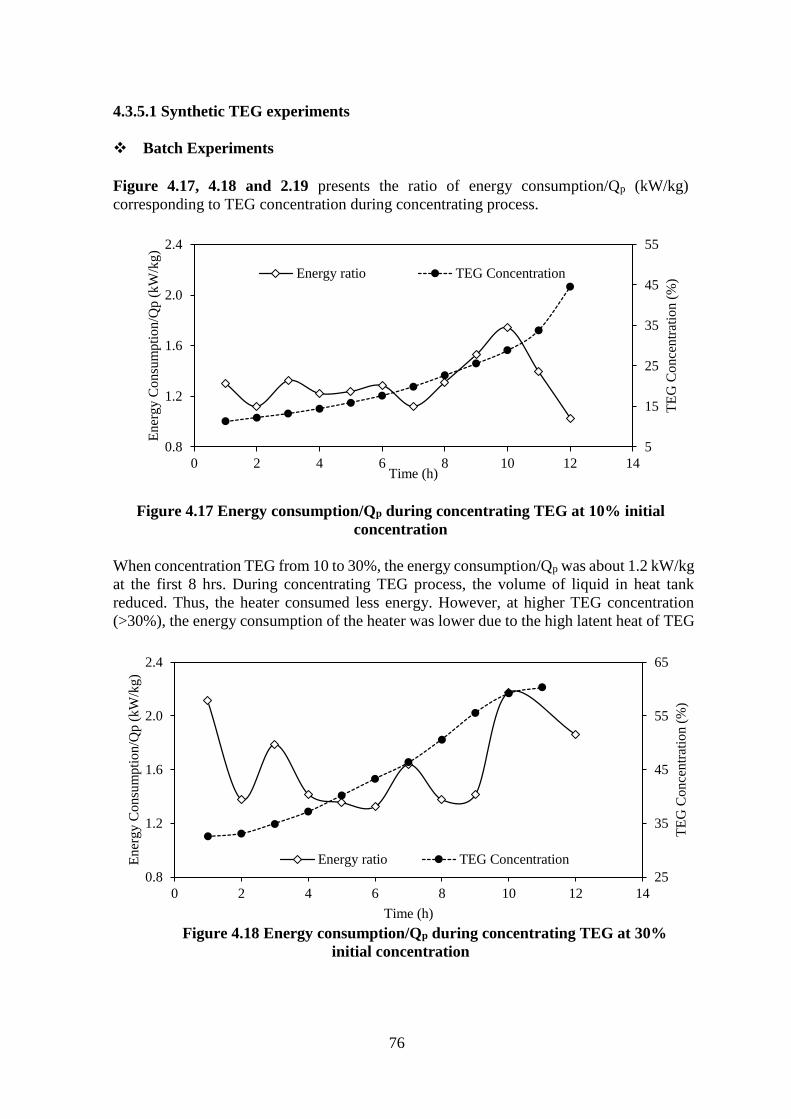
76
4.3.5.1 Synthetic TEG experiments
Batch Experiments
Figure 4.17, 4.18 and 2.19 presents the ratio of energy consumption/Qp (kW/kg)
corresponding to TEG concentration during concentrating process.
Figure 4.17 Energy consumption/Qp during concentrating TEG at 10% initial
concentration
When concentration TEG from 10 to 30%, the energy consumption/Qp was about 1.2 kW/kg
at the first 8 hrs. During concentrating TEG process, the volume of liquid in heat tank
reduced. Thus, the heater consumed less energy. However, at higher TEG concentration
(>30%), the energy consumption of the heater was lower due to the high latent heat of TEG
Figure 4.18 Energy consumption/Qp during concentrating TEG at 30%
initial concentration
5
15
25
35
45
55
0.8
1.2
1.6
2.0
2.4
0 2 4 6 8 10 12 14
TE
G C
on
cen
trat
ion
(%
)
En
erg
y C
on
sum
pti
on
/Qp
(k
W/k
g)
Time (h)
Energy ratio TEG Concentration
25
35
45
55
65
0.8
1.2
1.6
2.0
2.4
0 2 4 6 8 10 12 14
TE
G C
once
ntr
atio
n (
%)
Ener
gy C
onsu
mpti
on/Q
p (
kW
/kg)
Time (h)
Energy ratio TEG Concentration

77
Figure 4.19 Energy consumption/Qp During concentrating TEG at 60% initial
concentration
The permeate flux and energy consumption had small variation in every each hour. Thus,
the energy ratio was not stable but it showed a trend. At low TEG concentration, permeate
flux was very high. Thus, the ratio of energy consumption (kW/kgh-1) was very low.
Increasing TEG concentration, the flux reduced and pump consumed more power. Along
with operating timeline, the volume of feed aqueous solution in feed tank reduced which
leads to reducing power consumption of the heater. To be concluded, when TEG
concentration was in the range from 10 to 60%, the ratio of energy consumption/Qp was
approximately 1.46 kW/kgh-1. At the later period, the average value of energy ratio was
~3.39 kW/kgh-1.
Continuously-fed experiments
Figure 4.20 Energy consumption/Qp during concentrating TEG for 40 hours
50
60
70
80
90
100
2
3
4
5
0 5 10 15 20 25
TE
G C
once
ntr
atio
n (
%)
Ener
gy C
onsu
mpti
on/Q
p
(kW
/kg)
Time (h)
Energy ratio TEG Concentration
5
15
25
35
45
55
1.0
1.2
1.4
1.6
1.8
0 5 10 15 20 25 30 35 40
TE
G c
on
centr
atio
n(%
)
En
ergy C
on
sum
pti
on/Q
p(k
W/k
g)
Time (h)
Energy ratio TEG concentration

78
The energy consumption, the average ratio of energy consumption/ permeate flow when
concentrating TEG from 10 to 50 % was about 1.29 kWh/kg. It means that SGMD
configuration consumed less energy than DCMD (3.55 kWh/kg) and higher than VMD (1.1
kWh/kg) (Criscuoli et al., 2008).
4.3.5.2 Real wastewater experiment
Batch experiments
Figure 4.21 shows the comparison of energy consumption/ permeate flow between pure
water, synthetic TEG and real waste water. Due to the highest permeate flux in pure water
test (comparing with other feed solutions), the ratio of energy consumption/Qp of PWF
was lowest (1.09 kW/kg) while that value for real wastewater and synthetic TEG were
1.45 and 1.24 kW/kg respectively.
Figure 4.21 Energy consumption/Qp of batch experiment with real wastewater
The permeate flux at hour of 7th and 8th h in batch 5 reduced significantly. Thus, the energy
ratio of those hours increased very high.
Continuously-fed experiments
6
10
14
18
1.0
1.5
2.0
2.5
3.0
0 1 2 3 4 5 6 7 8T
EG
co
nce
ntr
atio
n (
%)
Ener
gy c
onsu
mpti
on/Q
p (
kW
/kg)
Time (h)
Batch 1 Batch 5
Synthetic 10% Pure water flux
TEG concentration
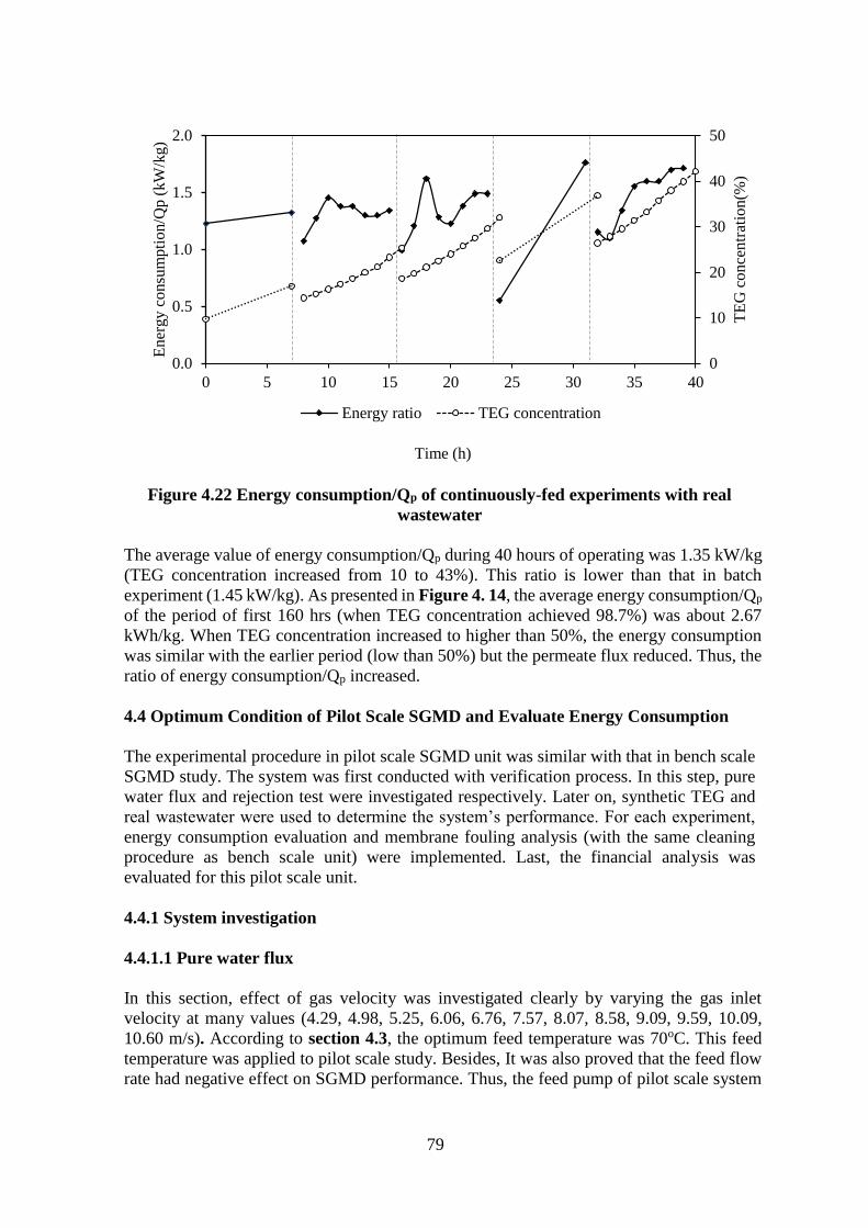
79
Figure 4.22 Energy consumption/Qp of continuously-fed experiments with real
wastewater
The average value of energy consumption/Qp during 40 hours of operating was 1.35 kW/kg
(TEG concentration increased from 10 to 43%). This ratio is lower than that in batch
experiment (1.45 kW/kg). As presented in Figure 4. 14, the average energy consumption/Qp
of the period of first 160 hrs (when TEG concentration achieved 98.7%) was about 2.67
kWh/kg. When TEG concentration increased to higher than 50%, the energy consumption
was similar with the earlier period (low than 50%) but the permeate flux reduced. Thus, the
ratio of energy consumption/Qp increased.
4.4 Optimum Condition of Pilot Scale SGMD and Evaluate Energy Consumption
The experimental procedure in pilot scale SGMD unit was similar with that in bench scale
SGMD study. The system was first conducted with verification process. In this step, pure
water flux and rejection test were investigated respectively. Later on, synthetic TEG and
real wastewater were used to determine the system’s performance. For each experiment,
energy consumption evaluation and membrane fouling analysis (with the same cleaning
procedure as bench scale unit) were implemented. Last, the financial analysis was
evaluated for this pilot scale unit.
4.4.1 System investigation
4.4.1.1 Pure water flux
In this section, effect of gas velocity was investigated clearly by varying the gas inlet
velocity at many values (4.29, 4.98, 5.25, 6.06, 6.76, 7.57, 8.07, 8.58, 9.09, 9.59, 10.09,
10.60 m/s). According to section 4.3, the optimum feed temperature was 70oC. This feed
temperature was applied to pilot scale study. Besides, It was also proved that the feed flow
rate had negative effect on SGMD performance. Thus, the feed pump of pilot scale system
0
10
20
30
40
50
0.0
0.5
1.0
1.5
2.0
0 5 10 15 20 25 30 35 40
TE
G c
on
cen
trat
ion
(%)
En
ergy c
on
sum
pti
on
/Qp
(kW
/kg)
Time (h)
Energy ratio TEG concentration

80
was operated at normal capacity (60L/min). Table 4.13 shows the experimental results of
pure water flux (PWF) investigation on pilot scale module.
The highest permeate flux that could be achieved in pilot scale was 1.99 kg/m2.h at the gas
velocity inside each fiber of 10.09 m/s (gas inlet flow rate of 0.57 L/min.fiber). For the
bench scale module, that value was 3.14 kg/m2.h at the gas velocity inside each fiber of 4.7
m/s (gas inlet flow rate of 0.255 L/min.fiber). It could be concluded that the fiber’s length
had a significant effect on SGMD process. The temperature profile of sweeping gas relied
along the length. The relationship between PWF and the ratio of energy consumption/Qp is
simulated in Figure 4.23. At higher gas velocity, the fiber has a greater opportunity of be
wetted. The hydrostatic pressure which was created by high sweeping gas velocity could
suck the feed liquid througout the membrane pores. The local permeate flux 𝐽𝑖(𝑥) along the
module length (L) can be calculated by using Equation 4.5 (Khayet and Matsuura, 2011).
𝐽𝑖 =1
𝐿∫ 𝐽𝑖(𝑥). 𝑑𝑥
𝐿
𝑜 (4.5)
The temperature varied along the length of fiber. The local temperature depends strongly on
the gas inlet flow rate. Thus, it is necessary to determine the profile of temperature and
vapour pressure along the membrane module length. Then, the local driving force would be
evaluated. The optimum condition was decided at the gas velocity of 8.07 m/s (gas inlet
flow rate of 0.44 L/min.fiber), feed inlet temperature of 70oC. Feed flow rate and sweeping
gas temperature have less effect. The flux achieved at this conditions was 1.94 kg/m2.h. At
this operating condition, the pressure at both feed side and permeate side was kept constant
at 0.4 bar. All experiment data is provided in Appendix E
Figure 4.23 Pure water flux at different sweeping gas inlet flow rate of pilot scale
study
0.3
0.4
0.5
0.6
0.7
0.8
0.5
1.0
1.5
2.0
2.5
4.0 5.0 6.0 7.0 8.0 9.0 10.0 11.0
En
ergy c
onsu
mpti
on (
kW
/kg)
Per
mea
te f
lux (
kg/m
2.h
)
Gas inlet flow rate per fiber (L/min)
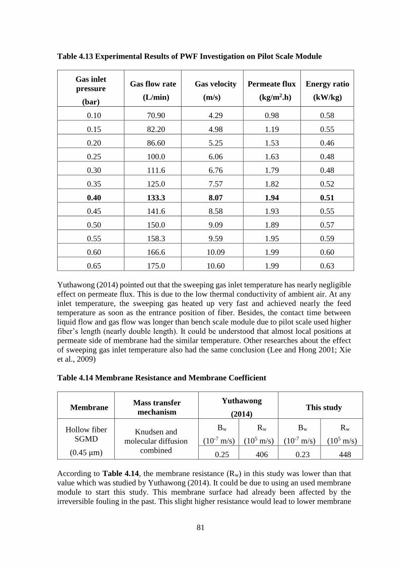
81
Table 4.13 Experimental Results of PWF Investigation on Pilot Scale Module
Gas inlet
pressure
(bar)
Gas flow rate
(L/min)
Gas velocity
(m/s)
Permeate flux
(kg/m2.h)
Energy ratio
(kW/kg)
0.10 70.90 4.29 0.98 0.58
0.15 82.20 4.98 1.19 0.55
0.20 86.60 5.25 1.53 0.46
0.25 100.0 6.06 1.63 0.48
0.30 111.6 6.76 1.79 0.48
0.35 125.0 7.57 1.82 0.52
0.40 133.3 8.07 1.94 0.51
0.45 141.6 8.58 1.93 0.55
0.50 150.0 9.09 1.89 0.57
0.55 158.3 9.59 1.95 0.59
0.60 166.6 10.09 1.99 0.60
0.65 175.0 10.60 1.99 0.63
Yuthawong (2014) pointed out that the sweeping gas inlet temperature has nearly negligible
effect on permeate flux. This is due to the low thermal conductivity of ambient air. At any
inlet temperature, the sweeping gas heated up very fast and achieved nearly the feed
temperature as soon as the entrance position of fiber. Besides, the contact time between
liquid flow and gas flow was longer than bench scale module due to pilot scale used higher
fiber’s length (nearly double length). It could be understood that almost local positions at
permeate side of membrane had the similar temperature. Other researches about the effect
of sweeping gas inlet temperature also had the same conclusion (Lee and Hong 2001; Xie
et al., 2009)
Table 4.14 Membrane Resistance and Membrane Coefficient
Membrane Mass transfer
mechanism
Yuthawong
(2014)
This study
Hollow fiber
SGMD
(0.45 µm)
Knudsen and
molecular diffusion
combined
Bw
(10-7 m/s)
Rw
(105 m/s)
Bw
(10-7 m/s)
Rw
(105 m/s)
0.25 406 0.23 448
According to Table 4.14, the membrane resistance (Rw) in this study was lower than that
value which was studied by Yuthawong (2014). It could be due to using an used membrane
module to start this study. This membrane surface had already been affected by the
irreversible fouling in the past. This slight higher resistance would lead to lower membrane
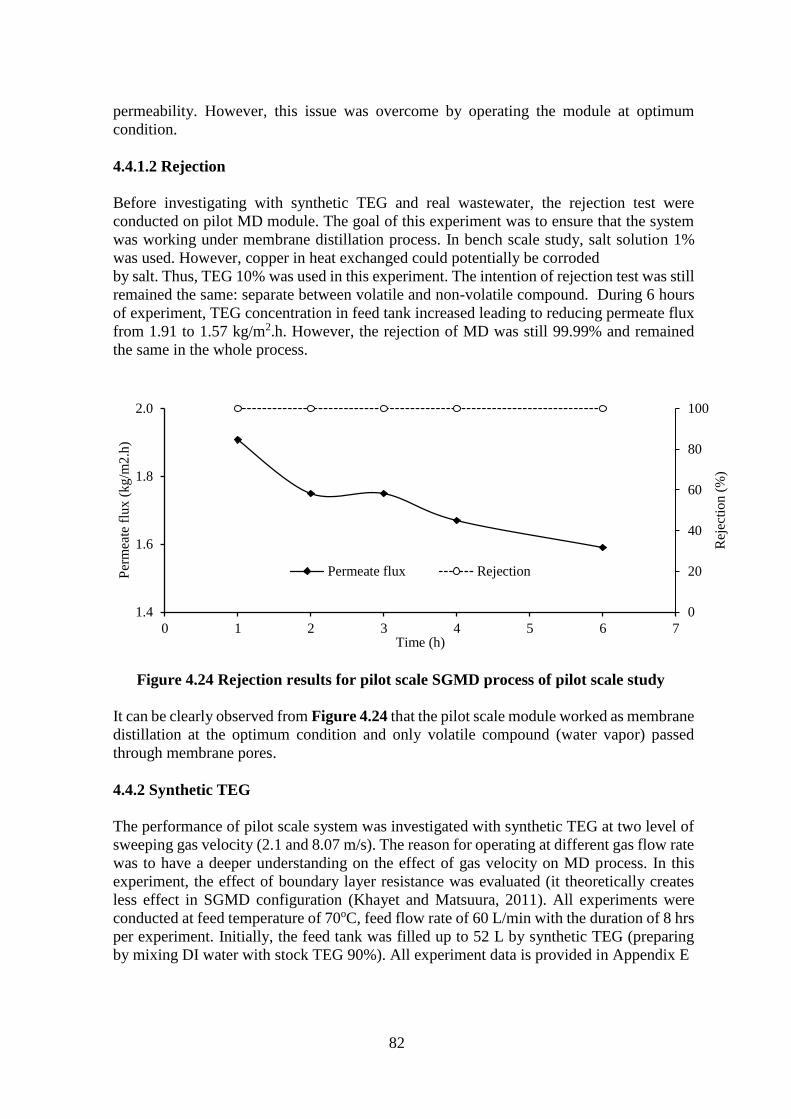
82
permeability. However, this issue was overcome by operating the module at optimum
condition.
4.4.1.2 Rejection
Before investigating with synthetic TEG and real wastewater, the rejection test were
conducted on pilot MD module. The goal of this experiment was to ensure that the system
was working under membrane distillation process. In bench scale study, salt solution 1%
was used. However, copper in heat exchanged could potentially be corroded
by salt. Thus, TEG 10% was used in this experiment. The intention of rejection test was still
remained the same: separate between volatile and non-volatile compound. During 6 hours
of experiment, TEG concentration in feed tank increased leading to reducing permeate flux
from 1.91 to 1.57 kg/m2.h. However, the rejection of MD was still 99.99% and remained
the same in the whole process.
Figure 4.24 Rejection results for pilot scale SGMD process of pilot scale study
It can be clearly observed from Figure 4.24 that the pilot scale module worked as membrane
distillation at the optimum condition and only volatile compound (water vapor) passed
through membrane pores.
4.4.2 Synthetic TEG
The performance of pilot scale system was investigated with synthetic TEG at two level of
sweeping gas velocity (2.1 and 8.07 m/s). The reason for operating at different gas flow rate
was to have a deeper understanding on the effect of gas velocity on MD process. In this
experiment, the effect of boundary layer resistance was evaluated (it theoretically creates
less effect in SGMD configuration (Khayet and Matsuura, 2011). All experiments were
conducted at feed temperature of 70oC, feed flow rate of 60 L/min with the duration of 8 hrs
per experiment. Initially, the feed tank was filled up to 52 L by synthetic TEG (preparing
by mixing DI water with stock TEG 90%). All experiment data is provided in Appendix E
0
20
40
60
80
100
1.4
1.6
1.8
2.0
0 1 2 3 4 5 6 7
Rej
ecti
on (
%)
Per
mea
te f
lux
(kg
/m2.h
)
Time (h)
Permeate flux Rejection
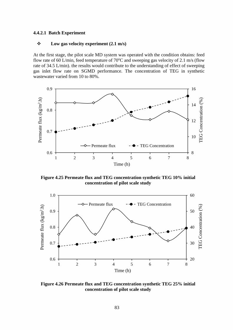
83
4.4.2.1 Batch Experiment
Low gas velocity experiment (2.1 m/s)
At the first stage, the pilot scale MD system was operated with the condition obtains: feed
flow rate of 60 L/min, feed temperature of 70oC and sweeping gas velocity of 2.1 m/s (flow
rate of 34.5 L/min). the results would contribute to the understanding of effect of sweeping
gas inlet flow rate on SGMD performance. The concentration of TEG in synthetic
wastewater varied from 10 to 80%.
Figure 4.25 Permeate flux and TEG concentration synthetic TEG 10% initial
concentration of pilot scale study
Figure 4.26 Permeate flux and TEG concentration synthetic TEG 25% initial
concentration of pilot scale study
8
10
12
14
16
0.6
0.7
0.8
0.9
1 2 3 4 5 6 7 8
TE
G C
on
centr
atio
n (
%)
Per
mea
te f
lux
(kg/m
2.h
)
Time (h)
Permeate flux TEG Concentration
20
30
40
50
60
0.6
0.7
0.8
0.9
1.0
1 2 3 4 5 6 7 8
TE
G C
once
ntr
atio
n (
%)
Per
mea
te f
lux
(kg/m
2.h
)
Time (h)
Permeate flux TEG Concentration
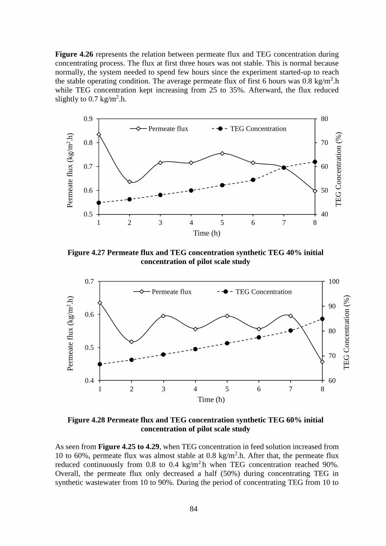
84
Figure 4.26 represents the relation between permeate flux and TEG concentration during
concentrating process. The flux at first three hours was not stable. This is normal because
normally, the system needed to spend few hours since the experiment started-up to reach
the stable operating condition. The average permeate flux of first 6 hours was 0.8 kg/m2.h
while TEG concentration kept increasing from 25 to 35%. Afterward, the flux reduced
slightly to 0.7 kg/m2.h.
Figure 4.27 Permeate flux and TEG concentration synthetic TEG 40% initial
concentration of pilot scale study
Figure 4.28 Permeate flux and TEG concentration synthetic TEG 60% initial
concentration of pilot scale study
As seen from Figure 4.25 to 4.29, when TEG concentration in feed solution increased from
10 to 60%, permeate flux was almost stable at 0.8 kg/m2.h. After that, the permeate flux
reduced continuously from 0.8 to 0.4 kg/m2.h when TEG concentration reached 90%.
Overall, the permeate flux only decreased a half (50%) during concentrating TEG in
synthetic wastewater from 10 to 90%. During the period of concentrating TEG from 10 to
40
50
60
70
80
0.5
0.6
0.7
0.8
0.9
1 2 3 4 5 6 7 8
TE
G C
once
ntr
atio
n (
%)
Per
mea
te f
lux
(kg/m
2.h
)
Time (h)
Permeate flux TEG Concentration
60
70
80
90
100
0.4
0.5
0.6
0.7
1 2 3 4 5 6 7 8
TE
G C
once
ntr
atio
n (
%)
Per
mea
te f
lux
(kg/m
2.h
)
Time (h)
Permeate flux TEG Concentration

85
80% (about 50 first hours), the ratio of energy consumption/Qp was about 0.6 kW/kg. At
higher TEG concentration, it rapidly increased (7 kW/kg at TEG concentration of 99%).
Figure 4.29 Permeate flux and TEG concentration synthetic TEG 80% initial
concentration of pilot scale study
Optimum gas velocity experiment (8.07 m/s)
In this scenario, the pilot scale MD system was investigated with the optimum gas velocity
(8.07 m/s). This condition was selected from the pure water test (balancing between
permeate flux and energy consumption). Synthetic TEG was used as feed solution at
different initial concentration (by mixing stock TEG 90% with DI water). Due to effect of
fiber’s length, the results from this experiment showed the limitation of pilot scale hollow
fiber module in comparison with bench scale experiments. Figure 4.30 presents the
experimental results of first synthetic TEG experiment at 10% initial concentration.
Figure 4.30 Permeate flux and TEG concentration synthetic TEG 10% initial
concentration of pilot scale study
75
80
85
90
95
100
0.0
0.2
0.4
0.6
0.8
1 3 5 7 9 11 13
TE
G C
once
ntr
atio
n (
%)
Per
mea
te f
lux
(kg/m
2.h
)
Time (h)
Permeate flux TEG Concentration
y = -0.0227x + 1.8363
R² = 0.4442
y = 1.4933x + 8.4478
R² = 0.96379
12
15
18
21
24
1.0
1.2
1.4
1.6
1.8
2.0
1 2 3 4 5 6 7 8
TE
G c
on
cen
trat
ion (
%)
Per
mea
te f
lux
(kg/m
2.h
)
Time (h)
Permeate flux TEG concentration

86
At the first hours of operating (initial TEG concentration of 10%), the permeate flux
achieved was 1.9 kg/m2.h. However, the permeate flux reduced in the following hours due
to the effect of concentration polarization. It decreased from 1.91 to 1.7 kg/m2.h, after 8 hrs
operating continuously. At the 8th hours, TEG concentration reached 21%. Implying 50%
of the volume was removed.
Figure 4.31 Permeate flux and TEG concentration synthetic TEG 20% initial
concentration of pilot scale study
At the second batch, TEG concentration at the initial hour was similar with the final
concentration Figure 4.31 (about 20%). However, the effect of concentration polarization
was very less at first hour. Thus, the flux still reached 1.8 kg/m2.h. At the 8th hours, TEG
concentration reached 41 % with the flux of 1.51 kg/m2.h. Once the concentration increased,
the effect of concentration polarization became more evident. The latent heat of TEG
compound is higher than that of water. Thus, the surface temperature at the feed side
increased. Besides, thermal conductivity also increased along with increasing TEG
concentration (effect of viscosity).
y = -0.03x + 1.7824
R² = 0.5968y = 2.7106x + 17.356
R² = 0.971315
20
25
30
35
40
45
1.0
1.2
1.4
1.6
1.8
2.0
1 2 3 4 5 6 7 8
TE
G c
on
cen
trat
ion
(%
)
Per
mea
te f
lux (
kg/m
2.h
)
Time (h)
Permeate flux TEG Concentration

87
Figure 4.32 Permeate flux and TEG concentration synthetic TEG 30% initial
concentration of pilot scale study
Figure 4.33 Permeate flux and TEG concentration synthetic TEG 40% initial
concentration of pilot scale study
When TEG concentration increased from 30 to 70%, permeate flux reduced slightly from
1.6 to 1.2 kg/m2.h. as seen in Figure 4.32. But while increasing the initial TEG concentration
to 40% and 60%, the flux was strongly affected by TEG concentration due to its viscosity
nature as presented in Figure 4.33. After the 6th hour the flux decline could be observed.
y = -0.0327x + 1.7121
R² = 0.729y = 3.6805x + 26.666
R² = 0.977425
35
45
55
65
1.0
1.2
1.4
1.6
1.8
2.0
1 2 3 4 5 6 7 8
TE
G c
on
cen
trat
ion
(%
)
Per
mea
te f
lux
(kg/m
2.h
)
Time (h)
Permeate flux TEG Concentration
y = -0.0381x + 1.59
R² = 0.9083
y = 4.0748x + 36.899
R² = 0.985335
45
55
65
75
1.0
1.2
1.4
1.6
1.8
1 2 3 4 5 6 7 8
TE
G c
once
ntr
atio
n (
%)
Per
mea
te f
lux
(kg/m
2.h
)
Time (h)
Permeate flux TEG Concentration
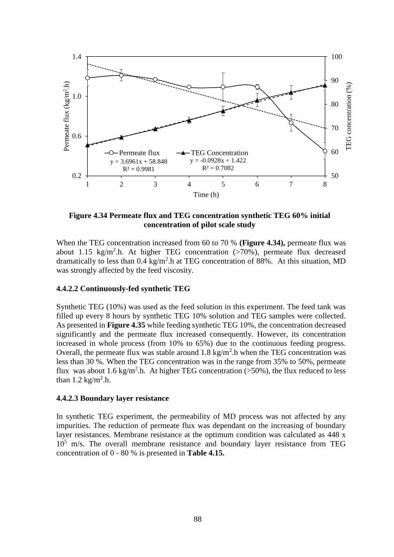
88
Figure 4.34 Permeate flux and TEG concentration synthetic TEG 60% initial
concentration of pilot scale study
When the TEG concentration increased from 60 to 70 % (Figure 4.34), permeate flux was
about 1.15 kg/m2.h. At higher TEG concentration (>70%), permeate flux decreased
dramatically to less than 0.4 kg/m2.h at TEG concentration of 88%. At this situation, MD
was strongly affected by the feed viscosity.
4.4.2.2 Continuously-fed synthetic TEG
Synthetic TEG (10%) was used as the feed solution in this experiment. The feed tank was
filled up every 8 hours by synthetic TEG 10% solution and TEG samples were collected.
As presented in Figure 4.35 while feeding synthetic TEG 10%, the concentration decreased
significantly and the permeate flux increased consequently. However, its concentration
increased in whole process (from 10% to 65%) due to the continuous feeding progress.
Overall, the permeate flux was stable around 1.8 kg/m2.h when the TEG concentration was
less than 30 %. When the TEG concentration was in the range from 35% to 50%, permeate
flux was about 1.6 kg/m2.h. At higher TEG concentration (>50%), the flux reduced to less
than 1.2 kg/m2.h.
4.4.2.3 Boundary layer resistance
In synthetic TEG experiment, the permeability of MD process was not affected by any
impurities. The reduction of permeate flux was dependant on the increasing of boundary
layer resistances. Membrane resistance at the optimum condition was calculated as 448 x
105 m/s. The overall membrane resistance and boundary layer resistance from TEG
concentration of 0 - 80 % is presented in Table 4.15.
y = -0.0928x + 1.422
R² = 0.7082y = 3.6961x + 58.848
R² = 0.998150
60
70
80
90
100
0.2
0.6
1.0
1.4
1 2 3 4 5 6 7 8
TE
G c
on
cen
trat
ion
(%
)
Per
mea
te f
lux
(kg/m
2.h
)
Time (h)
Permeate flux TEG Concentration
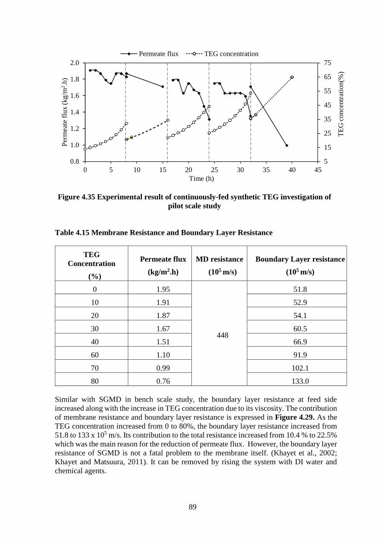
89
Figure 4.35 Experimental result of continuously-fed synthetic TEG investigation of
pilot scale study
Table 4.15 Membrane Resistance and Boundary Layer Resistance
TEG
Concentration
(%)
Permeate flux
(kg/m2.h)
MD resistance
(105 m/s)
Boundary Layer resistance
(105 m/s)
0 1.95
448
51.8
10 1.91 52.9
20 1.87 54.1
30 1.67 60.5
40 1.51 66.9
60 1.10 91.9
70 0.99 102.1
80 0.76 133.0
Similar with SGMD in bench scale study, the boundary layer resistance at feed side
increased along with the increase in TEG concentration due to its viscosity. The contribution
of membrane resistance and boundary layer resistance is expressed in Figure 4.29. As the
TEG concentration increased from 0 to 80%, the boundary layer resistance increased from
51.8 to 133 x 105 m/s. Its contribution to the total resistance increased from 10.4 % to 22.5%
which was the main reason for the reduction of permeate flux. However, the boundary layer
resistance of SGMD is not a fatal problem to the membrane itself. (Khayet et al., 2002;
Khayet and Matsuura, 2011). It can be removed by rising the system with DI water and
chemical agents.
5
15
25
35
45
55
65
75
0.8
1.0
1.2
1.4
1.6
1.8
2.0
0 5 10 15 20 25 30 35 40 45
TE
G c
on
cen
trat
ion
(%)
Per
mea
te f
lux
(kg/m
2.h
)
Time (h)
Permeate flux TEG concentration
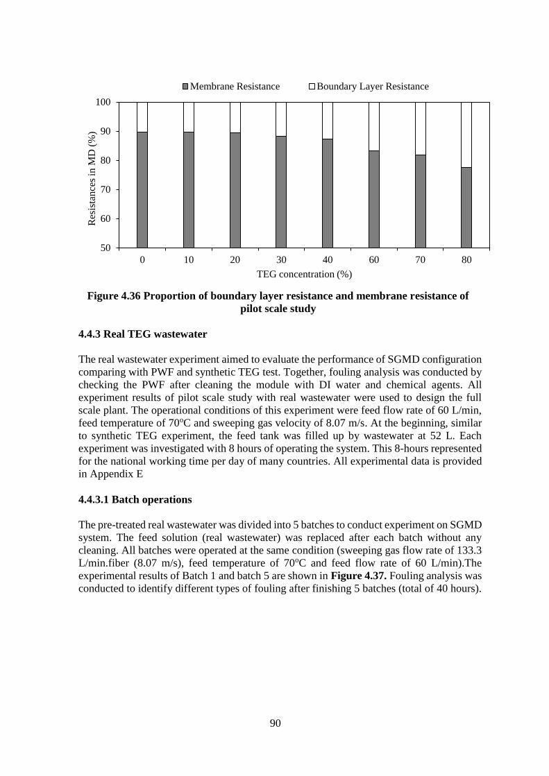
90
Figure 4.36 Proportion of boundary layer resistance and membrane resistance of
pilot scale study
4.4.3 Real TEG wastewater
The real wastewater experiment aimed to evaluate the performance of SGMD configuration
comparing with PWF and synthetic TEG test. Together, fouling analysis was conducted by
checking the PWF after cleaning the module with DI water and chemical agents. All
experiment results of pilot scale study with real wastewater were used to design the full
scale plant. The operational conditions of this experiment were feed flow rate of 60 L/min,
feed temperature of 70oC and sweeping gas velocity of 8.07 m/s. At the beginning, similar
to synthetic TEG experiment, the feed tank was filled up by wastewater at 52 L. Each
experiment was investigated with 8 hours of operating the system. This 8-hours represented
for the national working time per day of many countries. All experimental data is provided
in Appendix E
4.4.3.1 Batch operations
The pre-treated real wastewater was divided into 5 batches to conduct experiment on SGMD
system. The feed solution (real wastewater) was replaced after each batch without any
cleaning. All batches were operated at the same condition (sweeping gas flow rate of 133.3
L/min.fiber (8.07 m/s), feed temperature of 70oC and feed flow rate of 60 L/min).The
experimental results of Batch 1 and batch 5 are shown in Figure 4.37. Fouling analysis was
conducted to identify different types of fouling after finishing 5 batches (total of 40 hours).
50
60
70
80
90
100
0 10 20 30 40 60 70 80
Res
ista
nce
s in
MD
(%
)
TEG concentration (%)
Membrane Resistance Boundary Layer Resistance
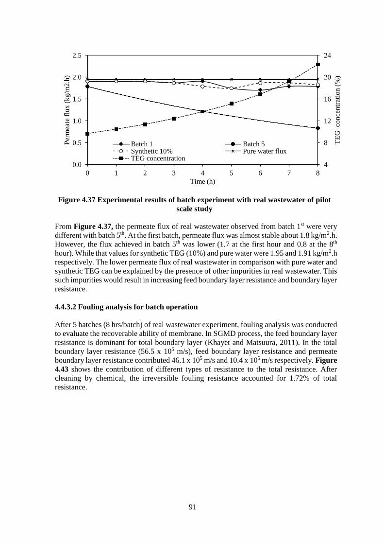
91
Figure 4.37 Experimental results of batch experiment with real wastewater of pilot
scale study
From Figure 4.37, the permeate flux of real wastewater observed from batch 1st were very
different with batch 5th. At the first batch, permeate flux was almost stable about 1.8 kg/m2.h.
However, the flux achieved in batch 5th was lower (1.7 at the first hour and 0.8 at the 8th
hour). While that values for synthetic TEG (10%) and pure water were 1.95 and 1.91 kg/m2.h
respectively. The lower permeate flux of real wastewater in comparison with pure water and
synthetic TEG can be explained by the presence of other impurities in real wastewater. This
such impurities would result in increasing feed boundary layer resistance and boundary layer
resistance.
4.4.3.2 Fouling analysis for batch operation
After 5 batches (8 hrs/batch) of real wastewater experiment, fouling analysis was conducted
to evaluate the recoverable ability of membrane. In SGMD process, the feed boundary layer
resistance is dominant for total boundary layer (Khayet and Matsuura, 2011). In the total
boundary layer resistance (56.5 x 10⁵ m/s), feed boundary layer resistance and permeate
boundary layer resistance contributed 46.1 x 10⁵ m/s and 10.4 x 10⁵ m/s respectively. Figure
4.43 shows the contribution of different types of resistance to the total resistance. After
cleaning by chemical, the irreversible fouling resistance accounted for 1.72% of total
resistance.
4
8
12
16
20
24
0.0
0.5
1.0
1.5
2.0
2.5
0 1 2 3 4 5 6 7 8
TE
G co
nce
ntr
atio
n (
%)
Per
mea
te f
lux
(kg/m
2.h
)
Time (h)
Batch 1 Batch 5Synthetic 10% Pure water fluxTEG concentration
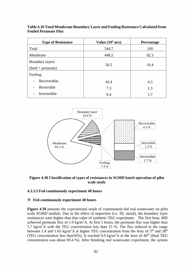
92
Table 4.16 Total Membrane Boundary Layer and Fouling Resistance Calculated from
Fouled Permeate Flux
Type of Resistance Value (105 m/s) Percentage
Total 544.7 100
Membrane 448.2 82.3
Boundary layers
(feed + permeate) 56.5 10.4
Fouling
- Recoverable
- Reversible
- Irreversible
43.4
7.3
9.4
4.3
1.3
1.7
Figure 4.38 Classification of types of resistances in SGMD batch operation of pilot
scale study
4.3.3.3 Fed-continuously experiment 40 hours
Fed-continuously experiment 40 hours
Figure 4.39 presents the experimental result of continuously-fed real wastewater on pilot
scale SGMD module. Due to the effect of impurities (i.e. SS, metal), the boundary layer
resistances were higher than that value of synthetic TEG experiment. The first hour, MD
achieved permeate flux of 1.9 kg/m2.h. At first 5 hours, the permeate flux was higher than
1.7 kg/m2.h with the TEG concentration less than 15 %. The flux reduced to the range
between 1.4 and 1.65 kg/m2.h at higher TEG concentration from the hour of 5th and 28th
(TEG concentration less than50%). It reached 0.9 kg/m2.h at the hour of 40th (final TEG
concentration was about 69.4 %). After finishing real wastewater experiment, the system
Membrane
82.3 %
Boundary layer
10.4 %
Recoverable
4.3 %
Reversible
1.3 %
Irreversible
1.7 %Fouling
7.4 %
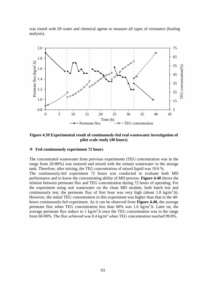
93
was rinsed with DI water and chemical agents to measure all types of resistance (fouling
analysis).
Figure 4.39 Experimental result of continuously-fed real wastewater investigation of
pilot scale study (40 hours)
Fed-continuously experiment 72 hours
The concentrated wastewater from previous experiments (TEG concentration was in the
range from 20-80%) was restored and mixed with the remain wastewater in the storage
tank. Therefore, after mixing, the TEG concentration of mixed liquid was 19.6 %.
The continuously-fed experiment 72 hours was conducted to evaluate both MD
performance and to know the concentrating ability of MD process. Figure 4.40 shows the
relation between permeate flux and TEG concentration during 72 hours of operating. For
the experiment using real wastewater on the clean MD module, both batch test and
continuously test, the permeate flux of first hour was very high (about 1.8 kg/m2.h).
However, the initial TEG concentration in this experiment was higher than that in the 40-
hours continuously-fed experiment. As it can be observed from Figure 4.40, the average
permeate flux when TEG concentration less than 60% was 1.6 kg/m2.h. Later on, the
average permeate flux reduce to 1 kg/m2.h once the TEG concentration was in the range
from 60-90%. The flux achieved was 0.4 kg/m2 when TEG concentration reached 99.8%.
5
15
25
35
45
55
65
75
0.8
1.0
1.2
1.4
1.6
1.8
2.0
0 5 10 15 20 25 30 35 40 45
TE
G c
on
cen
trat
ion
(%)
Per
mea
te f
lux
(kg/m
2.h
)
Time (h)Permeate flux TEG concentration
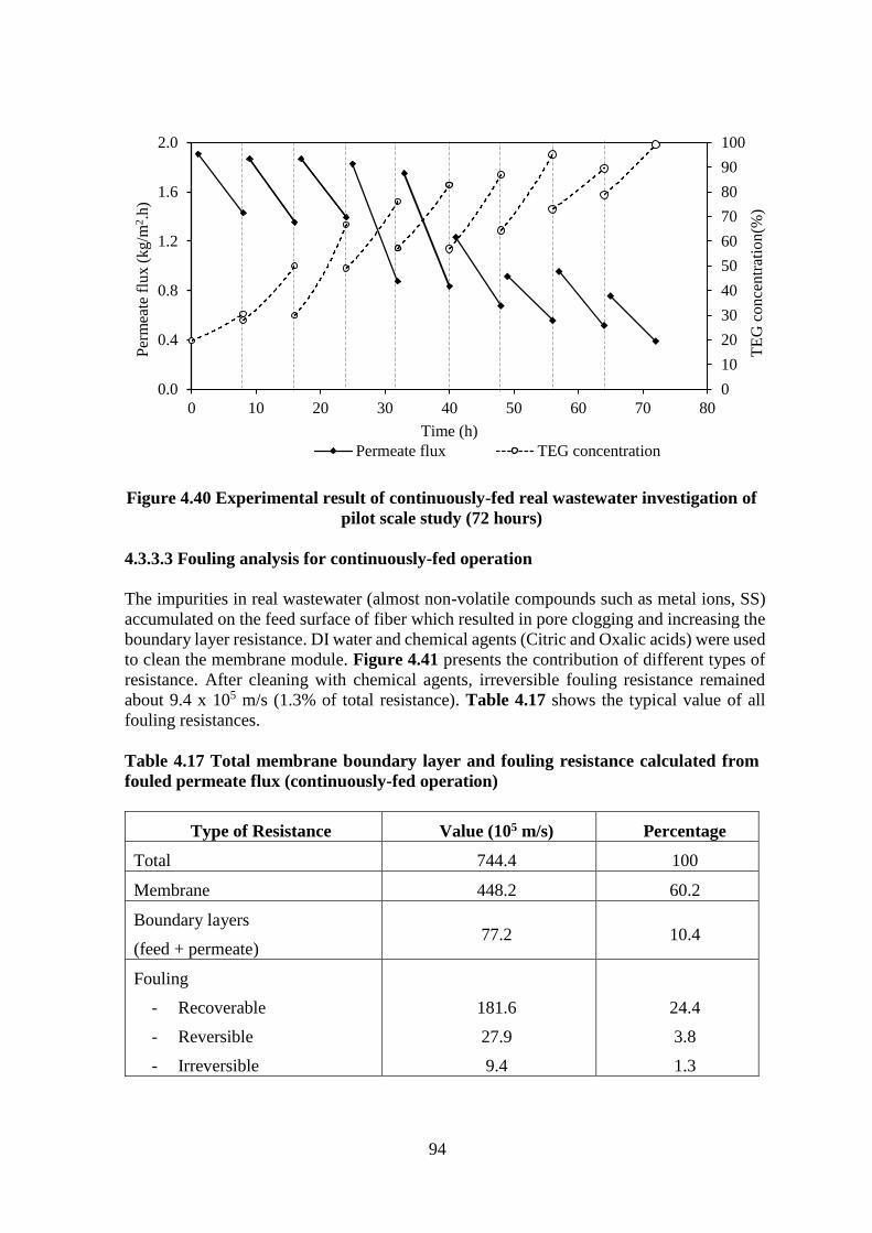
94
Figure 4.40 Experimental result of continuously-fed real wastewater investigation of
pilot scale study (72 hours)
4.3.3.3 Fouling analysis for continuously-fed operation
The impurities in real wastewater (almost non-volatile compounds such as metal ions, SS)
accumulated on the feed surface of fiber which resulted in pore clogging and increasing the
boundary layer resistance. DI water and chemical agents (Citric and Oxalic acids) were used
to clean the membrane module. Figure 4.41 presents the contribution of different types of
resistance. After cleaning with chemical agents, irreversible fouling resistance remained
about 9.4 x 10⁵ m/s (1.3% of total resistance). Table 4.17 shows the typical value of all
fouling resistances.
Table 4.17 Total membrane boundary layer and fouling resistance calculated from
fouled permeate flux (continuously-fed operation)
Type of Resistance Value (105 m/s) Percentage
Total 744.4 100
Membrane 448.2 60.2
Boundary layers
(feed + permeate) 77.2 10.4
Fouling
- Recoverable
- Reversible
- Irreversible
181.6
27.9
9.4
24.4
3.8
1.3
0
10
20
30
40
50
60
70
80
90
100
0.0
0.4
0.8
1.2
1.6
2.0
0 10 20 30 40 50 60 70 80
TE
G c
on
cen
trat
ion
(%)
Per
mea
te f
lux
(kg/m
2.h
)
Time (h)
Permeate flux TEG concentration

95
Figure 4.41 Classification of Resistances in SGMD Continuously-fed Real
Wastewater of Pilot Scale Study
Table 4.18 shows the comparison of resistance between batch and continuously-fed
experiment of pilot scale MD module. Due to the increasing of TEG concentration and
impurities, total resistance in continuously-fed experiment (744.4 x 10⁵ m/s) was higher than
that value in batch experiment (544.7 x 10⁵ m/s). During concentrating continuously,
impurities in real wastewater attached on the membrane surface without removing. Thus,
fouling resistance in continuously-fed experiment was more serious than batch experiment.
Table 4.18 Comparison of Fouling and Other Resistance between Continuously-fed
and Batch Operation
Type of Resistance Value (105 m/s)
Continuously-fed Batch
Total 744.4 544.7
Membrane 448.2 448.2
Boundary layers
(feed + permeate) 77.2 56.5
Fouling
- Recoverable
- Reversible
- Irreversible
181.6
27.9
9.4
43.4
7.3
9.4
A comparison of fouling analysis results of pilot scale MD module is presented in Table
4.19. In the research of Yuthawong (2014), MD module was investigated at the non-optimal
condition. A high total resistance (1960 x 105 m/s) resulted in low permeate flux. Boundary
layer resistance of membrane module in this situation was high (963 x 105 m/s). Moreover,
Membrane
60.2 %
Boundary layer
10.4 %
Recoverable
24.4 %
Reversible
3.8 %
Irreversible
1.3 %
Fouling
29.4 %

96
due to the unsuitable cleaning procedure (using hydrochloric acid and sodium hydroxide),
the irreversible fouling resistance (67 x 105 m/s) remained after cleaning was higher than
this study (9.4 x 10⁵ m/s). By using proper cleaning agents (citric and oxalic acid), the
irreversible fouling resistance was very less.
Table 4.19 Comparison of Fouling and Other Resistance between Normal Condition
and Optimum Condition of SGMD Hollow Fiber Membrane Distillation
(Continuously-fed)
Type of Resistance Value (105 m/s)
This study Yuthawong (2014)
Total 744.4 1960
Membrane 448.2 406
Boundary layers
(feed + permeate) 77.2 963
Fouling
- Recoverable
- Reversible
- Irreversible
181.6
27.9
9.4
501
27
67
In this study, all calculations related to feed velocity (represented by feed flow rate) used
the cross flow velocity. This velocity was determined based on the feed flow rate and cross
sectional area of the liquid flow channel. However, the local velocity at different positions
was totally different due to the sharp of module. Figure 4.42 and 4.43 show the typical
velocities profile along the module. The flow simulation were done in Solidworks software.
The characteristic of flow affected mainly on membrane surface fouling. At the area of
turbulent flow, the fouling resistance was less than that at laminar flow.
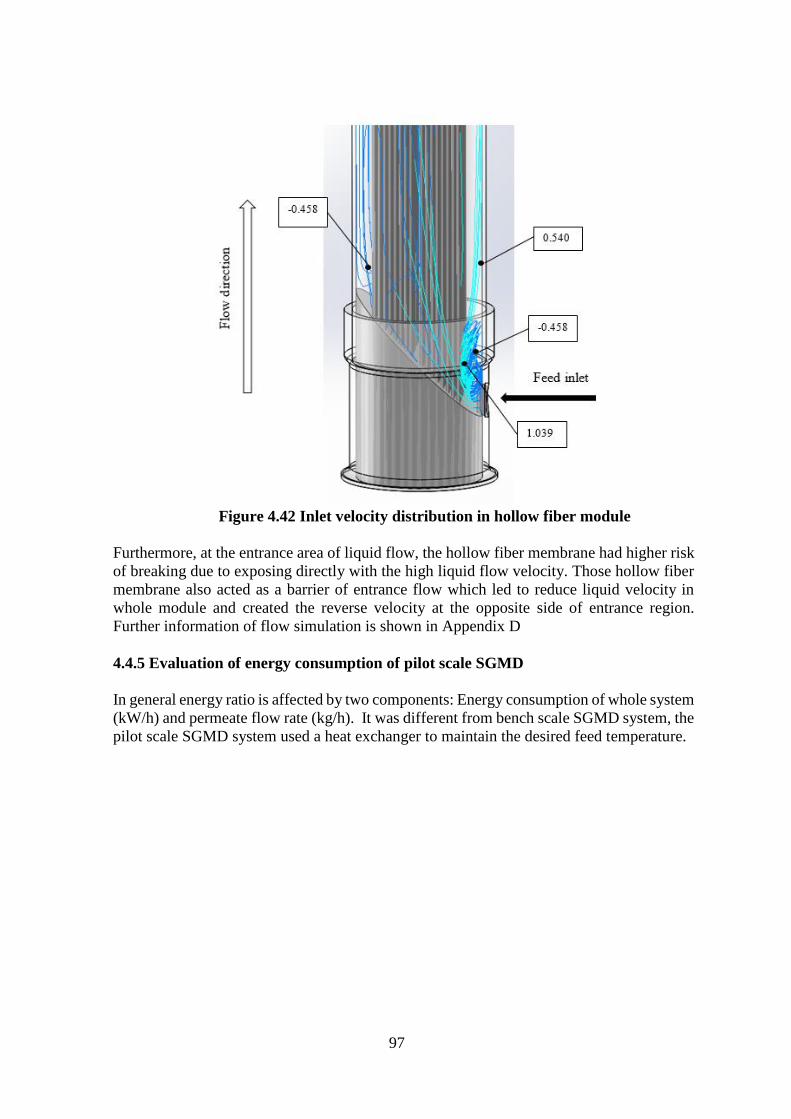
97
Figure 4.42 Inlet velocity distribution in hollow fiber module
Furthermore, at the entrance area of liquid flow, the hollow fiber membrane had higher risk
of breaking due to exposing directly with the high liquid flow velocity. Those hollow fiber
membrane also acted as a barrier of entrance flow which led to reduce liquid velocity in
whole module and created the reverse velocity at the opposite side of entrance region.
Further information of flow simulation is shown in Appendix D
4.4.5 Evaluation of energy consumption of pilot scale SGMD
In general energy ratio is affected by two components: Energy consumption of whole system
(kW/h) and permeate flow rate (kg/h). It was different from bench scale SGMD system, the
pilot scale SGMD system used a heat exchanger to maintain the desired feed temperature.
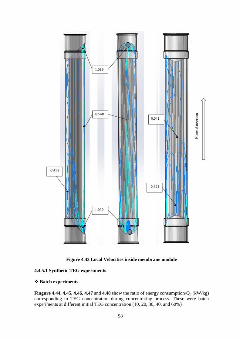
98
Figure 4.43 Local Velocities inside membrane module
4.4.5.1 Synthetic TEG experiments
Batch experiments
Fingure 4.44, 4.45, 4.46, 4.47 and 4.48 show the ratio of energy consumption/Qp (kW/kg)
corresponding to TEG concentration during concentrating process. These were batch
experiments at different initial TEG concentration (10, 20, 30, 40, and 60%)
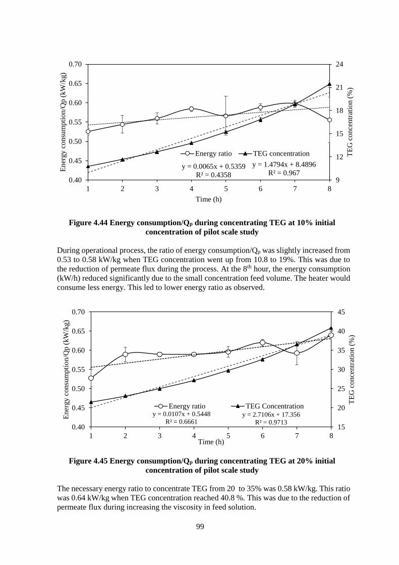
99
Figure 4.44 Energy consumption/Qp during concentrating TEG at 10% initial
concentration of pilot scale study
During operational process, the ratio of energy consumption/Qp was slightly increased from
0.53 to 0.58 kW/kg when TEG concentration went up from 10.8 to 19%. This was due to
the reduction of permeate flux during the process. At the 8th hour, the energy consumption
(kW/h) reduced significantly due to the small concentration feed volume. The heater would
consume less energy. This led to lower energy ratio as observed.
Figure 4.45 Energy consumption/Qp during concentrating TEG at 20% initial
concentration of pilot scale study
The necessary energy ratio to concentrate TEG from 20 to 35% was 0.58 kW/kg. This ratio
was 0.64 kW/kg when TEG concentration reached 40.8 %. This was due to the reduction of
permeate flux during increasing the viscosity in feed solution.
y = 0.0065x + 0.5359
R² = 0.4358
y = 1.4794x + 8.4896
R² = 0.9679
12
15
18
21
24
0.40
0.45
0.50
0.55
0.60
0.65
0.70
1 2 3 4 5 6 7 8
TE
G c
on
cen
trat
ion
(%
)
Ener
gy c
onsu
mpti
on/Q
p (
kW
/kg)
Time (h)
Energy ratio TEG concentration
y = 0.0107x + 0.5448
R² = 0.6661y = 2.7106x + 17.356
R² = 0.971315
20
25
30
35
40
45
0.40
0.45
0.50
0.55
0.60
0.65
0.70
1 2 3 4 5 6 7 8
TE
G c
once
ntr
atio
n (
%)
En
ergy c
onsu
mpti
on/Q
p (
kW
/kg)
Time (h)
Energy ratio TEG Concentration

100
Figure 4.46 Energy consumption/Qp during concentrating TEG at 30% initial
concentration of pilot scale study
Similar to the previous batch (20% initial TEG concentration), the necessary energy ratio
was 0.58 kW/kg when TEG concentration increased from 30 to 35%. The trend of energy
ratio kept on increasing after that. To concentrate TEG from 35 to 50%, the average energy
ratio required was 0.63%.
Figure 4.47 Energy consumption/Qp during concentrating TEG at 40% initial
concentration of pilot scale study
y = 0.0135x + 0.5598
R² = 0.8177
y = 3.6805x + 26.666
R² = 0.977430
35
40
45
50
55
60
0.40
0.45
0.50
0.55
0.60
0.65
0.70
1 2 3 4 5 6 7 8
TE
G c
on
cen
trat
ion
(%
)
En
ergy c
on
sum
pti
on
/Qp
(kW
/kg)
Time (h)
Energy ratio TEG Concentration
y = 0.016x + 0.6052
R² = 0.8941y = 4.0748x + 36.899
R² = 0.985335
45
55
65
75
0.50
0.55
0.60
0.65
0.70
0.75
0.80
1 2 3 4 5 6 7 8
TE
G c
once
ntr
atio
n (
%)
En
ergy c
onsu
mpti
on/Q
p (
kW
/kg)
Time (h)
Energy ratio TEG Concentration
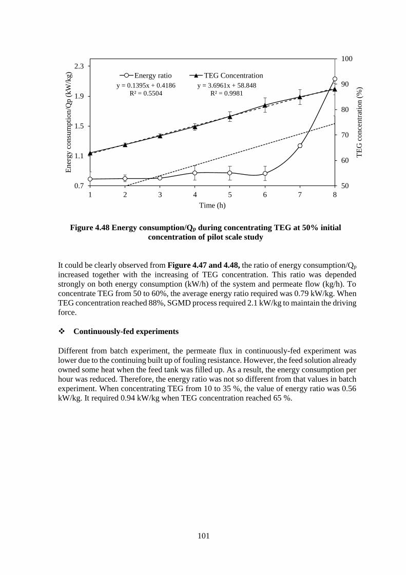
101
Figure 4.48 Energy consumption/Qp during concentrating TEG at 50% initial
concentration of pilot scale study
It could be clearly observed from Figure 4.47 and 4.48, the ratio of energy consumption/Qp
increased together with the increasing of TEG concentration. This ratio was depended
strongly on both energy consumption (kW/h) of the system and permeate flow (kg/h). To
concentrate TEG from 50 to 60%, the average energy ratio required was 0.79 kW/kg. When
TEG concentration reached 88%, SGMD process required 2.1 kW/kg to maintain the driving
force.
Continuously-fed experiments
Different from batch experiment, the permeate flux in continuously-fed experiment was
lower due to the continuing built up of fouling resistance. However, the feed solution already
owned some heat when the feed tank was filled up. As a result, the energy consumption per
hour was reduced. Therefore, the energy ratio was not so different from that values in batch
experiment. When concentrating TEG from 10 to 35 %, the value of energy ratio was 0.56
kW/kg. It required 0.94 kW/kg when TEG concentration reached 65 %.
y = 0.1395x + 0.4186
R² = 0.5504
y = 3.6961x + 58.848
R² = 0.9981
50
60
70
80
90
100
0.7
1.1
1.5
1.9
2.3
1 2 3 4 5 6 7 8
TE
G c
on
cen
trat
ion
(%
)
En
ergy c
on
sum
pti
on
/Qp
(kW
/kg)
Time (h)
Energy ratio TEG Concentration

102
Figure 4.49 Energy consumption/Qp during concentrating TEG for 40 hours of pilot
scale study
4.4.5.2 Real wastewater experiment
Batch experiments
Figure 4.50 presents the ratio of energy consumption/ permeate flow between pure water,
synthetic TEG and real waste water. In pure water test, the flux achieved was higher than
in synthetic and real wastewater. Therefore, the average energy ratio of pure water test
(within 8 hours) was 0.51 kW/kg while that value were 0.54 and 0.57 kW/kg for real
wastewater and synthetic TEG respectively.
Figure 4.50 Energy consumption/Qp of batch experiment with real wastewater of
pilot scale study
5
15
25
35
45
55
65
75
0.4
0.6
0.8
1.0
0 5 10 15 20 25 30 35 40 45
TE
G c
on
cen
trat
ion
(%)
Ener
gy c
onsu
mpti
on/Q
p (
kW
/kg)
Time (h)Energy ratio TEG concentration
4
8
12
16
20
24
0.40
0.45
0.50
0.55
0.60
0.65
0.70
1 2 3 4 5 6 7 8
TE
G co
nce
ntr
atio
n (
%)
En
ergy c
on
sum
pti
on
/Qp (
kW
/kg)
Time (h)
Real wastewater Synthetic 10%
Pure water TEG concentration
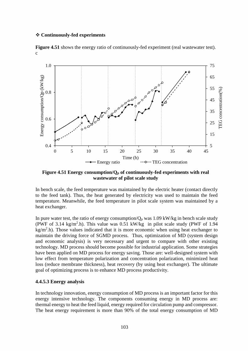
103
Continuously-fed experiments
Figure 4.51 shows the energy ratio of continuously-fed experiment (real wastewater test).
c
Figure 4.51 Energy consumption/Qp of continuously-fed experiments with real
wastewater of pilot scale study
In bench scale, the feed temperature was maintained by the electric heater (contact directly
to the feed tank). Thus, the heat generated by electricity was used to maintain the feed
temperature. Meanwhile, the feed temperature in pilot scale system was maintained by a
heat exchanger.
In pure water test, the ratio of energy consumption/Qp was 1.09 kW/kg in bench scale study
(PWF of 3.14 kg/m2.h). This value was 0.51 kW/kg in pilot scale study (PWF of 1.94
kg/m2.h). Those values indicated that it is more economic when using heat exchanger to
maintain the driving force of SGMD process. Thus, optimization of MD (system design
and economic analysis) is very necessary and urgent to compare with other existing
technology. MD process should become possible for industrial application. Some strategies
have been applied on MD process for energy saving. Those are: well-designed system with
low effect from temperature polarization and concentration polarization, minimized heat
loss (reduce membrane thickness), heat recovery (by using heat exchanger). The ultimate
goal of optimizing process is to enhance MD process productivity.
4.4.5.3 Energy analysis
In technology innovation, energy consumption of MD process is an important factor for this
energy intensive technology. The components consuming energy in MD process are:
thermal energy to heat the feed liquid, energy required for circulation pump and compressor.
The heat energy requirement is more than 90% of the total energy consumption of MD
5
15
25
35
45
55
65
75
0.4
0.6
0.8
1.0
0 5 10 15 20 25 30 35 40 45
TE
G c
on
cen
trat
ion
(%)
En
ergy c
on
sum
pti
on
/Qp
(kW
/kg)
Time (h)Energy ratio TEG concentration

104
process (Khayet and Matsuura, 2011). The ratio of energy consumption/Qp of MD process
at different TEG concentration of the continuously-fed experiment is presented in Figure
4.49. During concentrating TEG from 9.69 to 50 %, the value of energy consumption/Qp
was about 0.7 kW/kg. The permeate flux reduced when increasing TEG concentration. Thus,
the value of energy consumption/Qp increased during concentrating process
The thermal efficiency in SGMD is very high (93.2%) while that value for DCMD is
between 50-80% (Khayet and Matsuura, 2011). Thus, it can be concluded that the heat loss
is not significant in MD process. The average energy required to concentrate TEG in real
wastewater from 10 to 60 % is 0.624 kW/kg (624 kW/m3). In literature energy consumption
was evaluated for DCMD and VMD at lab scale (Criscuoli et al., 2008). The authors
conducted a study on plate-and- frame membrane module (membrane area of 40 cm2). The
lowest ratio of energy consumption/Qp obtained were 3546.3 kW/m3 and 1108.4 kW/m3 in
DCMD and VMD respectively. The performance of VMD was proven to be better than
DCMD (based on permeate flux, energy consumption and thermal efficiency). As yet,
almost studies were done theoretical modeling. Thus, it is very important to conduct study
on realistic energy consumption. Additional information about heat balances are provided
in Appendix D
4.5 Full Scale SGMD Plant Design
Based on the results of this study, a full scale SGMD system was designed for application
at the Gas Separation Plant. The main desired design criteria for full scale SGMD plant was
to concentrate 1 m3 to 0.2 m3 per day (TEG concentration increased from 10% to 50%). All
the costs (investment, operation and maintenance) was estimated based on the market price
at the designing stage. Operational condition was the optimum conditions from this study.
The details of calculations and CAD drawings are provided in Appendix B
4.5.1 Overall system design
Real TEG wastewater from PTT gas separation plant was characterized in order to evaluate
the degree of pre-treatment required prior to membrane distillation (Imdakm and Matsuura)
unit. Thus, proper pretreated wastewater was further efficiently treated by the MD process.
The result of wastewater, volatile compound and heavy metal analyzed by ALS Company
are shown in Table 4.1. A pre-treatment system is a need to keep the feed to the MD
relatively clean so that long term effective operation could be made possible. It can be noted
that suspended solids (SS) and oil and grease (O&G) have to be eliminated as they can
potentially damage membrane distillation unit. Another issue would be iron concentration
observed in sample 2 as 41 mg/L. As iron can precipitate in membrane distillation system
when the concentration of iron reaches its solubility limit as TEG concentrates in the MD
unit. However, it seemed that high iron concentration was not consistent as in sample 3, iron
concentration was very low (1.2 mg/L) and it might be due to process instability at the GSP.
The third issue that the pre-treatment system needs to address is volatile compounds which
were observed in September sample and in subsequent samplings. The volatile compounds
were benzene, toluene, ethylbenzene and xylene (BTEX). Such compounds can pass
through membrane distillation system due to their volatility and pose hazardous to the
operators. Nonetheless, both volatile compound and iron issues can be solved by adding
aeration for pre-treatment unit. Iron would potentially oxidize to precipitate during aeration
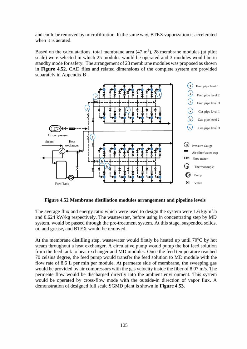
105
and could be removed by microfiltration. In the same way, BTEX vaporization is accelerated
when it is aerated.
Based on the calculatations, total membrane area (47 m2), 28 membrane modules (at pilot
scale) were selected in which 25 modules would be operated and 3 modules would be in
standby mode for safety. The arrangement of 28 membrane modules was proposed as shown
in Figure 4.52. CAD files and related dimensions of the complete system are provided
separately in Appendix B .
Figure 4.52 Membrane distillation modules arrangement and pipeline levels
The average flux and energy ratio which were used to design the system were 1.6 kg/m2.h
and 0.624 kW/kg respectively. The wastewater, before using in concentrating step by MD
system, would be passed through the pre-treatment system. At this stage, suspended solids,
oil and grease, and BTEX would be removed.
At the membrane distilling step, wastewater would firstly be heated up until 700C by hot
steam throughout a heat exchanger. A circulative pump would pump the hot feed solution
from the feed tank to heat exchanger and MD modules. Once the feed temperature reached
70 celsius degree, the feed pump would transfer the feed solution to MD module with the
flow rate of 8.6 L per min per module. At permeate side of membrane, the sweeping gas
would be provided by air compressors with the gas velocity inside the fiber of 8.07 m/s. The
permeate flow would be discharged directly into the ambient environment. This system
would be operated by cross-flow mode with the outside-in direction of vapor flux. A
demonstration of designed full scale SGMD plant is shown in Figure 4.53.
T Thermocouple
P Pressure Gauge
Pump
Valve
Flow meter
Air filter/water trap
Heat
exchanger Steam
Air compressor
Feed Tank
1
2 3
1
2
3
Feed pipe level 1
Feed pipe level 2
Feed pipe level 3
a
b
c a Gas pipe level 1
b
b Gas pipe level 2
c Gas pipe level 3

106
Figure 4.53 Sketch Diagram of Full Scale SGMD Plant

107
4.5.2 Financial analysis of full scale SGMD plant
Both investment cost and overall treatment cost of MD plant are expressed in Table 4.20. The
estimated budget information and economic analysis of full scale plant design was provided in
Appendix B.
Table 4.20 Summary of Financial Analysis for Overall System with ±30 % Variation
Components
Treatment cost
(THB)
Estimated Investment Cost
(THB)
Per year Per day Pre-treatment
system MD system
Amortization
cost 521,018 1,427
600,000 5,893,000
O &M costs 104,204 286,0
Membrane
replacement costs 716,800 1,964
Electricity cost 491,962 1,349
Labour cost 164,250 450,0
Total 1,998,234 6,083 6,493,000
*Remark:
- Assume: Plant availability is 90% (the plant operates 328 days per year)
- Treatment cost based on electricity cost, labour cost, O&M cost: 2,291 baht/m3
- In O&M cost, cleaning chemical cost was 32,400 baht per year
Due to the high price of hydrophobic MD module (about 128,000 baht/module), the investment
cost of MD system accounted for higher than 90% total investment cost. Currently, PTT is
treating TEG wastewater by incineration with the treatment cost of 4,500 baht/m3 (135,000
baht/month). Treating by MD system, the calculated treatment cost if basing only on electricity
cost, O&M cost and labour cost is 2,291 baht/m3. By concentrating from 1 m3 to 0.2 m3, the
generating wastewater per month would be 6 m3. This 6 m3 has the TEG concentration of 50%.
It can be further treated by incineration or conducting some more treatment step to reuse TEG
in dehydration process. Overall, the estimated monthly saving when using MD system prior
incineration would be 39,270 baht per month. Although the saving budget was not so high
(30% of current payment), but it would lead to open a potential to recover TEG from
wastewater since MD could be able to concentrate the real wastewater till 99%.
108
Chapter 5
Conclusions and Recommendations
This study mainly focused on optimizing the operational condition of membrane distillation
process for concentrating TEG from wastewater. Two scale of hollow fiber MD were
investigated (0.25 m2 and 2.0 m2). Each membrane module was tested with three solutions:
pure water, synthetic TEG and real wastewater alternately. The best possible condition found
from bench scale study was applied in pilot scale study. Energy consumption analysis in all
experiments was evaluated in term of the ratio of energy consumption/permeate flow. Fouling
analysis was conducted to evaluate the quality of cleaning process. All experimental results
were considered to design a full scale SGMD plant with the capacity of 1 m3/day.
5.1 Conclusions
5.1.1 Pre-treatment system
Pre-treatment unit was designed to remove suspended solids and oil and grease which may
cause operational problem such as membrane fouling and damaged membrane. Suspended
solids was removed by microfiltration (MF). Oil and grease was removed by ultrafiltration The
overall removal efficiency of the pre-treatment unit is 95% and 66% for suspended solids in
term of turbidity and oil and grease respectively. Therefore, the pre-treatment unit concluded
to efficiently remove suspended solids and oil and grease which were the targeted impurities in
real TEG wastewater.
5.1.2 Bench scale hollow fiber membrane distillation study
5.1.1.1 System verification
The optimum condition in terms of energy consumption/Qp and permeate flux were achieved
at feed flow rate of 2.4 (L/min), feed temperature of 70oC, and sweeping gas velocity of 4.7 m/s
(gas inlet flow rate of 0.255 L/min.fiber). At this condition, pure water flux achieved was 3.14
kg/m2.h, the ratio of energy consumption/Qp was 1.09 kWh/kg. The bench scale MD module
has ability to reject 99.99 % of non-volatile substance.
5.1.2.2 Synthetic TEG investigation
The hollow fiber MD was tested at 10% initial TEG concentration. During concentrating TEG
from 10 to 45 %, the permeate flux was in the range from 2.61 to 2.1 kg/m2.h with the ratio of
energy consumption/Qp was approximately 1.29 kW/kg.
The boundary layer resistance of SGMD was not considered as a serious problem. It contributes
only about 10-20% of total resistance and can be removed by rising the system with DI water.
Bench scale MD module has ability to concentrate synthetic TEG till 90%

109
5.1.2.3 Real wastewater investigation
The permeate flux of real wastewater investigation when concentrating TEG from 9.69 to 50%
were in the range from 2.4 to 1.6 kg/m2.h with the ratio of energy consumption/Qp was 1.4
kWh/kg.It could concentrate TEG in real wastewater till 98.01%.
In the total resistance, membrane resistance, boundary layer resistance, fouling resistance
contributed 69.2 %, 7.6%, 23.2 % respectively. The irreversible resistance accounted for 2%.
5.1.3 Pilot scale hollow fiber membrane distillation study
5.1.3.1 System verification
The optimum condition was decided at the gas velocity of 8.07 m/s (gas inlet flow rate of 0.44
L/min.fiber), feed inlet temperature of 70oC. Feed flow rate and sweeping gas temperature have
less effect. The flux achieved was 1.94 kg/m2.h. At this condition, the ratio of energy
consumption/Qp was 0.51 kW/kg.
Synthetic TEG 10% was used as the feed solution to conduct the rejection test. The pilot scale
MD module could reject 99.99 % of non-volatile material.
5.1.3.2 Synthetic TEG investigation
Synthetic TEG (10%) was used as the feed solution. The permeate flux was stable around 1.8
kg/m2.h when the TEG concentration was less than 30 %. When the TEG concentration was in
the range from 30% to 50%, permeate flux was about 1.6 kg/m2.h (average). At higher TEG
concentration (>50%), the flux reduced to less than 1.2 kg/m2.h.
When TEG concentration was in the range from 10 to 60%, the ratio of energy consumption/Qp
was less than 0.7 kW/kg.
Pilot scale MD module has ability to concentrate synthetic TEG till 98.7%
During increasing of TEG concentration (from 10 to 80%), the boundary layer resistance
increased from 51.8 to 133 x 105 m/s. Its contribution to the total resistance increased from 10.4
% to 22.5% which was the main reason of reduction of permeate flux.
5.1.3.3 Real wastewater investigation
The permeate flux was higher than 1.7 kg/m2.h with the TEG concentration less than 15 %. The
flux reduced to the range between 1.4 and 1.65 kg/m2.h at higher TEG concentration from the
hour of 5th and 28th (TEG concentration less than 50%). It reached 0.9 kg/m2.h at the hour of
40th (final TEG concentration was about 69.4 %)
Pilot scale SGMD module has ability to concentrate TEG in real wastewater until 99.1%
110
The contributions of membrane resistance, boundary layer resistance and fouling resistance into
the total resistance were 60.2 %, 10.4 % and 29.4% respectively. After cleaning with chemical
agents, irreversible fouling resistance remained 1.3% total resistance.
To concentrate real wastewater from 10 to 45 % TEG concentration, the required energy ratio
was 0.62 kW/kg. The energy ratio in real wastewater and synthetic TEG were similar at 0.95
kW/kg when concentrating TEG continuously up to 65%.
5.2 Recommendations for Future Study
Membrane distillation is a new technology. Commercialization has not been applied for MD
technology yet. Thus, some recommendations for further research are proposed as followings:
1. The liquid entry pressure (LEP) should be put more intention when using hydrophobic
membrane distillation. This factor helps to ensure that the system is working well with
membrane distillation process. Especially, the relationship between membrane (material,
pore size, thickness, hydrophobicity) and operational condition (feed flow rate, sweeping
gas velocity, temperature, concentration) should be studied deeply.
2. The wastewater discharged from textile industry is becoming a big environmental issue.
Hot textile wastewater is fully infested by dye materials. In textile industry, dyeing step
creates the highest risk for environment (organic dyes, additives and salts). Dyes almost
are non-volatile compounds (mono- and poly- azo). Since the principle of membrane
distillation process is based on the different in vapor pressure between feed side and
permeate side, it is a great potential to recover valuable materials from hot dyeing solution.
Further study should focus on practicalization of recovering dye compounds (i.e.
methylene blue-C16H18ClN3S.3H2O) from synthetic dyeing wastewater. Membrane
distillation can be used to concentrate dyes according to the temperature of dye bath
solution (usually 80-90oC) ,
3. Membrane distillation hybrid system: since it is not necessary to heat the feed solution till
boiling point of its material, the combination between membrane distillation system
(especially heating step) and solar energy system should be studied in depth. According
to the state of art of membrane distillation technology, energy consumption has become
a vital factor that make it become comparable to other conventional process (i.e. RO, MF,
UF). However, there is potential to reduce energy consumption by using solar energy (free
natural energy source).
4. The best available cleaning method for hydrophobic membrane distillation has not been
studied sufficiently. This includes chemical agents, concentration and procedure. It is a
demand for this technology on protect the hydrophobicity of membrane. Further studies
should clarify the interaction between chemical agents and hydrophobic characteristic.
The changes of water contact angle on membrane surface after conducting cleaning step
should be clarified.
111
5. Extensive study should be conducted to understand the effect of the fiber length in SGMD
process. The shorter hollow fiber might lead to better MD performance (in terms of both
concentrating efficiency and energy consumption). Moreover, the effect of hollow fiber’s
thickness should also be studied sufficiently. The membrane thickness has significant
effect on heat loss during membrane distillation process.
112
Reference
Alberta-Environment (2010). Soil and groundwater remediation guidelines for diethlyene
glycol and triethylene glycol. Retrieved from http://www.environment.alberta.ca/0
3284.html
Alkhudhiri, A., Darwish, N., and Hilal, N. (2012). Membrane distillation: A comprehensive
review. Desalination, 287(0), 2-18.
Andrjesdóttir, Ó., Ong, C. L., Nabavi, M., Paredes, S., Khalil, A. S. G., Michel, B., and
Poulikakos, D. (2013). An experimentally optimized model for heat and mass transfer
in direct contact membrane distillation. International Journal of Heat and Mass
Transfer, 66(0), 855-867.
Banat, F. A., and Simandl, J. (1994). Theoretical and experimental study in membrane
distillation. Desalination, 95(1), 39-52.
Bandini, S., Gostoli, C., and Sarti, G. C. (1992). Separation efficiency in vacuum membrane
distillation. Journal of Membrane Science, 73(2–3), 217-229.
Criscuoli, A., Carnevale, M. C., and Drioli, E. (2008). Evaluation of energy requirements in
membrane distillation. Chemical Engineering and Processing: Process Intensification,
47(7), 1098-1105.
Daigger and Crawford. (2005). Incorporation of Biological Nutrient Removal (BNR) Into
Membrane Bioreactors (MBRs). Paper presented at the Proceedings of the IWA
Specialized Conference, Nutrient Management in Wastewater Treatment Processes
and Recycle Streams, Krakow Poland
Daigger, T, G., Lozier, C, J., and Crawford, V., e. (2006). Water Reuse Applications Using
Membrane Technology. Paper presented at the Water Environment Federation.
Ding, Z., Liu, L., Li, Z., Ma, R., and Yang, Z. (2006). Experimental study of ammonia removal
from water by membrane distillation (MD): The comparison of three configurations.
Journal of Membrane Science, 286(1–2), 93-103.
Dow. (2014). Triethylen Glycol. Retrieved on 24th June, 2014 from http://www.dow.com/eth
yleneglycolprod/teg.htm
El-Bourawi, M. S., Ding, Z., Ma, R., and Khayet, M. (2006). A framework for better
understanding membrane distillation separation process. Journal of Membrane
Science, 285(1–2), 4-29.
113
Fujii, Y., Kigoshi, S., Iwatani, H., Aoyama, M., and Fusaoka, Y. (1992). Selectivity and
characteristics of direct contact membrane distillation type experiment. II. Membrane
treatment and selectivity increase. Journal of Membrane Science, 72(1), 73-89.
Garcı́a-Payo, M. C., Izquierdo-Gil, M. A., and Fernández-Pineda, C. (2000). Air gap
membrane distillation of aqueous alcohol solutions. Journal of Membrane Science,
169(1), 61-80.
Guillen-Burrieza, E., Ruiz-Aguirre, A., Zaragoza, G., and Arafat, H. A. (2014). Membrane
fouling and cleaning in long term plant-scale membrane distillation operations. Journal
of Membrane Science, 468 (0), 360-372.
Ibrahim, N. K. (2010). Gas Technology Lectures. Retrieved on 15th July, 2014 from
http://www.lopdf.net/preview/Hev1_7mP_P4bgJE1QrfCFBWSzw84ie1dOeFBY5JFr
c,/Gas-Technology-Lectures.html?query=Gas-Technology-Lectures
Imdakm, A. O., and Matsuura, T. (2004). A Monte Carlo simulation model for membrane
distillation processes: direct contact (MD). Journal of Membrane Science, 237(1–2),
51-59.
Izquierdo-Gil, M. A., and Jonsson, G. (2003). Factors affecting flux and ethanol separation
performance in vacuum membrane distillation (VMD). Journal of Membrane Science,
214(1), 113-130.
Jacob, P., Rattanaoudom, R., Khachonbuna, P., Piyaprachakorn, N., Thummadetsak, G., and
Visvanathan, C. (2014). Potential Membrane Based Treatment of Triethylene Glycol
Wastewater from Gas Separation Plant Journal of Water Sustainability, 4(2), 123-136.
Jehle, W., Staneff, T., Wagner, B. and Steinwandel, J. (1995). Separation of glycol and water
from coolant liquids by evaporation, reverse osmosis and pervaporation. Journal of
Membrane Science, 102(1), 9-19.
Khayet, M. (2011). Membranes and theoretical modeling of membrane distillation: A review.
Advances in Colloid and Interface Science, 164(1–2), 56-88.
Khayet, M., Cojocaru, C., and Baroudi, A. (2012). Modeling and optimization of sweeping gas
membrane distillation. Desalination, 287(0), 159-166.
Khayet, M., Godino, P., and Mengual, J. I. (2004). Study of asymmetric polarization in direct
contact membrane distillation. Separation Science and Technology, 39(1), 125-147.
Khayet, M., Godino, P., and Mengual, J. I. (2000). Theory and experiments on sweeping gas
membrane distillation. Journal of Membrane Science, 165(2), 261-272.
Khayet, M., Godino, P.,, and Mengual, J. I. (2002). Thermal boundary layers in sweeping gas
membrane distillation processes. AIChE Journal, 48 (7), 1488–1497. d

114
Khayet, M., and Matsuura, T. (2011). Membrane Distillation Principles and Applications
(1st edition). Amsterdam: Elsevier. ISBN: 978-0-444-53126-1
Khayet, M., Mengual, J. I., and Matsuura, T. (2005). Porous hydrophobic/hydrophilic
composite membranes: Application in desalination using direct contact membrane
distillation. Journal of Membrane Science, 252(1–2), 101-113.
Laganà, F., Barbieri, G., and Drioli, E. (2000). Direct contact membrane distillation: modelling
and concentration experiments. Journal of Membrane Science, 166(1), 1-11.
Larpkiattaworn, S., Eamchotchawalit, C., Pannoi, J., Keawsupsak, K., Rattanaudom, R., and
Bajpai, P. (2013). PES Membrane Performance for Triethylene Glycol (TEG)
Removal of Wastewater from Natural Gas Separation Process. Jurnal Teknologi,
65(4), 29–32.
Lawson, K. W., and Lloyd, D. R. (1997). Membrane distillation. Journal of Membrane
Science, 124(1), 1-25.
Lee, C. H., and Hong, W. H. (2001). Effect of operating variables on the flux and selectivity
in sweep gas membrane distillation for dilute aqueous isopropanol. Journal of
Membrane Science, 188(1), 79-86.
Li, J.-M., Xu, Z.-K., Liu, Z.-M., Yuan, W.-F., Xiang, H., Wang, S.-Y., and Xu, Y.-Y. (2003).
Microporous polypropylene and polyethylene hollow fiber membranes. Part 3.
Experimental studies on membrane distillation for desalination. Desalination, 155(2),
153-156.
Liu, C., Rainwater, K., and Song, L. (2011). Energy analysis and efficiency assessment of
reverse osmosis desalination process. Desalination, 276(1–3), 352-358.
Macedonio, F., Curcio, E., and Drioli, E. (2007). Integrated membrane systems for seawater
desalination: energetic and exergetic analysis, economic evaluation, experimental
study. Desalination, 203(1–3), 260-276.
Martı́nez, L., Florido-Dı́az, F. J., Hernández, A., and Prádanos, P. (2003). Estimation of vapor
transfer coefficient of hydrophobic porous membranes for applications in membrane
distillation. Separation and Purification Technology, 33(1), 45-55.
Meindersma, G. W., Guijt, C. M., and De Haan, A. B. (2006). Desalination and water recycling
by air gap membrane distillation. Desalination, 187(1–3), 291-301.
Metcaf and Eddy. (2003). Wastewater Engineering-Treatment and reuse (4th edition). New
York: Mc Graw-Hill.
Mokhatab, S., Poe, W. A., and Speight, J. G. (2006). Handbook of Natural Gas Transmission
and Processing (1st edition). United states: Gulf Professional Publishing.

115
Orecki, A., Tomaszewska, M., Karakulski, K. and Morawski, A.W. (2006). Separation of
ethylene glycol from model wastewater by nanofiltration. Desalination, 200(1), 358-
360
Padaki, M., Surya Murali, R., Abdullah, M. S., Misdan, N., Moslehyani, A., Kassim, M. A.,
and Ismail, A. F. (2015). Membrane technology enhancement in oil–water separation.
A review. Desalination, 357(0), 197-207.
Phattaranawik, J., and Jiraratananon, R. (2001). Direct contact membrane distillation: effect of
mass transfer on heat transfer. Journal of Membrane Science, 188(1), 137-143.
Phattaranawik, J., Jiraratananon, R., and Fane, A. G. (2003). Heat transport and membrane
distillation coefficients in direct contact membrane distillation. Journal of Membrane
Science, 212(1–2), 177-193.
PTT-GSP. (2012). TEG Wastewater characterisitcs. In P. Research (Edition). 1st meeting on
TEG wastewater Treatment in Gas Separation Plant at PTT Gas Separation Plant,
Rayong, Thailand PTT Gas Separation Plant, Thailand.
Qtaishat, M., Matsuura, T., Kruczek, B., and Khayet, M. (2008). Heat and mass transfer
analysis in direct contact membrane distillation. Desalination, 219(1–3), 272-292.
Sakai, K., Koyano, T., Muroi, T., and Tamura, M. (1988). Effects of temperature and
concentration polarization on water vapour permeability for blood in membrane
distillation. The Chemical Engineering Journal, 38(3), B33-B39.
Sarbatly, R., and Chiam, C.-K. (2013). Evaluation of geothermal energy in desalination by
vacuum membrane distillation. Applied Energy, 112(0), 737-746.
Schofield, R. W., Fane, A. G., and Fell, C. J. D. (1990). Gas and vapour transport through
microporous membranes. II. Membrane distillation. Journal of Membrane Science,
53(1–2), 173-185.
Smolders, K., and Franken, A. C. M. (1989). Terminology for Membrane Distillation.
Desalination, 72(3), 249-262.
Srisurichan, S., Jiraratananon, R., and Fane, A. G. (2005). Humic acid fouling in the membrane
distillation process. Desalination, 174(1), 63-72.
Sun, A. C., Kosar, W., Zhang, Y., and Feng, X. (2014). Vacuum membrane distillation for
desalination of water using hollow fiber membranes. Journal of Membrane Science,
455(0), 131-142.
Susanto, H. (2011). Towards practical implementations of membrane distillation. Chemical
Engineering and Processing: Process Intensification, 50(2), 139-150.
116
Thanh, B. X., and Dan, N. P. (2013). Study on treatment performance of low cost membrane
based septic tank at various fluxes. Internat. J. Waste Resources, 3(1), 1-4.
Tomaszewska, M., Gryta, M., and Morawski, A. W. (1998). The influence of salt in solutions
on hydrochloric acid recovery by membrane distillation. Separation and Purification
Technology, 14(1–3), 183-188.
Tun, C. M., Fane, A. G., Matheickal, J. T., and Sheikholeslami, R. (2005). Membrane
distillation crystallization of concentrated salts—flux and crystal formation. Journal of
Membrane Science, 257(1–2), 144-155.
Vincenza Calabro , B. L. J., and Enrico Drioli. (1994). Theoretical and Experimental Study on
Membrane Distillation in the Concentration of Orange Juice. Ind. Eng. Chem. Res.,
33(7), 1803–1808.
Xie, Z. , Duong, T. , Hoang, M. , Nguyen, C. and Bolto, B. (2009). Ammonia removal by
sweep gas membrane distillation. Water Research, 43(6), 1693-1699.
Yang, X., Yu, H., Wang, R., and Fane, A. G. (2012). Analysis of the effect of turbulence
promoters in hollow fiber membrane distillation modules by computational fluid
dynamic (CFD) simulations. Journal of Membrane Science, 415–416(0), 758-769.
Yuthawong, V. (2014). Pilot scale study on separation of triethylene glycol from gas
separation plant wastestream using membrane distillation process. (Master Thesis No.
EV-14-13. Asian Institute of Technology, 2014). Bangkok: Asian Institute of
Technology.
Zhang, S. Q., Kumar, A., and Kutowy, O. (2000). Membrane-based separation scheme for
processing sweeteners from stevia leaves. Food Research International, 33(7), 617-
620.
Zhao, S. , Feron, P. H. M. , Xie, Z. , Zhang, J. and Hoang, M. (2014). Condensation studies in
membrane evaporation and sweeping gas membrane distillation. Journal of Membrane
Science, 462(0), 9-16.
Zuo, G., Wang, R., Field, R., and Fane, A. G. (2011). Energy efficiency evaluation and
economic analyses of direct contact membrane distillation system using Aspen Plus.
Desalination, 283(0), 237-244.
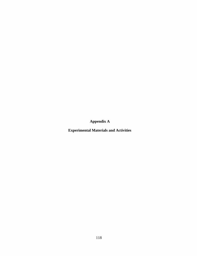
118
Appendix A
Experimental Materials and Activities
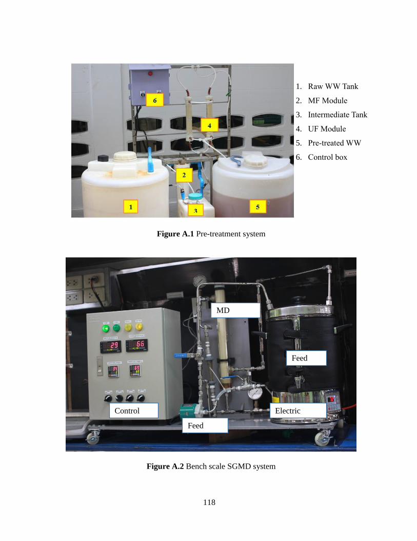
118
Figure A.1 Pre-treatment system
Figure A.2 Bench scale SGMD system
Feed
tank
Electric
heater Feed
pump
Control
box
MD
module
1. Raw WW Tank
2. MF Module
3. Intermediate Tank
4. UF Module
5. Pre-treated WW
6. Control box
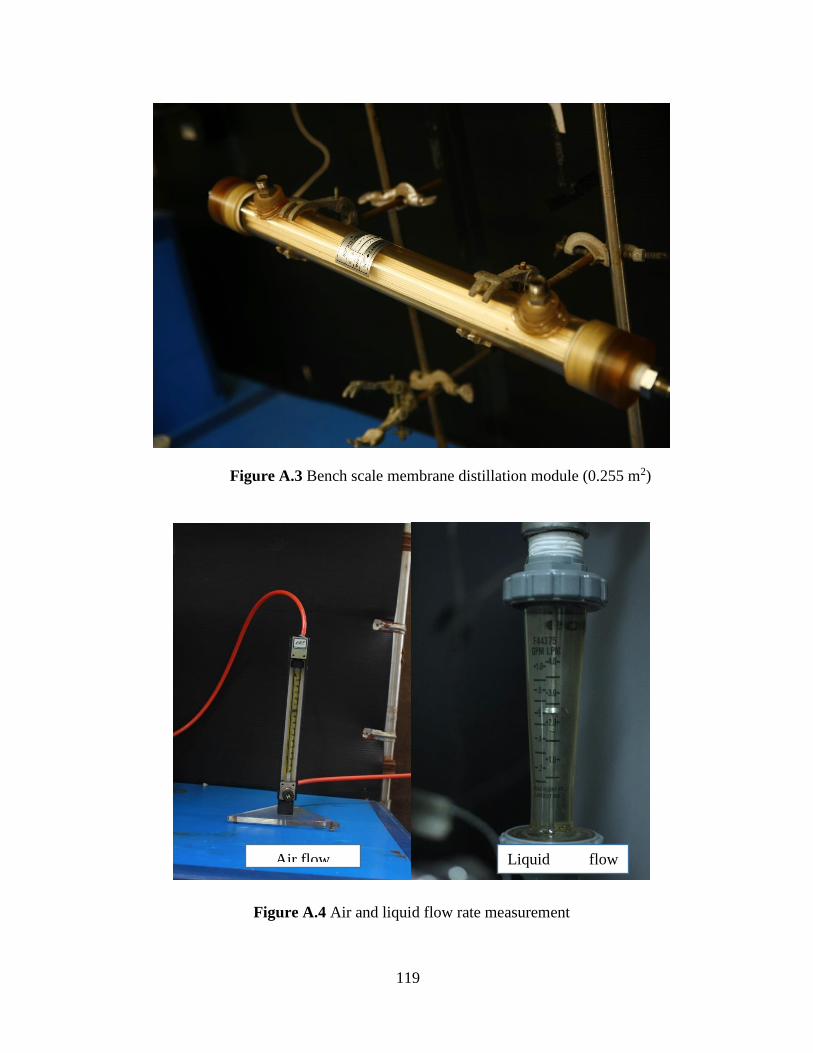
119
Figure A.3 Bench scale membrane distillation module (0.255 m2)
Figure A.4 Air and liquid flow rate measurement
Air flow
meter
Liquid flow
meter
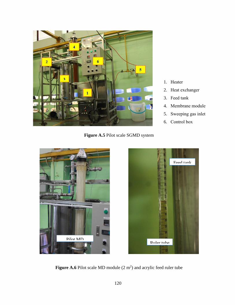
120
Figure A.5 Pilot scale SGMD system
Figure A.6 Pilot scale MD module (2 m2) and acrylic feed ruler tube
1. Heater
2. Heat exchanger
3. Feed tank
4. Membrane module
5. Sweeping gas inlet
6. Control box
Pilot MD
module Ruler tube
Feed tank

121
Figure A.7 Energy consumption measurement
Figure A.8 Water condensed at the outlet of membrane module

122
Figure A.9 Student operating and maintaining the system
123
Appendix B
Full Scale Sweeping Gas Membrane Distillation Plant Design
Calculations and Drawings
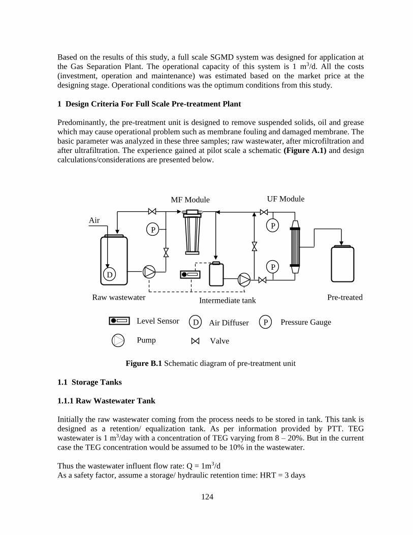
124
Based on the results of this study, a full scale SGMD system was designed for application at
the Gas Separation Plant. The operational capacity of this system is 1 m3/d. All the costs
(investment, operation and maintenance) was estimated based on the market price at the
designing stage. Operational conditions was the optimum conditions from this study.
1 Design Criteria For Full Scale Pre-treatment Plant
Predominantly, the pre-treatment unit is designed to remove suspended solids, oil and grease
which may cause operational problem such as membrane fouling and damaged membrane. The
basic parameter was analyzed in these three samples; raw wastewater, after microfiltration and
after ultrafiltration. The experience gained at pilot scale a schematic (Figure A.1) and design
calculations/considerations are presented below.
Figure B.1 Schematic diagram of pre-treatment unit
1.1 Storage Tanks
1.1.1 Raw Wastewater Tank
Initially the raw wastewater coming from the process needs to be stored in tank. This tank is
designed as a retention/ equalization tank. As per information provided by PTT. TEG
wastewater is 1 m3/day with a concentration of TEG varying from 8 – 20%. But in the current
case the TEG concentration would be assumed to be 10% in the wastewater.
Thus the wastewater influent flow rate: Q = 1m3/d
As a safety factor, assume a storage/ hydraulic retention time: HRT = 3 days
Raw wastewater
tank
D
Intermediate tank Pre-treated
tank
UF Module MF Module
P
Air
P P
Level Sensor D Air Diffuser P Pressure Gauge
Pump Valve

125
Thus the required volume of the tank would be (V) =5 m3
The readily available product with this requirement is presented below with the image as figure
B.3
Choose
Company: Mixer Direct, Inc.
Dimensions (mm): a = 1000, b = 200, c = 4000 , d = 200 , e = 420, f = 63.5, g = 40, h = 40
Inside diameter: 960 mm
Thickness: 20 mm
Nominal capacity: 3250 L
Material: Stainless steel
Figure B.2 TEG Wastewater Tank (custom design)
1.1.2 Intermediate Tank
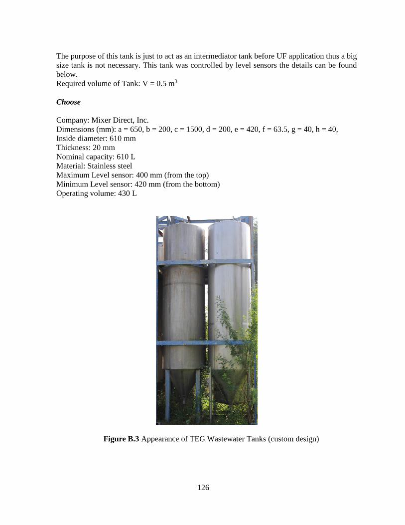
126
The purpose of this tank is just to act as an intermediator tank before UF application thus a big
size tank is not necessary. This tank was controlled by level sensors the details can be found
below.
Required volume of Tank: V = 0.5 m3
Choose
Company: Mixer Direct, Inc.
Dimensions (mm): a = 650, b = 200, c = 1500, d = 200, e = 420, f = 63.5, g = 40, h = 40,
Inside diameter: 610 mm
Thickness: 20 mm
Nominal capacity: 610 L
Material: Stainless steel
Maximum Level sensor: 400 mm (from the top)
Minimum Level sensor: 420 mm (from the bottom)
Operating volume: 430 L
Figure B.3 Appearance of TEG Wastewater Tanks (custom design)
127
1.1.3 Pre-treated Tank
Required volume of Tank: V = 1.3 m3
Choose
Compagnie: Mixer Direct, Inc.
Dimensions (mm): a = 1000, b = 200, c = 1600, d = 200 , e = 420, f = 63.5,
g = 40, h = 40,
Inside diameter: 960 mm
Thickness: 20 mm
Nominal capacity: 1366 L
Material: Stainless steel
Maximum Level sensor: 400 mm (from the top)
Minimum Level sensor: 420 mm (from the bottom)
Operating volume: 1100 L
1.2 Microfiltration and ultrafiltration module design
The overall design of the pre-treatment system would be 1 m3/d. Thus a specific membrane
module are provided based on these results.
1.2.1 MF module
The flux is determined by the properties of membrane, driving force and characteristic of the
feed.
Assume: Water recovery of MF/UF are 99% respectively
→ Permeate flow from MF is 1.01 m3/day.
Permeate flux = 150 L/m2.h, Filtration duration 8 hours per day
Permeate flow: Qp = 1.01 m3/ 8 h = 126.3 L/h
Permeate flux: 50 L/m2.h
→ Total membrane area required: A = Qp / J = 126.3 (L/h) /50 (L/m2.h) = 2.5 m2
Choose:
Company: Microdyn-Nadir (Xiamen) Co., Ltd, China
Model: MD 070 FP 2L
Membrane material: Polypropylene-Hollow fiber modules
Filtration surface Area: 2.2 m2
Membrane pore size: 0.2 µm
Hydrophobicity: Hydrophilic
Shell material: Polypropylene
Inner diameter: 0.6 mm
Module length: 1400 mm
Number of module: 2

128
1.2.2 UF module
Assume: The system was operated 8 h/day
Permeate flow: Qp = 1 m3/ 8 h = 125 L/h
Permeate flux: 40 L/m2.h
→ Total membrane area required: A = Qp / J = 125 (L/h) /40 (L/m2.h) = 3.125 m2
Choose
Company: Pall Corporation,
Model: 60P37-30
Membrane material: Ceramic
Porosity: >30%
Length: 1020 mm
Number of elements: 19
Filtration surface Area: 4.6 m2
Membrane pore size: 50 nm
Channel size: 4 mm
Hydrophobicity: Hydrophilic
Shell material: L316 Stainless steel
Gaskets material: PTFE
1.3 Pre-treatment Process Operation
1.3.1 Aeration of BTEX Removal
As BTEX concentration in the real TEG wastewater, each of the compound’s concentrations
are listed in Table B.1.
Table B.1 BTEX Concentration in 10% TEG Real Wastewater and Henry’s Law
Constant
BTEX Compound Concentration
(mg/L)
Henry’s Law Constanta at 25oC
(atm)
Benzene 26.6 306
Toluene 14.1 372
Ethylbenzene ND 486
m,p-Xylene 7.4 382b
o-Xylene 14.7 293
*Remark: ND – Not detect, a – source: Freeman (1990)
Stripping factor can be calculated by Equation below (Freeman, 1995)

129
SF = (H
Pt)(
G
L)
Where:
H = Henry’s constant (atm)
Pt = Total system pressure
G = Gas flow rate (mol/h)
L = liquid flow rate (mol/h).
Stripping factor (SF) should be in the range from 5 to 20 (Freeman, 1995). Once the removal is
completed, SF equals to 1. The higher Henry’s constant, the lower solubility in water of that
compound. Thus, o-Xylene is selected to calculate SF.
From ideal gas laws, density of air can be calculated as following:
PV = nRT →n
V= ρa =
P
RT
At 25oC, 1 atm.
ρa =1 atm
8.20578 × 10⁻² L. atmK. mol
× 298.15 K= 0.041
mol
L
Density of water:
ρw = 1000 g
L×
mol
18 g= 55.56
mol
L
From Equation 1, choose SF =5:
5 = (293 atm
1 atm) × (
G
L)
→ (G
L) = 5 × (
1atm
293 atm) ×
mol h⁄
mol h⁄×
55.56 mol L⁄
0.041 mol L⁄= 23.13 (
L h⁄
L h⁄)
Thus, At SF = 5, the air-to-water ratio is 23.13
Aeration was applied directly at the raw wastewater tank via an air diffuser.
1.3.2 Filtration Step
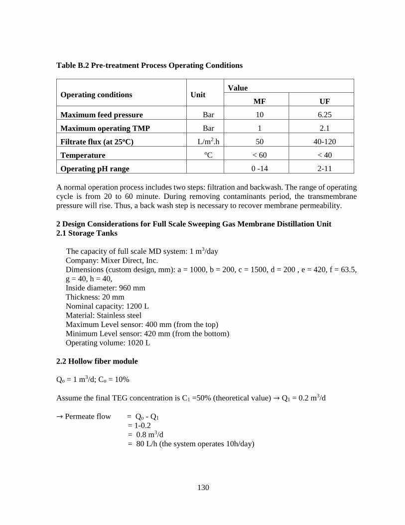
130
Table B.2 Pre-treatment Process Operating Conditions
Operating conditions Unit Value
MF UF
Maximum feed pressure Bar 10 6.25
Maximum operating TMP Bar 1 2.1
Filtrate flux (at 25oC) L/m2.h 50 40-120
Temperature oC < 60 < 40
Operating pH range 0 -14 2-11
A normal operation process includes two steps: filtration and backwash. The range of operating
cycle is from 20 to 60 minute. During removing contaminants period, the transmembrane
pressure will rise. Thus, a back wash step is necessary to recover membrane permeability.
2 Design Considerations for Full Scale Sweeping Gas Membrane Distillation Unit
2.1 Storage Tanks
The capacity of full scale MD system: 1 m3/day
Company: Mixer Direct, Inc.
Dimensions (custom design, mm): a = 1000, b = 200, c = 1500, d = 200 , e = 420, f = 63.5,
g = 40, h = 40,
Inside diameter: 960 mm
Thickness: 20 mm
Nominal capacity: 1200 L
Material: Stainless steel
Maximum Level sensor: 400 mm (from the top)
Minimum Level sensor: 420 mm (from the bottom)
Operating volume: 1020 L
2.2 Hollow fiber module
Qo = 1 m3/d; Co = 10%
Assume the final TEG concentration is C1 =50% (theoretical value) → Q1 = 0.2 m3/d
→ Permeate flow = Qo - Q1
= 1-0.2
= 0.8 m3/d
= 80 L/h (the system operates 10h/day)
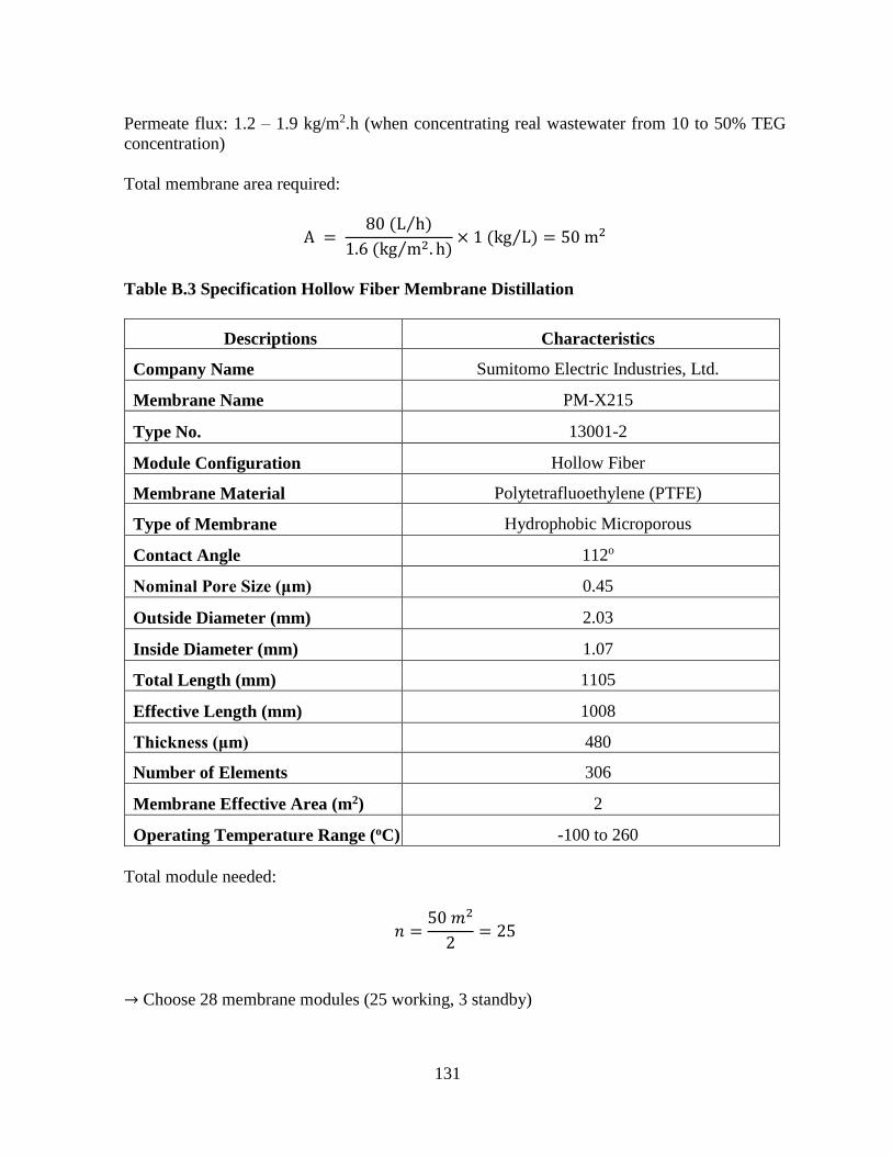
131
Permeate flux: 1.2 – 1.9 kg/m2.h (when concentrating real wastewater from 10 to 50% TEG
concentration)
Total membrane area required:
A = 80 (L h⁄ )
1.6 (kg m2. h)⁄× 1 (kg L) = 50 m2⁄
Table B.3 Specification Hollow Fiber Membrane Distillation
Descriptions Characteristics
Company Name Sumitomo Electric Industries, Ltd.
Membrane Name PM-X215
Type No. 13001-2
Module Configuration Hollow Fiber
Membrane Material Polytetrafluoethylene (PTFE)
Type of Membrane Hydrophobic Microporous
Contact Angle 112o
Nominal Pore Size (μm) 0.45
Outside Diameter (mm) 2.03
Inside Diameter (mm) 1.07
Total Length (mm) 1105
Effective Length (mm) 1008
Thickness (μm) 480
Number of Elements 306
Membrane Effective Area (m2) 2
Operating Temperature Range (oC) -100 to 260
Total module needed:
𝑛 =50 𝑚2
2= 25
→ Choose 28 membrane modules (25 working, 3 standby)

132
Table B.4 Membrane Module Specification
Description Characteristics
Type of Membrane Module Hollow Fiber
Module Configuration SGMD
Frame Material Polysulfone
Driving Force Thermal Driven
Inner Space (cm3) 7,300
Pipe Diameter (mm) 25.4 (feed)/6 (permeate)
Number of fiber 306 fibers/module
Dimension of Module (cm)
- Diameter
- Length
9.6
110.5
Operating Temperature Range
(oC) -100 to 149
pH Range 2-13
Membrane System Fabrication
Number of module: 28
CAD files and related dimensions of the complete system are provided separately.
2.3 Gas compressor
Pilot scale module: 306 fiber/module
Optimum Inlet Gas Flow rate: 133 L/min
Gas flow rate per fiber =133 L min⁄
306 fibers= 0.44 L/min
The sweeping gas flow rate needed for pilot scale module (306 fibers/module):
Qgas = 0.44 L/ min × 306 fibers × 25 modules = 3366 L/min
= 3.23 m3/min
Number of gas compressors: 3 (2 operate and 1 standby). These calculations are based on the
optimization results obtained from pilot scale testing.
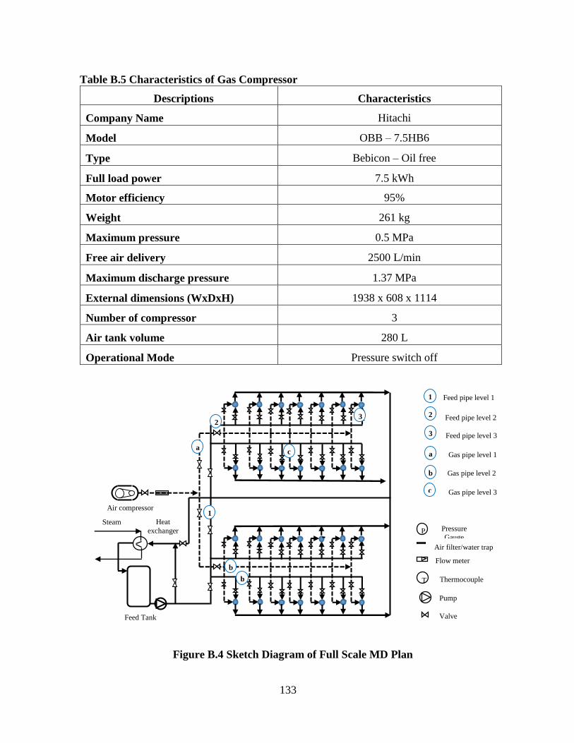
133
Table B.5 Characteristics of Gas Compressor
Descriptions Characteristics
Company Name Hitachi
Model OBB – 7.5HB6
Type Bebicon – Oil free
Full load power 7.5 kWh
Motor efficiency 95%
Weight 261 kg
Maximum pressure 0.5 MPa
Free air delivery 2500 L/min
Maximum discharge pressure 1.37 MPa
External dimensions (WxDxH) 1938 x 608 x 1114
Number of compressor 3
Air tank volume 280 L
Operational Mode Pressure switch off
Figure B.4 Sketch Diagram of Full Scale MD Plan
T Thermocouple
P Pressure
Gauge
Pump
Valve
Flow meter
Air filter/water trap
Heat
exchanger
Steam
Air compressor
Feed Tank
1
2 3
1
2
3
Feed pipe level 1
Feed pipe level 2
Feed pipe level 3
a
b
c a Gas pipe level 1
b
b Gas pipe level 2
c Gas pipe level 3

134
2.4 Heat exchange system
2.4.1 Steam calculation
Continuous Heating Processes
In heat exchangers the product or fluid flow is continuously heated.
The mean heat transfer can be expressed as:
q = Cp × ∆T × (m t⁄ )
Where
q = mean heat transfer rate (kJ/s))
m t ⁄ = mass flow rate of the product (kg/s)
cp = specific heat capacity of the product (kJ/kg.oC)
∆T = change in temperature of the fluid (oC)
Assume:
Triethylene glycol 30%,
Specific heat capacity at 70oC: CP = 3.94 kJ/kgoC
∆T = 70oC – 25oC = 45oC
Inner diameter of module: 96 mm
Cross section area created by membrane module:
𝐴𝑚 = 𝜋 ×0.0962
4= 7.24 × 10⁻³ (𝑚2)
Cross section area created by membrane fibers:
𝐴𝑓 = 𝜋 ×(2.03 × 10⁻³)2
4× 306 = 9.9 × 10⁻⁴ (𝑚2)
Total cross section area for feed solution:
∆𝐴 = 𝐴𝑚 − 𝐴𝑓 = 7.24 × 10⁻³ − 9.9 × 10−4 = 6.25 × 10⁻³ (𝑚2)
In sweeping gas membrane distillation configuration, the effect of feed flow rate is negligible.
Feed velocity used in bench scale experimental study: 0.023 m/s
Thus, feed flow rate for pilot scale per module is:
𝑄 = ∆𝐴 (𝑚2) × 𝑣 (𝑚 𝑠)⁄ = (6.25 × 10−3) × 0.023 = 1.4375 × 10⁻⁴ (𝑚3 𝑠⁄ ) = 8.6 (𝐿 𝑚⁄ )
Feed flow rate for pilot scale per module = 8.6 L/min
135
When 25 modules work:
𝑄 =8.6 𝐿 𝑚𝑖𝑛⁄ × 25 𝑚𝑜𝑑𝑢𝑙𝑒𝑠 × 1.018 𝑘𝑔 𝐿⁄
60 𝑠 𝑚𝑖𝑛⁄= 3.65 (𝑘𝑔 𝑠)⁄
→ Mean heat transfer rate
q = 3.94 × 45 × 3.65
= 646.76 (𝑘𝐽 𝑠⁄ )
≈ 2,208,379.1 (𝐵𝑇𝑈 ℎ)⁄
2.4.2 Steam requirement
The amount of steam can be calculated:
ms = q / he
Where:
ms = mass of steam (kg/s)
q = calculated heat transfer (kJ/s)
he = evaporation energy of the steam (kJ/kg)
Assume: The pressure of steam is 8 bar → he = 2030 kJ/kg
ms =671.97 kJ/s
2030 kJ/kg= 0.305 kg/s = 1096 kg/h
High temperature source is stream → Choose tube heat exchanger with counter-flow mode
Heat transmission coefficients: Steam to Copper to Water: 205
Steam temperature: 657.824oF (at 8 bars)
Liquid inlet temperature: 77oF (25oC)
Outlet temperature: 160oF (70 oC)
Required surface area:
Q = Heat transfer coefficient × Area × (Steam temp − Outlet temp)
→ Area =2,294,388 BTU h⁄
205 × (657.8 − 160)
= 22.48 ft2 ≈ 2.1 m2
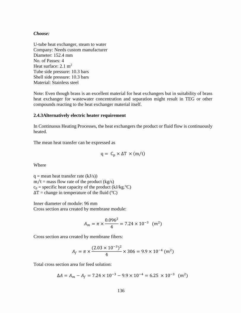
136
Choose:
U-tube heat exchanger, steam to water
Company: Needs custom manufacturer
Diameter: 152.4 mm
No. of Passes: 4
Heat surface: 2.1 m2
Tube side pressure: 10.3 bars
Shell side pressure: 10.3 bars
Material: Stainless steel
Note: Even though brass is an excellent material for heat exchangers but in suitability of brass
heat exchanger for wastewater concentration and separation might result in TEG or other
compounds reacting to the heat exchanger material itself.
2.4.3Alternatively electric heater requirement
In Continuous Heating Processes, the heat exchangers the product or fluid flow is continuously
heated.
The mean heat transfer can be expressed as
q = Cp × ∆T × (m t⁄ )
Where
q = mean heat transfer rate (kJ/s))
m t ⁄ = mass flow rate of the product (kg/s)
cp = specific heat capacity of the product (kJ/kg.oC)
∆T = change in temperature of the fluid (oC)
Inner diameter of module: 96 mm
Cross section area created by membrane module:
𝐴𝑚 = 𝜋 ×0.0962
4= 7.24 × 10⁻³ (𝑚2)
Cross section area created by membrane fibers:
𝐴𝑓 = 𝜋 ×(2.03 × 10⁻³)2
4× 306 = 9.9 × 10⁻⁴ (𝑚2)
Total cross section area for feed solution:
∆𝐴 = 𝐴𝑚 − 𝐴𝑓 = 7.24 × 10⁻³ − 9.9 × 10−4 = 6.25 × 10⁻³ (𝑚2)
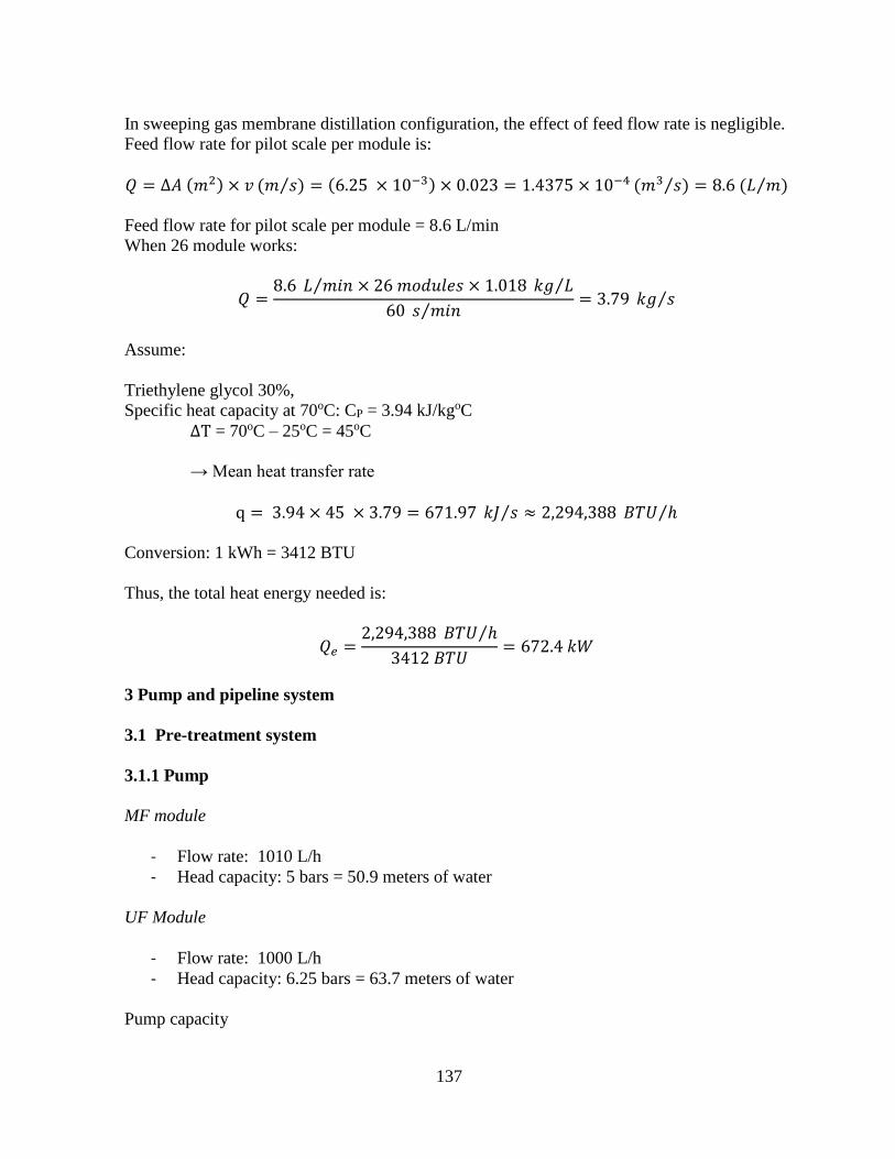
137
In sweeping gas membrane distillation configuration, the effect of feed flow rate is negligible.
Feed flow rate for pilot scale per module is:
𝑄 = ∆𝐴 (𝑚2) × 𝑣 (𝑚 𝑠)⁄ = (6.25 × 10−3) × 0.023 = 1.4375 × 10⁻⁴ (𝑚3 𝑠⁄ ) = 8.6 (𝐿 𝑚⁄ )
Feed flow rate for pilot scale per module = 8.6 L/min
When 26 module works:
𝑄 =8.6 𝐿 𝑚𝑖𝑛⁄ × 26 𝑚𝑜𝑑𝑢𝑙𝑒𝑠 × 1.018 𝑘𝑔 𝐿⁄
60 𝑠 𝑚𝑖𝑛⁄= 3.79 𝑘𝑔 𝑠⁄
Assume:
Triethylene glycol 30%,
Specific heat capacity at 70oC: CP = 3.94 kJ/kgoC
∆T = 70oC – 25oC = 45oC
→ Mean heat transfer rate
q = 3.94 × 45 × 3.79 = 671.97 𝑘𝐽 𝑠⁄ ≈ 2,294,388 𝐵𝑇𝑈 ℎ⁄
Conversion: 1 kWh = 3412 BTU
Thus, the total heat energy needed is:
𝑄𝑒 =2,294,388 𝐵𝑇𝑈 ℎ⁄
3412 𝐵𝑇𝑈= 672.4 𝑘𝑊
3 Pump and pipeline system
3.1 Pre-treatment system
3.1.1 Pump
MF module
- Flow rate: 1010 L/h
- Head capacity: 5 bars = 50.9 meters of water
UF Module
- Flow rate: 1000 L/h
- Head capacity: 6.25 bars = 63.7 meters of water
Pump capacity

138
P = Q. ρ. g. H
3.6 × 10⁶. η=
1.01 m3 h × 1125 kg m3 × 9.81 m s2⁄ × 63.7 m⁄⁄
3.6 × 106 × 0.65
= 0.3 KW = 0.4 Hp
Where:
ρ: Specific density of TEG wastewater, choose ρ = 1125 kg/m3 (for pure TEG)
η: pumping coefficient, choose η=0.65
Table B.6 Characteristics of Pre-treatment Pump
Descriptions Characteristics
Company Name ProMinent, Germany
Model DFCa 040
Pump capacity 1583 L/h
Pressure Max. 8 bars
Connector size 1.5 inch
Weight 89 kg
Feed rates 0.43- 15.83 L/rev
Self-priming up to 8m
Hose diameter (inside) 35 mm
Number of Pump 2
3.1.2 Pipeline system
Flow rate: 1000-1010 L/h
Wastewater velocity: v = 1-5 m/s (Metcalf and Eddy, 2005)
Assume v= 2 m/s
D = √4. Q
π. v= √
4 × 10¹⁰ L h⁄
π × 2 m s⁄= 13.36 mm
Choose:
Company name: MISUMI Thailand
Material: Vinyl Chloride
Model: PVCH No. 13
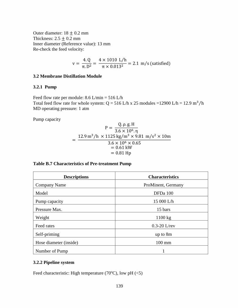
139
Outer diameter: 18 ± 0.2 mm
Thickness: 2.5 ± 0.2 mm
Inner diameter (Reference value): 13 mm
Re-check the feed velocity:
v = 4. Q
π. D2=
4 × 10¹⁰ L h⁄
π × 0.0132= 2.1 m s⁄ (satisfied)
3.2 Membrane Distillation Module
3.2.1 Pump
Feed flow rate per module: 8.6 L/min = 516 L/h
Total feed flow rate for whole system: Q = 516 L/h x 25 modules =12900 L/h = 12.9 m3 h⁄
MD operating pressure: 1 atm
Pump capacity
P = Q. ρ. g. H
3.6 × 10⁶. η
= 12.9 m3 h × 1125 kg m3 × 9.81 m s2⁄ × 10m⁄⁄
3.6 × 106 × 0.65
= 0.61 kW
= 0.81 Hp
Table B.7 Characteristics of Pre-treatment Pump
Descriptions Characteristics
Company Name ProMinent, Germany
Model DFDa 100
Pump capacity 15 000 L/h
Pressure Max. 15 bars
Weight 1100 kg
Feed rates 0.3-20 L/rev
Self-priming up to 8m
Hose diameter (inside) 100 mm
Number of Pump 1
3.2.2 Pipeline system
Feed characteristic: High temperature (70oC), low pH (<5)
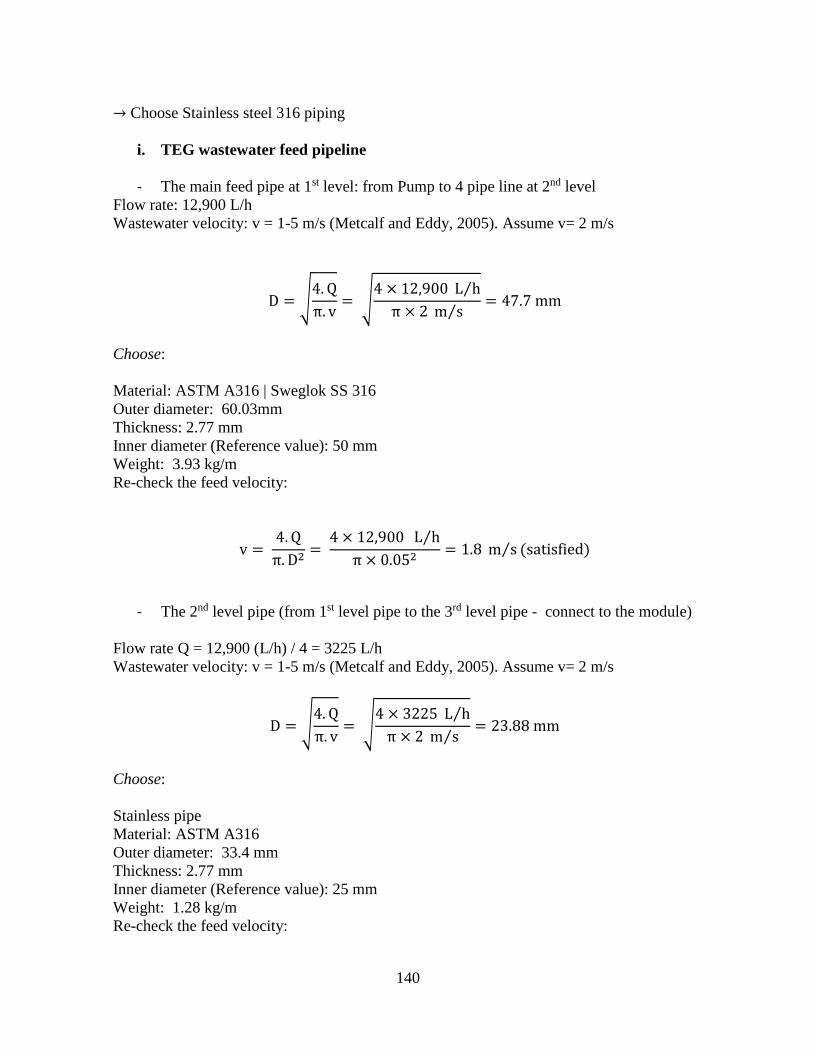
140
→ Choose Stainless steel 316 piping
i. TEG wastewater feed pipeline
- The main feed pipe at 1st level: from Pump to 4 pipe line at 2nd level
Flow rate: 12,900 L/h
Wastewater velocity: v = 1-5 m/s (Metcalf and Eddy, 2005). Assume v= 2 m/s
D = √4. Q
π. v= √
4 × 12,900 L h⁄
π × 2 m s⁄= 47.7 mm
Choose:
Material: ASTM A316 | Sweglok SS 316
Outer diameter: 60.03mm
Thickness: 2.77 mm
Inner diameter (Reference value): 50 mm
Weight: 3.93 kg/m
Re-check the feed velocity:
v = 4. Q
π. D2=
4 × 12,900 L h⁄
π × 0.052= 1.8 m s⁄ (satisfied)
- The 2nd level pipe (from 1st level pipe to the 3rd level pipe - connect to the module)
Flow rate Q = 12,900 (L/h) / 4 = 3225 L/h
Wastewater velocity: v = 1-5 m/s (Metcalf and Eddy, 2005). Assume v= 2 m/s
D = √4. Q
π. v= √
4 × 3225 L h⁄
π × 2 m s⁄= 23.88 mm
Choose:
Stainless pipe
Material: ASTM A316
Outer diameter: 33.4 mm
Thickness: 2.77 mm
Inner diameter (Reference value): 25 mm
Weight: 1.28 kg/m
Re-check the feed velocity:

141
v = 4. Q
π. D2=
4 × 3225 L h⁄
π × 0.0252= 1.8 m s⁄ (satisfied)
- The 3rd level pipe (from the 2nd level pipe to each membrane module)
Flow rate Q = 8.6 L/min
Wastewater velocity: v = 1-5 m/s (Metcalf and Eddy, 2005). Assume v= 2 m/s
D = √4. Q
π. v= √
4 × 8.6 L min⁄
π × 2 m s⁄= 9.55 mm
Choose:
Stainless pipe
Material: ASTM A316
Outer diameter: 17.15 mm
Thickness: 1.65 mm
Iner diameter (Reference value): 10 mm
Weight: 0.85 kg/m
Re-check the feed velocity:
v = 4. Q
π. D2=
4 × 8.6 L min⁄
π × 0.012= 1.8 m s⁄ (satisfied)
ii. Sweeping gas pipeline
Sweeping gas characteristic: Natural atmospheric gas
- The main gas pipe at 1st level: from Pump to 4 pipe line at 2nd level
Flow rate: 2028.8 L/min
Gas velocity: v = 10-20 m/s (Metcalf and Eddy, 2005). Assume v= 15 m/s
D = √4. Q
π. v= √
4 × 2028.8 L min⁄
π × 15 m s⁄= 53.57 mm
Choose:
Stainless pipe

142
Material: ASTM A316
Outer diameter: 60.03mm
Thickness: 2.77 mm
Inner diameter (Reference value): 50 mm
Weight: 3.93 kg/m
Re-check the feed velocity:
v = 4. Q
π. D2=
4 × 2028.8 L min⁄
π × 0.052= 17.22 m s⁄ (satisfied)
- The 2nd level pipe (from 1st level pipe to the 3rd level pipe - connect to the module)
Flow rate Q = 2028.8 (L/min) / 2 = 1014.4 L/min
Gas velocity: v = 10-20 m/s (Metcalf and Eddy, 2005). Assume v= 15 m/s
D = √4. Q
π. v= √
4 × 1014.4 L min⁄
π × 15 m s⁄= 37.8 mm
Choose:
Stainless pipe
Material: ASTM A316
Outer diameter: 48.26 mm
Thickness: 2.77 mm
Inner diameter (Reference value): 40 mm
Weight: 3.11 kg/m
Re-check the feed velocity:
v = 4. Q
π. D2=
4 × 1014.4 L min⁄
π × 0.042= 13.45 m s⁄ (satisfied)
- The 3rd level pipe (from the 2nd level pipe to each membrane module)
Flow rate Qgas = 0.255 L/ min × 306 fibers = 78.03 L/min
Gas velocity: v = 10-20 m/s (Metcalf and Eddy, 2005). Assume v= 15 m/s
D = √4. Q
π. v= √
4 × 78.03 L/min
π × 15 m s⁄= 10.05 mm
Choose:
Stainless pipe
143
Material: ASTM A316
Outer diameter: 17.15 mm
Thickness: 1.65 mm
Inner diameter (Reference value): 10 mm
Weight: 0.85 kg/m
Re-check the feed velocity:
v = 4. Q
π. D2=
4 × 78.03 L/min
π × 0.012= 16.6 m s⁄ (satisfied)
4 Clean in Place (CIP)
4.1 Pre-treatment system
After a certain operating time, the MF/UF membrane system needs to be cleaned. This is on
demand of membrane filtration.
Top Backwash Step
When the TMP exceeds 1 bar above starting TMP (at same temperature), the membrane system
should be stop to conduct the cleaning step. The clean water is provided from the inside space
of hollow fiber to the outside. The wastewater is drained out from the top of module housing.
This step is carried out to remove particulates at the highest concentration.
Duration: 15 minutes
Cleaning solution source: Tap water
Backwash pressure: 8 bars
Amount of tap water required
a) MF module
- Back wash flux: 50 L/m2.h
- Volume of water required:
V𝑀𝐹 = 50 (L m2. h)⁄ × 21 m2 × 0.25 h
= 262.5 L
b) UF module
- Back wash flux: 40 L/m2.h
- Volume of water required:
V𝑈𝐹 = 40 (L m2. h)⁄ × 33 m2 × 0.25 h = 330 L
Bottom Backwash Step

144
Similar with top backwash, the clean water flow pass membrane pores by inside-out mode. In
this step, backwash water is drained off from the bottom of module. The purpose is to remove
heavier materials which cannot remove by top backwash.
Forward flush
Depending on the degree of fouling, backwash step can be repeated a numerous times (normally
from 3 to 8 times). After that, the pre-treatment system was returned back to the normal
operating mode.
Chemical enhanced cleaning
Duration: 120 minutes (recycle and soak)
Cleaning Solutions: 0.2 % HCl, and 0.1% NaOH
Cleaning flux per Module: 1.0-1.5 m3/h
Temperature range: 10 to 40oC
Frequency: In the range from 1 to 3 months.
4.2 Membrane Distillation System Cleaning
Pure water cleaning
In MD technology, fouling phenomena is not a serious operating problem. Deposited particulars
can be removed by the turbulent velocity of water flow. Thus, tap water is used to clean the
fiber surface and shell surface.
Duration: 30 minutes
Frequency: 1 time per week
Cleaning solution: Pure water
Volume of pure water: 300 L
Cleaning procedure: The cleaning mode is by-pass. Pure water will not be heat up and sweeping
gas will not be provided. The cleaning wastewater was recirculated back to the feed tank. After
that, it was drained out to the sewer system.
This step can be repeated a numerous times to achieve a good cleaned module.
Chemical cleaning
When operating with wastewater (either synthetic or real wastewater), boundary layer was
formed on the membrane surface. Consequently, fouling resistance will contribute to total
resistance. It will result in decreasing of permeate flux along with timeline of operational
process.
Chemical agents which will use to clean the hydrophobic membrane are a mixture of oxalic and
citric acid. This cleaning solution has been proven as an efficient solution to clean the
hydrophobic membrane distillation. Time of cleaning period and chemical concentration are
shown in Table B.8.
145
Table B.8 Chemical Concentration for Membrane Cleaning
Step Cleaning
procedure
Concentration
(mg/L) pH
Cleaning
Time (h) Purpose
1 Water (1) - 6.15 0.5 Recoverable fouling
2 Oxalic/Citric
0.1wt. % Oxalic acid
and
0.8wt. % Citric acid
2.2 6 Reversible fouling
3 Water (2) - 6.15 0.5 Washing the remain
chemical
4 Sunlight 24 Dry-out
The procedure is similar with pure water cleaning step. However, chemicals are weighted and
put directly into the feed tank. The chemical solution was mixed evenly by the feed pump.
Frequency: 1 time per month
Total chemical liquid volume: 300 L
Amount of acid per time of cleaning: 0.3 kg Oxalic acid (0.1 wt%) and 2.4 kg Citric acid (0.8
wt%)
Clean water storage tank
Total minimum volume required for both pre-treatment system and MD system:
V = VMF + VUF + VMD = 262.5 + 330 + 300 = 892.5 L Choose
Model: CEN2K0A-M107
Manufacturer: PAKCO International Co., Ltd.
Material: Polyethylene (PE)
Dimension: B = 395mm, C = 1300 mm, H = 1900 mm, h = 1650 mm, K = 395 mm, O = 90
mm. Thickness = 10 mm.
Capacity: 2 m3
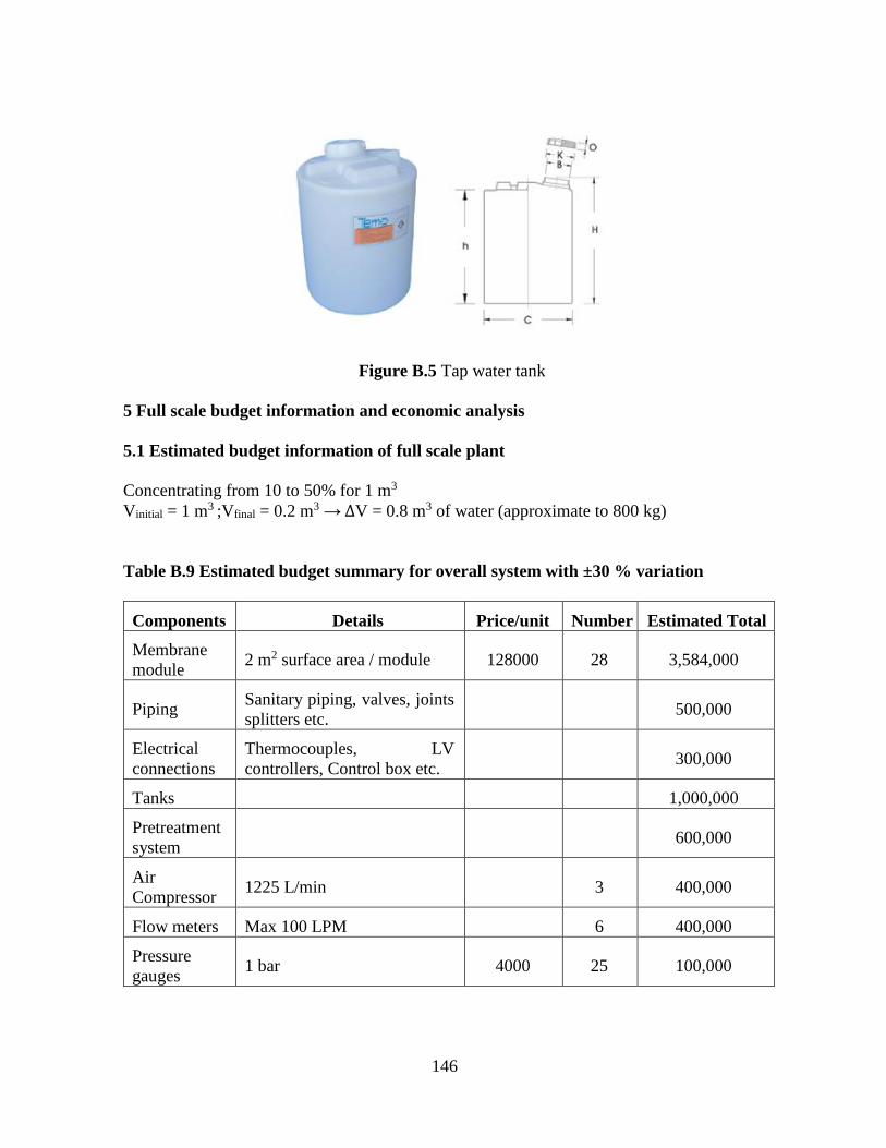
146
Figure B.5 Tap water tank
5 Full scale budget information and economic analysis
5.1 Estimated budget information of full scale plant
Concentrating from 10 to 50% for 1 m3
Vinitial = 1 m3 ;Vfinal = 0.2 m3 → ∆V = 0.8 m3 of water (approximate to 800 kg)
Table B.9 Estimated budget summary for overall system with ±30 % variation
Components Details Price/unit Number Estimated Total
Membrane
module 2 m2 surface area / module 128000 28 3,584,000
Piping Sanitary piping, valves, joints
splitters etc. 500,000
Electrical
connections
Thermocouples, LV
controllers, Control box etc. 300,000
Tanks 1,000,000
Pretreatment
system 600,000
Air
Compressor 1225 L/min 3 400,000
Flow meters Max 100 LPM 6 400,000
Pressure
gauges 1 bar 4000 25 100,000
147
Pressure
gauges 5 Bar 3000 3 9,000
Pumps
100 LPM (Circulation pump
for MF) 1 60,000
100 LPM (Circulation pump
for UF, 5 Bar) 1 60,000
500 LPM (Circulation pump
for MD) 1 100,000
Heat exchanger Maintain temp 70 Deg C for
0.5 m3 water 1 400,000
Total 6,493,000
5.2 Energy Analysis
In technology innovation, energy consumption of MD process is an important factor for this
energy intensive technology. The components consuming energy in MD process are: thermal
energy to heat the feed liquid, energy required for circulation pump and compressor. The heat
energy requirement is more than 90% of the total energy consumption of MD process (M.
Khayet and Matsuura, 2011)
The balance of heat energy is shown in Equation below
𝑄𝑚 = 𝑄𝑐 + 𝑄𝑣
Where Qm, Qv, Qc are total heat transfer in MD process, heat transfer by mass transfer and heat
transfer by conduction of membrane respectively
𝑄𝑣 = 𝐽𝑤 × ∆𝐻𝑣,𝑤 = 1.95 𝑘𝑔 𝑚2. ℎ⁄ × 2270 𝑘𝐽 𝑘𝑔⁄ = 4426.5 𝑘𝐽 𝑚2. ℎ⁄
𝑄𝑐 =𝑘𝑚
𝛿× (𝑇𝑚𝑓 − 𝑇𝑚𝑝) =
0.14 𝑊 𝑚. 𝐾⁄
0.00048 𝑚× (67.7 − 66.6) = 320.8
Thermal efficiency, η
η =Qv
Qv + Qc× 100 =
4426.5
4426.5 + 320.8× 100 = 93.2 %
𝑄𝑐 is considered as heat loss. The thermal efficiency in SGMD is very high (93.2%) while that
value for DCMD is between 50-80% (Khayet and Matsuura, 2011). Thus, it can be concluded
that the heat loss is not significant in MD process.

148
Figure B.6 Energy consumption/Qp of continuously-fed real wastewater investigation
The average energy required to concentrate TEG in real wastewater from 10 to 60 % is 0.624
kW/kg (624 kW/m3). Energy consumption had been evaluated for DCMD and VMD at lab scale
(Criscuoli et al., 2008). The authors conducted a study on plate-and- frame membrane module
(membrane area of 40 cm2). The lowest ratio of energy consumption/Qp obtained were 3546.3
kW/m3 and 1108.4 kW/m3 in DCMD and VMD respectively. The performance of VMD was
proven to be better than DCMD (based on permeate flux, energy consumption and thermal
efficiency). As yet, almost studies were done theoretical modeling. Thus, it is very important to
conduct study on realistic energy consumption.
5.3 SGMD Costs Evaluations
The annual operating cost is the yearly purchase to own and operate MD system. This amount
include amortization, O&M costs and membrane replacement cost.
5.3.1 Amortization or fixed charges
This annual interest payment is normally charged to cover the initial capital cost when the fund
is borrowed.
Amortization factor (a) is calculated as
a =i × (1 + i)n
(1 + i)n − 1
5
15
25
35
45
55
65
0.0
0.2
0.4
0.6
0.8
1.0
0 5 10 15 20 25 30 35 40 45
TE
G c
on
cen
trat
ion
(%)
En
ergy r
atio
(kW
/kg)
Time (h)
Energy ratio TEG concentration
149
Where i, n are the annual interest rate (%) and the year of life time of MD system.
Assume i = 0.05 (5%) and n = 20 years (Banat and Jwaied, 2008)
a =0.05 × (1 + 0.05)20
(1 + 0.05)20 − 1= 0.080243 (year−1)
Therefore, the annual fixed charges is:
Afixed = a × capital cost = 0.080243 × 6,493,000 baht = 521,017.8 baht year⁄
5.3.2 O &M costs
The annual maintenance and operation costs are estimated to account for 20% of the plant
annual payment (Khayet and Matsuura, 2011)
𝐴𝑂&𝑀 = 0.2 × Afixed = 0.2 × 521,017.8 = 104,203.6 baht year⁄
5.3.3 Membrane Replacement costs
This is the cost required for membrane replacement. It is a function of production process.
Membrane replacement cost is calculated as 20% of the membrane module cost.
𝐴𝑀𝑅 = 0.2 × MC = 0.2 × 3,584,000 = 716,800 baht year⁄
5.3.4 Plant Availability (f)
Plant availability means the total working time of the plant per year. It can be assumed to be
90% per year (Khayet and Matsuura, 2011).
5.3.5 Electricity cost (𝑨𝒆𝒍𝒆𝒄𝒕𝒓𝒊𝒄)
A𝑒𝑙𝑒𝑐𝑡𝑟𝑖𝑐 = 𝑐 × 𝜔 × f. M. 365
Where 𝑐, 𝜔, f, M are electric cost (3 baht/kWh), specific energy consumption (kWh/m3), plant
availability (90%) and plant capacity (1 m3/d) respectively.
Specific energy consumption (0.624 kWh/kg), concentrate TEG from 10 to 50%. Thus the total
volume reduce from 1000 L (1 m3) to 200 L
𝜔 = 0.624 × (1000 − 200) = 499.2 kWh/m3
Thus,

150
A𝑒𝑙𝑒𝑐𝑡𝑟𝑖𝑐 = 𝑐 × 𝜔 × f. M. 365
= 3 baht kWh⁄ × 499.2 kWh m3⁄ × 0.9 × 365 days year⁄ × 1 m3 day⁄
= 491,961.6 baht year⁄
5.3.6 Labour cost (Alabour)
A𝑙𝑎𝑏𝑜𝑢𝑟 = 𝑔. f. M. 365
Where g (500 baht/m3) is specific labour cost
A𝑙𝑎𝑏𝑜𝑢𝑟 = 500 baht m3⁄ × 0.9 × 365 days year⁄ × 1 m3 day⁄ = 164,250 baht year⁄
Therefore, the total annual cost (Atotal)
𝐴𝑡𝑜𝑡𝑎𝑙 = 𝐴𝑓𝑖𝑥𝑒𝑑 + 𝐴𝑂&𝑀 + 𝐴𝑀𝑅 + A𝑒𝑙𝑒𝑐𝑡𝑟𝑖𝑐 + A𝑙𝑎𝑏𝑜𝑢𝑟
= 521,017.8 + 104,203.6 + 716,800 + 491,961.6 + 164,250 = 1,998,232.9 baht year⁄
Treatment cost based on the total annual cost
TC =Atotal
f. M. 365=
1,998,232.9 baht year⁄
0.9 × 365 days year⁄ × 1 m3 day⁄ = 6,082.9 baht m3⁄
Treatment cost based on Electricity cost, Labour cost, O &M costs
TC =156,305.3 + 491,961.6 + 104,203.6 baht year⁄
0.9 × 365 days year⁄ × 1 m3 day⁄ = 2290.6 baht m3⁄
Chemical cleaning of MD system
Frequency: 1 time per month
Total chemical liquid volume: 300 L
Amount of acid per time of cleaning: 0.3 kg Oxalic acid (0.1 wt%) and 2.4 kg Citric
acid (0.8 wt%)
Total amount of chemicals using per year:
W𝑎𝑐𝑖𝑑𝑠 = W𝐶𝑖𝑡𝑟𝑖𝑐 + W𝑂𝑥𝑎𝑙𝑖𝑐 = (2.4 𝑘𝑔 + 0.3 𝑘𝑔) × 12 𝑚𝑜𝑛𝑡ℎ𝑠 = 32.4 𝑘𝑔
Chemicals cost per year
𝐴𝑐ℎ𝑒𝑚𝑖𝑐𝑎𝑙𝑠 = 32.4 𝑘𝑔 × 1,000 𝑏𝑎ℎ𝑡 𝑝𝑒𝑟 𝑘𝑔 = 32,400 𝑏𝑎ℎ𝑡
This chemical cost was included in annual O&M cost
151
Appendix C
Operational Manual of Pilot scale Sweeping Gas Membrane Distillation System

152
1. General information
1.1 Semi-pilot scale of pretreatment unit
The pre-treatment unit is a combined membrane system, hollow fiber ultrafiltration
membrane (UF) followed by cartridge microfiltration membrane (MF). This unit played
as a physical filtration barrier, to remove suspended solids (by MF), oil and grease (by UF).
The imagine of pre-treatment unit is expressed in Figure C.1. The air-to-water ratio was set
at 24. The purpose of adding air diffuser is to remove BTEX and transfer iron ion to ferric
hydroxide (Fe(OH)3)
Figure C.1 Schematic diagram of the semi-pilot scale pre-treatment unit
7. Raw WW Tank
8. MF Module
9. Intermediate Tank
10. UF Module
11. Pre-treated WW
12. Control box
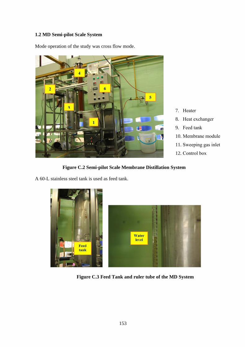
153
1.2 MD Semi-pilot Scale System
Mode operation of the study was cross flow mode.
Figure C.2 Semi-pilot Scale Membrane Distillation System
A 60-L stainless steel tank is used as feed tank.
Figure C.3 Feed Tank and ruler tube of the MD System
7. Heater
8. Heat exchanger
9. Feed tank
10. Membrane module
11. Sweeping gas inlet
12. Control box

154
2. System Operation Overview
2.1 Pre-treatment System
Figure C.4 Pre-treatment system
2.1.1 Oparational Steps
1. Check all the tubes and connectors first.
2. Check the MF membrane housing is tight enough.
3. Fill the Waste water to Tank 1. (200 L)
4. Start air stripping- air is applied to the water in the ratio air-to-water of 24.
It need around 5 hours air stripping for 150 L with 13.6 L/m air flow. This depends
on Initial BTEX concentration.
5. Switch on the system. (Control box switch)
6. Keep fully open the baypass valves initially. (Both MF and UF)
7. Switch on the “Run switch”.
8. Then slowly close the bypass valve and see the pressure gauge 1. Pressure should
be about 1 bar. Adjust pressure with bypass valve.
9. Press the air release valve on MF membran housing and release the air initially.
When water come out from the releasin button, un press it.
10. When Pump 2 works, slowly adgust the pressure on UF membranes by UF bypass
valve. Pressure should be below 2-4 bar.
11. Check the permeate line whether fulx is commig or not. Permeate will come after
adjusting the pressure on UF membrane.
12. System will automatically run after this.
2.1.2 Cleaning pre-treatment system membranes
1. Remove the housing of the cartridge MF membrane.
Raw wastewater tank
D
Intermediate tank Pre-treated tank
UF Module MF Module
P
Air
P P
Level Sensor D Air Diffuser P Pressure Gauge
Pump Valve
Tank
1 Tank
2
Tank
3

155
2. Safely remove the ceramic MF membrane.
3. Simply add water and remove solids with a sponge.
4. Sponge it only one direction.
2.2 MD Semi-Pilot Scale System
MF Filter Cartridge after
filtration
MF Filter Cartridge after
cleaning

156
T
L
F/T
T
T
T
Permeate
tank
Heat
exchanger
Heat
exchanger
Heat
exchanger
Chiller
Air compressor
Chiller
Heater
Feed tank
Hollow fiber
module
F/T TPump Pressure gauge ValveThermocoupleAir fi lter/water traper L Level sensor
Permeate
measuring tube
Flow meter
1 2
3
4
Figure C.5 Schematic diagram of the semi-pilot scale MD system
2.2.1 Starting Up
1. Fill the pre-treated wastewater to feed tank.
2. Check the water bath water level initially and maintain the level with DI
water.
3. Switch on the heater and adjust the temperature. Then Switch on the
circulation pump of the heater.
4. Valve 1, 2 and 3 are to be closed and valve 4 is to be opened.
5. Then, feed pump is to be turned on and circulates the solution directly to
heat exchanger
2.2.2 Distilling
1. After reach desired temperature, valve 1 and 4 are need to close and valve
2 and 3 are to be opened.
2. Circulate feed solution through the membrane.
3. Then, ambient air is to be pumped into the membrane.
4. At this stage, inlet pressure of air has to be carefully adjust with pressure
regulator and matched with inlet of feed solution.
2.2.3 Permeate Flux Measurement
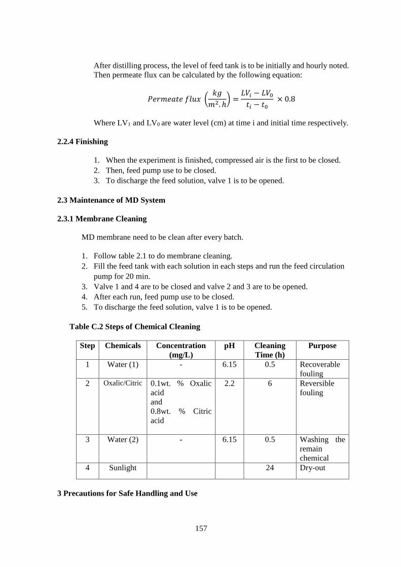
157
After distilling process, the level of feed tank is to be initially and hourly noted.
Then permeate flux can be calculated by the following equation:
𝑃𝑒𝑟𝑚𝑒𝑎𝑡𝑒 𝑓𝑙𝑢𝑥 (𝑘𝑔
𝑚2. ℎ) =
𝐿𝑉𝑖 − 𝐿𝑉0
𝑡𝑖 − 𝑡0 × 0.8
Where LV1 and LV0 are water level (cm) at time i and initial time respectively.
2.2.4 Finishing
1. When the experiment is finished, compressed air is the first to be closed.
2. Then, feed pump use to be closed.
3. To discharge the feed solution, valve 1 is to be opened.
2.3 Maintenance of MD System
2.3.1 Membrane Cleaning
MD membrane need to be clean after every batch.
1. Follow table 2.1 to do membrane cleaning.
2. Fill the feed tank with each solution in each steps and run the feed circulation
pump for 20 min.
3. Valve 1 and 4 are to be closed and valve 2 and 3 are to be opened.
4. After each run, feed pump use to be closed.
5. To discharge the feed solution, valve 1 is to be opened.
Table C.2 Steps of Chemical Cleaning
Step Chemicals Concentration
(mg/L)
pH Cleaning
Time (h)
Purpose
1 Water (1) - 6.15 0.5 Recoverable
fouling
2 Oxalic/Citric 0.1wt. % Oxalic
acid
and
0.8wt. % Citric
acid
2.2 6 Reversible
fouling
3 Water (2) - 6.15 0.5 Washing the
remain
chemical
4 Sunlight 24 Dry-out
3 Precautions for Safe Handling and Use
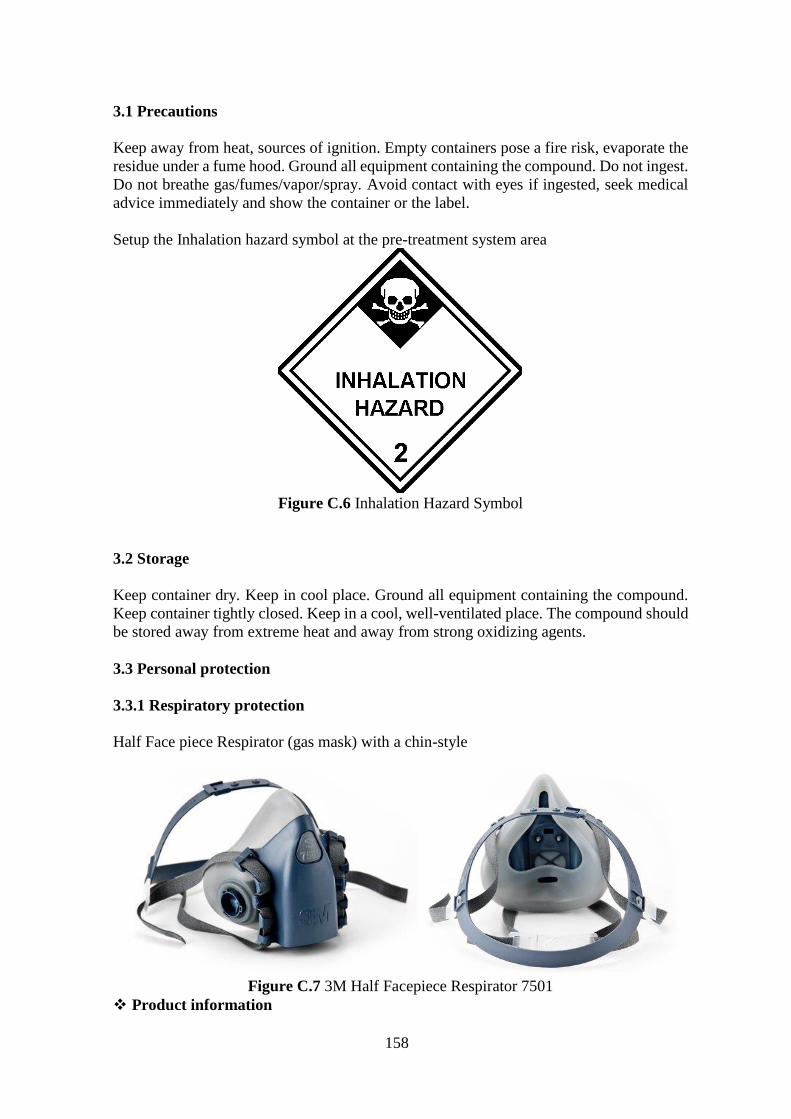
158
3.1 Precautions
Keep away from heat, sources of ignition. Empty containers pose a fire risk, evaporate the
residue under a fume hood. Ground all equipment containing the compound. Do not ingest.
Do not breathe gas/fumes/vapor/spray. Avoid contact with eyes if ingested, seek medical
advice immediately and show the container or the label.
Setup the Inhalation hazard symbol at the pre-treatment system area
Figure C.6 Inhalation Hazard Symbol
3.2 Storage
Keep container dry. Keep in cool place. Ground all equipment containing the compound.
Keep container tightly closed. Keep in a cool, well-ventilated place. The compound should
be stored away from extreme heat and away from strong oxidizing agents.
3.3 Personal protection
3.3.1 Respiratory protection
Half Face piece Respirator (gas mask) with a chin-style
Figure C.7 3M Half Facepiece Respirator 7501
Product information

159
Manufacturer: 3M Occupational Health and Environmental Safety Division (OH &
ESD), USA
Material: Silicone
Size: Small
Filter cartridge: Model 6003-NIOSH, use to avoid certain organic vapors, chlorine,
hydrogen chloride, and sulfur dioxide or hydrogen sulfide or hydrogen fluoride
Figure C.8 3M Half Facepiece Respirator with Cartridge 6003
Using guideline (suggested by the manufacturer)
Donning
(1) Adjust head cradle size as needed to fit comfortably on head.
(2) Place the respirator over the mouth and nose, then pull the head harness over the
crown of the head.
(3) Grasp the bottom straps, place them at the back of the neck and hook them together.
Pull the ends of the straps to adjust the tightness.
(4) Do not over-tighten. Perform a positive and/or negative pressure user seal check
each time the respirator is donned.
User seal check
Always check the seal of the respirator on your face before entering a contaminated
area. Inhale gently.
(1) If you feel facepiece collapse slightly and pull closer to your face with no leaks
between the face and facepiece, a proper seal has been obtained.
(2) If faceseal air leakage is detected, reposition respirator on face and/or readjust
tension of straps to eliminate air leakage.
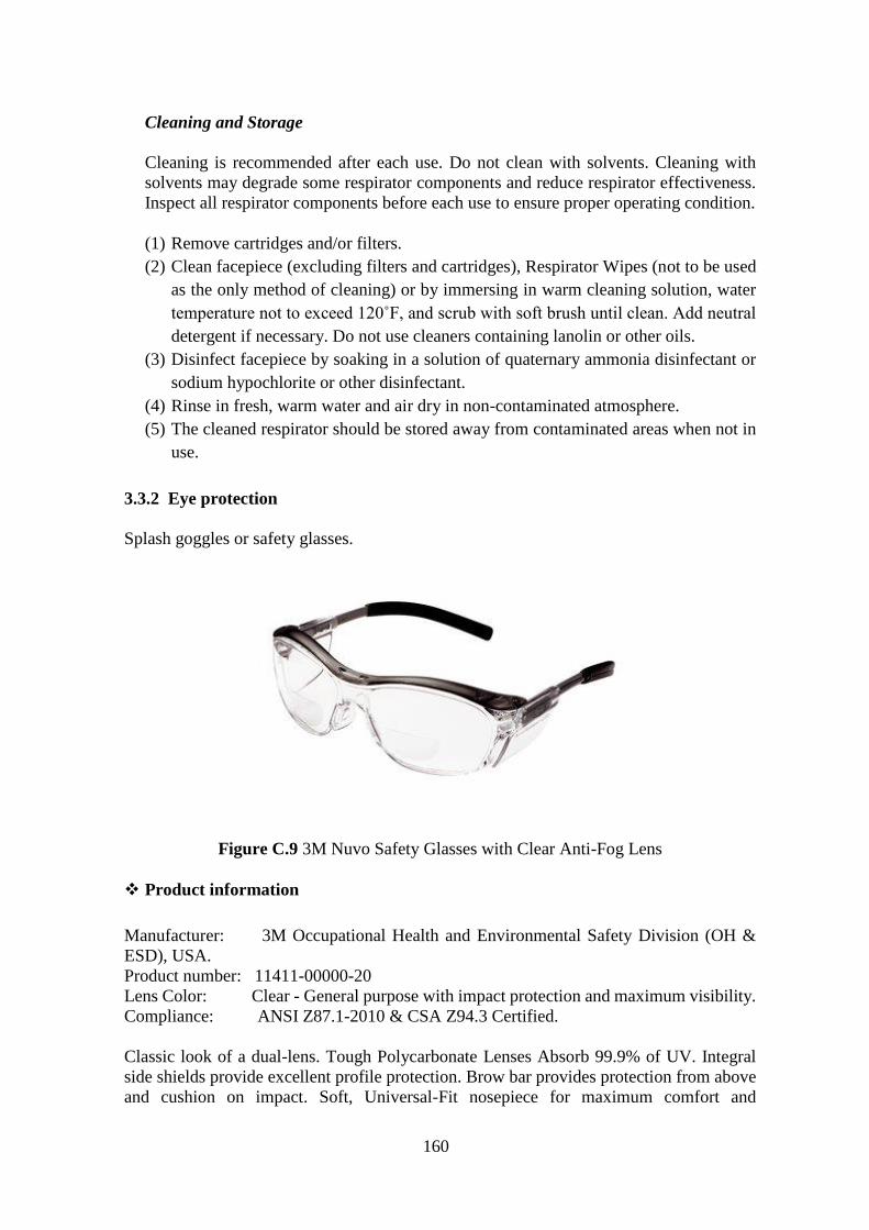
160
Cleaning and Storage
Cleaning is recommended after each use. Do not clean with solvents. Cleaning with
solvents may degrade some respirator components and reduce respirator effectiveness.
Inspect all respirator components before each use to ensure proper operating condition.
(1) Remove cartridges and/or filters.
(2) Clean facepiece (excluding filters and cartridges), Respirator Wipes (not to be used
as the only method of cleaning) or by immersing in warm cleaning solution, water
temperature not to exceed 120˚F, and scrub with soft brush until clean. Add neutral
detergent if necessary. Do not use cleaners containing lanolin or other oils.
(3) Disinfect facepiece by soaking in a solution of quaternary ammonia disinfectant or
sodium hypochlorite or other disinfectant.
(4) Rinse in fresh, warm water and air dry in non-contaminated atmosphere.
(5) The cleaned respirator should be stored away from contaminated areas when not in
use.
3.3.2 Eye protection
Splash goggles or safety glasses.
Figure C.9 3M Nuvo Safety Glasses with Clear Anti-Fog Lens
Product information
Manufacturer: 3M Occupational Health and Environmental Safety Division (OH &
ESD), USA.
Product number: 11411-00000-20
Lens Color: Clear - General purpose with impact protection and maximum visibility.
Compliance: ANSI Z87.1-2010 & CSA Z94.3 Certified.
Classic look of a dual-lens. Tough Polycarbonate Lenses Absorb 99.9% of UV. Integral
side shields provide excellent profile protection. Brow bar provides protection from above
and cushion on impact. Soft, Universal-Fit nosepiece for maximum comfort and
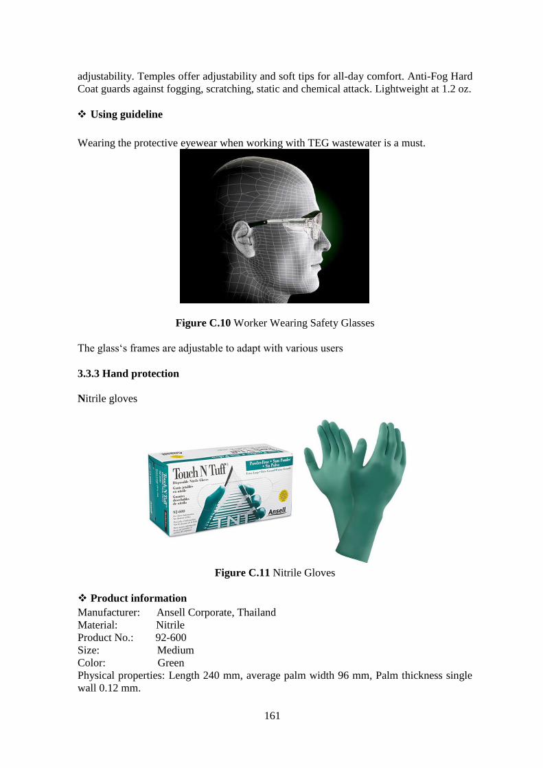
161
adjustability. Temples offer adjustability and soft tips for all-day comfort. Anti-Fog Hard
Coat guards against fogging, scratching, static and chemical attack. Lightweight at 1.2 oz.
Using guideline
Wearing the protective eyewear when working with TEG wastewater is a must.
Figure C.10 Worker Wearing Safety Glasses
The glass‘s frames are adjustable to adapt with various users
3.3.3 Hand protection
Nitrile gloves
Figure C.11 Nitrile Gloves
Product information
Manufacturer: Ansell Corporate, Thailand
Material: Nitrile
Product No.: 92-600
Size: Medium
Color: Green
Physical properties: Length 240 mm, average palm width 96 mm, Palm thickness single
wall 0.12 mm.

162
Features: Outstanding Chemical resistance, excellent puncture resistance, easy
donning and strong Grip.
Using guideline
Wearing the nitrile gloves when working with TEG wastewater is a must.
Figure C.12 Wearing Nitrile Glove
Use one time only. This is disposable product

163
Appendix D
Details of Calculations
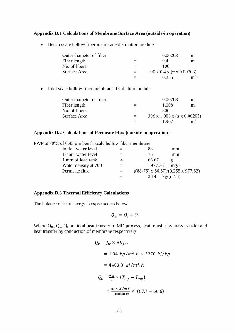
164
Appendix D.1 Calculations of Membrane Surface Area (outside-in operation)
Bench scale hollow fiber membrane distillation module
Outer diameter of fiber = 0.00203 m
Fiber length = 0.4 m
No. of fibers = 100
Surface Area = 100 x 0.4 x (π x 0.00203)
= 0.255 m2
Pilot scale hollow fiber membrane distillation module
Outer diameter of fiber = 0.00203 m
Fiber length = 1.008 m
No. of fibers = 306
Surface Area = 306 x 1.008 x (π x 0.00203)
= 1.967 m2
Appendix D.2 Calculations of Permeate Flux (outside-in operation)
PWF at 70oC of 0.45 µm bench scale hollow fiber membrane
Initial water level = 88 mm
1-hour water level = 76 mm
1 mm of feed tank ≅ 66.67 g
Water density at 70oC = 977.36 mg/L
Permeate flux = ((88-76) x 66.67)/(0.255 x 977.63)
= 3.14 kg/(m2.h)
Appendix D.3 Thermal Efficiency Calculations
The balance of heat energy is expressed as below
𝑄𝑚 = 𝑄𝑐 + 𝑄𝑣
Where Qm, Qv, Qc are total heat transfer in MD process, heat transfer by mass transfer and
heat transfer by conduction of membrane respectively
𝑄𝑣 = 𝐽𝑤 × ∆𝐻𝑣,𝑤
= 1.94 𝑘𝑔 𝑚2. ℎ⁄ × 2270 𝑘𝐽 𝑘𝑔⁄
= 4403.8 𝑘𝐽 𝑚2. ℎ⁄
𝑄𝑐 =𝑘𝑚
𝛿× (𝑇𝑚𝑓 − 𝑇𝑚𝑝)
=0.14 𝑊 𝑚.𝐾⁄
0.00048 𝑚× (67.7 − 66.6)

165
= 320.8 𝑘𝐽 𝑚2. ℎ⁄
Thermal efficiency, η
η =Qv
Qv+Qc× 100
=4403.8
4403.8 + 320.8× 100
= 93.2 %
𝑄𝑐 is considered as heat loss.
Appendix D.4 Flow Simulation and Heat Transfer Calculation
Pilot Scale Membrane Distillation Membrane Module
Velocity Distribution
Initially, the pilot scale hollow fiber membrane distillation was designed with the length of
1,105 mm and the diameter of flow channel was 47.6 mm. Whereas, the diameter of inlet
pipe was 23 mm. With the inlet flow rate of 60 L/min, the flow velocity in the inlet pipe
was 2.4 L/min, meanwhile the theoretical average value inside the module was 0.16 m/s.
As soon as the high fluid velocity exposed to the hollow fiber at the module’s entrance, it
would damage the fiber. Besides, the hollow fibers also acted as a barrier of fluid entrance.
The flow simulation was done to simulate the characteristic of liquid flow inside the
module (local velocity, local flow direction). The boundary condition was set at: inlet flow
of 1 L/s (60 L/min) and outlet flow at atmospheric pressure. The flow temperature was
70oC with the fluid density of 977.84 kg/m3.
The simulated results by using Solidworks software were shown in Table D.1 and Figure
D.1.
Table D.1 Computational Flow Simulation Results
Name Unit Value Delta
Minimum Velocity m/s -1.030 0.0105
Average Velocity m/s 0.164 5.1687 x 10⁻⁶
Maximum Velocity m/s 3.350 0.0036
Maximum Reynolds number 394,700.3 425.9
Average Reynolds number 19,371.7 0.609
Minimum Reynolds number -121,295.7 1235.6
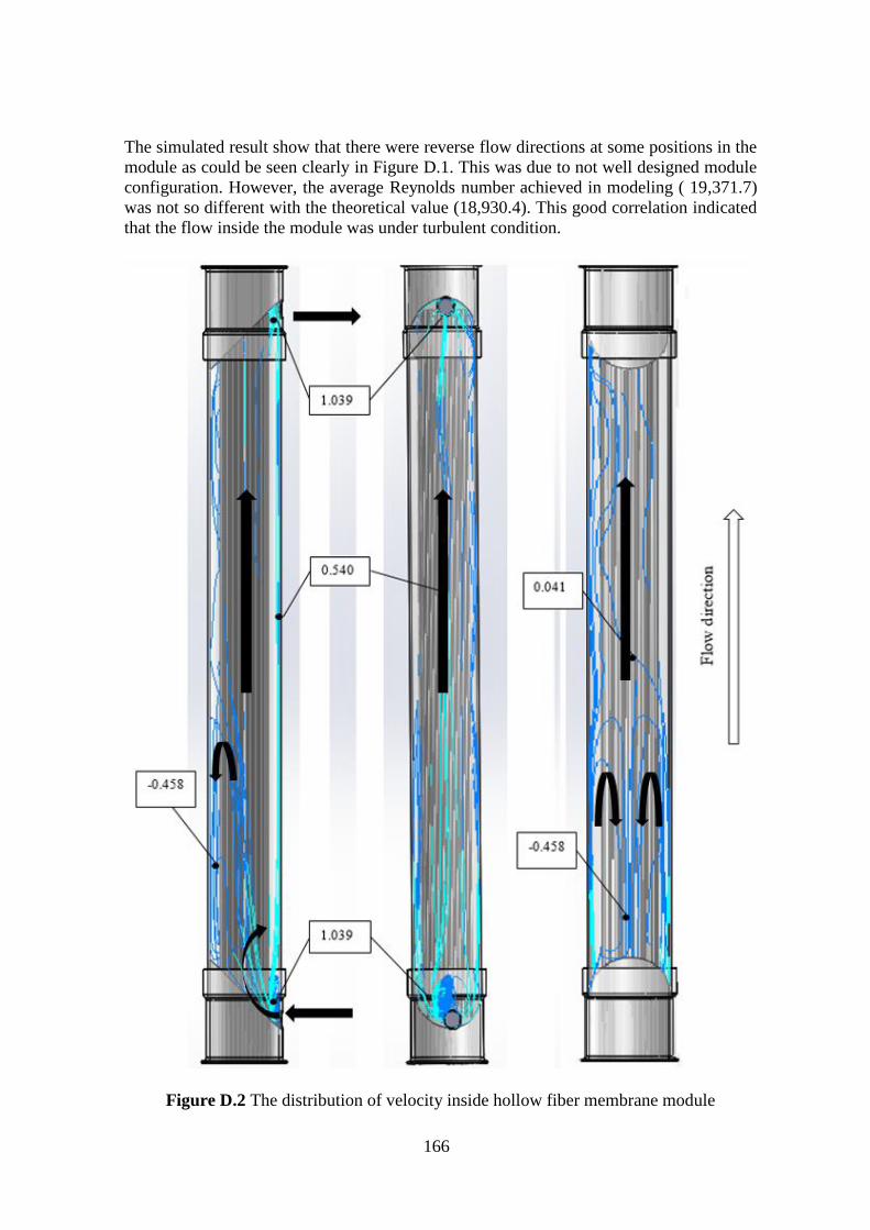
166
The simulated result show that there were reverse flow directions at some positions in the
module as could be seen clearly in Figure D.1. This was due to not well designed module
configuration. However, the average Reynolds number achieved in modeling ( 19,371.7)
was not so different with the theoretical value (18,930.4). This good correlation indicated
that the flow inside the module was under turbulent condition.
Figure D.2 The distribution of velocity inside hollow fiber membrane module
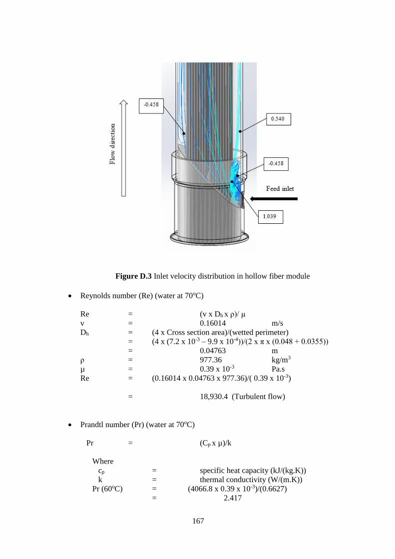
167
Figure D.3 Inlet velocity distribution in hollow fiber module
Reynolds number (Re) (water at 70oC)
Re = (v x Dh x ρ)/ µ
v = 0.16014 m/s
Dh = (4 x Cross section area)/(wetted perimeter)
= (4 x (7.2 x 10-3 – 9.9 x 10⁻⁴))/(2 x π x (0.048 + 0.0355))
= 0.04763 m
ρ = 977.36 kg/m3
µ = 0.39 x 10⁻³ Pa.s
Re = (0.16014 x 0.04763 x 977.36)/( 0.39 x 10⁻³)
= 18,930.4 (Turbulent flow)
Prandtl number (Pr) (water at 70oC)
Pr = (Cp x µ)/k
Where
cp = specific heat capacity (kJ/(kg.K))
k = thermal conductivity (W/(m.K))
Pr (60oC) = (4066.8 x 0.39 x 10-3)/(0.6627)
= 2.417
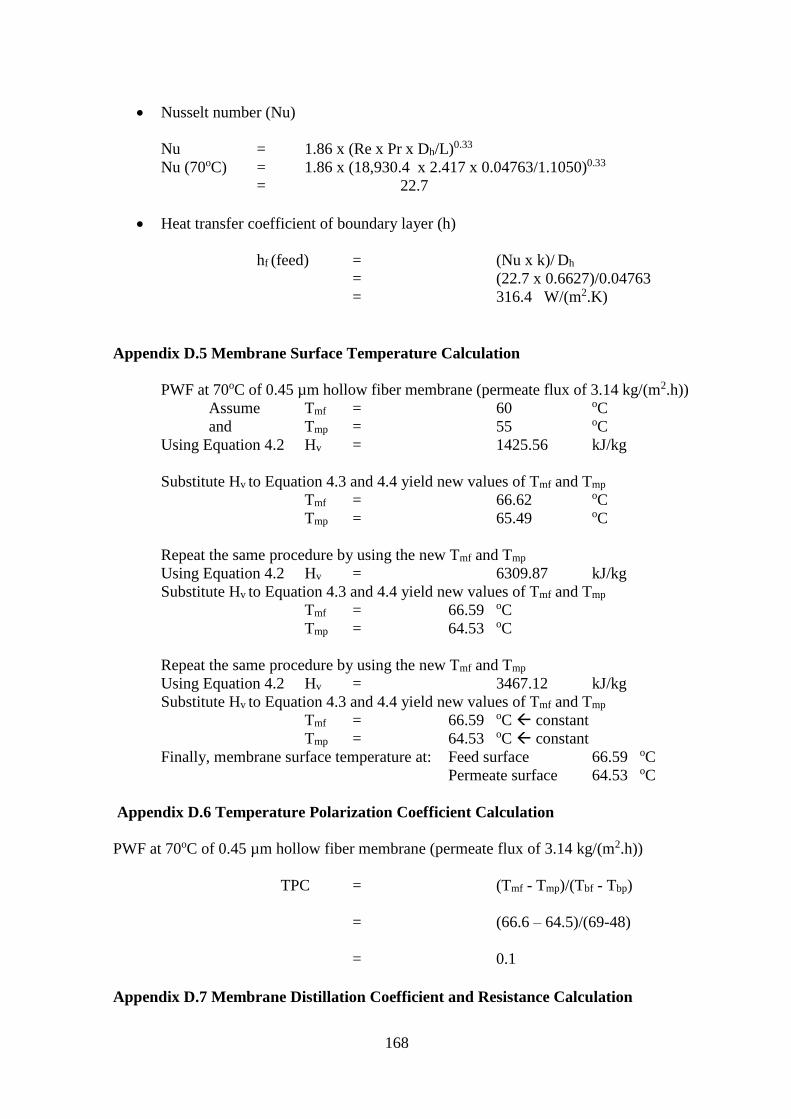
168
Nusselt number (Nu)
Nu = 1.86 x (Re x Pr x Dh/L)0.33
Nu (70oC) = 1.86 x (18,930.4 x 2.417 x 0.04763/1.1050)0.33
= 22.7
Heat transfer coefficient of boundary layer (h)
hf (feed) = (Nu x k)/ Dh
= (22.7 x 0.6627)/0.04763
= 316.4 W/(m2.K)
Appendix D.5 Membrane Surface Temperature Calculation
PWF at 70oC of 0.45 µm hollow fiber membrane (permeate flux of 3.14 kg/(m2.h))
Assume Tmf = 60 oC
and Tmp = 55 oC
Using Equation 4.2 Hv = 1425.56 kJ/kg
Substitute Hv to Equation 4.3 and 4.4 yield new values of Tmf and Tmp
Tmf = 66.62 oC
Tmp = 65.49 oC
Repeat the same procedure by using the new Tmf and Tmp
Using Equation 4.2 Hv = 6309.87 kJ/kg
Substitute Hv to Equation 4.3 and 4.4 yield new values of Tmf and Tmp
Tmf = 66.59 oC
Tmp = 64.53 oC
Repeat the same procedure by using the new Tmf and Tmp
Using Equation 4.2 Hv = 3467.12 kJ/kg
Substitute Hv to Equation 4.3 and 4.4 yield new values of Tmf and Tmp
Tmf = 66.59 oC constant
Tmp = 64.53 oC constant
Finally, membrane surface temperature at: Feed surface 66.59 oC
Permeate surface 64.53 oC
Appendix D.6 Temperature Polarization Coefficient Calculation
PWF at 70oC of 0.45 µm hollow fiber membrane (permeate flux of 3.14 kg/(m2.h))
TPC = (Tmf - Tmp)/(Tbf - Tbp)
= (66.6 – 64.5)/(69-48)
= 0.1
Appendix D.7 Membrane Distillation Coefficient and Resistance Calculation
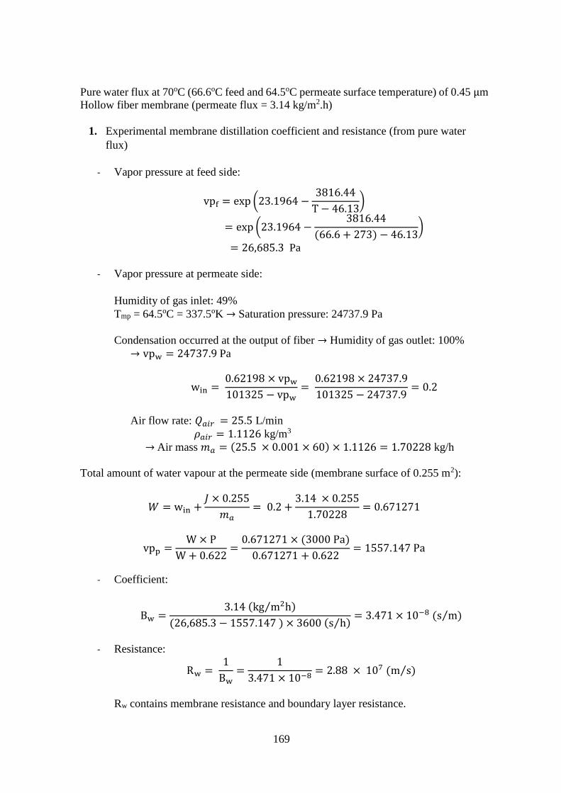
169
Pure water flux at 70oC (66.6oC feed and 64.5oC permeate surface temperature) of 0.45 µm
Hollow fiber membrane (permeate flux = 3.14 kg/m2.h)
1. Experimental membrane distillation coefficient and resistance (from pure water
flux)
- Vapor pressure at feed side:
vpf = exp (23.1964 −3816.44
T − 46.13)
= exp (23.1964 −3816.44
(66.6 + 273) − 46.13)
= 26,685.3 Pa
- Vapor pressure at permeate side:
Humidity of gas inlet: 49%
Tmp = 64.5oC = 337.5oK → Saturation pressure: 24737.9 Pa
Condensation occurred at the output of fiber → Humidity of gas outlet: 100%
→ vpw = 24737.9 Pa
win = 0.62198 × vpw
101325 − vpw=
0.62198 × 24737.9
101325 − 24737.9= 0.2
Air flow rate: 𝑄𝑎𝑖𝑟 = 25.5 L/min
𝜌𝑎𝑖𝑟 = 1.1126 kg/m3
→ Air mass 𝑚𝑎 = (25.5 × 0.001 × 60) × 1.1126 = 1.70228 kg/h
Total amount of water vapour at the permeate side (membrane surface of 0.255 m2):
𝑊 = win +𝐽 × 0.255
𝑚𝑎= 0.2 +
3.14 × 0.255
1.70228= 0.671271
vpp =W × P
W + 0.622=
0.671271 × (3000 Pa)
0.671271 + 0.622= 1557.147 Pa
- Coefficient:
Bw =3.14 (kg m2h⁄ )
(26,685.3 − 1557.147 ) × 3600 (s h⁄ )= 3.471 × 10⁻⁸ (s m⁄ )
- Resistance:
Rw = 1
Bw=
1
3.471 × 10−8= 2.88 × 10⁷ (m s⁄ )
Rw contains membrane resistance and boundary layer resistance.
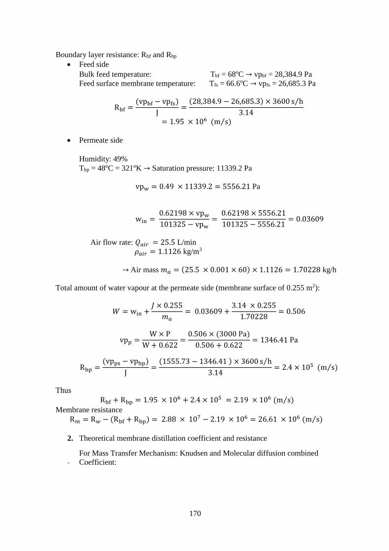
170
Boundary layer resistance: Rbf and Rbp
Feed side
Bulk feed temperature: Tbf = 68oC → vpbf = 28,384.9 Pa
Feed surface membrane temperature: Tfs = 66.6oC → vpfs = 26,685.3 Pa
Rbf =(vpbf − vpfs)
J=
(28,384.9 − 26,685.3) × 3600 s h⁄
3.14= 1.95 × 10⁶ (m s⁄ )
Permeate side
Humidity: 49%
Tbp = 48oC = 321oK → Saturation pressure: 11339.2 Pa
vpw = 0.49 × 11339.2 = 5556.21 Pa
win = 0.62198 × vpw
101325 − vpw=
0.62198 × 5556.21
101325 − 5556.21= 0.03609
Air flow rate: 𝑄𝑎𝑖𝑟 = 25.5 L/min
𝜌𝑎𝑖𝑟 = 1.1126 kg/m3
→ Air mass 𝑚𝑎 = (25.5 × 0.001 × 60) × 1.1126 = 1.70228 kg/h
Total amount of water vapour at the permeate side (membrane surface of 0.255 m2):
𝑊 = win +𝐽 × 0.255
𝑚𝑎= 0.03609 +
3.14 × 0.255
1.70228= 0.506
vpp =W × P
W + 0.622=
0.506 × (3000 Pa)
0.506 + 0.622= 1346.41 Pa
Rbp =(vpps − vpbp)
J=
(1555.73 − 1346.41 ) × 3600 s h⁄
3.14= 2.4 × 10⁵ (m s⁄ )
Thus
Rbf + Rbp = 1.95 × 10⁶ + 2.4 × 105 = 2.19 × 10⁶ (m s⁄ )
Membrane resistance
R𝑚 = R𝑤 − (Rbf + Rbp) = 2.88 × 10⁷ − 2.19 × 106 = 26.61 × 10⁶ (m s⁄ )
2. Theoretical membrane distillation coefficient and resistance
For Mass Transfer Mechanism: Knudsen and Molecular diffusion combined
- Coefficient:
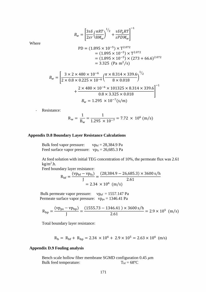
171
𝐵𝑤 = [3𝜏𝛿
2휀𝑟(
𝜋𝑅𝑇
8𝑀𝑤)
12⁄
+𝜏𝛿𝑃𝑎𝑅𝑇
휀𝑃𝐷𝑀𝑤]
−1
Where
PD = (1.895 × 10⁻⁵) × T2.072
= (1.895 × 10⁻⁵) × T2.072
= (1.895 × 10−5) × (273 + 66.6)2.072
= 3.325 (Pa m2 s⁄ )
𝐵𝑤 = [3 × 2 × 480 × 10−6
2 × 0.8 × 0.225 × 10−6(
𝜋 × 8.314 × 339.6
8 × 0.018)
12⁄
+2 × 480 × 10−6 × 101325 × 8.314 × 339.6
0.8 × 3.325 × 0.018]
−1
𝐵𝑤 = 1.295 × 10⁻⁷(s m⁄ )
- Resistance:
Rw = 1
Bw=
1
1.295 × 10−7= 7.72 × 10⁶ (m s⁄ )
Appendix D.8 Boundary Layer Resistance Calculations
Bulk feed vapor pressure: vpbf = 28,384.9 Pa
Feed surface vapor pressure: vpfs = 26,685.3 Pa
At feed solution with initial TEG concentration of 10%, the permeate flux was 2.61
kg/m2.h.
Feed boundary layer resistance:
Rbf =(vpbf − vpfs)
J=
(28,384.9 − 26,685.3) × 3600 s h⁄
2.61= 2.34 × 10⁶ (m s⁄ )
Bulk permeate vapor pressure: vppf = 1557.147 Pa
Permeate surface vapor pressure: vpps = 1346.41 Pa
Rbp =(vpps − vpbp)
J=
(1555.73 − 1346.41 ) × 3600 s h⁄
2.61= 2.9 × 10⁵ (m s⁄ )
Total boundary layer resistance:
Rb = Rbf + Rbp = 2.34 × 10⁶ + 2.9 × 105 = 2.63 × 10⁶ (m/s)
Appendix D.9 Fouling analysis
Bench scale hollow fiber membrane SGMD configuration 0.45 𝜇m
Bulk feed temperature: Tbf = 68oC
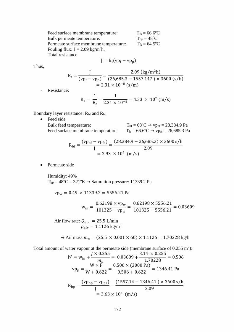
172
Feed surface membrane temperature: Tfs = 66.6oC
Bulk permeate temperature: Tbp = 48oC
Permeate surface membrane temperature: Tfs = 64.5oC
Fouling flux: J = 2.09 kg/m2h.
Total resistance
J = Bt(vpf − vpp)
Thus,
Bt =J
(vpf − vpp)=
2.09 (kg m2h⁄ )
(26,685.3 − 1557.147 ) × 3600 (s h⁄ )
= 2.31 × 10⁻⁸ (s m⁄ )
- Resistance:
R𝑡 = 1
B𝑡=
1
2.31 × 10−8= 4.33 × 10⁷ (m s⁄ )
Boundary layer resistance: Rbf and Rbp
Feed side
Bulk feed temperature: Tbf = 68oC → vpbf = 28,384.9 Pa
Feed surface membrane temperature: Tfs = 66.6oC → vpfs = 26,685.3 Pa
Rbf =(vpbf − vpfs)
J=
(28,384.9 − 26,685.3) × 3600 s h⁄
2.09= 2.93 × 10⁶ (m s⁄ )
Permeate side
Humidity: 49%
Tbp = 48oC = 321oK → Saturation pressure: 11339.2 Pa
vpw = 0.49 × 11339.2 = 5556.21 Pa
win = 0.62198 × vpw
101325 − vpw=
0.62198 × 5556.21
101325 − 5556.21= 0.03609
Air flow rate: 𝑄𝑎𝑖𝑟 = 25.5 L/min
𝜌𝑎𝑖𝑟 = 1.1126 kg/m3
→ Air mass 𝑚𝑎 = (25.5 × 0.001 × 60) × 1.1126 = 1.70228 kg/h
Total amount of water vapour at the permeate side (membrane surface of 0.255 m2):
𝑊 = win +𝐽 × 0.255
𝑚𝑎= 0.03609 +
3.14 × 0.255
1.70228= 0.506
vpp =W × P
W + 0.622=
0.506 × (3000 Pa)
0.506 + 0.622= 1346.41 Pa
Rbp =(vpbp − vpps)
J=
(1557.14 − 1346.41 ) × 3600 s h⁄
2.09= 3.63 × 10⁵ (m s⁄ )
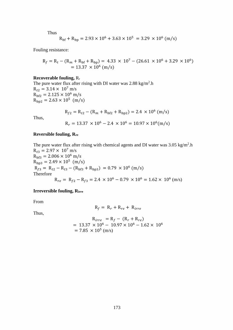
173
Thus
Rbf + Rbp = 2.93 × 10⁶ + 3.63 × 105 = 3.29 × 10⁶ (m s⁄ )
Fouling resistance:
R𝑓 = R𝑡 − (R𝑚 + Rbf + Rbp) = 4.33 × 10⁷ − (26.61 × 10⁶ + 3.29 × 10⁶)
= 13.37 × 10⁶ (m s⁄ )
Recoverable fouling, Rr
The pure water flux after rising with DI water was 2.88 kg/m2.h
R𝑡2 = 3.14 × 10⁷ m/s
Rbf2 = 2.125 × 10⁶ m/s Rbp2 = 2.63 × 10⁵ (m s⁄ )
R𝑓2 = R𝑡2 − (R𝑚 + Rbf2 + Rbp2) = 2.4 × 10⁶ (m s⁄ )
Thus,
R𝑟 = 13.37 × 10⁶ − 2.4 × 106 = 10.97 × 10⁶(m s⁄ )
Reversible fouling, Rre
The pure water flux after rising with chemical agents and DI water was 3.05 kg/m2.h
R𝑡3 = 2.97 × 10⁷ m/s
Rbf3 = 2.006 × 10⁶ m/s Rbp3 = 2.49 × 10⁵ (m s⁄ )
R𝑓3 = R𝑡2 − R𝑡3 − (Rbf3 + Rbp3) = 0.79 × 10⁶ (m s⁄ )
Therefore
R𝑟𝑒 = R𝑓2 − R𝑓3 = 2.4 × 10⁶ − 0.79 × 106 = 1.62 × 10⁶ (m/s)
Irreversible fouling, Rirre
From
R𝑓 = R𝑟 + R𝑟𝑒 + R𝑖𝑟𝑟𝑒
Thus,
R𝑖𝑟𝑟𝑒 = R𝑓 − (R𝑟 + R𝑟𝑒)
= 13.37 × 10⁶ − 10.97 × 10⁶ − 1.62 × 106
= 7.85 × 10⁵ (m/s)

174
Appendix E
Experimental Results
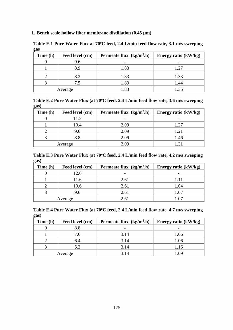
175
1. Bench scale hollow fiber membrane distillation (0.45 µm)
Table E.1 Pure Water Flux at 70oC feed, 2.4 L/min feed flow rate, 3.1 m/s sweeping
gas
Time (h) Feed level (cm) Permeate flux (kg/m2.h) Energy ratio (kW/kg)
0 9.6 - -
1 8.9 1.83 1.27
2 8.2 1.83 1.33
3 7.5 1.83 1.44
Average 1.83 1.35
Table E.2 Pure Water Flux (at 70oC feed, 2.4 L/min feed flow rate, 3.6 m/s sweeping
gas)
Time (h) Feed level (cm) Permeate flux (kg/m2.h) Energy ratio (kW/kg)
0 11.2 - -
1 10.4 2.09 1.27
2 9.6 2.09 1.21
3 8.8 2.09 1.46
Average 2.09 1.31
Table E.3 Pure Water Flux (at 70oC feed, 2.4 L/min feed flow rate, 4.2 m/s sweeping
gas)
Time (h) Feed level (cm) Permeate flux (kg/m2.h) Energy ratio (kW/kg)
0 12.6 - -
1 11.6 2.61 1.11
2 10.6 2.61 1.04
3 9.6 2.61 1.07
Average 2.61 1.07
Table E.4 Pure Water Flux (at 70oC feed, 2.4 L/min feed flow rate, 4.7 m/s sweeping
gas)
Time (h) Feed level (cm) Permeate flux (kg/m2.h) Energy ratio (kW/kg)
0 8.8 - -
1 7.6 3.14 1.06
2 6.4 3.14 1.06
3 5.2 3.14 1.16
Average 3.14 1.09

176
Table E.5 Pure Water Flux (at 70oC feed, 2.4 L/min feed flow rate, 5.3 m/s sweeping
gas)
Time (h) Feed level (cm) Permeate flux (kg/m2.h) Energy ratio (kW/kg)
0 15.7 - -
1 14.7 2.61 1.59
2 13.6 2.88 1.06
3 12.6 2.61 1.24
Average 2.70 1.30
Table E.6 Pure Water Flux (at 60oC feed, 2.4 L/min feed flow rate, 3.1 m/s sweeping
gas)
Time (h) Feed level (cm) Permeate flux (kg/m2.h) Energy ratio (kW/kg)
0 17.9 - -
1 17.4 1.31 1.39
2 16.9 1.31 1.39
3 16.4 1.31 1.42
Average 1.31 1.40
Table E.7 Pure Water Flux (at 60oC feed, 2.4 L/min feed flow rate, 3.6 m/s sweeping
gas)
Time (h) Feed level (cm) Permeate flux (kg/m2.h) Energy ratio (kW/kg)
0 16.4 - -
1 15.8 1.57 1.37
2 15.2 1.57 1.17
3 14.6 1.57 1.29
Average 1.57 1.27
Table E.8 Pure Water Flux (at 60oC feed, 2.4 L/min feed flow rate, 4.2 m/s sweeping
gas)
Time (h) Feed level (cm) Permeate flux (kg/m2.h) Energy ratio (kW/kg)
0 14.6 - -
1 13.9 1.83 1.46
2 13.2 1.83 1.24
3 12.5 1.83 1.31
Average 1.83 1.34
Table E.9 Pure Water Flux (at 60oC feed, 2.4 L/min feed flow rate, 4.7 m/s sweeping
gas)
Time (h) Feed level (cm) Permeate flux (kg/m2.h) Energy ratio (kW/kg)
0 13.2 - -
1 12.5 2.09 1.35
2 11.8 1.83 1.42
3 0 1.83 0.63
Average 1.92 1.13
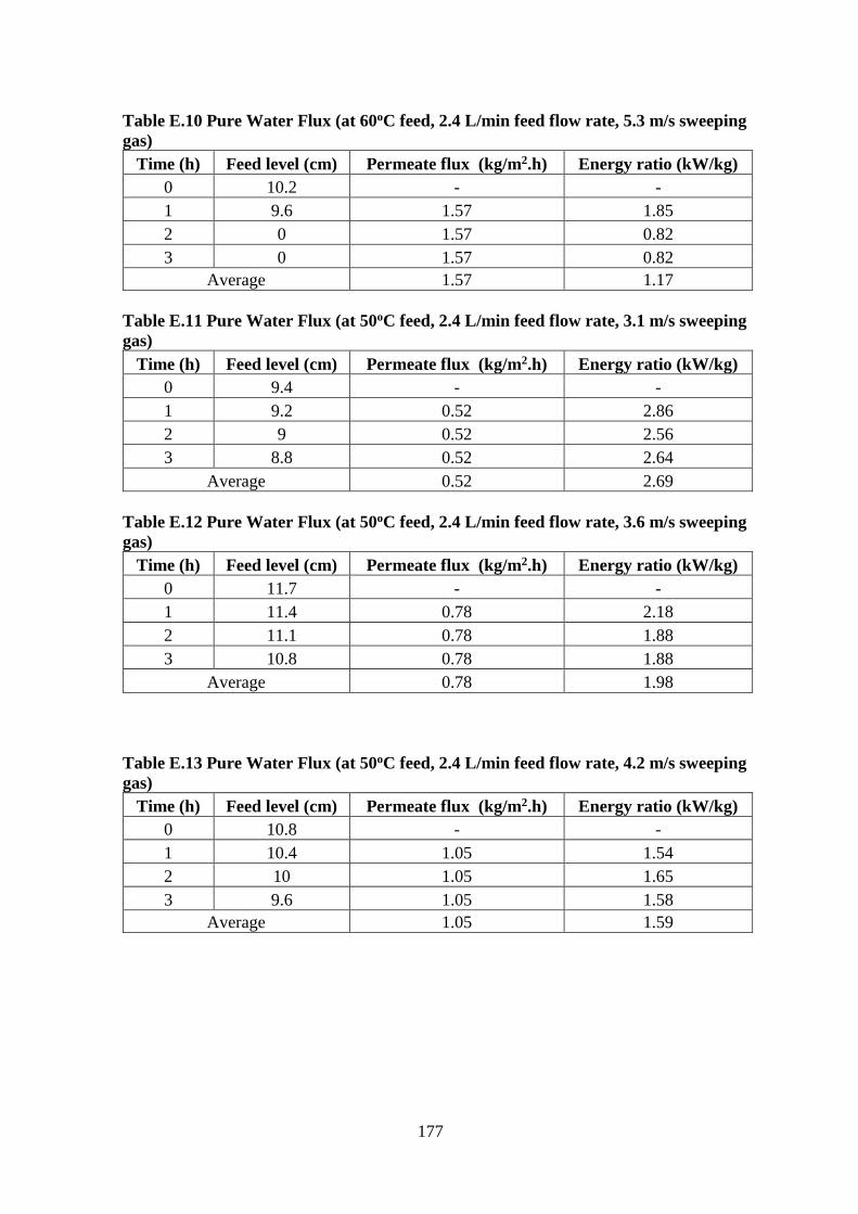
177
Table E.10 Pure Water Flux (at 60oC feed, 2.4 L/min feed flow rate, 5.3 m/s sweeping
gas)
Time (h) Feed level (cm) Permeate flux (kg/m2.h) Energy ratio (kW/kg)
0 10.2 - -
1 9.6 1.57 1.85
2 0 1.57 0.82
3 0 1.57 0.82
Average 1.57 1.17
Table E.11 Pure Water Flux (at 50oC feed, 2.4 L/min feed flow rate, 3.1 m/s sweeping
gas)
Time (h) Feed level (cm) Permeate flux (kg/m2.h) Energy ratio (kW/kg)
0 9.4 - -
1 9.2 0.52 2.86
2 9 0.52 2.56
3 8.8 0.52 2.64
Average 0.52 2.69
Table E.12 Pure Water Flux (at 50oC feed, 2.4 L/min feed flow rate, 3.6 m/s sweeping
gas)
Time (h) Feed level (cm) Permeate flux (kg/m2.h) Energy ratio (kW/kg)
0 11.7 - -
1 11.4 0.78 2.18
2 11.1 0.78 1.88
3 10.8 0.78 1.88
Average 0.78 1.98
Table E.13 Pure Water Flux (at 50oC feed, 2.4 L/min feed flow rate, 4.2 m/s sweeping
gas)
Time (h) Feed level (cm) Permeate flux (kg/m2.h) Energy ratio (kW/kg)
0 10.8 - -
1 10.4 1.05 1.54
2 10 1.05 1.65
3 9.6 1.05 1.58
Average 1.05 1.59

178
Table E.14 Pure Water Flux (at 50oC feed, 2.4 L/min feed flow rate, 4.7 m/s sweeping
gas)
Time (h) Feed level (cm) Permeate flux (kg/m2.h) Energy ratio (kW/kg)
0 9.6 - -
1 9.2 1.05 1.78
2 8.8 1.05 1.89
3 8.4 1.05 1.11
Average 1.05 1.59
Table E.15 Pure Water Flux (at 50oC feed, 2.4 L/min feed flow rate, 5.3 m/s sweeping
gas)
Time (h) Feed level (cm) Permeate flux (kg/m2.h) Energy ratio (kW/kg)
0 8.4 - -
1 8 1.05 1.99
2 7.6 1.05 1.24
3 7.2 1.05 1.24
Average 1.05 1.49
Table E.16 Pure Water Flux (at 70oC feed, 2 L/min feed flow rate, 3.1 m/s sweeping
gas)
Time (h) Feed level (cm) Permeate flux (kg/m2.h) Energy ratio (kW/kg)
0 9.6 - -
1 8.9 1.83 1.38
2 8.2 1.83 1.50
3 7.5 1.83 1.42
Average 1.83 1.43
Table E.17 Pure Water Flux (at 70oC feed, 2 L/min feed flow rate, 3.6 m/s sweeping
gas)
Time (h) Feed level (cm) Permeate flux (kg/m2.h) Energy ratio (kW/kg)
0 14.9 - -
1 14.1 2.09 1.29
2 13.25 2.22 1.21
3 12.5 1.96 1.43
Average 2.09 1.31

179
Table E.18 Pure Water Flux (at 70oC feed, 2 L/min feed flow rate, 4.2 m/s sweeping
gas)
Time (h) Feed level (cm) Permeate flux (kg/m2.h) Energy ratio (kW/kg)
0 12 - -
1 11 2.61 1.13
2 10 2.61 1.23
3 9 2.61 1.13
Average 2.61 1.16
Table E.19 Pure Water Flux (at 70oC feed, 2 L/min feed flow rate, 4.7 m/s sweeping
gas)
Time (h) Feed level (cm) Permeate flux (kg/m2.h) Energy ratio (kW/kg)
0 11.7 - -
1 10.65 2.75 1.22
2 9.5 3.01 1.02
3 8.45 2.75 1.31
Average 2.83 1.18
Table E.20 Pure Water Flux (at 70oC feed, 2 L/min feed flow rate, 5.3 m/s sweeping
gas)
Time (h) Feed level (cm) Permeate flux (kg/m2.h) Energy ratio (kW/kg)
0 16.9 - -
1 16 2.35 1.48
2 15.1 2.35 1.37
3 14.2 2.35 1.58
Average 2.35 1.42
Table E.21 Pure Water Flux (at 60oC feed, 2 L/min feed flow rate, 3.1 m/s sweeping
gas)
Time (h) Feed level (cm) Permeate flux (kg/m2.h) Energy ratio (kW/kg)
0 11.1 - -
1 10.6 1.31 1.27
2 10.1 1.31 1.39
3 9.6 1.31 1.33
Average 1.31 1.33
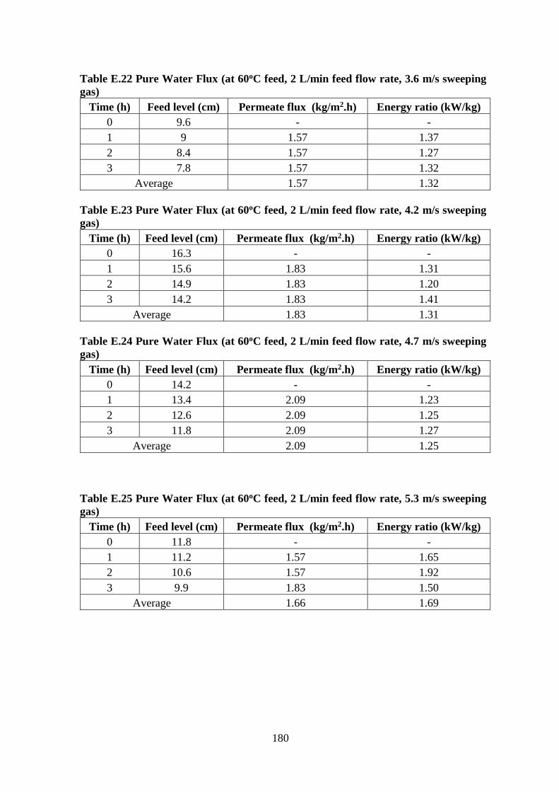
180
Table E.22 Pure Water Flux (at 60oC feed, 2 L/min feed flow rate, 3.6 m/s sweeping
gas)
Time (h) Feed level (cm) Permeate flux (kg/m2.h) Energy ratio (kW/kg)
0 9.6 - -
1 9 1.57 1.37
2 8.4 1.57 1.27
3 7.8 1.57 1.32
Average 1.57 1.32
Table E.23 Pure Water Flux (at 60oC feed, 2 L/min feed flow rate, 4.2 m/s sweeping
gas)
Time (h) Feed level (cm) Permeate flux (kg/m2.h) Energy ratio (kW/kg)
0 16.3 - -
1 15.6 1.83 1.31
2 14.9 1.83 1.20
3 14.2 1.83 1.41
Average 1.83 1.31
Table E.24 Pure Water Flux (at 60oC feed, 2 L/min feed flow rate, 4.7 m/s sweeping
gas)
Time (h) Feed level (cm) Permeate flux (kg/m2.h) Energy ratio (kW/kg)
0 14.2 - -
1 13.4 2.09 1.23
2 12.6 2.09 1.25
3 11.8 2.09 1.27
Average 2.09 1.25
Table E.25 Pure Water Flux (at 60oC feed, 2 L/min feed flow rate, 5.3 m/s sweeping
gas)
Time (h) Feed level (cm) Permeate flux (kg/m2.h) Energy ratio (kW/kg)
0 11.8 - -
1 11.2 1.57 1.65
2 10.6 1.57 1.92
3 9.9 1.83 1.50
Average 1.66 1.69

181
Table E.26 Pure Water Flux (at 50oC feed, 2 L/min feed flow rate, 3.1 m/s sweeping
gas)
Time (h) Feed level (cm) Permeate flux (kg/m2.h) Energy ratio (kW/kg)
0 15.1 - -
1 14.9 0.52 2.56
2 14.7 0.52 2.56
3 14.5 0.52 2.56
Average 0.52 2.56
Table E.27 Pure Water Flux (at 50oC feed, 2 L/min feed flow rate, 3.6 m/s sweeping
gas)
Time (h) Feed level (cm) Permeate flux (kg/m2.h) Energy ratio (kW/kg)
0 14.3 - -
1 14 0.78 1.93
2 13.7 0.78 1.88
3 13.4 0.78 1.88
Average 0.78 1.90
Table E.28 Pure Water Flux (at 50oC feed, 2 L/min feed flow rate, 4.2 m/s sweeping
gas)
Time (h) Feed level (cm) Permeate flux (kg/m2.h) Energy ratio (kW/kg)
0 13.3 - -
1 12.9 1.05 1.58
2 12.5 1.05 1.61
3 12.1 1.05 1.54
Average 1.05 1.58
Table E.29 Pure Water Flux (at 50oC feed, 2 L/min feed flow rate, 4.7 m/s sweeping
gas)
Time (h) Feed level (cm) Permeate flux (kg/m2.h) Energy ratio (kW/kg)
0 11.5 - -
1 11.1 1.05 1.86
2 10.7 1.05 1.74
3 10.3 1.05 1.74
Average 1.05 1.78

182
Table E.30 Pure Water Flux (at 50oC feed, 2 L/min feed flow rate, 5.3 m/s sweeping
gas)
Time (h) Feed level (cm) Permeate flux (kg/m2.h) Energy ratio (kW/kg)
0 10.5 - -
1 10.1 1.05 2.02
2 9.7 1.05 1.95
3 9.3 1.05 2.14
Average 1.05 2.04
Table E.31 Pure Water Flux (at 50oC feed, 1.6 L/min feed flow rate, 3.1 m/s sweeping
gas)
Time (h) Feed level (cm) Permeate flux (kg/m2.h) Energy ratio (kW/kg)
0 15.6 - -
1 14.9 1.83 1.40
2 14.2 1.83 1.33
3 13.7 1.31 1.84
Average 1.66 1.52
Table E.32 Pure Water Flux (at 70oC feed, 1.6 L/min feed flow rate, 3.6 m/s sweeping
gas)
Time (h) Feed level (cm) Permeate flux (kg/m2.h) Energy ratio (kW/kg)
0 13.5 - -
1 12.7 2.09 1.23
2 11.9 2.09 1.21
3 11.1 2.09 1.29
Average 2.09 1.24
Table E.33 Pure Water Flux (at 70oC feed, 1.6 L/min feed flow rate, 4.2 m/s sweeping
gas)
Time (h) Feed level (cm) Permeate flux (kg/m2.h) Energy ratio (kW/kg)
0 10.4 - -
1 9.5 2.35 1.18
2 8.5 2.61 1.14
3 7.6 2.35 1.32
Average 2.44 1.21
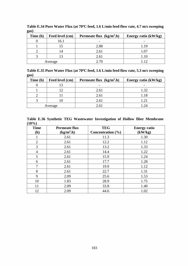
183
Table E.34 Pure Water Flux (at 70oC feed, 1.6 L/min feed flow rate, 4.7 m/s sweeping
gas)
Time (h) Feed level (cm) Permeate flux (kg/m2.h) Energy ratio (kW/kg)
0 16.1 - -
1 15 2.88 1.19
2 14 2.61 1.07
3 13 2.61 1.10
Average 2.70 1.12
Table E.35 Pure Water Flux (at 70oC feed, 1.6 L/min feed flow rate, 5.3 m/s sweeping
gas)
Time (h) Feed level (cm) Permeate flux (kg/m2.h) Energy ratio (kW/kg)
0 13 - -
1 12 2.61 1.32
2 11 2.61 1.18
3 10 2.61 1.21
Average 2.61 1.24
Table E.36 Synthetic TEG Wastewater Investigation of Hollow fiber Membrane
(10%)
Time
(h)
Permeate flux
(kg/m2.h)
TEG
Concentration (%)
Energy ratio
(kW/kg)
1 2.61 11.3 1.30
2 2.61 12.2 1.12
3 2.61 13.2 1.33
4 2.61 14.4 1.22
5 2.61 15.9 1.24
6 2.61 17.7 1.28
7 2.61 19.9 1.12
8 2.61 22.7 1.31
9 2.09 25.6 1.53
10 1.83 28.9 1.75
11 2.09 33.8 1.40
12 2.09 44.6 1.02

184
Table E.37 Synthetic TEG Wastewater Investigation of Hollow fiber Membrane
(30%)
Time
(h)
Permeate flux
(kg/m2.h)
TEG Concentration
(%)
Energy ratio
(kW/kg)
1 1.57 32.6 2.11
2 2.09 33.1 1.38
3 1.83 34.9 1.79
4 2.09 37.2 1.42
5 2.35 40.2 1.36
6 2.09 43.3 1.32
7 1.83 46.4 1.64
8 2.09 50.6 1.38
9 2.09 55.6 1.42
10 1.31 59.2 2.17
12 1.57 60.4 1.86
Table E.38 Synthetic TEG Wastewater Investigation of Hollow fiber Membrane
(60%)
Time
(h)
Permeate flux
(kg/m2.h)
TEG Concentration
(%)
Energy ratio
(kW/kg)
1 0.52 60.8 4.76
2 1.05 62.5 2.72
3 1.05 64.3 2.38
4 1.05 66.2 2.46
5 1.05 68.2 2.42
6 1.05 70.3 2.38
7 0.78 72.0 2.92
8 0.78 73.8 3.12
9 0.52 75.0 4.69
11 0.52 77.6 3.21
12 0.52 78.9 4.46
13 0.52 80.4 4.24
23 0.00 90.5 4.41
Table E.39 Continuously-fed Synthetic TEG Wastewater Investigation of Hollow
fiber Membrane
Time
(h)
Permeate flux
(kg/m2.h)
TEG Concentration
(%)
Energy ratio
(kW/kg)
1 2.61 10.7 1.13
2 2.61 11.2 1.06
3 2.61 12.1 1.43
4 2.61 13.2 1.30
5 2.61 14.5 1.27
6 2.61 16.2 1.28
7 2.61 18.2 1.21
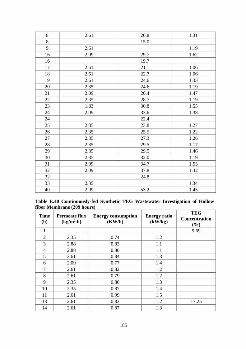
185
8 2.61 20.8 1.31
8 15.0
9 2.61 1.19
16 2.09 29.7 1.62
16 19.7
17 2.61 21.1 1.06
18 2.61 22.7 1.06
19 2.61 24.6 1.33
20 2.35 24.6 1.19
21 2.09 26.4 1.47
22 2.35 28.7 1.19
23 1.83 30.8 1.55
24 2.09 33.6 1.38
24 22.4
25 2.35 23.8 1.27
26 2.35 25.5 1.22
27 2.35 27.3 1.26
28 2.35 29.5 1.17
29 2.35 29.5 1.46
30 2.35 32.0 1.19
31 2.09 34.7 1.53
32 2.09 37.8 1.32
32 24.8
33 2.35 1.34
40 2.09 53.2 1.45
Table E.40 Continuously-fed Synthetic TEG Wastewater Investigation of Hollow
fiber Membrane (209 hours)
Time
(h)
Permeate flux
(kg/m2.h)
Energy consumption
(KW/h)
Energy ratio
(kW/kg)
TEG
Concentration
(%)
1 9.69
2 2.35 0.74 1.2
3 2.88 0.83 1.1
4 2.88 0.80 1.1
5 2.61 0.84 1.3
6 2.09 0.77 1.4
7 2.61 0.82 1.2
8 2.61 0.79 1.2
9 2.35 0.80 1.3
10 2.35 0.87 1.4
11 2.61 0.99 1.5
13 2.61 0.82 1.2 17.25
14 2.61 0.87 1.3
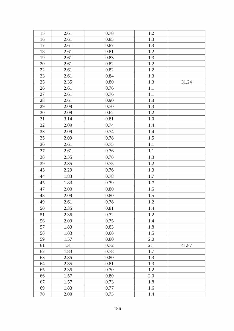
186
15 2.61 0.78 1.2
16 2.61 0.85 1.3
17 2.61 0.87 1.3
18 2.61 0.81 1.2
19 2.61 0.83 1.3
20 2.61 0.82 1.2
22 2.61 0.82 1.2
23 2.61 0.84 1.3
25 2.35 0.80 1.3 31.24
26 2.61 0.76 1.1
27 2.61 0.76 1.1
28 2.61 0.90 1.3
29 2.09 0.70 1.3
30 2.09 0.62 1.2
31 3.14 0.81 1.0
32 2.09 0.74 1.4
33 2.09 0.74 1.4
35 2.09 0.78 1.5
36 2.61 0.75 1.1
37 2.61 0.76 1.1
38 2.35 0.78 1.3
39 2.35 0.75 1.2
43 2.29 0.76 1.3
44 1.83 0.78 1.7
45 1.83 0.79 1.7
47 2.09 0.80 1.5
48 2.09 0.80 1.5
49 2.61 0.78 1.2
50 2.35 0.81 1.4
51 2.35 0.72 1.2
56 2.09 0.75 1.4
57 1.83 0.83 1.8
58 1.83 0.68 1.5
59 1.57 0.80 2.0
61 1.31 0.72 2.1 41.87
62 1.83 0.78 1.7
63 2.35 0.80 1.3
64 2.35 0.81 1.3
65 2.35 0.70 1.2
66 1.57 0.80 2.0
67 1.57 0.73 1.8
69 1.83 0.77 1.6
70 2.09 0.73 1.4

187
71 2.09 0.65 1.2
80 1.96 0.79 1.6 56.24
81 1.57 0.60 1.5
82 1.31 0.66 2.0
83 1.31 0.60 1.8
84 1.05 0.62 2.3
85 1.57 0.66 1.7
87 1.83 0.63 1.3
88 1.83 0.83 1.8
90 1.83 0.73 1.6
92 1.83 0.66 1.4
93 1.57 0.79 2.0
95 2.09 0.80 1.5 71.18
106 1.38 0.66 1.9
107 1.31 0.65 1.9
108 1.31 0.63 1.9
109 1.05 0.58 2.2
111 0.65 0.59 3.6
112 0.78 0.58 2.9
113 0.26 0.53 7.9
115 2.09 0.79 1.5
116 1.83 0.69 1.5
118 1.70 0.73 1.7
131 1.15 0.64 2.2
132 0.26 0.64 9.7
133 0.52 0.60 4.5
135 2.09 0.67 1.3 77.38
136 1.05 0.64 2.4
137 2.09 0.68 1.3
155 1.00 0.62 2.4
156 0.13 0.69 20.5
158 2.09 0.66 1.2 98.01
160 1.57 0.67 1.7
161 1.31 0.66 2.0
162 2.35 0.93 1.6
163 1.57 0.69 1.7
165 1.05 0.66 2.5
176 0.76 0.63 3.3
177 0.26 0.41 6.2
178 0.26 0.51 7.6
179 0.26 0.47 7.0
180 0.26 0.49 7.4
182 1.57 0.63 1.6
183 1.57 0.66 1.7
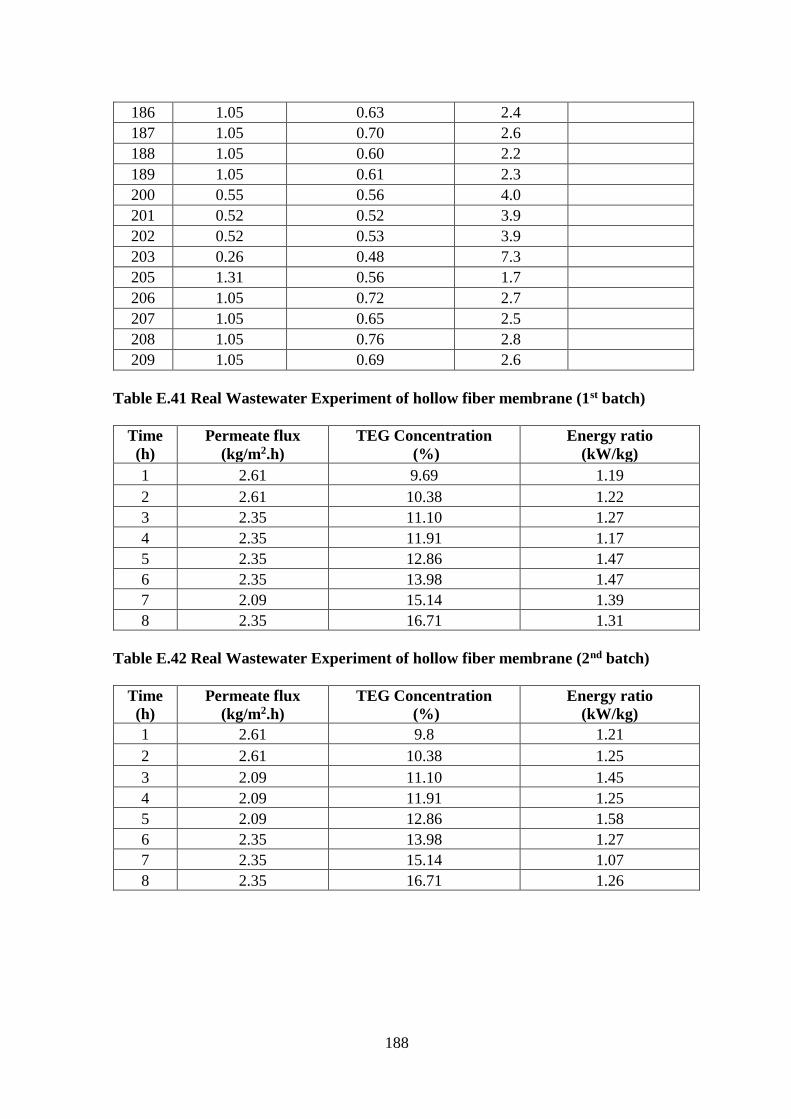
188
186 1.05 0.63 2.4
187 1.05 0.70 2.6
188 1.05 0.60 2.2
189 1.05 0.61 2.3
200 0.55 0.56 4.0
201 0.52 0.52 3.9
202 0.52 0.53 3.9
203 0.26 0.48 7.3
205 1.31 0.56 1.7
206 1.05 0.72 2.7
207 1.05 0.65 2.5
208 1.05 0.76 2.8
209 1.05 0.69 2.6
Table E.41 Real Wastewater Experiment of hollow fiber membrane (1st batch)
Time
(h)
Permeate flux
(kg/m2.h)
TEG Concentration
(%)
Energy ratio
(kW/kg)
1 2.61 9.69 1.19
2 2.61 10.38 1.22
3 2.35 11.10 1.27
4 2.35 11.91 1.17
5 2.35 12.86 1.47
6 2.35 13.98 1.47
7 2.09 15.14 1.39
8 2.35 16.71 1.31
Table E.42 Real Wastewater Experiment of hollow fiber membrane (2nd batch)
Time
(h)
Permeate flux
(kg/m2.h)
TEG Concentration
(%)
Energy ratio
(kW/kg)
1 2.61 9.8 1.21
2 2.61 10.38 1.25
3 2.09 11.10 1.45
4 2.09 11.91 1.25
5 2.09 12.86 1.58
6 2.35 13.98 1.27
7 2.35 15.14 1.07
8 2.35 16.71 1.26

189
Table E.43 Real Wastewater Experiment of hollow fiber membrane (3rd batch)
Time
(h)
Permeate flux
(kg/m2.h)
TEG Concentration
(%)
Energy ratio
(kW/kg)
1 2.61 9.70 1.29
2 2.35 10.31 1.30
3 2.35 11.01 1.40
4 2.35 11.82 1.20
5 2.35 12.75 1.20
6 2.35 13.84 1.30
7 2.35 15.14 1.20
8 2.35 16.71 1.30
Table E.44 Real Wastewater Experiment of hollow fiber membrane (4th batch)
Time
(h)
Permeate flux
(kg/m2.h)
TEG Concentration
(%)
Energy ratio
(kW/kg)
1 2.35 9.69 1.25
2 2.35 10.31 1.30
3 2.35 11.01 1.30
4 2.35 11.82 1.30
5 2.35 12.75 1.20
6 2.35 13.84 1.30
7 2.35 15.14 1.20
8 2.09 16.52 1.30
Table E.45 Real Wastewater Experiment of hollow fiber membrane (5th batch)
Time
(h)
Permeate flux
(kg/m2.h)
TEG Concentration
(%)
Energy ratio
(kW/kg)
1 2.35 9.69 1.29
2 2.35 10.31 1.3
3 2.35 11.01 1.3
4 2.35 11.82 1.3
5 2.35 12.75 1.2
6 2.35 13.84 1.3
7 2.09 14.98 1.4
8 2.09 16.33 2.3
Table E.46 Real Wastewater Experiment of hollow fiber membrane (40 hours)
Time
(h)
Permeate flux
(kg/m2.h)
TEG Concentration
(%)
Energy ratio
(kW/kg)
0 - 9.69 -
1 2.35 1.2
7 - 16.90 -
8 2.09 25.13 1.3
8 - 20.23 -
9 2.35 21.52 1.1
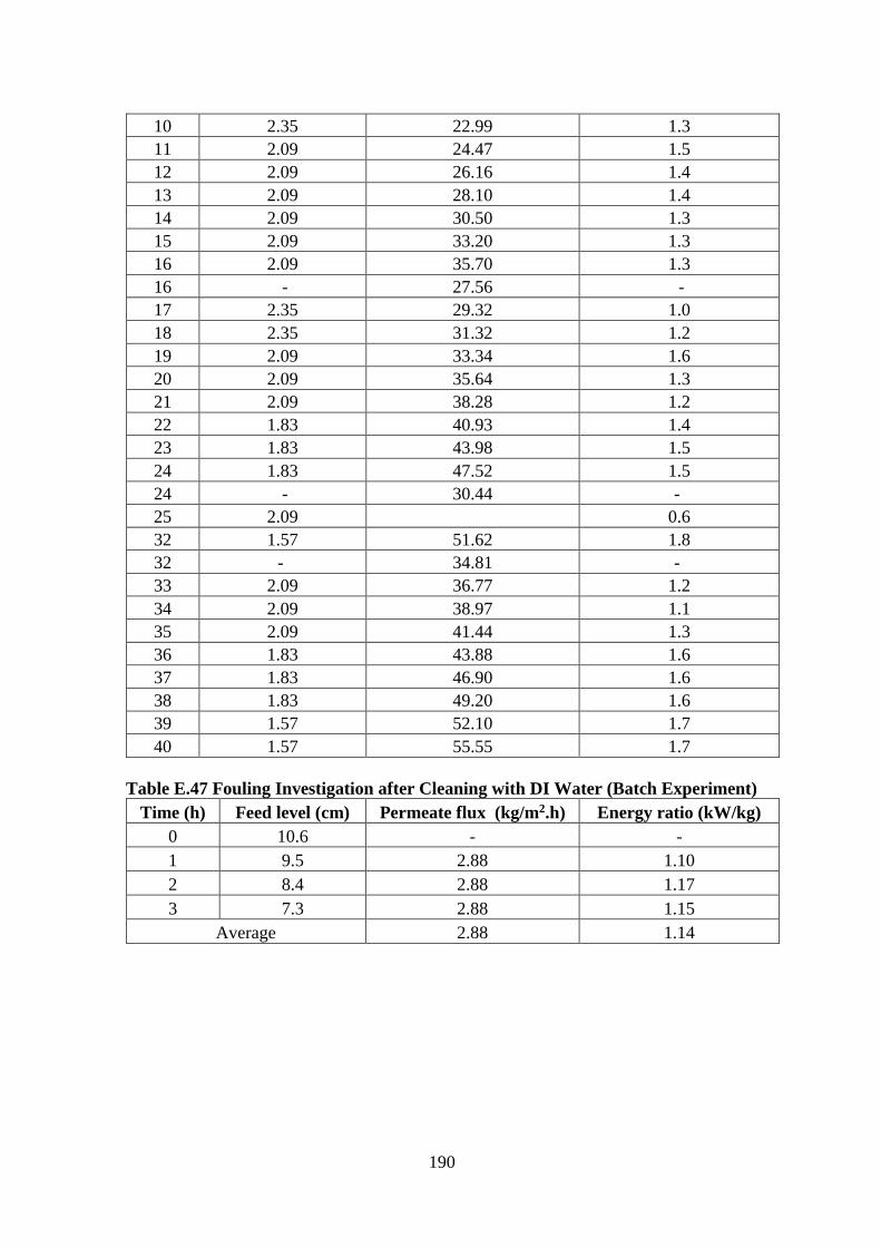
190
10 2.35 22.99 1.3
11 2.09 24.47 1.5
12 2.09 26.16 1.4
13 2.09 28.10 1.4
14 2.09 30.50 1.3
15 2.09 33.20 1.3
16 2.09 35.70 1.3
16 - 27.56 -
17 2.35 29.32 1.0
18 2.35 31.32 1.2
19 2.09 33.34 1.6
20 2.09 35.64 1.3
21 2.09 38.28 1.2
22 1.83 40.93 1.4
23 1.83 43.98 1.5
24 1.83 47.52 1.5
24 - 30.44 -
25 2.09 0.6
32 1.57 51.62 1.8
32 - 34.81 -
33 2.09 36.77 1.2
34 2.09 38.97 1.1
35 2.09 41.44 1.3
36 1.83 43.88 1.6
37 1.83 46.90 1.6
38 1.83 49.20 1.6
39 1.57 52.10 1.7
40 1.57 55.55 1.7
Table E.47 Fouling Investigation after Cleaning with DI Water (Batch Experiment)
Time (h) Feed level (cm) Permeate flux (kg/m2.h) Energy ratio (kW/kg)
0 10.6 - -
1 9.5 2.88 1.10
2 8.4 2.88 1.17
3 7.3 2.88 1.15
Average 2.88 1.14

191
Table E.48 Fouling Investigation after Cleaning with Chemical Agents (Batch
Experiment)
Time (h) Feed level (cm) Permeate flux (kg/m2.h) Energy ratio (kW/kg)
0 9 - -
1 7.8 3.14 1.06
2 6.6 3.14 0.94
3 5.5 2.88 1.23
Average 3.05 1.08
Table E.49 Fouling Investigation after Cleaning with DI Water (Continuously-fed
Experiment)
Time (h) Feed level (cm) Permeate flux (kg/m2.h) Energy ratio (kW/kg)
0 13.7 - -
1 12.6 2.88
1.15
2 11.5 2.88
3 10.4 2.88
Average 2.88 1.15
Table E.49 Fouling Investigation after Cleaning with Chemical Agents (Continuously-
fed Experiment)
Time (h) Feed level (cm) Permeate flux (kg/m2.h) Energy ratio (kW/kg)
0 15.3 - -
1 14.1 3.14 1.01
2 12.9 3.14 1.06
3 11.8 2.88 1.18
Average 3.05 1.08
2. Pilot Scale Study
Table E.51 Pure Water Flux Investigation (feed flow rate 60 L/min, feed temperature
70oC)
Sweeping
Gas Inlet
Velocity
(m/s)
First Experiment
Duplicated
Experiment Average
Permeate
flux
(kg/m2.h)
Energy
ratio
(kW/kg)
Permeate
flux
(kg/m2.h)
Energy
ratio
(kW/kg)
Permeate
flux
(kg/m2.h)
Energy
ratio
(kW/kg)
4.29 1 0.586 0.95 0.577 0.98 0.58
4.98 1.19 0.552 1.19 0.541 1.19 0.55
5.25 1.55 0.456 1.51 0.460 1.53 0.46
6.06 1.59 0.486 1.66 0.465 1.63 0.48
6.76 1.75 0.495 1.83 0.459 1.79 0.48
7.57 1.75 0.548 1.89 0.493 1.82 0.52
8.07 1.91 0.518 1.97 0.502 1.94 0.51
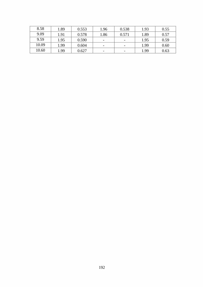
192
8.58 1.89 0.553 1.96 0.538 1.93 0.55
9.09 1.91 0.578 1.86 0.571 1.89 0.57
9.59 1.95 0.590 - - 1.95 0.59
10.09 1.99 0.604 - - 1.99 0.60
10.60 1.99 0.627 - - 1.99 0.63
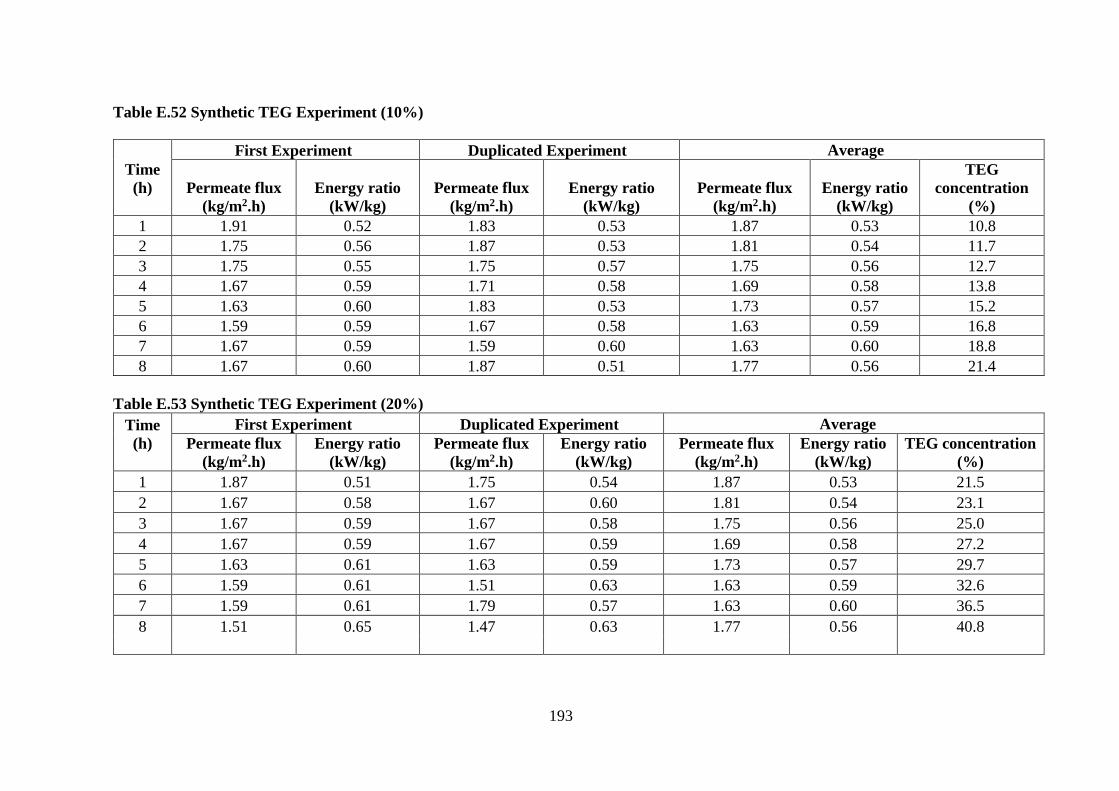
193
Table E.52 Synthetic TEG Experiment (10%)
Time
(h)
First Experiment Duplicated Experiment Average
Permeate flux
(kg/m2.h)
Energy ratio
(kW/kg)
Permeate flux
(kg/m2.h)
Energy ratio
(kW/kg)
Permeate flux
(kg/m2.h)
Energy ratio
(kW/kg)
TEG
concentration
(%)
1 1.91 0.52 1.83 0.53 1.87 0.53 10.8
2 1.75 0.56 1.87 0.53 1.81 0.54 11.7
3 1.75 0.55 1.75 0.57 1.75 0.56 12.7
4 1.67 0.59 1.71 0.58 1.69 0.58 13.8
5 1.63 0.60 1.83 0.53 1.73 0.57 15.2
6 1.59 0.59 1.67 0.58 1.63 0.59 16.8
7 1.67 0.59 1.59 0.60 1.63 0.60 18.8
8 1.67 0.60 1.87 0.51 1.77 0.56 21.4
Table E.53 Synthetic TEG Experiment (20%)
Time
(h)
First Experiment Duplicated Experiment Average
Permeate flux
(kg/m2.h)
Energy ratio
(kW/kg)
Permeate flux
(kg/m2.h)
Energy ratio
(kW/kg)
Permeate flux
(kg/m2.h)
Energy ratio
(kW/kg)
TEG concentration
(%)
1 1.87 0.51 1.75 0.54 1.87 0.53 21.5
2 1.67 0.58 1.67 0.60 1.81 0.54 23.1
3 1.67 0.59 1.67 0.58 1.75 0.56 25.0
4 1.67 0.59 1.67 0.59 1.69 0.58 27.2
5 1.63 0.61 1.63 0.59 1.73 0.57 29.7
6 1.59 0.61 1.51 0.63 1.63 0.59 32.6
7 1.59 0.61 1.79 0.57 1.63 0.60 36.5
8 1.51 0.65 1.47 0.63 1.77 0.56 40.8
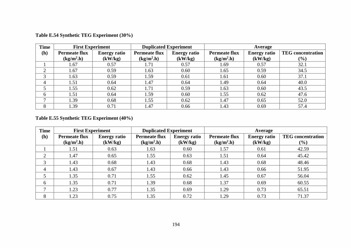
194
Table E.54 Synthetic TEG Experiment (30%)
Time
(h)
First Experiment Duplicated Experiment Average
Permeate flux
(kg/m2.h)
Energy ratio
(kW/kg)
Permeate flux
(kg/m2.h)
Energy ratio
(kW/kg)
Permeate flux
(kg/m2.h)
Energy ratio
(kW/kg)
TEG concentration
(%)
1 1.67 0.57 1.71 0.57 1.69 0.57 32.1
2 1.67 0.59 1.63 0.60 1.65 0.59 34.5
3 1.63 0.59 1.59 0.61 1.61 0.60 37.1
4 1.51 0.64 1.47 0.64 1.49 0.64 40.0
5 1.55 0.62 1.71 0.59 1.63 0.60 43.5
6 1.51 0.64 1.59 0.60 1.55 0.62 47.6
7 1.39 0.68 1.55 0.62 1.47 0.65 52.0
8 1.39 0.71 1.47 0.66 1.43 0.69 57.4
Table E.55 Synthetic TEG Experiment (40%)
Time
(h)
First Experiment Duplicated Experiment Average
Permeate flux
(kg/m2.h)
Energy ratio
(kW/kg)
Permeate flux
(kg/m2.h)
Energy ratio
(kW/kg)
Permeate flux
(kg/m2.h)
Energy ratio
(kW/kg)
TEG concentration
(%)
1 1.51 0.63 1.63 0.60 1.57 0.61 42.59
2 1.47 0.65 1.55 0.63 1.51 0.64 45.42
3 1.43 0.68 1.43 0.68 1.43 0.68 48.46
4 1.43 0.67 1.43 0.66 1.43 0.66 51.95
5 1.35 0.71 1.55 0.62 1.45 0.67 56.04
6 1.35 0.71 1.39 0.68 1.37 0.69 60.55
7 1.23 0.77 1.35 0.69 1.29 0.73 65.51
8 1.23 0.75 1.35 0.72 1.29 0.73 71.37

195
Table E.56 Synthetic TEG Experiment (60%)
Time
(h)
First Experiment Duplicated Experiment Average
Permeate flux
(kg/m2.h)
Energy ratio
(kW/kg)
Permeate flux
(kg/m2.h)
Energy ratio
(kW/kg)
Permeate flux
(kg/m2.h)
Energy ratio
(kW/kg)
TEG
concentration
(%)
1 1.10 0.86 1.27 0.73 1.19 0.79 62.89
2 1.15 0.83 1.27 0.77 1.21 0.80 66.14
3 1.15 0.82 1.19 0.79 1.17 0.80 69.63
4 0.99 0.94 1.19 0.81 1.09 0.87 73.23
5 0.99 0.94 1.19 0.81 1.09 0.87 77.23
6 0.99 0.94 1.19 0.80 1.09 0.87 81.70
7 0.76 1.22 0.72 1.25 0.74 1.23 84.99
8 0.38 2.48 0.52 1.78 0.45 2.13 88.04
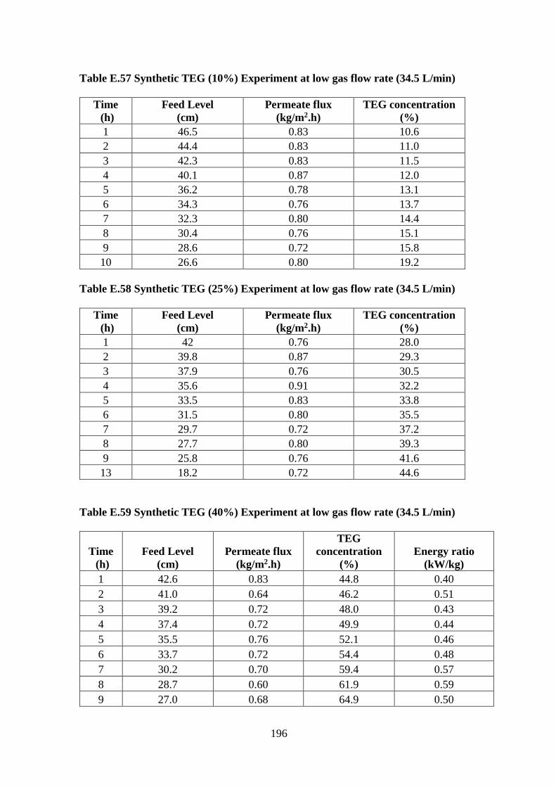
196
Table E.57 Synthetic TEG (10%) Experiment at low gas flow rate (34.5 L/min)
Time
(h)
Feed Level
(cm)
Permeate flux
(kg/m2.h)
TEG concentration
(%)
1 46.5 0.83 10.6
2 44.4 0.83 11.0
3 42.3 0.83 11.5
4 40.1 0.87 12.0
5 36.2 0.78 13.1
6 34.3 0.76 13.7
7 32.3 0.80 14.4
8 30.4 0.76 15.1
9 28.6 0.72 15.8
10 26.6 0.80 19.2
Table E.58 Synthetic TEG (25%) Experiment at low gas flow rate (34.5 L/min)
Time
(h)
Feed Level
(cm)
Permeate flux
(kg/m2.h)
TEG concentration
(%)
1 42 0.76 28.0
2 39.8 0.87 29.3
3 37.9 0.76 30.5
4 35.6 0.91 32.2
5 33.5 0.83 33.8
6 31.5 0.80 35.5
7 29.7 0.72 37.2
8 27.7 0.80 39.3
9 25.8 0.76 41.6
13 18.2 0.72 44.6
Table E.59 Synthetic TEG (40%) Experiment at low gas flow rate (34.5 L/min)
Time
(h)
Feed Level
(cm)
Permeate flux
(kg/m2.h)
TEG
concentration
(%)
Energy ratio
(kW/kg)
1 42.6 0.83 44.8 0.40
2 41.0 0.64 46.2 0.51
3 39.2 0.72 48.0 0.43
4 37.4 0.72 49.9 0.44
5 35.5 0.76 52.1 0.46
6 33.7 0.72 54.4 0.48
7 30.2 0.70 59.4 0.57
8 28.7 0.60 61.9 0.59
9 27.0 0.68 64.9 0.50
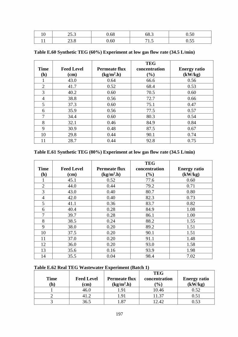
197
10 25.3 0.68 68.3 0.50
11 23.8 0.60 71.5 0.55
Table E.60 Synthetic TEG (60%) Experiment at low gas flow rate (34.5 L/min)
Time
(h)
Feed Level
(cm)
Permeate flux
(kg/m2.h)
TEG
concentration
(%)
Energy ratio
(kW/kg)
1 43.0 0.64 66.6 0.56
2 41.7 0.52 68.4 0.53
3 40.2 0.60 70.5 0.60
4 38.8 0.56 72.7 0.66
5 37.3 0.60 75.1 0.47
6 35.9 0.56 77.5 0.57
7 34.4 0.60 80.3 0.54
8 32.1 0.46 84.9 0.84
9 30.9 0.48 87.5 0.67
10 29.8 0.44 90.1 0.74
11 28.7 0.44 92.8 0.75
Table E.61 Synthetic TEG (80%) Experiment at low gas flow rate (34.5 L/min)
Time
(h)
Feed Level
(cm)
Permeate flux
(kg/m2.h)
TEG
concentration
(%)
Energy ratio
(kW/kg)
1 45.1 0.52 77.6 0.60
2 44.0 0.44 79.2 0.71
3 43.0 0.40 80.7 0.80
4 42.0 0.40 82.3 0.73
5 41.1 0.36 83.7 0.82
6 40.4 0.28 84.9 1.08
7 39.7 0.28 86.1 1.00
8 38.5 0.24 88.2 1.55
9 38.0 0.20 89.2 1.51
10 37.5 0.20 90.1 1.51
11 37.0 0.20 91.1 1.48
12 36.0 0.20 93.0 1.58
13 35.6 0.16 93.9 1.98
14 35.5 0.04 98.4 7.02
Table E.62 Real TEG Wastewater Experiment (Batch 1)
Time
(h)
Feed Level
(cm)
Permeate flux
(kg/m2.h)
TEG
concentration
(%)
Energy ratio
(kW/kg)
1 46.0 1.91 10.46 0.52
2 41.2 1.91 11.37 0.51
3 36.5 1.87 12.42 0.53
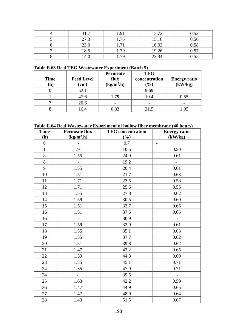
198
4 31.7 1.91 13.72 0.52
5 27.3 1.75 15.18 0.56
6 23.0 1.71 16.93 0.58
7 18.5 1.79 19.26 0.57
8 14.0 1.79 22.34 0.55
Table E.63 Real TEG Wastewater Experiment (Batch 5)
Time
(h)
Feed Level
(cm)
Permeate
flux
(kg/m2.h)
TEG
concentration
(%)
Energy ratio
(kW/kg)
0 52.1 - 9.69
1 47.6 1.79 10.4 0.55
7 20.6 - - -
8 16.4 0.83 21.5 1.05
Table E.64 Real Wastewater Experiment of hollow fiber membrane (40 hours)
Time
(h)
Permeate flux
(kg/m2.h)
TEG concentration
(%)
Energy ratio
(kW/kg)
0 - 9.7 -
1 1.91 10.5 0.50
8 1.55 24.9 0.61
8 - 19.2 -
9 1.55 20.4 0.61
10 1.51 21.7 0.63
11 1.71 23.5 0.58
12 1.71 25.6 0.56
13 1.55 27.8 0.62
14 1.59 30.5 0.60
15 1.51 33.7 0.65
16 1.51 37.5 0.65
16 - 30.9 -
17 1.59 32.9 0.61
18 1.55 35.1 0.63
19 1.55 37.7 0.62
20 1.51 39.8 0.62
21 1.47 42.2 0.65
22 1.39 44.3 0.69
23 1.35 45.1 0.71
24 1.35 47.0 0.71
24 - 39.5 -
25 1.63 42.2 0.59
26 1.47 44.9 0.65
27 1.47 48.0 0.64
28 1.43 51.5 0.67
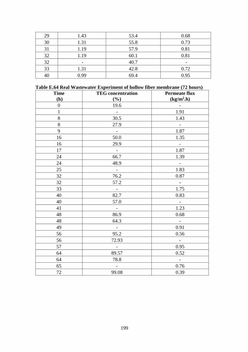
199
29 1.43 53.4 0.68
30 1.31 55.8 0.73
31 1.19 57.9 0.81
32 1.19 60.1 0.81
32 - 40.7 -
33 1.31 42.8 0.72
40 0.99 69.4 0.95
Table E.64 Real Wastewater Experiment of hollow fiber membrane (72 hours)
Time
(h)
TEG concentration
(%)
Permeate flux
(kg/m2.h)
0 19.6 -
1 - 1.91
8 30.5 1.43
8 27.9 -
9 - 1.87
16 50.0 1.35
16 29.9 -
17 - 1.87
24 66.7 1.39
24 48.9 -
25 - 1.83
32 76.2 0.87
32 57.2 -
33 - 1.75
40 82.7 0.83
40 57.0 -
41 - 1.23
48 86.9 0.68
48 64.3 -
49 - 0.91
56 95.2 0.56
56 72.93 -
57 - 0.95
64 89.57 0.52
64 78.8 -
65 - 0.76
72 99.08 0.39

200
Appendix F
Energy Consumption Analysis

201
1. Bench Scale SGMD Introduction
The schematic diagram of bench scale hollow fiber SGMD system is shown in
Figure F.1.
Figure F.1 Bench Scale SGMD System
The equipment that consumed energy of bench scale SGMD system are presented in
Figure F.2
(a) (b) (c) (d)
Figure F.2 Equipment Consume Energy
a. Feed pump b. Heater c. Control box d. Compressor
The energy consumption of electrical heater, feed pump and control box were measured
by a power rotameter
Heater (feed tank)
Model: Seagull - Digital Pro Electric Urn
Company: Thai Stainless Steel Co.,Ltd
Max capacity: 14 L
Permeate tank
Heater
Feed
tank Gas Compressor
MD Module
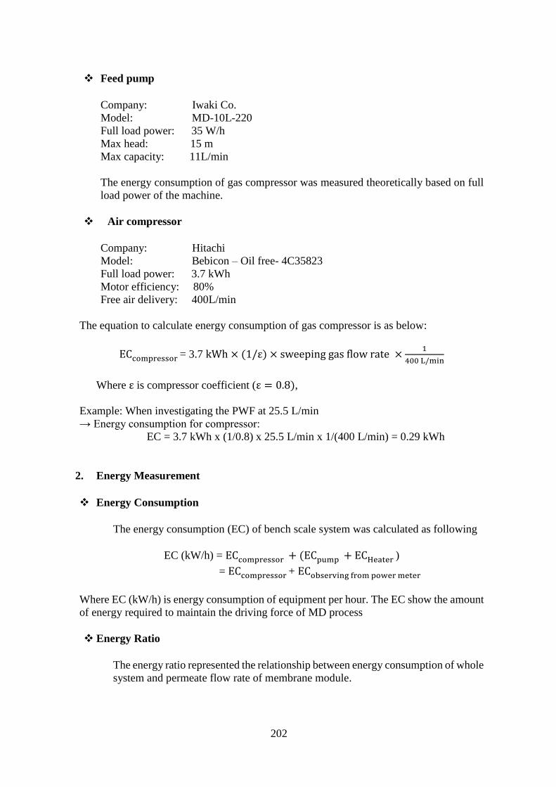
202
Feed pump
Company: Iwaki Co.
Model: MD-10L-220
Full load power: 35 W/h
Max head: 15 m
Max capacity: 11L/min
The energy consumption of gas compressor was measured theoretically based on full
load power of the machine.
Air compressor
Company: Hitachi
Model: Bebicon – Oil free- 4C35823
Full load power: 3.7 kWh
Motor efficiency: 80%
Free air delivery: 400L/min
The equation to calculate energy consumption of gas compressor is as below:
ECcompressor = 3.7 kWh × (1/ε) × sweeping gas flow rate ×1
400 L/min
Where ε is compressor coefficient (ε = 0.8),
Example: When investigating the PWF at 25.5 L/min
→ Energy consumption for compressor:
EC = 3.7 kWh x (1/0.8) x 25.5 L/min x 1/(400 L/min) = 0.29 kWh
2. Energy Measurement
Energy Consumption
The energy consumption (EC) of bench scale system was calculated as following
EC (kW/h) = ECcompressor + (ECpump + ECHeater )
= ECcompressor + ECobserving from power meter
Where EC (kW/h) is energy consumption of equipment per hour. The EC show the amount
of energy required to maintain the driving force of MD process
Energy Ratio
The energy ratio represented the relationship between energy consumption of whole
system and permeate flow rate of membrane module.
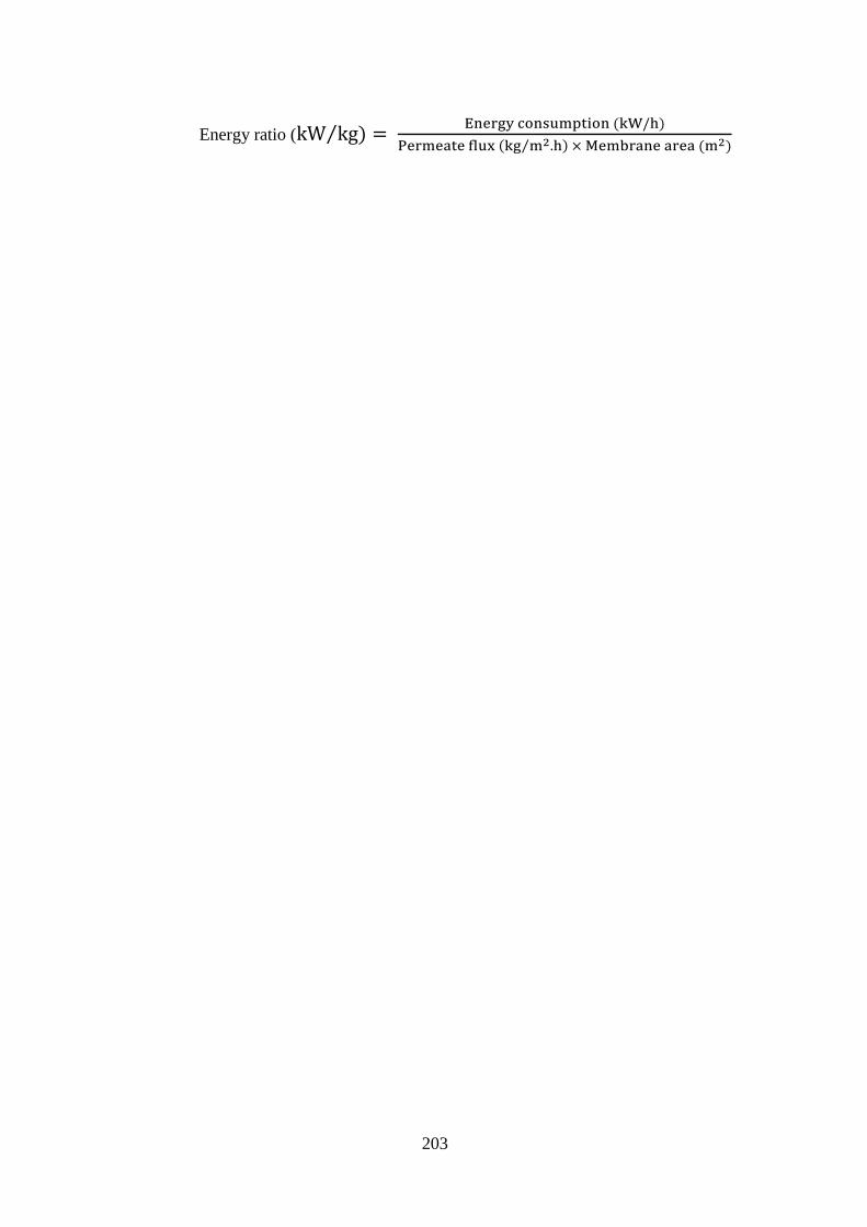
203
Energy ratio (kW kg)⁄ = Energy consumption (kW/h)
Permeate flux (kg m2⁄ .h) × Membrane area (m2)