optimizing feedforward artificial neural network architecture

ARTICLE IN PRESS

0952-1976/$ - se

doi:10.1016/j.en

�CorrespondE-mail addr

Engineering Applications of Artificial Intelligence 20 (2007) 365–382

www.elsevier.com/locate/engappai

Optimizing feedforward artificial neural network architecture

P.G. Benardos, G.-C. Vosniakos�

School of Mechanical Engineering, Manufacturing Technology Division, National Technical University of Athens, Heroon Polytehneiou 9,

157 80 Zografou, Athens, Greece

Received 7 December 2004; received in revised form 7 April 2006; accepted 29 June 2006

Available online 12 September 2006

Abstract

Despite the fact that feedforward artificial neural networks (ANNs) have been a hot topic of research for many years there still are

certain issues regarding the development of an ANN model, resulting in a lack of absolute guarantee that the model will perform well for

the problem at hand. The multitude of different approaches that have been adopted in order to deal with this problem have investigated

all aspects of the ANN modelling procedure, from training data collection and pre/post-processing to elaborate training schemes and

algorithms. Increased attention is especially directed to proposing a systematic way to establish an appropriate architecture in contrast to

the current common practice that calls for a repetitive trial-and-error process, which is time-consuming and produces uncertain results.

This paper proposes such a methodology for determining the best architecture and is based on the use of a genetic algorithm (GA) and

the development of novel criteria that quantify an ANN’s performance (both training and generalization) as well as its complexity. This

approach is implemented in software and tested based on experimental data capturing workpiece elastic deflection in turning. The

intention is to present simultaneously the approach’s theoretical background and its practical application in real-life engineering

problems. Results show that the approach performs better than a human expert, at the same time offering many advantages in

comparison to similar approaches found in literature.

r 2006 Elsevier Ltd. All rights reserved.

Keywords: Feedforward artificial neural networks; ANN architecture; Generalization; Genetic algorithms; Engineering problems

1. Introduction

Feedforward artificial neural networks (ANNs) arecurrently being used in a variety of applications with greatsuccess. Their first main advantage is that they do notrequire a user-specified problem solving algorithm (as is thecase with classic programming) but instead they ‘‘learn’’from examples, much like human beings. Their secondmain advantage is that they possess an inherent general-ization ability. This means that they can identify andrespond to patterns that are similar but not identical to theones with which they have been trained. On the other hand,the development of a feed-forward ANN model also posescertain problems, the most important being that there is noprior guarantee that the model will perform well for theproblem at hand. The whole ANN modelling procedurehas been investigated with the aim of introducing

e front matter r 2006 Elsevier Ltd. All rights reserved.

gappai.2006.06.005

ing author. Tel.: +30210 772 1457.

ess: [email protected] (G.-C. Vosniakos).

systematic ways that would lead to ANN models withconsistently good performance. The focus of these methodshas been in virtually every aspect of ANN modeldevelopment such as training data collection, data pre-and post-processing, different types of activation functions,initialization of weights, training algorithms and errorfunctions.While all of these affect ANN performance, increased

attention has been especially directed to finding the bestarchitecture. This is justified not only by the fact that it isdirectly associated with the model’s performance but alsobecause there is no theoretical background as to how thisarchitecture will be found or what it should look like. Themost typical method followed is a repetitive trial-and-errorprocess, during which, a large number of differentarchitectures is examined and compared to one another.Therefore, this process is very time-consuming and ismainly based on the human expert’s past experience andintuition, thus involving a high degree of uncertainty.Despite the increased level of research activity, the

www.elsevier.com/locate/engappai

dx.doi.org/10.1016/j.engappai.2006.06.005

mailto:[email protected]

ARTICLE IN PRESSP.G. Benardos, G.-C. Vosniakos / Engineering Applications of Artificial Intelligence 20 (2007) 365–382366

described problem has not yet been answered definitively.Nevertheless, the different approaches can be categorizedas follows: (i) empirical or statistical methods that are usedto study the effect of an ANN’s internal parameters andchoose appropriate values for them based on the model’sperformance (Khaw et al., 1995; Maier and Dandy,1998a, b; Benardos and Vosniakos, 2002). The mostsystematic and general of these methods utilizes theprinciples from Taguchi’s design of experiments (Ross,1996). The best combination of number of hidden layers,number of hidden neurons, choice of input factors, trainingalgorithm parameters etc. can be identified with thesemethods even though they are mostly case-oriented. (ii)hybrid methods such as fuzzy inference (Leski andCzogala, 1999) where the ANN can be interpreted as anadaptive fuzzy system or it can operate on fuzzy instead ofreal numbers. (iii) constructive and/or pruning algorithmsthat, respectively, add and/or remove neurons from aninitial architecture using a previously specified criterion toindicate how ANN performance is affected by the changes(Fahlman and Lebiere, 1990; Rathbun et al., 1997; Balkinand Ord, 2000; Islam and Murase, 2001; Jiang and Wah,2003; Ma and Khorasani, 2003). The basic rules are thatneurons are added when training is slow or when the meansquared error is larger than a specified value, and thatneurons are removed when a change in a neuron’s valuedoes not correspond to a change in the network’s responseor when the weight values that are associated with thisneuron remain constant for a large number of trainingepochs. Since both constructive and pruning algorithms arebasically gradient descent methods, their convergence tothe global minimum is not guaranteed and so they canbe trapped to a local minimum close to the point of thesearch space from which the algorithm started. (iv)evolutionary strategies that search over topology spaceby varying the number of hidden layers and hiddenneurons through application of genetic operators andevaluation of the different architectures according to anobjective function (Bebis et al., 1997; Liu and Yao, 1997;Yao and Liu, 1997, 1998; Castillo et al., 2000; Arifovic andGencay, 2001).

This paper proposes a methodology for determining thebest architecture that falls into this last category. It is basedon the use of a genetic algorithm (GA) and the develop-ment of novel criteria that quantify an ANN’s perfor-mance (both training and generalization) as well as itscomplexity. The detailed presentation of the approach isgiven in Section 2 of the paper, and a critique of its maindifferences and advantages in comparison to similarmethods is presented there, too, in order to highlight itsoriginality.

2. The approach

In order to understand the problem it is necessary toclosely examine the characteristics of a feedforward ANN.

There are four elements that comprise the ANN’sarchitecture:

1.
The number of layers. 2. The number of neurons in each layer. 3. The activation function of each layer. 4. The training algorithm (because this determines the final
value of the weights and biases).

Regarding the number of layers, the only certainty is thatthere should be an input and an output layer so as to beable to present and obtain data to and from the ANN,respectively. The number of neurons in each of these twolayers is specified by the number of input and outputparameters that are used to model each problem so it isreadily determined. Therefore, the objective is to find thenumber of hidden layers and the number of neurons ineach hidden layer. Unfortunately, it is not possible totheoretically determine how many hidden layers or neuronsare needed for each problem.The activation functions are chosen based on the kind of

data that are available (binary, bipolar, decimal, etc.) andthe type of layer. For instance, the identity function isalmost always used in the input layer, while continuousnon-linear sigmoid functions are used in the hidden layers(usually the hyperbolic tangent function).The training algorithm influences to a far greater extent

the training speed, performance of an ANN (training error)or the necessary computing power rather than thearchitecture itself.Summarizing, it is safe to assume that the most critical

elements of a feedforward ANN architecture are thenumber of hidden layers and hidden neurons. These arealso the elements that largely affect the generalizationability of the ANN model as a too complex model mayoverfit the training data and thus exhibit poor general-ization while a not complex enough model may beinsufficient to approximate the potential non-linear corre-lations in the training data.The approach presented in this paper considers the

problem as one of multi-objective optimization. Thesolution space consists of all the different combinationsof hidden layers and hidden neurons, i.e. of all thearchitectures. Given the complex nature of the problem,a GA is employed to search the solution space for the‘‘best’’ architectures, where ‘‘best’’ is defined according to aset of predefined criteria. The basic idea behind the GAs isthat the optimal solution will be found in areas of thesolution space that contain good solutions and that theseareas can be identified through robust sampling. Practi-cally, this means that the solution space is divided intosubsets that are evaluated in order to find the best solution.The sampling process is performed repetitively, whilemaintaining the best solutions from each subset until theoptimum solution is found. The mathematical analogue ofthis process dictates the coding of the solutions in binarystrings called chromosomes, the use of an objective

ARTICLE IN PRESSP.G. Benardos, G.-C. Vosniakos / Engineering Applications of Artificial Intelligence 20 (2007) 365–382 367

function to evaluate how ‘‘good’’ a chromosome is andcertain operators that are responsible for the samplingprocedure.

The three main reasons for the adoption of a GA insteadof a conventional optimization algorithm in this approachare listed below:

�
The GA operates on a coded form of the problem’sparameters rather than on the parameters themselves.This results in the search of the global minimum beingindependent from the continuity of the function or theexistence of its derivative. � The sampling procedure does not start from a single
point of the solution space but from a set of points(initial population), therefore the possibility of entrap-ment in a local minimum is reduced.
� The sampling procedure is carried out using the genetic
operators which are stochastic and not deterministic innature.

The developed methodology consists of the followingsteps:

1.
A random initial population is formed using an indirectencoding scheme, where only the number of hiddenlayers and number of neurons in each hidden layer isencoded in the chromosome.
2.
The initial population is decoded to its phenotypic formand the various ANN architectures are created.
3.
Each of these models has its weights initialized using theNguyen–Widrow method and is subsequently trainedwith the Levenberg–Marquardt algorithm along withearly stopping. For this purpose, the available data mustbe divided into three subsets, namely the training,validation and testing subset. The first is used to trainthe ANN and the second dictates that when the errorremains constant for a predefined number of epochs orstarts to increase rapidly training should stop becausethe ANN has started to overfit the data. The testingsubset (unknown data to the ANN) is used aftercompletion of the training to assess the generalizationperformance of the ANN model.
4.
For each trained ANN architecture the values of thecriteria that quantify its performance (both training andgeneralization) as well as its complexity are calculated.
5.
Based on these values the entire population is evaluated,i.e. the objective function value for each ANN is calcu-lated and the one with the lower objective value is stored.
6.
The evolutionary process begins by applying the geneticoperators (fitness, selection, crossover and mutation) tothe coded population and new offspring are produced.
7.
Steps 2–5 are executed again, this time for the offspringthat are produced.
8.
The offspring are reinserted into the population repla-cing the least fit parents. The best initial ANN model,which was previously stored, is compared to the bestoffspring ANN model and the better one is stored.
9.
Steps 6–8 are executed until the GA converges or themaximum number of generations is reached.
A flowchart of the described approach is presented inFig. 1.Compared to other similar approaches that involve

evolutionary algorithms, the proposed methodology ex-hibits three major differences/advantages. Firstly, it isargued in Yao and Liu (1997) that using a phenotype’sfitness to represent the genotype’s (the term was usedsynonymously to the objective function value) fitnessintroduces noise that can mislead the evolution. Theproposed methodology deals with this issue in twoways: (i) by employing an indirect encoding scheme, whichguarantees that for each phenotype there is only onegenotype and vice-versa and (ii) by randomly initializingeach architecture’s weights prior to training. Point(i) ensures that the relationship between two phenotypes’fitnesses is always valid for their genotypic representationsand point (ii) that the fitness of any one architecture didnot depend on a favourable initialization of weightsbut rather it was due to the architecture itself resulting inmore robust architecture performance. Secondly, in orderto reduce computation time and at the same time avoidoverfitting of the training data, a partial training schemeis adopted in Bebis et al. (1997). An ANN could befurther trained if all other attempts to reduce its errorfailed. This could lead to slow convergence of theevolutionary process (in the best case) and strangebehaviour of the GA (in the worst case) because eachANN’s performance could very easily be dependent onunfavourable initializations or unsuitable training algo-rithms. If the ANN is not given ‘‘enough’’ time to learn, itis not right to conclude that a chosen architecture cannotperform well. Therefore, early stopping was used in theproposed approach. This choice was made because earlystopping can allow for a small network (which is fast totrain) to be trained for a sufficient number of epochs inorder to learn the data associations and at the same timeprevent a very complex network (which is slow to train)from overfitting the data. In this context, early stoppingacts as a kind of ‘‘filter’’ that adjusts training speed andgeneralization performance simultaneously. Thirdly, andmost importantly, all of the referenced papers (Bebis et al.,1997; Liu and Yao, 1997; Yao and Liu, 1997, 1998; Castilloet al., 2000; Arifovic and Gencay, 2001) claim that eachevolved architecture’s generalization performance is eval-uated, but in reality this is not entirely true. Either avalidation set is used during the evolutionary process toestimate the generalization ability of an ANN or pruningtechniques are employed to maintain a relatively smallsized ANN. While both of these measures favour thegeneralization ability of the network, they can neitherguarantee nor quantify this ability for the final evolvedarchitecture. In contrast, two of the four criteria that formthe objective function in the present approach are directmeasures of the generalization error (calculated after each

ARTICLE IN PRESS

Fig. 1. Philosophy of the GA for the developed methodology.

P.G. Benardos, G.-C. Vosniakos / Engineering Applications of Artificial Intelligence 20 (2007) 365–382368

training is completed by using the testing set) during theactual evolution.

3. Methodology development

3.1. Chromosome coding

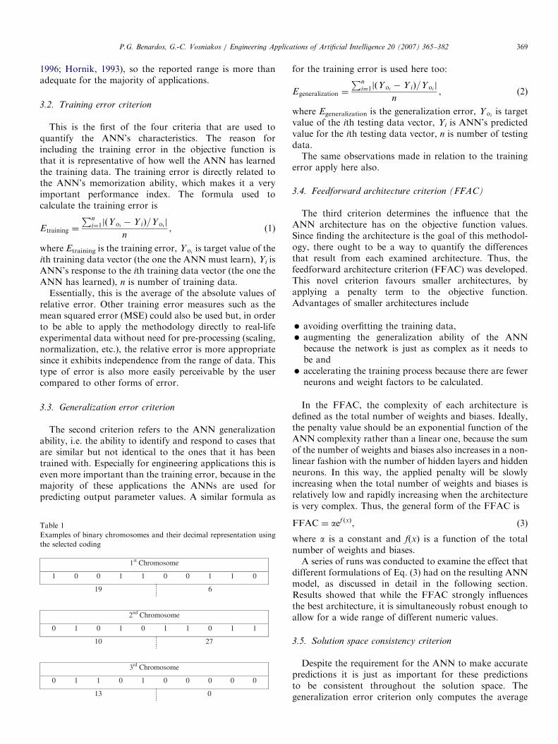
An indirect encoding scheme was selected, i.e. onlyinformation about the number of hidden layers andnumber of hidden neurons in each layer is contained inthe chromosomes. The problem’s parameters were coded ina 10-bit binary chromosome. The first and second group of5 bits correspond to the number of neurons in the first andsecond hidden layer, respectively. Due to the binary codingand the number of bits used, the number of neurons in eachhidden layer is found in the interval [0,31] since

24+23+22+21+20 ¼ 31. In this way, the chromosomecontains information for both the number of hidden layersand the number of neurons in each layer. To furtherexplain the applied coding three different chromosomes,along with their decoded form, are given in Table 1.It is obvious that by increasing the chromosome length,

i.e. the number of available bits, any feedforwardarchitecture can be created, so this encoding schemeensures the generality of the methodology. The limits,namely up to 2 hidden layers and 31 neurons in eachhidden layer, are imposed for practical reasons only(computation time). In any case, it has been shown thatfor feedforward ANNs with continuous non-linear hiddenlayer activation functions, one hidden layer with anarbitrarily large number of neurons suffices for the‘‘universal approximation’’ property (Bishop, 1995; Ripley,


1996; Hornik, 1993), so the reported range is more thanadequate for the majority of applications.

3.2. Training error criterion

This is the first of the four criteria that are used toquantify the ANN’s characteristics. The reason forincluding the training error in the objective function isthat it is representative of how well the ANN has learnedthe training data. The training error is directly related tothe ANN’s memorization ability, which makes it a veryimportant performance index. The formula used tocalculate the training error is

Etraining ¼

Pni¼1jðY oi

� Y iÞ=Yoij

n, (1)

where Etraining is the training error, Y oiis target value of the

ith training data vector (the one the ANN must learn), Yi isANN’s response to the ith training data vector (the one theANN has learned), n is number of training data.

Essentially, this is the average of the absolute values ofrelative error. Other training error measures such as themean squared error (MSE) could also be used but, in orderto be able to apply the methodology directly to real-lifeexperimental data without need for pre-processing (scaling,normalization, etc.), the relative error is more appropriatesince it exhibits independence from the range of data. Thistype of error is also more easily perceivable by the usercompared to other forms of error.

3.3. Generalization error criterion

The second criterion refers to the ANN generalizationability, i.e. the ability to identify and respond to cases thatare similar but not identical to the ones that it has beentrained with. Especially for engineering applications this iseven more important than the training error, because in themajority of these applications the ANNs are used forpredicting output parameter values. A similar formula as

Table 1

Examples of binary chromosomes and their decimal representation using

the selected coding

1st Chromosome

1 0 0 1 1 0 0 1 1 0

19 6

2nd Chromosome

0 1 0 1 0 1 1 0 1 1

10 27

3rd Chromosome

0 1 1 0 1 0 0 0 0 0

13 0

for the training error is used here too:

Egeneralization ¼

Pni¼1jðYoi

� Y iÞ=Yoij

n, (2)

where Egeneralization is the generalization error, Yoiis target

value of the ith testing data vector, Yi is ANN’s predictedvalue for the ith testing data vector, n is number of testingdata.The same observations made in relation to the training

error apply here also.

3.4. Feedforward architecture criterion (FFAC)

The third criterion determines the influence that theANN architecture has on the objective function values.Since finding the architecture is the goal of this methodol-ogy, there ought to be a way to quantify the differencesthat result from each examined architecture. Thus, thefeedforward architecture criterion (FFAC) was developed.This novel criterion favours smaller architectures, byapplying a penalty term to the objective function.Advantages of smaller architectures include

�
avoiding overfitting the training data, � augmenting the generalization ability of the ANN
because the network is just as complex as it needs tobe and
� accelerating the training process because there are fewer
neurons and weight factors to be calculated.

In the FFAC, the complexity of each architecture isdefined as the total number of weights and biases. Ideally,the penalty value should be an exponential function of theANN complexity rather than a linear one, because the sumof the number of weights and biases also increases in a non-linear fashion with the number of hidden layers and hiddenneurons. In this way, the applied penalty will be slowlyincreasing when the total number of weights and biases isrelatively low and rapidly increasing when the architectureis very complex. Thus, the general form of the FFAC is

FFAC ¼ aef ðxÞ, (3)

where a is a constant and f(x) is a function of the totalnumber of weights and biases.A series of runs was conducted to examine the effect that

different formulations of Eq. (3) had on the resulting ANNmodel, as discussed in detail in the following section.Results showed that while the FFAC strongly influencesthe best architecture, it is simultaneously robust enough toallow for a wide range of different numeric values.

3.5. Solution space consistency criterion

Despite the requirement for the ANN to make accuratepredictions it is just as important for these predictionsto be consistent throughout the solution space. Thegeneralization error criterion only computes the average

ARTICLE IN PRESS

Table 2

Actions to be performed for the execution of the application

Read data from an Excel worksheet The user must specify the path of the Excel file containing the experimental data that are

automatically read by the application

Create the training, validation and testing data sets The user must enter the row ranges that each data set occupies in the Excel file

Set the GA parameters These include the population size, number of generations, the offspring size and the genetic operators

(selection, crossover and mutation)

Define the encoding scheme parameters These include the number of hidden layers and number of bits for each hidden layer

Set the input and output layer of the ANN The user must enter the number of input and output neurons

Customize the criteria penalties The customizable penalties are the FFAC and solution space consistency criterion

Run the GA.

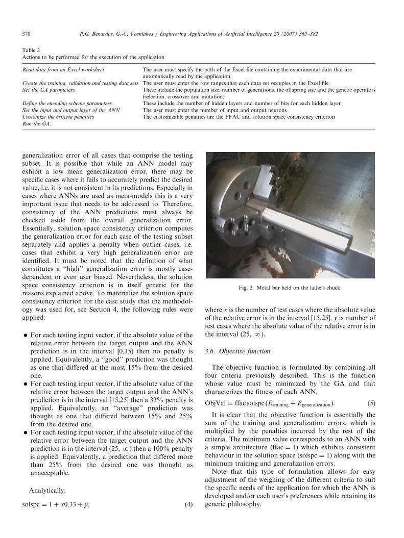
Fig. 2. Metal bar held on the lathe’s chuck.


generalization error of all cases that comprise the testingsubset. It is possible that while an ANN model mayexhibit a low mean generalization error, there may bespecific cases where it fails to accurately predict the desiredvalue, i.e. it is not consistent in its predictions. Especially incases where ANNs are used as meta-models this is a veryimportant issue that needs to be addressed to. Therefore,consistency of the ANN predictions must always bechecked aside from the overall generalization error.Essentially, solution space consistency criterion computesthe generalization error for each case of the testing subsetseparately and applies a penalty when outlier cases, i.e.cases that exhibit a very high generalization error areidentified. It must be noted that the definition of whatconstitutes a ‘‘high’’ generalization error is mostly case-dependent or even user biased. Nevertheless, the solutionspace consistency criterion is in itself generic for thereasons explained above. To materialize the solution spaceconsistency criterion for the case study that the methodol-ogy was used for, see Section 4, the following rules wereapplied:

�
For each testing input vector, if the absolute value of therelative error between the target output and the ANNprediction is in the interval [0,15) then no penalty isapplied. Equivalently, a ‘‘good’’ prediction was thoughtas one that differed at the most 15% from the desiredone. � For each testing input vector, if the absolute value of the
relative error between the target output and the ANN’sprediction is in the interval [15,25] then a 33% penalty isapplied. Equivalently, an ‘‘average’’ prediction wasthought as one that differed between 15% and 25%from the desired one.
� For each testing input vector, if the absolute value of the
relative error between the target output and the ANNprediction is in the interval (25, N) then a 100% penaltyis applied. Equivalently, a prediction that differed morethan 25% from the desired one was thought asunacceptable.

Analytically:

solspc ¼ 1þ x0:33þ y, (4)

where x is the number of test cases where the absolute valueof the relative error is in the interval [15,25], y is number oftest cases where the absolute value of the relative error is inthe interval (25, N).

3.6. Objective function

The objective function is formulated by combining allfour criteria previously described. This is the functionwhose value must be minimized by the GA and thatcharacterizes the fitness of each ANN.

ObjVal ¼ ffac solspc ðEtraining þ EgeneralizationÞ. (5)

It is clear that the objective function is essentially thesum of the training and generalization errors, which ismultiplied by the penalties incurred by the rest of thecriteria. The minimum value corresponds to an ANN witha simple architecture (ffac ¼ 1) which exhibits consistentbehaviour in the solution space (solspc ¼ 1) along with theminimum training and generalization errors.Note that this type of formulation allows for easy

adjustment of the weighing of the different criteria to suitthe specific needs of the application for which the ANN isdeveloped and/or each user’s preferences while retaining itsgeneric philosophy.


3.7. Software implementation

The described methodology was implemented in theMATLAB programming environment. The philosophy of

321

3

1

2

50 200

150100

7020

120°

120°

Fig. 3. Diameter measurement positions along the workpiece.

Table 3

Experimental data for the development of the ANN model

a/a Depth of

cut (mm)

(radius)

Feed

(mm/rev)

RPM L/D Li/L (mm)

1 0.175 0.150 1080 3.8706 0.500 �0.0042

2 0.175 0.150 1080 3.8706 0.650 �0.0065

3 0.175 0.150 1080 3.8706 0.900 �0.0035

4 0.350 0.150 800 3.9233 0.250 �0.0018

5 0.350 0.150 800 3.9233 0.900 �0.0058

6 0.350 0.200 925 3.9765 0.250 �0.0063

7 0.350 0.200 925 3.9765 0.500 �0.0093

8 0.350 0.200 925 3.9765 0.650 �0.0105

9 0.350 0.250 985 4.0312 0.500 �0.0093

10 0.350 0.250 985 4.0312 0.650 �0.0073

11 0.350 0.250 985 4.0312 0.900 �0.0138

12 0.500 0.150 985 4.1183 0.250 0.0222

13 0.500 0.150 985 4.1183 0.900 0.0308

14 0.500 0.200 860 4.2035 0.250 �0.0065

15 0.500 0.200 860 4.2035 0.500 �0.0065

16 0.500 0.200 860 4.2035 0.650 �0.0083

17 0.500 0.250 910 4.2903 0.500 �0.0170

18 0.500 0.250 910 4.2903 0.650 �0.0188

19 0.500 0.250 910 4.2903 0.900 �0.0263

20 0.600 0.100 1020 4.4098 0.250 0.0242

21 0.600 0.100 1020 4.4098 0.900 0.0447

22 0.600 0.150 1150 4.5283 0.250 �0.0045

23 0.600 0.150 1150 4.5283 0.500 �0.0047

24 0.600 0.150 1150 4.5283 0.650 �0.0060

25 0.600 0.200 1300 4.6526 0.250 �0.0077

26 0.600 0.200 1300 4.6526 0.500 �0.0102

27 0.600 0.200 1300 4.6526 0.650 �0.0108

28 0.600 0.200 1300 4.6526 0.900 �0.0130

29 0.175 0.150 1080 3.8706 0.250 �0.0088

30 0.350 0.150 800 3.9233 0.650 �0.0022

31 0.350 0.250 985 4.0312 0.250 �0.0075

32 0.500 0.150 985 4.1183 0.650 0.0240

33 0.500 0.250 910 4.2903 0.250 �0.0135

34 0.600 0.100 1020 4.4098 0.650 0.0308

35 0.350 0.150 800 3.9233 0.500 �0.0030

36 0.350 0.200 925 3.9765 0.900 �0.0103

37 0.500 0.150 985 4.1183 0.500 0.0233

38 0.500 0.200 860 4.2035 0.900 �0.0102

39 0.600 0.100 1020 4.4098 0.500 0.0273

40 0.600 0.150 1150 4.5283 0.900 �0.0110

the implementation is very simple and is summarized inTable 2.The goal was to develop an application that could be

efficiently used by someone with little to no experience inthe fields of ANNs and GAs, while maintaining thegenerality of the methodology. Therefore, any requiredinformation has been categorized in variables that must bedefined only once before running the application. When theapplication terminates the best ANN model can be directlyaccessed from the MATLAB workspace.

4. Case study: elastic deflection in turning results

The methodology was tested using experimental dataoriginating from a turning process on a Victor VTPlus-20CNC lathe equipped with a FANUC Series O-T controller.A steel bar (C45) clamped on one end (Fig. 2) was reducedin diameter with a variety of cutting conditions.The object was to examine the influence of these

parameters along with the L/D ratio (L and D being thebar’s overhang length and diameter before the cut,respectively) and the elastic deflection of the bar due tothe cutting forces on the dimensional deviations of the finalpart. These were quantified as the differences between thedesired and actual depth of cut. For this purpose, aftereach cut, a series of diameter measurements was conductedin different positions along the bar (Fig. 3) using calibratedelectronic precision micrometers. These measurementswere compared with the programmed depth of cut tocalculate the dimensional deviations. The experimentaldata were used to develop an ANN model that would beable to predict the deviations of the turned workpiece priorto the cut.Subsequently, the architecture obtained by the proposed

methodology was to be compared with the one that anexperienced researcher would come up with for the sameproblem by following common practice of trial-and-error.In the latter case, the best performing architecture was

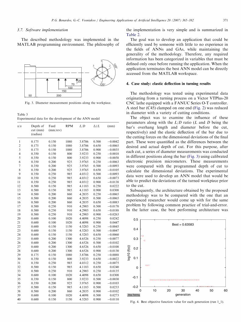
0.5

0.4

0.3

0.2

0.1

0

-0.1

-0.20 10 20 30 40 50 60

generation

log1

0 (f

(x))

Best = 0.63583

Stop Training

Fig. 4. Best objective function value for each generation (run 1_1).

ARTICLE IN PRESS

0.06

0.04

0.02

0

-0.02

-0.040 5 10 15 20 25 30

0.5

0

-0.50 5 10 15 20 25 30

0.03

0.02

0.01

0

-0.01

-0.021 1.5 2 2.5 3 3.5 4 4.5 5 5.5 6

0.2

0.3

0.1

-0.2

-0.1

0

1 2 3 4 5 6

(a)

(b)

Fig. 5. (a) Relative error for each case of the training subset (run 1_1). (b) Relative error for each case of the testing subset (run 1_1).


5� 3� 1, i.e. with one hidden layer and three neurons,resulting in a total of 22 weights and biases. The meangeneralization error of this model was equal to 11.99%.

The complete data set is shown in Table 3. The trainingsubset consists of data vectors 1–28 (70% of the total data),the validation subset of data vectors 29–34 (15% of thetotal data), while the testing subset of data vectors 35–40(15% of the total data).

According to Table 2, the next step was to set the GAparameters. Population size was selected to be constant at25 chromosomes, while the GA was executed for 50generations and the number of offspring in each generationwas set to 92% of the population size (23 new individualsare created).

For the genetic operator selection, the stochasticuniversal sampling (SUS) method was used (MathWorks).Instead of the single selection pointer employed in roulettewheel methods, SUS uses N equally spaced pointers, whereN is the number of selections required. The population isshuffled randomly and a single random number in therange [0 Sum/N] is generated, ptr. The N individuals arethen chosen by generating the N pointers spaced by 1, [ptr,ptr+1, y, ptr+N�1], and selecting the individuals whosefitnesses span the positions of the pointers.Single-point crossover was used to produce the off-

spring. In this method, an integer position number in therange [1, L�1], where L is the chromosome length,is selected uniformly at random and the two parent

ARTICLE IN PRESS

Table 5

Detailed results of the five runs (second case)

Run no Final_ANN

architecture

Total number of

weights and

biases

Mean absolute

generalization

error

2_1 5� 14� 1� 1 101 0.1415

2_2 5� 14� 1� 1 101 0.1896

2_3 5� 4� 8� 1 73 0.2266

2_4 5� 14� 1 99 0.1117

2_5 5� 2� 18� 1 85 0.1580

Mean 91.8 0.1655

Std 12.5 0.0443

Var 155.2 0.0020

0.6

0.5

0.4

Best = 0.47591

P.G. Benardos, G.-C. Vosniakos / Engineering Applications of Artificial Intelligence 20 (2007) 365–382 373

chromosomes exchange their strings about this position.The crossover operator is not applied on all chromosomesof the population but with a set probability according towhich the chromosome pair is selected. The probabilityused was 70%.

Finally, a mutation probability of 5% was chosen. In thecase of binary coded chromosomes mutation changes thevalue of a bit in the chromosome from 0 to 1 or vice versa,according to the given probability. Mutation ensures thatfor any given coding all strings have a chance to beevaluated and that, if a good chromosome is lost throughselection and crossover, it will reappear in future genera-tions.

In total, a series of six different cases were evaluated.Five of them involved different formulations of the FFACin order to determine the robustness of the criterion. Thegoal was to investigate how the ANNs’ characteristics areinfluenced by the different setting of the criterion. Anadditional case in which the FFAC and the solution spaceconsistency criteria were not included in the objectivefunction was also investigated in order to test theirinfluence to the final ANN model’s performance. For eachcase, five different runs of the GA were executed so as toreduce uncertainty of performance due to the stochasticnature of the GAs. After each run, the history of the bestobjective value in each generation was recorded and theANN model with the overall lowest objective functionvalue was stored. The number of weights and biases as wellas the training and generalization performances of thismodel were calculated and presented graphically. Further-more, after completion of each case (five runs) the meanand standard deviation values for the sum of weights andbiases and for the generalization error of the best five ANNmodels were also calculated. These were subsequently usedto conduct t-tests to determine if there are statisticallysignificant differences between the cases. All the results arepresented below.

4.1. First case

The following equation was used for the FFAC:

FFAC ¼ e0:001x. (6)

Table 4

Detailed results of the five runs (first case)

Run no Final_ANN

architecture

Total number of

weights and

biases

Mean absolute

generalization

error

1_1 5� 10� 3� 1 97 0.0918

1_2 5� 8� 4� 1 89 0.1969

1_3 5� 10� 3� 1 97 0.1453

1_4 5� 12� 4� 1 129 0.1482

1_5 5� 3� 10� 1 69 0.1533

Mean 96.2 0.1471

Std 21.6 0.0374

Var 467.2 0.0014

This formulation effectively penalizes architectures withmore than 500 total weights and biases so it provides a lotof room for complex networks. The results for all five runsare presented in Table 4. The history of the best objectivefunction value as well as the training and generalizationperformance of the overall best ANN model, correspond-ing to run number 1_1, are displayed in Figs. 4, 5a and brespectively.Figs. 5a and b each contain two charts, the top one

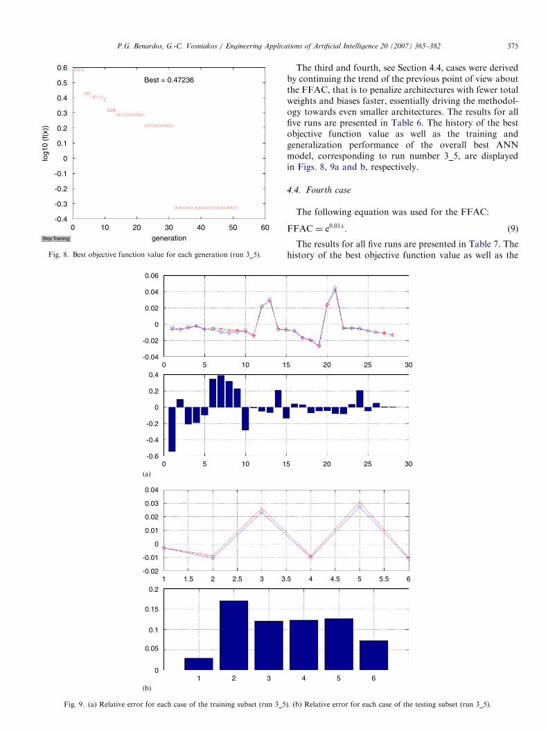
displaying the desired value for each case (denoted bycircles) and the ANN’s response (denoted by crosses) andthe bottom one displaying the calculated relative errorbetween the two as a bar graph. In both sub-graphs thehorizontal axis represents the case’s number and thevertical one the difference between the desired and actualdepth of cut as described in the case study.

4.2. Second case


FFAC ¼ e0:002x (7)

0 10 20 30 40 50 60generation

log1

0 (f

(x))

Stop Training

0.3

0.2

0.1

0

-0.1

-0.2

-0.3

-0.4


ARTICLE IN PRESS

0.06

0.04

0.02

0

-0.02

-0.040 5 10 15 20 25 30

0.4

0.2

-0.2

0

-0.40 5 10 15 20 25 30

0.04

0.03

0.02

0.01

0

-0.01

-0.021 1.5 2 2.5 3 3.5 4 4.5 5 5.5 6

0.2

0.3

0.1

-0.1

0

1 2 3 4 5 6

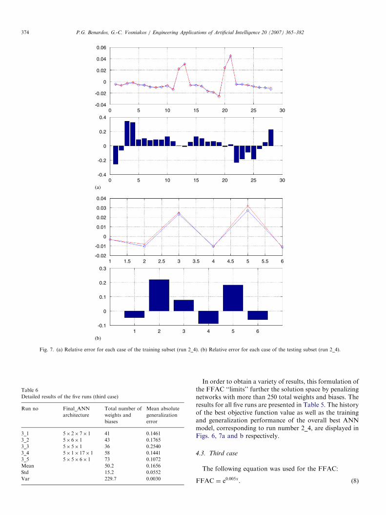
(a)

(b)


Table 6

Detailed results of the five runs (third case)

Run no Final_ANN

architecture

Total number of

weights and

biases

Mean absolute

generalization

error

3_1 5� 2� 7� 1 41 0.1461

3_2 5� 6� 1 43 0.1765

3_3 5� 5� 1 36 0.2540

3_4 5� 1� 17� 1 58 0.1441

3_5 5� 5� 6� 1 73 0.1072

Mean 50.2 0.1656

Std 15.2 0.0552

Var 229.7 0.0030


In order to obtain a variety of results, this formulation ofthe FFAC ‘‘limits’’ further the solution space by penalizingnetworks with more than 250 total weights and biases. Theresults for all five runs are presented in Table 5. The historyof the best objective function value as well as the trainingand generalization performance of the overall best ANNmodel, corresponding to run number 2_4, are displayed inFigs. 6, 7a and b respectively.

4.3. Third case


FFAC ¼ e0:005x. (8)

ARTICLE IN PRESS

0 10 20 30 40 50 60generation

log1

0 (f

(x))

Best = 0.47236

Stop Training

0.6

0.5

0.4

0.3

0.2

0.1

0

-0.1

-0.2

-0.3

-0.4


0.06

0.04

0.02

0

-0.02

-0.040 5 10 1

0.4

0.2

-0.2

0

-0.4

-0.60 5 10 1

0.04

0.03

0.02

0.01

0

-0.01

-0.021 1.5 2 2.5 3 3

0.15

0.2

0.1

0

0.05

1 2 3

(a)

(b)

Fig. 9. (a) Relative error for each case of the training subset (run 3_5


The third and fourth, see Section 4.4, cases were derivedby continuing the trend of the previous point of view aboutthe FFAC, that is to penalize architectures with fewer totalweights and biases faster, essentially driving the methodol-ogy towards even smaller architectures. The results for allfive runs are presented in Table 6. The history of the bestobjective function value as well as the training andgeneralization performance of the overall best ANNmodel, corresponding to run number 3_5, are displayedin Figs. 8, 9a and b, respectively.

4.4. Fourth case


FFAC ¼ e0:01x. (9)

The results for all five runs are presented in Table 7. Thehistory of the best objective function value as well as the

5 20 25 30

5 20 25 30

.5 4 4.5 5 5.5 6

4 5 6

). (b) Relative error for each case of the testing subset (run 3_5).

ARTICLE IN PRESS

Table 7

Detailed results of the five runs (fourth case)

Run no Final_ANN

architecture

Total number of

weights and

biases

Mean absolute

generalization

error

4_1 5� 3� 2� 1 29 0.1810

4_2 5� 3� 1� 1 24 0.1871

4_3 5� 2� 1� 1 17 0.1628

4_4 5� 3� 3� 1 34 0.1916

4_5 5� 4� 2� 1 37 0.0896

Mean 28.2 0.1624

Std 8.0 0.0422

Var 63.7 0.0018

1.2

0.8

0.4

0.2

0

-0.2

1

0.6

0 10 20 30 40 50 60generation

log1

0 (f

(x))

Best = 0.81089

Stop Training



training and generalization performance of the overall bestANN model, corresponding to run number 4_5, aredisplayed in Figs. 10, 11a and b respectively.

4.5. Fifth case


FFAC ¼ e0:00001x2

. (10)

The difference of this case to the previous four is that thetotal number of weights and biases in the exponent issquared. Thus, this formulation delays the penalization ofarchitectures but when it does penalizes the more complexones it does so in a very aggressive manner. In practice, thisallows the GA to more freely search a portion of thesolution space while simultaneously ‘‘limiting’’ its size asthe previous ones did. The results for all five runs arepresented in Table 8. The history of the best objectivefunction value as well as the training and generalizationperformance of the overall best ANN model, correspond-ing to run number 5_3, are displayed in Figs. 12, 13a and brespectively.

4.6. Sixth case

The sixth case was executed with the objective functioncontaining only the training and generalization errorcriteria (Eq. (11)).

ObjVal ¼ ðEtraining þ EgeneralizationÞ. (11)

The results for all five runs are presented in Table 9. Thehistory of the best objective function value as well as thetraining and generalization performance of the overall bestANN model, corresponding to run number 6_3, aredisplayed in Figs. 14, 15a and b respectively.

5. Analysing results

In order to analyse the obtained results a series ofhypothesis tests was conducted. The aim was to determinewhether statistically significant differences exist among thecases, i.e. whether the different criteria formulationsinfluence the results. For every possible pair of cases, atwo sample t-test (Snedecor and Cochran, 1989) wasconducted to compare the mean values of the total numberof weights and biases as well as the mean values of themean absolute generalization error. The two sample t-testis defined as

H0 : m1 ¼ m2,

Ha : m1am2,

t0 ¼x1 � x2ffiffiffiffiffiffiffiffiffiffiffiffiffiffiffiffiffiffiffiffiffiffiffiffiffiffiffiffiffiffiffiffiffiffiffiffiffi

ðs21=N1Þ þ ðs22=N2Þ

q , (12)

where H0 is the null hypothesis that the two populationmeans (m1 and m2, respectively) are equal, Ha is thealternative hypothesis that the two population means areunequal, t0 is the test statistic, x1 and x2 are the samplemeans, s1

2 and s22 are the sample variances and N1 and N2

are the sample sizes.By conducting the test at significance level a ¼ 0:05, the

null hypothesis is rejected if

jt0jXtð1� ða=2Þ; nÞ, (13)

where t is the critical value of the t distribution with ndegrees of freedom:

n ¼ððs21=N1Þ þ ðs

22=N2ÞÞ

2

ððs21=N1Þ2=ðN1 � 1ÞÞ þ ððs22=N2Þ

2=ðN2 � 1ÞÞ. (14)

In this way, if the null hypothesis is accepted it isconcluded that the means are statistically equal and if it isrejected it is concluded that there is a statistical differencebetween them.Since six cases were evaluated the possible number of

pairs is

6

2

� �¼

6!

2! � ð6� 2Þ!¼

6!

2! � 4!¼

5 � 6

1 � 2¼ 15.

ARTICLE IN PRESS

0.06

0.04

0.02

0

-0.02

-0.040 5 10 15 20 25 30

0.5

0

-0.5

-10 5 10 15 20 25 30

0.03

0.02

0.01

0

-0.01

-0.021 1.5 2 2.5 3 3.5 4 4.5 5 5.5 6

0.3

0.2

0.1

0

-0.11 2 3 4 5 6

(a)

(b)


Table 8

Detailed results of the five runs (fifth case)

Run no Final_ANN

architecture

Total number of

weights and

biases

Mean absolute

generalization

error

5_1 5� 4� 8� 1 73 0.1999

5_2 5� 5� 5� 1 66 0.1451

5_3 5� 9� 1 64 0.1080

5_4 5� 4� 4� 1 49 0.1848

5_5 5� 7� 2� 1 61 0.1896

Mean 62.6 0.1655

Std 8.8 0.0383

Var 77.3 0.0015


5.1. Total number of weights and biases

Using Eq. (12), the test statistic for all pairs can becalculated based on data of Tables 4–9. The results arepresented in Table 10.Subsequently, the degrees of freedom for every case pair

are also calculated through Eq. (14) (Table 11).It is then possible to determine the critical value of the t

distribution (Table 12).By applying the criterion for rejecting the null

hypothesis (Eq. (13)), the final decision of eacht-test is presented in Table 13. Please note that inthis table acceptance of the null hypothesis is denoted

ARTICLE IN PRESS

0.4

0.2

0

-0.1

-0.2

-0.3

-0.4

0.3

0.1

0 10 20 30 40 50 60generation

log1

0 (f

(x))

Best = 0.46233

Stop Training


0.06

0.04

0.02

0

-0.02

-0.040 5 10 1

0.4

0.2

0

-0.2

-0.40 5 10 1

0.04

0.03

0.02

0.01

0

-0.01

-0.021 1.5 2 2.5 3 3

0.4

0.3

0.2

0.1

0

-0.11 2 3

(a)

(b)

Fig. 13. (a) Relative error for each case of the training subset (run 5_


by 1 and rejection of the null hypothesis is denotedby 0.

5.2. Mean absolute generalization error

Using Eq. (12), the test statistic for all pairs can becalculated based on data of Tables 4–9. The results arepresented in Table 14.Subsequently, the degrees of freedom for every case pair

are also calculated through Eq. (14) (Table 15).It is then possible to determine the critical value of the t

distribution (Table 16).By applying the criterion for rejecting the null hypothesis

(Eq. (13)), the final decision of each t-test is presented inTable 17. Please note that in this table acceptance of thenull hypothesis is denoted by 1 and rejection of the nullhypothesis is denoted by 0.

5 20 25 30

5 20 25 30

.5 4 4.5 5 5.5 6

4 5 6

3). (b) Relative error for each case of the testing subset (run 5_3).

ARTICLE IN PRESS

Table 9

Detailed results of the five runs (sixth case)

Run no Final_ANN

architecture

Total number of

weights and

biases

Mean absolute

generalization

error

6_1 5� 15� 1 106 0.3031

6_2 5� 8� 8� 1 129 0.2158

6_3 5� 2� 29� 1 129 0.2059

6_4 5� 16� 1 113 0.2568

6_5 5� 17� 2� 1 141 0.2217

Mean 123.6 0.2407

Std 14.0 0.0398

Var 195.8 0.0016

0.2

0.1

0

-0.1

-0.2

-0.3

-0.4

-0.5

-0.60 10 20 30 40 50 60

generation

log1

0 (f

(x))

Best = 0.27725

Stop Training



6. Discussion

Separating the sixth case, for the moment, and concen-trating on the other five the conclusion is that there is aconsiderable variation in terms of the complexity of theANN models that are created. With the exception of twocase pairs out of ten, namely 1–2 and 3–5, differentformulations of the FFAC resulted in statistically sig-nificant differences in the size of the networks. Specifically,the less complex network contained only 17 weights andbiases (run 4_3) and the most complex one contained 129(run 1_4). This shows that the FFAC actually influencesthe GA and that the larger the applied penalty is, thesmaller (containing less total weights and biases) theevolved ANN architectures get. The fact that two casepairs are statistically equal can be easily explained by thefact that the differences in the penalties that are applied bythe FFAC formulations corresponding to these pairs arealso small.

At the same time, there does not seem to be anystatistically significant difference as far as the general-ization performance of each case is concerned. Each case

has a mean error approximately equal to 16% although itshould be noted that the best ANN model of each caseperforms noticeably better than this. Tables 4–8 presentedin the previous section clearly illustrate this argument. It isalso pointed out that the best of the best ANN model (run4_5) exhibits a mean absolute generalization error of only8.96%. Since (a) there are no statistical differences, (b) thedistinguishing factor among the five cases is the differentformulation of the FFAC and (c) the fact that such lowgeneralization errors were achieved, two assumptions canbe made. The first is that the FFAC does not have animpact on the evolved ANN models other than in theircomplexity. More accurately, the FFAC does not seem toinfluence the generalization ability of the ANN models to adegree that a statistical difference could be established. Thesecond is that the consistent achievement of low general-ization errors can only be an indication of the influence ofthe respective criteria (generalization error criterion andsolution space consistency criterion) on the objectivefunction and subsequently on the evolutionary process.The specific role of each of these two criteria can beidentified only after considering the results of the sixthcase.By bringing the sixth case into the analysis, all of the

arguments about the FFAC once again appear to be valid.The t-tests show that the size of the architectures isstatistically different and Tables 4–9 show that the ANNmodels of the sixth case are clearly more complex than theones of the other five cases. Specifically, the most complexof all ANN models was found during the sixth case,containing 141 weights and biases (run 6_5).Examination of the generalization performance of the

sixth case also reveals that it is statistically different thanany other case. Since it has been stated that the FFAC doesnot greatly affect the generalization performance of theANNs and since the only other difference between the sixthcase and the other five is the absence of the solution spaceconsistency criterion, it is safe to say that the generalizationerror criterion is not adequate by itself to affect the GA tosuch a degree that it will produce better performingarchitectures. The observed differences can therefore bemainly attributed to the solution space consistencycriterion. When this was incorporated in the objectivefunction (cases 1–5), the performance of the producedarchitectures was very good. In contrast, when it wasomitted (case 6) the best of the ANN models had ageneralization error equal to 20.59% and the worst equalto 30.31% (Table 9). Consequently, the argument aboutthe need of such a criterion was correct. Furthermore, theresults obtained during the sixth case confirm thatformulating a simpler objective function (or error functionin general) is not always more beneficial.The t-tests are also indicative of the robustness of the

FFAC and solution space criteria. It is obvious that theFFAC clearly prohibits the more complex architecturesfrom surviving the evolution and that different formula-tions produce statistically significant differences in the size

ARTICLE IN PRESS

0.06

0.04

0.02

0

-0.02

-0.040 5 10 15 20 25 30

0.4

0.2

0

-0.2

-0.40 5 10 15 20 25 30

0.03

0.02

0.01

0

-0.01

-0.021 1.5 2 2.5 3 3.5 4 4.5 5 5.5 6

0.6

0.4

0.2

0

-0.2

-0.41 2 3 4 5 6

(a)

(b)


Table 10

Test statistic values of the t-tests (total number of weights and biases)

Case no 1 32 4 5 61 0.394 3.896 6.599 3.220 -2.3792 4.741 9.612 4.282 -3.7953 2.872 -1.582 -7.9574 -6.478 -13.2425 -8.2546

Total number of weights & biasesTest statistic (t0)

Table 11

Degrees of freedom of the t-tests (total number of weights and biases)

Case no 1 2 3 4 5 61 6.39 7.17 5.07 5.29 6.852 7.71 6.81 7.19 7.893 6.06 6.42 7.954 7.93 6.355 6.736

Total number of weights & biasesDegrees of freedom (v)


of the ANN models. Simultaneously, the FFAC does notaffect the approach to an extent that different formulationscompletely alter the generalization performance of theoptimal ANN model. The solution space consistency

criterion is the primary factor influencing the general-ization performance of the evolved architectures.Since any ANN modelling approach may involve very

different architecture sizes and performance requirements,

ARTICLE IN PRESS

Table 12

Critical values of the t distribution of the t-tests (total number of weights

and biases)

Case no 1 2 3 4 5 61 2.415 2.355 2.562 2.535 2.3772 2.323 2.381 2.354 2.3123 2.442 2.413 2.3094 2.310 2.4185 2.3876

Total number of weights & biasest(1-αα /2,ν)

Table 13

Final results of the t-tests (total number of weights and biases)

Case no 1 2 3 4 5 61 12 03 04 0

00

1

000 0

000

5 06

Total number of weights & biasesDecision

Table 14

Test statistic values of the t-tests (mean absolute generalization error)

Case no 1 2 3 4 5 61 -0.710 -0.620 -0.608 -0.769 -3.8312 -0.003 0.112 0.000 -2.8233 0.102 0.003 -2.4674 -0.120 -3.0175 -3.0436

Mean absolute generalization errorTest statistic (t0)

Table 15

Degrees of freedom of the t-tests (mean absolute generalization error)

Case no 1 2 3 4 5 61 7.78 7.03 7.89 8.00 7.972 7.64 7.98 7.84 7.913 7.48 7.12 7.284 7.93 7.975 7.996

Mean absolute generalization errorDegrees of freedom (v)

Table 16

Critical values of the t distribution of the t-tests (mean absolute

generalization error)

Case no 1 2 3 4 5 61 2.319 2.363 2.312 2.306 2.3072 2.327 2.307 2.315 2.3113 2.337 2.358 2.3484 2.310 2.3075 2.3076

Mean absolute generalization errort(1-αα /2,ν)

Table 17

Final results of the t-tests (mean absolute generalization error)

Case no 11 12 13 14 1

21

11

31

1

415 6

0000

5 06

Mean absolute generalization errorDecision


the important thing is to follow a generic procedure thatcan be adapted to such large variations. The criteriadeveloped in the presented approach accomplish this goal.On one hand, they directly affect the architecture complex-ity and model’s performance, i.e. the evolution of thearchitectures. On the other, they are robust enough to be

set to different user requirements. Therefore, it is moreimportant to maintain, for example, the exponential natureof the FFAC than to seek for the ‘‘best’’ or ‘‘optimal’’formulation of the criterion. In other words, it is moreimportant to exponentially penalize the architectures thatcontain a lot of weights and biases rather than seekingwhat exactly ‘‘a lot of’’ corresponds to numerically. Thereis no absolute ‘‘small’’ or ‘‘large’’ FFAC penalty. It canonly be case dependent. The results clearly support thisclaim.

7. Conclusions

In summary, the results show that by using the proposedmethodology simple ANN models with very good trainingand generalization performance can be obtained. The novelcriteria that have been developed are used to prune outcomplex ANN architectures and at the same timeguarantee very good model behaviour and performance.When compared to the current common practice a

number of advantages come up:

�
No experience is required by the user neither in the fieldof ANNs nor in GAs. � The necessary time for executing the software imple-
mented methodology (in the order of several minutes forthis case study) is much less compared to the trial-and-error common practice (in the order of several days forthis case study).
� The best architecture is obtained as a result of a
systematic methodology not as a result of experienceand intuition or even luck.

ARTICLE IN PRESSP.G. Benardos, G.-C. Vosniakos / Engineering Applications of Artificial Intelligence 20 (2007) 365–382382

When compared to other similar approaches that alsoemploy evolutionary techniques to design an ANN model,there are also many differences/advantages of the proposedapproach:

�
It successfully deals with the noise that originates fromthe problem of using a phenotype’s fitness to representthe genotype’s fitness that can ‘‘mislead’’ the evolution. � No partial training scheme is employed that can severely
affect the evolved ANN models but rather earlystopping is used resulting in less computation time andbetter performing ANNs.
� The generalization error is not simply evaluated but it is
directly calculated during the evolutionary process byusing the testing subset after each architecture is trained.
� It incorporates two novel criteria (FFAC and solution
space consistency criterion) in the objective functionthat directly influence the evolution of the ANN models.

Further work includes the application of the proposedmethodology to ‘‘benchmark problems’’ including bothclassification (for instance the breast cancer, diabetes andheart disease data sets) and approximation (energyconsumption in a building, solar flares data sets) (Prechelt,1994). Further application to other real-life engineeringproblems is also investigated. A method that could adaptthe penalties issued by the FFAC and the solution spaceconsistency criterion to the particular problem would alsobe very useful in order to further decrease user involvementin parameter specification.

Acknowledgements

This work was funded by the Basic Research program ofthe National Technical University of Athens Thales 2001.The authors would also like to thank the referees for theirconstructive criticism of the paper’s early versions.

References

Arifovic, J., Gencay, R., 2001. Using genetic algorithms to select

architecture of a feedforward artificial neural network. Physica A

289, 574–594.

Balkin, S.D., Ord, J.K., 2000. Automatic neural network modeling for

univariate time series. International Journal of Forecasting 16,

509–515.

Bebis, G., Georgiopoulos, M., Kasparis, T., 1997. Coupling weight

elimination with genetic algorithms to reduce network size and

preserve generalization. Neurocomputing 17, 167–194.

Benardos, P.G., Vosniakos, G.-C., 2002. Prediction of surface roughness

in CNC face milling using neural networks and Taguchi’s design of

experiments. Robotics and Computer Integrated Manufacturing 18,

343–354.

Bishop, C.M, 1995. Neural Networks for Pattern Recognition. Oxford

University Press, Oxford.

Castillo, P.A., Merelo, J.J., Prieto, A., Rivas, V., Romero, G., 2000. G-

Prop: global optimization of multilayer perceptrons using Gas.

Neurocomputing 35, 149–163.

Fahlman, S.E., Lebiere, C., 1990. The Cascade-Correlation Learning

Architecture. Advances in Neural Information Systems 2. Morgan-

Kaufmann, Los Altos, CA.

Hornik, K., 1993. Some new results on neural network approximation.

Neural Networks 6 (9), 1069–1072.

Islam, M.M., Murase, K., 2001. A new algorithm to design compact two-

hidden-layer artificial neural networks. Neural Networks 14,

1265–1278.

Jiang, X., Wah, A.H.K.S., 2003. Constructing and training feed-forward

neural networks for pattern classification. Pattern Recognition 36,

853–867.

Khaw, J.F.C., Lim, B.S., Lim, L.E.N., 1995. Optimal design of

neural networks using the Taguchi method. Neurocomputing 7,

225–245.

Leski, J., Czogala, E., 1999. A new artificial network based fuzzy

interference system with moving consequents in if-then rules and

selected applications. Fuzzy Sets and Systems 108, 289–297.

Liu, Y., Yao, X., 1997. Evolving modular neural networks which

generalise well. In: Proceedings of the International Conference on

Evolutionary Computation, Indianapolis, USA, pp. 605–610.

Ma, L., Khorasani, K., 2003. A new strategy for adaptively constructing

multilayer feedforward neural networks. Neurocomputing 51,

361–385.

Maier, H.R., Dandy, G.C., 1998a. The effect of internal parameters

and geometry on the performance of back-propagation neural

networks: an empirical study. Environmental Modelling & Software

13, 193–209.

Maier, H.R., Dandy, G.C., 1998b. Understanding the behaviour

and optimising the performance of back-propagation neural net-

works: an empirical study. Environmental Modelling & Software 13,

179–191.

MathWorks. Genetic Algorithm Toolbox documentation for MATLAB.

Prechelt, L., 1994. PROBEN1: A set of benchmarks and benchmarking

rules for neural network training algorithms. Technical Report 19/94,

Fakultat fur Informatik, Universitat Karlsruhe, 9pp.

Rathbun, T.F., Rogers, S.K., DeSimio, M.P., Oxley, M.E., 1997. MLP

iterative construction algorithm. Neurocomputing 17, 195–216.

Ripley, B.D., 1996. Pattern Recognition and Neural Networks. Cam-

bridge University Press, Cambridge.

Ross, J.P., 1996. Taguchi Techniques for Quality Engineering. McGraw-

Hill, New York.

Snedecor, G.W., Cochran, W.G., 1989. Statistical Methods, eighth ed.

Iowa State University Press.

Yao, X., Liu, Y., 1997. A new evolutionary system for evolving artificial

neural networks. IEEE Transactions on Neural Networks 8 (3),

694–713.

Yao, X., Liu, Y., 1998. Towards designing artificial neural networks by

evolution. Applied Mathematics and Computation 91, 83–90.

optimizing feedforward artificial neural network architecture

Documents