optimization of polymerase chain reaction machine · optimization of polymerase chain reaction...
TRANSCRIPT
Optimization of Polymerase Chain Reaction Machine
by
Sepehr Farnaghi
A thesis submitted in conformity with the requirements for the degree of Master of Applied Science
Department of Mechanical and Industrial Engineering University of Toronto
© Copyright by Sepehr Farnaghi 2017

ii
Optimization of Polymerase Chain Reaction Machine
Sepehr Farnaghi
Master of Applied Science
Department of Mechanical and Industrial Engineering
University of Toronto
2017
Abstract
In this thesis, a numerical investigation was carried out on Polymerase Chain Reaction (PCR)
machine.
To duplicate DNA samples with a high quality and precision, the temperature uniformity on
DNA samples plays a significant role. To study the temperature field, a three-dimensional
Computational Fluid Dynamics (CFD) model of PCR device was developed in ANSYS CFX. It
was found that by removing the gap between the heat sink and the air duct and cutting the heat
sink in half, the efficiency of the heat sink will increase. Finally, an experimental investigation
was carried out to compare the performance of aluminum metal foams with regular aluminum heat
sinks in terms of heat removal, temperature uniformity, and the outlet temperature of the heat
exchanger. It was observed that metal foams can remove heat at a faster rate which leads to a
shorter cycling time and a better temperature uniformity in PCR devices.

iii
Acknowledgments
I would like to extend my appreciation to Prof. Javad Mostaghimi for his invaluable guidance
and attention throughout the duration of my masters at the University of Toronto. I had the honor
to work in the Center for Advanced Coating Technologies (CACT) under his supervision for the
last two years. Without his thoughtful encouragement and careful supervision, I would not be able
to finish this path successfully.
My special thanks go to Bio-Rad company for their contribution to my project and providing
necessary equipment throughout my research. Also, I would like to thank Ontario Student
Opportunity Grant (OSOG) for their grant and financial assistance for the last two years.
A sincere thank you to Dr. Babak Samareh for his contribution to the direction and richness of
my research by providing his continues assistance and advice along the way. Also, my special
thanks to Sina Alavi for his unfailing help and insights during the writing process of this thesis.
Last but not least, my gratitude is extended to all lovely people in my life who have kept me
balanced. Most importantly, I would like to thank my parents, Reza and Azita, whose support and
guidance have always played a significant role in every chapter of my life.
iv
Table of Content
1 Chapter 1: Introduction ................................................................. 2
1.1 Introduction .................................................................................................................. 2
1.2 PCR Literature Review ................................................................................................. 2
1.3 Objectives ..................................................................................................................... 5
2 Chapter 2: Polymerase Chain Reaction (PCR) ........................... 7
2.1 Introduction .................................................................................................................. 7
2.2 Thermoelectric effect .................................................................................................... 8
3 Chapter 3: Numerical Model ....................................................... 12
3.1 Numerical Model ........................................................................................................ 12
3.2 Governing Equations .................................................................................................. 16
3.3 Mesh Independence Study .......................................................................................... 16
4 Chapter 4: Numerical Results and Discussion ........................... 20
4.1 Results ........................................................................................................................ 20
4.2 Discussion ................................................................................................................... 32
5 Chapter 5: Metal Foam ................................................................ 36
5.1 Introduction ................................................................................................................ 36
v
5.2 Metal Foam Literature Review ................................................................................... 36
5.3 Pore Density and Porosity .......................................................................................... 38
5.4 Thermophysical Characterization of Metal Foam ...................................................... 40
5.5 Experimental Analysis ................................................................................................ 43
5.6 Conclusion and Future Work ...................................................................................... 47
6 References ...................................................................................... 49
vi
vi
Table of Figures
Figure 2.1 Different steps of DNA amplification: (1) Denaturation at 94 − 96, (2)
Annealing at 68, (3) Elongation at 72. ...................................................... 8
Figure 3.1 Schematic of the PCR device modeled in the simulation ................................ 12
Figure 3.2 Computational domain of the PCR device modeled in the simulation ............ 14
Figure 3.3 Boundary Conditions of the PCR device modeled in the simulation .............. 15
Figure 3.4 Boundary Conditions of the PCR device modeled in the simulation .............. 15
Figure 3.5 Effect of number of cells on heat removal by heat sink. The lines between the
data point are solely for demonstrational purposes. ........................................ 17
Figure 3.6 Schematic of decomposed domain with 6779864 cells ................................ 18
Figure 4.1 Temperature distribution in DNA samples during the denaturation ............... 20
Figure 4.2 Temperature distribution in DNA sample during the post elongation ............ 21
Figure 4.3 Comparison of different geometries studied in the simulation ....................... 22
Figure 4.4 Temperature distribution of the full device in the denaturation step. Top:
isometric view, Bottom: side view .................................................................. 23
Figure 4.5 Temperature distribution of the full device without air gap in the denaturation
step. Top: isometric view, Bottom: side view ................................................. 24
Figure 4.6 Temperature distribution of the half full device with air gap in the denaturation
step. Top: isometric view, Bottom: side view ................................................. 25
Figure 4.7 Temperature distribution of the half full device without air gap in the
denaturation step. Top: isometric view, Bottom: side view ............................ 26
Figure 4.8 Temperature distribution of the full device in the post elongation. Top: isometric
view, Bottom: side view .................................................................................. 27
Figure 4.9 Temperature distribution of the full device without air gap in the post elongation
step. Top: isometric view, Bottom: side view ................................................. 28
vii
vii
Figure 4.10 Temperature distribution of the half full device with air gap in the post
elongation step. Top: isometric view, Bottom: side view ............................... 29
Figure 4.11 Temperature distribution of the half full device without air gap in the post
elongation step. Top: isometric view, Bottom: side view ............................... 30
Figure 4.12 Locations used to compare the percentage of air which flows underneath the fins
31
Figure 4.13 Comparison of fin efficiency in different geometries in denaturation ............ 34
Figure 4.14 Heat Sink Mass in different geometries .......................................................... 34
Figure 5.1 a) SEM images of the foam fiber cross-section and pore with defined hydraulic
diameters and (b) definition of foam fiber and pore diameter in a cubic model
of metal foams [24] .......................................................................................... 39
Figure 5.2 Variation of metal foams strut’s cross section with porosity [23] ................... 40
Figure 5.3 Pictures of typical open-cell metal foams with 40𝑃𝑃𝐼 and 10𝑃𝑃𝐼 pores sizes
[24] ................................................................................................................... 40
Figure 5.4 Schematic of experimental setup geometry ..................................................... 43
Figure 5.5 Schematic of the locations where temperatures and velocities were measured at
the channel outlet ............................................................................................. 44
Figure 5.6 a) Outlet velocity profile for metal foam heat exchanger b) Outlet velocity
profile for aluminum heat sink ........................................................................ 45
Figure 5.7 a) Outlet temperature profile for metal foam heat exchanger b) Outlet
temperature profile for aluminum heat sink .................................................... 46
viii
viii
List of Tables
Table 2.1 Characteristics of the TEC used in this study ..................................................... 10
Table 3.1 Comparison of heat removal in different number of cells .................................. 16
Table 4.1 Comparison of different geometries of the heat sink in the denaturation step .... 31
Table 4.2 Comparison of different geometries of the heat sink in the post elongation step 31
Table 4.3 Amount of air which flows beneath the fins at three different locations ............ 32
Table 4.4 Pressure drop between inlet and outlet of the heat sink ...................................... 32
Table 5.1 Comparison between two types of heat sinks used in the experiment ................ 46
ix
ix
Nomenclature
𝐴 Area of heat transfer [𝑚2]
𝐶𝑝 Specific heat capacity [𝐽
𝑘𝑔𝐾⁄ ]
𝐷𝑎 Darcy number
𝑑ℎ Hydraulic diameter [𝑚]
𝑑𝑝 Pore diameter [𝑚]
ℎ Convection Coefficient [𝑊𝑚2𝐾⁄ ]
𝐾 Permeability
𝑘𝑒 Effective thermal conductivity [𝑊𝑚𝐾⁄ ]
𝑘 Thermal conductivity [𝑊𝑚𝐾⁄ ]
Mass flow rate [𝑘𝑔
𝑠⁄ ]
𝑝 Pressure
𝑃𝑃𝐼 Pores Per inch
Heat transfer rate [𝑊]
𝑃𝑖𝑛 Input power [𝑊]
𝑃𝑜𝑢𝑡 Output power [𝑊]
𝑅𝑒 Reynolds number
x
x
𝑇 Temperature
𝑈 velocity
𝑉 Voltage
𝑉𝑡𝑜𝑡𝑎𝑙 Total volume
𝑉𝑣𝑜𝑖𝑑 Void volume

1
Chapter 1: Introduction
Chapter 1: Introduction 2
1 Chapter 1: Introduction
1.1 Introduction
Polymerase chain reaction (PCR) is a technique used in molecular biology to amplify a single
or number of DNA sample molecules. This technique is used in various applications; For instance,
it is used in paternity test, genetic fingerprinting, analysis of ancient DNA, mutagenesis, detection
of hereditary diseases, gene cloning, genotyping a specific mutation, and comparison of gene
expression. This method is based on thermal cycling, and consists of repetition of heating and
cooling cycles. A PCR cycle consists of three steps: denaturation, annealing, and elongation steps
respectively. During the denaturation step, DNA samples are heated up to 90 − 96 and they
are kept at this temperature for 20 to 30 seconds. This procedure unwinds the DNA double helix
in preparation for the next step. In the second step, temperature is decreased to 50 − 65 for
20 to 40 seconds to anneal primers to the single stranded DNA templates. During the elongation
step, also called the extension step, the temperature of the DNA solution is raised once more to
approximately 72 (elongation temperature) to facilitate the synthesis of the new DNA strand
complementary to the template strand by DNA polymerase enzyme. The duration of the elongation
step varies from few seconds to few minutes since it depends on different parameters such as, the
type of DNA polymerase that is used and the length of the DNA sample template [1]. The DNA
strands will be doubled after each cycle. In other words, DNA molecules will increase to 2𝑛 similar
ones after 𝑛 cycles. After reaching the desire number of cycles, there is a post elongation step in
which DNA molecules are cooled down to 4 − 15 and may be kept for short storage.
1.2 PCR Literature Review
Since the activity of Taq DNA polymerase decreases with time, the PCR process should be
complete as fast as possible[2]. Reaching the required temperature rapidly while maintaining a
uniform temperature distribution along the DNA molecules is very crucial in all PCR devices.
Chapter 1: Introduction 3
Thus, thermal management plays a significant role in this case. The PCR thermal cycling
performance is specified by temperature ramp, temperature uniformity along the substrate, and the
required power.
Khandurina et al.[3] used a compact thermal cycling assembly based on dual Peltier
thermoelectric elements coupled with a microchip gel electrophoresis platform for a PCR
microchip. They reached temperature ramps of 2 𝑠 ⁄ for heating and 3 − 4
𝑠 ⁄ for cooling the
device.
Mahjoob et al. [1] worked on techniques to enhance thermal cycling speed while maintaining
the temperature distribution throughout DNA samples uniform. They investigated various
parameters that have effect on the thermal cycling time and temperature distribution. For instance,
they explored heat exchanger geometry, flow rate, conductive plate, the porous matrix material,
and utilization of thermal grease. Their results showed higher heating/cooling temperature
ramp, 150.82 𝑠⁄ , than any previous results in literature.
Hsieh, Luo et al. [4] worked on microthermal cycler, which is used to increase the temperature
uniformity of the reaction area on micro PCR chips. They used a new method for enhancing the
thermal uniformity which relies on combining symmetrically distributed micro heaters and active
compensation (AC) units. Previously, block-type micro heaters have been used in PCR devices
but the temperature uniformity was poor. They used two types of micro heaters to enhance thermal
uniformity: Block type micro heaters with AC units, and array-type micro-heaters with AC units.
The temperature uniformity improved with array-type micro heaters having AC units. Their
experimental data for the array type micro heaters from infrared (IR) images showed that the
percentages of the uniformity area with a thermal variation of less than 1 are 63.6%, 96.6% and
79.6% for three PCR operating temperatures, 94,57, and 72 respectively.
Yoon, D.S., et al. [2] investigated the effect of groove geometries including width, depth, and
position on thermal characteristics of micro-machined PCR devices. Their simulation results
showed that with increasing groove depth, the heating rate as well as the temperature around the
chamber increases. To obtain a higher heating rate, it was necessary to reduce the distance between
the groove and the chamber while increasing the groove width. Furthermore, they discovered that
the power consumption decreases as the groove depth is increased. The power consumption of the
Chapter 1: Introduction 4
chip with a groove of 280 𝜇𝑚 is reduced by 24.0%, 23.3% and 25.6% with annealing, extension
and denaturation, respectively. Moreover, they obtained the heating and cooling rates of
36 𝑠⁄ and 22
𝑠⁄ , respectively.
Hu, G., et al. [5] used microchannel PCR chip which is fabricated from polydimethylsiloxane
(PDMS) and glass. An electrical current was used to generate joule heating to raise the temperature
of the microchannel into two different temperatures. During this approach, a highly uniform axial
temperature distribution was achieved in the fluidic channel for the first two steps of PCR cycle,
the denaturing and annealing/extension steps. However, there was a sharp drop in temperature
close to the two ends of the microchannel in a way that in a 30 mm long microchannel, uniform
temperature was achieved for a 25 mm length. To achieve a two-temperature PCR thermal cycling,
the direction of the electrical field was changed every 5s. This method made it possible to induce
electro kinetic pumping in the PCR solution to obtain heating and cooling rates on the order of 3
and 2 𝑠⁄ , respectively.
Zhang and Xing [6] worked on a thermal gradient convective PCR for parallel DNA
amplifications which had different annealing temperature on DNA samples. They showed that
PCR can perform well within the range of 60 to 68 for annealing temperature, but with
increasing the annealing temperature the PCR does not yield amplification due to defects
that have been made.
Singh et al. [7] worked on a PCR chamber that was placed either in the center (symmetry) or in
the corner (asymmetry) of a chip. Their simulation was designed to study the significance of
effective parameters such as the shape of the chamber, chamber placement with respect to the
whole chip, the placement of heaters, and the symmetry of thermal loss paths. They concluded that
asymmetries in the PCR chamber leads to a highly non-uniform temperature distribution, around
3. In addition, it was found that the asymmetries in the heater and the thermal recessive’s link
to the sink have a greater effect on temperature non-uniformity in comparison with asymmetry in
the PCR chamber. On the other hand, a temperature uniformity within the range of
0.3 𝑎𝑛𝑑 0.5 were achieved in the symmetric simulations.
PCR devices with porous heat exchanger with various effective parameters on their
performance such as heat exchanger geometry (exit and inlet channel thickness, inclination angle,

Chapter 1: Introduction 5
exit channel location, and conductive plate thickness), the properties of the plate and porous matrix
solid parts, maximum porous matrix thickness, the heating/cooling fluid velocity and flow rate,
and utilization of thermal grease was investigated in [1]. They reached to a temperature uniformity
of 0.25 and also increased the temperature ramp by changing the temperature from 50 to
93.5 in 0.1𝑠.
1.3 Objectives
This thesis studies the PCR device which is used in the biomedical field to amplify a specific
DNA region. The objective of this study is to investigate the effect of different parameters on the
uniformity of temperature distribution on DNA samples in the PCR device. A numerical model is
employed to study the effect of two parameters, fin length and air duct size. These parameters
affect the heat sink capacity to remove heat and maintain temperature uniformity on DNA samples.
In the first step, a conventional PCR device was simulated to further understand its various aspects.
Then, the air duct and heat sink were simulated independently from the rest of the system to study
the effect of fin length and air duct size.
The second part of this thesis is devoted to employing metal foams instead of conventional heat
sinks and investigating their efficiency. Using experimental method, it is predicted that
implementing metal foam as a heat sink will increase the efficiency of PCR devices.
6
Chapter 2: Polymerase Chain Reaction
Chapter 2: Polymerase Chain Reaction (PCR) 7
2 Chapter 2: Polymerase Chain Reaction
(PCR)
2.1 Introduction
The three stages of a PCR cycle are carried out at different temperatures. During the
denaturation step, the temperature of the DNA molecules is raised to 94-96. The high
temperature unwinds the DNA double helix since heat breaks the hydrogen bonds between the
DNA bases. This results in two single strands of DNA, which act as templates. It is essential to
maintain that temperature long enough so that all the double strands have been separated
completely. Next, the temperature is lowered to 68, during the annealing step, to facilitate
binding of primers at the 3 prime ends of the single-stranded target sequence. The primers are
single-stranded short oligo-nucleotides that are complementary to the target
sequence. Subsequently, the DNA polymerase enzyme, called Taq polymerase, binds at the site
of the primers and it synthesizes complementary strand from free nucleotides present in the
solution. Because the Taq polymerase can only copy molecules that have primer attached to them,
only DNA containing the target sequences is copied. Since Taq polymerase is stable at high
temperatures, during the final stage of PCR the temperature can be raised up to 72 to speed up
the synthesis of the new strand. At the end of each cycle, each target region has been duplicated.
For instance, at the end of cycle one, two partially double stranded DNA molecules are formed
from a single strand and the number of target sequences continue to grow exponentially. For the
first few cycles of PCR, the chromosomal DNA will be predominant template used for replication;
however, as the number of cycles escalates, the PCR products themselves will be used for the
replication. There is no limitation on the number of cycles that can be done on a sample; however,
30 cycles are usually run that yield more than a billion double strand copies of the target sequence
Chapter 2: Polymerase Chain Reaction (PCR) 8
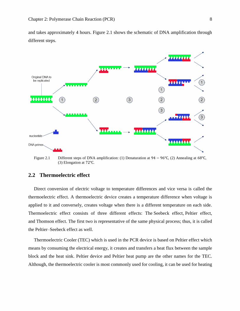
and takes approximately 4 hours. Figure 2.1 shows the schematic of DNA amplification through
different steps.
Figure 2.1 Different steps of DNA amplification: (1) Denaturation at 94 − 96, (2) Annealing at 68,
(3) Elongation at 72.
2.2 Thermoelectric effect
Direct conversion of electric voltage to temperature differences and vice versa is called the
thermoelectric effect. A thermoelectric device creates a temperature difference when voltage is
applied to it and conversely, creates voltage when there is a different temperature on each side.
Thermoelectric effect consists of three different effects: The Seebeck effect, Peltier effect,
and Thomson effect. The first two is representative of the same physical process; thus, it is called
the Peltier–Seebeck effect as well.
Thermoelectric Cooler (TEC) which is used in the PCR device is based on Peltier effect which
means by consuming the electrical energy, it creates and transfers a heat flux between the sample
block and the heat sink. Peltier device and Peltier heat pump are the other names for the TEC.
Although, the thermoelectric cooler is most commonly used for cooling, it can be used for heating

Chapter 2: Polymerase Chain Reaction (PCR) 9
as well. The thermoelectric cooler has both pros and cons. TECs are high-priced and have poor
efficiency while they have long life, small size and flexible shape.
Two different types of semiconductors, p-type and n-type, are used in TECs since they have
different electron densities. The semiconductors are placed electrically in series and thermally in
parallel to each other. They are joined with a thermally conducting plate on each side. A flow of
DC current is created across the junction of semiconductors, when a voltage is applied to the free
ends of the two semiconductors. This flow of current triggers a temperature difference. Heat is
absorbed by the cooling plate and then it is transferred to the side where the heat sink is located.
Two ceramic plates surround the TECs which are connected alongside. The number of TECs in
the system specifies the cooling ability of the total unit.
TECs have both advantages and disadvantages. Their pros are as follows:
They do not need frequent maintenance since they lack any moving parts.
They can have very small size as well as flexible shape.
Their temperature can be controlled precisely
They operate for a long time, usually their mean time between failures (MTBF) exceeds
100,000 hours.
They can be controlled by changing the input current/voltage.
Their Cons are:
They can only dissipate a limited amount of heat.
Their efficiency is low; hence, they waste a large amount of input electrical energy.
The amount of heat that can be absorbed by TEC is proportional to the current and time, and it
is obtained by the following relation:
𝑄 = 𝑃𝐼𝑡 2.1
where 𝑃 is the Peltier Coefficient, 𝐼 is the current, and 𝑡 is the time. The efficiency of TEC in
refrigeration cycle is around 10 − 15% of the ideal Carnot cycle refrigerator which is much lower
in comparison with 40 − 60% obtained by conventional compression cycle systems. As a result,
using thermoelectric cooling is only reasonable where its advantages such as low maintenance and
compact size outweigh its low efficiency.
Chapter 2: Polymerase Chain Reaction (PCR) 10
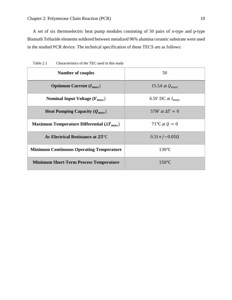
A set of six thermoelectric heat pump modules consisting of 50 pairs of n-type and p-type
Bismuth Telluride elements soldered between metalized 96% alumina ceramic substrate were used
in the studied PCR device. The technical specification of these TECS are as follows:
Table 2.1 Characteristics of the TEC used in this study
Number of couples 50
Optimum Current (𝑰𝒎𝒂𝒙) 15.5𝐴 at 𝑄𝑚𝑎𝑥
Nominal Input Voltage (𝑽𝒎𝒂𝒙) 6.5𝑉 DC at 𝐼𝑚𝑎𝑥
Heat Pumping Capacity (𝑸𝒎𝒂𝒙) 57𝑊 at ∆𝑇 = 0
Maximum Temperature Differential (∆𝑻𝒎𝒂𝒙) 71 at 𝑄 = 0
Ac Electrical Resistance at 𝟐𝟓 0.31+/−0.05Ω
Minimum Continuous Operating Temperature 130
Minimum Short-Term Process Temperature 150

11
Chapter 3: Numerical Model
Chapter 3: Numerical Model 12
3 Chapter 3: Numerical Model
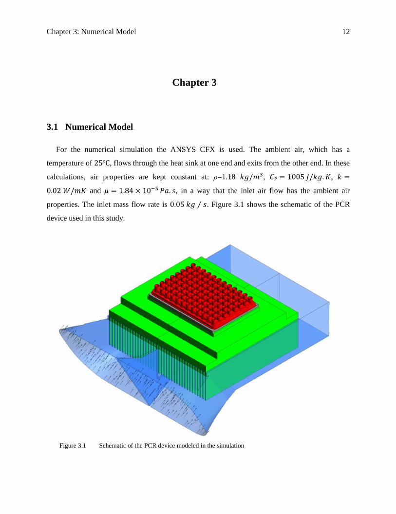
3.1 Numerical Model
For the numerical simulation the ANSYS CFX is used. The ambient air, which has a
temperature of 25, flows through the heat sink at one end and exits from the other end. In these
calculations, air properties are kept constant at: ρ=1.18 𝑘𝑔/𝑚3, 𝐶𝑝 = 1005 𝐽/𝑘𝑔. 𝐾, 𝑘 =
0.02 𝑊/𝑚𝐾 and 𝜇 = 1.84 × 10⁻⁵ 𝑃𝑎. 𝑠, in a way that the inlet air flow has the ambient air
properties. The inlet mass flow rate is 0.05 𝑘𝑔 ⁄ 𝑠. Figure 3.1 shows the schematic of the PCR
device used in this study.
Figure 3.1 Schematic of the PCR device modeled in the simulation
Chapter 3: Numerical Model 13
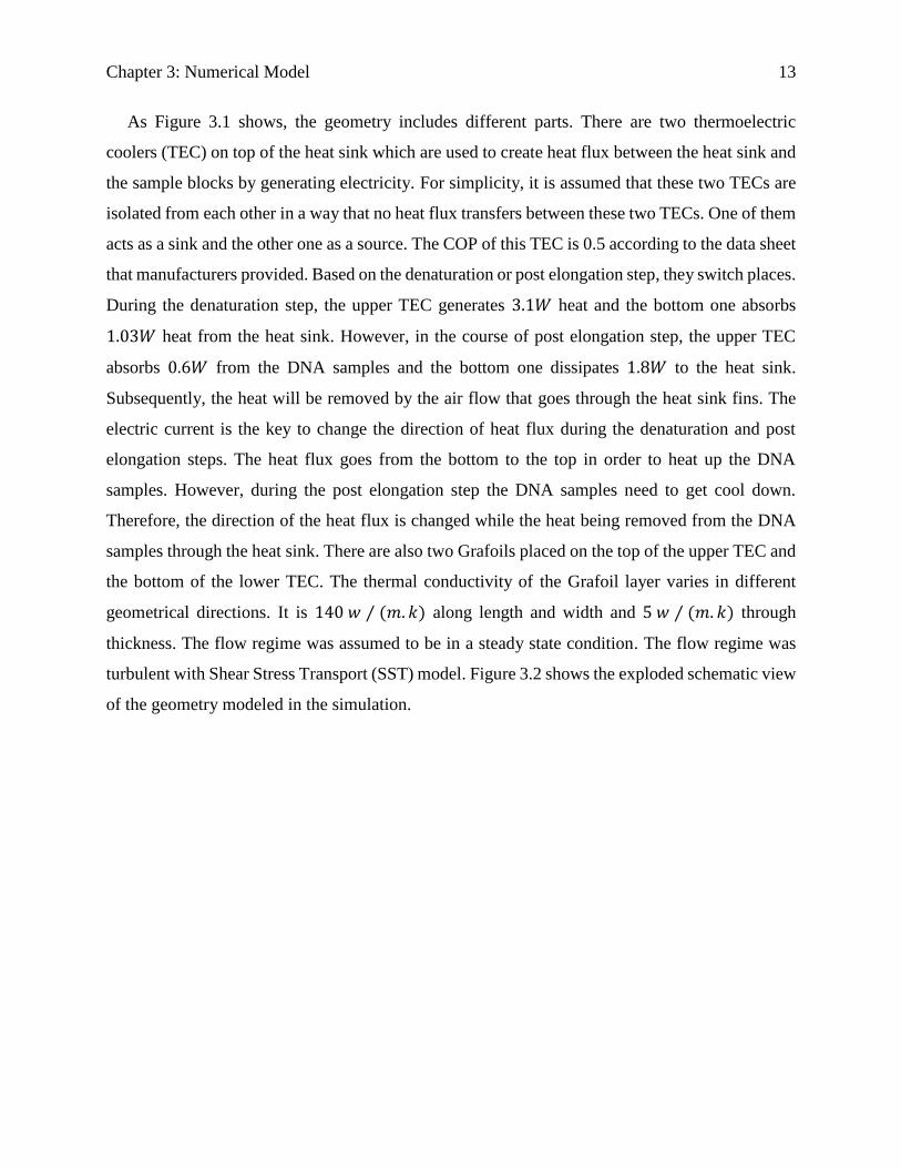
As Figure 3.1 shows, the geometry includes different parts. There are two thermoelectric
coolers (TEC) on top of the heat sink which are used to create heat flux between the heat sink and
the sample blocks by generating electricity. For simplicity, it is assumed that these two TECs are
isolated from each other in a way that no heat flux transfers between these two TECs. One of them
acts as a sink and the other one as a source. The COP of this TEC is 0.5 according to the data sheet
that manufacturers provided. Based on the denaturation or post elongation step, they switch places.
During the denaturation step, the upper TEC generates 3.1𝑊 heat and the bottom one absorbs
1.03𝑊 heat from the heat sink. However, in the course of post elongation step, the upper TEC
absorbs 0.6𝑊 from the DNA samples and the bottom one dissipates 1.8𝑊 to the heat sink.
Subsequently, the heat will be removed by the air flow that goes through the heat sink fins. The
electric current is the key to change the direction of heat flux during the denaturation and post
elongation steps. The heat flux goes from the bottom to the top in order to heat up the DNA
samples. However, during the post elongation step the DNA samples need to get cool down.
Therefore, the direction of the heat flux is changed while the heat being removed from the DNA
samples through the heat sink. There are also two Grafoils placed on the top of the upper TEC and
the bottom of the lower TEC. The thermal conductivity of the Grafoil layer varies in different
geometrical directions. It is 140 𝑤 ⁄ (𝑚. 𝑘) along length and width and 5 𝑤 ⁄ (𝑚. 𝑘) through
thickness. The flow regime was assumed to be in a steady state condition. The flow regime was
turbulent with Shear Stress Transport (SST) model. Figure 3.2 shows the exploded schematic view
of the geometry modeled in the simulation.
Chapter 3: Numerical Model 14
Figure 3.2 Computational domain of the PCR device modeled in the simulation
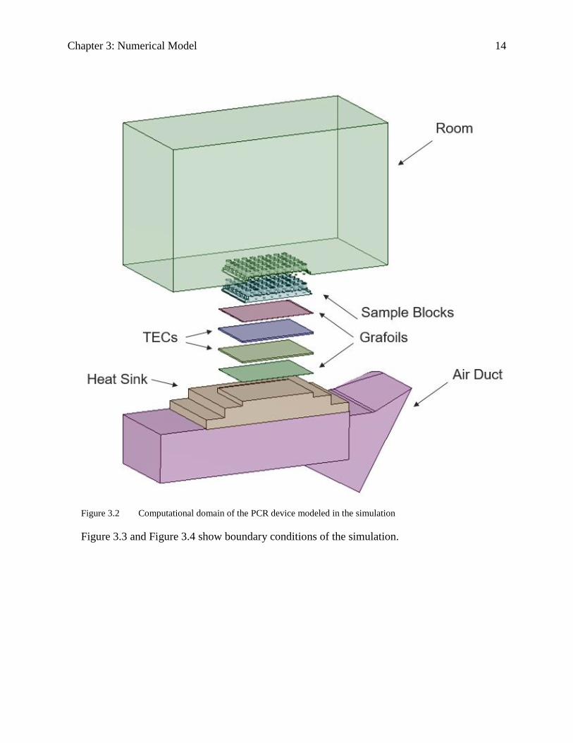
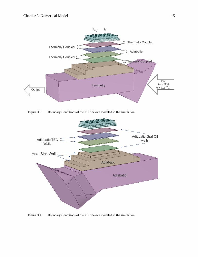
Figure 3.3 and Figure 3.4 show boundary conditions of the simulation.
Chapter 3: Numerical Model 15
Figure 3.3 Boundary Conditions of the PCR device modeled in the simulation
Figure 3.4 Boundary Conditions of the PCR device modeled in the simulation
Chapter 3: Numerical Model 16
3.2 Governing Equations
Assuming the flow to be Newtonian, incompressible, and in a steady state, the governing
equations would be as follows:
– Continuity Equation
∇. 𝑼 = 0 3.1
where 𝑼 is the velocity vector of the flow.
– Momentum Equation
𝜌𝑼. ∇(𝑼) = −∇𝑝 + 𝜇∇2𝑼 + 𝒇𝑏 3.2
where 𝒇𝑏 is a body force in – 𝑧 direction e.g. gravitational force and 𝑝 is the pressure.
– Energy Equation
∇. (𝜌𝑼𝑒) = ∇. (𝑘∇𝑇) + 𝑆𝐸 3.3
where 𝑆𝐸 is the heat source which comes from the TECs, explained and 𝑒 is internal energy.
Viscous dissipation is neglected. Additionally, Fourier’s law governs the heat conduction in solid
parts which is based on the following relation:
𝒒 = −𝑘∇𝑇 3.4
3.3 Mesh Independence Study
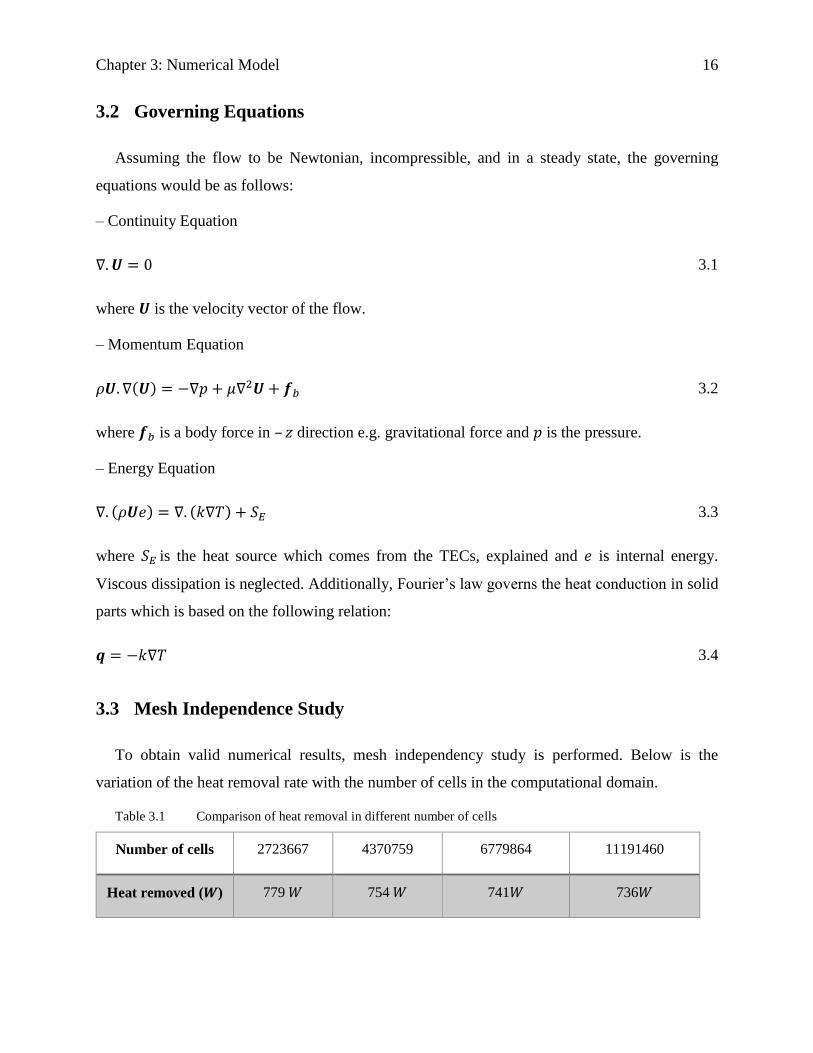
To obtain valid numerical results, mesh independency study is performed. Below is the
variation of the heat removal rate with the number of cells in the computational domain.
Table 3.1 Comparison of heat removal in different number of cells
Number of cells 2723667 4370759 6779864 11191460
Heat removed (𝑾) 779 𝑊 754 𝑊 741𝑊 736𝑊
Chapter 3: Numerical Model 17
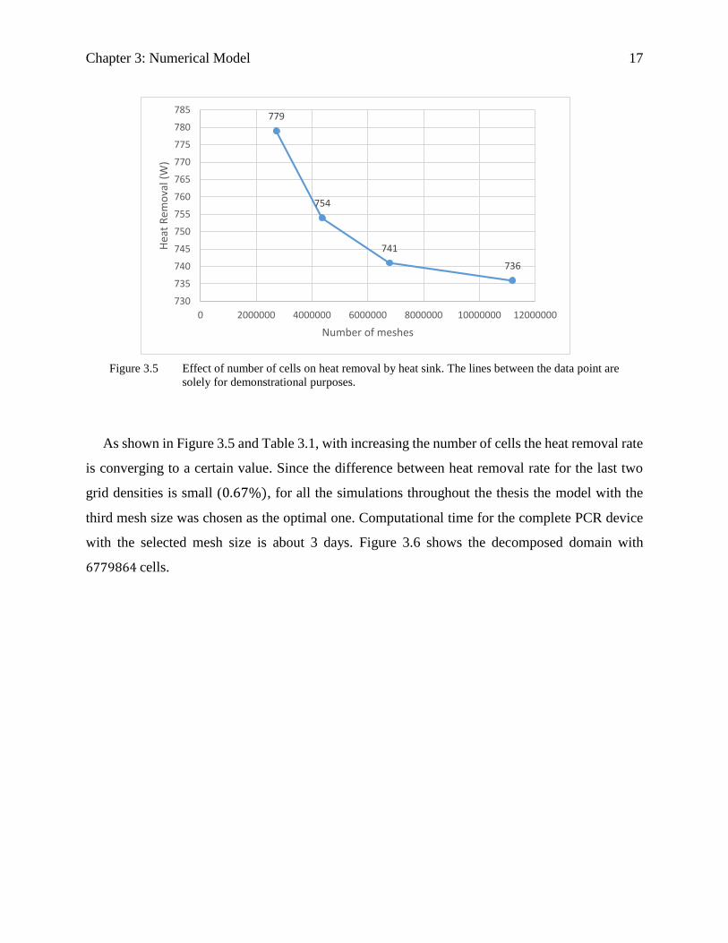
Figure 3.5 Effect of number of cells on heat removal by heat sink. The lines between the data point are
solely for demonstrational purposes.
As shown in Figure 3.5 and Table 3.1, with increasing the number of cells the heat removal rate
is converging to a certain value. Since the difference between heat removal rate for the last two
grid densities is small (0.67%), for all the simulations throughout the thesis the model with the
third mesh size was chosen as the optimal one. Computational time for the complete PCR device
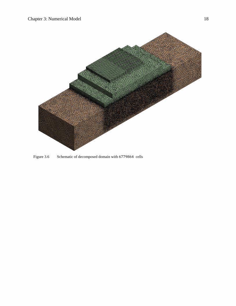
with the selected mesh size is about 3 days. Figure 3.6 shows the decomposed domain with
6779864 cells.
779
754
741
736
730
735
740
745
750
755
760
765
770
775
780
785
0 2000000 4000000 6000000 8000000 10000000 12000000
Hea
t R
emo
val (
W)
Number of meshes
Chapter 3: Numerical Model 18
Figure 3.6 Schematic of decomposed domain with 6779864 cells

19
Chapter 4: Numerical Results and
Discussion
Chapter 4: Numerical Results and Discussion 20
4 Chapter 4: Numerical Results and
Discussion
4.1 Results
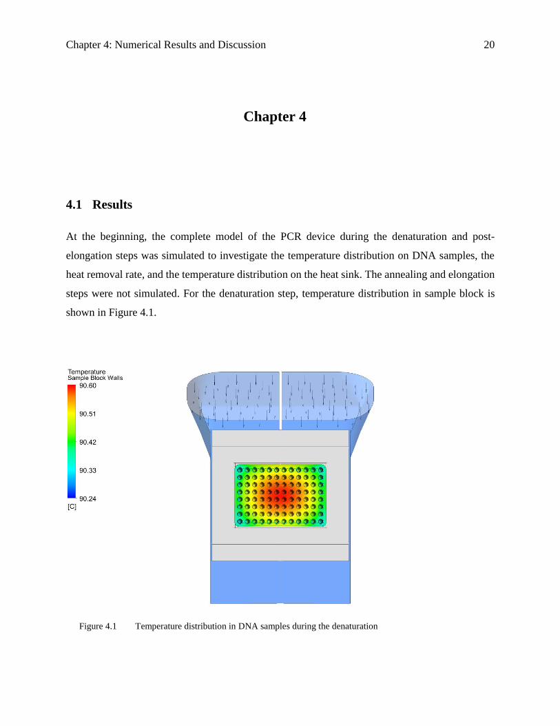
At the beginning, the complete model of the PCR device during the denaturation and post-
elongation steps was simulated to investigate the temperature distribution on DNA samples, the
heat removal rate, and the temperature distribution on the heat sink. The annealing and elongation
steps were not simulated. For the denaturation step, temperature distribution in sample block is
shown in Figure 4.1.
Figure 4.1 Temperature distribution in DNA samples during the denaturation

Chapter 4: Numerical Results and Discussion 21
The temperature uniformity of 0.36 was obtained on DNA samples. This temperature uniformity
is less than 0.8 which was obtained previously at Bio-Rad laboratories. This difference can be
due to the adiabatic boundary condition assigned to the common surface between the two TECs
leading to no heat being transferred between the upper and lower part of the model. Additionally,
simulation of post-elongation was carried out to study the effective parameters as well. The
temperature distribution in the post-elongation step is shown in Figure 4.2.
Figure 4.2 Temperature distribution in DNA sample during the post elongation
Temperature difference on DNA samples in the post elongation step was obtained to be
0.06. However, as it was mentioned before, there is no heat transfer between TECs. As a result,
the effect of fin length cannot be seen directly on the temperature distribution on DNA samples.
In this regard, TECs, Grafoils, and sample block were removed from the geometry to investigate
the effect of fin length on the heat removal rate by the heat sink. In this step, the simulation of air
duct and heat sink was done with different geometrical parameters in order to understand the effect
of fin length and the air gap below the heat sink.
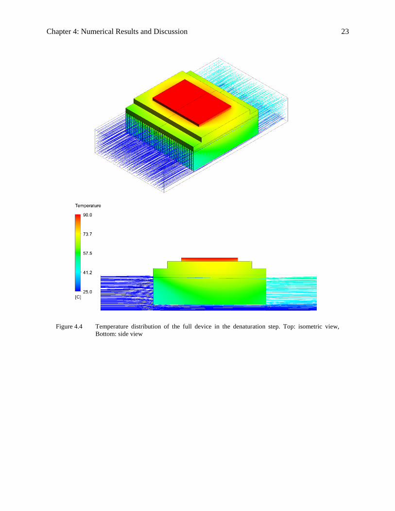
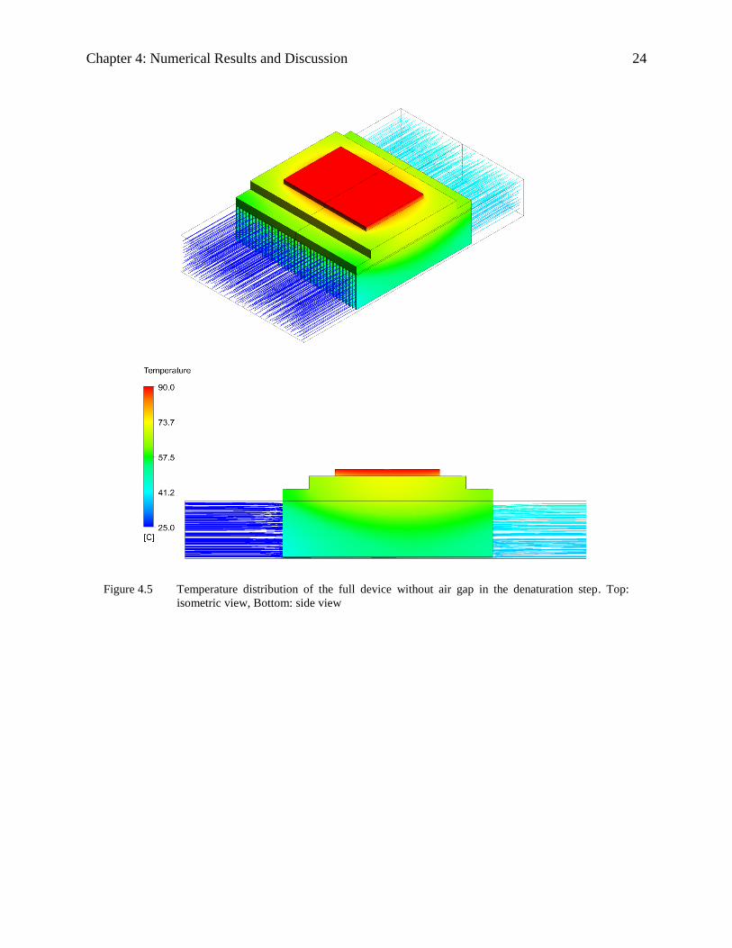
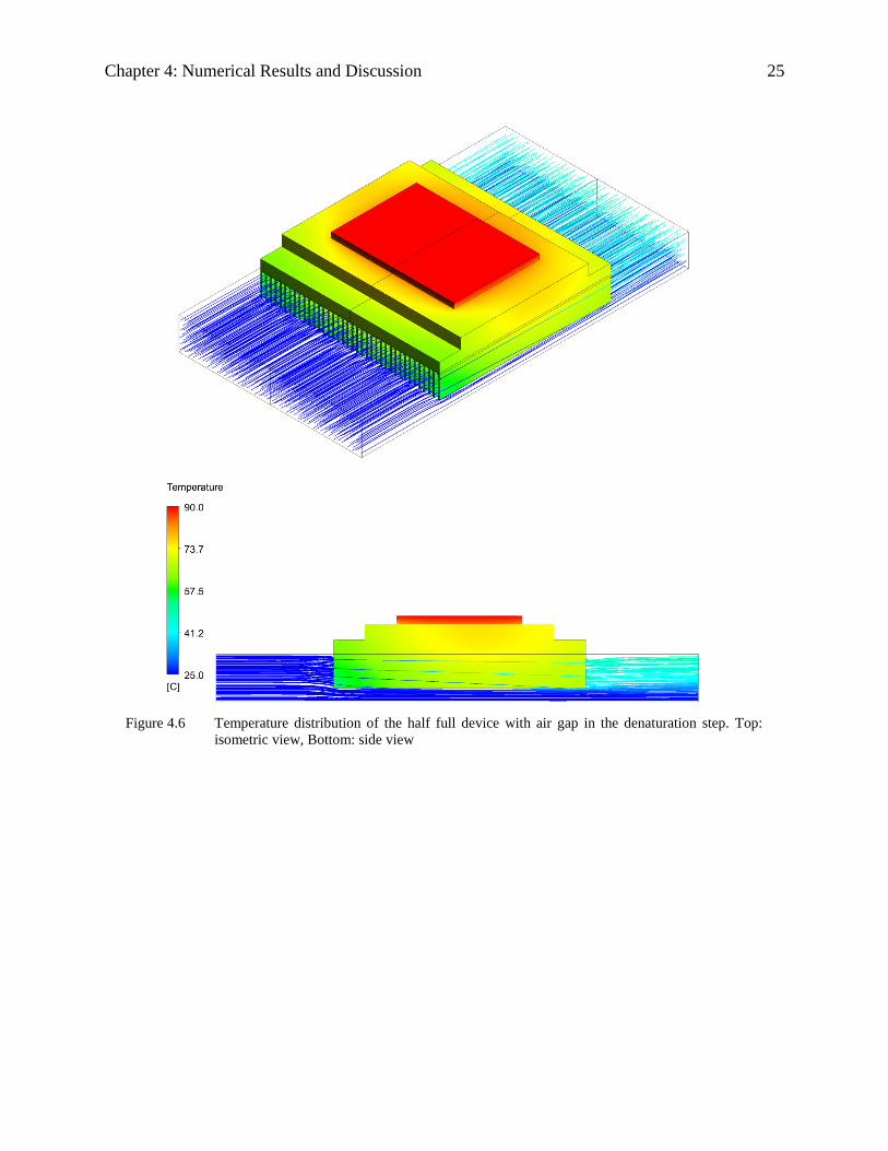
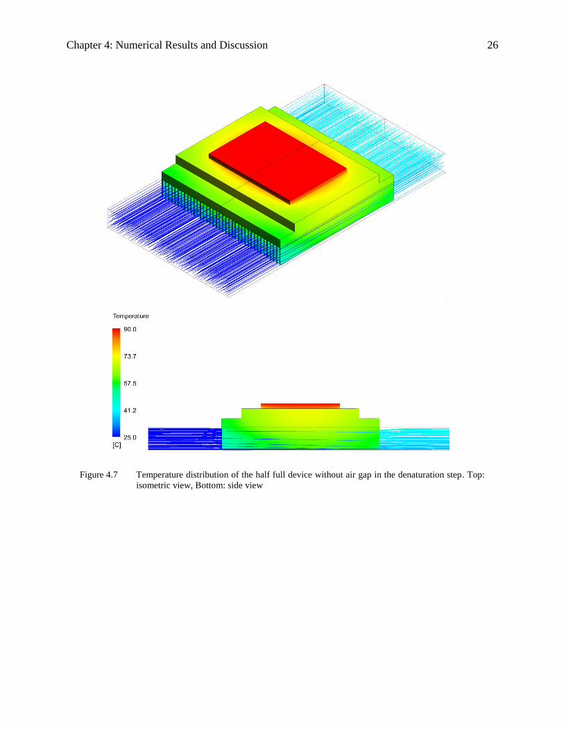
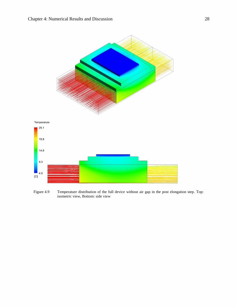
Initially, the complete geometry of heat sink and air duct was simulated. Later, the air gap
underneath the heatsink was removed to investigate how this gap affects the efficiency of the heat
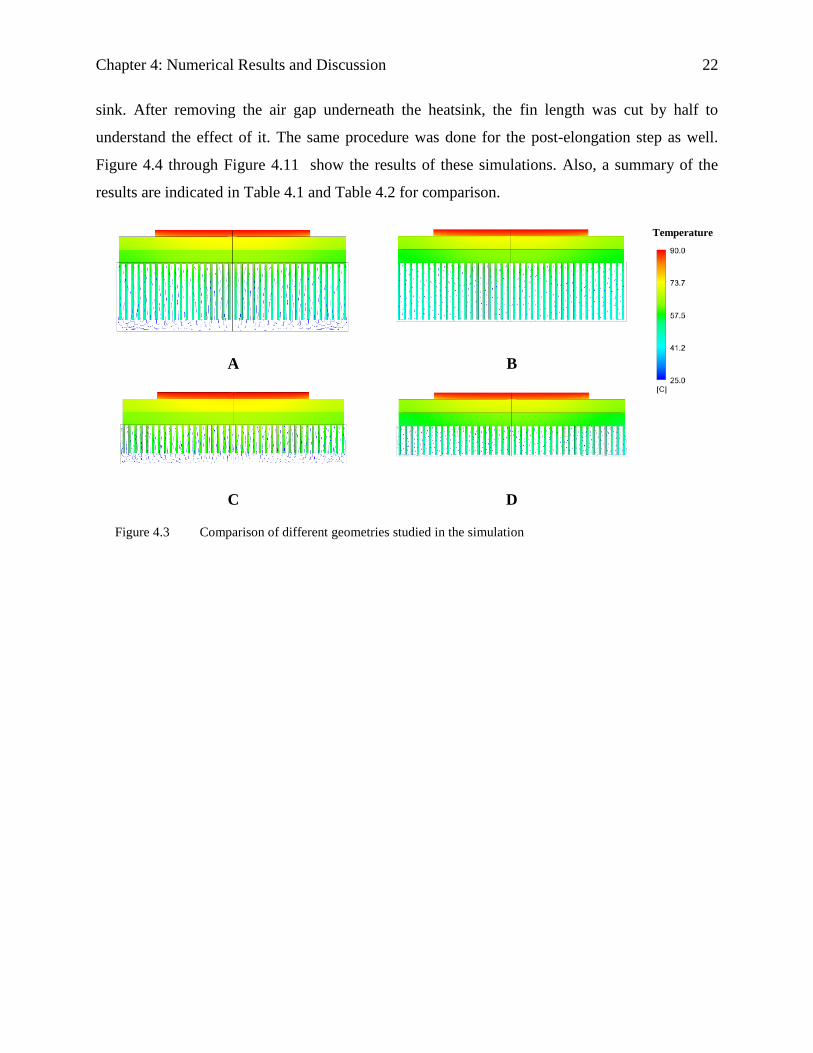
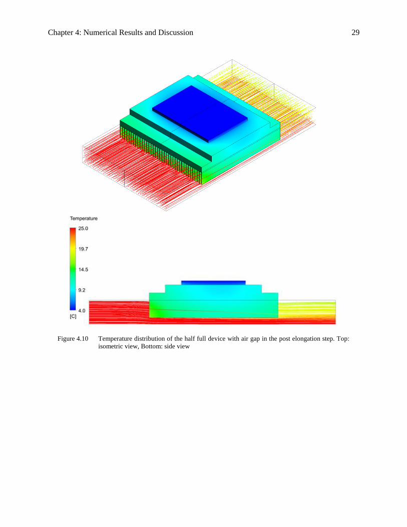
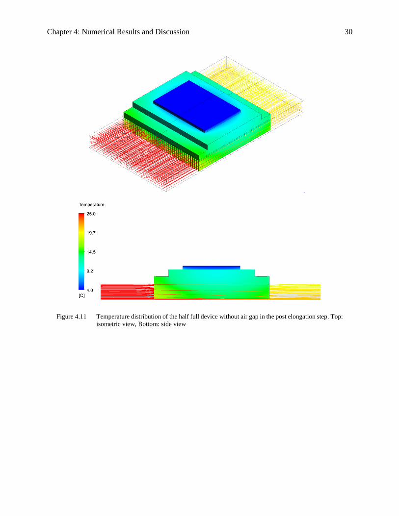
Chapter 4: Numerical Results and Discussion 22
sink. After removing the air gap underneath the heatsink, the fin length was cut by half to
understand the effect of it. The same procedure was done for the post-elongation step as well.
Figure 4.4 through Figure 4.11 show the results of these simulations. Also, a summary of the
results are indicated in Table 4.1 and Table 4.2 for comparison.
Temperature
A B
C D
Figure 4.3 Comparison of different geometries studied in the simulation
Chapter 4: Numerical Results and Discussion 23
Figure 4.4 Temperature distribution of the full device in the denaturation step. Top: isometric view,
Bottom: side view
Chapter 4: Numerical Results and Discussion 24
Figure 4.5 Temperature distribution of the full device without air gap in the denaturation step. Top:
isometric view, Bottom: side view
Chapter 4: Numerical Results and Discussion 25
Figure 4.6 Temperature distribution of the half full device with air gap in the denaturation step. Top:
isometric view, Bottom: side view
Chapter 4: Numerical Results and Discussion 26
Figure 4.7 Temperature distribution of the half full device without air gap in the denaturation step. Top:
isometric view, Bottom: side view
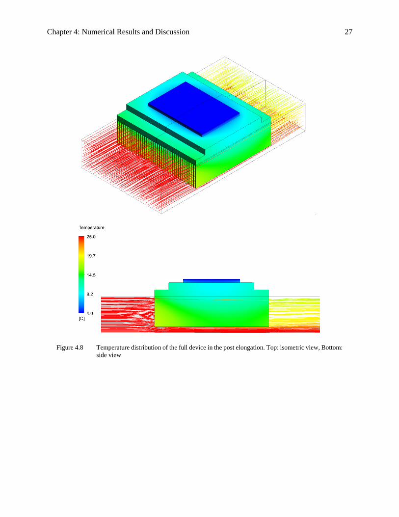
Chapter 4: Numerical Results and Discussion 27
Figure 4.8 Temperature distribution of the full device in the post elongation. Top: isometric view, Bottom:
side view
Chapter 4: Numerical Results and Discussion 28
Figure 4.9 Temperature distribution of the full device without air gap in the post elongation step. Top:
isometric view, Bottom: side view
Chapter 4: Numerical Results and Discussion 29
Figure 4.10 Temperature distribution of the half full device with air gap in the post elongation step. Top:
isometric view, Bottom: side view
Chapter 4: Numerical Results and Discussion 30
Figure 4.11 Temperature distribution of the half full device without air gap in the post elongation step. Top:
isometric view, Bottom: side view
Chapter 4: Numerical Results and Discussion 31
Table 4.1Table 4.2 illustrates air duct height, mass, and heat removal capacity of different heat
sink geometries.
Table 4.1 Comparison of different geometries of the heat sink in the denaturation step
Case A Case B Case C Case D
Air Duct Height 51mm 44mm (14% less) 30mm (42% less) 23mm (55% less)
Mass of Heat Sink 1.22kg 1.22kg 0.96kg (22% less) 0.96kg (22% less)
Heat added 741w 840w 648w 860w
Table 4.2 Comparison of different geometries of the heat sink in the post elongation step
Case A Case B Case C Case D
Air Duct Height 51mm 44mm(14% less) 30mm (42% less) 23mm (55% less)
Mass of Heat Sink 1.22kg 1.22kg 0.96kg (22% less) 0.96kg (22% less)
Heat removed 240w 270w 212w 274w
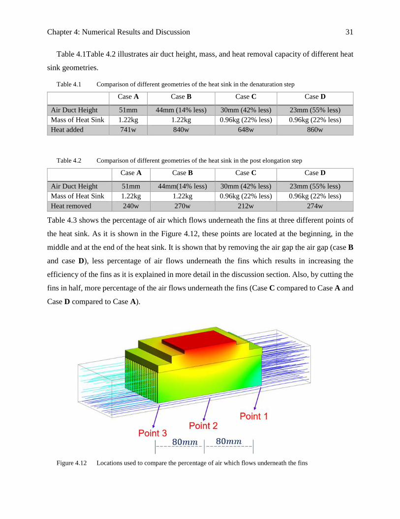
Table 4.3 shows the percentage of air which flows underneath the fins at three different points of
the heat sink. As it is shown in the Figure 4.12, these points are located at the beginning, in the
middle and at the end of the heat sink. It is shown that by removing the air gap the air gap (case B
and case D), less percentage of air flows underneath the fins which results in increasing the
efficiency of the fins as it is explained in more detail in the discussion section. Also, by cutting the
fins in half, more percentage of the air flows underneath the fins (Case C compared to Case A and
Case D compared to Case A).
Figure 4.12 Locations used to compare the percentage of air which flows underneath the fins
Chapter 4: Numerical Results and Discussion 32
Table 4.3 Amount of air which flows beneath the fins at three different locations
Point 1 Point 2 Point 3
Case A 22.6% 27.8% 28.7% Case B 4.3% 4.6% 4.3% Case C 36.8% 43.1% 45.5% Case D 8.6% 9.3% 8.7%
Table 4.4 compares the pressure difference between the inlet and outlet of the heat sink. As it
is illustrated in the table, by removing the air gap the pressure difference between the inlet and
outlet increases since most of the air flows through the fins. Moreover, by cutting the fins in half,
the air should flow through the thinner channel, which again, has the same result.
Table 4.4 Pressure drop between inlet and outlet of the heat sink
Pressure Gradient (𝑷𝒂)
Case A 175.2 Case B 293.3 Case C 372.5 Case D 976.4
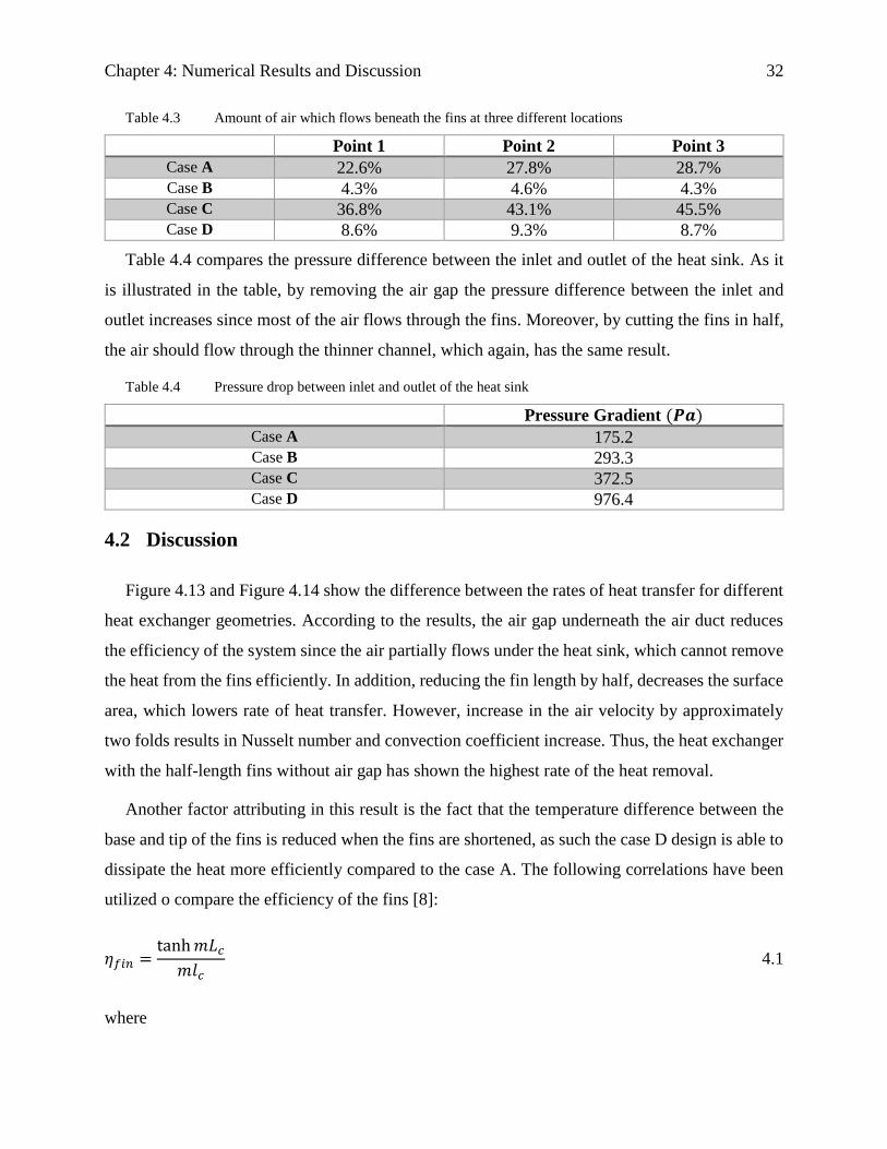
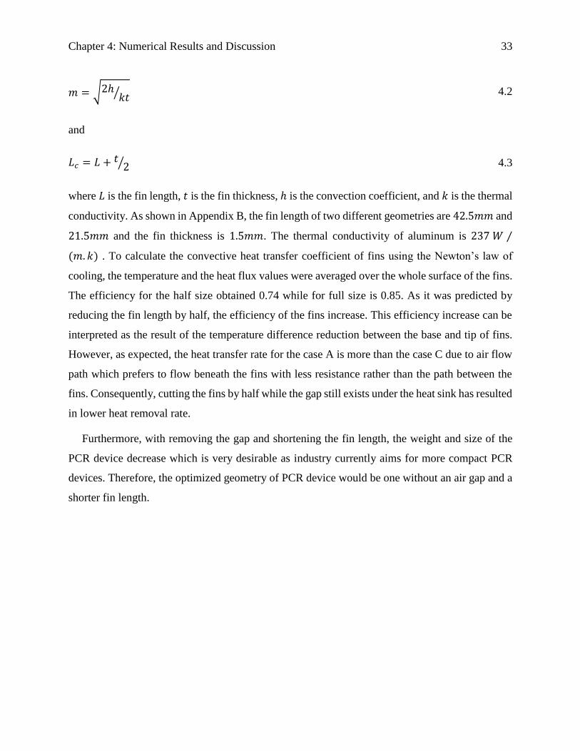
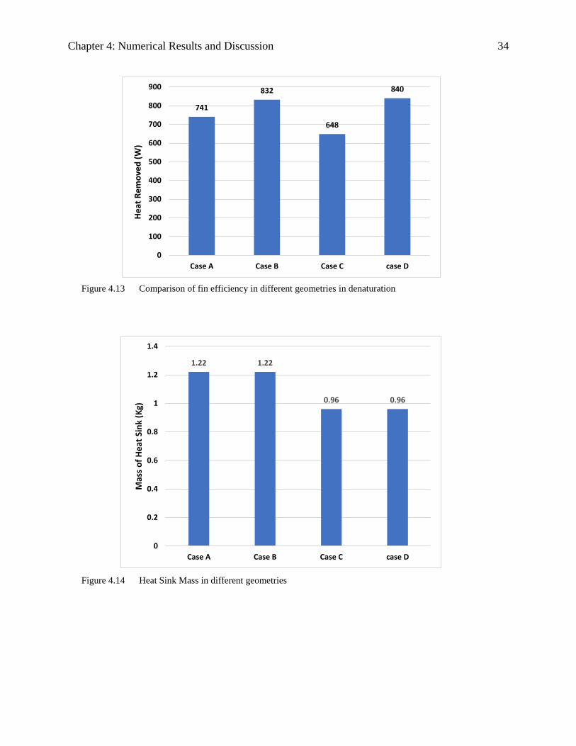
4.2 Discussion
Figure 4.13 and Figure 4.14 show the difference between the rates of heat transfer for different
heat exchanger geometries. According to the results, the air gap underneath the air duct reduces
the efficiency of the system since the air partially flows under the heat sink, which cannot remove
the heat from the fins efficiently. In addition, reducing the fin length by half, decreases the surface
area, which lowers rate of heat transfer. However, increase in the air velocity by approximately
two folds results in Nusselt number and convection coefficient increase. Thus, the heat exchanger
with the half-length fins without air gap has shown the highest rate of the heat removal.
Another factor attributing in this result is the fact that the temperature difference between the
base and tip of the fins is reduced when the fins are shortened, as such the case D design is able to
dissipate the heat more efficiently compared to the case A. The following correlations have been
utilized o compare the efficiency of the fins [8]:
𝜂𝑓𝑖𝑛 =tanh 𝑚𝐿𝑐
𝑚𝑙𝑐 4.1
where
Chapter 4: Numerical Results and Discussion 33
𝑚 = √2ℎ𝑘𝑡⁄ 4.2
and
𝐿𝑐 = 𝐿 + 𝑡2⁄ 4.3
where 𝐿 is the fin length, 𝑡 is the fin thickness, ℎ is the convection coefficient, and 𝑘 is the thermal
conductivity. As shown in Appendix B, the fin length of two different geometries are 42.5𝑚𝑚 and
21.5𝑚𝑚 and the fin thickness is 1.5𝑚𝑚. The thermal conductivity of aluminum is 237 𝑊 ⁄
(𝑚. 𝑘) . To calculate the convective heat transfer coefficient of fins using the Newton’s law of
cooling, the temperature and the heat flux values were averaged over the whole surface of the fins.
The efficiency for the half size obtained 0.74 while for full size is 0.85. As it was predicted by
reducing the fin length by half, the efficiency of the fins increase. This efficiency increase can be
interpreted as the result of the temperature difference reduction between the base and tip of fins.
However, as expected, the heat transfer rate for the case A is more than the case C due to air flow
path which prefers to flow beneath the fins with less resistance rather than the path between the
fins. Consequently, cutting the fins by half while the gap still exists under the heat sink has resulted
in lower heat removal rate.
Furthermore, with removing the gap and shortening the fin length, the weight and size of the
PCR device decrease which is very desirable as industry currently aims for more compact PCR
devices. Therefore, the optimized geometry of PCR device would be one without an air gap and a
shorter fin length.
Chapter 4: Numerical Results and Discussion 34
Figure 4.13 Comparison of fin efficiency in different geometries in denaturation
Figure 4.14 Heat Sink Mass in different geometries
741
832
648
840
0
100
200
300
400
500
600
700
800
900
Case A Case B Case C case D
He
at R
em
ove
d (
W)
1.22 1.22
0.96 0.96
0
0.2
0.4
0.6
0.8
1
1.2
1.4
Case A Case B Case C case D
Mas
s o
f H
eat
Sin
k (K
g)
35
Chapter 5: Metal Foam
Chapter 5: Metal Foam 36
5 Chapter 5: Metal Foam
5.1 Introduction
Metal foams are a group of porous material which have been widely used in different
applications for the past recent years. Their main characteristic that make them useful in heat
transfer applications is their large surface area to volume ratio which ranges from 200 𝑚^2 ⁄
𝑚^3 to 5000 𝑚^2 ⁄ 𝑚^3 [9, 10]. Due to this large specific surface area, metal foams are
excellent heat transfer medium. Metal foams are also known for another geometrical characteristic
which is their pore density. Pore density is defined as the number of pores per linear inch (PPI).
The range of porosity of metal foams is from 5 to 70 PPI for the commercially available ones.
Based on their structure, metal foams are divided into two different groups: closed-cell and
open-cell foams. Closed-cell foams have been used as an impact absorbing material which remain
deformed after the impact. Additionally, they are used as light weight structures in aerospace
industry. Open-cell metal foams, on the other hand, are newer and are mostly used in heat transfer
applications such as compact heat exchangers, combustors, biphasic cooling systems, energy
storage devices, spreaders, and heat sinks. Their vast applications in heat transfer is due to their
good thermo-physical properties such as high surface area to volume ratio that increases their
thermal conductivity. Open-cell metal foams are often made of copper, nickel, aluminum, nickel
alloys and stainless steel. They are very lightweight structures as they are highly porous with
porosities usually greater than 0.85 [10, 11].
5.2 Metal Foam Literature Review
Study of heat transfer and fluid flow through porous media dates back to the 19th century when
Darcy first established the fundamentals of flow in porous medium in 1856 [12]. His study was
based on water flow in packed beds. His results showed that there is a linear relationship between
Chapter 5: Metal Foam 37
the pressure drop in the columns of packed beds and the flow rate and viscosity of the fluid while
having an inverse relationship with permeability (K) of the porous material. As metal foams differ
from packed beds in terms of geometrical complexity and higher porosity, different flow relations
were needed to define flow regimes. In 1892 Lord Rayleigh [13] and years later Maxwell [14],
investigated heat transfer in porous media by estimating the effective thermal conductivity of
porous media analytically under stagnant flow condition.
Recently, there have been a number of experimental and numerical studies on fluid flow and
heat transfer in metal foams. Calmidi, Bhattacharya and Mahajan [15, 16] determined analytically
and experimentally the permeability (𝐾), effective thermal conductivity (𝑘𝑒) and inertial
coefficient (𝑓) of high porosity metal foams. Their experimental results were obtained in high
porosity ranging from 0.89 to 0.97 and indicated that inertial coefficient (𝑓) was dependent only
on porosity when permeability (𝐾) increases with pore diameter and porosity of the medium. Their
analytical study predicted that the effective thermal conductivity of the foam (𝑘𝑒) was independent
of pore density while it highly depends on porosity and the ratio of the cross sections of the fiber
and the intersection. In their analytical simulation, they modeled the complex geometry of metal
foams with two-dimensional array of hexagonal cells.
A theoretical model was developed by Du Plessis et al. [17] to estimate pressure drop in
Newtonian fluid flow in metal foams. This model assumes a Poiseuille flow through a simplistic
unit cell model of the foam. After extension of this model to the tetrakaidecahedron unit cell
representation, they predicted a pressure drop analytically in both Forchheimer and Darcy regimes.
From this discovery, they found out that there is not a linear relationship between the pressure
gradient and the flow rate for high Reynold numbers [18]. Bhattacharya et al. [13] revised the
value for tortuosity in Du Plessis’s model and developed new formula for the permeability and
Forchheimer coefficient in metal foams with porosities ranging from 0.85 to 0.97.
Bonnet et al. carried out a number of experiments on different metal foams such as copper,
nickel and nickel-chrome alloys for pore sizes (𝑑𝑝) ranging from 500 to 5000 𝜇𝑚 to investigate
the pressure drop of working fluids, i.e. air and water, to formulate the flow parameters based on
the morphology of metal foams [18-20]. Their results were in agreement with the Forchheimer
flow model and they concluded that permeability (𝑘) is proportional to the square of pore size
while inertial coefficient (𝐶𝐹) is inversely proportional to the pore size.
Chapter 5: Metal Foam 38
Boomsma et al. [9, 21, 22] ran an experiment on aluminum metal foams as compact heat
exchangers. They used aluminum block with the dimensions of 40 mm x 40 mm x 2 mm. Water
was used as a coolant which flowed through the aluminum foam. They put a constant heat flux on
the top of the aluminum foam. Their aluminum metal foam heat exchanger, while consuming the
same pumping power, generated two to three times lower thermal resistance than the best heat
exchangers available in the market. They also prepared a 3D numerical model to simulate the fluid
flow in metal foams using a tetrakaidecahedron unit cell representation. They obtained 25% lower
pressure drop compared with the experiments. One reason for this underestimation is that they
neglected wall effects in their simulations.
5.3 Pore Density and Porosity
There are two different ways to study transport phenomena in metal foams: micro (pore) level
and macro level. When analysis is focused on the micro level, there is a need to have a complete
understanding of the structure of metal foams. In this regard, the morphological model of the foam
needs to be understood. There are two different ways to obtain a model: a simplistic repetitive unit
cell representation of the foam or a real structural model attained by computer tomography (CT)
or X-ray radiography. The geometrical models can define structural characteristics such as: pore
size, fiber (ligament) size, surface area to volume ratio, porosity, fluid flow and heat transfer
properties of the foams (e.g., effective thermal conductivity and permeability) [23].
One of the main characteristics of metal foams is pore density. Pore density is defined as the
number of pores per linear inch (PPI). The open cell foam in this study has a pore density of 10
PPI. Since there is no complete control over the size of the bubbles in the foaming process, the
size of pores are not exactly equal to each other. However, according to the advances in the
manufacturing process, less variation in the pore size and shape of metal foams are expected. The
average pore diameter (𝑑𝑝) has an inverse relationship with the nominal pore density (PPI) as
shown below:
𝑑𝑝 =25.4𝑚𝑚
𝑃𝑃𝐼 5.1
Porosity (ε) is another physical property of the foams. It is defined as the volume of void divided
by the total volume of the foam,
Chapter 5: Metal Foam 39
𝜀 =𝑉𝑣𝑜𝑖𝑑
𝑉𝑡𝑜𝑡𝑎𝑙 5.2
Metal foams generally have a porosity ranging from 0.80 to 0.97. The foam that is used in this
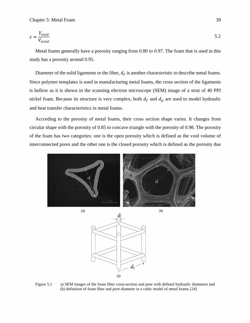
study has a porosity around 0.95.
Diameter of the solid ligaments or the fiber, 𝑑𝑓 is another characteristic to describe metal foams.
Since polymer templates is used in manufacturing metal foams, the cross section of the ligaments
is hollow as it is shown in the scanning electron microscope (SEM) image of a strut of 40 PPI
nickel foam. Because its structure is very complex, both 𝑑𝑓 and 𝑑𝑝 are used to model hydraulic
and heat transfer characteristics in metal foams.
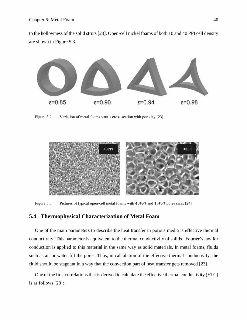
According to the porosity of metal foams, their cross section shape varies. It changes from
circular shape with the porosity of 0.85 to concave triangle with the porosity of 0.98. The porosity
of the foam has two categories: one is the open porosity which is defined as the void volume of
interconnected pores and the other one is the closed porosity which is defined as the porosity due
Figure 5.1 a) SEM images of the foam fiber cross-section and pore with defined hydraulic diameters and
(b) definition of foam fiber and pore diameter in a cubic model of metal foams [24]
Chapter 5: Metal Foam 40
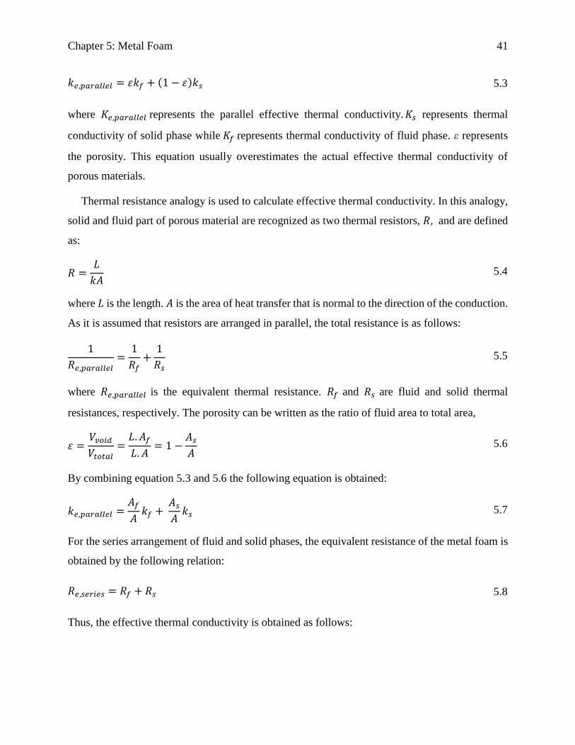
to the hollowness of the solid struts [23]. Open-cell nickel foams of both 10 and 40 PPI cell density
are shown in Figure 5.3.
Figure 5.2 Variation of metal foams strut’s cross section with porosity [23]
Figure 5.3 Pictures of typical open-cell metal foams with 40𝑃𝑃𝐼 and 10𝑃𝑃𝐼 pores sizes [24]
5.4 Thermophysical Characterization of Metal Foam
One of the main parameters to describe the heat transfer in porous media is effective thermal
conductivity. This parameter is equivalent to the thermal conductivity of solids. Fourier’s law for
conduction is applied to this material in the same way as solid materials. In metal foams, fluids
such as air or water fill the pores. Thus, in calculation of the effective thermal conductivity, the
fluid should be stagnant in a way that the convection part of heat transfer gets removed [23].
One of the first correlations that is derived to calculate the effective thermal conductivity (ETC)
is as follows [23]:
Chapter 5: Metal Foam 41
𝑘𝑒,𝑝𝑎𝑟𝑎𝑙𝑙𝑒𝑙 = 𝜀𝑘𝑓 + (1 − 𝜀)𝑘𝑠 5.3
where 𝐾𝑒,𝑝𝑎𝑟𝑎𝑙𝑙𝑒𝑙 represents the parallel effective thermal conductivity. 𝐾𝑠 represents thermal
conductivity of solid phase while 𝐾𝑓 represents thermal conductivity of fluid phase. ε represents
the porosity. This equation usually overestimates the actual effective thermal conductivity of
porous materials.
Thermal resistance analogy is used to calculate effective thermal conductivity. In this analogy,
solid and fluid part of porous material are recognized as two thermal resistors, 𝑅, and are defined
as:
𝑅 =𝐿
𝑘𝐴 5.4
where 𝐿 is the length. 𝐴 is the area of heat transfer that is normal to the direction of the conduction.
As it is assumed that resistors are arranged in parallel, the total resistance is as follows:
1
𝑅𝑒,𝑝𝑎𝑟𝑎𝑙𝑙𝑒𝑙=
1
𝑅𝑓+
1
𝑅𝑠 5.5
where 𝑅𝑒,𝑝𝑎𝑟𝑎𝑙𝑙𝑒𝑙 is the equivalent thermal resistance. 𝑅𝑓 and 𝑅𝑠 are fluid and solid thermal
resistances, respectively. The porosity can be written as the ratio of fluid area to total area,
𝜀 =𝑉𝑣𝑜𝑖𝑑
𝑉𝑡𝑜𝑡𝑎𝑙=
𝐿. 𝐴𝑓
𝐿. 𝐴= 1 −
𝐴𝑠
𝐴 5.6
By combining equation 5.3 and 5.6 the following equation is obtained:
𝑘𝑒,𝑝𝑎𝑟𝑎𝑙𝑙𝑒𝑙 =𝐴𝑓
𝐴𝑘𝑓 +
𝐴𝑠
𝐴𝑘𝑠 5.7
For the series arrangement of fluid and solid phases, the equivalent resistance of the metal foam is
obtained by the following relation:
𝑅𝑒,𝑠𝑒𝑟𝑖𝑒𝑠 = 𝑅𝑓 + 𝑅𝑠 5.8
Thus, the effective thermal conductivity is obtained as follows:
Chapter 5: Metal Foam 42
𝑘𝑒,𝑠𝑒𝑟𝑖𝑒𝑠 = (𝐿𝑓
𝐿
1
𝑘𝑓+
𝐿𝑠
𝐿
1
𝑘𝑠)
−1
5.9
The porosity in series arrangement can be written as:
𝜀 =𝐿𝑓 . 𝐴
𝐿. 𝐴= 1 −
𝐿𝑠
𝐿 5.10
As a result, the ETC in a series arrangement is obtained according to the following equation:
𝑘𝑒,𝑠𝑒𝑟𝑖𝑒𝑠 = (𝜀
𝑘𝑓+
1 − 𝜀
𝑘𝑠)
−1
5.11
This relation results in maximum resistance or minimum effective thermal conductivity. However,
in reality the metal foam material has neither parallel nor series arrangement. Therefore, their ETC
is between these two boundaries: the upper boundary which is in parallel arrangement and the
lower boundary which is in series.
Fluid flow through porous media was developed by Darcy when he started working on water
flow through beds of sands. He observed a linear relationship between pressure drop and flow rate
[12]. Later on, the fluid flow through metallic foams was characterized similarly. Thus, its pressure
gradient varies linearly with velocity and it is obtained from:
𝑑𝑝
𝑑𝑥=
𝜇
𝐾𝑢 5.12
where 𝜇 is dynamic viscosity and 𝐾 is permeability of metal foam. However, at higher velocities
deviation from Darcy law occurs as inertial effect becomes important [24]. Thus, the Dupuit–
Forchheimer modification is employed where a quadratic term in the expression for pressure
gradient is introduced [9].
𝑑𝑝
𝑑𝑥=
𝜇
𝐾𝑢 +
𝜌𝐶𝐹
√𝐾𝑢2 5.13
As stated above, in order to use the Darcy law, first the regime of the flow should be defined
by the Reynolds number. Hydraulic diameter of the channel can be used as the length scale for
Reynolds number definition. Therefore, Reynolds number is obtained from
Chapter 5: Metal Foam 43
𝑅𝑒 =𝜌𝑢𝑑ℎ
𝜇 5.14
Where 𝜌 is the density of the fluid flow, 𝑢 is the velocity of the flow, 𝜇 is the dynamic viscosity
of the fluid, and 𝑑ℎis the hydraulic diameter of the air duct channel which is obtained from
𝑑ℎ =4𝐴
𝑃 5.15
where 𝐴 is the cross-sectional area, and 𝑃 is the wetted perimeter of the cross-section
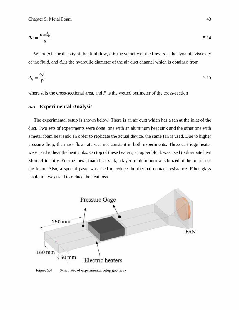
5.5 Experimental Analysis
The experimental setup is shown below. There is an air duct which has a fan at the inlet of the
duct. Two sets of experiments were done: one with an aluminum heat sink and the other one with
a metal foam heat sink. In order to replicate the actual device, the same fan is used. Due to higher
pressure drop, the mass flow rate was not constant in both experiments. Three cartridge heater
were used to heat the heat sinks. On top of these heaters, a copper block was used to dissipate heat
More efficiently. For the metal foam heat sink, a layer of aluminum was brazed at the bottom of
the foam. Also, a special paste was used to reduce the thermal contact resistance. Fiber glass
insulation was used to reduce the heat loss.
Figure 5.4 Schematic of experimental setup geometry
Chapter 5: Metal Foam 44
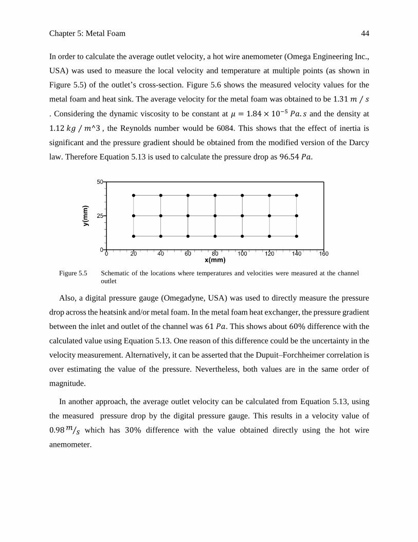
In order to calculate the average outlet velocity, a hot wire anemometer (Omega Engineering Inc.,
USA) was used to measure the local velocity and temperature at multiple points (as shown in
Figure 5.5) of the outlet’s cross-section. Figure 5.6 shows the measured velocity values for the
metal foam and heat sink. The average velocity for the metal foam was obtained to be 1.31 𝑚 ⁄ 𝑠
. Considering the dynamic viscosity to be constant at 𝜇 = 1.84 × 10⁻⁵ 𝑃𝑎. 𝑠 and the density at
1.12 𝑘𝑔 ⁄ 𝑚^3 , the Reynolds number would be 6084. This shows that the effect of inertia is
significant and the pressure gradient should be obtained from the modified version of the Darcy
law. Therefore Equation 5.13 is used to calculate the pressure drop as 96.54 𝑃𝑎.
Figure 5.5 Schematic of the locations where temperatures and velocities were measured at the channel
outlet
Also, a digital pressure gauge (Omegadyne, USA) was used to directly measure the pressure
drop across the heatsink and/or metal foam. In the metal foam heat exchanger, the pressure gradient
between the inlet and outlet of the channel was 61 𝑃𝑎. This shows about 60% difference with the
calculated value using Equation 5.13. One reason of this difference could be the uncertainty in the
velocity measurement. Alternatively, it can be asserted that the Dupuit–Forchheimer correlation is
over estimating the value of the pressure. Nevertheless, both values are in the same order of
magnitude.
In another approach, the average outlet velocity can be calculated from Equation 5.13, using
the measured pressure drop by the digital pressure gauge. This results in a velocity value of
0.98 𝑚𝑠⁄ which has 30% difference with the value obtained directly using the hot wire
anemometer.
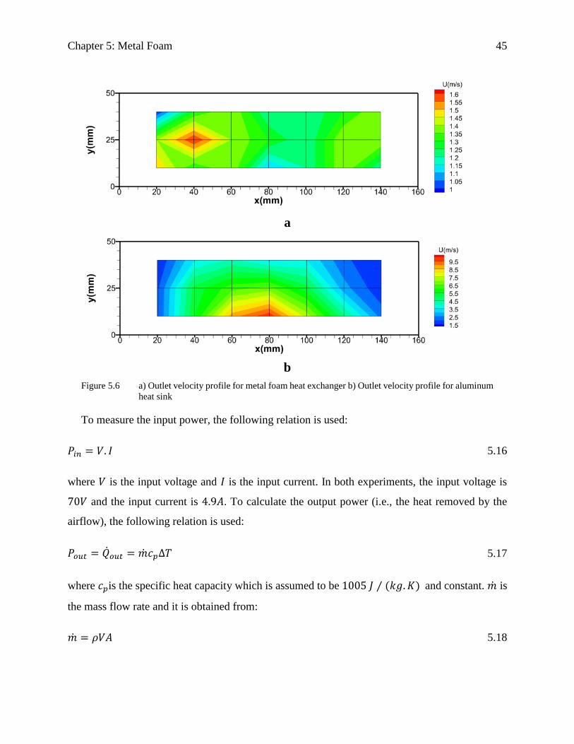
Chapter 5: Metal Foam 45
a
b
Figure 5.6 a) Outlet velocity profile for metal foam heat exchanger b) Outlet velocity profile for aluminum
heat sink
To measure the input power, the following relation is used:
𝑃𝑖𝑛 = 𝑉. 𝐼 5.16
where 𝑉 is the input voltage and 𝐼 is the input current. In both experiments, the input voltage is
70𝑉 and the input current is 4.9𝐴. To calculate the output power (i.e., the heat removed by the
airflow), the following relation is used:
𝑃𝑜𝑢𝑡 = 𝑜𝑢𝑡 = 𝑐𝑝∆𝑇 5.17
where 𝑐𝑝is the specific heat capacity which is assumed to be 1005 𝐽 ⁄ (𝑘𝑔. 𝐾) and constant. is
the mass flow rate and it is obtained from:
= 𝜌𝑉𝐴 5.18
Chapter 5: Metal Foam 46
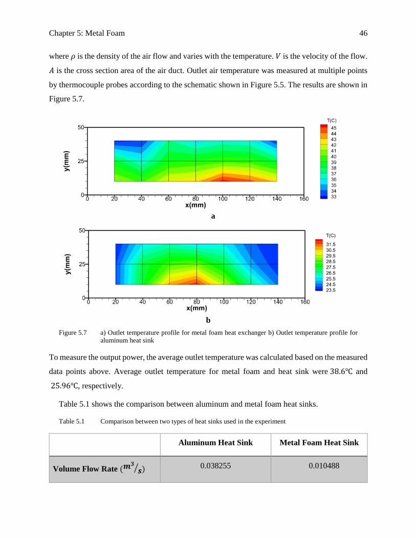
where 𝜌 is the density of the air flow and varies with the temperature. 𝑉 is the velocity of the flow.
𝐴 is the cross section area of the air duct. Outlet air temperature was measured at multiple points
by thermocouple probes according to the schematic shown in Figure 5.5. The results are shown in
Figure 5.7.
a
b
Figure 5.7 a) Outlet temperature profile for metal foam heat exchanger b) Outlet temperature profile for
aluminum heat sink
To measure the output power, the average outlet temperature was calculated based on the measured
data points above. Average outlet temperature for metal foam and heat sink were 38.6 and
25.96, respectively.
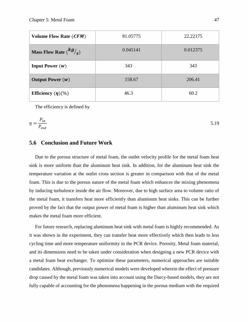
Table 5.1 shows the comparison between aluminum and metal foam heat sinks.
Table 5.1 Comparison between two types of heat sinks used in the experiment
Aluminum Heat Sink Metal Foam Heat Sink
Volume Flow Rate (𝒎𝟑
𝒔⁄ ) 0.038255 0.010488
Chapter 5: Metal Foam 47
Volume Flow Rate (𝑪𝑭𝑴) 81.05775 22.22175
Mass Flow Rate (𝒌𝒈
𝒔⁄ ) 0.045141 0.012375
Input Power (𝒘) 343 343
Output Power (𝒘) 158.67 206.41
Efficiency (𝜼)(%) 46.3 60.2
The efficiency is defined by
𝜂 =𝑃𝑖𝑛
𝑃𝑜𝑢𝑡 5.19
5.6 Conclusion and Future Work
Due to the porous structure of metal foam, the outlet velocity profile for the metal foam heat
sink is more uniform than the aluminum heat sink. In addition, for the aluminum heat sink the
temperature variation at the outlet cross section is greater in comparison with that of the metal
foam. This is due to the porous nature of the metal foam which enhances the mixing phenomena
by inducing turbulence inside the air flow. Moreover, due to high surface area to volume ratio of
the metal foam, it transfers heat more efficiently than aluminum heat sinks. This can be further
proved by the fact that the output power of metal foam is higher than aluminum heat sink which
makes the metal foam more efficient.
For future research, replacing aluminum heat sink with metal foam is highly recommended. As
it was shown in the experiment, they can transfer heat more effectively which then leads to less
cycling time and more temperature uniformity in the PCR device. Porosity, Metal foam material,
and its dimensions need to be taken under consideration when designing a new PCR device with
a metal foam heat exchanger. To optimize these parameters, numerical approaches are suitable
candidates. Although, previously numerical models were developed wherein the effect of pressure
drop caused by the metal foam was taken into account using the Darcy-based models, they are not
fully capable of accounting for the phenomena happening in the porous medium with the required

Chapter 5: Metal Foam 48
detail. As a result, developing more advanced numerical models capable of considering the effects
of pore size, struts, surface roughness, etc. is crucial. Some probable challenges accompanied with
such models could be increased number of computational cells (and as a result CPU time),
consistency between the geometrical model and the metal foam, numerical stability, etc.
49
6 References
1. Mahjoob, S., K. Vafai, and N.R. Beer, Rapid microfluidic thermal cycler for polymerase
chain reaction nucleic acid amplification. International Journal of Heat and Mass Transfer,
2008. 51(9–10): p. 2109-2122.
2. Yoon, D.S., et al., Precise temperature control and rapid thermal cycling in a
micromachined DNA polymerase chain reaction chip. Journal of Micromechanics and
microengineering, 2002. 12(6): p. 813.
3. Khandurina, J., et al., Integrated system for rapid PCR-based DNA analysis in microfluidic
devices. Analytical Chemistry, 2000. 72(13): p. 2995-3000.
4. Hsieh, T.-M., et al., Enhancement of thermal uniformity for a microthermal cycler and its
application for polymerase chain reaction. Sensors and Actuators B: Chemical, 2008.
130(2): p. 848-856.
5. Hu, G., et al., Electrokinetically controlled real-time polymerase chain reaction in
microchannel using Joule heating effect. Analytica Chimica Acta, 2006. 557(1–2): p. 146-
151.
6. Zhang, C. and D. Xing, Parallel DNA amplification by convective polymerase chain
reaction with various annealing temperatures on a thermal gradient device. Analytical
Biochemistry, 2009. 387(1): p. 102-112.
7. Janak, S. and E. Mayang, PCR thermal management in an integrated Lab on Chip. Journal
of Physics: Conference Series, 2006. 34(1): p. 222.
8. Cengel, Y.A. and A. Ghajar, Heat and mass transfer (a practical approach, SI version).
2011, McGraw-Hill Education.
9. Boomsma, K., D. Poulikakos, and F. Zwick, Metal foams as compact high performance
heat exchangers. Mechanics of materials, 2003. 35(12): p. 1161-1176.
10. Lu, T., H. Stone, and M. Ashby, Heat transfer in open-cell metal foams. Acta Materialia,
1998. 46(10): p. 3619-3635.
11. Ashby, M.F., et al., Metal foams: a design guide. 2000: Elsevier.
12. Darcy, H., Les fontaines publiques de la ville de Dijon: exposition et application. 1856:
Victor Dalmont.
13. Rayleigh, L., LVI. On the influence of obstacles arranged in rectangular order upon the
properties of a medium. The London, Edinburgh, and Dublin Philosophical Magazine and
Journal of Science, 1892. 34(211): p. 481-502.
14. Maxwell, J.C., A Treatise on Electricity and Magnetism Unabridged. 1954: Dover.
50
15. Bhattacharya, A., V. Calmidi, and R. Mahajan, Thermophysical properties of high porosity
metal foams. International Journal of Heat and Mass Transfer, 2002. 45(5): p. 1017-1031.
16. Calmidi, V. and R. Mahajan, Forced convection in high porosity metal foams.
TRANSACTIONS-AMERICAN SOCIETY OF MECHANICAL ENGINEERS
JOURNAL OF HEAT TRANSFER, 2000. 122(3): p. 557-565.
17. Du Plessis, P., et al., Pressure drop prediction for flow through high porosity metallic
foams. Chemical Engineering Science, 1994. 49(21): p. 3545-3553.
18. Bonnet, J.-P., F. Topin, and L. Tadrist, Flow laws in metal foams: compressibility and pore
size effects. Transport in Porous Media, 2008. 73(2): p. 233-254.
19. Bonnet, J., F. Topin, and L. Tadrist. Experimental study of two phase flow through open-
celled metallic foam. in Proceedings of the fifth international conference on porous metals
and metal foaming technology, Montreal. 2008.
20. Topin, F., et al., Experimental analysis of multiphase flow in metallic foam: flow laws, heat
transfer and convective boiling. Advanced Engineering Materials, 2006. 8(9): p. 890-899.
21. Poulikakos, D., The effects of compression and pore size variations on the liquid flow
characteristics in metal foams. Journal of fluids engineering, 2002. 124: p. 263-272.
22. Boomsma, K., D. Poulikakos, and Y. Ventikos, Simulations of flow through open cell metal
foams using an idealized periodic cell structure. International Journal of Heat and Fluid
Flow, 2003. 24(6): p. 825-834.
23. Taheri, M., Analytical and Numerical Modeling of Fluid Flow and Heat Transfer Through
Open-Cell Metal Foam Heat Exchangers. 2015, University of Toronto.
24. Tsolas, N. and S. Chandra, Forced Convection Heat Transfer in Spray Formed Copper and
Nickel Foam Heat Exchanger Tubes. Journal of heat transfer, 2012. 134(6): p. 062602.