optimization of large join queries: combining heuristics and combinatorial techniques

Optimization of Large Join Queries: Combining Heuristics and Combinatorial Techniques

Arun Swami

Computer Science Department, Stanford University, Stanford, CA 94305

Abstract We investigate the use of heuristics in optimizing queries with a large number of joins. Examples of such heuristics are the augmentation and local improvement heuristics described in this paper and a heuristic proposed by Krishnamurthy et al. We also study the combination of these heuristics with two general combinatorial optimization techniques, iterative improvement and simulated annealing, that were studied in a previous paper. Several interesting combinations are experimentally compared. For completeness, we also include simple iterative improvement and simulated annealing in our experimental comparisons. We find that two combinations of the augmentation heuristic and iterative improvement perform the best under most conditions. The results are validated using two different cost models and several different synthetic benchmarks.

1 Introduction Much effort has been devoted to developing good plans for executing queries in relational database systems [JK84]. These plans are termed query evaluation plans (QEPs). The techniques employed in current query optimizers assume that the queries to be processed involve a small number of joins (less than 10 joins). For example, the dynamic pro- gramming algorithm described in System/R [SAC+791 has a worst case time complexity of O(2N) (with an exponen- tial space requirement), where N is the number of joins. As N becomes larger than 10, use of this algorithm becomes infeasible.

We expect that some future applications built on top of relational systems will require processing of queries with a much larger number of joins. Krishnamurthy, Boral, and Zaniolo in [KBZ86] mention applications from logic pro- gramming resulting in “ . . . expressions (similar to database queries) with hundreds (if not thousands) of joins.” Object- oriented database systems, for instance, Iris [FBC+87],

Permission to copy without fee all or part of this material is granted provided that

the copies are not made or distributed for direct commercial advantage, the ACM

copyright notice and the title of the publication and its date appear, and notice is given that copying is by permission of the Association for Computing Machinery.

To copy otherwise, or to republish, requires a fee and/or specific pemksion. 0 1989 ACM o-89791-317-5/89/0005/0367 $1.50

that use relational systems for storage of information are another class of potential applications generating many joins. Finally, the use of views in relational systems can lead to an increase in the number of joins in the query being processed without the user being aware of it.

The fundamental problem with optimizing large join queries is searching the large spaces of possible QEPs or solutions. In [IW87], Ioannidis and Wong study how simulated annealing can be used to obtain an efficient algebraic structure for a given recursive query. This too is a problem that involves searching a large solution space. How- ever, they do not consider the problem of optimizing nonrecursive queries with a large number of joins.

In [KBZSS], Krishnamurthy, Boral, and Zaniolo described an O(N2) heuristic for optimizing non-recursive queries. This is one of the heuristics being compared in this paper. However, one should note that the theory on which their work is based requires that the cost functions have a certain form. All join methods do not have a cost function of the required form. Our work does not depend on using any particular cost model; any reasonable cost model will do. In fact, we present results for two different cost models: one for join processing in memory resident databases [Swa89a], and the other for disk based databases (similar to the model in [Bra84]).

In [SG88], Swami and Gupta addressed the problem of optimizing non-recursive large join queries (to be denoted as LJQOP). They showed that this problem is an NP-complete combinatorial optimization problem. They then discussed how general combinatorial optimization techniques such as iterative improvement and simulated annealing can be applied to LJQOP. Experiments to compare these techniques were described. It was shown that among the techniques compared, iterative improvement is the method of choice. The simulated annealing algorithm based on the variation described in [JAMS871 was the next best method.

We extend the work in [SG88] by studying how heuristics can be used in optimizing large join queries. Three kinds of heuristics are considered. These are the augmentation heuristic and its variations, the local improvement heuristic, and variations of the heuristic proposed in [KBZSS]. We first determine the best variation of each class of heuristics. We then study interesting ways in which these heuristics can be combined with the techniques of iterative improvement and simulated annealing. The different combinations

367

are experimentally compared. To illustrate that our work can be extended to different cost models, we perform the comparisons for both memory resident and disk based query processing. We also use several different synthetic benchmarks to obtain a large number of different kinds of test queries.

The paper is organized as follows. In Section 2, we present our formulation of LJQOP and the assumptions we make. In Section 3, we outline the general combinatorial optimization techniques of iterative improvement and simulated annealing. In Section 4, we describe the different heuristics and their variations. Interesting combinations of the heuristics with the general techniques are given. In Sec- tion 5, we characterize the different synthetic benchmarks of queries we used for comparing the techniques. In Section 6, we show the results of our experimental comparison of the different combinations, including the experiments using a different cost model and several synthetic benchmarks. Section 7 has some concluding remarks.

For lack of space, we will provide only a brief summary of algorithms and results that are discussed in greater detail in [SG88]. Justifications for certain assumptions are not repeated here. Also, the statistical techniques that are part of our experimental methodology are presented in that paper and are not discussed here.

2 Problem Formulation In traditional database applications, N is typically less than 10. A large join query is a query where N 2 10. We restrict our attention to queries involving only selections, projections, and joins where the number of joins involved is between 10 and 100. General heuristics for processing relational query expressions such as push selections down OS much as possible and perform projections as soon as possible can and should be used. However, we do not discuss their application as they do not alter the combinatorial nature of the search space. The major problems to be addressed are choosing the join order and determining the join method for each join operation. Choosing the join method may entail access path selection.

In our current experiments, we decided to use only the hash join method. Simulations based on the cost model in [Swa89a] and other proposed models for query processing using large main memory [DK0+84] show that hash-based methods perform well over large ranges of values of the parameters. Also, we need to estimate lower bounds before carry out the optimization (in order to stop when we are sufficiently close to the lower bound). It is a hard problem to obtain good estimates of lower bounds when other join methods are included. In future work, we will consider how to incorporate the use of multiple join methods in the optimization algorithms. Now our optimization problem is reduced to choosing a good join order.

Any join order can be represented by a join processing tree. As in [SG88], we consider only outer linear join trees. Most query optimizers, including System R, use the same restriction to cut down on the search space. This is done

based on the assumption that a significant fraction of the join trees with low processing cost is to be found in the space of outer linear join trees. The validation of this assumption is an open problem. In these join trees, each join operator has exactly two operands, the outer and inner operands. The inner operand is always a base relation, while the outer operand can be a base relation or an intermediate relation. Note that each such join tree can be equivalently represented as a permutation of the relations. When we need to show a join tree (or parts of it), we use the permutation notation.

The query optimizer is given a join graph representing the join predicates linking the different relations in the query. If the query requires a cross-product for its evaluation, the join graph will have at least two components. As in [SG88], we use the heuristic of postponing cross-products as late as possible to process each component separately, and then join the results using cross-products. The intuition is that cross products are expensive and result in large intermediate results. For processing a component there exists at least one join processing tree that does not require a cross- product. Such a join tree is called a valid join tree. We restrict our search to the space of all valid join trees.

3 Combinatorial Optimization Techniques

These techniques have been discussed in great detail in [SG88]. The techniques of iterative improvement and simulated annealing performed best in the experimental comparisons described in that paper. In this section, we provide a summary description of these techniques.

Each solution to a combinatorial optimization problem can be looked upon as a state in a state space (in our case the join trees are the states). Each state has a cost asso- ciated with it as given by some cost function. A move is a perturbation applied to a solution to get another solution; one moves from the state represented by the former solution to the state represented by the latter solution. A move set is the set of moves available to go from one state to another. Any one move is chosen from this move set according to a probability distribution that is specified along with the move set. The move set used in our experiments was described in [SG88].

Two states are said to be adjacent states if one move suffices to go from one state to the other. A local minimum in the state space is a state such that its cost is lower than that of all adjacent states. There can be many such local minima. A global minimum is a state that has the lowest cost among all the local minima.

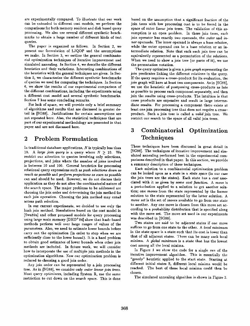
In Figure 1 we show the code for a single run of the iterative improvement algorithm. This is essentially the “greedy” heuristic applied to the start state. Starting at different initial states S, different local minima would be reached. The best of these local minima could then be chosen.

The simulated annealing algorithm is shown in Figure 2.

368

/* Get an initial solution */ S = initialize(); repeat {

/* Randomly select adjacent state */ news = move(S); if (cost(newS) < cost(S))

S = news; } until (“local minimum reached”);

Figure 1: One Run of Iterative Improvement

The determination of the parameter sizeFactor, the proce-

/* Get an initial solution */ S = initialize(); /* Set the initial temperature */ T = initialTempO; /* Set the chain length */ chainLength = sizeFactor * N; 1 = 0;

repeat { repeat {

1=1+1; /* Randomly select adjacent state */ news = move(S); delta = cost(newS) - cost(S); if (delta 5 0)

S = news; if (delta > 0)

S = news “with probability exp(-delta/T)“; } until (1 2 chainlength);

/* Reduce the temperature */ T = reduceTemp(T);

} until (“system has frozen”);

Figure 2: Simulated Annealing

dure reduceTemp, and the freezing condition are described in [SG88]. The stopping condition can include a maximum time limit. The optimizer can stop if it obtains a solution whose cost is sufficiently close to a lower bound on the cost of the optimal solution.

4 Heurist its A number of heuristics are commonly used in query optimization. It is expected that these heuristics are usually beneficial. For example, the heuristic push selections down as much as possible helps to decrease sizes of intermediate

results. The heuristic perform projections as soon as possible has a similar motivation. These two heuristics have been used by us to reduce the optimization problem to one of determining a good join order. The heuristic postpone cross-products as late as possible is very effective in prun- ing the search space to be searched. However, the space to be searched, namely, the valid space, is still too large for the queries we consider.

We will discuss three heuristics in this section. One heuristic, denoted as the KBZ heuristic, is the only heuristic known to us which was specifically proposed for optimizing nonrecursive large join queries [KBZSS]. Based on ideas of incrementally building good plans, we developed the augmentation heuristic described in 4.1. The algorithmic prin- ciple of “divide and conquer” gave rise to the third heuristic known as local improvement. While the KBZ and the augmentation heuristics directly generate a finite number of solutions, local improvement takes an existing solution as input, and seeks to improve it by a sequence of small transformations.

4.1 Augmentation Heuristic The augmentation heuristic builds a join tree (or the equiv- alent permutation) as follows. The first relation is picked according to some criterion. For instance, we may pick the smallest relation first. Corresponding to each choice of the first relation, the heuristic generates one permutation. Thus upto (N + 1) permutations can be generated corresponding to the (N + 1) joining relations. If all or some of these permutations are to be generated, the relations could be picked for the first position in order of increasing size.

Let S denote the set of relations that have already been placed in the permutation being generated. Let T denote the set of relations from which the next relation in the ordering is to be selected. Initially, S consists of the first relation, picked as indicated above. Then, the augmentation heuristic generates the rest of the permutation as shown in Figure 3.

perm[O] = first-relation; S = { first-relation }; T = { remaining relations };

for (i = 1; i < (N + 1); i = i + 1) { nextReln = chooseNext(S, T); perm[i] = nextReln; S = S + { nextReln }; T = T - { nextReln };

3

Figure 3: Augmentation Heuristic

The function chooseNext is passed the two sets S and T as input parameters, and returns a relation chosen from T according to some criterion. This criterion depends on the

369

relations in S. Note that only relations in T that join with at least one relation in S are considered. This ensures that only valid join trees are generated. Five different criteria were investigated. These are described below.

Let Nk denote the cardinality of relation k (this is the cardinality after all applicable selections have been performed). Let Dk denote the number of distinct values in the join column of relation k. Let deg(k) denote the number of relations that relation k joins with in the join graph. Let Jkr denote the join selectivity of the join of relations k and 1. Let i iterate over all the relations in S, and let j iterate over all the relations in T. Then the different criteria are:

1. min(Nj) - the relation with the smallest cardinality is chosen

2. max(deg(j)) - the relation with the highest degree in the join graph is chosen

3. min(kj) - the relation with the smallest join selectivity for the next join is chosen

4. min( Ni Nj Jij) - the relation that results in the smallest size for the next intermediate result is chosen

5. min((NiNjJij - l)/(O.SNi(Nj/Dj))) - the relation with the smallest “rank” (see [KBZSS]) is chosen

The goal is to keep the sizes of the intermediate relations as small as possible. Each criterion seeks to do this in a different way. Joining relations with the smallest cardinality first is an obvious way to achieve the goal (criterion 1). The second criterion is more subtle. The relations with the smallest cardinality may not be immediately available due to the constraint of avoiding cross products. Criterion 2 seeks to alleviate this problem by bringing as many relations as possible into the set T.

Criterion 3 tries to take into account that the join selectivity may be much more crucial than the cardinalities of the two joining relations. Criterion 4 seeks to combine the effects of criteria 1 and 3. Finally, criteria 5 seeks to minimize a calculated quantity called the ‘rank’ rather than the size of the intermediate relation. The rank can be thought of as the increase in the intermediate result normalized by the cost of doing the join. By using the rank measure, relations which do not produce intermediate results at great cost are preferred. The context in which the definition of rank arises is given in [KBZSS].

We carried out experiments to determine which criteria in the chooseNext function gives the best results. The average scaled costs for different time limits (see Section 6.1) for each of the criteria are given in Table 1. It is clear that the third criterion, namely, choosing the relation so that the next join has the smallest join selectivity, is the best criterion. The intuition behind why this criterion works best is that it tends to maximize the number of distinct values in the intermediate results, thus helping keep intermediate result sizes small throughout the evaluation of the query. The more direct criterion of choosing the relation resulting in the smallest immediate intermediate result size fares poorly because it neglects the effect of the number of distinct values in determining later intermediate result sizes. We used the criterion of join selectivity in the other experiments with the augmentation heuristic.

Vezt Criteria Time choose!

1 2 3 4 5

Table 1: Comparison of Criteria in Augmentation

4.2 KBZ Heuristic The KBZ heuristic algorithm is described in detail in [KBZSS]. The algorithm has been evaluated for queries with upto 15 joins in [vi187]. It is best viewed as consisting of a 3-level hierarchy of algorithms. The algorithm lowest in the hierarchy (algorithm R) expects to be given a join graph which is a rooted tree. The root is taken to be the first relation in the join ordering. Algorithm R returns the optimal join ordering for the input rooted tree. The next algorithm in the hierarchy (algorithm T) takes as input a join graph which is a tree, and finds the optimal order by iterating over all roots. For each choice of root, algorithm T calls algorithm R. The highest level algorithm (algorithm G) accepts a join graph (which could be cyclic), chooses a spanning tree for this graph, and then calls algorithm T to find the optimal order for this tree.

If cross products are to be avoided, a rooted join tree im- poses a partial ordering on the relations in the different join orderings, that is, only some of the possible join orderings are acceptable. The root is the first relation in any ordering. The root of each subtree must join before its descendants. However, relations which appear in different subtrees can be merged into the linear join ordering in many different ways. Algorithm R merges the subtrees in such a way that the relations are ordered by increasing rank values.

For a definition of rank, see Section 4.1. The definition of rank obtained in [KBZSS] depends on the cost function satisfying the following property. The cost function should have the form nrg(nz), where ni is the size of the outer operand and ns is the size of the inner operand, and g is a function. Note that the sort merge join method does not have a cost function of this form.

The heuristic behind algorithm R is that those relations which have lower rank should be joined before relations which have higher ranks. This seeks to minimize the cost of each new join, since the rank can be viewed as measuring the increase in the intermediate result per unit differential cost of doing the join. The hope is that in this fashion the total cost of the join ordering can be minimized. The complexity of algorithm R is O(N log(N)).

Algorithm T can use algorithm R to produce an optimal order for each choice of root in its input join tree. Since there are N + 1 choices for the root, it appears that algorithm T is of complexity O(N’log(N)). However, the al-

370

gorithm can be improved by performing the iteration over all roots by moving to adjacent relations. It can be shown that, on changing the root to an adjacent relation in the join tree, most of the computation in determining the optimal order for the previous root can be reused. The details are given in [KBZSS] where they show that the improved algorithm has complexity O(N’).

To extend the algorithm to handle join graphs which may be cyclic, algorithm G is used. Algorithm G chooses a minimum cost spanning tree from the join graph, and then applies algorithm T to this spanning tree. In [KBZSS], the authors suggest using the join selectivities as the weights for the edges in determining the best spanning tree.

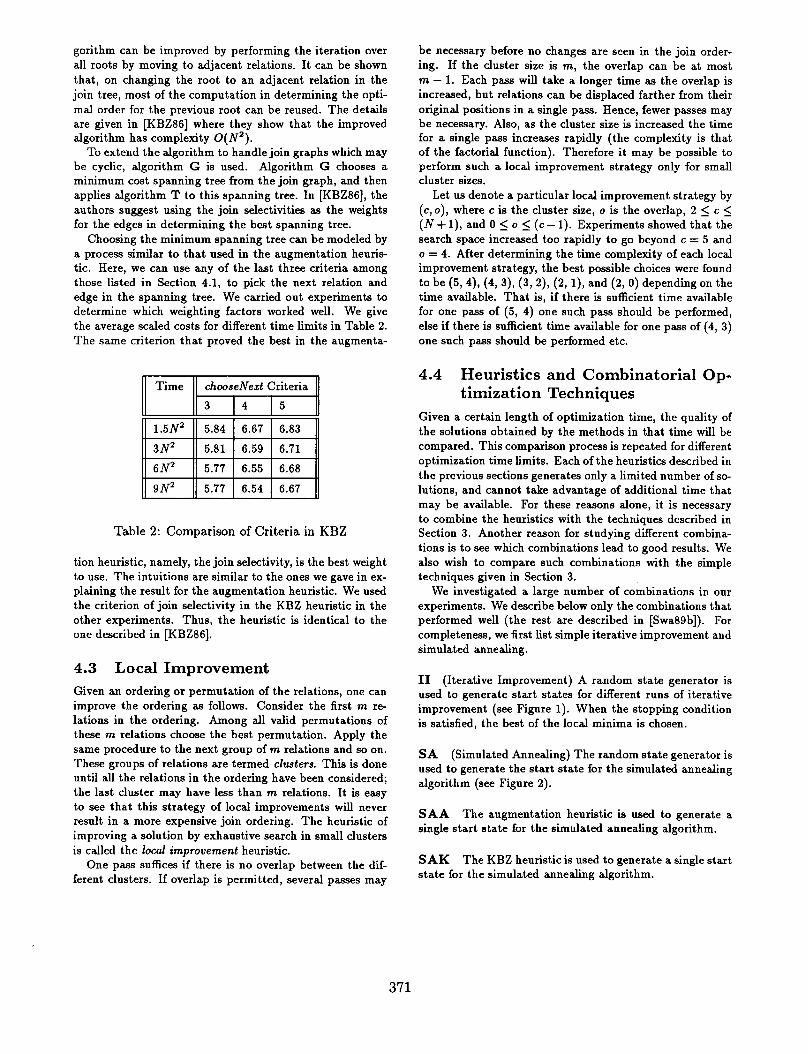
Choosing the minimum spanning tree can be modeled by a process similar to that used in the augmentation heuristic. Here, we can use any of the last three criteria among those listed in Section 4.1, to pick the next relation and edge in the spanning tree. We carried out experiments to determine which weighting factors worked well. We give the average scaled costs for different time limits in Table 2. The same criterion that proved the best in the augmenta-

9N2 5.77 6.54 6.67

Table 2: Comparison of Criteria in KBZ

tion heuristic, namely, the join selectivity, is the best weight to use. The intuitions are similar to the ones we gave in explaining the result for the augmentation heuristic. We used the criterion of join selectivity in the KBZ heuristic in the other experiments. Thus, the heuristic is identical to the one described in [KBZSS].

4.3 Local Improvement Given an ordering or permutation of the relations, one can improve the ordering as follows. Consider the first m relations in the ordering. Among all valid permutations of these m relations choose the best permutation. Apply the same procedure to the next group of m relations and so on. These groups of relations are termed clusters. This is done until all the relations in the ordering have been considered; the last cluster may have less than m relations. It is easy to see that this strategy of local improvements will never result in a more expensive join ordering. The heuristic of improving a solution by exhaustive search in small clusters is called the local improvement heuristic.

One pass suffices if there is no overlap between the different clusters. If overlap is permitted, several passes may

be necessary before no changes are seen in the join ordering. If the cluster size is m, the overlap can be at most m - 1. Each pass will take a longer time as the overlap is increased, but relations can be displaced farther from their original positions in a single pass. Hence, fewer passes may be necessary. Also, as the cluster size is increased the time for a single pass increases rapidly (the complexity is that of the factorial function). Therefore it may be possible to perform such a local improvement strategy only for small cluster sizes.

Let us denote a particular local improvement strategy by (c,o), where c is the cluster size, o is the overlap, 2 5 c 5 (N + l), and 0 5 o 5 (c - 1). Experiments showed that the search space increased too rapidly to go beyond c = 5 and o = 4. After determining the time complexity of each local improvement strategy, the best possible choices were found to be (5,4), (4, 3), (3,2), (2, l), and (2, 0) depending on the time available. That is, if there is sufficient time available for one pass of (5, 4) one such pass should be performed, else if there is sufficient time available for one pass of (4, 3) one such pass should be performed etc.

4.4 Heuristics and Combinatorial Op- timization Techniques

Given a certain length of optimization time, the quality of the solutions obtained by the methods in that time will be compared. This comparison process is repeated for different optimization time limits. Each of the heuristics described in the previous sections generates only a limited number of solutions, and cannot take advantage of additional time that may be available. For these reasons alone, it is necessary to combine the heuristics with the techniques described in Section 3. Another reason for studying different combinations is to see which combinations lead to good results. We also wish to compare such combinations with the simple techniques given in Section 3.

We investigated a large number of combinations in our experiments. We describe below only the combinations that performed well (the rest are described in [Swa89b]). For completeness, we first list simple iterative improvement and simulated annealing.

II (Iterative Improvement) A random state generator is used to generate start states for different runs of iterative improvement (see Figure 1). When the stopping condition is satisfied, the best of the local minima is chosen.

SA (Simulated Annealing) The random state generator is used to generate the start state for the simulated annealing algorithm (see Figure 2).

SAA The augmentation heuristic is used to generate a single start state for the simulated annealing algorithm.

SAK The KBZ heuristic is used to generate a single start state for the simulated annealing algorithm.

371

IA1 The augmentation heuristic generates the start states for different runs of iterative improvement. If all the states generated by the augmentation heuristic have been utilized and the stopping condition is not yet satisfied, the random state generator is used to generate start states for further runs of iterative improvement. When the stopping condition is satisfied, the best of the local minima is chosen.

IKI This combination is similar to IA1 except that the KBZ heuristic is used to provide the start states for the first set of iterative improvement runs.

IAL This combination is similar to IA1 except that after the states generated by the augmentation heuristic have been utilized, local improvement is applied to the best of the local minima obtained from the runs of iterative improvement.

AGI The augmentation heuristic is employed to generate different states. If the stopping condition is not yet satisfied, iterative improvement using the random state generator for obtaining start states is employed. When the stopping condition is satisfied, the best of the local minima and the states generated by the augmentation heuristic is chosen.

KBI This is similar to AGI except that the KBZ heuristic is used initially.

5 Evaluation Methodology To compare the different optimization techniques, we need to systematically generate a large number of queries. First, we specify distributions for various parameters of the queries. Generating random numbers according to these distributions, we obtain values for these parameters for a single query. Different queries are generated by specifying different initial seeds. In this way, we can obtain a large number of “random” queries.

N, the number of joins, is allowed to take values 10 through 100 (the number of joining relations is N + 1). The join graph is generated in two steps as follows. We first obtain a connected join graph using N joins so that the permutation (1 2 3 . . . N N + 1) is a valid permutation. Let S denote the set of relations that have already been linked. Initially, S consists of the relation 1. We iterate in numerical order over the relations 2 through N + 1; let the current relation to be linked be denoted by i. We pick a relation from S at random, link a’ with the chosen rela tion, and add i to S. In the second step, a parameter called the join cutoff probability is used. For each qualifying pair of relations, if a generated random number is less than the join cutoff probability, the two relations are linked by a join predicate.

The relation cardinality is the number of tuples in a relation. Each relation can have selection predicates that restrict the tuples of the relation that participate in joins with other relations. The number of distinct values in a

join column is an important factor in determining the size of intermediate results.

The features that characterize the queries generated are distributed as shown below. These distributions constitute the “default” distributions, and the benchmark synthesized using these distributions is the “default” benchmark. The motivations for choosing these distributions are explained in [SG88].

l Relation Cardinalities [lO,lOO) - 20%; [lOO,lOOO) - 60%; [lOOO,lOOOO) - 20%

0 Selections The number of selection predicates per relation ranges from 0 to 2. The selectivities of the selection predicates were chosen randomly from the following list:

0.001, 0.01, 0.1, 0.2, 0.34, 0.34, 0.34, 0.34, 0.34, 0.5, 0.5, 0.5, 0.67, 0.8, 1.0

l Distinct Values in join columns (as a fraction of the relation cardinality)

(0,0.2] - 90%; (0.2,1) - 9%; 1.0 - 1%

l Join Cutoff Probability = 0.01 In order to provide a more extensive comparison of the

different optimization methods, we varied the distributions so as to generate more extreme kinds of queries. These variations are divided into three classes. In the first class, we vary the distribution of the relation cardinalities. In the second class, we vary the distribution of the distinct values. Finally, we changed the manner in which the join graph was generated. In each class, three variations were used. When varying the distribution of one feature of the synthesized benchmark, the other distributions were kept the same (as in the default benchmark).

Relation Cardinalities The first variation is like the default distribution except that the range of the cardinalities is increased by a factor of 10. The increase in the range is of interest for two reasons. It can result in wider dispar- ities in relation sizes, potentially decreasing the number of good QEPs. Also, it results in more disk accesses in the disk based cost model.

In the second variation, the distribution is replaced by a uniform distribution over the range of cardinalities. This serves to model situations where nothing is known about the distribution of the relation cardinalities. The third variation is a combination of the first two variations. As in the first variation, the range is increased by a factor of 10, and, as in the second variation, a uniform distribution is used over the range of cardinalities. l [10,103) - 20%; [103,104) - 60%; [104,105) - 20% l [10,104) - uniform distribution s [10,105) - uniform distribution

Distinct Values In the first variation, there are more join columns with a larger number of distinct values. This results in smaller intermediate results on the average and may increase the fraction of good QEPs. The second variation is like the default distribution except that the range at the low end is decreased resulting in lower number of distinct values on the average. This has the effect of increasing

372

the average size of intermediate results, and makes the job of the optimizer harder since fewer QEPs are likely to be good.

The third variation is like the first variation, except that the range at the low end is decreased as in the second variation. Though these variations appear similar, one should note that small changes in the number of distinct values can lead to large changes in result sizes. l (0,0.2] - 80%; (0.2,1) - 16%; 1.0 - 4% 0 (O,O.l] - 90%; (O.&l) - 9%; 1.0 - 1% l (O,O.l] - 80%; (O.l,l) - 16%; 1.0 - 4%

Join Graph In the first variation, the join cutoff probability is increased. This means that the queries have more join predicates. As a result the optimizer may have to de- vote more time in generating individual QEPs. In the second and third variations, we change the manner in which the initial spanning tree is generated, thus changing the space of QEPs by changing its size and the fraction of good QEPs. Also, the last two variations generate important kinds of queries which are good tests of query optimizers.

In the second variation, the generation of the join predicates is biased towards generating “star-like” join graphs. In these graphs, a few relations are joined to a large number of other relations. This increases the size of the search space. In the third variation, the generation of the join predicates is biased towards generating “chain-like” join graphs. In these graphs, all relations are joined to only a few other relations. This decreases the size of the search space. l No bias, Join Cutoff Probability = 0.1 s Bias towards star graphs, join cutoff probability = 0.01 l Bias towards chain graphs, join cutoff probability = 0.01

6 Experimental Results The different methods were coded in C, and the experiments were run on very lightly loaded HP 9000/350 workstations. The workstation is based on a 25 Mhz 68020 processor, and is approximately a 4 MIPS machine. Note that the optimizer simulations are completely CPU bound; memory requirements are negligible compared to the main memory of the workstations.

For most experiments, we used 50 different queries for each of N = 10,20,30,40,50, giving a total of 250 different queries. Each algorithm was run twice on each query (using different initial seeds), thus giving two repli-

cates per query which were then averaged. For some experiments, we used 50 different queries for each of N = 10,20,30,40,50,60,70,80,90,100, giving a total of 500 different queries. The entire set of experimental runs took about 5000 hours of CPU time.

The majority of the experiments were performed using the default benchmark and the main memory cost model described in [Swa89a]. In the experiments where we changed the synthesized benchmarks, the cost model was left unchanged. Finally, in one set of experiments, we changed

the cost model to a disk based cost model similar to the one described in [Bra84].

6.1 Comparison of Algorithms All the experiments described in this section were con- ducted using the default benchmark and the main memory cost model. Unless otherwise indicated the experiments use the benchmark of 250 queries over N = 10 to 50. The experiments were performed for different time limits. The time limits are proportional to N’. At 9N2, the time limit for N = 50 is 7.5 minutes. The costs of the solutions obtained for each query at a particular time limit were scaled by di- viding by the best solution costs obtained at the time limit of 9N2.

For each technique, we can obtain the mean of the scaled solution costs obtained by that technique. Then, to compare the different techniques, we can simply compare the means of the scaled solution costs. The problem with this is that the mean is not a very robust statistic. It can be easily distorted by a few extreme values. An important intuition in query optimization research is that beyond a certain threshold, the ezact scaled cost of the QEP is unim- portant. For example, if we regard a QEP as useless if it has a scaled cost of 10 or greater, we do not wish to distinguish between two QEPs, one having a cost of 10, and the other a cost of 100. However, we need some measure like the mean for comparing the different optimization methods.

To resolve this problem, we define the notion of an outlying value. An outlying value is a final solution cost (obtained by some technique) which is much higher than the best solution cost. Intuitively, a technique performs poorly on a particularly query if the solution cost obtained by the technique is an outlying value. In our experiments we define a solution cost to be an outlying value if it is at least 10 times the best solution cost.

All outlying values are coerced to have a value of 10. This agrees with our intuition that once a solution is considered poor, we are not much interested from a practical point of view in how poor it is. Also, by not including the outlying values directly in the computation of the mean, we ensure that they do not skew the mean too much. The scaled solution costs after suitable trimming were averaged over the 250 queries to obtain one data point for a single algorithm at a particular time limit.

In Figure 4, we present the results of our first set of experiments comparing the nine methods described in Section 4. Note that all the methods show very little improvement near the time limit of 9N2. This indicates that we are comparing the methods over a reasonably comprehensive range of time. We see that IA1 is superior to all the other methods over almost the entire range of time. For the time limits less than l.5N2, AGI and II appear to be better. Note that the combinations using simulated annealing are clearly inferior. In the remaining experiments, we decided to concentrate on the top five methods, namely, IAI, AGI, II, IAL, and KBI.

In Figure 5, we compare these five methods using the benchmark of 500 queries over N = 10 to 100. The or-

373

6

A

E 5 r

9” e

s 4 C a 1 e d 3

C 0

: s 2

1

6

A V

F 5

g” e

: 4 a 1

ii 3

C 0

f s 2

1

oIA1 +AGI sI1 oIAL uKB1 l IK1 *SAK aSAA @SA

F

* : ‘, ‘.

a. ‘..‘..

9 -.:

‘Z..

‘. :::;e.:

‘0..

::::+;

Q.

:::!(

“.._

--i/l

;Q.:;;; . . . 8s:. Q

‘. .,

2,:: . . .

3 .o

0.3 1.5 3 4.5 6 7.5 9

Time (N’)

Figure 4: All Methods

oIA1 +AGI sI1 oIAL uKB1 U

. . +.

0

2:: 'S....

i ; ;g : :

'O...:

"...._, "...:g::.,.

"".....,,,, "...., .-j-....

.,, .'..._ . . ".., '.O.....

".O.....

.‘..V,/,

. . . . . .._ :::::. . . . . . s .o ““.,.

0.3 1.5 3 6 9

Time (N’)

Figure 5: Larger Benchmark

dering among the methods is unchanged. Again, we note that AGI and II are better than IA1 for small time limits. This is of interest because for optimizing ad hoc queries or queries that will be run only a few times, it is worthwhile identifying methods which do well (comparatively) at small time limits (even if they are inferior at larger time limits).

Hence, we decided to study the region of time from 0.3N2 to around 1.5N2 in greater detail for the three methods IAI, AGI, and II. The results for the benchmark of 500 queries are shown in Figure 6. We see that AGI is the method of choice until about 1.8N2. After this time limit, IA1 is better. The intuition behind the better performance

5

A V e r

g” e

S

Ii 4 1

ii

C 0 S t 8

3

o IA1 + AGI s II 0

s ‘.

‘. ‘0

I I I I I I

0.3 0.6 0.9 1.2 1.5 1.8 2.1

Time (N’)

Figure 6: Small Time Limits

of AGI at smaller time limits is that it permits exploration of many more join orderings obtained using the augmentation heuristic. IA1 expends time on runs of iterative improvement, and is unable to consider as many join orderings from the augmentation heuristic. This also indicates that the augmentation heuristic generates fairly good join orderings.

6.2 Changing the Cost Model We replaced the main memory cost model with a disk based cost model, and compared the methods using the benchmark of 250 queries. From Figure 7, we see that there is no alteration in the ordering among the methods. AGI is preferable for small time limits and beyond about 1.5N2, IA1 should be used. This implies that the characteristics of

374

the query plan space have not changed significantly when the cost models are changed.

5

A V

f 4

g” e

S C a 3 1

i

C 0

f 2 S

1

o IA1 + AGI s II o IAL u KBI n

I I I I I I I

0.3 1.5 3 4.5 6 7.5 9

Time (N’)

Figure 7: Disk Cost Model

6.3 Changing the Benchmarks We then compared the methods using the nine different benchmarks described in Section 5. We show the results in Table 3. These experiments were carried out at the

7 1.02 1.10

8 1.23 1.44

9 1.33 1.56

AGI 1 KBI 1 II

2.50 2.65 2.83

Table 3: Changing the Benchmarks

time limit of 9N2. The benchmarks are numbered from 1 through 9 in the order they appear in Section 5. The first three rows show the results for the benchmarks in which the distributions of the relation cardinalities were varied. The next three rows correspond to changing the distributions of the distinct values, and the last three rows depict the out- comes for the different ways in which the generation of the join graph was changed. We see that IA1 continues to be the method of choice irrespective of the benchmark used.

6.4 Discussion

In explaining these results, one should note that II was shown to be the best of the general combinatorial optimization techniques in [SG88]. We find that in the best combinations here, iterative improvement is used. Simulated annealing alone and the combinations involving simulated annealing are clearly inferior. One possible explanation of these results is that the solution space has a large number of local minima, with a small but significant fraction of them being deep local minima. Iterative improvement using the random state generator for generating the start states can traverse large regions of the search space and thus stands a good chance of finding one of the deep minima.

When aided by the augmentation heuristic, as in IAI, iterative improvement works even better. The heuristic provides (on the average) better starting points than the random state generator. For small time limits, it is likely that, in IAI, too much time is expended on reaching unprof- itable local minima. Hence, all the states which could be generated by the augmentation heuristic are not explored. Here AGI does better by first allowing for the generation of states by augmentation heuristic, and then employing iterative improvement.

The results regarding the KBZ heuristic are not encour- aging. It is a complex heuristic that takes much longer to generate a single state than the augmentation heuristic. This probably explains why the KBZ heuristic does so badly at small time limits. In comparison, the augmentation heuristic is trivial to implement. The local improvement heuristic also did not prove very useful. We only showed the results for IAL; the other methods in which local improvement was used were even less effective.

7 Summary The problem of optimizing large join queries is a hard combinatorial optimization problem. In a previous paper [SG88] we discussed the use of general combinatorial optimization techniques such as iterative improvement and simulated annealing to attack this problem. In this paper we study the use of heuristics to optimize large join queries, combining them profitably with iterative improvement and simulated annealing.

We discuss three heuristics, namely, augmentation, KBZ, and the local improvement heuristic. We experiment with a number of different combinations of these heuristics with the techniques of iterative improvement and simulated an-

375

nealing. We find that two combinations of iterative improvement and augmentation, namely, IA1 and AGI perform best. Of these, IA1 is the method of choice, except for small time limits when AGI is better. These results are unchanged when the main memory cost model was replaced by a disk based cost model. The ordering among the methods was also unaffected by the different synthetic benchmarks used.

Note that iterative improvement is one of the simplest combinatorial optimization techniques. The complex optimization technique of simulated annealing and its combinations do not fare well in the comparisons. Similarly, the augmentation heuristic is the simplest among the different heuristics discussed. Local improvement and the even more complex KBZ heuristic do not perform as well. These results lead us to speculate that until significant new insights are obtained into the characteristics of the search space, it will not be profitable to experiment with very complex methods for optimization.

Our work can be extended by incorporating join methods other than the hash join method. The distribution of solution costs in the space of valid solutions is of interest and is being investigated. Finally, the search for newer and improved heuristics usually never ends. We believe that our work provides a framework within which candidate heuristics can be compared with the methods we recommend in this paper.

Acknowledgements Prof. Gio Wiederhold, Prof. Anoop Gupta, and Jonathan Rose contributed to the work by way of stimulating discus- sions. The author thanks them, Peter Lyngbaek, Marie- Anne Neimat, and Waqar Hasan for providing useful com- ments on earlier drafts. The research is supported by Hewlett-Packard Laboratories under the contract titled “Research in Relational Database Management Systems” and, earlier, by DARPA contract N00039-84-C-0211 for Knowledge Based Management Systems.

References

[Bra841 K. Bratbergsengen. Hashing Methods and Rela- tional Algebra Operations. In Proceedings of the Tenth International Conference on Very Large Data Bases, pages 323-333, Singapore, Singa- pore, 1984. Morgan Kaufman.

[DKO+84] D. J. Dewitt, R. H. Katz, F. Olken, L. D. Shapiro, M. R. Stonebraker, and D. Wood. Implementation Techniques for Main Memory Database Systems. In Proceedings of ACM- SIGMOD International Conference on Manage- ment of Data, pages 1-8, June 1984.

[FBCt87] D. H. Fishman, D. Beech, H. P. Cate, E. C. Chow, T. Connors, J. W. Davis, N. Derrett, C. G. Hoch, W. Kent, P. Lyngbaek, B. Mahbod,

[IW87]

[JAMS871

[JK84]

[KBZSS]

[SAC+791

[SG88]

[Swa89a]

[Swa89b]

[vi1871

M. A. Neimat, T. A. Ryan, and M. C. Shan. Iris: An Object-Oriented DBMS. ACM Trans- actions on O&e Information Systems, 5(1):48- 69, January 1987.

Y. E. Ioannidis and E. Wong. Query Optimiza- tion by Simulated Annealing. In Proceedings of ACM-SIGMOD International Conference on Management of Data, pages 9-22, 1987.

D. S. Johnson, C. R. Aragon, L. A. McGeoch, and C. Schevon. Optimization by Simulated Annealing: An Experimental Evaluation (Part I). Draft, June 1987.

M. Jarke and J. Koch. Query Optimization in Database Systems. ACM Computing Surveys, 16(2):111-152, June 1984.

R. Krishnamurthy, H. Boral, and C. Zaniolo. Optimization of Nonrecursive Queries. In Pro- ceedings of the Twelfth International Confer- ence on Very Large Data Bases, pages 128-137, Kyoto, Japan, 1986. Morgan Kaufman.

P. Selinger, M. M. Astrahan, D. D. Chamber&r, R. A. Lorie, and T. G. Price. Access Path Selec- tion in a Relational Database Management Sy5 tern. In Proceedings of ACM-SIGMOD Inter- national Conference on Management of Data, 1979.

A. Swami and A. Gupta. Optimization of Large Join Queries. In Proceedings of ACM- SIGMOD International Conference on Manage- ment of Data, pages 8-17, 1988.

A. Swami. A Validated Cost Model For Main Memory Databases. To appear in Proceedings of ACM-SIGMETRICS Conference on Mea- surement and Modeling of Computer Systems, May 1989.

A. Swami. Optimization of Large Join Queries. PhD thesis, Stanford University, 1989. Draft in preparation.

E. E. Villarreal. Evaluation of an O(N*) Method for Database Query Optimization. Master’s thesis, The University of Texas at Austin, May 1987.

376

optimization of large join queries: combining heuristics and combinatorial techniques

Documents