optimal temperature−time programming in a batch copolymerization reactor

Optimal Temperature-Time Programming in a BatchCopolymerization Reactor

D. Salhi, M. Daroux, C. Gentric, J. P. Corriou, F. Pla, and M. A. Latifi*

Laboratoire des Sciences du Genie Chimique, CNRS-ENSIC, B.P. 451, 1 rue Grandville,54001 Nancy Cedex, France

This paper addresses the optimization of a batch copolymerization reactor of styrene andR-methylstyrene. The reactor is equipped with a jacket for heat exchange and, thus, fortemperature control. The performance index is the batch period, and the decision variable isthe jacket inlet temperature. The constraints involved include the process model, the polymerquality, the final monomer conversion rate, the heating/cooling rate of the reactor and upperand lower bounds of the variables. The optimization method is a direct method with a sequentialstrategy known as control vector parametrization method. The optimal profiles are determinedwith great care in terms of treatment and fulfilment of constraints. The results show a substantialimprovement with respect to the complete discretization method previously used.

1. Introduction

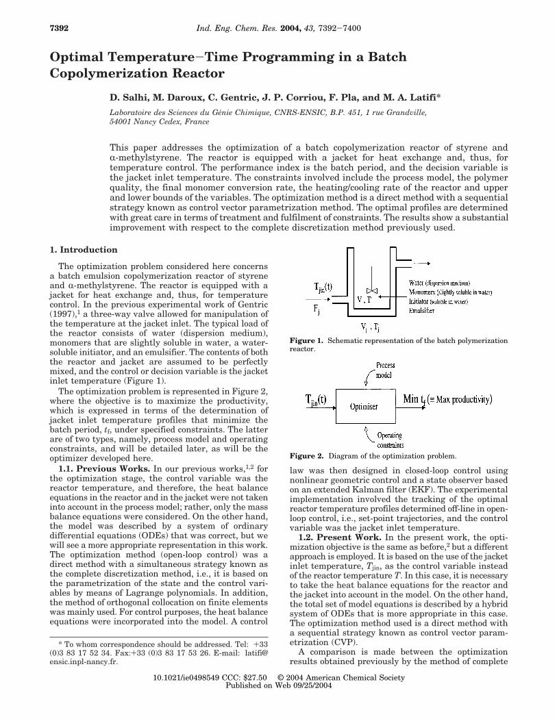
The optimization problem considered here concernsa batch emulsion copolymerization reactor of styreneand R-methylstyrene. The reactor is equipped with ajacket for heat exchange and, thus, for temperaturecontrol. In the previous experimental work of Gentric(1997),1 a three-way valve allowed for manipulation ofthe temperature at the jacket inlet. The typical load ofthe reactor consists of water (dispersion medium),monomers that are slightly soluble in water, a water-soluble initiator, and an emulsifier. The contents of boththe reactor and jacket are assumed to be perfectlymixed, and the control or decision variable is the jacketinlet temperature (Figure 1).

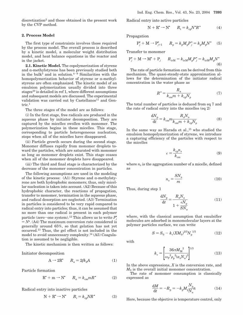
The optimization problem is represented in Figure 2,where the objective is to maximize the productivity,which is expressed in terms of the determination ofjacket inlet temperature profiles that minimize thebatch period, tf, under specified constraints. The latterare of two types, namely, process model and operatingconstraints, and will be detailed later, as will be theoptimizer developed here.

1.1. Previous Works. In our previous works,1,2 forthe optimization stage, the control variable was thereactor temperature, and therefore, the heat balanceequations in the reactor and in the jacket were not takeninto account in the process model; rather, only the massbalance equations were considered. On the other hand,the model was described by a system of ordinarydifferential equations (ODEs) that was correct, but wewill see a more appropriate representation in this work.The optimization method (open-loop control) was adirect method with a simultaneous strategy known asthe complete discretization method, i.e., it is based onthe parametrization of the state and the control vari-ables by means of Lagrange polynomials. In addition,the method of orthogonal collocation on finite elementswas mainly used. For control purposes, the heat balanceequations were incorporated into the model. A control

law was then designed in closed-loop control usingnonlinear geometric control and a state observer basedon an extended Kalman filter (EKF). The experimentalimplementation involved the tracking of the optimalreactor temperature profiles determined off-line in open-loop control, i.e., set-point trajectories, and the controlvariable was the jacket inlet temperature.

1.2. Present Work. In the present work, the opti-mization objective is the same as before,2 but a differentapproach is employed. It is based on the use of the jacketinlet temperature, Tjin, as the control variable insteadof the reactor temperature T. In this case, it is necessaryto take the heat balance equations for the reactor andthe jacket into account in the model. On the other hand,the total set of model equations is described by a hybridsystem of ODEs that is more appropriate in this case.The optimization method used is a direct method witha sequential strategy known as control vector param-etrization (CVP).

A comparison is made between the optimizationresults obtained previously by the method of complete

* To whom correspondence should be addressed. Tel: +33(0)3 83 17 52 34. Fax:+33 (0)3 83 17 53 26. E-mail: [email protected].

Figure 1. Schematic representation of the batch polymerizationreactor.

Figure 2. Diagram of the optimization problem.

7392 Ind. Eng. Chem. Res. 2004, 43, 7392-7400

10.1021/ie0498549 CCC: $27.50 © 2004 American Chemical SocietyPublished on Web 09/25/2004

discretization2 and those obtained in the present workby the CVP method.

2. Process Model

The first type of constraints involves those requiredby the process model. The overall process is describedby a kinetic model, a molecular weight distributionmodel, and heat balance equations in the reactor andin the jacket.

2.1. Kinetic Model. The copolymerization of styreneand R-methylstyrene has been previously studied bothin the bulk3 and in solution.4-9 Similarities with thehomopolymerization behavior of styrene or R-methyl-styrene are often emphasized. The kinetic model of anemulsion polymerization usually divided into threestages10 is detailed in ref 1, where different assumptionsand subsequent models are discussed. The experimentalvalidation was carried out by Castellanos11 and Gen-tric.1

The three stages of the model are as follows:(i) In the first stage, free radicals are produced in the

aqueous phase by initiator decomposition. They arecaptured by the micelles swollen with monomer. Thepolymerization begins in these micelles. This stage,corresponding to particle heterogeneous nucleation,stops when all of the micelles have disappeared.

(ii) Particle growth occurs during the second stage.Monomer diffuses rapidly from monomer droplets to-ward the particles, which are saturated with monomeras long as monomer droplets exist. This stage ceaseswhen all of the monomer droplets have disappeared.

(iii) The third and final stage is characterized by thedecrease of the monomer concentration in particles.

The following assumptions are used in the modelingof the kinetic process: (A1) Styrene and R-methylsty-rene are both hydrophobic monomers; thus, only micel-lar nucleation is taken into account. (A2) Because of thishydrophobic character, the reactions of propagation,transfer to monomer, termination in the aqueous phase,and radical desorption are neglected. (A3) Terminationin particles is considered to be very rapid compared toradical entry into particles; thus, it can be assumed thatno more than one radical is present in each polymerparticle (zero-one system).12 This allows us to write Pj

•

) N•. (A4) The maximum conversion rate considered isgenerally around 65%, so that gelation has not yetoccurred.13 Thus, the gel effect is not included in themodel to avoid unnecessary complexity.14 (A5) Coagula-tion is assumed to be negligible.

The kinetic mechanism is then written as follows:

The rate of particle formation can be derived from thismechanism. The quasi-steady-state approximation al-lows for the determination of the initiator radicalconcentration in the water phase as

The total number of particles is deduced from eq 7 andthe rate of radical entry into the micelles (eq 2)

In the same way as Harada et al.,15 who studied theemulsion homopolymerization of styrene, we introducea capturing efficiency of the particles with respect tothe micelles

where ns is the aggregation number of a micelle, definedas

Thus, during step 1

where, with the classical assumption that emulsifiermolecules are adsorbed in monomolecular layers at thepolymer particles surface, we can write

with

In the above expressions, X is the conversion rate, andM0 is the overall initial monomer concentration.

The rate of monomer consumption is classicallyexpressed as

Here, because the objective is temperature control, only

Initiator decomposition

A f 2R• Ra ) 2fkdA (1)

Particle formation

R• + m f N• Rn ) kcmmR • (2)

Radical entry into inactive particles

N + R• f N• Ri ) kcpNR • (3)

Radical entry into active particles

N + R• f N• Rt ) kcpN•R • (4)

Propagation

Pj• + M f Pj+1

• Rp ) kpMpP j• ) kpMpN

• (5)

Transfer to monomer

Pj• + M f M• + Pj RtrM ) ktrMMpP j

• ) ktrMMpN•

(6)

R • )Ra

kcmm + kcpNp(7)

dNp

dt) kcmm

RaNa

kcmm + kcpNp(8)

ε )kcpns

kcm(9)

ns )SNa

m(10)

dNp

dt)

RaNa

1 +εNp

SNa

(11)

S ) S0 - kv(XM0)2/3Np

1/3 (12)

kv ) [ 36πMM2

ωP2Fp

2(asNa)3]1/3

(13)

dMdt

) -Rp ) -kpMp

Np

Nanj (14)

Ind. Eng. Chem. Res., Vol. 43, No. 23, 2004 7393

the overall monomer concentration is described. Cas-tellanos11 studied the copolymerization of styrene andR-methylstyrene at three temperatures (50, 65, and 85°C) and four different initial monomer compositions (10,25, 35, and 50% by mass of R-methylstyrene). He foundexperimentally that no composition change occurredduring the polymerization under these conditions andshowed that the global propagation constant could bewritten as

where kpsty is the styrene homopolymerization propaga-tion rate constant, a is a constant, and fMS is the initialR-methylstyrene mole fraction.

The monomer concentration in the particles, Mp,corresponds to the particle saturation during steps 1 and2 and then decreases with increasing conversion rateduring step 3

Rudin and Samanta7 showed experimentally that nj isequal to 0.5 for styrene/R-methylstyrene copolymeriza-tion. Castellanos11 confirmed this value, even at highconversion rates.

2.2. Molecular Weight Distribution Model. Here,the molecular weight distribution model is based on thetendency model developed by Villermaux and Blavier.16

It consists of three ODEs where the unknowns are thedifferent moments of the molecular weight distribution.The integration of these equations leads to the number-and weight-average molecular weights and the polydis-persity index given by

where

and

The integration of these ordinary differential equations

(ODEs) provides the number- and weight-average mo-lecular weights and the polydispersity index

Remark. The rate constant for transfer to monomeris computed similarly to the propagation rate constant.Because no composition change occurs during thiscopolymerization under the conditions considered, aglobal constant is thus assumed.

2.3. Heat Balance Equations. Finally, the heatbalance equations in the reactor and in the jacket, thecontents of which are assumed to be perfectly mixed,are given, respectively, as

The initial temperatures can be considered as knownand equal to room temperature or as unknown param-eters to be optimized. Here, they are included in theoptimization process as unknown parameters.

2.4. Hybrid Representation of the Process Model.The resulting model is then a hybrid system of ODEswith two state modes denoted as 1 and 217

(i) Each mode is characterized by state and controlvariables, parameters, a set of ODEs, and a timeinterval in which these equations are defined.

Note that the upper bound of the time interval ofmode 2 is the batch period tf ) tf

(2). Note also that apossible discontinuity in control is taken into accountin these equations.

(ii) The switching time from mode 1 to mode 2 isdetermined by a transition condition

which, in our case, is the time when the monomerconversion rate equals its critical value (see eqs 16 and17).

(iii) The variables of the two modes at the transitiontime are linked through the following transition function

(iv) A special case of this transition condition is theset of initial conditions of the initial mode, which ismode 1

3. Operating Constraints

The second type of constraints is the operatingconstraints. They consist of (i) the lower and upper

kp ) kpsty exp(afMS) (15)

Mp ) Mpc )(1 - Xc)FM

[(1 - Xc) + XcFM/FP]MM

X e Xc, steps 1 and 2 (16)

Mp )(1 - X)FM

[(1 - X) + XFM/FP]MMX > Xc, step 3

(17)

dPdt

)dQ0

dt) Rt + RtrM

dQ1

dt) L(Rt + RtrM) ) Rp (18)

dQ2

dt) 2L2(Rt + RtrM)

Rt )RanjNp

Np + Sε

(19)

RtrM ) ktrMMp

Np

Nanj (20)

L )Rp

Rt + RtrM(21)

Mh n ) MM

Q1

Q0

Mh w ) MM

Q2

Q1(22)

Ip )Mh w

Mh n

dTdt

) - V∆HmrCp

Rp + UAmrCp

(Tj - T) (23)

dTj

dt)

Fj

Vj(Tjin - Tj) - UA

FjVjCj(Tj - T) (24)

mode 1 x3 (1) ) f(1)(x(1),u(1),p) t ∈ [t0(1), tf

(1)] (25)

mode 2 x3 (2) ) f(2)(x(2),u(2),p) t ∈ [t0(2), tf

(2)]

L(1)(x(1),u(1),p) ) 0 w t0(2) ) tf

(1) (26)

T(1)(x(1),u(1),x(2),u(2),p) ) 0 w x(2)(t0(2)) ) x(1)(tf

(1)) (27)

T0(1)(x(1), x0

(1)) ) 0 w x(1)(t0(1)) ) x0

(1) (28)

7394 Ind. Eng. Chem. Res., Vol. 43, No. 23, 2004

bounds of the seven state variables, the single controlvariable, and the two parameters

(ii) the final monomer conversion rate

(iii) the polymer quality expressed in terms of thenumber- or weight-average molecular weight

and (iv) finally the heating/cooling rate of the reactor

Note that the final conversion rate and polymer qualityconstraints are terminal-point equality constraints,whereas the heating/cooling rate is an infinite-dimen-sional inequality constraint.

The resulting optimization problem is then given by

subject to constraints 25-32.

4. Optimization Method

The above dynamic optimization problem involves theperformance index, which has to be optimized; theprocess model equations combined with initial stateconditions; and different types of constraints. Withoutloss of generality, a typical formulation of a dynamicoptimization problem can be stated as

subject to

The other types of constraints to be taken into accounttypically include infinite-dimensional, interior-point andterminal-point equality and inequality constraints.18,19

Moreover, they can be written in the following canonical

form similar to the cost form (eq 34)

where ti e tf, i ) 1, 2, ..., Nc, and Nc is the number ofconstraints.

For example, if an infinite-dimensional inequalityconstraint φ(x,u,p,t) e 0 is involved, then Gi ) 0 and Fi) ω(max{φ(x,u,p,t), 0]}2, where ω is an adjustableweight. The constraint is then expressed as Ji e 0. Inthe case of a terminal-point equality constraint φ-(x,u,p,tf) ) 0, Gi ) ω[φ(x,u,p,tf)]2 and Fi ) 0. Theconstraint is then expressed as Ji ) 0. The derivationof Gi and Fi for the other types of constraints isstraightforward.18

5. Optimality Conditions

5.1. Treatment of Constraints. To transform theconstrained optimization problem (eqs 34-36) into aproblem constrained only by the process model eqs 35,the following variables are defined

where νi represents the multipliers that are determinedat the optimum.

The resulting global performance index is given by

5.2. Optimality Conditions. For the resulting dy-namic optimization problem, eqs 40 and 35, the first-order necessary conditions for an optimum can bederived using the calculus of variations.20,21 It consistsof forming an augmented performance index Jh byappending the ODE constraints (eqs 35) to the cost (eq40) using the adjoint variables λ(t), defined by

The development of variations of the augmentedperformance index is straightforward. By setting δJhequal to zero, the first-order necessary conditions canbe derived as

with

xiL e xi(t) e xi

U, i ) 1, ..., 7

xT ) [M, Np, Q0, Q1, Q2, T, Tj]

uL e u(t) e uU, u ) Tjin

piL e pi(t) e pi

U, i ) 1, 2

pT ) [T0, Tj0] (29)

X(tf(2)) ) 1 -

x1(2)(tf

(2))

x10(1)

) Xf (30)

MM

x4(2)(tf

(2))

x3(2)(tf

(2))) Mh nf

or (31)

MM

x5(2)(tf

(2))

x4(2)(tf

(2))) Mh wf

|dTdt | ) |dx6

dt | e hcr (32)

minu(t),p

{J ) tf} (33)

minu(t),p

J0 ) G0[x(tf),p] + ∫t0

tfF0(x,u,p,t) dt (34)

x3 (t) ) f(x(t),u(t),p,t) with x(0) ) x0(p) (35)

Ji ) Gi[x(tf),p] + ∫t0

tiFi(x,u,p,t) dt (36)

J ) J0 + ∑i)1

i)Nc

νiJi (37)

G ) G0 + ∑i)1

i)Nc

νiGi (38)

F ) F0 + ∑i)1

i)Nc

νiFi (39)

minu(t),p

J ) G[x(tf),p] + ∫t0

tf F(x,u,p,t) dt (40)

λ(t) ) λ0(t) + ∑i)1

i)Nc

νiλi(t) (41)

x3 (t) )∂H∂λ

(42)

x(0) ) x0(p) (43)

λ4 (t) ) - ∂H∂x

(44)


with

where

Conditions 44, referred to as adjoint or costate equa-tions, allow for the determination of the profiles ofadjoint or costate variables λ(t). The correspondingboundary conditions are provided by conditions 45. Itis important to notice that the set of conditions (eqs 42-46) constitutes a two-point boundary value problem(TPBVP) because initial conditions 43 are specified forthe state equations (eq 42), whereas for costate eq 44,only terminal conditions 45 are available. BecauseTPBVPs are known to be very difficult to solve numeri-cally, appropriate computational methods are thereforeneeded.

6. Computational Methods

The numerical methods used for the solution ofdynamic optimization problems can be grouped into twocategories: indirect and direct methods.

6.1. Indirect Methods. The objective of indirectmethods is to solve the TPBVP (eqs 42-46), thusindirectly solving the dynamic optimization problemdefined by eqs 40 and 35. The most well-known methodsin this category are boundary condition iteration (BCI)and control vector iteration (CVI).22 However, thesemethods can exhibit numerical instabilities or slowconvergence rates for many problems.

6.2. Direct Methods. In this category, there are twostrategies: sequential and simultaneous. The sequentialstrategy, often called control vector parametrization(CVP), consists of approximating the control trajectoryby a function of only a few parameters and leaving thestate equations in the form of the original ODE sys-tem.18 Mostly, piecewise-constant control profiles areused. Hence, an infinite-dimensional optimization prob-lem in continuous control variables is transformed intoa finite-dimensional nonlinear programming (NLP)problem that can be solved by any gradient-basedmethod [e.g., a sequential quadratic programming (SQP)method23]. The performance index evaluation is carriedout by solving an initial value problem (IVP) of theoriginal ODE system, and gradients of the performanceindex as well as the constraints with respect to theparameters (p and approximations of u) can be evalu-ated by solving either the adjoint equations (eqs 44 and45)18 or the sensitivity equations.24 Moreover, thismethod is a feasible-type method, i.e., the solution isimproved at each iteration.

In the simultaneous strategy, both the control andstate variables are discretized using polynomials (e.g.,Lagrange polynomials) whose coefficients become thedecision variables in a much larger NLP problem.25,26

Unlike the CVP method, the simultaneous method doesnot require the solution of IVPs at every iteration of theNLP. The method is, however, of infeasible type, i.e.,the solution is available only once the iterative processhas converged.

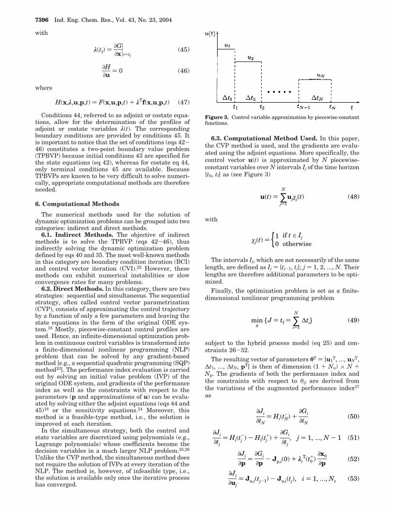
6.3. Computational Method Used. In this paper,the CVP method is used, and the gradients are evalu-ated using the adjoint equations. More specifically, thecontrol vector u(t) is approximated by N piecewise-constant variables over N intervals Ij of the time horizon[t0, tf] as (see Figure 3)

with

The intervals Ij, which are not necessarily of the samelength, are defined as Ij ) [tj-1, tj]; j ) 1, 2, ..., N. Theirlengths are therefore additional parameters to be opti-mized.

Finally, the optimization problem is set as a finite-dimensional nonlinear programming problem

subject to the hybrid process model (eq 25) and con-straints 26-32.

The resulting vector of parameters θT ) [u1T, ..., uN

T,∆t1, ..., ∆tN, pT] is then of dimension (1 + Nu) × N +Np. The gradients of both the performance index andthe constraints with respect to θij are derived fromthe variations of the augmented performance index27

as

λ(tf) ) ∂G∂x |t)tf

(45)

∂H∂u

) 0 (46)

H(x,λ,u,p,t) ) F(x,u,p,t) + λTf(x,u,p,t) (47)

Figure 3. Control variable approximation by piecewise-constantfunctions.

u(t) ) ∑j)1

N

ujøj(t) (48)

øj(t) ) {1 if t ∈ Ij

0 otherwise

minθ

{J ) tf ) ∑i)1

N

∆ti} (49)

∂Ji

∂tN) Hi(tN

-) +∂Gi

∂tN(50)

∂Ji

∂tj) Hi(tj

-) - Hi(tj+) +

∂Gi

∂tj, j ) 1, ..., N - 1 (51)

∂Ji

∂p)

∂Gi

∂p- Jp,i(0) + λi

T(t0+)

∂x0

∂p(52)

∂Ji

∂uj) Ju,i(tj-1) - Ju,i(tj), i ) 1, ..., Nc (53)


where

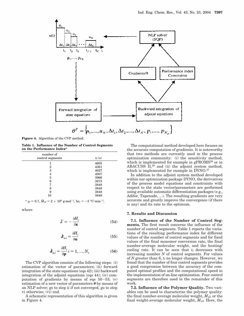
The CVP algorithm consists of the following steps: (i)estimation of the vector of parameters; (ii) forwardintegration of the state equations (eqs 42); (iii) backwardintegration of the adjoint equations (eqs 44); (iv) com-putation of gradients by means of eqs 50-53; (v)estimation of a new vector of parameters θ by means ofan NLP solver; go to step ii if not converged, go to stepvi otherwise; (vi) end.

A schematic representation of this algorithm is givenin Figure 4.

The computational method developed here focuses onthe accurate computation of gradients. It is noteworthythat two methods are currently used in the processoptimization community: (i) the sensitivity method,which is implemented for example in gPROMS28 or inABACUSS II,29 and (ii) the adjoint system method,which is implemented for example in DYNO.27

In addition to the adjoint system method developedwithin our optimization package DYNO, the derivativesof the process model equations and constraints withrespect to the state vector/parameters are performedusing available automatic differentiation packages (e.g.,Adifor, Tapenade, ...). The resulting gradients are veryaccurate and greatly improve the convergence (if thereis any) and its rate to the optimum.

7. Results and Discussion

7.1. Influence of the Number of Control Seg-ments. The first result concerns the influence of thenumber of control segments. Table 1 reports the varia-tions of the resulting performance index for differentvalues of the number of control segments and for fixedvalues of the final monomer conversion rate, the finalnumber-average molecular weight, and the heating/cooling rate. It can be seen that tf decreases withincreasing number N of control segments. For valuesof N greater than 6, tf no longer changes. However, wefound that the number of four control segments providesa good compromise between the accuracy of the com-puted optimal profiles and the computational speed inthe implementation of on-line optimization. Four controlsegments are therefore used in the remainder of thiswork.

7.2. Influence of the Polymer Quality. Two vari-ables can be used to characterize the polymer quality:the final number-average molecular weight, Mh nf, or thefinal weight-average molecular weight, Mh wf. Here, the

Figure 4. Algorithm of the CVP method.

Table 1. Influence of the Number of Control Segmentson the Performance Indexa

number ofcontrol segments tf (s)

1 46052 43613 40274 40075 39666 38737 38488 38489 3848

10 3848a øf ) 0.7, Mh nf ) 2 × 106 g‚mol-1, hcr ) -3 °C‚min-1.

λ4 i ) -∂Hi

∂x(54)

J4 u,i )∂Hi

∂u(55)

J4 p,i )∂Hi

∂pi ) 1, ..., Nc (56)


influence of Mh nf is analyzed. The influence of Mh wf doesnot pose any specific problem and is not investigatedhere only for brevity.

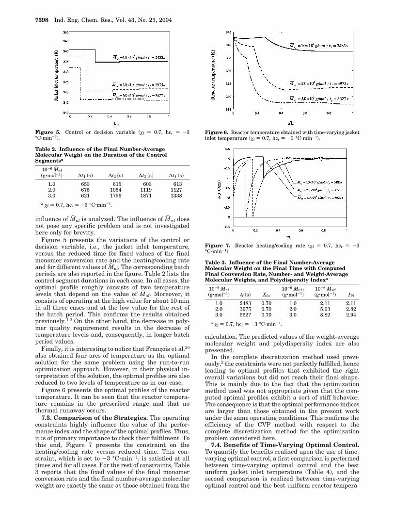
Figure 5 presents the variations of the control ordecision variable, i.e., the jacket inlet temperature,versus the reduced time for fixed values of the finalmonomer conversion rate and the heating/cooling rateand for different values of Mh nf. The corresponding batchperiods are also reported in the figure. Table 2 lists thecontrol segment durations in each case. In all cases, theoptimal profile roughly consists of two temperaturelevels that depend on the value of Mh nf. Moreover, itconsists of operating at the high value for about 10 minin all three cases and at the low value for the rest ofthe batch period. This confirms the results obtainedpreviously.1,2 On the other hand, the decrease in poly-mer quality requirement results in the decrease oftemperature levels and, consequently, in longer batchperiod values.

Finally, it is interesting to notice that Francois et al.30

also obtained four arcs of temperature as the optimalsolution for the same problem using the run-to-runoptimization approach. However, in their physical in-terpretation of the solution, the optimal profiles are alsoreduced to two levels of temperature as in our case.

Figure 6 presents the optimal profiles of the reactortemperature. It can be seen that the reactor tempera-ture remains in the prescribed range and that nothermal runaway occurs.

7.3. Comparison of the Strategies. The operatingconstraints highly influence the value of the perfor-mance index and the shape of the optimal profiles. Thus,it is of primary importance to check their fulfilment. Tothis end, Figure 7 presents the constraint on theheating/cooling rate versus reduced time. This con-straint, which is set to -3 °C‚min-1, is satisfied at alltimes and for all cases. For the rest of constraints, Table3 reports that the fixed values of the final monomerconversion rate and the final number-average molecularweight are exactly the same as those obtained from the

calculation. The predicted values of the weight-averagemolecular weight and polydispersity index are alsopresented.

In the complete discretization method used previ-ously,2 the constraints were not perfectly fulfilled, henceleading to optimal profiles that exhibited the rightoverall variations but did not reach their final shape.This is mainly due to the fact that the optimizationmethod used was not appropriate given that the com-puted optimal profiles exhibit a sort of stiff behavior.The consequence is that the optimal performance indicesare larger than those obtained in the present workunder the same operating conditions. This confirms theefficiency of the CVP method with respect to thecomplete discretization method for the optimizationproblem considered here.

7.4. Benefits of Time-Varying Optimal Control.To quantify the benefits realized upon the use of time-varying optimal control, a first comparison is performedbetween time-varying optimal control and the bestuniform jacket inlet temperature (Table 4), and thesecond comparison is realized between time-varyingoptimal control and the best uniform reactor tempera-

Figure 5. Control or decision variable (øf ) 0.7, hcr ) -3°C‚min-1).

Table 2. Influence of the Final Number-AverageMolecular Weight on the Duration of the ControlSegmentsa

10-6 Mh nf(g‚mol-1) ∆t1 (s) ∆t2 (s) ∆t3 (s) ∆t4 (s)

1.0 653 615 603 6132.0 675 1054 1119 11273.0 621 1796 1871 1338

a øf ) 0.7, hcr ) -3 °C‚min-1.

Figure 6. Reactor temperature obtained with time-varying jacketinlet temperature (øf ) 0.7, hcr ) -3 °C‚min-1).

Figure 7. Reactor heating/cooling rate (øf ) 0.7, hcr ) -3°C‚min-1).

Table 3. Influence of the Final Number-AverageMolecular Weight on the Final Time with ComputedFinal Conversion Rate, Number- and Weight-AverageMolecular Weights, and Polydispersity Indexa

10-6 Mh nf(g‚mol-1) tf (s) Xf,c

10-6 Mh nf,c(g‚mol-1)

10-6 Mh wf(g‚mol-1) IPf

1.0 2483 0.70 1.0 2.11 2.112.0 3975 0.70 2.0 5.63 2.823.0 5627 0.70 3.0 8.82 2.94

a øf ) 0.7, hcr ) -3 °C‚min-1.


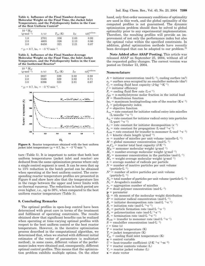
ture (Table 5). It is important to notice that both bestuniform temperatures (jacket inlet and reactor) arededuced from the same optimization process where onlya single control segment is used. It can be seen that upto 15% reduction in the batch period can be obtainedwhen operating at the best uniform control. The corre-sponding reactor temperature profiles are presented inFigure 8 and show here also that the temperature liesin the range between the upper and lower limits withno thermal runaway. The reductions in batch period areeven higher, i.e., up to 30%, when compared to the bestuniform reactor temperature (Table 5).

8. Concluding Remarks

The optimal profiles in open-loop control have beendetermined with great care in terms of the treatmentand fulfilment of operating constraints. The resultsobtained show that significant benefits can be realizedwhen operating at time-varying optimal profiles withrespect to the best uniform control or the best reactortemperature. However, in the iterative optimizationprocess described in the computational algorithm, wedetermined that, when we started with different initialestimates of the vector of parameters (a multistartmethod), in some cases, different values of the perfor-mance index were obtained and, consequently, differentoptimal control profiles. This means that the optimiza-tion problem exhibits multiple optima. On the other

hand, only first-order necessary conditions of optimalityare used in this work, and the global optimality of thecomputed profiles is not guaranteed. The dynamicoptimization problem should then be solved to globaloptimality prior to any experimental implementation.Therefore, the resulting profiles will provide an im-provement of not only the performance index but alsothe optimal value within the specified constraints. Inaddition, global optimization methods have recentlybeen developed that can be adapted to our problem.31

Note Added after ASAP Posting. This article wasreleased ASAP on September 25, 2004, without all ofthe requested galley changes. The correct version wasposted on October 13, 2004.

Nomenclature

A ) initiator concentration (mol‚L-1), cooling surface (m2)as ) surface area occupied by an emulsifier molecule (dm2)Cj ) cooling fluid heat capacity (J‚kg-1‚K-1)f ) initiator efficiencyFj ) cooling fluid flow rate (L‚s-1)fMS ) R-methylstyrene molar fraction in the initial loadH ) Hamiltonian functionhcr ) maximum heating/cooling rate of the reactor (K‚s-1)Ip ) polydispersity indexJ ) objective functionkcm ) rate constant for initiator radical entry into micelles

(L‚micelle-1‚s-1)kcp ) rate constant for initiator radical entry into particles

(L‚part-1‚s-1)kd ) rate constant for initiator decomposition (s-1)kp ) rate constant for propagation (L‚mol-1‚s-1)ktrM ) rate constant for transfer to monomer (L‚mol-1‚s-1)L ) kinetic chain length (g‚mol-1)m ) number of micelles per unit volume (micelle‚L-1)M ) global monomer concentration (mol‚L-1)mrCp ) reactor total heat capacity (J‚K-1)MM ) monomer molecular weight (g‚mol-1)Mh n ) number-average molecular weight (g‚mol-1)Mp ) monomer concentration in the particles (mol‚L-1)Mh w ) weight-average molecular weight (g‚mol-1)nj ) average number of radicals per particleN ) number of inactive particles per unit volume

(particle‚L-1)N • ) number of active particles per unit volume

(particle‚L-1)Np ) total number of particles per unit volume (particle‚L-1)Na ) Avogadro’s numberns ) aggregation number of micellesP ) dead polymer concentration (mol‚L-1)p ) parameterQi ) ith moment of the molecular weight distributionR • ) initiator radical concentration (mol‚L-1)Ra ) initiator decomposition rate (mol‚L-1‚s-1)Ri ) initiation rate (mol‚L-1‚s-1)Rn ) particle formation rate (mol‚L-1‚s-1)Rp ) polymerization rate (mol‚L-1‚s-1)Rt ) termination rate (mol‚L-1‚s-1)RtrM ) transfer to monomer rate (mol‚L-1‚s-1)S ) emulsifier concentration (mol‚L-1)t ) time (s)T ) reactor temperature (K)Tj ) jacket temperature (K)Tjin ) cooling fluid inlet temperature (K)u ) control variableU ) heat-transfer coefficient (J‚K-1‚s-1‚m-2)V ) reactor contents volume (L)Vj ) reactor jacket volume (L)x ) state vector

Table 4. Influence of the Final Number-AverageMolecular Weight on the Final Time, the Jacket InletTemperature, and the Polydispersity Index in the Caseof the Best Uniform Controla

10-6 Mh nf(g‚mol-1) tf (s) Tjin (K) IPf tf/tf

uniform

1.0 2701 336 2.03 0.922.0 4605 326 2.13 0.863.0 6450 321 2.21 0.87

a øf ) 0.7, hcr ) -3 °C‚min-1.

Table 5. Influence of the Final Number-AverageMolecular Weight on the Final Time, the Inlet JacketTemperature, and the Polydispersity Index in the Caseof the Isothermal Reactora

10-6 Mh nf(g‚mol-1) tf (s) Tjin (K) IPf tf/tf

isotherm

1.0 2827 339 2.02 0.882.0 5588 329 2.02 0.713.0 8396 323 2.01 0.67

a øf ) 0.7, hcr ) -3 °C‚min-1.

Figure 8. Reactor temperature obtained with the best uniformjacket inlet temperature (øf ) 0.7, hcr ) -3 °C‚min-1).


X ) conversion rateXc ) critical conversion rate

Greek Symbols

∆H ) polymerization reaction enthalpy (J‚mol-1)ε ) constant describing the efficiency of the particles

relative to the micelles in collecting an initiator radicalλ ) adjoint variableFp ) polymer particle density (g‚L-1)Fj ) cooling fluid density (g‚L-1)FM ) monomer density (g‚L-1)FP ) polymer density (g‚L-1)θ ) parameter vectorωP ) polymer weight fraction in the particles

Subscripts

f ) final0 ) initial

Literature Cited

(1) Gentric, C. Optimisation Dynamique et Commande nonLineaire d’un Reacteur de Polymerisation en Emulsion. Ph.D.Thesis, INPL, Nancy, France, 1997.

(2) Gentric, C.; Pla, F.; Latifi, M. A.; Corriou, J. P. Optimizationand nonlinear control of a batch emulsion polymerization reactor.Chem. Eng. J. 1999, 75, 31-46.

(3) O’Driscoll, K. F.; Dickson, J. R. Copolymerization withdepropagation. II. Rate of copolymerization of styrene-R-meth-ylstyrene. J. Macromol. Sci. A: Chem. 1968, 2, 449-457.

(4) Branston, R. E.; Plaumann, H. P.; Sendorek, J. J. Emulsioncopolymers of R-methylstyrene and styrene. J. Appl. Polym. Sci.1990, 40, 1149-1162.

(5) Johnston, H. K.; Rudin, A. Free radical copolymerizationof R-methylstyrene and styrene. J. Paint. Technol. 1970, 43, 435-448.

(6) Rudin, A.; Chiang, S. S. Kinetics of free-radical copolymer-ization of R-methylstyrene and styrene. J. Polym. Sci. A: Polym.Chem. 1974, 12, 2235-2254.

(7) Rudin, A.; Samanta, M. C. Emulsion copolymerization ofR-methylstyrene and styrene. J. Appl. Polym. Sci. 1979, 24, 1665-1689.

(8) Rudin, A.; Samanta, M. C. Emulsion copolymers of R-me-thylstyrene and styrene. J. Appl. Polym. Sci. 1979, 24, 1899-1916.

(9) Rudin, A.; Samanta, M. C.; Van der Hoff, B. M. E. Monomerchain-transfer constants from emulsion copolymerization data:Styrene and R-methylstyrene. J. Polym. Sci. A: Polym. Chem.1979, 17, 493-502.

(10) Smith, W. V.; Ewart, R. H. Kinetics of emulsion polymer-ization. J. Chem. Phys. 1948, 16, 592-599.

(11) Castellanos, J. R. Contribution a la modelisation duprocede de copolymerisation en emulsion de l′R-methylstyrene etdu styrene. Ph.D. Thesis, INPL, Nancy, France, 1996.

(12) Asua, J. M.; Adams, M. E.; Sudol, E. D. A new approachfor the estimation of kinetic parameters in emulsion polymeriza-tion systems. J. Appl. Polym. Sci. 1990, 39, 118-1213.

(13) Gerrens, H. Uber den Geleffekt bei der Emulsions Poly-merisation von Styrol. Z. Elektrochem. 1956, 60, 400-404.

(14) Qin, J.; Li, H.; Zhang, Z. Modeling of high-conversionbinary copolymerization. Polymer 2003, 44, 2599-2604.

(15) Harada, M.; Nomura, M.; Kojima, H.; Eguchi, W.; Nagata,S. Rate of emulsion polymerization of styrene. J. Appl. Polym. Sci.1972, 16, 811-833.

(16) Villermaux, J.; Blavier, L. Free radical polymerizationengineeringsI A new method for modeling free radical homoge-neous polymerization reactions. Chem. Eng. Sci. 1984, 39, 87-99.

(17) Galan, S.; Feehry, W. F.; Barton, P. I. Parametric sensitiv-ity function for hybrid discrete/continuous systems. Appl. Numer.Math. 1999, 31, 17-47.

(18) Goh, C. J.; Teo, K. L. Control parametrization: A unifiedapproach to optimal control problems with general constraints.Automatica 1988, 24, 3-18.

(19) Teo, K. L.; Goh, C. J.; Wong, K. H. A Unified Computa-tional Approach to Optimal Control Problems; John Wiley andSons: New York, 1991.

(20) Pontryagin, L. S.; Boltyanskii, V. G.; Gamkrelidze, R. V.;Mishchenko, E. F. The Mathematical Theory of Optimal Processes;Pergamon Press: New York, 1964.

(21) Bryson, A. E.; Ho, Y. C. Applied Optimal Control; Hemi-sphere Publishing Corporation: New York, 1975.

(22) Ray, W. H.; Szekely, J. Process Optimization with Applica-tions in Metallurgy and Chemical Engineering; John Wiley andSons: New York, 1973.

(23) Schittkowski, K. NLPQL: A FORTRAN subroutine solvingconstrained nonlinear programming problems. Ann. Oper. Res.1985, 5, 485-500.

(24) Feehery, W. F. Dynamic optimization with path con-straints. Ph.D. Thesis, MIT, Cambridge, MA, 1998.

(25) Biegler, L. T. Solution of dynamic optimization problemsby successive quadratic problems and orthogonal collocation.Comput. Chem. Eng. 1984, 8, 243-248.

(26) Cuthrell, J. E.; Biegler, L. T. On the optimization ofdifferential-algebraic process systems. AIChE J. 1987, 33, 1257-1270.

(27) Fikar, M.; Latifi, M. A. User’s Guide for FORTRANDynamic Optimisation Code DYNO; Technical Report: Laboratoiredes Sciences du Genie Chimique, CNRS: Nancy, France, 2002.

(28) Barton, P. I.; Pantelides, C. C. gPROMS: A combineddiscrete/continuous environment for chemical processing systems.Simul. Ser. 1993, 25, 25-34.

(29) Tolsma, J. E.; Clabaugh, J.; Barton, P. I. ABACUSS II:Advanced Modeling Environment and Embedded Simulator;MIT: Cambridge, MA, 1999 (see http://yoric.mit.edu/abacuss2/abacuss2.html).

(30) Francois, G.; Srinivasan, B.; Bonvin, D. Run-to-run opti-mization of batch emulsion polymerization. In Proceedings of theIFAC World Congress; Elsevier Science Ltd.: Amsterdam, 2002;pp 1258-1263.

(31) Chachuat, B.; Latifi, M. A. A new approach in deterministicglobal optimisation of problems with ordinary differential equa-tions. In Nonconvex Optimization and Its Applications; Floudas,C. A., Pardalos, P. M., Eds.; Kluwer Academic Publishers: Dor-drecht, The Netherlands, 2004; pp 83-108.

Received for review February 20, 2004Revised manuscript received September 8, 2004

Accepted September 13, 2004

IE0498549


optimal temperature−time programming in a batch copolymerization reactor

Documents