IEEE Transactions on Power Systems, Vol. 13, No. 3, August 1998

Optimal Smoothing for Trend Removal in Short Term Electricity Demand Forecasting

D. G. Infield CREST, Department of Electronic and Electrical Engineering,

Loughborough University Loughborough, Leiccstershire, LE 1 1 3TU, IJK

D. C. Hill School of Ocean Science

University Cclllege of Noi-th Wales Meiiai Bridge, Gwynedd, LL59 5EY, UK

Abstract-Changes to the electricity supplx industry, in particular the progress toma rcl s d creg ulat ion, t i :we prompted an increased interest in short term electricity demand forecasting. Trend removal has been identifiec!l as a key element in forecasting, and perhaps the area that can most benefit from the application of atlwnccd time series analysis. A new approach to trend removal is prcscntctl I)asctl on fixed intenal, or optimal, snioothing techniques. Forecasts clcriwxl in this way are compared with more con\.en tion al approaches. P reli iii i t i a ry res u Its i t i t l icate the new method to I)e promising and tlcscrving of further tle\.clopment.

Electricity demand foi-ccasting IS impoitant for the clecti-i'ity s u p p l j ~ industiy (131) for both long tcim planning, and for the implcnientation of iiiipro\d plant scheduling. With the stiuctiii-a1 changes to the ESI o\w recent years there IS an iiicrcascd emphasis on shot-t tcmm load rol-cc:lsting. 'l'his folio\\ s t o :I great extent from the economic value to pi-i\.arised: and inci-easii-lgly deregulatcd, sections of the 131 of lxing able to pixdiet shol-t teim fluctuations in electricity generation costs. With thc \\idci. a\dahiliT of computer based po~vei- 111 operational planr ing tools, i t is now feasiblc for smaller systems and suhsection.; of larger systems to benefit fi-om sophisticatcd load predictions

Conventional prediction methods are reviemed in Magd and Sinha [ l ] aiid the book by Bunn and Farmer [2]. A i-ec:ent adaptation of these tecliniques to shoit teim forecasting and its application to a nieso-scale island po\ver system ( peak load

PE-356-PWRS-1-09-1997 A paper recommended and approved by the IEEE Power System Engineering Committee of the IEEE Power Engineering Society for publication in the IEEE Transactions on Power Systems. Manuscript submitted July 26, 1996; made available for printing October 3, 1997.

1115

around 35 MW) has been undertaken by Hill and Infield, [ 3 ] . This study highlighted the importance of trend removal in the forecasting process.

Much of the recently published work on shoi-t term load forecasting has been concerned with the application of Artificial Neural Net\voi-ks (ANNs) and fuzzy logic, foi- example [4], [5] and [6] . Both of thcse approaches have been demonstrated to function well with particular data sets but do not coinmand the conlidencc of the Electi-icity Supply Industry (ESI) due to a lack of intuitive rclation to the processes which determine the electricity demand. Furtheimore, it has been identified that a key limitation of tlic ANN is its relative inability to adapt to reflect changing conditions, 151. This is of particular concern when applicd to clectricily demand forecasting since electricity supply

tetiis tend to expand significantly with time and theii- charactci-islics are continuousl)~ evolving. In contrast, it is bclieved that tlic techniques prcseiitcd here, being based fiiiiily on time scrics analysis and the f'amiliai- dccomposition ofthe load, \ \ r i l l hc attracti\re to thc f 5 1 : 1 tideed they \yere initially developed in closc collalwt-atton \ v i h a pal-ticular electi-icity supply coiiipany: tlic North of Scotland I-lydi-o Electi-ic Boai-d.

A ne\\. approach to trend rc:nio\.al has bcen developed based on optimal smoothing (sometimes referred to as fixed interval snicmtliing) One hour ahead load forccasts have been calculated for the Shetland mcso-scak tem, [3]: utilising existing high quality load data available from a previous study of the island system, 171.

11. DESCRIPTION OF FORECASTING METHODS

Conip:iiisoii IS made bet\veen the new load forecasting method and two conventional approaches. both of which use the 'standard day approach <or trcnd reino\:al. The diff'erence between the two conventional methods lies in the forecasting of the nominally stochastic (dctrcnded) load component. In the first technique a straightfoiward persistence forecast is used whilst the second approach makes use of a seasonal autoregressive (AR) model.

The ne\\' forecasting appiroaeh also applies AR modelling to the detrended data; its novelty consists in the approach to trend rcmoval.

0885-8950/9t;/$10.00 0 1997 IEEE

1116

In the 'standard day' methodology for electricih demand forecasting the load, L, is decomposed into components. Since comparison will be made with results obtained using the methods presented in [ 3 ] : this paper \vi11 follow the approach and nomenclahue adopted within that paper. The decomposilion used in the previous study was: i ) the annual component due to seasonal wcather pattenis, i i ) thc diuinal component due to daily behavioural pattein of the inhabitants, L,, and iii) the stochastic remainder, L, Each of these components is forecast sepal-ately and the results summated to pi-ovide the overall forecast. The annual component is modelled by the variation in weekly mean which is forecast using persistence (ie the predicted value for the weeklv mean is the mean for the preceding \\reek). In the notation of 131; LA,,(ii+1) = L,(ii9. \\here I V is the \\.e& number and "" denotes a forecast,

An average over n pi-esciihcd numhei- 01' ~veeks. I?,,,, p ~ o r to the cun-ent iwck is used to repi-escnt \hc diumal component:

W

for d = 1.2 ,... 7 , / I = I .2 24. \\.here d is the day nuimher. / I thc hour number. and whci-e the averaging starts at \\:eel; II:, = w - (n,,.-l). This axrage is calculated for each hour for each do!; of the \\reek so that the load pattem h i - h dny of the \\,eci\ is evaluated independently. This \I :IS found to bc important chic to the significant \,ariations hct\\'ccn ctays 01' thc \ \ w k

A radically diffei-ent appmacli to trend rcmoval has been de\~eloped based on optimal sinoothing. Pre\ious \ w r k identified the significant variation of load \vith both time and da!~ of' the week. It is suggested tha t tlie best guide to the load value for a particular hour of the day is tlie value of the load for the same hour and day of the pre\.ious \leek. 1.e. the hourly mean, 168 hours earlier. Variations i n this hourly load ~ d u c can he expected due to slo\v aniiual changes ivliich rellect changing temperature and houi-s of daylight. On this basis i t \vas decided to forecast the hourly mean fi-om a time series of \.slues i'or preceding weeks. Each hour of the \veek \vi11 he trciired separately resulting in 168 difhcnt time sei-ies bcing indi\.iduall!. forecast. The \\;eckl>. patteiii or trend used in the con\wtional decomposition, can be regained bv assembling tlic indi\kiu:il forecasts and the stochastic rcmaindcr is calculated in the same way as before.

Because tlie time series of these iveeklv t ~ ~ l u e s (for each hour) are found to be smoothly vai-ying a modelling and forecasting

approach based on optimal smoothing was selected. The method has the ciucial advantage over simpler forecasting

approaches such as exponential smoothing, of having no time delay (or phase effect). Such a delay would be unacceptable for forecasting of this trend since it involves data points one week apart.

A fonnulation of the optimal smoothing algorithm due to Ng and Young, [8], has been used in which the trend model is taken as an integrated random walk (IRW) and the degree of smoothing is controlled by a single parameter, known as the noise variance ratio (NVR). Note that the trend referred to here is that for a pai-ticular hour of the week, and must be distinguished from the weekly load pattein or trend discussed earlier. An NVR of zero results in a least squares linear trend, whilst, as the NVR increases, the trend increasingly follows the fluctuations in the original data. The NVR deteimines, as its name suggests, the propoition ofthe time series' variation which is to be regarded as noise, i e. not fitted by the smooth curve.

The IRW is a special case of thc generalised random walk, and c:m be \witten as f o l l o \ \ ~

.u(k) = E x(k-1) + r_ 4 (k-1) (2)

\\;here the state vector g (k) = /f(k),d(k)/T at time step k , and 4 (4 = /n, ?I (4 I T

and \vIiei-e matrix _F is defined as , I is the unit matris L A

Scalar fractions t and d define the state of tlie system at each time step IHerc 7 is a discrete white noise input with zero mean and the vector 4 (k) has a co\,ariance specified by matrix Q, i.e.

( 3 )

where 6, is the Kronecker delta function. Q is thus diagonal, and for the IRW is

chosen to be just 0 0

with q a constant

For the IRW, t(k) and d(k) can be viewed as the level (value) and gradient of the smoothed time sei-ies with the noise input, ~ ( k ) , only affecting d(k).

Follo\\ring [8 I the snioothing is implemented using first, a Jbr\\<ard pass through the data with a Kalman filter, followed by a hack\\"& pass with an appropriately derived recursive filter. A state space fomiulation of the filter equations is used where

1117

and where g(k) IS the measureinent (\\bite) noise, and 11, for the IRW, is simply a = [1,0].

For the foiward pass, a predictor-con'ector foim of the Kalnian filter was used where the prediction IS calculated fi-om

and the con-ection froin.

x_(k) = x_(k/k- l ) + sP_(k/k-l)H_Te(k/k-l) ((9

E ( k ) E ( k / k - 1 ) - sP_(k/k-1)ZTK P_(k /k -1 )

and N is the number of data points to be smoothed, and

The derivation of this relies on an approach related to the method of undeteimined Lagrange multipliers, [8 ] ; an alternative non-recursive approach known as reguralisation results in essentially the same filter, [9]. Nevertheless, the backwards pass can be explained intuitively, as necessary to provide the optimally smooth cui-ve, with no phase lag.

Finally the smoothed estimate of the original time series i ( k ) is g i \ w by:

1-o~ccasting for the lliW is in etlcct a linear extrapolation using the last calculated \Aue ofthe level, t(k), and the gradient, d(k). For n s t ep ahcad these i i inct i~m are forecast as ivIiei-c s = (I + (Wk-I)HT)-' is a scaling factor, and g(Wk-1)

= r(k) - H s(Wk-I) is the en-oi- temi. The filter detined in this way is optimal in :I least squares sense

fIei-e the notation (7~4-1 ) is undcrstood to indicate the func:tion e\:aluated at time step k . gi\.cn inti)imation up to time k - I . Tlic Kalnian gain matrix is initialiscd arbitraril\. to 1 OO.O*l. 'I'he NVR matrix 0, is dctincd in I-elation to the \fai-innce 01' tlic nieas~ii-emcnt noise a' such h t 0, = @&

S(k+nlk) = F _ Y ( k ) (1 1)

and Iicnce values forecast t ? ~ the tlme series are given by

(12) For tlie IRW, Qr I-educes to $(k+Mlk) = S(k+n/k) .

(7)

where /E = q/d is our single parameter, tlie NVR, controlling the dcgree of smoothing.

The backwards algorithm used to calculate tlie smoothed estimate 12_ (k lN) (i e. the estimate a t k using infi~miation ti-om all N data points) is.

where

As already discussed, this appi-oach is taken for forecasting each of the 168 hours in the iveck. In this study only n=I, 1.e. one hour ahead, values are forelxist.

Following a sensitivity sludy, an NVR of 0.1 was selected as giving the best foi-ecasting accuracy. Clearly the length ne of jveeks of data prior to the forecast week, that are required for smoothing will be considerably greater than the n , = ./ identified in (31 for con\enlional decomposition. Sensitivity studies based on data tiom Shetland, suglsest a value of n, = 20.

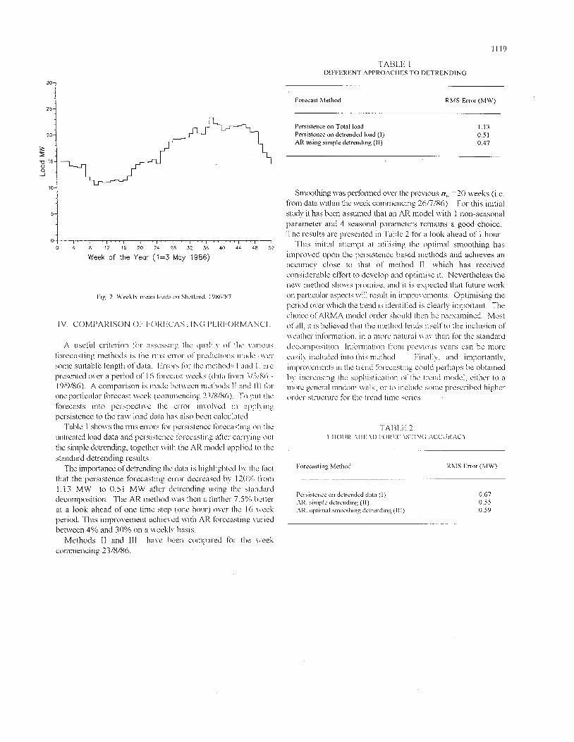
Fig. 1 sIio\vs an esaniple of a smc~othed curve fitted through onc year of wcekl!.. hourly mean load data at 1 .OO am, Saturday, fro111 Shctland

At this stage of the work no csplicit use is made of measured \vcather variations It is anticipated that inclusion of weather parameters would improve: the forecasting of the trend, indeed

1118

10-

5-

0

this could be considered the natural place at which to introduce these exogenous variables into the appsoach. It is considered that a good proportion of the fluctuations about the smoothed cu iw shown in fig. 1 can be explained by weathei- variation, and could, in principle, be incorporated into the trend model.

with a new smoothed cuve being calcu1:ited and forecast fonvard at each hour.

C. Srriiririary ofOvei.all Forecosting Tecliniqries

The resulting AR model takes the standard form

Ls(Mj,d,h) - ($lLs(~r7d,h-1) + ( $ & s ( ~ , d h 2 )

The algorithm developed is intended for real time application + . . ($pL,(M1dh-p> + @ 1Ls(M'7d9h-24) ( 1 3 )

+ (P&s(w7d&48) + ..@&LS(~j,d,h-24P) + a,

is weather sensitive. I11 addition to the seasonal patteius in the load there is a strong

diurnal trend \vhich exists because of the daily cycle of human

storage heaters which are conti-olled either by preset (by Scottish Hydro Electric plc) mechanical clocks or by mol-e recent radio

activih. The Shetland Islands possess a significant quantity of

. I . # 1 . , 1 1 I x / , I , I I I I I I I ' , , , , / , l ~ ~ ~ , ~ . , l ~ ~ , I , . , ( , , , I

The weekly load pattem or trend is updated and forecast forward using the contrasting methods of Sections IIA and IIB Subtracting this fiom the current hourly mean load, gives, together with previous values calculated in the same way, a time series representing the nominally stochastic residual load, sepresenting eiwythiiig not so far modelled. This detrended time sei-ies is found to be amenable to stwightfol-\vard AR modclling and can thus he predicted \\,it11 reasonahle accurac).. l'hc accuracy of this final prediction stagc is not critical once efl'ecti\,e detrending has been completed. It is for this reason tha t simple persistence forecasts of I-, can he used ivithout gi'eat loss in overall foi-ecasting accuracy.

Esanlination of the autocon-elation and partial autocon.el:ition functions for the time sei-ies L, indicated a season:il AR model to be appropriate.

where q$ i=1,2, ...p are the nonseasonal AR parameters, @a

i=1,2, ... P ai-e the seasonal AR parameters and 0, the usual white noise teim. A single seasonal teim with a period of 24 hours is suggested by the autocosselation function. By trial and error a model order of (1,4) was found to give the best performance, ie 11'1, H. Model parameters are identified using a standard least squares algoi-ithm; a data set looking four weeks backwards in time, i.e. I?,,. = 4, \vas found to give the best results.

Final forecasts are provided by summing the forecast trend and the fbrecast of L,

1 o sumniai-ise: threc soils of foi-ecasts can now be identified. ..

1 If rrf

persistence forecasting of standard detrended data AR foi-ecasting of standard detrended data AR fa-ecasting of data deti-ended by optimal smoothing

. - I he relative accuixcv ol'thcsc IS cxamined in section IV

1119

TABLE I DIFFERENT .4PPROi\CI IES TO DETRENDING

Forzcast hlcthod RMS Emor (MW)

Persistslice on Total load Pcrsislriicz oil dctrziided load ( I ) A R using siniple dctrsnding (11)

1.13 0.5 1 0.47

Smoothing \\:as peilbnnerl over the previous / I , + =20 weeks (i.e. tiom data \\<thin tlie \\,celi commencing 26/7/86). For this initial study i t has been assumed that an AR model with 1 non-seasonal parameter and 4 seasonal parameters remains a good choice. The results are presented iii l'alilc 2 for R look ahead of I hour.

This inilial attempt at iutilising tlie optimal smoothing has iiiipro\.cd upon the pcrsisttence hnsed methods and achieves an accur:ic!; close to tha t 01' method 11. which has received considerable ell'ort t o dc\~elop and optiiiiisc it. Nevertheless the ne\\- method sIio\\~s pi-omise, and i t is eipected that future \vork on pai~icular aspects \vi11 result in impro\,enients. Optiniising the pciicx1 o\w \vIiicli the trend I S identilied i s elearl\. inipoi-ttant. The choice 01' ARMA modcl OKICI . should then he i-cc\aiiiiiied Most o f all. i t is hclicved that the mcthod lends ~tsclfto the inclusion of' \ \ catliei. inlhi-mation. in ;I nxw n a t i i i - a l \I a!. than for tlie standai-d ~iccomposition Iiit1mii:ition ii-on1 pi-wious ycai-s can he morc GI si 1). i ncl udcd i n t o tli i s nic: t hod 1-i n a 1 I!;. and 1 in port an tl y , iiiipro\.cnicnts in the trend firecasting could perhaps he obtained 11y iiierc:isiiig the sol~liistication 01' the trend iiiodcl, either to a

<)i-dei- sti-~ict~re for the ti'cntl time series. 111orc gcllcl-al I - a n i l o i l l \\;:Ilk. 0 1 - to Ilicludc some pl-escl-ihcd higI1cr

l'elsislcllce 011 dell-ended tl;ll;l (I) . \ I< . simple deli-ending (11) .-\I<. optiin;il siiioothing dctreiidiiig ( I l l )

0.67 0 . 5 5 0.59

1120

V. CONCLIJSIONS

Renewed interest in load forecasting has provided the motivation to explore a new route foiivard to improved prediction. A novel and sophisticated method of detrending the data using optional smoothing has been outlined and preliminary results show it to be an effecti\re means of identifiring the trend, comparable in accuracy to already \veil developed techniques. It facilitated a reduction in the 1111s en-or of o\erall electricity demand prediction of 12%. compared to the method of persistence forecasting of data detrended using the standard decomposition.

It is considered that this init ial assessment of the smoothing technique for detrending analysis should provide ample justification for more detailcd studies to further improve the method, perhaps incoi-porating \\-eather information into the optimal smoothing algorithm

VI. ACKNOM'IJ<DGEMENTS

This woi-k arose fi-om a pi-oject jointl\. funded by the Science and Engineering Research Council and Scottish I-lydro Electric plc. Pal-ticular thanks are d t o the staff' of 1 .ei~\.ick Generating Station for thcir c collecting the electricity dcmand data and to D r .T A I~lnlliday of Rutherfoid Appletton 1,ahoratoi-y for assistance with the processing of the initial data. Gratitude is also espi-esscd to 1'1-okssor P C Young for introducing the authors to his iint-k on optimal smoothing.

M.A.Abu-El-Magd and N K.Sinha: Short-Tcnn l)eninnd Modelling and I:orcc:i.;tinf- A l?c\Gei\,. IEE l rans on S!stem Man. and Cybcmetics. Vol SMC- I ? . No. 3 . 1982.

D.W.Bunn and E.D.Famiet. (cds): Cnniparnti\:e modcls for Electi-ical Load Forecasting John Wile!. :ind Sons. I 9S5.

D. C. Hill, and D. G. Infield. " Modelling operation of the Shetland islands powci- s!'stem comparing computational and human operator's load forecasts", IEE Proceedings oil

Geiiei-atioi?, Truiisiiiissiori a r i t l Disti.ihiitioii; Vol 142, No 6; Nownber 1995. pp55.5-5.59

A. Piras: A. Gennond. 13. I3uchenel. K. Imhof> and Y. Jaccai-d: "Hetrogeneous Artificial Neural Network for short temi electrical load forecasting" IEEE T I Y T ~ . Poivei. Svs/eni,s, vol. 11, no I . I;ebruai?. 1996, pp. 397-402

H. Mori, and H. Kobayashi, "Optimal fuzzy inference for short-teim load forecasting", IEEE Trans. Power Systems, vel. 11, no. 1, February. 1996, pp. 390-396.

J. A. Halliday P. Gardner, G .A. Anderson, J. H. Bass, N. H. Lipman, N. L. Holding, J. W. Twidell, J. Cousins, "Simulation of wind integration for the Shetland medium- scale grid", Proc. ECWEC , Heming, Denmark. H.S.Stephens and Assoc., Bedford, UK, 1988, pp 518- 523.

C. N. Ng and P. C. Young, "Recursive estimation and forecasting of non-stationary time-series", Jtil. os Fowcnstirig, vol. 9, 1990, pp 173-204.

P. C. Young, " Fixed interval smoothing, regularisation and henderson detrending", CRES Tecknical Repol-r, TR97, Lancaster Ilniversity, 1993.

VIII. BIOGRAPHY

1)mkI Iiifirld w a s hom in Piiris. on 30th March. 1954. He was brought up :ind educated iti England. gaining a B.4 in Matheinatics from the University of 1,ancaster and a t'hD 111 Applied Mathematics from thr: University of Kent. He \vorked first for tlir: Building Services 1lese:arch and Iilfomiation Association on solni- themial system design, and then for the Rutherford Appletori Laboratory, on wind energy systems and electricity supply iiiodelliiig. He is iiow Director of CREST (Centre for Renewable Energy Systems Tecluiology)within the hqxiittiiait of Electronic and Elec?rical Engitieering at Loughborougli University, LJK.

T h ~ i t l llill \vas horn in the West h4idlatids on 2nd Janiiary 1964. He obtained h is 13 Sc i n hlatliwiatics at the IJiiivsrsity of Eseter and a M.Sc in space plasina physics lioni the liniversity of (h lord . He \vorked initially for a small eiigitiesriiig cotisull;uicy iii \\.itid energ) applications for two years before collaborating \\.it11 Ihvid infield oii 1111: ahove electricity dctiiaod forecasting pi-ohleiii. He tlicii \\orlied :it tlic School of Ocean Scieiice. University of Wales, I3niigor. dcwloping coiii1)iitiitiotiiiI niodcls of sedimait transport in coastal waters. l ie is no\v eniployed by the Lnviroiimental Systenis Science Centre of the Lini\,crsity of Re,ading. secondzd to tliz Proudman Oceanographic Laboratory T h i s project iii\dves assimilating satellite data into tidal models in a close collollalxvatioii with industrial pailtiers at the National Remote Sensing Centre Ltd.