opportunistic routing for indoor energy harvesting wireless sensor networks · ·...

Delft University of TechnologyMaster’s Thesis in Embedded Systems MSC

Opportunistic Routing for Indoor EnergyHarvesting Wireless Sensor Networks

Eloi Garrido Barrabes

Opportunistic Routing for Indoor Energy

Harvesting Wireless Sensor Networks

Master’s Thesis in Embedded Systems

Embedded Software GroupFaculty of Electrical Engineering, Mathematics and Computer Science

Delft University of TechnologyMekelweg 4, 2628 CD Delft, The Netherlands

Eloi Garrido [email protected]

16th August 2016

mailto:[email protected]

AuthorEloi Garrido Barrabes ([email protected])

TitleOpportunistic Routing for Indoor Energy Harvesting Wireless Sensor Networks

MSc presentationAugust 23, 2016

Graduation CommitteeProf.dr. K. G. Langendoen Delft University of TechnologyDr. Venkatesha Prasad Delft University of TechnologyDr. Zaid Al-Ars Delft University of TechnologyIr. V. Rao Delft University of Technology

mailto:[email protected]

Abstract

Internet of Things (IoTs) is envisioned to enable smart spaces such assmart homes, interactive museums or personalized trade in shopping malls.In these smart homes, several sensors and actuators assist in automatingtasks of daily life by forming wireless sensor networks (WSNs). Active andAssisted Living (AAL) is one of the important applications of smart homes,wherein activities of elderly persons are mainly monitored and assist themthrough actuators when required. With a huge number of sensors involved inAAL applications across smart homes, powering the nodes is an importantissue. To this end, make use of ambient energy harvesting technologies forenabling perpetual operations of the WSNs.

Due to limited energy harvesting opportunities in indoor environments,the energy levels of nodes in the WSN varies over space and time. There-fore, collecting data reliably over such a network is a significant challenge.There are many proposals in this domain, including MAC, routing, etc.,in such WSN. Although several routing protocols exist for WSNs and EH-WSNs, they do not consider the limited energy availability. Consequently,they do not adapt to the conditions, therefore fail in their objective. Wepropose a novel routing protocol called Harvesting Energy Aware Routingwith adaptive Duty Cycling (HEAR-DC), based on the philosophy of usingavailable energy, and routing the data packets opportunistically. HEAR-DChas several components: (i) transmitter-initiated MAC with opportunisticreception and duplicity avoidance; (ii) an energy harvesting aware gradient;(iii) adaptive duty cycling; and (iv) adaptations to support mobile nodesand sparse data traffic.

We also develop a trace-based energy harvesting simulation module forCooja, which does not exist as yet. With this module, real data traces canbe used for evaluating energy-harvesting WSN protocols. We present thedesign and implementation aspects as well as limitations of this module inthe current state.

We evaluate our protocol against the state-of-the-art opportunistic routingprotocol ORW. Results show that our proposed protocol achieves a latencyreduction of 64% with 92.75% lower packet loss as compared to ORW in thebest case of high energy availability. In the worst case, HEAR-DC achievesa substantial latency reduction of 37% and packet loss reduction of 48%compared to ORW. HEAR-DC achieves almost a factor of four lower delaythan ORW when only ‘events’ are transmitted.

Contents

1 Introduction 11.1 Challenges of EH-WSN . . . . . . . . . . . . . . . . . . . . . 41.2 Problem Statement . . . . . . . . . . . . . . . . . . . . . . . . 4

1.2.1 Challenges . . . . . . . . . . . . . . . . . . . . . . . . 51.3 Contributions . . . . . . . . . . . . . . . . . . . . . . . . . . . 6

2 Related Work 92.1 ORW . . . . . . . . . . . . . . . . . . . . . . . . . . . . . . . 102.2 ORiNoCo . . . . . . . . . . . . . . . . . . . . . . . . . . . . . 11

3 System Model 133.1 Network Architecture . . . . . . . . . . . . . . . . . . . . . . 133.2 Energy Model . . . . . . . . . . . . . . . . . . . . . . . . . . . 14

3.2.1 Energy Sources and Harvesters . . . . . . . . . . . . . 143.2.2 Storage Element . . . . . . . . . . . . . . . . . . . . . 163.2.3 Energy Consumption Model . . . . . . . . . . . . . . . 16

3.3 Assumptions . . . . . . . . . . . . . . . . . . . . . . . . . . . 17

4 Harvesting Energy Aware Routing Protocol with AdaptiveDuty Cycling (HEAR-DC) 194.1 Overview of HEAR-DC . . . . . . . . . . . . . . . . . . . . . 204.2 Transmitter-Initiated MAC . . . . . . . . . . . . . . . . . . . 214.3 Gradient . . . . . . . . . . . . . . . . . . . . . . . . . . . . . . 234.4 Adaptive Duty Cycle . . . . . . . . . . . . . . . . . . . . . . . 264.5 Operation of HEAR . . . . . . . . . . . . . . . . . . . . . . . 27

4.5.1 Bootstrapping . . . . . . . . . . . . . . . . . . . . . . 274.6 Steady State Operation . . . . . . . . . . . . . . . . . . . . . 29

4.6.1 Adaptations . . . . . . . . . . . . . . . . . . . . . . . . 30

5 Trace-based Energy Harvesting Simulations 335.1 Advantages of Trace-Based Simulations for EH-WSNs . . . . 335.2 Data Traces of Energy Arrival . . . . . . . . . . . . . . . . . . 345.3 Energy Harvesting Module . . . . . . . . . . . . . . . . . . . . 35

5.3.1 Design and Implementation . . . . . . . . . . . . . . . 35

v

5.3.2 Features . . . . . . . . . . . . . . . . . . . . . . . . . . 375.4 Limitations and Open Questions . . . . . . . . . . . . . . . . 38

6 Performance Evaluation 416.1 Methodology . . . . . . . . . . . . . . . . . . . . . . . . . . . 416.2 Scenarios . . . . . . . . . . . . . . . . . . . . . . . . . . . . . 426.3 Results . . . . . . . . . . . . . . . . . . . . . . . . . . . . . . . 43

6.3.1 High Energy Scenario . . . . . . . . . . . . . . . . . . 436.3.2 Low Energy Scenario . . . . . . . . . . . . . . . . . . . 456.3.3 Protocol Evaluation under Variable Traffic . . . . . . 476.3.4 Impact of Mobile Nodes . . . . . . . . . . . . . . . . . 47

7 Conclusions and Future Work 517.1 Conclusions . . . . . . . . . . . . . . . . . . . . . . . . . . . . 517.2 Future Work . . . . . . . . . . . . . . . . . . . . . . . . . . . 53

vi

Chapter 1

Introduction

As the world moves towards ubiquitous connectivity, not just between peoplebut also including objects or “things”, a huge surge is expected in the usageof Internet of Things (IoT) devices and end-user applications. Applicationsrange from simple monitoring of temperature to automatic climate and soilcontrol for agricultural applications and connected fridges that place or-ders for milk when milk is over. The information exchange between devicesis not only powering these innovative applications but also making tradi-tional elements smart. For instance, today a mirror tells the user about theweather [6] when he stands in front of it, shoes calculate how much the userhas walked, and a coffee machine keeps coffee ready in the morning becausethe alarm clock informed about the user waking up from bed. To enablesuch applications, the systems usually require “eyes” to obtain informationand learn, and “mouths” to talk to each other. Typically, sensors form theeyes to measure a physical parameter, and wireless radios work as the mouthto communicate data providing our applications with the required tools toadd the adjective “smart” to more and more fields every day.

One of the important applications enabled by IoTs is Active and AssistedLiving (AAL). AAL encompasses technical systems to support people dwell-ing in a smart house. In the past, AAL was conceived to support elderlypeople and individuals with special needs in their daily routine. The primarygoal of AAL was to maintain and foster the autonomy of those people. Thus,to increase safety in their lifestyle and in their home environment. However,recently, it has been extended for the well-being of any person, includingfor healthy persons [2]. The idea is to allow people to age healthily, so thata certain quality of life is met, specifically for the majority of older adults.AAL enables easier access to information to informal caregivers such as fam-ily and friends as well as the doctors about the activities of the person in anAAL enabled house. Specifically, with smart sensors deployed in the house,the person’s activities of daily living (ADL) can be monitored easily. Anyabnormality can be reported immediately to the caregivers.

1

To monitor ADLs and the other environmental parameters, many sensorsare deployed around the house. For instance, motion sensors to detect wherea person is, temperature and humidity sensors to determine the ambiance,wearables and body area sensors to determine respectively the activitiesand physiological parameters of the person. Fig. 1.1 shows an exampledeployment of the system in an assisted-living house with many residents.While some sensors may be fixed, wearables and other body sensors areworn by the person making the sensors mobile. These sensors are typicallypowered by batteries.

Figure 1.1: Assisted-living house deployment. Composed by emplaced nodesand body sensors.

All the data from the sensors need to be collected at a central placefor further processing. Alternatively, to conserve battery, only ‘events’ ofcertain significance may be reported [32, 31]. We call such systems as event-triggered systems. Events in an AAL scenario can be quite sparse dependingon the number of people in the house. For example, if the user is stationary,there is no change in the environment, hence there is no ssensor data toreport. However, when the user begins to move, the sensor may report thischange in value. This reduces the traffic as well as increases energy-efficiencyof the node.

Most of the wireless sensor nodes are small, inexpensive, low power con-suming devices that are powered by batteries. Typically, most AAL de-ployments need a multi-hop communication before the data reaches a ‘sink’,forming a wireless sensor network (WSN). The maximum number of hopsdepends on the deployment. More sensors are expected to be deployed inthe near future in order to gain fine-grained observations of ADLs in smarthomes. While WSNs have been researched for more than a decade now,energy efficiency and scalability with respect to gathering data for a given

2

deployment still attract the attention of researchers.Typically, the sensors deployed are required to last long. However, since

the nodes are battery-powered, their lifetime is limited. Much researchhas been done to enhance energy-efficiency of nodes through algorithmsand protocols to extend their lifetimes. However, it is impractical to havebattery operated nodes since replenishing them is a laborious task. If nodesare deployed in inaccessible locations, the network has a limited lifetime.Consequently, harvesting energy from ambient sources to power these nodeshas attracted attention in recent times. Energy harvesting is a techniquethat harvests or scavenges a variety of untapped ambient energy sourcesand converts the harvested energy into electrical energy to recharge storageelements such as batteries or super-capacitors [21]. Energy harvesting canpower the nodes perpetually in theory [29] and also it provides secondarybenefit of providing the context [31].

Figure 1.2: Indoor energy harvesting opportunities.

Energy-harvesting technology enables the network to extract energy fromsurrounding environment, such as solar power [12], mechanical movement [26],heat [13] and fluid flow [3]. Fig. 1.2 shows few opportunities of scavengingenergy in a home environment. Energy-harvesting technology provides nu-merous benefits [21]:

1. Reduce the dependency on battery power: with the harvested energy,nodes eliminate the use of battery power—the harvested ambient en-ergy may be sufficient to eliminate the need for batteries completely.

2. Reduce installation and maintenance cost: self-powered nodes elimin-ate service visits to replace batteries. This independence of each node

3

has the potential to boost its market potential into the consumer worldsince it needs the least intervention from end-users.

3. Provide long-term solutions: reliable nodes with energy-harvestingdevices will function as long as the ambient energy is available, whichis perfectly suited for long-term applications.

With untapped power sources, energy-harvesting wireless sensor networks(EH-WSNs) can operate perpetually. With EH-WSNs, our goal of collectingsensor data be it event-triggered or periodic data at a sink, reliably andperpetually should be realizable. However, it is not straightforward to do soas there are certain challenges.

1.1 Challenges of EH-WSN

Unfortunately, merely replacing the batteries with energy harvesters doesnot guarantee perpetual network operations nor the desired reliability. Thisis due to:

1. Ambient energy sources do not provide constant power. While theharvested energy can at times be very low, it can be in excess of thestorage capacity of the nodes on other occasions. For instance, statist-ics show that the difference in available solar power at shadowy, cloudyand sunny environments can be up to three orders of magnitude [30].

2. The harvested energy from ambient sources varies drastically by loca-tion and time. For example, consider one node placed next to a windowwith direct sunlight and the other one positioned in a bookshelf. Theamount of energy harvested by these nodes is different during day andnight. In either case, the node next to the window has more opportun-ities to harvest energy than the node in the bookshelf since the latternode probably cannot receive direct light on its solar panel.

These aspects are illustrated with the following example. Fig. 1.3(a) showsan EH-WSN in which all nodes have sufficient energy at time t1. However,due to insufficient harvested energy, node 3 dies at time t2. The networkis still connected through nodes 1 and 4. However, when node 1 dies at t3,the network gets disconnected. Therefore, a system that tackles this typeof situation and redirects node traffic dynamically is required.

1.2 Problem Statement

Evidently, the major problem is to collect data reliably over the dynamicnetwork, which is the focus of this thesis. We target to design a routingprotocol, along with a routing metric, for EH-WSNs that enables reliable

4

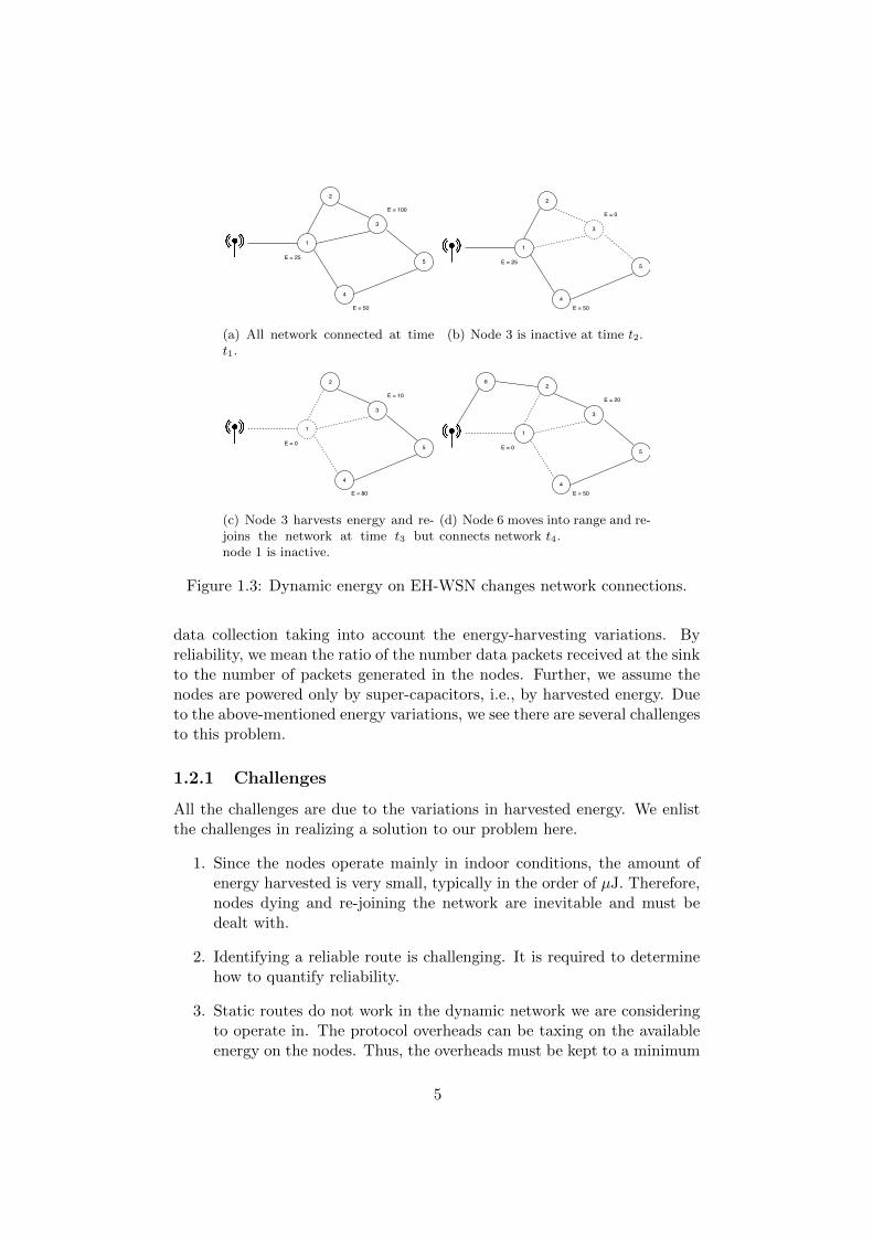
(a) All network connected at timet1.

(b) Node 3 is inactive at time t2.

(c) Node 3 harvests energy and re-joins the network at time t3 butnode 1 is inactive.

(d) Node 6 moves into range and re-connects network t4.

Figure 1.3: Dynamic energy on EH-WSN changes network connections.

data collection taking into account the energy-harvesting variations. Byreliability, we mean the ratio of the number data packets received at the sinkto the number of packets generated in the nodes. Further, we assume thenodes are powered only by super-capacitors, i.e., by harvested energy. Dueto the above-mentioned energy variations, we see there are several challengesto this problem.

1.2.1 Challenges

All the challenges are due to the variations in harvested energy. We enlistthe challenges in realizing a solution to our problem here.

1. Since the nodes operate mainly in indoor conditions, the amount ofenergy harvested is very small, typically in the order of µJ. Therefore,nodes dying and re-joining the network are inevitable and must bedealt with.

2. Identifying a reliable route is challenging. It is required to determinehow to quantify reliability.

3. Static routes do not work in the dynamic network we are consideringto operate in. The protocol overheads can be taxing on the availableenergy on the nodes. Thus, the overheads must be kept to a minimum

5

in order to make efficient use of the available energy on the nodes.Frequent updating of the nodes leaving and joining cannot be done,and a suitable low overhead workaround must be sought.

4. Mobile nodes add another dimension of dynamics to an already dy-namic network. The protocol must enable these nodes to send dataon this network reliably.

There are several energy-efficient routing protocols for WSNs in the lit-erature (e.g., CTP [15]). Most of these protocols have overheads for link-quality assessments and route maintenance. Opportunistic Routing (OR)based protocols avoid these overheads to a great extent [14, 37]. The twoimportant OR protocols in this context are ORW [14] and ORiNoCo [37].ORW is one of the most well-known OR-based protocol for battery-poweredWSNs, but does adapt to energy variations in EH-WSNs. ORiNoCo hasbeen adapted for EH-WSNs; however, it is passive in adapting to energyvariations. This is because ORiNoCo uses receiver-initiated medium accesscontrol (MAC) along with adaptive duty cycling1 to route packets than anactive routing metric. This results in packets getting stuck on high en-ergy nodes surrounded by low energy nodes with little progress. Therefore,we propose a novel OR-based routing protocol, Harvesting Energy AwareRouting with adaptive Duty Cycling (HEAR-DC), based on the philosophyof opportunistic use of available energy and wireless channel for routing. Inthis protocol, we make the high energy nodes take more load than the lowenergy nodes to achieve reliability. Furthermore, we propose a novel gradi-ent, or routing metric, that allows to actively make the higher energy nodestake more load. However, number of hops can vary also because of limitedranging based on the availability of energy. Sometimes it may be importantto send a packet twice on a short a link rather than sending once on a longerlink based on availability of energy.

1.3 Contributions

This work contributes to the state of the art in the following way:

1. We propose a novel OR-based routing protocol, Harvesting EnergyAware Routing with adaptive Duty Cycling (HEAR-DC), that providesa reliable routing solution for EH-WSNs.

2. We propose a novel gradient to quantify the reliability together withrouting progress offered by a node. We identify reliability with theenergy level of the node: higher the energy in the node, higher is the

1Adaptive duty cycling is a technique in EH-WSNs in which the ON period of the nodeis proportional to the energy present in the storage.

6

reliability offered by the node. The intuition is, because it has moreenergy, it can forward the packet sooner in the direction of the sink.

3. We develop an energy-harvesting simulation module for Cooja, whichdoes not exist as yet. This module uses real energy data traces onthe nodes to simulate energy harvesting rather than the conventionalmethod of using stochastic distributions. Simulations with this moduleis a step closer to reality.

4. We evaluate the system through simulations on Contiki OS with real-world energy harvesting datasets. We show that HEAR-DC achievesa substantial latency reduction of 37% and packet loss reduction of48% compared to ORW when the harvesting energy is low or none forsome nodes (worst case).

The major takeaways from this thesis are the following:

1. A novel gradient and routing protocol with low overheads that is de-signed to provide reliable data collection even in low energy harvestingconditions. This takes EH-WSNs a step forward since HEAR-DC doesnot rely on energy predictions or location information, and can workwith any kind of harvesting technology.

2. The energy-harvesting module for Cooja that enables trace-based sim-ulations, since the simulations are a step closer to reality.

7

Chapter 2

Related Work

Many routing protocols have been proposed for WSNs [28]. There is adifferent protocol for almost every scenario. Most of these works considerbattery-powered networks, wherein one of the inevitable requirements isenergy efficiency, i.e., maximize the lifetime of the network under a certainscenario. Most of the protocols carry overheads with them, such as controlpackets to maintain routing structures/parents in tree based protocols, andlink-quality assessment (e.g., Collection Tree Protocol [15]) in order to selectlinks of consistently high reliability and achieve higher energy efficiencies.

We studied several current EH-aware protocols from the literature [28].Some of the protocols introduce improvements. Protocols like RandomizedMax-Flow (R-MF) [5], Energy-opportunistic Weighted Minimum Energy (E-WME) [25] and Randomized Minimum Path Recovery Time (R-MPRT) [23]used the stored energy or a node’s harvesting ratio as metric parameter tofind a suitable route towards the sink. R-MF focuses to improve throughputbut needs information about the fill network; R-MPRT only uses harvestingrate as metric, which leads to oscillations. E-WME has lots of losses in lowenergy conditions and overheads produced by learning about neighborhoodstate [19].

The Opportunistic Routing (OR) paradigm, on the other hand, reducesoverheads and does not maintain routing tables, and provides highly energy-efficient, low-delay data collection possibilities [14]. OR works on the prin-ciple of anycast, i.e., the packet is broadcasted over the medium but is pickedup by a suitable forwarder while the other nodes drop the packet. In OR,the forwarding decision of a packet is delayed until after the transmission,thereby spatial diversity of the wireless channel is exploited. OR in WSNstarget energy efficiency and low overhead mechanisms for forwarder selectionin duty cycled radios.

In the context of our problem, OR paradigm suits the best since (a) weneed low overhead mechanisms to overcome the problem of nodes leavingand rejoining the network; and (b) it is best to delay the forwarder selection

9

until after transmission as the node with high reliability quotient can for-ward the packet. We base our solution on OR method as shall be describedin Chap. 4. We shall, therefore, summarize two important state-of-the-artOR based routing protocols - Opportunistic Routing in WSNs (ORW) andOpportunistic Receiver-initiated No-overhead Collection (ORiNoCo) proto-cols in this chapter.

2.1 ORW

Opportunistic Routing in Wireless sensor networks (ORW) [14] is an oppor-tunistic routing protocol that targets applications with low and asynchron-ous duty cycled radios. ORW introduces a new distributed routing metricnamed Expected number of Duty Cycles (EDC). This metric generates atree-like structure towards the sink based on the accumulated number ofDC through a particular path. ORW is a potential candidate for EH-WSNbecause ORW nodes forward their packets to the first suitable neighbor whois awake. Thus, it manages to reduce delay and energy consumption, and isresilient to link dynamics.

The metric, EDC, is computed using expected transmission delay andnode duty cycle, which is fixed across the network. The simplified formulaeach node uses to compute locally forwarding cost is given by,

EDC(i) =1∑

j∈F (i) p(i, j)+

∑j∈F (i) p(i, j) · EDC(j)∑

j∈F (i) p(i, j)+ ω, (2.1)

where the first term is the per-hop forwarding delay, the second termmodels the cost for the rest of the nodes and finally ω is the inherent cost offorwarding. p(i, j) is the probability of successful packet transmission fromover link (i, j) that is measured periodically using beacons or by passivelistening. Each node knows the price to forward a packet, its own DC andadds it to the received parent values.

To reduce the forwarding delay of packets, every node in ORW uses apool of parent nodes that can forward the packets. The forwarder set iscomputed by adding neighboring nodes sorted by their EDC in ascendingorder to the forwarder set until a pre-determined threshold EDC is reached.ORW mainly relies on overhearing of transmissions to update its neighbortable as well as link quality estimates.

ORW performs best when deployed in a high-density network where itcan exploit routing diversity to forward packets to the sink. However, ORWprotocol has not been strictly designed for EH-WSN. Therefore, some issuesarise when trying to use it in such scenarios. Firstly, ORW expects nodes tomaintain the fixed duty cycle which may not happen in EH-WSNs leadingto longer delays or packet losses. Secondly, packets must be periodically

10

exchanged in order to maintain link quality estimates and forwarder sets.This does not work well when event-based reporting is used. Furthermore,in this case, the EDC values age over time leading to rediscovery of routesbefore forwarding the packets.

2.2 ORiNoCo

Opportunistic receiver-initiated no-overhead collection (ORiNoCo) is an-other OR based protocol, designed for WSNs but has been adapted for EH-WSNs. ORiNoCo relies on two main components apart from OR, receiver-initiated medium access control (RI-MAC) and load adaptation or adaptiveduty cycling.

In RI-MAC, a low power probing method is used. That is, when a senderis ready to transmit, instead of sending, it waits until a receiver broadcastsa beacon. Once this beacon is received, and acknowledged that the receiverprovides routing progress, the transmission takes place.

In order to provide a reliable data collection route, ORiNoCo implementsan online adaptive duty cycling mechanism. Due to this, a node with moreenergy attracts more packets. When a node receives more energy, it increasesits DC, and hence an increased number of beacons are broadcasted. Thusthe possibility of the node to be selected as a forwarder increases. ORiNoCocan utilize Expected Transmission Count or hop count as its routing metric,though it does not explicitly recommend any. Hop count may be preferredsince it does not involve any link quality estimation overheads. In Fig. 2.1 wecan see an example of how ORiNoCo using RI-MAC works. As observed, thecommunication is initiated by the receiver which starts broadcasting beaconsto the channel and awaits a sender to acknowledge the transmission.

Figure 2.1: Communication in ORiNoCo [7].

Adapted ORiNoCo encounters some difficulties in more challenging in-door EH scenarios. Firstly, when there is excess of energy, beacons frommultiple nodes may collide. Although RI-MAC introduces some random-ness to avoid collisions, as density and energy level increase, the collisionsbecome unavoidable. Secondly, in the low energy scenario, when the energy

11

levels are low, the route chosen may not be reliable anymore since packetsget attracted to nodes with slightly better forwarding metric when the re-ceiver had energy. However, since the metric does not include any energyharvesting components in them, a good routing decision will not be made.We particularly address this aspect through our novel gradient.

12

Chapter 3

System Model

Two essential requirements for our AAL scenario: (i) the ability to be avail-able, i.e., be operational for extended periods of time, and (ii) scalable,i.e., be able to include more technologies (e.g., new on-body sensors) overtime. In this chapter, we shall describe a network architecture to supportsuch an AAL system which fits our study case. Furthermore, we shall alsospecify the energy models for the nodes since we consider all nodes to beenergy-harvesting.

3.1 Network Architecture

We depict a typical deployment of the AAL network in Fig. 3.1. The networkconsists of several heterogeneous devices - wearables and statically deployedwireless sensors - and a sink or a gateway node to collect and process the dataof activities of daily living. As shown in the figure, the nodes communicatewith the sink over multiple hops. As can be seen, each node can havedifferent energy levels.

Similar to AlarmNet [39], we consider two types of nodes: emplaced nodesand wearables or mobile nodes. The emplaced nodes are statically deployedin living spaces to measure temperature, light and other environmental para-meters along with assisting in determining a user’s activity. For example,emplaced nodes can detect if the user is in the vicinity of a sensor eitherthrough motion sensors or indirectly (e.g., through lights, water usage usingmicro-water turbines, etc.). The second goal of this static network is to actas a backbone network for the mobile nodes.

The location of emplaced nodes may be carefully chosen. However, withoutthe loss of generality, we consider the deployment to be random. The sizeof the deployment area in an AAL scenario, as expected, is less than manyoutdoor deployments (e.g., agricultural fields). Both the number of nodesand the number of hops may be limited depending on the actual size ofdeployment.

13

Figure 3.1: Network architecture composed by different emplaced nodesand wearables. Different colors indicate nodes being powered by differentharvesters.

The mobile nodes can either be part of a wireless body area network or anindividual wearable sensor that has to log data at the sink for further pro-cessing. They provide a variety of information either relating to physiologicalparameters, such as pulse rate, or activity data, such as from accelerometers,informing about the users movements. The position of the nodes varies asthe user moves within the house. Therefore, the mobile nodes would look tosend their data to one of the emplaced nodes for further routing or to thesink directly when possible.

3.2 Energy Model

To make the nodes operate perpetually, we consider all the nodes to bepowered by harvesting energy. In this section, we shall describe the har-vesters, storage elements and consumption model.

3.2.1 Energy Sources and Harvesters

We can have different harvesting sources to power the nodes. As mentionedin Chap. 1, in indoor deployments, a wide range of harvesting sources isavailable to power the nodes light, movement, water, vibrations, air andheat.

Emplaced nodes with photovoltaic (PV) harvester can make use of sun-

14

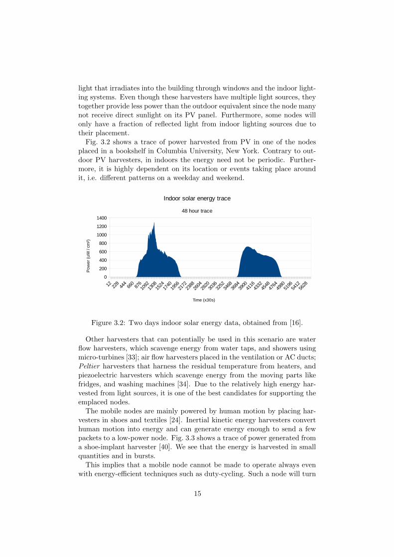
light that irradiates into the building through windows and the indoor light-ing systems. Even though these harvesters have multiple light sources, theytogether provide less power than the outdoor equivalent since the node manynot receive direct sunlight on its PV panel. Furthermore, some nodes willonly have a fraction of reflected light from indoor lighting sources due totheir placement.

Fig. 3.2 shows a trace of power harvested from PV in one of the nodesplaced in a bookshelf in Columbia University, New York. Contrary to out-door PV harvesters, in indoors the energy need not be periodic. Further-more, it is highly dependent on its location or events taking place aroundit, i.e. different patterns on a weekday and weekend.

Figure 3.2: Two days indoor solar energy data, obtained from [16].

Other harvesters that can potentially be used in this scenario are waterflow harvesters, which scavenge energy from water taps, and showers usingmicro-turbines [33]; air flow harvesters placed in the ventilation or AC ducts;Peltier harvesters that harness the residual temperature from heaters, andpiezoelectric harvesters which scavenge energy from the moving parts likefridges, and washing machines [34]. Due to the relatively high energy har-vested from light sources, it is one of the best candidates for supporting theemplaced nodes.

The mobile nodes are mainly powered by human motion by placing har-vesters in shoes and textiles [24]. Inertial kinetic energy harvesters converthuman motion into energy and can generate energy enough to send a fewpackets to a low-power node. Fig. 3.3 shows a trace of power generated froma shoe-implant harvester [40]. We see that the energy is harvested in smallquantities and in bursts.

This implies that a mobile node cannot be made to operate always evenwith energy-efficient techniques such as duty-cycling. Such a node will turn

15

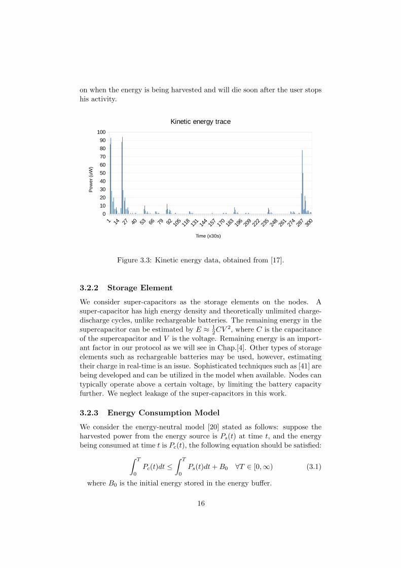
on when the energy is being harvested and will die soon after the user stopshis activity.

Figure 3.3: Kinetic energy data, obtained from [17].

3.2.2 Storage Element

We consider super-capacitors as the storage elements on the nodes. Asuper-capacitor has high energy density and theoretically unlimited charge-discharge cycles, unlike rechargeable batteries. The remaining energy in thesupercapacitor can be estimated by E ≈ 1

2CV2, where C is the capacitance

of the supercapacitor and V is the voltage. Remaining energy is an import-ant factor in our protocol as we will see in Chap.[4]. Other types of storageelements such as rechargeable batteries may be used, however, estimatingtheir charge in real-time is an issue. Sophisticated techniques such as [41] arebeing developed and can be utilized in the model when available. Nodes cantypically operate above a certain voltage, by limiting the battery capacityfurther. We neglect leakage of the super-capacitors in this work.

3.2.3 Energy Consumption Model

We consider the energy-neutral model [20] stated as follows: suppose theharvested power from the energy source is Ps(t) at time t, and the energybeing consumed at time t is Pc(t), the following equation should be satisfied:∫ T

0Pc(t)dt ≤

∫ T

0Ps(t)dt+B0 ∀T ∈ [0,∞) (3.1)

where B0 is the initial energy stored in the energy buffer.

16

As an implication of this model, a node wakes up when it has the energyto operate for a minimum period. Therefore, the nodes wake up asynchron-ously. Nodes try to maintain a certain duty cycle if the energy in the buffersupports the operation.

3.3 Assumptions

We make two simple assumptions in this work: (a) we assume the networkof emplaced nodes is initially connected, (b) we consider the radio channelsto be symmetric, i.e., if node u can send a message to node v, then v cansend a message to u, and (c) the mobile nodes always move within the rangeof at least one emplaced node.

17

Chapter 4

Harvesting Energy AwareRouting Protocol withAdaptive Duty Cycling(HEAR-DC)

There are several well-known routing protocols for sensor networks in theliterature (e.g., CTP [15]). Most of these protocols have overheads forlink-quality assessments and route maintenance. Opportunistic Routing(OR) based routing protocols avoid these overheads to a great extent [37].ORW [14] has been proposed for battery powered sensor networks andORiNoCo [37] has been adapted for EH-WSNs.

The amount of energy in the buffer on an EH node that uses the abovementioned OR protocols is influenced by four factors:

1. the rate of sending and receiving packets,

2. the rate of harvesting energy,

3. the rate of beaconing of the low-power MAC, and

4. duty cycle of the node.

The first two factors can only be passively measured by a sensor node.The second two factors can be controlled, and these factors influence thenode outage1, End-To-End delay, and packet losses. In this chapter, we de-scribe the design of our routing protocol, Harvesting Energy Aware Routingprotocol with adaptive Duty Cycling (HEAR-DC), that is based on OR,and uses harvesting and residual energy levels actively to enable reliable

1A node outage is said to occur when it runs out of energy to participate in networkactivity.

19

data collection. We provide an overview of HEAR-DC in Sec. 4.1. In thesections that follow, we describe the communication process in Sec. 4.2, thenwe describe our novel gradient (routing metric) in detail in Sec. 4.3, and fi-nally the bootstrapping and steady-state phases of the protocol in Sec. 4.5.1and Sec. 4.6 respectively. Finally, in Sec. 4.6.1 we introduce adaptationsto HEAR for including mobile nodes and operating when the packets aregenerated sparsely.

4.1 Overview of HEAR-DC

There are four main components that make HEAR-DC2 tailor-made for EH-WSNs.

1. Transmitter-Initiated MAC with Opportunistic Reception and Duplic-ate Avoidance: HEAR-DC uses a variant of Box-MAC-2, an asyn-chronous, transmitter-initiated low-power listening MAC with highenergy-efficiency. Furthermore, we enhance the protocol with the fol-lowing tweaks: (a) when a node has a packet to transmit but finds an-other on-going transmission, it opportunistically listens to the packetif that packet can be forwarded. This can reduce the end-to-end delay.(b) If a node finds out that a packet in its queue is being forwarded byits neighboring node, then it does not forward the packet to preventduplication.

2. Gradient : An ‘active’ gradient or routing metric that includes theresidual energy and harvesting rate of a node and is used so that thepackets are routed through nodes with high energy levels. This offersmore reliability, i.e., lower packet losses.

3. Adaptive Duty Cycling : Nodes adapt their duty cycles according tothe energy levels present in their super-capacitors. This makes thehigh energy nodes attract more load towards themselves which canagain influence the reliability and end-to-end delay.

4. Mobile Nodes and Sparse Data: Mobile nodes run a light-weight ver-sion of the protocol, i.e., they act just like data sources. They look toforward packet to any nearby emplaced node or the sink. Since eventsin a residential setting are rather sparse, the network must be ableto send this data. Most OR protocols include aging of their routingmetric, leading to larger end-to-end delays and less reliable routes. Wepropose to overcome this effect by introducing dummy packets withvery low rates when there is no traffic for a considerable duration.

2The version of our protocol without adaptive duty cycling is called HEAR.

20

4.2 Transmitter-Initiated MAC

The communication mechanism that allows our protocol to collect inform-ation is based on Opportunistic Routing. This means that all informationexchanges are based on anycast communication primitives. There are norigid transfer structures (e.g., routing tables) set. Therefore, any node canforward a packet as long as the gradient of the receiver is lower than thesender. An example is shown in Fig. 4.1, wherein the packet of node 1 isreceived and forwarded by nodes 2 and 3 in the direction of the sink. The

Figure 4.1: Anycast based forwarding.

medium access control employed is transmitter initiated and is a variant ofBox-MAC-2 [27]. Here we shall describe our method and not contrast withBox-MAC-2.

The communication between two nodes will always be initiated by a nodethat has a packet to send in its queue (sender). This node first does a clearchannel assessment (CCA) for the duration of a tinter−strobe to avoid anycollisions with on-going transmissions. If the CCA indicates the medium isbusy, then an opportunistic reception mode is invoked (this will be describedin Sec. 4.6). If the medium is free, then the node begins to send beacons,which we also refer to as strobes. After every strobe, the node waits for anACK from one of its forwarders with a lower gradient. The beaconing isrepeated until a receiver node successfully acknowledges the packet or thesender has reached the maximum transmission duration marked by top.

If a node receives a beacon and is a suitable forwarder, then the node willsend an ACK. However, before sending the acknowledge packet to the sender,the node employs a collision avoidance mechanism, i.e., it waits for a guardtime tguard = rnd([0, Tguardmax ]). The goal of holding the transmission backis to give time to other possible forwarders to acknowledge the packet. Bysetting a randomized time to reply, the chances of both forwarders answeringat the same time instant are reduced. Furthermore, if the node hears ACKfrom another forwarder, then the packet is not ACKed by this node anddropped from its queue to avoid duplication. This mechanism is shown inFig. 4.2.

The timings of strobing are indicated in Fig. 4.3. tstrobe is the time foractual air-time of the packet. tinter−strobe is the inter beacon period. trx−tx

21

Figure 4.2: Collision prevention mechanism. Receiver 2 drops the packetafter overhearing receiver 1 acknowledges it first.

is the time required to change the radio from receive mode to transmit mode,and ttx−rx is the time required to change the radio from transmit mode toreceive mode. These numbers can be easily determined and used to calculatethe number of strobes that can be done with a particular ON period of thenode.

Figure 4.3: Strobe timings.

We use a common frame format for all packets - beacons and acknowledg-ments - since we assume the packet length to be small and to keep it simple.This structure is shown in Fig. 4.4. By modifying the ‘TYPE’ field, a nodecan indicate if the frame is a strobe or ACK. The ‘GRAD’ field containsthe node’s gradient value. This value is also piggy-backed by the receiveracknowledging the packet. All the listening nodes will update this value,which will be described in detail in the following section. The ‘DATA’ fieldcontains the actual data. ‘TTL’ is used for statistical purposes (to keeptrack of packet path). Finally, the ‘DST’ field is used either to send thepacket into the sink’s direction or to mark which node a particular ACK isaimed at.

Figure 4.4: Packet field structure.

22

4.3 Gradient

The core element on our protocol is the novel gradient, which is tailor-madeto operate in EH-WSNs. The gradient is a routing metric that allows eachnode to decide if a packet is traveling in the right direction.

The connotation of what is the ‘best’ route in EH-WSNs is debatable. Thisis mainly because of energy variations in the nodes due to energy harvesting.Using hop-count as gradient gives the shortest route, but packets may notreach the sink. EDC metric of ORW does not take the energy variations intoconsideration, also leading to packet losses. Therefore, in our context, wedefine the most reliable route (i.e., most number of packets being delivered)between the sink and a node as the best route. Instead of computing the bestroute may require gathering knowledge about the energy levels, harvestingrate and the number of packets in its queue at a central location, we shallbuild a route online using the gradient.

In our design, we try to shift the traffic to the nodes with higher energyvalues. The purpose in doing so is to boost the chances of a packet reachingthe sink successfully, by hopping over reliable nodes. The key parametersthat affect this metric value are (a) position in the network; (b) residualenergy; and (c) energy harvesting rate.

Using these parameters, we construct our novel gradient as given in Eqn. 4.1.

gradientn = MIN(gradn + ρmax/ρ+ σ,GRADmax), (4.1)

where gradn is the average gradient of the neighboring nodes that forwardedthe packets of node n. ρmax/ρ is the inverse of the normalized value of thecurrent duty cycle of the node, and σ indicates the node’s harvesting state.And GRADmax is a constant defining the maximum value the gradient canhave.

The gradient of the sink is initialized to zero. Therefore, the first hopnodes will have a very low average gradient. This value increases continu-ously as the distance from the sink increases. However, nodes with higherenergy values will have slightly lower gradient due to energy-related para-meters (second and third parameters in Eqn. 4.1). This makes the nodeswith higher energy levels more attractive than the lower energy level nodes.

A node harvesting energy can buffer the energy and be operable for sev-eral slots, making the node more reliable than a node with an equal amountof residual energy. Furthermore, if low energy level nodes surround thisnode, then the route is not reliable, and the packets are likely to be lost ordelayed. This aspect is incorporated due to the average gradient, hinderingnodes from choosing this route. We call this an ‘active’ metric since energyparameters of a node are made known its neighbors as described in the pre-vious section, and therefore can make them part of the forwarding decisionfor a packet. This is in contrast to ORiNoCo. Wherein the energy relatedparameters are not disseminated, and high energy node attracts packet only

23

because of its adaptive duty cycling mechanism. In the situation of a highenergy node being surrounded by low energy nodes, the packet will mostlybe lost in ORiNoCo.

An example of the slope created by the gradient dissemination is shownin Fig. 4.5 exemplifying a situation where a longer route presents a loweraccumulated gradient due to different residual energy. The forwarding costof each node depends on the current state of a particular node, and the pathto the sink is composed by the addition of those forwarding costs. In somecases, a node would forward a packet through a worse route if the receivernode awakes before other better nodes. This case can be observed in thenode right of the origin. However, after the gradient has stabilized a nodewill pick only those routes that have lower gradient than its own.

Figure 4.5: Routing with gradient. Dashed lines mark the accumulated costthrough that specific path and the node value its forwarding cost.

The parameter ρ represents the duty cycle of a node. In case the nodeemploys an adaptive duty cycle that is proportional to its residual energy,this value ρ gives the indication of residual energy in the gradient. Eachnode computes its DC at the beginning of each operation cycle and thennormalizes this DC dividing it by the maximum fixed DC. By using theinverse of this value (i.e., ρmax/ρ), nodes with better power capabilities willpresent a lower gradient value, and thus, be more attractive to its neighbors.In case the node employs a fixed duty cycle, this ratio is constant over timeand acts a fixed forwarding cost.

The remaining parameter, σ, maps the harvesting state of a node into itsmetric. As ρmax/ρ represents the long-term energy fluctuations of the node,σ indicates the short-term energy capabilities of the node. The method tocompute σ aims to account for the harvest variations of each node by en-capsulating an average of recently collected values from a particular nodeinto a node harvesting state (NHS). Its goal is to represent the future energy

24

tendency of a node. This NHS value is not a static value, but is dependenton the time and the harvester type used by the node. With such value,a node will be able to modify its behavior to adapt to its future energystate, making a node’s metric more or less appealing to others dependingon a snapshot of its harvesting history. Thus, nodes that are seeing theirharvesting rate (HR) being reduced will redirect part of its traffic to neigh-boring nodes. Contrarily, if they start harvesting at higher rates, they willexpose themselves to the networks as better forwarders.

We compute NHS as NHS =∫ t+Tt tPcdt∫ t+Tt tPsdt

. The outcome of this operation is

either a value bigger than one when consumption is greater than harvesting,or a number between zero and one when a node has a higher energy inputthan the quantity it is using. We call it state LOW in former case andstate HIGH in the latter case. Both LOW and HIGH are assigned a valuethat acts as forwarding cost (e.g., LOW is given 3 and HIGH is given 1).This value is what we define as σ, which is a step-like, natural projectionof the value NHS. Therefore, a node with a HIGH state will have a bettergradient than a node with a LOW state. With this differentiation, we shifttraffic from nodes with worse harvesting parameters to those with betterprojection.

Hysteresis. A node’s NHS state can oscillate depending on the amountof energy being harvested. Therefore, to reduce oscillations due to rapidpower fluctuations a hysteresis mechanism has been added to it. Instead ofchanging σ the same moment a node reaches a certain value, depending onthe direction of the charge, it will compare its value with a higher or lowerthreshold, reducing the noise a node can experience when exposed to burst,fluctuating energy sources.

With this method, nodes that just briefly start harvesting more energywill not endanger its operation state by fluctuating to a higher σ and willnot attract much traffic. The same approach applies when comparing with alower state. Nodes that had a transitional energy fading won’t automaticallyjump to a lower σ.

Aging. A node’s gradient not updated after certain duration may nolonger hold due to the energy variations. Therefore, an aging mechanismhas been incorporated to degrade the node’s gradient. When a node usesthe gradient value of a forwarder node, the sender node notes the amountof time used to establish the connection with that forwarder as rendezvous-time (RVt). After the average gradient is computed, the RVt is used to setan aging prevention window for that entry. This window defines an agingprevention time for each of those entries.

Therefore, each entry has a different age prevention time before it startsto age, substituting first those connections of worse quality and maintaininga better gradient overall. This age prevention time is defined as a naturalnumber of wake cycles before the metric starts the degradation process.

25

Figure 4.6: Aging and age prevention mechanism. Marked in red are theentries that are currently degrading its value. In gray color is set the ageprevention number of iterations left.

With this technique, a node that finds that its neighboring nodes presentworse gradient values than its own, will eventually degrade its gradient andreestablish the connection with the network. In Fig. 4.6 we can see anexample of the aging and age prevention mechanism. Marked in red thoseentries that have reach age prevention value zero and will start to degradeand in gray those that still have iterations left.

Extreme situations occur when a section of the nodes has not forwardedany packet for a long duration. The gradient in every node ages and thenetwork has to re-initialize. To avoid such a situation, each node generates adummy packet with very low probability and forward it to update gradiententries.

4.4 Adaptive Duty Cycle

The duty cycle (DC) of a node is the ratio between the duration of time it isawake and duration of time it is in the sleep state. It is possible to adapt theduty cycle of a node proportional to its residual energy level. Adaptive dutycycling are advantageous for the following reasons: use the surplus of energyfrom the high harvesting nodes to attract more traffic and reduce end-to-end delay by keeping nodes awake for longer and therefore, increasing thechances to meet other nodes.

We implement the adaptive duty cycle method as proposed in [38]. Inthis method, the duty cycle duration is modeled as a control system. Theobjective of the control system is to minimize the distance between thecurrent battery level to a set point, and the control variable is the dutycycle that is varied depending on the distance. This system can be modeledas a discrete, first order, linear dynamic system, and the problem can beformulated as a linear-quadratic (LQ) tracking problem. The model of thesystem is presented in Eqn. 4.2.

26

yt+1 = ayt + but + cwt + wt+1, (4.2)

where y is the duty cycle output value to correct the deviation, u is thecontrol variable, w is a mean zero input noise and a, b, c ∈ < are discretestep coefficients. The objective of the controller is to maintain the averagevalue of |yt− y ∗ |2 as small as possible over infinite time horizon as given inEqn. 4.3. Here y∗ is the desired set value.

limN→∞

1

N

N∑t=1

(yt − y∗)2 (4.3)

We use iteratively the optimal control law 4.4 that minimizes Eq.4.3 toobtain the appropriate duty cycle output value for a specific node.

ut =y∗ − (a+ c)yt + cy∗

b(4.4)

Solving for ut in Eqn. 4.2 is not straightforward because the coefficients usedin the process are not known a priory. In order to estimate the coefficientsand solve for ut as in Eqn. 4.4, a gradient descent technique [22] is proposed.This mechanism results in the definition of a parameter vector and an it-erative approach to computing those values online. We refer the reader to[38] for the algorithm.

We tested the DC controller in a stand-alone code with an input of 24hours of real solar data from Columbia University. Fig. 4.7 shows how theduty cycle adapts to the residual energy in the node.

We set the duty cycle to be within [ρmin, ρmax]. By including this adaptiveDC mechanism into our system, we aim to boost the duty cycle of each nodeto the maximum possible, so that each node will increase its ON durationfor as long as its energy capabilities allow it. This will keep those nodes withbetter energy level to operate for longer durations and therefore, attract abigger part of the network traffic to them. We shall call the version of HEARthat incorporates adaptive DC as HEAR-DC.

4.5 Operation of HEAR

In this section, we shall describe the operation of our routing protocolHEAR.

4.5.1 Bootstrapping

In the beginning, each node sets its gradient to the maximum. With thisvalue constant over the network, no data collection is possible because nonode knows their position in the topology. Each node generates some dummypackets at this phase to compute its gradient to the sink. At this instance,

27

(a) Solar energy harvested.

(b) Adaptive duty cycle variations.

Figure 4.7: Adaptive DC controller output to EH input.

each node, when awake, will broadcast its payload. However, because everynode has the same gradient, no exchange will take place. This phenomenonapplies to all nodes except those nodes located within the communicationrange of the sink.

The 1-hop away nodes will receive an acknowledgment from the sink,which has a gradient 0. After these nodes update their own metric withrespect to the sink, they will have a lower gradient value than the rest ofthe network. This process repeats for the second hop nodes and continuesto update the rest of the network. The computation of gradient has beenexplained in Sec. 4.3.

The bootstrapping phase is said to end when every node has a gradientvalue smaller than its initial value, and is more or less steady for a durationof time. After this, the node can switch to the steady state operation phase.In our implementation, we do not explicitly mark the phase boundaries.However, a node does not forward a packet if its gradient is maximum.

28

4.6 Steady State Operation

During the steady state operation phase of a node, the node repeats a set ofoperations each time it wakes up. The first step is to estimate the amount ofremaining energy and saves it into memory to compute the harvesting ratefor future iterations. Then it computes the harvesting rate and updates theσ value of the gradient. Next, the node computes the duty cycle it canoperate in. For HEAR, we set it ρmin always, while HEAR-DC calculatesthis value using the method described previously. The duty cycle will setthe operation duration, top which defines the maximum amount of time anode can stay awake before going to sleep.

After the required parameters have been defined, the node computes itsgradient. It then enters the main loop, which can be observed in Fig. 4.8.The node will remain in this loop until the node sleeps (i.e., top is notreached). The first action taken by the node is to check if its queue containspackets to forward or not. If there are packets in the queue waiting to beforwarded, the node enters a transmission phase. Otherwise, it would startlistening for incoming transmissions.

Figure 4.8: Main operation loop diagram.

In the transmission phase, the node probes the channel for currently on-

29

going communications (CCA). In this step, two scenarios can happen. If thechannel is free, the node can proceed to strobing. However, if the channel isoccupied, then the node will perform opportunistic reception. That is, thenode will try to receive the on-going transmission. In case the node is a suit-able forwarder for the received packet, then the node will try to acknowledgethe transmission and add the packet to its queue. During the opportunisticreception, if the packet is not successfully received, then the node wouldwait for the channel to become available. The amount of time the node canwait for the channel to become free is equivalent to the inter-beacon timetinter−strobe.

In case the node starts the beaconing process, the node stops beaconingin two conditions, whichever happens first. Either top reaches the maximum,or the packet is ACKed successfully. However, if the node has received anACK and some ON duration is still available from the time set by top, itloops again to find if there are packets in its queue.

As stated above, if a node does not have queued packets to transmit, it willenter a listening phase. In this phase, the node waits for incoming transmis-sions. In the favorable case that the node overhears a communication, and itcan provide routing progress, then node acknowledges the transmission andadd the packet to the queue. Similarly to the sending phase, the listeningphase has two exit conditions. First, the main condition imposed by thetimer top being over, and secondly, successfully receiving and acknowledginga packet transmission. After either condition is met, the node will, in thecase of having remaining available time, go through the main loop again.

4.6.1 Adaptations

We propose two adaptations to HEAR for making the network operate welleven when the packets are generated sparsely and accommodating mobilenodes. We describe them in this section.

Sparse Data

In a residential setting, at times there are no events to be reported for longdurations. For example, during night times there are usually no events toreport. The gradient, as described in Sec. 4.3, ages over time. Over asufficiently long duration with no packets in the network, the gradient canreach the maximum value. This would necessitate a bootstrapping phaseagain, which is a costly process. Therefore, nodes generate dummy packetswith a low probability once the metric in a specific node starts experiencingcertain degradation. With this technique, when the network works under areduced traffic, instead of undergoing a general gradient degradation due toaging, each node participates actively in maintaining that gradient.

30

Mobile Nodes

The system has been dimensioned to be able to operate under low energyparameters and sparse traffic. These features allow us to include mobilenodes in the network without much difficulty. Mobile nodes maintain a non-initialized metric for their whole operation duration. They opportunisticallytransmit their data to any emplaced node in their vicinity. Moreover, be-cause mobile nodes cannot forward packets from other nodes due to theirnon-initialized metric, they use all their energy in transmitting their packetswhenever the channel is free.

31

Chapter 5

Trace-based EnergyHarvesting Simulations

In this work, we have developed a module for Cooja that allows for simu-lating energy-harvesting on a sensor node, and hence the network, by usingreal data traces. This module is generic and straightforward to use, andcan easily enable close to real-world EH-WSNs protocol evaluation. In thischapter, we describe this module in detail before moving on to evaluatingHEAR.

We begin with listing the advantages of using real data as the energy inputfor simulations in Sec. 5.1. Next we describe our module in detail in Sec. 5.2and 5.3. Finally, in Sec. 5.4 we summarize the implications of taking thisapproach and present some open questions about trace-based simulations.

5.1 Advantages of Trace-Based Simulations for EH-WSNs

Most protocol evaluations for EH-WSNs today are being done by simula-tions [4], while only a few of them are deployed in real-world with harvesters.This is done since real-world evaluation has several disadvantages: (a) eachnode should have a harvester built, which implies high cost to deploy; (b)it takes a long time to evaluate in all conditions (for e.g., one year for asolar harvester to cover all seasons); (c) a dense network is required to covermany locations as energy harvesting varies over locations; (d) node andsoftware failures must be monitored and handled quickly; (e) data collectionfrom a large network could be challenging in real-time, and (f) experimentrepeatability is challenging.

Furthermore, most simulations use stochastic distributions for energy ar-rivals, which is not the reality. Stochastic distributions fail to capture burstsof energy arrival, correlated energy arrivals for one node and among neigh-boring nodes. Moreover, implementing a stochastic distribution on a real

33

node is further approximated due to limited floating-point computation cap-abilities. A data trace-based simulation, on the other hand, is much closerto reality.

Considering all these factors, we designed a simple battery module thatprovides trace-based energy arrival. The simulations thereof have the cap-abilities of (a) being fast, (b) evaluating in conditions close to reality, and(c) allowing repeatability of experiments. Since Contiki is a popular OS forWSNs and Cooja is its simulator, we wrote the EH module for Cooja.

5.2 Data Traces of Energy Arrival

In this section, we shall list a few datasets for a variety of harvesters anddeployments that we can make use of in our EH-module.

1. Outdoor solar data trace is the simplest to obtain since meteorologicaldepartment across the world save the solar irradiance (W/m2) val-ues. Smart-grid initiatives further fuel data collection, initiating othersources (such as CONFRRM [10] in the USA) to collect solar data aswell.

2. Indoor PV harvesting data trace in five different setups have beencollected by Columbia University, New York and made it availableonline [16]. The five setups are (a) student’s office, south-facing, 6thfloor, located on a windowsill. (b) Same as (a) but placed on book-shelf far from a window. (c) Departmental conference room, large win-dows and unobstructed view. (d) Student office; corner window facingSouth and West, extensive shading used.(e) Student’s office; setup on awindowsill with window usually open, receives unattenuated reflectedoutdoor light.

3. A shoe-implant harvesting data has also been collected by ColumbiaUniversity, New York and also has been made it available [8]. Thisdata has been collected by five people over several days each with aparticular profile. The participants were asked to carry the sensingunit over a period of 25 days, and they used different commute andtransportation means: foot and train. This data allowed to generatetraces over a 24-hour period. The dominant motion frequency of thecollected traces falls between the range of 1.92-2.8 Hz, which corres-ponds to human walking. This data is then converted into energyfollowing the process described in [18].

At this time, the number of such traces is limited but we expect it toincrease as more and more deployments of EH-WSNs will be done.

34

5.3 Energy Harvesting Module

5.3.1 Design and Implementation

In this section, we describe the design process and the implementation detailsof the Energy harvesting Module. An application is designed to use energytraces on Contiki’s Cooja simulator.

1. The EH-model is used as an external module to Contiki’s stack. Asshowing in Fig. 5.1. The HEAR application can invoke and use theEH-Module. Initializing the stack is easily accomplished by importingthe source code and call the core Contiki structures in the node’smain code. Contiki applications are built upon the Contiki Netstack.The Contiki Netstack can be observed in blue in Fig. 5.1. In theimplementation of the HEAR protocol, we overwrite and merge thedifferent stack modules in a way we can control at low level the node’sbehavior. The HEAR protocol is composed of two main blocks: HEARapplication (gray) and the energy harvesting module (yellow).

Figure 5.1: Contiki Netstack based on [9] and HEAR block diagram.

2. The energy harvesting module works as a separate program from themain node code and is organized in three sub-modules: harvesting,storage, and consumption. A block diagram of their dependencies canbe observed in Fig. 5.2.

• Harvesting : This sub-module is in charge of managing the node’sinput energy. The first action is to load values from a trace fileinto memory. Once these values have been used, the harvestermodule will reload the next energy trace values into memory. Toobtain the energy values the harvesting module needs access to

35

Figure 5.2: Energy harvesting module block diagram.

the energy file uploaded into the node. To do so, it uses the CoffeeFile System of Contiki environment. The module will provideperiodically a certain amount of energy to the node and enabletrace-based simulation.

• Storage: The storage sub-module manages the access to the sharedenergy variables. This sub-module is the link between the har-vesting module, the consumption module, and the HEAR applic-ation. All the energy information is stored in several variables likethe remaining energy, harvesting rate, consumption rate, and soon. The storage module ensures that different modules are notaccessing the same variable at once with semaphores as well asvalidates that a node is not overflowing the supercapacitor stor-age capacity or depleting it below empty.

• Consumption: The last sub-module uses the Energest (Contiki’senergy estimation mechanism) information to calculate the amountof energy used by each node component, i.e. radio transmitting,radio receiving, CPU, and so on. This module receives the num-ber of clock ticks from each element. These ticks increase whena particular element has been turned ON. All the different tickvalues are periodically collected by the consumption sub-modulewhich computes the total consumption value depending on thesource of each tick, i.e. the radio or CPU. Finally, the energyvalue is removed from the remaining battery and the energy stat-istics updated. Moreover, the system can isolate the managerthread and remove its consumption from the total, accountingonly for the node operation consumption.

3. To use the energy harvesting module to simulate with real datasetsthe user need to perform several actions:

• Sampling frequency : The user needs to configure how often en-ergy is harvested by the HEAR application. This is the frequency

36

with which the file will be read and the energy is ‘harvester’. De-pending on the data granularity of the file, the energy harvestingmodule will be able to access it at a different rate. In our simu-lations, the harvesting rate has been set to sample each 10 ms.

• Energy file: The selection of the file each node will use is definedin a Cooja simulation script. To upload such file it can either beselected manually via the Cooja’s CFS user interface or scriptedwith Rhino-Javascript. The following sniped exemplifies the fileupload script:

m = sim.getMote(i);

FILEPATH = "/home/user/energy_traces/cfs_file.txt"

int = m.getInterfaces();

fs = m.getFilesystem();

success = fs.insertFile(FILEPATH);

• Once the file it is uploaded successfully into each node, then thenode energy harvesting module has to initialize the file systemand set the initial trace pointer. The address of the pointer canbe randomized to add variation to the simulation. This allowsseveral nodes to use the same energy file and still present differentbehavior. The interaction with the Coffee File System is donevia the CFS library through the commands: cfs open, cfs read,cfs seek and so on.

• To get power values from the uploaded energy file, the energy har-vesting module initially accesses the file and reads several values.These values are stored in memory for faster access. After all thevalues have been used the energy harvesting module will updatethem with the next values from the dataset. In case the energyharvesting module reaches the end of the file, it will reinitializethe pointer and start over automatically.

All the above sub-modules are encapsulated into a Contiki app. Thiscode application can be added into a Contiki node code by importingat compilation time and then initialized as a separate proto-threadon the primary node function by calling energytrace start(). Becauseis a separate thread the user can set different sampling periods andmanagement parameters without affecting the node performance.

5.3.2 Features

Following are some of the features of this EH module:

1. Different trace files. Every node can have a different trace file determ-ined before simulations.

37

2. Randomization. Instead of loading different files for all nodes, files canbe made to share among nodes. However, each node can start at adifferent location in the file, randomizing the amount of energy beingharvested.

3. Fine-grained harvesting. Since the EH module runs as a separate pro-cess, it is possible to harvest energy every clock tick of the node. How-ever, such fine-grained harvesting is not necessary since the energyharvested is too small and also increases the file length unnecessarily.

4. Event triggering. If events are said to occur when there is a signific-ant change in harvested energy, then this module supports such eventtriggering.

5.4 Limitations and Open Questions

As stated above, using real data traces as the energy input for our simu-lations has several advantages, i.e. simulations closer to actual conditions,reduced computation load, and so on. However, it has its limitations andsome differences from real implementations. We list the limitations, openquestions and possible solutions in this context.

1. The reduced available onboard memory limits us to use small files thatcontain only part of the real data trace. This implies that simulatingeven a single day is currently not possible. As a consequence, the totalsimulation time is equal to the file size. In the current implementation,it is approximately 30 minutes. One possible solution is to automatethe simulations with an external script. That is, a full day trace issplit into 30 minutes’ files, and the script starts simulations with thenext 30 minutes files each time.

2. In the current implementation, leakage of the super-capacitor is notaccounted for. It can be incorporated easily by using a suitable model.Furthermore, any battery model can be integrated easily into the mod-ule.

3. On several accounts, the trace-based simulations is only close enoughto reality but does not completely behave as it happens in real-life.The first one: typical energy trace from a MET department collectsdata every five minutes. To use such data traces in EH-WSNs, theenergy must be interpolated. One extension we have implemented isto add a zero-mean ‘noise’ to have some randomization of harvestedenergy.

38

4. The second one: several approximations are done with respect to hard-ware. The efficiency of the harvester and its degradation over time isnot accounted for.

5. The third one is that while randomizing nodes to use the same filebut starting from different locations allows us to create variability, itdoes not depict reality as well. There may be correlations in energyharvesting patterns depending on nodes’ location. Care must be takenwhile selecting files for each node.

We can conclude that using trace-based simulations enables us to approx-imate reality better. However, better tools and trace management might benecessary to reduce the gap between actual deployments and simulations.

39

Chapter 6

Performance Evaluation

In this chapter, we present the results obtained from simulations performedon Cooja, the network simulator of Contiki OS. With these simulations,we compare the performance of ORW, HEAR and HEAR-DC protocols inseveral scenarios. The structure of this chapter is the following: Sec. 6.1 ex-plains the methodology used to simulate, simulation parameters, and met-rics. In Sec. 6.2 we describe the different scenarios used to test the variousaspects of the protocols. In Sec. 6.3 which we present the results.

6.1 Methodology

We use Cooja, the network simulator of Contiki OS for our simulationsalong our EH module to enable trace-based simulations. We compare theperformance of HEAR and HEAR-DC against ORW in various scenarios.We make use of the indoor energy datasets [11, 1] from Columbia Universityfor the emplaced nodes, and shoe-implant datasets for the mobile nodes. Foreach data point in the results, we perform several 20-30 minute simulationsbefore averaging the results.

For all simulations, we consider TMote Sky [35] as the wireless sensornode. The energy consumption of all operations is computed by using En-ergest and the numbers mentioned in the datasheet [36]. All nodes havea 350 mF super-capacitors, which translates to a usable energy of 500 mJ(Note that a node can operate only when the minimum voltage provided bya super-capacitor is 2.7 V with a maximum of 3.5 V provided by the super-capacitor). For HEAR and ORW, the duty-cycle is set to 1% i.e., 1 ms in1 s. Each node wakes up asynchronously within 1 s when they have enoughenergy to operate. For HEAR-DC, we set ρmin = 1% and ρmax = 20%.Unless mentioned, the desired buffer set-point for HEAR-DC is set to 35%of the buffer capacity. The payload is fixed to 10 B in all simulations withthe frame format as mentioned in Sec. 4.2. Furthermore, the radio model ofCooja is chosen to be Multipath Radio Model, which provides variations in

41

packet reception albeit limited.

To create simulation diversity and obtain results statistically reliable, werandomized several parameters on our simulation process. These parametersaffect various aspects of the node operation cycle as well as the network ingeneral. These variations are as follows:

• Topology, node and sink position

• Energy harvesting input and initial time

• Mobile node displacement patterns

Topology variations affect the overall performance of a protocol significantly.This is due to the varying energy levels as well. For instance, an extremecase is created when a node having poor energy levels is also the only con-necting node between two parts of the network. The position of the sinkcan also generate a wide span of different scenarios ranging from a centeredcollection deployment to a narrow linear configuration full of bottlenecks.We randomize topology in each simulation run to gather an average per-formance of the protocol. Mobile nodes, when used, will also influence theperformance since they ‘leech’ onto emplaced nodes. All the generated topo-logies had a minimum of 2 hops and a maximum of 7 hops, with an averageof 5 hops. We chose these numbers since residential areas due to extensiondimensions will have around 3 to 5 hops.

The primary metrics for comparison are the reliability and latency, i.e., theaverage number of packets lost (here, the lack of reliability) and the averageend-to-end delay. To better understand the working of the protocols, wealso look into other performance parameters such as the mean number ofpackets created, average remaining energy at the end of simulations, andthe average number of hops.

6.2 Scenarios

To study the performance of the protocols under different settings and para-meters, we have designed four major test-sets as shown in Table 6.1. In everyset, we vary a key parameter in order to study this variation.

Test-set Varying Parameter Range E0

High Energy Num. of nodes 10,20,30,40 95%Low Energy Num. of nodes 10,20,30,40 5%Traffic Inter packet time 15s,45s,90s,180s, and Event 55%Mobile nodes Num. of mobile node 17%, 33%, 50% 55%

Table 6.1: Summary of test scenarios

42

The first test set studies how the three protocols, ORW, HEAR, andHEAR-DC perform with a different number of nodes deployed in the samenetwork. The number of nodes deployed has been set to the values of 10,20, 30, and 40 nodes. We consider that 40 nodes will already create a highlydense network in a residential setting. All the nodes will have a high initialbattery and will be harvesting high energy levels as well. This is in contrastto the second test set where the nodes will have a small initial battery andwill be harvesting low energy levels. In these scenarios, a packet is generatedevery 90s on an average by every node. We expect to observe the differentbehaviors how nodes act under high energy inputs and low or no energyharvesting periods. We do not evaluate an average case in between theseextreme scenarios since its performance will be in-between these two cases.

The third scenario plays with different packet generation intervals ortraffic intensities in the network. Each node will have an average initialbattery. However, we set the energy input files such there are some nodeswhich harvest high energy and some which may not harvest any energy atall. Testing each protocol under different traffic loads which will give usinsights on how they perform under high traffic, their capacity to rapidlydeliver packets to the sink, or under infrequent packet generation periods,where methods to maintain the metric and aging take a leading role. Wealso test the three protocols when the packets are generated based on eventswhen the harvesting rate changes, which may generate aperiodic traffic.

All the above test sets are to evaluate the emplaced nodes since they arethe ones who route the packets. The mobile nodes as said before will justtransfer their load to the emplaced nodes. To evaluate how the networkbehaves with the additional load of mobile nodes, we introduce them in thefourth test-set. The mobile nodes are powered by inertial harvesters andhave low and sporadic energy input. These nodes move around the topologyadding traffic to different areas depending on the simulation instance. Thisexperiment studies how the protocols cope with various percentage of mobilenodes over the total number of nodes.

6.3 Results

This section presents the results of simulations in all the four scenarios.

6.3.1 High Energy Scenario

The protocols use OR as their base methodology. Thus, they all are in-fluenced by the node density. Therefore, the studying of the network withsparse and dense topologies is especially interesting because they give usinsight into the performance each protocol.

In the first scenario, there is no bottleneck on energy as all nodes willhave high energy arrivals. In this best case scenario, we observe that average

43

(a) Average end-to-end delay. (b) Average number of lost packets.

(c) Average number of hops. (d) Average number of created packets.

Figure 6.1: Performance comparison depending on number of nodes de-ployed under high energy environment.

end-to-end delay and average number of packets lost decreases as densityincreases, as shown in Fig. 6.1.This pattern is shared by all the protocolsin different magnitudes. This tendency is induced mainly by the growth onavailable potential parents to forward. Due to the presence of more, theaverage amount of time a transmitting node has to wait to find a suitableforwarder is reduced with the growing number of nodes in the network.We observe that HEAR-DC outperforms ORW in all cases. With 10 nodes,HEAR-DC achieves a latency reduction of 64% with 92.75% reduction packetlosses as compared to ORW. In the high density case, the gain is much lowersince ORW has enough nodes to compensate for the extra DC of nodes inthe HEAR-DC protocol. In this case, HEAR-DC achieves latency reductionof just 10%.

We observe that the performance of HEAR is worse than ORW whenthe number of nodes is less. HEAR has the same duty cycle as ORW, i.e.,1%. However, due to the gradient of HEAR, certain nodes attract muchmore traffic but cannot send all of them due to limited DC. As the densityincreases, the chances of finding a forwarder becomes higher; therefore, itstarts to perform better.

From Fig. 6.1(c) we can observe that our protocol, in instances, forcesthe nodes to select longer routes than ORW. This increases the number ofhops but comes with the advantage of selecting nodes which present a more

44

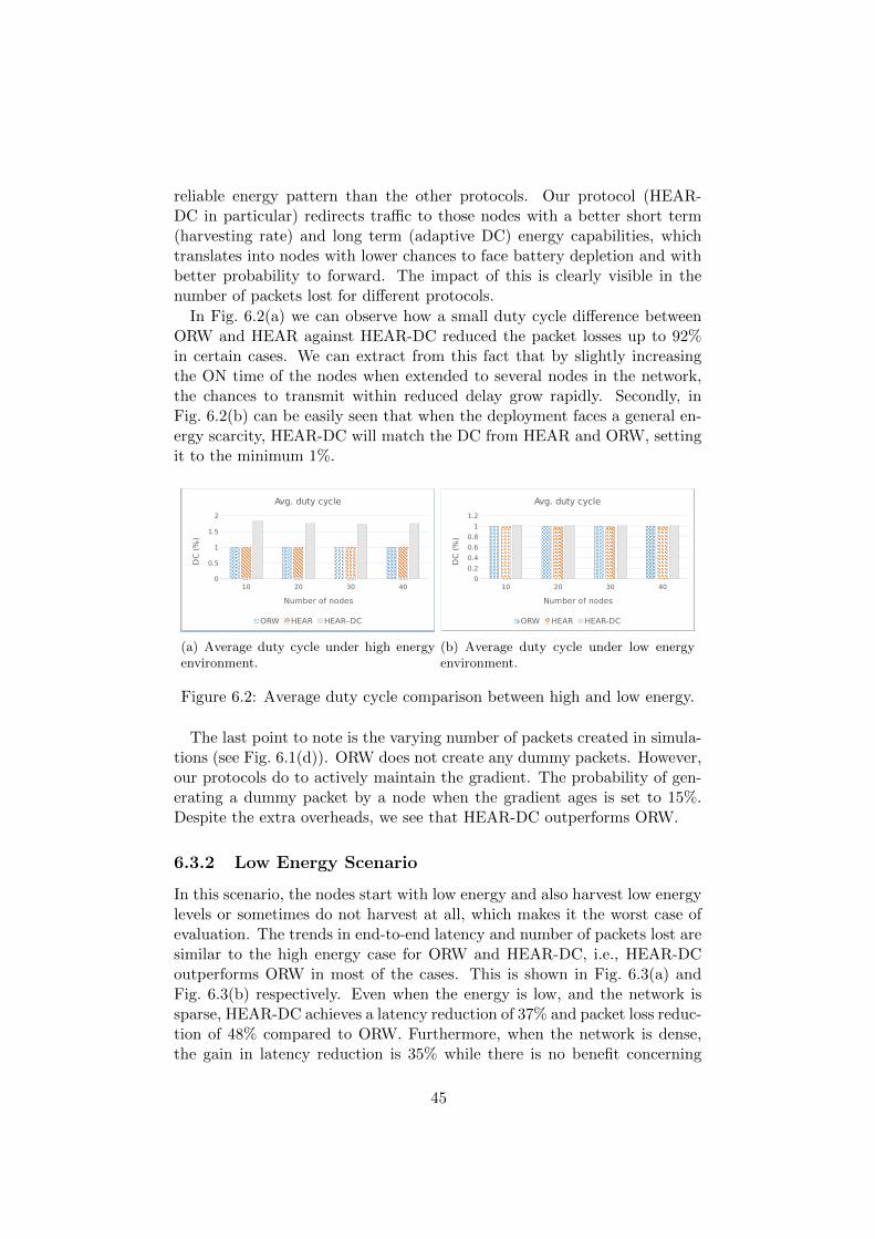
reliable energy pattern than the other protocols. Our protocol (HEAR-DC in particular) redirects traffic to those nodes with a better short term(harvesting rate) and long term (adaptive DC) energy capabilities, whichtranslates into nodes with lower chances to face battery depletion and withbetter probability to forward. The impact of this is clearly visible in thenumber of packets lost for different protocols.

In Fig. 6.2(a) we can observe how a small duty cycle difference betweenORW and HEAR against HEAR-DC reduced the packet losses up to 92%in certain cases. We can extract from this fact that by slightly increasingthe ON time of the nodes when extended to several nodes in the network,the chances to transmit within reduced delay grow rapidly. Secondly, inFig. 6.2(b) can be easily seen that when the deployment faces a general en-ergy scarcity, HEAR-DC will match the DC from HEAR and ORW, settingit to the minimum 1%.

(a) Average duty cycle under high energyenvironment.

(b) Average duty cycle under low energyenvironment.

Figure 6.2: Average duty cycle comparison between high and low energy.

The last point to note is the varying number of packets created in simula-tions (see Fig. 6.1(d)). ORW does not create any dummy packets. However,our protocols do to actively maintain the gradient. The probability of gen-erating a dummy packet by a node when the gradient ages is set to 15%.Despite the extra overheads, we see that HEAR-DC outperforms ORW.

6.3.2 Low Energy Scenario

In this scenario, the nodes start with low energy and also harvest low energylevels or sometimes do not harvest at all, which makes it the worst case ofevaluation. The trends in end-to-end latency and number of packets lost aresimilar to the high energy case for ORW and HEAR-DC, i.e., HEAR-DCoutperforms ORW in most of the cases. This is shown in Fig. 6.3(a) andFig. 6.3(b) respectively. Even when the energy is low, and the network issparse, HEAR-DC achieves a latency reduction of 37% and packet loss reduc-tion of 48% compared to ORW. Furthermore, when the network is dense,the gain in latency reduction is 35% while there is no benefit concerning

45



Figure 6.3: Performance comparison depending on number of nodes de-ployed under low energy environment.

packet losses.

Another observation is that HEAR performs better than ORW in mostcases (comparable in the 20 node case as well). In the case of ORW, underthe low energy regime, it may select nodes with higher link quality andcloser to the sink (lower EDC), however, they may run out of energy leadingto a bad performance. With HEAR and HEAR-DC, the energy level isgiven a high preference in route selection, leading to lower delays and lowerpacket losses. The performance of HEAR saturates at 30 nodes, and a higherdensity does not result in better results. This is due to the limited DC ofthe nodes.

The number of hops is more for ORW as shown in Fig. 6.3(c). Thisoccurs due to the incorrect updates of EDC. Since many nodes die andcome up again, EDC of the nodes is no longer valid, which gets propagated.Furthermore, even the nodes alive will not have an updated EDC due toan outage of many neighboring nodes. These make packets take incorrectdeviations, leading to longer routes and higher packet losses.

The effects of our gradient together with adaptive DC can be seen in thisscenario. Fig. 6.3.2 presents the number of node death occurrences in thisscenario for various protocols. While this number is more or less the samefor all protocols, the performance as shown in Fig. 6.3 is much better.

46

Figure 6.4: Node death occurrences under low energy.

6.3.3 Protocol Evaluation under Variable Traffic

In this section, we examine the influence of traffic load variations over thesame fixed network, in this case, 20 nodes. We have five different packetgeneration patterns or intervals. First, we set all nodes to create packetsperiodically at various interval times. To avoid strict synchronization werandomized around the same mean the moment to generate the new data.Therefore, the resulting packet generation intervals fall around the followingvalues: E[15s], E[45s], E[90s], E[180s] and finally we test the differentprotocols under event trigger packet generation. In this last scenario, thenodes will only generate packets when they experience a change in theirharvesting rate beyond a certain threshold. In Fig. 6.5 we can observe thesame four parameters as the previous experiments - delay 6.5(a), packetslost 6.5(b), number of hops 6.5(c) and number of packets created 6.5(d).

The end-to-end latency decreases as fewer packets are generated for allprotocols. Similarly, the packet losses also reduce since the network ex-periences lower packet exchanges. We observe 17% lower end-to-end delayand 13% lower packet losses when the traffic is very high (15 s). However,as traffic decreases, the performance gap between ORW and HEAR-DC re-duces significantly. This is mostly due to nodes having more energy bufferedfrom harvesting. The most interesting case for evaluating our adaptationfor sparse data (Sec. 4.6.1) is sending packets when an event trigger occurs.Due to our adaptation, we see that the adaptation enforces to result in muchlower delay than ORW - all packets with HEAR-DC were delivered within5 s, whereas ORW required a minimum of 19 s. Since the metric in ORWgets outdated, it begins to take some deviations as can be seen in Fig. 6.5(c).

6.3.4 Impact of Mobile Nodes

Lastly, we examine the impact of adding mobile nodes in the network. Mo-bile nodes change position throughout the simulation duration. We simulatemobile nodes with a Cooja plugin named mobility. This plugin allows the

47



Figure 6.5: Performance comparison depending on traffic under averageenergy environment.

user to upload a path file that indicates at each simulation instance the po-sition of each node. The outcome of using such plugin appears as the nodes‘teleport’ from one location to another.

We designed three different test scenarios in which we vary the percentageof mobile nodes deployed in it. The network has a total of 30 nodes, withthe number of mobile nodes being from 5, 10, and 15 nodes across the threescenarios.

48



Figure 6.6: Performance comparison depending on mobile node percentageunder average energy environment.

In Fig. 6.6 we see the results from this set of simulations. We observe alittle difference between the protocols when the percentage of mobile nodesis 17%. A visible gain is seen in the case when 1/3 nodes are mobile -the end-to-end delays of HEAR and HEAR-DC are 45% and 53% better ascompared to ORW. However, the delays slightly increase since the numberof forwarding nodes reduces. This trend is more pronounced when half ofthe nodes are mobile. HEAR and HEAR-DC clearly outperform ORW inthis case too, since ORW does not choose the routes that are more ‘reliable’.

49

Chapter 7

Conclusions and FutureWork

7.1 Conclusions

With the proliferation of Internet of Things (IoTs), smart homes are justaround the corner. Particularly, Active and Assisted Living (AAL) forpeople in their daily life application is of importance due their benefits.Two important requirements in the AAL scenario: (i) the ability to beavailable, i.e., be operational for extended periods of time; and (ii) scal-able, i.e., be able to include more technologies (e.g., new on-body sensors)over time. We adopt a network architecture in which backbone nodes arestatically deployed, and the mobile nodes connect to any possible emplacednode for data transfer. To make the nodes operate perpetually, we look topower all the nodes through energy-harvesting. However, it is challengingto collect data reliably with energy variations across the network. It is moreso in indoor environments where the harvested energy levels are very small,typically in µJ.

To this end, we proposed a novel routing protocol HEAR-DC which ismade up of several components: (i) transmitter-initiated MAC with oppor-tunistic reception and duplicate avoidance; (ii) an energy-harvesting awaregradient; (iii) adaptive duty cycling; and (iv) adaptations to support mo-bile nodes and sparse data traffic. The philosophy of this protocol is toopportunistic use of available energy and wireless channel for routing.

We developed a trace-based energy-harvesting simulation module for Cooja,which did not exist hitherto. We discussed the design, implementation, andlimitations of this module. Using the same module, we evaluated our pro-tocol against HEAR (HEAR-DC but with fixed duty cycle) and state-of-the-art opportunistic routing protocol, ORW. In the best case, i.e., when theenergy levels are high, and the harvesting rates are high, we found with 10nodes, HEAR-DC achieved a latency reduction of 64% with 92.75% lower

51

packet losses compared to ORW. With a higher density of nodes, perform-ance gains were lower. In the worst case, i.e., when the energy levels arelow, and the harvesting rates are low, with 10 nodes HEAR-DC achieveda substantial latency reduction of 37% and packet loss reduction of 48%compared to ORW. Due to the adaptation for sparse data traffic, the delayintroduced by HEAR-DC is almost by a factor of four lower than ORW whenonly event-triggers were sent. Furthermore, with more than half of the net-work having mobile nodes that are only data sources, HEAR-DC achieved31% lower delay and 46% lower packet loss with respect to ORW.

We observed that HEAR-DC outperforms both HEAR and ORW in allcases. HEAR outperforms ORW only in the cases when energy is aroundthe critical mark with several nodes on the verge of outage or dead. This isclearly because ORW does not consider energy variations into account. Wedraw this and other inferences from the results from all scenarios.

1. ORW does not adapt to the energy conditions well but works as goodas HEAR-DC when the density of the nodes is high enough. However,its performance does not significantly improve if the density is keptbut energy harvesting opportunities are increased. The limitation ismainly due to the fixed 1% duty cycle. Adding adaptive DC to ORWwill work well in the high energy scenario but also fail in the low energyscenario since there is little room for adaptive DC to perform. Theinference is ORW, as is set by default, is not suited for EH-WSNs.

2. HEAR, on the other hand, performs badly when the energy input ishigh on the network since high energy nodes attract a lot of packets,but will fail to deliver them due to a fixed duty cycle of 1%. HEARperforms relatively better than ORW in the low energy case simplybecause the packets get queued in the high energy nodes, which havea high chance of reliable delivery. The conclusion is that energy har-vesting aware gradient is important, but is not sufficient to offer goodperformance.

3. HEAR-DC outperforms all other protocols. Since HEAR-DC is a com-bination of our gradient and adaptive DC, we are interested to findout which one has more effect on the results. We see the performanceof gradient only in HEAR, which works well when adaptive DC haslittle role to play. Only adaptive DC in this case would result in a badperformance. However, when the energy in the buffer is even slightlyabove the set-point, the adaptive DC makes a huge difference withrespect to our metrics of delay and packet losses. In an average casescenario, both adaptive DC and gradient will work in synergy to offerbetter performance.

4. Most AAL networks will have low traffic and most probably an event-triggered sensing mechanism. As shown before, with ORW we will

52

have to endure a lot of delays due to aging, while our adaptation ofdummy packets offers lower delay. The tradeoff between energy spentfor dummy packet and delay for actual data packets is acceptable asthe harvested energy, if unused, is useless.

5. While HEAR-DC works the best among the protocols, in real de-ployment a critical density of nodes must be available to have a useracceptable performance.

7.2 Future Work

There are several extensions that are needed to this work. The most criticalone is to compare this work with ORiNoCo, which is a protocol adapted forEH-WSNs. Although we implemented it, we could not sort out all the bugswithin the time-frame of the thesis.

The next step would then be to evaluate the protocols on a real testbed.While Cooja has the multipath radio model, it is only a simple model ofthe reality of harsh wireless network. Collisions and packet losses can affectthe protocols significantly. Furthermore, this scenario would give us anopportunity to test if link-quality component of ORW will make a significantdifference with respect to our gradient.

Several limitations and questions were raised in the context of our trace-based simulation module. These restrictions must be addressed to enablebetter evaluation of all EH-WSN protocols.

53

Bibliography

[1] 200 hours of accelerometer information recorded over 25 days from5 participants. Columbia University. url: http://crawdad.org/

columbia/kinetic/20140513/.

[2] AAL European Union. url: http : / / www . aal - europe . eu / wp -

content/uploads/2015/11/20151001-AAL-Strategy_Final.pdf.

[3] H. D. AkaydIn, N. Elvin and Y. Andreopoulos. “Wake of a cylinder:A paradigm for energy harvesting with piezoelectric materials”. In:Experiments in Fluids 49.1 (2010), pp. 291–304. issn: 07234864. doi:10.1007/s00348-010-0871-7.

[4] David Benedetti, Chiara Petrioli and Dora Spenza. “GreenCastalia:an energy-harvesting-enabled framework for the castalia simulator”.In: Proceedings of the 1st International Workshop on Energy NeutralSensing Systems. ACM. 2013, p. 7.

[5] Alessandro Bogliolo, Emanuele Lattanzi and Andrea Acquaviva. “En-ergetic sustainability of environmentally powered wireless sensor net-works”. In: Proceedings of the 3rd ACM international workshop onPerformance evaluation of wireless ad hoc, sensor and ubiquitous net-works - PE-WASUN ’06 (2006), p. 149. doi: 10.1145/1163610.

1163636. url: http : / / portal . acm . org / citation . cfm ? doid =

1163610.1163636.

[6] Max Braun. “My Bathroom Mirror Is Smarter Than Yours”. In: (2016).url: https://medium.com/@maxbraun/my-bathroom-mirror-is-smarter-than-yours-94b21c6671ba#.gh6hzxanp.

[7] Renner Christian. “Perpetual Data Collection with Energy-HarvestingSensor Networks”. In: ACM Transactions on Sensor Networks 11.1(2014). issn: 15504859. doi: 10.1145/2566675.

[8] Mina Cong et al. CRAWDAD dataset columbia/kinetic (v. 2014-05-13). Downloaded from http://crawdad.org/columbia/kinetic/20140513/kinetic-energy. traceset: kinetic-energy. May 2014. doi: 10.15783/C73W29.

[9] Contiki Development at ANRG, University of Southern California.Contiki Netstack. url: http://anrg.usc.edu/contiki/index.php/Network_Stack.

55

http://crawdad.org/columbia/kinetic/20140513/

http://crawdad.org/columbia/kinetic/20140513/

http://www.aal-europe.eu/wp-content/uploads/2015/11/20151001-AAL-Strategy_Final.pdf

http://www.aal-europe.eu/wp-content/uploads/2015/11/20151001-AAL-Strategy_Final.pdf

http://dx.doi.org/10.1007/s00348-010-0871-7

http://dx.doi.org/10.1145/1163610.1163636

http://dx.doi.org/10.1145/1163610.1163636

http://portal.acm.org/citation.cfm?doid=1163610.1163636

http://portal.acm.org/citation.cfm?doid=1163610.1163636

https://medium.com/@maxbraun/my-bathroom-mirror-is-smarter-than-yours-94b21c6671ba#.gh6hzxanp

https://medium.com/@maxbraun/my-bathroom-mirror-is-smarter-than-yours-94b21c6671ba#.gh6hzxanp

http://dx.doi.org/10.1145/2566675

http://dx.doi.org/10.15783/C73W29

http://anrg.usc.edu/contiki/index.php/Network_Stack

http://anrg.usc.edu/contiki/index.php/Network_Stack

[10] Cooperative Networks For Renewable Resource Measurements. SolarEnergy Resource Data. url: http://rredc.nrel.gov/solar/new_data/confrrm/.

[11] Dataset of radiant light energy measurements. Columbia University.url: http://crawdad.org/columbia/enhants/20110407/.

[12] D. Dondi et al. “Modeling and Optimization of a Solar Energy Har-vester System for Self-Powered Wireless Sensor Networks”. In: IEEETransactions on Industrial Electronics 55.7 (2008), pp. 2759–2766.issn: 0278-0046. doi: 10.1109/TIE.2008.924449.

[13] Guangcheng Dong et al. “Thermal fatigue behaviour of Al¡DN¿2¡/DN¿O¡DN¿3¡/DN¿-DBC substrates under high temperature cyclic loading”. In: Soldering& Surface Mount Technology 22.November 2009 (2010), pp. 43–48.issn: 0954-0911. doi: 10.1108/09540911011036280.

[14] Euhanna Ghadimi and O Landsiedel. “Opportunistic Routing in LowDuty-Cycled Wireless Sensor Networks”. In: ACM Transactions onSensor Networks (2014). doi: 10.1145/0000000.0000000. url: https://people.kth.se/%7B~%7Deuhanna/pub/oppTOSN.pdf.

[15] Omprakash Gnawali et al. “Collection tree protocol”. In: Proceedingsof the 7th ACM conference on embedded networked sensor systems.ACM. 2009, pp. 1–14.

[16] Maria Gorlatova et al. CRAWDAD dataset columbia/enhants (v. 2011-04-07). Downloaded from http://crawdad.org/columbia/enhants/20110407/energy.traceset: energy. Apr. 2011. doi: 10.15783/C77P47.

[17] Maria Gorlatova et al. “Movers and Shakers: Kinetic Energy Harvest-ing for the Internet of Things”. In: (2013), p. 15. doi: 10 . 1145 /

2591971.2591986. arXiv: 1307.0044. url: http://arxiv.org/abs/1307.0044.

[18] Maria Gorlatova et al. “Movers and shakers: Kinetic energy harvest-ing for the internet of things”. In: ACM SIGMETRICS PerformanceEvaluation Review. Vol. 42. 1. ACM. 2014, pp. 407–419.

[19] David Hasenfratz et al. “Analysis, comparison, and optimization ofrouting protocols for energy harvesting wireless sensor networks”. In:Sensor Networks, Ubiquitous, and Trustworthy Computing (SUTC),2010 IEEE International Conference on. IEEE. 2010, pp. 19–26.

[20] Aman Kansal et al. “Power management in energy harvesting sensornetworks”. In: ACM Transactions on Embedded Computing Systems(TECS) 6.4 (2007), p. 32.

[21] K Kaushik et al. “Experimental Demonstration of Multi-Hop RF En-ergy Transfer”. In: International Symposium on Personal, Indoor andMobile Radio Communications (2013), pp. 538–542.

56

http://rredc.nrel.gov/solar/new_data/confrrm/

http://rredc.nrel.gov/solar/new_data/confrrm/

http://crawdad.org/columbia/enhants/20110407/

http://dx.doi.org/10.1109/TIE.2008.924449

http://dx.doi.org/10.1108/09540911011036280

http://dx.doi.org/10.1145/0000000.0000000

https://people.kth.se/%7B~%7Deuhanna/pub/oppTOSN.pdf

https://people.kth.se/%7B~%7Deuhanna/pub/oppTOSN.pdf

http://dx.doi.org/10.15783/C77P47

http://dx.doi.org/10.1145/2591971.2591986

http://dx.doi.org/10.1145/2591971.2591986

http://arxiv.org/abs/1307.0044



[22] Panqanamala Ramana Kumar and Pravin Varaiya. Stochastic systems:Estimation, identification, and adaptive control. Vol. 75. SIAM, 2015.

[23] Emanuele Lattanzi et al. “Energetic sustainability of routing algorithmsfor energy-harvesting wireless sensor networks”. In: Computer Com-munications 30.14-15 (2007), pp. 2976–2986. issn: 01403664. doi: 10.1016/j.comcom.2007.05.035.

[24] Sanghyo Lee et al. “Triboelectric energy harvester based on wearabletextile platforms employing various surface morphologies”. In: NanoEnergy 12 (2015), pp. 410–418.

[25] Longbi Lin, Ness B. Shroff and R. Srikant. “Asymptotically optimalenergy-aware routing for multihop wireless networks with renewableenergy sources”. In: IEEE/ACM Transactions on Networking 15.5(2007), pp. 1021–1034. issn: 10636692. doi: 10.1109/TNET.2007.896173.

[26] Paul D. Mitcheson et al. “Energy harvesting from human and machinemotion for wireless electronic devices”. In: Proceedings of the IEEE96.9 (2008), pp. 1457–1486. issn: 00189219. doi: 10.1109/JPROC.

2008.927494.

[27] David Moss and Philip Levis. “BoX-MACs: Exploiting physical andlink layer boundaries in low-power networking”. In: Computer SystemsLaboratory Stanford University (2008), pp. 116–119.

[28] Nikolaos A Pantazis, Stefanos A Nikolidakis and Dimitrios D Ver-gados. “Energy-efficient routing protocols in wireless sensor networks:A survey”. In: IEEE Communications Surveys & Tutorials 15.2 (2013),pp. 551–591.

[29] R. Venkatesha Prasad et al. “Reincarnation in the Ambiance: Devicesand networks with energy harvesting”. In: IEEE Communications Sur-veys and Tutorials 16.1 (2014), pp. 195–213. issn: 1553877X. doi:10.1109/SURV.2013.062613.00235.

[30] Mohammed Rahimi et al. “Studying the feasibility of energy harvest-ing in a mobile sensor network”. In: Robotics and Automation, 2003.Proceedings. ICRA’03. IEEE International Conference on. Vol. 1. IEEE.2003, pp. 19–24.

[31] Vijay S Rao et al. “On systems generating context triggers throughenergy harvesting”. In: IEEE Communications Magazine 52.6 (2014),pp. 70–77.

[32] Silvia Santini and Kay Romer. “An adaptive strategy for quality-baseddata reduction in wireless sensor networks”. In: Proceedings of the 3rdinternational conference on networked sensing systems (INSS 2006).2006, pp. 29–36.

57

http://dx.doi.org/10.1016/j.comcom.2007.05.035

http://dx.doi.org/10.1016/j.comcom.2007.05.035

http://dx.doi.org/10.1109/TNET.2007.896173

http://dx.doi.org/10.1109/TNET.2007.896173

http://dx.doi.org/10.1109/JPROC.2008.927494

http://dx.doi.org/10.1109/JPROC.2008.927494

http://dx.doi.org/10.1109/SURV.2013.062613.00235

[33] SeeedStudio [online]. url: http://seeedstudio.com.

[34] Nathan S Shenck and Joseph A Paradiso. “Energy scavenging withshoe-mounted piezoelectrics”. In: IEEE micro 21.3 (2001), pp. 30–42.

[35] Tmote Sky. “Ultra low power IEEE 802.15. 4 compliant wireless sensormodule”. In: Moteiv Corporation (2006).

[36] Tmote Sky datasheet. url: http://www.eecs.harvard.edu/~konrad/projects/shimmer/references/tmote-sky-datasheet.pdf.

[37] Stefan Untersch, Christian Renner and Volker Turau. “Data-CollectionProtocol”. In: (2012), pp. 1–16.

[38] Christopher M Vigorito, Deepak Ganesan and Andrew G Barto. “Ad-aptive control of duty cycling in energy-harvesting wireless sensor net-works”. In: 2007 4th Annual IEEE Communications Society Confer-ence on Sensor, Mesh and Ad Hoc Communications and Networks.IEEE. 2007, pp. 21–30.

[39] Anthony Wood et al. “Alarm-net: Wireless sensor networks for assisted-living and residential monitoring”. In: University of Virginia ComputerScience Department Technical Report 2 (2006).

[40] Jingjing Zhao and Zheng You. “A shoe-embedded piezoelectric energyharvester for wearable sensors”. In: Sensors 14.7 (2014), pp. 12497–12510.

[41] Linfeng Zheng et al. “Novel methods for estimating lithium-ion batterystate of energy and maximum available energy”. In: Applied Energy178 (2016), pp. 1–8.

58

http://seeedstudio.com

http://www.eecs.harvard.edu/~konrad/projects/shimmer/references/tmote-sky-datasheet.pdf

http://www.eecs.harvard.edu/~konrad/projects/shimmer/references/tmote-sky-datasheet.pdf

opportunistic routing for indoor energy harvesting wireless sensor networks · ·...

Documents