operational modal analysis of civil engineering structures || mathematical tools for random data...

Mathematical Tools for RandomData Analysis 2

2.1 Complex Numbers, Euler’s Identities,and Fourier Transform

Sinusoidal signals are frequently used in signal processing and system analysis.

In fact, sines and cosines are orthogonal functions and form a base for the analysis

of signals. Moreover, they are eigenfunctions for LTI systems. However, in order to

simplify operations and mathematical manipulations, sinusoidal signals are often

expressed by complex numbers and exponential functions.

Consider a sinusoidal function characterized by amplitude M> 0, frequency ωand phase angle φ:

y tð Þ ¼ M cos ω � t� φð Þ ð2:1ÞTaking advantage of the Euler’s formulas:

eiX ¼ cos Xð Þ þ i � sin Xð Þ ð2:2Þ

e�iX ¼ cos Xð Þ � i � sin Xð Þ ð2:3Þ

cos Xð Þ ¼ eiX þ e�iX

2ð2:4Þ

sin Xð Þ ¼ eiX � e�iX

2ið2:5Þ

where i is the imaginary unit (i2¼�1), y(t) can be rewritten in terms of complex

exponentials:

y tð Þ ¼ M

2ei ω�t�φð Þ þM

2e�i ω�t�φð Þ ð2:6Þ

C. Rainieri and G. Fabbrocino, Operational Modal Analysis of Civil EngineeringStructures: An Introduction and Guide for Applications, DOI 10.1007/978-1-4939-0767-0_2,# Springer Science+Business Media New York 2014

23

The representation in terms of complex numbers and exponential functions has

several advantages. First of all, the representation in terms of exponential functions

simplifies computations and analytical derivations. In fact, they convert product

into sum (2.7) and power into product (2.8), and the derivative of an exponential

function is the function itself multiplied by a factor (2.9).

ea � eb ¼ eaþb ð2:7Þ

eað Þb ¼ ea�b ð2:8Þd eað Þdb

¼ da

dbea ð2:9Þ

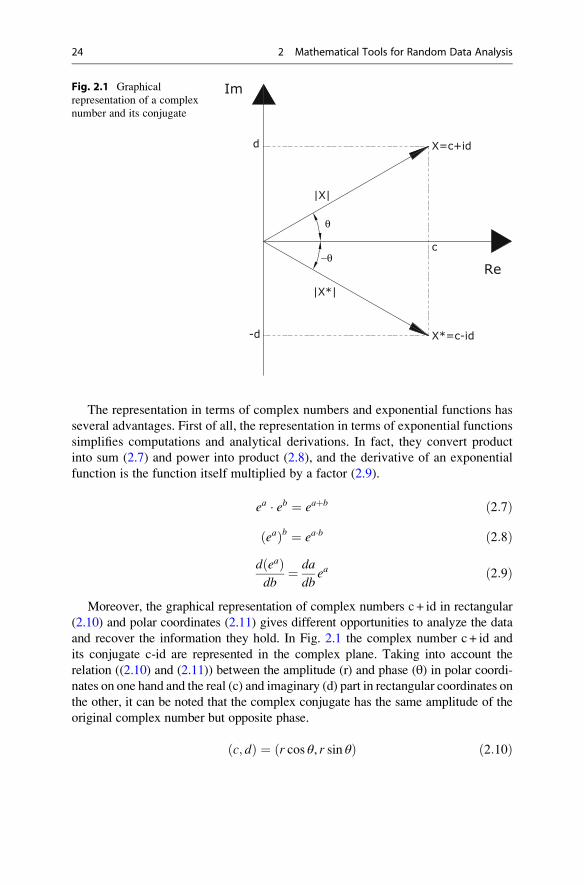
Moreover, the graphical representation of complex numbers c + id in rectangular

(2.10) and polar coordinates (2.11) gives different opportunities to analyze the data

and recover the information they hold. In Fig. 2.1 the complex number c + id and

its conjugate c-id are represented in the complex plane. Taking into account the

relation ((2.10) and (2.11)) between the amplitude (r) and phase (θ) in polar coordi-

nates on one hand and the real (c) and imaginary (d) part in rectangular coordinates on

the other, it can be noted that the complex conjugate has the same amplitude of the

original complex number but opposite phase.

c; dð Þ ¼ r cos θ, r sin θð Þ ð2:10Þ

Re

Im

c

d

-d

X=c+id

X*=c-id

|X|

|X*|

θ

−θ

Fig. 2.1 Graphical

representation of a complex

number and its conjugate

24 2 Mathematical Tools for Random Data Analysis

r; θð Þ ¼ffiffiffiffiffiffiffiffiffiffiffiffiffiffiffic2 þ d2

p, arctan

d

c

� �ð2:11Þ

On the other hand, algebraic operations with complex numbers lead to

operations with real numbers taking into account that i2¼�1, treating complex

number as polynomials and multiplying numerator and denominator by the com-

plex conjugate of the denominator in the division:

cþ idð Þ þ eþ ifð Þ ¼ cþ eð Þ þ i d þ fð Þ ð2:12Þcþ idð Þ � eþ ifð Þ ¼ c � e� d � fð Þ þ i c � f þ d � eð Þ ð2:13Þcþ idð Þeþ ifð Þ ¼

cþ idð Þ e� ifð Þeþ ifð Þ e� ifð Þ ¼

cþ idð Þ e� ifð Þe2 þ f 2

ð2:14Þ

Operations with complex numbers satisfy the commutative, associative, and

distributive rules.

The idea behind the Fourier analysis is that any signal can be decomposed as a

linear combination of sinusoidal functions at different frequencies. This can be

understood by taking into account the relation between sinusoidal functions and

complex exponentials and that both are orthogonal functions, that is to say, they

fulfill the following general conditions ((2.15) and (2.16)):

ð b

a

f u tð Þf �v tð Þdt ¼ 0, u 6¼ v ð2:15Þð b

a

f u tð Þf �v tð Þdt 6¼ 0 < 1, u ¼ v ð2:16Þ

where fu and fv are complex valued functions and the superscript * means complex

conjugate. In particular, this type of decomposition, originally developed for

periodical functions, can be extended to nonperiodic functions, such as transients

and random signals, by assuming that they are periodic functions with period equal

to the duration T of the signal. For a nonperiodic signal x(t), the (forward) Fourier

transform (analysis equation: (2.17)) and the inverse Fourier transform (synthesisequation: (2.18)) are given by:

X fð Þ ¼ðþ1

�1x tð Þe�i2πftdt ð2:17Þ

x tð Þ ¼ðþ1

�1X fð Þei2πftdf : ð2:18Þ

Thus, (2.17) shows that any signal x(t) can be decomposed in a sum (represented

by the integral) of sinusoidal functions (recall the Euler’s formula relating complex

exponentials and sinusoidal functions, (2.2) and (2.3)). In practical applications,

2.1 Complex Numbers, Euler’s Identities, and Fourier Transform 25

when the signal x(t) is recorded and analyzed by means of digital equipment, it is

represented by a sequence of values at discrete equidistant time instants. As a

consequence, only discrete time and frequency representations are considered,

and the expression of the Fourier transform has to be changed accordingly.

First of all, when dealing with discrete signals it is worth noting that the

sampling interval Δt is the inverse of the sampling frequency fs (representing the

rate by which the analog signal is sampled and digitized):

Δt ¼ 1

f s: ð2:19Þ

In order to properly resolve the signal, fs has to be selected so that it is at least twice

the highest frequency fmax in the time signal:

f s � 2fmax: ð2:20ÞMoreover, the following “uncertainty principle” holds:

Δf ¼ 1

NΔtð2:21Þ

In the presence of a finite number N of samples, the frequency resolution Δf canonly be improved at the expense of the resolution in time Δt, and vice versa. As a

consequence, for a given sampling frequency, a small frequency spacing Δf is

always the result of a long measuring time T (large number of samples N):

T ¼ NΔt ð2:22ÞAssuming that the signal x(t) has been sampled at N equally spaced time instants

and that the time spacing Δt has been properly selected (it satisfies the Shannon’s

theorem (2.20)), the obtained discrete signal is given by:

xn ¼ x nΔtð Þ n ¼ 0, 1, 2, . . . ,N � 1: ð2:23ÞTaking into account the uncertainty principle expressed by (2.21), the discrete

frequency values for the computation of X(f) are given by:

f k ¼k

T¼ k

NΔtk ¼ 0, 1, 2, . . . ,N � 1 ð2:24Þ

and the Fourier coefficients at these discrete frequencies are given by:

Xk ¼XN�1

n¼0

xne�i2 πkn

N k ¼ 0, 1, 2, . . . ,N � 1: ð2:25Þ


The Xk coefficients are complex numbers and the function defined in (2.25) is

often referred to as the Discrete Fourier Transform (DFT). Its evaluation requires

N2 operations. As a consequence, in an attempt to reduce the number of operations,

the Fast Fourier Transform (FFT) algorithm has been developed (Cooley and

Tukey 1965). Provided that the number of data points equals a power of 2, the

number of operations is reduced to N · log2N. The inverse DFT is given by:

xn ¼ 1

N

XN�1

k¼0

Xkei2πknN n ¼ 0, 1, 2, . . . ,N � 1 ð2:26Þ

The coefficient X0 captures the static component of the signal (DC offset).

The magnitude of the Fourier coefficient Xk relates to the magnitude of the sinusoid

of frequency fk that is contained in the signal with phase θk:

Xkj j ¼ffiffiffiffiffiffiffiffiffiffiffiffiffiffiffiffiffiffiffiffiffiffiffiffiffiffiffiffiffiffiffiffiffiffiffiffiffiffiffiffiffiffiffiRe Xkð Þ½ �2 þ Im Xkð Þ½ �2

qð2:27Þ

θk ¼ arctanIm Xkð ÞRe Xkð Þ

� �ð2:28Þ

The Fourier transform is a fundamental tool in signal analysis, and it has the

following important properties:

• Linearity: given two discrete signals x(t) and y(t), the Fourier transform of any

linear combination of the signals is given by the same linear combination of the

transformed signals X(f) and Y(f);

• Time shift: if X(f) is the Fourier transform of x(t), thenX fð Þe�i2πf t0 is the Fourier

transform of x(t-t0);

• Integration and differentiation: integrating in the time domain corresponds to

dividing by i2πf in the frequency domain, differentiating in the time domain to

multiplying by i2πf in the frequency domain;

• Convolution: convolution in time domain corresponds to a multiplication in the

frequency domain, and vice versa; for instance, the Fourier transform of the

following convolution integral:

a tð Þ ¼ðþ1

�1b τð Þ � c t� τð Þdτ ¼ b tð Þ∗c tð Þ ð2:29Þ

is given by:

A fð Þ ¼ B fð Þ � C fð Þ ð2:30ÞThese last two properties are some of the major reasons for the extensive use of

the Fourier transform in signal processing, since complex calculations are

transformed into simple multiplications.

2.1 Complex Numbers, Euler’s Identities, and Fourier Transform 27

2.2 Stationary Random Data and Processes

2.2.1 Basic Concepts

The observed data representing a physical phenomenon can sometimes be

described by an explicit mathematical relationship: in such a case, data are deter-

ministic. The observed free vibration response of a SDOF system under a set of

initial conditions is an example of deterministic data, since it is governed by an

explicit mathematical expression depending on the mass and stiffness properties of

the system. On the contrary, random data cannot be described by explicit mathe-

matical relationships (the exact value at a certain time instant cannot be predicted)

and they must be described in probabilistic terms.

A random (or stochastic) process is the collection of all possible physical

realizations of the random phenomenon. A sample function is a single time history

representing the random phenomenon and, as such, is one of its physical realiza-

tions. A sample record is a sample function observed over a finite time interval; as

such, it can be thought as the observed result of a single experiment. In the

following, attention is focused on Stationary Random Processes (SRP) and, above

all, on the particular category of Stationary and Ergodic Random Processes (SERP).

A collection of sample functions (also called ensemble) is needed to characterizea random process. Said xk(t) the k-th function in the ensemble, at a certain time

instant t the mean value of the random process can be computed from the instanta-

neous values of each function in the ensemble at that time as follows:

μx tð Þ ¼ limK!1

1

K

XKk¼1

xk tð Þ: ð2:31Þ

In a similar way the autocorrelation function can be computed by taking

the ensemble average of the product of instantaneous values at time instants t andtþ τ:

Rxx t, tþ τð Þ ¼ limK!1

1

K

XKk¼1

xk tð Þxk tþ τð Þ: ð2:32Þ

Whenever the quantities expressed by (2.31) and (2.32) do not vary when the

considered time instant t varies, the random process is said to be (weakly)

stationary. For weakly stationary random processes, the mean value is independent

of the time t and the autocorrelation depends only on the time lag τ:

μx tð Þ ¼ μx ð2:33ÞRxx t, tþ τð Þ ¼ Rxx τð Þ: ð2:34Þ

In the following sections the basic descriptive properties for stationary random

records (probability density functions, auto- and cross-correlation functions, auto-

and cross-spectral density functions, coherence functions) are briefly discussed,


focusing the attention in particular on ergodic processes. The above-mentioned

descriptive properties are, in fact, primary tools of signal analysis. They are

commonly used to prepare the data for most OMA techniques.

2.2.2 Fundamental Notions of Probability Theory

A preliminary classification of data is based on their probability density function.

For a given random variable x, the random outcome of the k-th experiment is a

real number and it can be indicated as xk. The probability distribution functionP(x) provides, for any given value x, the probability that the k-th realization of the

random variable is not larger than x:

P xð Þ ¼ prob xk � x½ � ð2:35ÞMoreover, whenever the random variable assumes a continuous range of values,

the probability density function is defined as follows:

p xð Þ ¼ limΔx!0

prob x < xk � xþ Δx½ �Δx

ð2:36Þ

The probability density function and the probability distribution function show

the following properties:

p xð Þ � 0 ð2:37Þðþ1

�1p xð Þdx ¼ 1 ð2:38Þ

P xð Þ ¼ð x

�1p ζð Þdζ ð2:39Þ

P að Þ � P bð Þ if a � b ð2:40Þ

P �1ð Þ ¼ 0, P þ1ð Þ ¼ 1 ð2:41ÞIn a similar way, in the presence of two random variables x and y, it is possible to

define the joint probability distribution function:

P x; yð Þ ¼ prob xk � x and yk � y½ � ð2:42Þand the joint probability density function:

p xð Þ ¼ limΔx ! 0

Δy ! 0

prob x < xk � xþ Δx and y < yk � yþ Δy½ �ΔxΔy

ð2:43Þ

2.2 Stationary Random Data and Processes 29

The probability density functions of the individual random variables can be

obtained from the joint probability density function as follows:

p xð Þ ¼ðþ1

�1p x; yð Þdy ð2:44Þ

p yð Þ ¼ðþ1

�1p x; yð Þdx ð2:45Þ

If the following condition holds:

p x; yð Þ ¼ p xð Þp yð Þ ð2:46Þthe two random variables are statistically independent; for statistically independentvariables it also follows that:

P x; yð Þ ¼ P xð ÞP yð Þ ð2:47ÞWhen a random variable assumes values in the range (�1, +1), its mean value

(or expected value) can be computed from the product of each value with its

probability of occurrence as follows:

E xk½ � ¼ðþ1

�1xp xð Þdx ¼ μx: ð2:48Þ

In a similar way it is possible to define the mean square value as:

E x2k� � ¼

ðþ1

�1x2p xð Þdx ¼ ψ2

x ð2:49Þ

and the variance:

E xk � μxð Þ2h i

¼ðþ1

�1x� μxð Þ2p xð Þdx ¼ ψ2

x � μ2x ¼ σ2x : ð2:50Þ

By definition, the standard deviation σx is the positive square root of the

variance, and it is measured in the same units as the mean value.

The covariance function of two random variables is defined as:

Cxy ¼ E xk � μxð Þ yk � μy� �� ¼

ðþ1

�1

ðþ1

�1xk � μxð Þ yk � μy

� �p x; yð Þdxdy : ð2:51Þ

Taking into account that the following relation exists between the covariance of

the two random variables and their respective standard deviations:


Cxy

� σxσy ð2:52Þthe correlation coefficient can be defined as:

ρxy ¼Cxy

σxσy: ð2:53Þ

It assumes values in the range [�1, +1]. When it is zero, the two random variables

are uncorrelated. It is worth noting that, while independent random variables are also

uncorrelated, uncorrelated variables are not necessarily independent. However, it is

possible to show that, for physically important situations involving two or more

normally distributed random variables, being mutually uncorrelated does imply

independence (Bendat and Piersol 2000).

Relevant distributions for the analysis of data in view of modal identification are

the sine wave distribution and the Gaussian (or normal) distribution.

When a random variable follows a Gaussian distribution, its probability density

function is given by:

p xð Þ ¼ 1

σxffiffiffiffiffi2π

p e� x�μxð Þ2

2σ2x ð2:54Þ

while its probability distribution function is:

P xð Þ ¼ 1

σxffiffiffiffiffi2π

pð x

�1e� ζ�μxð Þ2

2σ2x dζ ð2:55Þ

with μx and σx denoting the mean value and the standard deviation of the random

variable, respectively. The Gaussian probability density and distribution functions

are often expressed in terms of the standardized variable z, characterized by zero

mean and unit variance:

z ¼ x� μxσx

ð2:56Þ

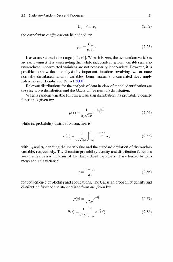
for convenience of plotting and applications. The Gaussian probability density and

distribution functions in standardized form are given by:

p zð Þ ¼ 1ffiffiffiffiffi2π

p e�z2

2 ð2:57Þ

P zð Þ ¼ 1ffiffiffiffiffi2π

pð x

�1e�

ζ2

2 dζ ð2:58Þ


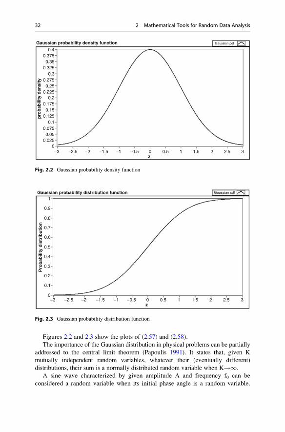
Figures 2.2 and 2.3 show the plots of (2.57) and (2.58).

The importance of the Gaussian distribution in physical problems can be partially

addressed to the central limit theorem (Papoulis 1991). It states that, given K

mutually independent random variables, whatever their (eventually different)

distributions, their sum is a normally distributed random variable when K!1.

A sine wave characterized by given amplitude A and frequency f0 can be

considered a random variable when its initial phase angle is a random variable.

Gaussian probability density function Gaussian pdfp

rob

abili

ty d

ensi

ty

0.40.3750.35

0.3250.3

0.2750.25

0.2250.2

0.1750.15

0.1250.1

0.0750.05

0.0250

−3 −2.5 −2 −1.5 −1 −0.5 0z

0.5 1 1.5 2 2.5 3

Fig. 2.2 Gaussian probability density function

Gaussian probability distribution function Gaussian cdf

1

0.9

0.8

0.7

0.6

0.5

0.4

0.3

0.2

0.1

0−3 −2.5 −2 −1.5 −1 −0.5 0

z0.5 1 1.5 2 2.5 3

Pro

bab

ility

dis

trib

uti

on

Fig. 2.3 Gaussian probability distribution function


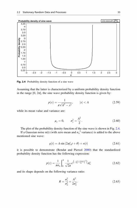
Assuming that the latter is characterized by a uniform probability density function

in the range [0, 2π], the sine wave probability density function is given by:

p xð Þ ¼ 1

πffiffiffiffiffiffiffiffiffiffiffiffiffiffiffiA2 � x2

p , xj j < A ð2:59Þ

while its mean value and variance are:

μx ¼ 0, σ2x ¼A2

2: ð2:60Þ

The plot of the probability density function of the sine wave is shown in Fig. 2.4.

If a Gaussian noise n(t) (with zero mean and σn2 variance) is added to the above

mentioned sine wave:

g tð Þ ¼ A sin 2πf 0tþ θð Þ þ n tð Þ ð2:61Þit is possible to demonstrate (Bendat and Piersol 2000) that the standardized

probability density function has the following expression:

p zð Þ ¼ 1

πσn

ð π

0

1ffiffiffiffiffi2π

p e �12

z�A cos ζσnð Þ2

� �dζ ð2:62Þ

and its shape depends on the following variance ratio:

R ¼ σ2sσ2n

¼ A2

2σ2n: ð2:63Þ

Probability density of sine wave4.25

3.753.5

3.253

2.752.5

2.252

1.751.5

1.251

0.750.5

0.25−3 −2.5 −2 −1.5 −1 −0.5 0

z

sine wave pdf

0.5 1.51 2 2.5 3

4

Pro

bab

ility

den

sity

Fig. 2.4 Probability density function of a sine wave


The estimation of probability density functions from recorded data and the

analysis of their shape provide an effective mean for the identification of spurious

harmonics superimposed to the stochastic response of the structure under test, as

shown in Chap. 5.

It is worth noting that, when dealing with finite records of the structural

response, an exact knowledge of parameters, such as mean and variance, and,

therefore, of probability density functions is generally not available. Only estimates

based on finite datasets can be obtained. Thus, it is desirable to get high quality

estimates from the available data. They can be obtained through an opportune

choice of the estimator. Since different estimators exist for the same quantity, the

choice should be oriented towards estimators that are:

• Unbiased: the expected value of the estimator is equal to the parameter being

established;

• Efficient: the mean square error of the estimator is smaller than for other possible

estimators;

• Consistent: the estimator approaches the parameter under estimation with a

probability approaching unity as the sample size increases.

Thus, even if a different choice is possible, the unbiased estimators for the mean

and variance given by:

μ x ¼1

N

XNi¼1

xi ð2:64Þ

σ 2x ¼

1

N � 1

XNi¼1

xi � μ xð Þ2 ð2:65Þ

are adopted in the following; the hat (^) indicates that the quantities in (2.64)

and (2.65) are estimates of the true mean and variance based on a finite number

of samples.

The probability density function of a record can be estimated by dividing the full

range of data into a number of intervals characterized by the same (narrow) width.

For instance, assuming that [a, b] is the full range of data values, it can be divided

into K intervals characterized by the equal width W:

W ¼ b� a

Kð2:66Þ

Then, the number Nk of data values falling into the k-th interval [dk-1, dk]:

dk�1 ¼ aþ k � 1ð ÞW, dk ¼ aþ kW ð2:67Þprovide the following estimate of the probability density function:

p xð Þ ¼ Nk

NW: ð2:68Þ


http://dx.doi.org/10.1007/978-1-4939-0767-0_5

Note that the first interval includes all values not larger than a, while the last

interval includes all values strictly larger than b. Moreover:

XKþ1

k¼0

Nk ¼ N: ð2:69Þ

The output of this procedure can be represented in the form of a sequence of

sample probability density estimates in accordance with (2.68):

p k ¼Nk

N

� �K

b� a

� �k ¼ 1, 2, . . . ,K ð2:70Þ

Alternatively, it can be either represented in the form of a histogram, which is

simply the sequence of the values of Nk without changes, or expressed in terms of

the sample percentage Nk/N of data in each interval.

2.2.3 Correlation Functions

Correlation functions play a primary role in output-only modal identification.

In fact, under the assumption of stationary and random response of the structure,

the second-order statistics of the response carry all the physical information.

Given the sample functions xk(t) and yk(t) of two stationary random processes,

the mean values, independent of t, are given by:

μx ¼ E xk tð Þ� � ¼ðþ1

�1xp xð Þdx ð2:71Þ

μy ¼ E yk tð Þ� � ¼ðþ1

�1yp yð Þdy ð2:72Þ

in agreement with (2.48). The assumption of stationary random processes yields

covariance functions that are also independent of t:

Cxx τð Þ ¼ E xk tð Þ � μxð Þ xk tþ τð Þ � μxð Þh i

ð2:73Þ

Cyy τð Þ ¼ E yk tð Þ � μy� �

yk tþ τð Þ � μy� �h i

ð2:74Þ

Cxy τð Þ ¼ E xk tð Þ � μxð Þ yk tþ τð Þ � μy� �h i

ð2:75Þ

If the mean values are both equal to zero, the covariance functions coincide with

the correlation functions:

Rxx τð Þ ¼ E xk tð Þxk tþ τð Þ� � ð2:76Þ


Ryy τð Þ ¼ E yk tð Þyk tþ τð Þ� � ð2:77Þ

Rxy τð Þ ¼ E xk tð Þyk tþ τð Þ� �: ð2:78Þ

The quantities Rxx and Ryy are called auto-correlation functions of xk(t) and

yk(t), respectively; Rxy is called cross-correlation function between xk(t) and yk(t).

When the mean values are not zero, covariance functions and correlation

functions are related by the following equations:

Cxx τð Þ ¼ Rxx τð Þ � μ2x ð2:79Þ

Cyy τð Þ ¼ Ryy τð Þ � μ2y ð2:80Þ

Cxy τð Þ ¼ Rxy τð Þ � μxμy: ð2:81Þ

Taking into account that two stationary random processes are uncorrelated if

Cxy(τ)¼ 0 for all τ (2.53) and that this implies Rxy(τ)¼ μxμy for all τ (2.81), if μx orμy equals zero the two processes are uncorrelated when Rxy(τ)¼ 0 for all τ.

Taking into account that the cross-correlation function and the cross-covariance

function are bounded by the following inequalities:

Cxy τð Þ 2 � Cxx 0ð ÞCyy 0ð Þ ð2:82Þ

Rxy τð Þ 2 � Rxx 0ð ÞRyy 0ð Þ ð2:83Þand noting that:

Cxx τð Þj j � Cxx 0ð Þ ð2:84ÞRxx τð Þj j � Rxx 0ð Þ ð2:85Þ

it follows that the maximum values of the auto-correlation and auto-covariance

functions occur at τ¼ 0; they correspond to the mean square value and variance of

the data, respectively:

Rxx 0ð Þ ¼ E x2k tð Þ� �, Cxx 0ð Þ ¼ σ2x : ð2:86Þ

When the mean values and covariance (correlation) functions of the considered

stationary random processes can be directly computed by means of time averages

on an arbitrary pair of sample records instead of computing ensemble averages, the

two stationary random processes are said to be weakly ergodic. In other words, in

the presence of two ergodic processes, the statistical properties of weakly stationary

random processes can be determined from the analysis of a pair of sample records

only, without the need of collecting a large amount of data. As a consequence, in the


presence of two ergodic processes, the mean values of the individual sample

functions can be computed by a time average as follows:

μx kð Þ ¼ limT!1

1

T

ð T

0

xk tð Þdt ¼ μx ð2:87Þ

μy kð Þ ¼ limT!1

1

T

ð T

0

yk tð Þdt ¼ μy: ð2:88Þ

The index k denotes that the k-th sample function has been chosen for the

computation of the mean value: since the processes are ergodic, the results are

independent of this choice (μx(k)¼ μx, μy(k)¼ μy). It is worth pointing out that

the mean values are also independent of the time t.

In a similar way, auto- and cross-covariance functions can be computed directly

from the k-th sample function as follows:

Cxx τ; kð Þ ¼ limT!1

1

T

ð T

0

xk tð Þ � μx� �

xk tþ τð Þ � μx� �

dt ¼

¼ Rxx τ; kð Þ � μ2x

ð2:89Þ

Cyy τ; kð Þ ¼ limT!1

1

T

ð T

0

yk tð Þ � μy� �

yk tþ τð Þ � μy� �

dt ¼

¼ Ryy τ; kð Þ � μ2y

ð2:90Þ

Cxy τ; kð Þ ¼ limT!1

1

T

ð T

0

xk tð Þ � μx� �

yk tþ τð Þ � μy� �

dt ¼

¼ Rxy τ; kð Þ � μxμy

ð2:91Þ

and, the processes being ergodic, the results are independent of the chosen function

(Cxx(τ, k)¼Cxx(τ), Cyy(τ, k)¼Cyy(τ), Cxy(τ, k)¼Cxy(τ)).It is worth pointing out that only stationary random processes can be ergodic.

When a stationary process is also ergodic, the generic sample function is represen-

tative of all others so that the first- and second-order properties of the process can

be computed from an individual sample function by means of time averages.

With stationary and ergodic processes, the auto- and cross-correlation functions

are given by the following expressions:

Rxx τð Þ ¼ limT!1

1

T

ð T

0

x tð Þx tþ τð Þdt ð2:92Þ

Ryy τð Þ ¼ limT!1

1

T

ð T

0

y tð Þy tþ τð Þdt ð2:93Þ

Rxy τð Þ ¼ limT!1

1

T

ð T

0

x tð Þy tþ τð Þdt: ð2:94Þ


Ergodic random processes are definitely an important class of random processes.

Since the time-averaged mean value and correlation function are equal to the

ensemble-averaged mean and correlation function respectively, a single sample

function is sufficient to compute those quantities instead of a collection of sample

functions. In practical applications stationary random processes are usually ergodic.

From a general point of view, a random process is ergodic if the following sufficient

conditions are fulfilled:

• The random process is weakly stationary and the time averages μx(k) and

Cxx(τ, k) ((2.87) and (2.89)) are the same for all sample functions;

• The auto-covariance function fulfills the following condition:

1

T

ð T

�T

Cxx τð Þj jdτ ! 0 for T ! 1: ð2:95Þ

In practical applications, individual time history records are referred to as

stationary if the properties computed over short time intervals do not significantly

vary from one interval to the next. In other words, eventual variations are limited to

statistical sampling variations only. Since a sample record obtained from an ergodic

process is stationary, verification of stationarity of the individual records justifies

the assumption of stationarity and ergodicity for the random process from which the

sample record is obtained. Tests for stationarity of data (Bendat and Piersol 2000)

are advisable before processing.

From a sample record, the correlation function can be estimated either through

direct computation or by means of FFT procedures. The latter approach is faster than

the former but suffers some drawbacks related to the underlying periodic assumption

of the DFT. If the direct estimation of the autocorrelation is considered, it is given by:

R xx rΔtð Þ ¼ 1

N � r

XN�r

n¼1

xnxnþr r ¼ 0, 1, 2, . . . ,m ð2:96Þ

for a stationary record with zero mean (μ¼ 0) and uniformly sampled data at Δt.Thus, (2.96) provides an unbiased estimate of the auto-correlation function at

the time delay rΔt, where r is also called the lag number and m denotes the

maximum lag.

2.2.4 Spectral Density Functions

Given a pair of sample records xk(t) and yk(t) of finite duration T from stationary

random processes, their Fourier transforms (which exist as a consequence of the

finite duration of the signals) are:

Xk f ; Tð Þ ¼ð T

0

xk tð Þe�i2 π ftdt ð2:97Þ


Yk f ; Tð Þ ¼ð T

0

yk tð Þe�i2 π ftdt ð2:98Þ

and the two-sided auto- and cross-spectral density functions are defined as follows:

Sxx fð Þ ¼ limT!1

E1

TX�k f ; Tð ÞXk f ; Tð Þ

�ð2:99Þ

Syy fð Þ ¼ limT!1

E1

TY�k f ; Tð ÞYk f ; Tð Þ

�ð2:100Þ

Sxy fð Þ ¼ limT!1

E1

TX�k f ; Tð ÞYk f ; Tð Þ

�ð2:101Þ

where * denotes complex conjugate. Two-sided means that S(f) is defined for f inthe range (�1, +1); the expected value operation is working over the ensemble

index k. The one-sided auto- and cross-spectral density functions, with f varying in

the range (0, +1), are given by:

Gxx fð Þ ¼ 2Sxx fð Þ ¼ 2 limT!1

1

TE Xk f ; Tð Þj j2h i

0 < f < þ1 ð2:102Þ

Gyy fð Þ ¼ 2Syy fð Þ ¼ 2 limT!1

1

TE Yk f ; Tð Þj j2h i

0 < f < þ1 ð2:103Þ

Gxy fð Þ ¼ 2Sxy fð Þ ¼ 2 limT!1

1

TE X�

k f ; Tð ÞYk f ;Tð Þ� �0 < f < þ1 ð2:104Þ

The two-sided spectral density functions are more commonly adopted in

theoretical derivations and mathematical calculations, while the one-sided spectral

density functions are typically used in the applications. In particular, in practical

applications the one-sided spectral density functions are always the result of Fourier

transforms of records of finite length (T<1) and of averaging of a finite number of

ensemble elements.

Before analyzing the computation of PSDs in practice, it is interesting to note

that PSDs and correlation functions are Fourier transform pairs. Assuming that

mean values have been removed from the sample records and that the integrals of

the absolute values of the correlation functions are finite (this is always true for

finite record lengths), that is to say:

ðþ1

�1R τð Þj jdτ < 1 ð2:105Þ


the two-sided spectral density functions are the Fourier transforms of the

correlation functions:

Sxx fð Þ ¼ðþ1

�1Rxx τð Þe�i2 π f τdτ ð2:106Þ

Syy fð Þ ¼ðþ1

�1Ryy τð Þe�i2 π f τdτ ð2:107Þ

Sxy fð Þ ¼ðþ1

�1Rxy τð Þe�i2 π f τdτ ð2:108Þ

Equations (2.106)–(2.108) are also called the Wiener-Khinchin relations in

honor of the mathematicians that first proved that correlations and spectral densities

are Fourier transform pairs. The auto-spectral density functions are real-valued

functions, while the cross-spectral density functions are complex-valued. In terms

of one-sided spectral density functions, the correspondence with the correlation

functions is given by:

Gxx fð Þ ¼ 4

ð1

0

Rxx τð Þ cos 2π f τð Þdτ ð2:109Þ

Gyy fð Þ ¼ 4

ð1

0

Ryy τð Þ cos 2π f τð Þdτ ð2:110Þ

Gxy fð Þ ¼ 2

ðþ1

�1Rxy τð Þe�i2πf τdτ ¼ Cxy fð Þ � iQxy fð Þ ð2:111Þ

where Cxy(f) is called the coincident spectral density function (co-spectrum) and

Qxy(f) is the quadrature spectral density function (quad-spectrum). The one-sided

cross-spectral density function can be also expressed in complex polar notation as

follows:

Gxy fð Þ ¼ Gxy fð Þ e�iθxy fð Þ 0 < f < 1 ð2:112Þwhere the magnitude and phase are given by:

Gxy fð Þ ¼ ffiffiffiffiffiffiffiffiffiffiffiffiffiffiffiffiffiffiffiffiffiffiffiffiffiffiffiffiffiffiffiffiffiC2xy fð Þ þ Q2

xy fð Þq

ð2:113Þ

θxy fð Þ ¼ arctanQxy fð ÞCxy fð Þ : ð2:114Þ


Taking into account that the cross-spectral density function is bounded by the

cross-spectrum inequality:

Gxy fð Þ 2 � Gxx fð ÞGyy fð Þ ð2:115Þit is possible to define the coherence function as follows:

γ2xy fð Þ ¼ Gxy fð Þ 2Gxx fð ÞGyy fð Þ ¼

Sxy fð Þ 2Sxx fð ÞSyy fð Þ ð2:116Þ

where:

0 � γ2xy fð Þ � 1 8 f : ð2:117Þ

Note that the conversion from two-sided to one-sided spectral density functions

doubles the amplitude (jSxy( f )j ¼ jGxy( f )j/2) while preserving the phase.

It is worth pointing out two important properties of Gaussian random processes

for practical applications. First, it can be shown (Bendat and Piersol 2000) that if a

Gaussian process undergoes a linear transformation, the output is still a Gaussian

process. Moreover, given a sample record of an ergodic Gaussian random process

with zero mean, it can be shown (Bendat and Piersol 2000) that the Gaussian

probability density function p(x):

p xð Þ ¼ 1

σxffiffiffiffiffiffi2π

p e� x2

2 σ2x ð2:118Þ

is completely determined by the knowledge of the auto-spectral density function.

In fact, taking into account that (Bendat and Piersol 2000):

σ2x ¼ðþ1

�1x2p xð Þdx �

ð 1

0

Gxx fð Þdf , ð2:119Þ

Gxx(f) alone determines σx. As a consequence, spectral density functions (and their

Fourier transform pairs, the correlation functions) play a fundamental role in the

analysis of random data, since they contain the information of interest.

In practical applications, PSDs can be obtained by computing the correlation

functions first and then Fourier transforming them. This approach is known as the

Blackman-Tukey procedure. Another approach, known as theWelch procedure, is,instead, based on the direct computation of the FFT of the records and the estima-

tion of the PSDs in agreement with (2.102)–(2.104). The Welch procedure is less

computational demanding than the Blackman-Tukey method, but it requires some

operations on the signal in order to improve the quality of the estimates.

According to (2.102)–(2.104), the one-sided auto-spectral density function

can be estimated by dividing a record into nd contiguous segments, each of length

T¼NΔt, Fourier transforming each segment and then computing the auto-spectral


density through an ensemble averaging operation over the nd subsets of data as

follows:

G xx fð Þ ¼ 2

ndNΔt

Xndi¼1

Xi fð Þj j2: ð2:120Þ

The number of data values N in each segment is often called the block size for thecomputation of each FFT; it determines the frequency resolution of the resulting

estimates. The number of averages nd, instead, determines the random error of the

estimates, as discussed in Sect. 2.2.5.

Even if the direct computation via FFT of the spectral density function is

advantageous from a computational point of view, specific strategies are required

to eliminate the errors originating from the fact that the estimates are based on

records of finite length. A sample record x(t) can be interpreted as an unlimited

record v(t) multiplied by a rectangular time window u(t):

x tð Þ ¼ u tð Þv tð Þ u tð Þ ¼ 1 0 � t � T0 elsewhere

�: ð2:121Þ

As a consequence, the Fourier transform of x(t) is given by the convolution of

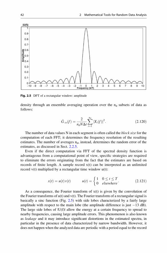
the Fourier transforms of u(t) and v(t). The Fourier transform of a rectangular signal is

basically a sinc function (Fig. 2.5) with side lobes characterized by a fairly large

amplitude with respect to the main lobe (the amplitude difference is just �13 dB).

The large side lobes of |U(f)| allow the energy at a certain frequency to spread to

nearby frequencies, causing large amplitude errors. This phenomenon is also known

as leakage and it may introduce significant distortions in the estimated spectra, in

particular in the presence of data characterized by narrow bandwidth. However, it

does not happen when the analyzed data are periodic with a period equal to the record

|U(f)|1

0.9

0.8

0.7

0.6

Am

plit

ud

e

0.5

0.4

0.3

0.2

0.1

0−10 −9 −8 −7 −6 −5 −4 −3 −2 −1 0

Frequency (k/T)1 2 3 4 5 6 7 8 9 10

Fig. 2.5 DFT of a rectangular window: amplitude


length. In such a case, in fact, the discrete frequency values, equally spaced at

Δf¼ 1/T, coincide with zeros of the spectral window in the frequency domain with

the only exception of the frequency line in the main lobe. The result is an exact

reproduction of the correct spectrum. Thus, in order to suppress the leakage problem,

data are made periodic by tapering them by an appropriate time window, which

eliminates the discontinuities at the beginning and end of the analyzed record. There

are different options for the choice of the window (Heylen et al. 1998). Here, the most

commonly employed window is introduced. It is the full cosine tapering window, also

known as Hanning window, which is given by:

uHanning tð Þ ¼ 1� cos 2πt

T

0@

1A 0 � t � T

0 elsewhere

8><>: ð2:122Þ

The highest side lobe level of the Hanning window is 32 dB below the main

lobe. Thus, leakage is minimized. However, the use of the Hanning window to

compute spectral density estimates by Fourier transform techniques implies a loss

factor of 3/8:

ð T

0

u2Hanning tð Þdtð T

0

u2 tð Þdt¼ 3

8: ð2:123Þ

As a consequence, a rescaling is needed to obtain spectral density estimates

characterized by the correct magnitude.

It is worth noting that time history tapering by the Hanning window for leakage

suppression also increases the half power bandwidth of the main lobe. Such an

increase, in the order of about 60 %, may affect damping estimates (see also

Chap. 5). In order to avoid the increase in the half power bandwidth, the length of

each segment has to be increased until each FFT provides the same bandwidth with

tapering that would have occurred without it. For a given number of averages nd and,

therefore, a given random error, the increase in the length of the tapered segments

implies an increase in the total record length. If data are limited, an increase in

the length of the tapered segments is possible at the expenses of the number of

averages nd. In this case, however, the resulting PSD estimates are characterized by

an increased variability. A possible countermeasure to increase nd in the presence of

limited data consists in dividing the total record into partially overlapping segments.

The estimated auto- and cross-spectral densities can be assembled into a 3D

matrix where one dimension is represented by the discrete frequency values at

which the spectral densities are estimated. For a given value of frequency, the

resulting matrix has dimensions depending on the number of sample records

considered in the analysis, and it is a Hermitian matrix (see also Sect. 2.3.1) with

real-valued terms on the main diagonal, and off diagonal terms which are complex

conjugate of each other.


http://dx.doi.org/10.1007/978-1-4939-0767-0_5

2.2.5 Errors in Spectral Density Estimates and Requirementsfor Total Record Length in OMA

In Sect. 2.2.2 the definition of unbiased estimator has been reported. Attention is

herein focused on the errors affecting the estimates. In fact, a recommended length

of the records for OMA applications can be obtained from the analysis of errors in

spectral density estimates.

From a general point of view, the repetition of a certain experiment leads to a

number of estimates x of the quantity of interest x. When the expected value of the

estimates over the K experiments is equal to the true value x, the estimate x is

unbiased. On the contrary, when there is a scatter between expected value of the

estimates and true value, it is possible to define the bias b x½ � of the estimate:

b x½ � ¼ E x½ � � x: ð2:124ÞThe bias error is a systematic error occurring with the same magnitude and in

the same direction when measurements are repeated under the same conditions.

The variance of the estimate:

Var x½ � ¼ E x � E x½ �ð Þ2h i

ð2:125Þ

describes the random error, namely the not systematic error occurring in different

directions and with different magnitude when measurements are repeated under

the same conditions.

The mean square error:

mse x½ � ¼ E x � xð Þ2h i

¼ Var x½ � þ b x½ �ð Þ2 ð2:126Þ

provides a measure of the total estimation error. It is equivalent to the variance

when the bias is zero or negligible. It also leads to the definition of normalized rmserror of the estimate:

ε x½ � ¼

ffiffiffiffiffiffiffiffiffiffiffiffiffiffiffiffiffiffiffiffiffiffiffiffiE x � xð Þ2h ir

x: ð2:127Þ

In practical applications the normalized rms error should be as small as possible to

ensure that the estimates are close to the true value. Estimates characterized by large

bias error and small random error are precise but not accurate; estimates characterized

by small bias error and large random error are accurate but not precise. Since the bias

error can be removed when identified while the random error cannot, for the first type

of estimates the mean square error can be potentially reduced.

When the estimation of auto PSDs is considered, it can be shown (Bendat and

Piersol 2000) that, in the case of normally distributed data, the random portion of


the normalized rms error of an estimate is a function only of the total record length

and of the frequency resolution:

ε2r ¼1

TrΔf: ð2:128Þ

Simple manipulations of (2.128) lead to a suggested value of the total record

length for OMA applications as a function of the fundamental period of the

structure under investigation. In fact, as previously mentioned, the random error

depends on the number of averages nd. It can be shown (Bendat and Piersol 2000)

that the required number of averages to get an assigned random error in the

estimation of the auto-spectral densities can be obtained by (2.129):

nd ¼ 1

ε2r: ð2:129Þ

A relatively small normalized random error:

εr ¼ 1ffiffiffiffiffind

p � 0:10 ð2:130Þ

is associated to a number of averages:

nd � 100: ð2:131ÞOn the other hand, a negligible bias error, in the order of 2 %, can be obtained

by choosing (Bendat and Piersol 2000):

Δf ¼ 1

T¼ Br

4¼ 2ξnωn

4ð2:132Þ

where Br is the half power bandwidth at the natural frequency ωn, ξn is the

associated damping ratio, while T is the length of the i-th data segment. The relation

between the total record length Tr and the length T of the i-th data segment is:

Tr ¼ ndT ) T ¼ Tr

nd: ð2:133Þ

Taking into account the relation between natural circular frequency and natural

period of a mode and that the fundamental mode is characterized by the longest

natural period, the substitution of (2.133) into (2.132) yields the following

expression:

Tr ¼ ndπξ1

T1 ð2:134Þ


relating the total record length to the fundamental period of the structure under

investigation. Assuming nd¼ 100 and a typical value for the damping ratio—for

instance, about 1.5 % for reinforced concrete (r.c.) structures in operational

conditions—a suggested value for the total record length is about 1,000–2,000

times the natural period of the fundamental mode of the structure, in agreement

with similar suggestions reported in the literature (Cantieni 2004).

Taking into account the assumptions under the formula given in (2.134), the

suggested value for the total record length minimizes the random error εr andsuppresses the leakage (since a very small value for the bias error εb has been set).

2.3 Matrix Algebra and Inverse Problems

2.3.1 Fundamentals of Matrix Algebra

Most OMA methods are based on fitting of an assumed mathematical model to the

measured data. In such a case, the ultimate task is to determine the unknown modal

parameters of the system from the measured response of the structure under certain

assumptions about the input. This is an example of inverse problem. The solution of

inverse problems is based on matrix algebra, including methods for matrix

decomposition.

Matrix algebra plays a relevant role also in the case of those OMA methods that

extract the modal parameters without assumptions about the system that produced

the measured data. Thus, a review of basics of matrix algebra and of some methods

for the solution of inverse problems is helpful to understand the mathematical

background of the OMA methods described in Chap. 4.

Consider the generic matrix:

A½ � ¼a1,1 . . . a1,M� � � ai, j . . .aL, 1 � � � aL,M

24

35 ð2:135Þ

of dimensions LM. Its generic element is ai,j, where the index i¼ 1, . . ., L refers

to the row number while the index j¼ 1, . . ., M refers to the column number.

In accordance with the usual starting point of counters in LabVIEW, a more

convenient notation is i¼ 0, . . ., L-1 and j¼ 0, . . ., M-1. The matrix [A] can be

real-valued or complex valued, depending if its elements are real or complex

numbers. When the matrix dimensions are equal (L¼M), the matrix is said to be

a square matrix. For a square matrix, the trace is the sum of the elements in the

main diagonal. If all the off-diagonal elements in a square matrix are zero while all

the elements in the main diagonal are equal to one, the obtained matrix is the

identity matrix [I].It is worth noting that, while addition and scalar multiplication are element-wise

operations with matrices, the matrix multiplication is based on the dot product of

row and column vectors, as expressed by (2.136). This provides the generic element


http://dx.doi.org/10.1007/978-1-4939-0767-0_4

of the product matrix in terms of the elements in the i-th row and j-th column of the

two matrices in the product:

C½ � ¼ A½ � B½ �, cij ¼Xk

ai,kbk, j ð2:136Þ

Switching of columns and rows of a certain matrix [A] provides the transposematrix [A]T. When a square matrix coincides with its transpose, it is said to be

symmetric. If the matrix [A] is complex-valued, its Hermitian adjoint [A]H is

obtained by transposing the matrix [A]* whose elements are the complex conjugates

of the individual elements of the original matrix [A]. A square matrix identical to its

Hermitian adjoint is said to be Hermitian; real-valued symmetric matrices are a

special case of Hermitian matrices.

The inverse [A]�1 of the matrix [A] is such that [A]�1[A]¼ [I]. A determinant

equal to zero characterizes a singular (noninvertible) matrix. On the contrary, if the

determinant is nonzero, the matrix is invertible (or nonsingular). The matrix [A] is

orthogonal if its inverse and its transpose coincide: [A]�1¼ [A]T (its rows and

columns are, therefore, orthonormal vectors, that is to say, orthogonal unit vectors).

If [A] is complex-valued, it is a unitary matrix if its Hermitian adjoint and its

inverse coincide: [A]�1¼ [A]H. The following relations hold:

A½ � B½ �ð Þ�1 ¼ B½ ��1 A½ ��1 ð2:137Þ

A½ � B½ �ð ÞT ¼ B½ �T A½ �T ð2:138Þ

A½ � B½ �ð ÞH ¼ B½ �H A½ �H ð2:139Þ

A½ ��1 �T

¼ A½ �T ��1

: ð2:140Þ

The rank r([A]) of a matrix [A] is given by the number of independent rows or

columns in [A]. By definition, a row (column) in a matrix is linearly independent if

it cannot be computed as a linear combination of the other rows (columns). If the

rank of an LL matrix [A] is r([A])¼ S, with S<L, then there exists a submatrix

of [A] with dimensions SS and nonzero determinant.

When the matrix [A] acts as a linear operator transforming a certain vector {x}

into a new vector {y}:

yf g ¼ A½ � xf g ð2:141Þif the LL matrix [A] is noninvertible, there are vectors {x} providing:

yf g ¼ A½ � xf g ¼ 0f g: ð2:142Þ

2.3 Matrix Algebra and Inverse Problems 47

Those vectors define a subspace of {x} called the null space. As a consequence,not all the space of {y} can be reached from {x}; the range of [A] defines the subsetof the space of {y}, which can be reached through the transformation defined in

(2.141). The dimension of the range coincides with the rank of [A], and the sum of

the dimensions of the null space and the range equals the dimension L of the matrix.

If the matrix [A] is invertible:

yf g ¼ A½ � xf g ¼ 0f g , xf g ¼ 0f g ð2:143Þand the dimension of the null space is zero.

Whenever the vector {y} (2.141) can be computed via the matrix multiplication

[A]{x}, and via the scalar product λ{x}, λ is defined an eigenvalue of [A] and {x} isthe corresponding eigenvector. The eigenvalues are obtained as a solution of the

characteristic equation:

det A½ � � λ I½ �ð Þ ¼ 0 ð2:144Þand the corresponding eigenvectors are computed by replacing the obtained

eigenvalues λk into (2.145):

A½ � � λk I½ �ð Þ xkf g ¼ 0f g: ð2:145ÞIf the matrix [A] is Hermitian or symmetric, the eigenvectors corresponding to

distinct eigenvalues are orthogonal (their dot product is zero); its eigenvalues are

real. If the symmetric matrix [A] is positive-definite (2.146):

xf gT A½ � xf g > 0 8 xf g 6¼ 0f g ð2:146Þthe eigenvalues are real and positive and the matrix [A] is invertible.

When dealing with systems of equations, the matrix inversion can be more

effectively implemented by decomposing the matrix into factors. There are differ-

ent types of matrix decomposition methods. The eigenvalue decomposition (EVD)

provides an expression for the invertible square matrix [A] as a product of three

matrices:

A½ � ¼ X½ � Λ½ � X½ ��1 ð2:147Þwhere the columns of [X] are the eigenvectors of [A] while [Λ] is a diagonal matrix

containing the corresponding eigenvalues of [A]. Taking advantage of the eigen-

value decomposition of [A] and of (2.137), the inverse of [A] can be obtained as:

A½ ��1 ¼ X½ � Λ½ � X½ ��1 ��1

¼ X½ � Λ½ ��1 X½ ��1: ð2:148Þ


The elements in [Λ]�1 are the inverse of the eigenvalues of [A]. Note that,

whenever the matrix [A] is also symmetric, the matrix [X] is orthogonal.

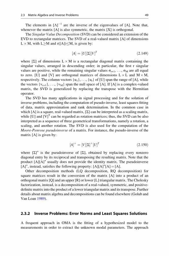
The Singular Value Decomposition (SVD) can be considered an extension of theEVD to rectangular matrices. The SVD of a real-valued matrix [A] of dimensions

LM, with L�M and r([A])�M, is given by:

A½ � ¼ U½ � Σ½ � V½ �T ð2:149Þwhere [Σ] of dimensions LM is a rectangular diagonal matrix containing the

singular values, arranged in descending order; in particular, the first r singular

values are positive, while the remaining singular values σr+1, . . ., σM are all equal

to zero. [U] and [V] are orthogonal matrices of dimensions LL and MM,

respectively. The column vectors {u1}, . . ., {ur} of [U] span the range of [A], whilethe vectors {vr+1}, . . ., {vM} span the null space of [A]. If [A] is a complex-valued

matrix, the SVD is generalized by replacing the transpose with the Hermitian

operator.

The SVD has many applications in signal processing and for the solution of

inverse problems, including the computation of pseudo-inverse, least squares fitting

of data, matrix approximation and rank determination. In the common case in

which [A] is a square, real-valued matrix, [Σ] can be interpreted as a scaling matrix,

while [U] and [V]T can be regarded as rotation matrices; thus, the SVD can be also

interpreted as a sequence of three geometrical transformations, namely a rotation, a

scaling, and another rotation. The SVD is also used for the computation of the

Moore-Penrose pseudoinverse of a matrix. For instance, the pseudo-inverse of the

matrix [A] is given by:

A½ �þ ¼ V½ � Σ½ �þ U½ �T ð2:150Þwhere [Σ]+ is the pseudoinverse of [Σ], obtained by replacing every nonzero

diagonal entry by its reciprocal and transposing the resulting matrix. Note that the

product [A][A]+ usually does not provide the identity matrix. The pseudoinverse

[A]+, instead, satisfies the following property: [A][A]+[A]¼ [A].

Other decomposition methods (LQ decomposition, RQ decomposition) for

square matrices result in the conversion of the matrix [A] into a product of an

orthogonal matrix [Q] and an upper [R] or lower [L] triangular matrix. The Cholesky

factorization, instead, is a decomposition of a real-valued, symmetric, and positive-

definite matrix into the product of a lower triangular matrix and its transpose. Further

details about matrix algebra and decompositions can be found elsewhere (Golub and

Van Loan 1989).

2.3.2 Inverse Problems: Error Norms and Least Squares Solutions

A frequent approach in OMA is the fitting of a hypothesized model to the

measurements in order to extract the unknown modal parameters. The approach


to fitting depends on the selected model. For the sake of clarity, in this section

the main concepts are illustrated with reference to a very simple and general

polynomial function:

y xð Þ ¼ c0 þ c1xþ c2x2 þ . . .þ cL�1x

L�1 ð2:151ÞNo specific references are made to the theoretical background of OMA at this

stage, but the application of these concepts in different contexts is straightforward

and it will become clearer when the theory of some OMA methods is reviewed

in Chap. 4.

Assuming that M measurements have been carried out, the L unknown model

parameters (c0, c1, . . ., cL-1) can be determined from the following set of M

equations:

y1 ¼ c0 þ c1x1 þ c2x21 þ . . .þ cL�1x

L�11

. . .yi ¼ c0 þ c1xi þ c2x

2i þ . . .þ cL�1x

L�1i

. . .yM ¼ c0 þ c1xM þ c2x

2M þ . . .þ cL�1x

L�1M

ð2:152Þ

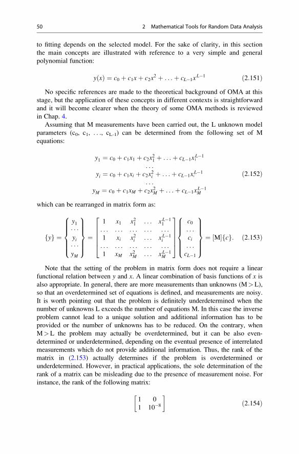
which can be rearranged in matrix form as:

yf g ¼

y1� � �yi� � �yM

8>>>><>>>>:

9>>>>=>>>>;

¼

1 x1 x21 . . . xL�11

. . . . . . . . . . . . . . .1 xi x2i . . . xL�1

i

. . . . . . . . . . . . . . .1 xM x2M . . . xL�1

M

266664

377775

c0. . .ci. . .cL�1

8>>>><>>>>:

9>>>>=>>>>;

¼ M½ � cf g: ð2:153Þ

Note that the setting of the problem in matrix form does not require a linear

functional relation between y and x. A linear combination of basis functions of x isalso appropriate. In general, there are more measurements than unknowns (M>L),

so that an overdetermined set of equations is defined, and measurements are noisy.

It is worth pointing out that the problem is definitely underdetermined when the

number of unknowns L exceeds the number of equations M. In this case the inverse

problem cannot lead to a unique solution and additional information has to be

provided or the number of unknowns has to be reduced. On the contrary, when

M>L the problem may actually be overdetermined, but it can be also even-

determined or underdetermined, depending on the eventual presence of interrelated

measurements which do not provide additional information. Thus, the rank of the

matrix in (2.153) actually determines if the problem is overdetermined or

underdetermined. However, in practical applications, the sole determination of the

rank of a matrix can be misleading due to the presence of measurement noise. For

instance, the rank of the following matrix:

1 0

1 10�8

�ð2:154Þ


http://dx.doi.org/10.1007/978-1-4939-0767-0_4

is 2 but the second row can be considered linearly dependent on the first row from

the practical point of view, since it does not provide a significant contribution of

information to the solution of the inverse problem. In similar conditions the SVD of

the matrix can provide more valuable information about the type of inverse

problem. In fact, the condition number κ, defined as the ratio between the maximum

and minimum absolute values of singular values, can be computed to assess if the

matrix is noninvertible (κ¼1), ill-conditioned (κ very large) or invertible (small

κ). Since the small singular values in ill-conditioned problems magnify the errors,

considering only the subset of the largest singular values can reduce their effect.

The selection of the number of singular values to be retained is usually based on

sorting of the singular values and identification of jumps; in the absence of jumps, a

selection ensuring numerical stability is carried out.

Assuming that a curve fitting the measured data has been found and the

functional relation between y and x in (2.151) has been established, there will be

an error (or residual) associated to the i-th measurement. It can be computed as

difference between the predicted (yi,pred) and the measured (yi,meas) value of y:

εi ¼ yi,meas � yi,pred ð2:155Þ

Thus, the objective of the analysis is the estimation of the unknown coefficients

(c0, c1, . . ., cL-1) from the measured data in a way able to minimize the sum of the

residuals when all measurements are taken into account.

Different definitions for the residuals can be adopted, taking into account that the

selected error definition has an influence on the estimation of the unknown

parameters. For instance, when the data are characterized by the presence of very

large and very small values in the same set, the computation of the residuals

according to (2.155) biases the inversion towards the largest values. As an alterna-

tive, one of the following definitions of residual can be considered:

εi ¼yi,meas � yi,pred

yi,predproportional errorð Þ ð2:156Þ

εi ¼ log yi,meas� �� log yi,pred

� �log differenceð Þ ð2:157Þ

Additional error definitions can be found in the literature (see, for instance,

Santamarina and Fratta 2005).

A global evaluation of the quality of the fit can be obtained from the computation

of the norm of the vector of residuals {ε}:

εf g ¼

ε1::::εi::::εM

8>>>><>>>>:

9>>>>=>>>>;

ð2:158Þ


The generic n-norm is given by:

Ln ¼ffiffiffiffiffiffiffiffiffiffiffiffiffiffiffiffiXi

εij jnn

r: ð2:159Þ

The order of the norm is related to the weight placed on the larger errors:

the higher the order of the norm, the higher the weight of the larger errors.

Three notable norms are:

L1 ¼Xi

εij j ð2:160Þ

L2 ¼ffiffiffiffiffiffiffiffiffiffiffiffiffiffiffiffiXi

εij j2r

¼ffiffiffiffiffiffiffiffiffiffiffiffiffiffiffiffiffiεf gT εf g

qð2:161Þ

L1 ¼ max ε1j j; . . . ; εij j; . . . ; εMj jð Þ: ð2:162ÞThe L1 norm provides a robust solution, since it is not sensitive to a few large

errors in the data; the L2 norm is compatible with additive Gaussian noise present in

the data; the L1 norm considers only the largest error and, as a consequence, is the

most sensitive to errors in the data.

Based on the previous definitions, the least squares solution of the inverse

problem can be defined as the set of values of the coefficients (c0, c1, . . ., cL-1)that minimizes the L2 norm of the vector of residuals. Thus, setting the derivative of

this L2 norm with respect to {c} equal to zero, under the assumption that [M]T[M] is

invertible the least squares solution provides the following estimate of the model

parameters:

cf g ¼ M½ �T M½ � ��1

M½ �T ymeasf g ¼ M½ �þ ymeasf g: ð2:163Þ

The least squares method is a standard approach to the approximate solution of

overdetermined systems. However, it works well when the uncertainties affect the

dependent variable. If substantial uncertainties affect also the independent variable,

the total least square approach has to be adopted. It is able to take into account the

observational errors on both dependent and independent variables. The mathematical

details of the method are out of the scope of the book, and the interested reader can

refer to (Golub and Van Loan 1989) for more details. However, it is worth recalling

the geometrical interpretation of the total least squares method in comparison with

the least squares approach. In fact, when the independent variable is error-free, the

residual represents the distance between the observed data point and the fitted

curve along the y direction. On the contrary, in total least squares, when both

variables are measured in the same units and the errors on both variables are the

same, the residual represents the shortest distance between the data point and the

fitted curve. Thus, the residual vector is orthogonal to the tangent of the curve.


2.4 Applications

2.4.1 Operations with Complex Numbers

Task. Create a calculator to carry out the following operations with complex

numbers:

• Get real part and imaginary part of a complex number;

• Get amplitude and phase of a complex number;

• Compute complex conjugate of a complex number;

• Compute sum, product, and division between two complex numbers;

• Compute amplitude and phase of 1 + 0i and 0 + 1i;

• Compute: (1 + 0i) + (0 + 1i), (1 + 0i) * (0 + 1i), (1 + 0i)/(0 + 1i); (1 + 1i) + (1-1i),

(1 + 1i) * (1-1i), (1 + 1i)/(1-1i).

Suggestions. This is a very simple example to get confidence with the LabVIEW

environment and with basic operations with complex numbers. In the design of the

user interface on the Front Panel, place controls and indicators and set in their

properties a complex representation of the data (right click on the control/indicator,

then select “Representation” and “Complex Double CDB”). Then, write the code

in the Block Diagram (CTRL+E to open it from the Front Panel). Algebraic

operators are in the Functions Palette under “Programming – Numeric”; the

operations on complex numbers are under “Programming – Numeric – Complex.”

Appropriately connect controls and indicators. Use the While Loop structure under

“Programming – Structures” to develop a simple, interactive user interface. It is

possible to define the timing in the execution of the cycles by means of the “Wait

Until Next ms Multiple.vi” in “Programming – Timing.”

Sample code. Refer to “Complex values – calculator.vi” in the folder “Chapter 2” of

the disk accompanying the book.

2.4.2 Fourier Transform

Task. Compute the DFT of the following signals:

• Sine wave at frequency f¼ 3 Hz,

• Sine wave at frequency f¼ 6 Hz,

• Constant signal,

• Combinations of the previous signals,

and analyze how the magnitude and phase spectra change when:

• The windowed signal is periodic (for instance, when N is a multiple of 100),

• The windowed signal is not periodic (truncated),

• The length of the signal is doubled.

Consider a sampling interval Δt equal to 0.01 s, which implies a sampling

frequency fs¼ 100 Hz fmax¼ 6 Hz.

Suggestions. In the design of the user interface on the Front Panel, place a control

to input the number of data points N; place three “WaveformGraph” controls (it is in

2.4 Applications 53

the Controls Palette under “Modern – Graph”) to show the signal in time domain and

the amplitude and phase spectra in frequency domain. In the BlockDiagram place the

“Sine.vi” (it can be found in the Functions Palette under “Mathematics – Elementary

– Trigonometric”); use a “For Loop” structure (it can be found in the Functions

Palette under “Programming – Structures”) to generate signals of the desired length.

Transform the obtained arrays of Double into Waveform type of data by wiring the

sampling interval and the array of values of the signal to the “Build Waveform.vi”

(it can be found in the Functions Palette under “Programming – Waveform”).

Compute the Fourier Transform of the signals by means of “SVT FFT Spectrum

(Mag-Phase).vi” (“Addons – Sound & Vibration – Frequency Analysis – Baseband

FFT”). Appropriately connect controls and indicators. Use the While Loop structure

under “Programming – Structures” to develop a simple, interactive user interface. It is

possible to define the timing in the execution of the cycles by means of the “Wait

Until Next ms Multiple.vi” in “Programming – Timing.”

Sample code. Refer to “FFT mag-phase.vi” in the folder “Chapter 2” of the disk

accompanying the book.

2.4.3 Statistics

Task. Compute mode, mean, maximum and minimum value, standard deviation,

and variance of the data in “Data for statistics and histogram.txt” in the folder

“Chapter 2\Statistics” of the disk accompanying the book. Use the data to plot a

histogram. Pay attention to the obtained results for different values of the number of

intervals.

Suggestions. Use the “Read from Spreadsheet File.vi” to load the data from file.

Maximum and minimum value in the data can be identified by means of the “Array

Max & Min.vi” under “Programming – Array.” Mean, standard deviation, and

variance can be computed by means of the “Std Deviation and Variance.vi” under

“Mathematics – Probability and Statistics.” In the same palette there are “Mode.vi”

and “Histogram.vi,” which can be used to compute the mode and plot the histogram.

Place a “XY Graph” on the Front Panel to plot the resulting histogram.

Sample code. Refer to “Statistics and histogram.vi” in the folder “Chapter 2\Statistics”

of the disk accompanying the book.

2.4.4 Probability Density Functions

Task. Plot the standardized probability density function of a sine wave in noise

(2.62) for different values of the variance ratio defined in (2.63).

Suggestions. Use the “For Loop” to set the vector of values of the standardized

variable z where the probability density function will be computed. Compute

the variance of the Gaussian noise from the values of the variance ratio. Use a


“For Loop” to compute the values of the function in the integral at the selected values

of z. Use the “Numeric Integration.vi” under “Mathematics – Integration & Differ-

entiation” to compute the integral. Put the arrays of the values of z and p(z) into a

cluster (use the “Bundle.vi” under “Programming – Cluster & Variant”), create an

array of the plots of p(z) and show them in a “XY graph” on the Front Panel.

Sample code. Refer to “Sine wave in Gaussian noise.vi” in the folder “Chapter 2” ofthe disk accompanying the book.

2.4.5 Auto- and Cross-Correlation Functions

Task. Compute and plot all the possible auto- and cross-correlation functions from

the data in “Sample record 12 channels – sampling frequency 10 Hz.txt” in the

folder “Chapter 2\Correlation” of the disk accompanying the book. Data in the file

are organized in columns: the first column gives the time; the next 12 columns

report the data for each of the 12 time histories.

Suggestions. Use the “Read from Spreadsheet File.vi” to load the data from file.

Compute the auto-correlation functions associated to the 12 time series and the

cross-correlation between couples of records. Use the formula (2.96) for the direct

estimation of correlation functions, eventually organizing the data into matrices

and taking advantage of the matrix product. Organize the resulting data into a 3D

matrix so that one of its dimensions is associated to the time lag, and at a certain

time lag a square matrix of dimensions 12 12 is obtained. Use the “While Loop”

to create a user-interface for the selection of one of the auto- or cross-correlation

functions from the matrix. Plot the data into a “Waveform Graph” placed on the

Front Panel.

Sample code. Refer to “Correlation function.vi” in the folder “Chapter 2\Correlation”of the disk accompanying the book.

2.4.6 Auto-Correlation of Gaussian Noise

Task. Generate a Gaussian white noise, compute its mean, variance, and standard

deviation, and plot its autocorrelation function. Use the “AutoCorrelation.vi” under

“Signal Processing – Signal Operation.”

Suggestions. Use the “Gaussian white noise.vi” under “Signal Processing – Signal

Generation” to generate the data. Use the “While Loop” structure to create a user-

interface for the selection of the parameters (number of samples and standard

deviation of simulated data) for data generation. Place the appropriate controls

for such parameters on the Front Panel. Use the “AutoCorrelation.vi” under “Signal

2.4 Applications 55

Processing – Signal Operation” to compute the auto-correlation function. Plot the

data into a “Waveform Graph” placed on the Front Panel.

Sample code. Refer to “Statistics and auto-correlation of Gaussian noise.vi” in the

folder “Chapter 2” of the disk accompanying the book.

2.4.7 Auto-Power Spectral Density Function

Task. Compute (according to the Welch procedure) and plot the auto-spectral density

functions of the data in “Sample record 12 channels – sampling frequency 10 Hz.txt”

(see Sect. 2.4.5). Divide the time series into a user-selectable number of segments;

consider a 50 % overlap of the data segments. Analyze the effects of windowing and

number of segments on the resulting spectra and the frequency resolution.

Suggestions. Create a SubVI that, given a time history, the number of segments and the

sampling frequency, provides an array of waveform data, where each waveform

consists of a (partially overlapping) data segment, and the number of data segments

nd. Take advantage of the “For Loop” structure to divide the total record into ndsegments. In the main VI, use the “Read from Spreadsheet File.vi” to load the data

from file. Compute the sampling frequency from the sampling interval. Select one

time history in the dataset and send it to the previously mentioned SubVI to divide it

into partially overlapping segments. Use the “For Loop” structure and the “SVT

Power Spectral Density.vi” under “Addons – Sound & Vibration – Frequency Analy-

sis – Baseband FFT” to compute the averaged PSDs. Plot the results into a “Waveform

Graph” placed on the Front Panel. Use the “While Loop” structure to create a user-

interface for the selection of the time histories and the analysis parameters.

Sample code. Refer to “Averaged PSD.vi” and “Overlap 0.5.vi” in the folder

“Chapter 2\PSD and overlap” of the disk accompanying the book.

2.4.8 Singular Value Decomposition

Task. Create a matrix [A] of dimensions 8 8 and whose entries are random

numbers. Create a constant matrix [B] of dimensions 8 8 and rank r([B])¼ 6.

Compute the matrices [A] + [B] and [A][B]. For each of the previously men-

tioned matrices compute the SVD, plot the obtained singular values after they

have been normalized with respect to the largest one, compute the condition

number.

Suggestions. Use the “Random number (0-1).vi” under “Programming – Numeric”

and two “For Loop” structures inside each other to create [A]. The matrix multipli-

cation can be carried out by the “AB.vi” under “Mathematics – Linear Algebra.”


The SVD can be carried out by the “SVD Decomposition.vi” under “Mathematics –

Linear Algebra.”

Sample code. Refer to “SVD and rank of a matrix.vi” in the folder “Chapter 2” of

the disk accompanying the book.

References

Bendat JS, Piersol AG (2000) Random data: analysis and measurement procedures, 3rd edn.

Wiley, New York, NY

Cantieni R (2004) Experimental methods used in system identification of civil engineering

structures. In: Proc 2nd Workshop Problemi di vibrazioni nelle strutture civili e nelle

costruzioni meccaniche, Perugia

Cooley JW, Tukey JW (1965) An algorithm for the machine calculation of complex Fourier series.

Math Comp 19:297–301

Golub GH, Van Loan CF (1989) Matrix computations. John Hopkins University Press,

Baltimore, MD

Heylen W, Lammens S, Sas P (1998) Modal analysis theory and testing. Katholieke Universiteit

Leuven, Leuven

Papoulis A (1991) Probability, random variables, and stochastic processes, 3rd edn. McGraw-Hill,

New York, NY

Santamarina JC, Fratta D (2005) Discrete signals and inverse problems: an introduction for

engineers and scientists. Wiley, Chichester

References 57

operational modal analysis of civil engineering structures || mathematical tools for random data...

Documents