DOCIIJJT 2231112

29 15f 472 Si 024 424

AUTHOR West, Alfred N.TITLE Operational Control Procedures for the Activated

Sludge Process: Appendix.INSTITUTION Environmental Protection coucy, Vashingtcm, D.C.

Office cf Mater Programs.REPORT NO EPA-330/9-74-001dPUB DATE Bar 74NOTE 37p.; For related documents, see SE 024 421-423:

Graphs and charts may not reproduce well

EDI; PRICE EF-30.83 HC -$2.06 Plus Postage.DESCRIPTORS *Environmental Technlcians; *Instructional Baterials;

*Job Skills; Laboratory Training; Banageaent;*Beasurement Techniques; Polluticn; *Post SeccndaryEducation; Waste Dispcsal; *Water PollutionControl

IDENTIFIERS Activated Sludge; *Neste Water Treatment; laterQuality

ABSTRACTThis document is the appendix fcr a series cf

documents developed by the National Training and OperationalTechnology Center describing operational control procedures for theactivated sludge process used in astevater treatment. Categoriesdiscussed include: control test data, trend charts, acving averages,semi-logarithmic plots, probability plot examples, testing Equipmentand symbols and terminology. (CS)

****************Reproducti

*

****************

*******************************************************ons supplied by EDRS are the best that can be made

from the original document.*******************************************************

S DEPARTMENT OF NNOUCATtON WELFARE

NATIONAL INSTITUTE OFEDUCATION

.,, Dot uoRE rS SEEM REPRO-DUCE D FAA( Ti r S RECE.VED E a am

Pt ff SON OR oRG04. DO' ION ORIGIr.-T MC, IT POOR TS OE VIE 04 OR OPINIONSSTATED 00 ROT PECESSMOL v REPRE-SENT Os i.C 1111'.01111L INSTITUTE OEE DuC T ION POSITION OR PER, .r V

NATIONAL WASTE TJEATMENT CENTER

ONONNATI

OPERATIONAL CONTROL PROCEDURES

for the

ACTIVATED SLUDGE PROCESS

APPENDIX

MARCH 1974

UNITED STATE* ENVIRONMENTAL PROTECTION AGENCYOFFICE OF WATER PROGRAM OPERATIONS

.1011° Etr4%

ai; ti

tAlra

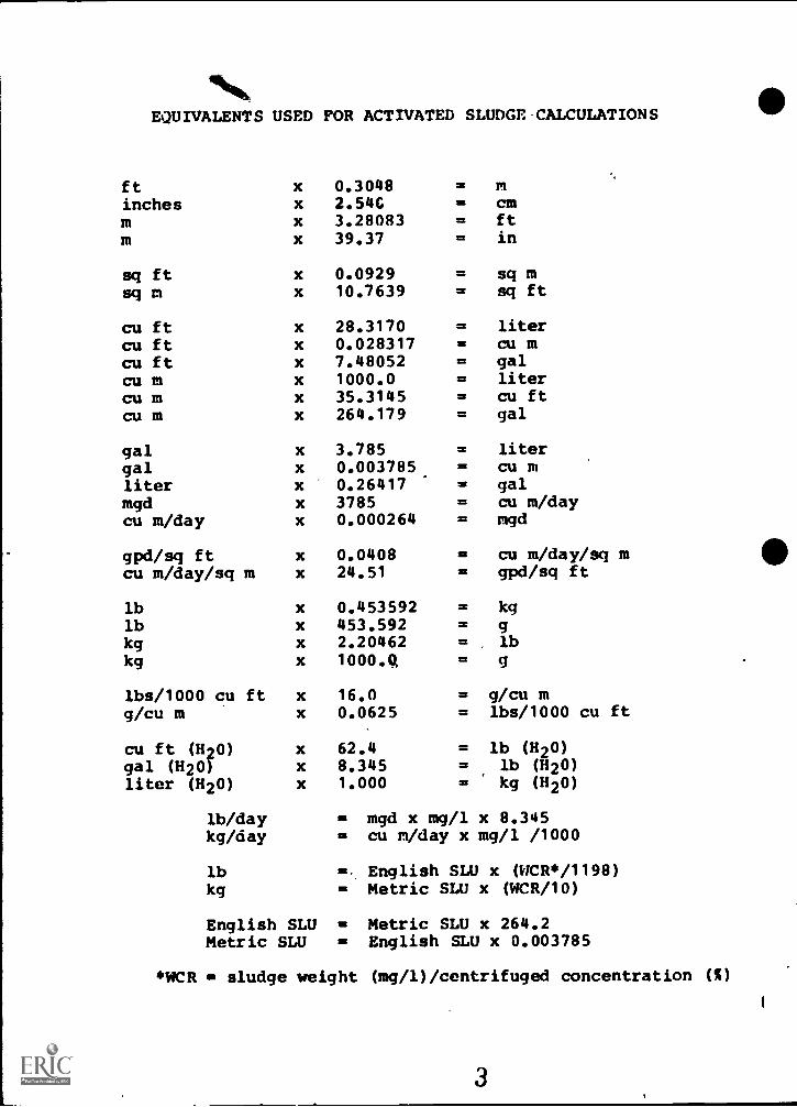
EQUIVALENTS USED FOR ACTIVATED SLUDGE-CALCULATIONS

ftinchesmm

sq ft

xxxx

x

0.30482.5463.2808339.37

0.0929

====

cmftin

sq mSCI Li x 10.7639 sq ft

cu ft x 28.3170 litercu ft x 0.028317 cu mcu ft x 7.48052 galcu m x 1000.0 litercu m x 35.3145 cu ftcu m x 264.179 gal

gal x 3.785 litergal x 0.003785 cu mliter x 0.26417 galmgd x 3785 cu m/daycu m/day x 0.000264 mgd

gpd/sq ft x 0.0408 cu m/day/sq mcu m/day/sq m x 24.51 = gpd/sq ft

lb x 0.453592 = kglb x 453.592 = gkg x 2.20462 = lbkg x 1000.4X = g

lbs/1000 cu ft x 16.0 = g/cu mg/cu m x 0.0625 = lbs/1000 cu ft

cu ft (H20) x 62.4 = lb (H20)gal (H20) x 8.345 = lb (H20)liter (H20) x 1.000 = kg (H20)

lb/daykg/day

lbkg

English SLUMetric SLU

mgd x mg/1cu re/day x

x 8.345mg/1 /1000

= English SLU x (WCR*/1198)= Metric SLU x (WCR/10)

WCR = sludge weight

Metric SLU x 264.2English SLU x 0.003785

00;M/centrifuged concentration (%)

3

NATIONAL WASTE TREATMENT CENTER - CINCINNATI

OPTTIONAL CONTROL PROCEDURES

/ FOP THE

ACTIVATED SLUDGE PROCESS

APPENDIX

by

Alfred W. West, P.E.

Director, National Waste Treatment Center(formerly Waste Treatment Branch, National Field

Investigations Center - Cincinnati)

MARCH 1974(Revised Nov.,1975)

UNITED STATES ENVIRONMENTAL PROTECTION AGENCY

OFFICE OF WATER PROGRAM OPERATIONS

4

FOREWORD

The National Waste Treatment Center (Cincinnati) is

developing a series of pamphlets describing OperationalControl Procedures for the Activated Sludge Process. This

series, describing the 'NWTC Procedures", will include PartI OBSERVATIONS, Part II CONTROL TESTS, Part III CALCULATIONPROCEDURES, Part IV SLUDGE QUALITY, Part V PROCESS CONTROLand an APPENDIX. 4ach of these individual parts will bereleased for distribution as soon as it is completed, though

not necessarily in numerical order. the original five-partseries may then be expanded to include case histories andrefined process evaluation and control techniques.

This pamphlet has been developed' as a reference forActivated Sludge Plant Control lectures I have presented attraining sessions, symposia, and workshops. It is based onmy personal conclusions reached while directing the

operation of dozens of different activated sludge plants.This pamphlet is not necessarily an expression ofEnvironmental Protection Agency policy or requirements.

The mention of trade "names or commercial products inthis pamphlet is for illustrative purposes and does Lot

constitute endorsement or recommendation for use by theEnvironmental Protection Agency.

Alfred N. West

TALE OF CONTENTS

PAGE NO.

Control Test Data 1

Trend Charts

Moving Averages 7

Semi-Logarithmic Plots 11

Probability Plot Examples 14

Testing Equipment 20

Symbols and Terminology 23

6

TwIE

CONTROL TEST DATA

WASTEWATER TREATMENT PLANT

DAY

DATE

A C

24 HR AVG(TOTALIZER;

FLOWSIASODI

AF1 24NSF 4XSF

AF1NSFXSF

AFIRSFXSF

AF1

RSFXSF

SST SSV SSC SSV SSC1000

SSC1000

SWO 4....e.' 1000 . -. - -.S ezo .5.4.. .70,,, 4 ,, 4,, + c-

. .... -;-,

,I, 39 9...7.= - 2 . S -=S -5 -5...., -.4. r-- .-,̂

9 SS 600 .4 z"-; 1;C" 7.2 "" S t

it 10 _ 720 ...: 15 1, .i.2c: 202 2S SZc0 30 45c

40 400 ;1- SO 545c .to SO

. SG 4fc 8 PGS 4 5C 9'C'3'

RISETIME , MRS MRS FIRS

4

Z - ATCf. 2 it Inc4.; xscSLUDIIE

SUIMKET DOSDEPTI4

TURBID-MAETER 14"""

ATCRSCXSC

ATCRSCXSC

(NATIONTANK00

C

.1111. WIT1-HR

DOB

INIT1 HR

INIT1-HR

INOUT

RAWA T.

MIDNIGHT TOTALIZER READING

RAWAT

MI 't :ca NSF 423gta_S XSF

COMMENTS and SPECIAL DATA1000 - 40o Nn - ekim cANWeD F-` =L, P." cm

7

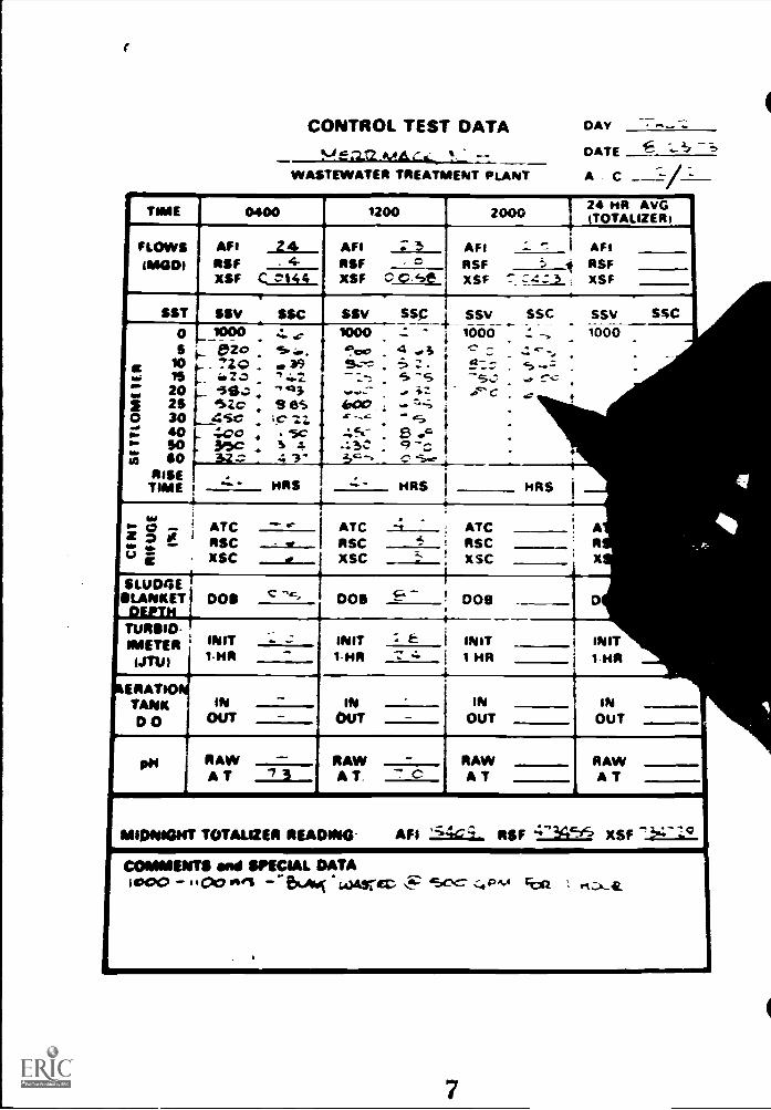
CONTROL TEST DATA

Data from the control tests described in Part IIControl Tests should be recorded in an organized manner ateach test period. A generalized data sheet suitable forthis purpose is shown on the facing page.

The test times shown near the top of the sheet will notbe standard for each plant but will normally be determinedby personnel shift changes and diurnal floe or loadvariation. At times additional centrifuge and depth ofblanket tests may be desireable. These data may be recordedat the bottom of the sheet under comments and special data.

Except for the Settled Sludge Concentration (SSC)values, all numbers recorded on the data sheet are observedvalues. The SSC's are calculated as described in Part IIIA

Calculation Procedures.

The- two sketches below illustrate how the 0400centrifuge and settloneter test data were used to developSettled Sludge Volume (SSV) and Settled Sludge Concentration(SSC) curves to help analyze sludge quality.

A seperate column is provided on the data sheet foraveraging the days' data. Plows recorded in this columnshould be totalizer values. These daily average values willbe further used to calculate moving averages and additionalprocess parameters.

le W. If 7 IS14,,4 00 OtGO rM 1111,

1

8

1141T-Vit YINI 1.1111 int

1

H

DOB

--k

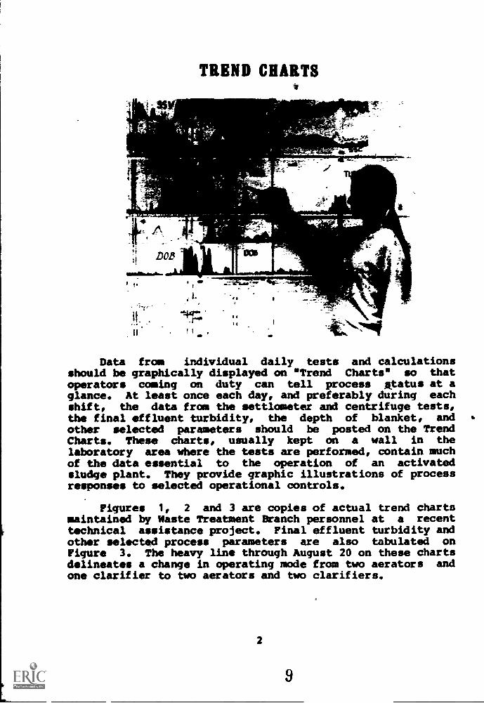
TREND CHARTS

t. 'I

Data from individual daily tests and calculationsshould be graphically displayed on "Trend Charts" so thatoperators coming on duty can tell process status at aglance. At least once each day, and preferably during eachshift, the data from the settlometer and centrifuge tests,the final effluent turbidity, the depth of blanket, andother selected parameters should be posted on the TrendCharts. These charts, usually kept on a wall in thelaboratory area where the tests are performed, contain muchof the data essential to the operation of an activatedsludge plant. They provide graphic illustrations of processresponses to selected operational controls.

Figures 1, 2 and 3 are copies of actual trend chartsmaintained by Waste Treatment Branch personnel at a recenttechnical assistance project. Final effluent turbidity andother selected process parameters are also tabulated onFigure 3. The heavy line through August 20 on these chartsdelineates a change in operating mode from two aerators andone clarifier to two aerators and two clarifiers.

2

The symbols, control tests and calculation proceduresfor determining the parameters illustrated on Figures 1, 2and 3 have been explained in previous Parts of this series.For convenient referencing, all _symbols used in thispamphlet series and their definitions are restated inalphabetical order on pages 23 through 27.

It should be kept in mind that trend charts such asthese are really work sheets and are appropriate places forposting notes or data that might otherwise be recolided in alog book and then forgotten. For example, unusualoccurrences that might affect plant performance, such asslugs of strong industrial wastes or toxic chemicalsentering the plant, heavy rains, power failures, etc. can benoted directly on the trend charts. If this is done,reasons for sudden upsets or process imbalance can be easilyidentified.

When time permits, trend charts may be expanded toprovide plant personnel with greater insights into theoperation of their treatment plant. Certain informationshould be drawn on semi-log paper to help determinerelationships between various process parameters, and themoving averages developed to damp out any large day-to-dayvariations that occur.

3

r

.1160a

._ 40,yea

44 f its t 04 A:K

4

100

G -11,1 -1- W

I.: it, 17

7 F14.

HA VOUJr /P7.5

w T F.

, i 2L' - 2 ..,

Figure 1

TYPICAL TREND CHART SHOWING SSV 6 SSC CURVES

11

80

vT

0*X

/ft2

4

1_t°

W.* =1'_41,4yst

A;si

13 11- IS I

Figure 2

r T r s

TYPICAL TREND CHART SHOWING XSUiday & DOB CURVES

1

AF I 246 2.65 2.34rasy 54 .264 .2443

XSF .029 .034 33

AMOR. 163 149 141

4509110000 19.t Sit 191

F/M 35 14 15

MEgusimizic 11 H WTF

FLOWS (riejd)265 238 1.195 I_595 2 26 215 2 638 2 MI 2 204 1 575 1 455 2 60C.265 .403 A96 .519 .545 S24 1034 1310 126 I049 .750 .961

.033 .063 .050 .026 .051 056 .041 .055 .044 .012 .30 .081

.0., 124.71014 TANK CHARACTERISTICS

149 * 190 20.6 $33 122 II 6 Ilb 11.6 .165 iv 7 12223.7 53S 240 11.0 20.2 436 334 454 228 194 30.1 sae

.17 24 .16 07 .13 .V. .22 is 105 .005 .14%. .189

ci 0962 144, Sty 44/39 11!'3253/24 8oh4 1'64.2 34.2. 34i2; 144 3+3.0 3.%7 3S4 o

F144.1. CLARIFIER CHARACTEQISTICS

600 330 401. 34.1 341 311 248 299 240 rib Ma 254107 .79 .76 A7 1.20 96 1.01 173 1.22 103 .97 1 57

11.5 19.2 504 341 244 321 41.1 443 49.2 72.1 SOA 404

OFI2 361 WO 330CSDT .97 .09 .99

CFP 4 11.3 ILO

COO

SS

rt

GS30

II

36II.

10

549

0

num. ecrwerr cauALrrYT I% S 4. 4 12 S 5.0 .2 2 2 3AS 66 40 55 S9 38 Ad. AZ 59 59 34 '5112 19 ID 7 6 4 6 11 1 5 3 20

AUG-057%.73

Figure 3

A

TYPICAL TREND CHART SHOWING FINAL EFFLUENT TURBIDITY

AND A TABULATION OF SELECTED PROCESS PARAMETERS

13

MOVING AVERAGES

Moving averages, especially ,those for 7- and 28-dayintervals, are useful fot evaluating process responses tooperational control adjustments. The effects of a majorchange in operating procedures are usually confirmed about aweek after the start of the new control procedures., Thedevelopment of a stable sludge, fully acclimated to thechange, usually takes about a month.

The 7-day moving average (7DMA), which reflects theeffects of low load Saturdays and Sundays as well as highload Mondays and Tuesdays, permits a realistic review ofmedium term process response. The 28-day moving average(28DMA) permits evaluation of long-term stabilizationperformance.

Figure 4 is a graph of sludge wasting dadaily, data points, the 7-day_moving average,moving average. The individual dataconsiderable variation from day to day. By plmoving average, the large variations are smthe actual trends (increasing or decreasingbecame more apparent. The 28-day moving average shows the

showing thethe 28-day

into showing a 7-daythed out and

sting rates)

long term trends.

Table 1 includes the daily'(24 hour) average, and the7-day and 28-day moving average data that are plotted onFigure 4.

The 7-day moving average for any given day is theaverage of the data for that day and the six previous days.For example, from Table 1, the 7-day moving average for1/4/73 is 1.932. This is obtained by averaging the data for1/4/73 and the six previous days, starting with 12/29/72:

12/29/7212/30/7212/31/72

5.0580.01,374

1/ 1/73' 2.4591/ 2/73' 0.9601/ 3/73 1.5981/ 4/73 2.076

7 /13.525

1.932 7-day moving a44.

14

1009.080

,as TO

8 60

5.0

30

20

100.90.80.7

$ 0.6toU 0.5

11J

0.4

0.3

15

%,....

....

HOUR AVERAGE

-

.....11 a .. am%, ao.

..1. ems .... .....

TY??

...

28 DAYMOVING AVERAGE

7 DAY MOVING AVERAGE_

T .i, ZERO WASTING

13 20NOVEMBEIZ 1972

27

Figure 4

II 18DECL 1113ES2 1972

MOVING AVERAGE PLOTS OF XSU DATA

25 i

JAN 73

Table 1

24 HOUR AVERAGES, 7 DAY & 28 DAY MOVING AVERAGES OF XSU DATA

DATE kSU2914RA

XSU794A,

XSU284MA

DATE XSU24NPA

XSU70MA

XSU280MA

12/ 7/72 3.089 5.593 3.67711/ 6/72 BOUNDARY DATE 12/ 8/72 11.098 9.876 3.59311/ 6/72 6.678 6.678. 1 6.678. 1 12/ 9/72 9.831 5.105 3.37311/ 7/72 10.873 8.775- 2 8.775. 2 12/10/72 5.20 5.908 3.30611/ 8/72 9.259 8.937- 3 8.937. 3 17/11/72 5.791 5.753 3.30611/ 9/72 10.586 9.3119 9 9.399 12/12/72 6.750 5.275 3.5011/10/72 7.053 9.050. 5 9.050- 5 12/13/72 5.580 5.00 3.79611/11/72 9.600 9.1117- 6 9.192 12/19/72 5.058 5.329 3.92711/12/72 7.119 8.853 1.853. 7 12/15/72 5.364 5.509 4.11811/13/72 5.750 8.720 8.965. 8 12/16/72 3.1168 5.315 9.21011/14/72 0.0 7.167 7.5211. 9 12/17/72 9.568 5.190 9.33511/15/72 0.0 5.894 6.77210 12/18/72 6.1014 5.290 4.59211/16/72 0.0 9.332 6.15611' 12/19/72 9.399 4.959 4.65111/17/72 0.0 3.710 5.69312 1:/20/72 9.327 4.775 11.72911/18/72 0.900 1.967 5.278-13 12/21/72 3.037 4.987 4.79711/19/72 0.070 1.079 11.963.111 12/22/72 1.732 3.968 4.71111/20/72 0.630 0.393 9.67515 12/23/72 0.907 3.602 4.69511/21/72 1.350 0.536 11.116716 12/29/72 1.812 3.232 11.71011/22/72 2.160 0.8101 9.531.17 12/25/72 0.801 2.932 9.73811/23/72 2.520 1.209 9.23018 12/26/72 6.859 2.783 9.78611/24/72 2.736 1.595 9.152.19 12/27/72 19.019 4.167 5.05111/2S/72 ?.772 1.863 9.083.20 12/28/72 8.188 4.903 5.07811/26/72 0.0 1.738 3.88821 12/29/72 5.058 5.378 4.93311/27/72 0.0 1.698 3.712 -22 12/30/72 0.0 5.298 9.81711/21/72 5.508 2.792 3.790-23 12/31/72 1.379 5.185 9.75511/29/72 6.629 2.180 3.908.29 1/ 1/73 2.959 5.1122 4.72911/;0/72 7.421 3.580 9.048-25 1/ 2/73 0.960 4.580 4.39812/ 1/72 9.120 9.492 9.24326 1/ 3/73 1.598 2.805 9.19912/ 2/72 3.230 9.558 9.20627 1/ k/73 2.076 1.932 4.16312/ 3/72 3.120 5.003 9.167 1/ 5/73 1.577 1.935 4.07312/ 4/72 3.326 5.09 11.0117

12/ S/72 10.091 6.133 9.02012/ 6/72 7.182 6.713 3.995

LEGEND:

MU EXCESS SLUDGE UNITS WASTED (IN 1,000 SLOWL UNITS)24HRA 216-1101IR (DAILY) AVERAGI70MA 7-DAY MOVING AVERAGE2tOPA 28-DAY MOVING AVERAGE

BOUNDARY DATE THE FIRST DAY OF DATA mom IN THE CALCULATIONS

INDICATES THE NUMBER OF DAILY DATA POINTS INCLUDED IN THECALCULATIONS, WHERE LESS THAN 7 (OR 28) ARE AVAILABLE.

17

Similarly, the 7-day moving average for the next day,1/5/73, is the average of the data for that day and the sixprevious days, starting with 12/30/72:

12/30/7212/31/72

0.01.374

1/ 1/73 2.4591/ 2/73 0.9601/ 3/73 1.9981/ 4/73 2.0761/ 5/73 1.577

7 /10.044

1.435 = 7-day moving avg.

The 7-day moving average for 1/5/73 could also becalculated easily from the previous day's calculations bysubtracting the data for 12/29/72 (5.058) from the previous,day's subtotal (13.525), adding the data for 1/5/73 (1.577)and dividing by 7:

13.525- 5.058 (12/29/72)

8.467+ 1.577 (1/5/73)

7 /10.044

1.435 = 7-day moving avg.

A 28-day moving average is derived by the same type ofcalculation.

When working with a new set of data, such as at thestart of a new operational control phase, it is necessary tostart with a progressive average (rather than a 7-day movingaverage) until seven days of data are included. Note thatthe 7 DMA column on Table 1 does not start with a true 7-daymoving average, since the time period covered is less thanseven days. The initial values for the first 6 days shownin the 7 DNA column are progressive averages until 11/12/72,at which point they become true 7-day moving averages.Similarly, the initial values for the first 27 days in the28 DMA column are progressive averages until 12/3/72, whenthey become 28-day moving averages.

10

18

SEMI-LOGARITHMIC PLOTS

Process responses (SSV, ATC, SSC, turbidity, etc.) tocontrol adjustments are normally plotted on a test-by-testbasis to permit process evaluation. Semi-logarithmic plotsare useful hen one wishes to compare the rate of change ofvarious parameters to a process adjustment because itpermits direct observation of rate changes between theparameters regardless of their magnitudes.

Consider the following hypothetical example asdisplayed on the two graphs below. Two identical data sets(A and B) are plotted on each graph. The left graph isdrawn on rectangular coordinate paper, the right on semi-logarithmic paper. Note how readily the trend similaritybecomes apparent from a comparison of the semi-logarithmiccurves. In this example, the plotted parameters haveidentical slopes and remain parallel to each other. Therectangular plot of the same parameters does not readilydisplay that the rate changes, defined by their slopes, areidentical. The probable relationship between parameters Aand B might have been overlooked if only rectangularcoordinate paper had been used.

100

0S0

70

0s0

0

30

20

10

.44

RECTANGULAR PLOT

T

11

10090S0

70

19

0S0

030

20

100S

rA

SEMI LOGARITHMIC PLOT

F-7

Now consider two plots drawn fron the actual plant datashown below:

TABLE 2

Day/Date Turb(JTU)

CSDT(hrs)

M 12/18/72 9.93 0.69T 19 9.53 1.09W 20 9.13 1.73T 21 13.00 3.32F 22 12.33 3.17S 23 13.53 2.85S 24 13.87 3.96

M 12/25/72 21.67 4.04T 26 17.33 4.61W 27 19.00 3.36T 28 -/\-- 23.00 3.29F 29 17.67 2.81S 30 13.30 2.88S 31 9.80 2.29

M 1/1/73 6.90 1.36T 2 6,30 1,10W 3 6.10 0.84T 4 5.77 0.78F 5 8.10 0.92S 6 9.25 0.92S 7 6.57 0.91

M 1/8/73 6.47 0.69T 9 5.03 0.74W 1C 3.67 0.79T 11 5.40 1.43F 12 5.90 1.25S 13 10.90 1.49S 14 10,47 1.39

The upper illustration on Figure 5 shows a rectangularplot of final effluent turbidity and CSDT (Clarifier SludgeDetention Time) versus Time. The lower illustration is aplot of the same data on semi-logarithmic paper. Whenplotted on smatrlog paper, the similarity between the twocurves becopel evident. The possible cause and effectrelationship between CSDT and turbidity might have beenoverlooked if only rectangular paper had been used.

12

10 lllllllllllll i I 1 1

=

LX

0

1=2 i ..wt0

Al

et

ItsT T14 20V

SEMI - LOCI PLOT

I

I J A I, A 1 iiiiiiiiiiWAsisrm T T Or Sim Y W T F SSIHT WT S!Ve 25 WI 25 26 27 28 29 10 11 1 2 3 5 17 9 10 11 a 15 WI

I

Figure 5

COMPARISON OF RECTANGULAR AND SEMILOGARITHMIC PLOTS

21

too10007060SO

ao

30 /

20 .

ato 12

LL

LL/

3QJ

Z

PROBABILITY PLOT EXAMPLES

When collected data are plotted on probability paper,they can be used to predict frequencies at which certainevents may occur. For example, from a probability plot ofpast treatment plant data, one may estimate the percentageof time that the hydraulic capacity of the plant may beexceeded, and the percentage of time that the final effluentquality may be less than acceptable limits.

Two examples of probability plots are presented.Bacteriological data, conforming to logarithmic growthrates, are usually plotted on probability paper with alogarithmic vertical scale (Figure 6). Chemical data areusually plotted on probability paper with a uniformlydivided vertical scale (Figure 7).

The first step in preparing a probability plot consistsof reorganizing the raw data, regardless of collecjion date,into an orderly progression starting with the smallestnumber and finishing with the largest. Such a progressionof 50,000 through 1,600,000+ for the 13 bits of data in thefirst example is shown in the second colymn of Table 3.

TABLE 3

COLIFORM PROBABILITY PLOT EXAMPLE

Coliform Density - MP /100 mlRanked in

Tabulated AscendingChronologically Order

"Exact"PlottingPositionN 13

110,000 50,00050,000 78,000 12.2

820,000 110,000 19.2220,000 130,000 27.3

1,600,000 220,000 34.9350,000 230,000 42.5110,000 330,000 50.0700,000 350,000 57.5130,000 700,000 65.1820,000 820,000 72.7

1,600,000 + 820,000 80.2230,000 1,600,000 87.878,000 1,600,000 + 95.2

NOTE: 541,000330,000

Arithmetic MeanProbability Mean (Fig. 7)

14

22

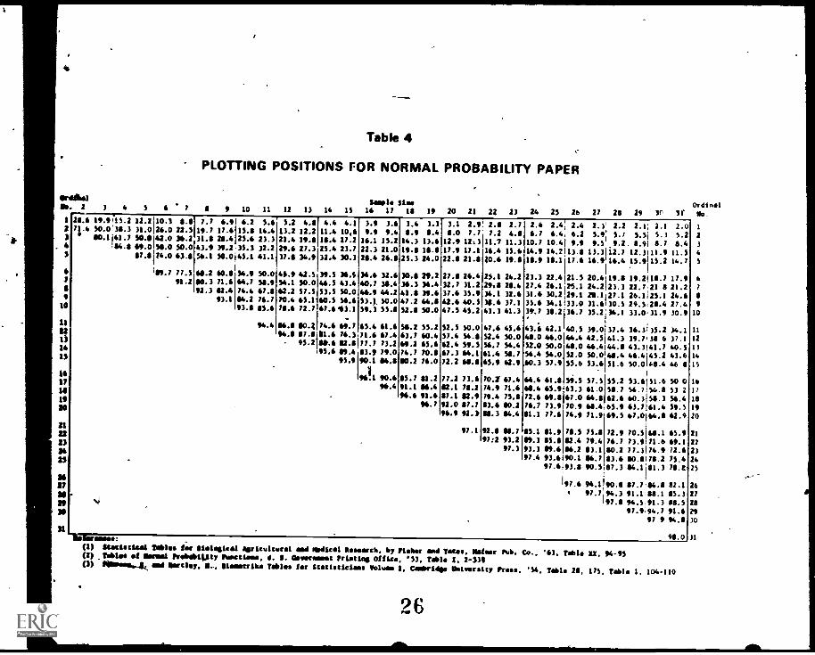
The plotting position, shown in the third column ofTable 3 for each data item, can then be obtained directlyfrom Table 4 if 50 or less data points are to be plotted.Plotting positions for sample sizes greater than 50 can becalculated according to the formula on Table 4, page 18.For this sample size of 13, the plotting positions rangedfrom 'less than 4.8% of the time for 50,000 to 'less than"95.2% of the time for 160,000+.

The coliform concentrations were then plotted accordingto their respective plotting positions. The completedprobability 'plot of the conform data is illustrated inFigure 6.

At first glance, the large and irregular day-to-daydifferences- in coliform concentrations shown in column oneof Table 3 appeared *irreconcilable. But the probabilityplot of this same infnrmation displayed the data in anorderly fashion and permitted logical evaluation of thesurvey results. As shown on Figure 6, the mean density was330,000 MPN /100 ml and it could be expected that theconcentration would most probably equal or exceed 58,000 90%of the time& and equal or exceed 1,850,000 10% of the time.

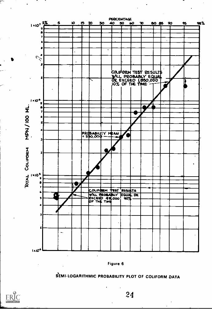
Figure 7 is a probability plot of final effluent BOBSconcentrations and aeration tank DODS loadings at anactivated sludge plant. The data were arranged as in theprevious example, and the plotting positions were determinedfrom the formula on Table 4. In this example normal(rectangular coordinate) probability paper was used.

15

70

10

0

PEOCENTO4E96 99

M

A....T. T*9".

P" k

LOArilt "' rill*/

I Fru.m.

54 Vday

AAA

dpr,'

116 rsq/I. 800

Figure 7

RECTANGULAR PROBABILITY PLOT OF LOADING AND BOD DATA

25

1600

1400.3"cI

1:1

...._

1200 ....g. Cr

I

1000 2

<00-J

0o 0g

600 2-ti1-

2400 0-1:-:4Off

200 .AtUN.

0/-,_

.rtePe 2

Table 4

PLOTTING POSITIONS FOR NORMAL PROBABILITY PAPER

sample sloe Ordinal3 4 S 6 7 8 9 10 11 12 13 14 15 16 17 18 19 20 21 22 23 24 25 26 27 28 29 3 c, Si 80-1 28.6 111.9115.2 12.2'10.3 8.82 71.4 92.0'18.3 31.0126.0 22.1

80.1161.7 50.8i42.0 36.2. 4 184.8 69.0158.0 50.0

82.814.0 63.81

199.7 77.561.2

$

10

11

12

1017

IS

1420

21

222)3'22

2421

1$sr38

31

2.7 6.6 6.2 5.616.7 17.6 15.8 14.431.8 28.4 25.6 23.3

43.6 39.2 35.3 32.256.1 50.0 45.1 41.1

68.2 60.8 54.6 50.080.3 )1.6 64.) $8,992.3 82.4 74.4 62.8

63.1 84.2 ft.)83.8 $5.6

5.2 4.813.2 12.221.4 16.8211.6 2).3

)2.8 34.6

41.6 42.554.1 50.062.2 57.570.4 65.178.6 72.7

94.4 86.8 80.294.8 8).8

4.4 4.1

11.4 10,610.4 12.225.4 23.)32.4 30.3

36.5 36.146.S 43.453.5 50.060.5 56.66).6,63.1

)4.6 60.)

41.6 )6.3

3.11 3.6

$.9 9.416.1 15.2

22.3 21.020.4 26.8

/6.6 12.660.2 38.446.6 44.253.1 50.059.3 55.8

65.4 61.671.6 67.4

3.4 3.3 3.1 2.9 2.0 2.7 2.6 2.4 2.4 2.3' 2.2 2.1; 2.1 2.0$.9 8.4 8.0 7.7 7.2 6.8 6.7 6.4 6.2 5.9. 5.7 5.51 5.) 5.214.3 13.6 12.11 1213 11.7 11.3 10.7 10.4 9.9 9.5

1

9.2. 8.91 8.7 8.419.8 1111.8 12.6 11.1 16.4 15.6 14.6 14.2 13.8 13.3112.7 12.3111.11 11.525.3 24.0 22.0 21.0 20.6 111.8 18.6 18.1 17.6 16.9'16.4 15.9115.2 14.7

1

10.8 29.2 27.8 26.4 21.1 24.2 23.3 22.4 21.5 20.61111.8 19.2118.7 17.936.3 16.4 32.7 31.2 2148 28.4 27.4 26.1'25.1 24.2123.3 22.7 21 8 21.261.8 31.6 37.6 Mg 34.1 32.6 31.6 30.2 29.1 28.1127.1 26.1125.1 24.649.2 46.8 42.6 40.5 38.6 37.1 35.6 34.1 33.0 31.6130.5 29.5,28.4 27.452.8 50.0 41.5 45.2 43.3 41.3 39.7 38.2 36.2 35.236.1 33.0,31.9 30.9

58.2 55.2 52.5 50.0 4).6 45.6 43.6 42.1 40.5 39.013).4 36.3135.2 34.10.7 60.4 57.4 14.8 52.4 50.0 44.0 46.0 44.4 42.5141.3 39.7 38 6 37.1

95.2 80.6 82.8 U.) )1.2 611.2 65.6 62.4 59.S 56.) 54.4 52.0 50.0 48.0 46.4144.8 43.3141.7 40.595.6 89.4 83.1 28.0 74.2 71.8 6).3 64.1 61.4 50.7 54.4 54.0 52.0 50.0148.4 46.4145.2 43.6

65.6 90.1 84.8 80.2 76.0 72.1 68.8 65.6 62.9 .3 17.9 55.6 53.6 51.6 50.0148.4 46

1

96.11 90.6 85.7 81.2 77.2 73.6 70.1 67.4 64.4 61.8 59.5 57.5 55.2 53.6151.6 50 096.4 91.1 86.4 82.1 78.2 74.9 71.6 60.4 65.9 63.3 61.0 58.2 14.7154.5 53 2

96.6 91.6 87.1 82.9 )9.4 75.8 72.6 611.8 67.0 64.8 62.6 60.350.3 56.4116.2 92.0 87.7 81.6 00.2 26.2 73.9 )0.9 68.4 65.9 63.7 61.4 59.5

94.9 92.) 88.1 84.4 81.1 22.6 )4.9 )1.9 611.5 6).0164.8 62.9

9).1 92.8 88.7 85.1 81.9 28.5 75.8 )2.9 70.5144.1 65.992:2 113.2 09.3 85.8 82.4 79.4 76.7 73.11171.6 69.1

9).3 93.3 89.6 86.2 83.1 80.2 22.3174.9 72.697.4 93.6 90.1 $6.7 83.6 80.8178.2 75.4

62.6 93.8 90.5 87.3 84.11111.1 78.1

67.6 94.1 110.8 87.784.8 82,197.7 64.3 91.1 88.1 85.3

97.8 94.5,91.3 88.597.994.7 91.6

9) 994.8

98.0lligarores:(1) Statistical Tables ler Sielesisel Agricultural end Modica' Reseercb, by rtsber end Totes. 11111r rub. Co., '47, Table XX. 94 -9S(2) _1514l...1 $4emi lowebab111ty Peeetiene, d. S. Oeveremeet Pasting Saks, '53, Table 1, 2-331(3) Filrees.,..1k end Hartley, 4.. Otenetclka tables (sr Stetisticisas Volvos 1, Cabrillo. University Press, '54. Table 28, 175, 241616 1. 104-110

96

1

2

3

4

S

6

7

89

10

12

I)

14

15

lb

17

19

20

21

22

23

24

25

26

27

28

29

10

11

1 1.222 6.22 8.1

11.1

3 14.2

17.41 20 4II 23.6

26.21022.8

21 33.011 12.9

12 29.014 42.1IS 45.2

1248.617 21.6IS 34.012 57.228 61.0

21 64.1

21 47.223 30.226 73.288 76.4

216 79,4

21 82.61$ 65.6$111111.1

86 91.9

31 95.122 22.08332622

Table 4 (Cont.)

PLOTTING POSITIONS FOR NORMAL PROBABILITY PAPER

066/133 34 15 3 37 38 11 40 41 42 4) 44 45 46 47 48 49 SO

'1.28 1.81 1.74 1.70 1.664.0 4.6 4.6 4.5 4.)7.6 7.6 7.4 7.2 6.210.9 10.6 10.2 10.0 9.713.8 13.3 17.1 12.7 12.3

16.9 16.4 15.9 15.4 15.2111. 2 18.7 18.1 17.92140 4 21.5 20.9 20.325.8 .1 24.5 23.6 23.320.0 28.1 27.4 26.4 25.0

31.9 30.9 30.2 39.5 28.431.6 34.1 33.0 31.9 31.237.0 3.7 35.9 36.6 33.760.9 39.7 311.4 37.4 36.744.0 62.9 41.3 60.5 39.4

46.8 45.6 64.4 43.3 42.150.0 68.4 47.2 46.0 44.453.2 51.6 50.0 42.2 47.256.0 54.4 52.0 51.2 50.052.1 57.1 55.6 54.0 52.0

62.2 68.3 50.7 56.7 55.665.2 63.3 61.4 59.5 57.960.1 65.9 64.1 62.6 60.671.2 62.1 67.0 65.2 63.474.2 71.2 61.6 62.1 66.3

77.0 74.9 72.6 70.5 60.080.2 77.6 75.3 73.4 71.60.1 86.11. 7111.5 76.4 74.236.2 83.6 81.3 79.1 76.769.1 06.7 86.1 $1.9 70.7

12.2 89.4 1169 84.6 82.195.2 92.4 $T.8 87.3 86.296.12 95.4 92.6 90.0 $7.7

96.17 95.4 92.6 90.391.26 95.5 93.1

98./0 95.791.34

1.62 1.504.2 4.16.0 6.7

9.4 9.212.1 11.7

14.7 14.2

17.4 16.9

19.6 19.5

22.7 22.125.1 24.5

27.0 27.130.5 22.133.0 37.335.6 14.216.2 37.1

40.11 39.7

43.6 41.546.0 64.848.8 47.651.2 50.0

54.0 52.456.4 55.259.1 57.561.8 60.144.4 61.9

67.0 65.269.5 67.772.2 70.5

74.9 72.9

77.3 75.5

80.2 77.962.6 60.505.3 83.187.9 65.1

90.6 01.3

93.2 90.095.6 93.3

16.$ 95.9

90.62

1.544.06.4

9.011.5

14.014.4

18.9

21.5

23.9

26.422.631.2

33.7

16.1

39.041.3

43.646.448.8

31.253.656.4541.7

61.0

63.7

66.3611.111

71.2

73.6

76.1

70.5

61.1

61.636.0

$1.591.0

93.6

11.26

1. 1.46 1.43 1 39 1.76 1.32 1.32 1.29 1.251 1.223.9 3.0 3.7 3.6 3.5 3.4 3.4 1.3 3.2 1 3.26.) 6.2 6.1 5.0 S.? 5.4 5.5 5.4 5.1 5.20.7 8.5 0.4 1.1 1.9 7.8 7.4 7.5 7.4 7.2

11.1 0.9 10.6 10.4 10.2 10.0 9.7 I 9.5 9.3 ; 9.2

13.6 3.2 12.9 12.7 12.) 12.1 11.9 11.7 11.3 111.116.1 15.6 15.4 14.9 14.7 14.2 14.0 13.1 13.3 13.118.4 18.1 17.4 17.1 14.9 16.4 1+e.1 13.9 15.4 115.220.9 0.3 20.0 19.5 16.9 18.7 16.1 17.9 17.4 ;17.123.3 .7 22.4 21.8 21.2 20.9 20.3 20.0 19.3 19.2

25.8 5.1 24.5 13.9 23.6 23.0 22.4 22.1 21.5 121.220.1 7.4 24.6 24.1 25.6 25.1 24.5 24.2 23.6 23.070.5 9.11 19.1 20.4 27.0 27.4 26.7 26.1 25.5 25.113.0 2.1 31.6 30.9 30.2 29.5 28.8 28.1 27.0 27.135.6 .5 33.7 31.0 )2.) 31.6 30.9 30.2 29.0 29.1

/7.6 7.1 35.2 35.2 34.5 13.7 33.0 72.7 71.6 31.260.1 9.4 38.6 37.4 16.7 35.11 35.2 )4.5 33.7 33.062.9 1.7 60.9 39.7 39.0 38.2 37.4 16.7 35.1 35.245.2 .0 43.3 42.1 41.) .1 39.4 16.6 37.8 37.147.6 .4 45.2 64.4 43.3 .5 41.7%140.5 39.7 39.0

50.0 .8 47.6 44.4 45.6 .4 4).6 42.9 41.7 40.952.4 1.2 50.0 48.6 47.6 .8 45.6 144.8 44.0 42.954.2 3.6 32.4 51.2 50.0 .8 48.0 146.8 66.0 44.017.1 .0 54.8 53.6 52.4 51.2 50.0 144.8 40.0 46.822.9 .1 56.7 y15.6 54.4 51.2 52.0 51.2 50.0 41.1

62.2 59.1 57.9 56.7 55.6 56.4 53.2 52.0 :51 244.4 .9 61.4 60.3 58.7 57.3 56.4 ,55.2 54.0 33.267.0 3.5 64.1 !62.6 61.0 59.9 30.3 157.1 56.0 55 269.5 1.7 66.3 ,64.8 63.3 141.1 60.6 59.5 58 3 .57.171.9 0.2 66.4 ,47.0 65.5 .1IL 62.6 1.4 60.3 :511 1

74.2 2.6 70.9 '69.1 67.7 .3 64.1 3.3 62.2 41.076.7 4.9 73.2 71.6 61.8 .4 67.0 6..5 64.1 62.979.1 7.3 75.5 73.9 72.2 70.5 69.1 67.7 66.3 64.881.6 9.7 77.6 76.1 74.2 172.6 71.2 62.8 66.4 4117.g83.9 1.9 80.0 78 2 76.4 74.1 73.2 71.9 70.2 68 8

06.4 94.4 02.4 00.3 78.8 77.0 75.5 73.9 72.2 70.926.2 66.7 14.6 82.9 $1.1 79.1 77.6 75.8 74.5 72.991.339.1 87.1 05.1 03.1 81.3 79 7 77.9 76.4 74 9

,,:I !iii 1;:i 13:311.0

05.381.983.9

60.002.1

70 580.5

77.070.0

90.50 96.2 93.9 91.9 119.11 874 Olo 0 86.1 82.6 $0.194.54 96.3 94.2 92.1 110.0 SS 1 $6.2 86.6 02.9

92.57 96.4 96.3 92.2 20.1 U 3 $4.7 84.198.61 96.5 96.4 92.4 90.5 81.7 118.9

91.64 96.6 24.5 92.5 90.7 11.9

98.66 96.6 94.6 92.6 90.091 WI 96.7 94.7 92.0

90.71 96.8 24.898.75 96.8

98.72

27

2

3

4

S

6

9

10

11

12

13

14

IS

16

17

18

9

20

21

222324

25

26

27

28

2130

31

32

33

34

35

3637

383940

4142

414445

46

7.4

SO

For sample sluts lariat than SOplotting' position is estimatedSe:

100 (ordinal nua6or - 0.5)

sample it.

!apple siteSI

Ordinal noebor

0.11100(1.0

.5)

51

100(2-0 5)

2.94 251

100(51-0 5)

99 02 5151

TESTING EQUIPMENT

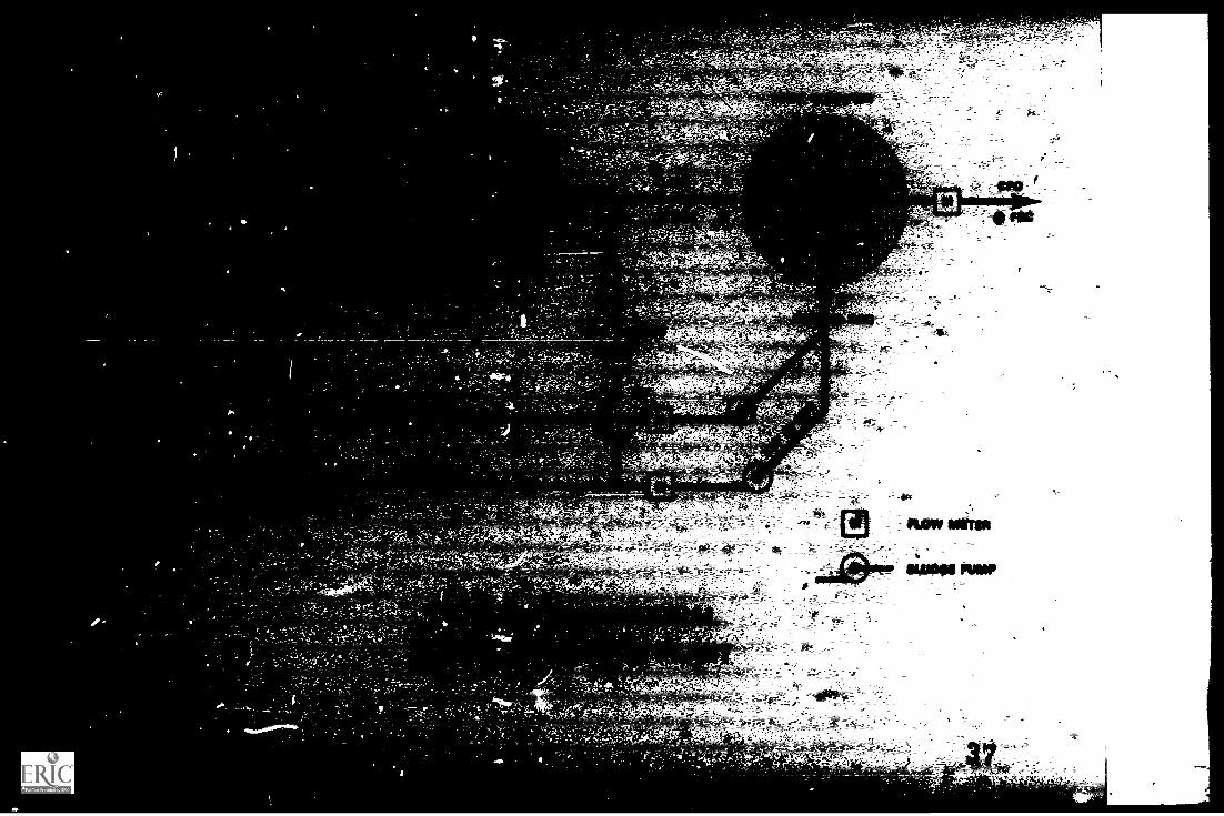
_acme special equipment for operational control testingare uled in the NFIC-C Procedures. Basically a settlometer,centrifuge, turbidimeter, and optical sludge blanket finderare needed. -

The construction of a typical sludge blanket finder isshown in Figure 8. Approximate prices (1973) and types ofcontrol test equipment that have been used by the WasteTreatment Branch are as follows:

Blanket Finder Parts

Site Glass - Part NO. 4045 for 1 1/2" pipe $5.00

Gitz Mfg. Co.1846 South Kilbourn Ave.Chicago, Illinois 60623

tae Schedule 40 aluminum pipe. Tape the tubeevery 0.5 ft. starting at the site glase toeaci-state reading the blanket depth. Fasterreadings may be obtained if distinctive markingsare used at the 5 ft. and 10 ft. points.

Mallory Direct Reading Settlometer

5" dia. x 7" high, 2 liter graduated cyl. $24.00

ecientific Glass Apparatus Co.735 Broad StreetBloomfield, New Jersey 07003

Turbidimeter

Hach Model 2100-A Laboratory Turbidimeter $525.00

Hach Chemical Co.Box 907Ames, Iowa 50010

20

28

Singi IolaToggle Switch

I Volt Batteryw/Screw TerminalsNee Tape or Hose Clampsto Srlf Switch andBattery to Pole)

Distinctive 10ft Marker

11iin. Schedule 40Aluminum Pipe

Wires to Batteryand .Switch ..---....

Distinctive 5ft Marker ---

Place Tape on 0 5ftend 1.0ft IntervalsM Hold Wire and Aidm Determining008

rII.

114m SchOule 40 Aluminum Pipe

(Smaller Size May Be Used onShort Blanket Finders)

Radiator Hose Clamp

...5-- -V x%' Aluminum U-Strap

Threaded114 Pipe Coupling

SEE DETAIL:-40-

Figure 8

SLUDGE BLANKET FINDER

29

Radiator Hose Clamp

Threaded Site Glass Assembly("Gitz" or Equal)

Bulb and SocketFrom Canmbalized Flashlight

Epoxy Cement

Clinical Centrifuge, I.E.C. No. 428

1 - Head, Trunion, 6-place, 15 ml.,I.E.C. No. 221

6 - Shields, Cornell Style, 15 ml.,I.E.C. No. 302

1 Pk - Replacement Thrust Cushions,Rubber, I.E.C. No. 570

International Equipment Co.300 Second Ave.Needham Heights, Mass. 02194

$208.00

$59.00

$31.50/6

$2.40

Centrifuge Tubes - A.P.I.

1 Oz - Kimax No. 45170 $30.00/Dz

Laboratory Ti' er

Interval, electric, 60-minute, withalarm, 2 switches and elapsed timecircuit

Matheson Scientific12101 Centron PlaceCincinnati, Ohio 45246

$35.00

Note: Some of this special testing equipment is notlisterin generalized laboratory equipment catalogs.Manufacturers' catalog numbers are used only to identifytypes of equipment and this does not constitute anendorsement of any manufacturer or supplier.

22

30

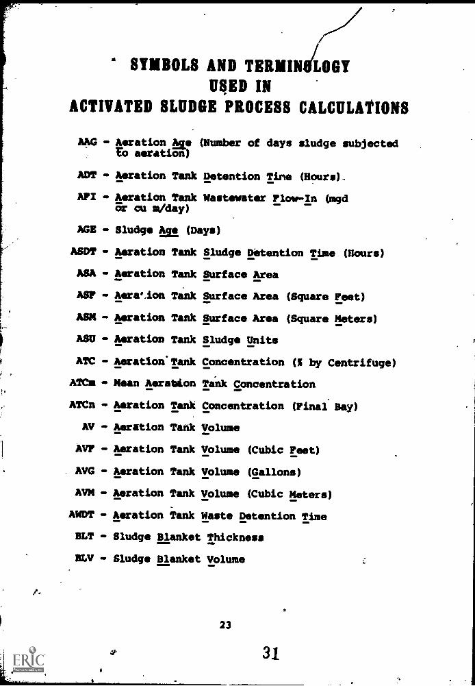
SYMBOLS AND TERMIN/LOGYUSED IN

ACTIVATED SLUDGE PROCESS CALCULATIONS

AAG - Aeration Aqe (Number of days sludge subjectedTO aeration

ADT - Aeration Tank Detention Tine (Hours)-

AFI - Aeration Tank Wastewater Flow-In Owlcr cu m/day)

AGE - Sludge fts (Days)

ASDT - Aeration Tank Sludge Detention Time (Hours)

ASA - Aeration Tank Surface Area

Asr - Aeration Tank Surface Area (Square Feet)

ASK - Aeration Tank Surface Area (Square Meters)

ASU - Aeration Tank Sludge Units

ATC - Aeration-Tank Concentration (% by Centrifuge)

ATC - Mean Aeration Tank Concentration

ATCn - Aeration Tank Concentration (Final Bay)

AV - Aeration Tank Volume

AVF - Aeration Tank Volume (Cubic Feet)

AVG - Aeration Tank Volume (Gallons)

AVM - Aeration Tank Volume (Cubic Meters)

?MDT - Aeration Tank Waste Detention Time

BLT - Sludge Blanket Thickness

BLV - Sludge Blanket Volume

I.

23

31

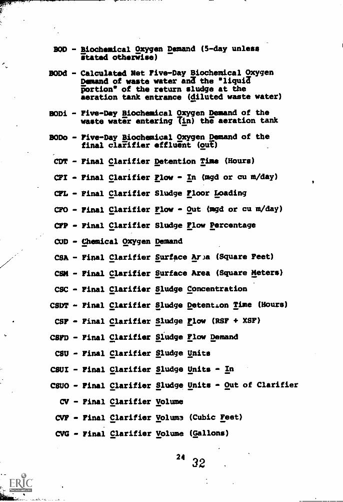
HOD -

BODd -

BODi -

BODo -

CDT -

CFI -

CFL -

CFO -

CFP -

COD -

CSA -

CSM -

CSC -

CSDT -

CSF

CSFD -

CSU

CSUI -

CSUO

CV -

CVF -

CVG

Biochemical Oxygen Demand (5-day unlessstated otherwise)

Calculated Net Five-Day Biochemical OxygenDemand of waste water an the eliquiaportion" of the return sludge at theaeration tank entrance (diluted waste water)

Five-Day Biochemical Oxygen Demand of thewaste water entering Tin) the aeration tank

Five-Day Biochemical Oxygen Demand of thefinal clarifier effluint (out)

Final Clarifier

Final Clarifier

Final Clarifier

Final Clarifier

Final Clarifier

Chemical Oxygen

Final

Final

Final

Final

Final

Final

Final

Final

Final

Final

Final

Final

Clarifier

Clarifier

Clarifier

Clarifier

Clarifier

Clarifier

Clarifier

Clarifier

Clarifier

Clarifier

Clarifier

Clarifier

Detention Time (Hours)

Flow - In (TAO or cu m/day)

Sludge Floor Loading

Flow - Out OW or cu m/day)

Sludge Flow Percentage

Demand

Surface Aria (Square Feet)

Surface Area (Square Meters)

Sludge Concentration

Sludge Detention Time (Hours)

Sludge Flow (RSF + XSF)

Sludge Flow Demand

Sludge Units

Sludge Units - In

Sludge Units - Out of Clarifier

Volume

Volum (Cubic Feet)

Volume (Gallons)

2432

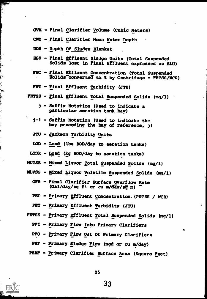
CVM - Final Clarifier Volume (Cubic Meters)

CWD - Final Clarifier Mean Water Depth

DOB - Depth Of Sludge Blanket

ESU - Final Effluent Sludge Units (Total SuspendedSolids lost in Final Effluent expressed as SLU)

FEC - Final Effluent Concentration (Total Suspended&lids convertecT to-% by Centrifuge - FETSS/WCR)

PET - Final Effluent Turbidity (JTU)

FETSS - Final Effluent Total Suspended Solids (ng/1)

j - Suffix Notation (Used to indicate aparticular aeration tank bay)

j -1 - Suffix Notation (Used to indicate thebay preceding the bay of reference, j)

JTU - Jackson Turbidity Units

LOD - Load (lbs BOD/day to aeration tanks)

LODk - Load (kg DOD /day to aeration tanks)

MLVSS - Mixed Liquor Total Suspended Solids (mg/1)

MLVSS - Mixed Liquor Volatile Suspended Solids (ng/1)

OFR - Final Clarifier Surface Overflow Rate(Gal/day/sq ft or cu m/diTY/4 m)

PSC - Primary Effluent Concentrationr(PETSS / WCR)

PET - Primary Effluent Turbidity (JTU)

PETSS - Primary Effluent Total Suspended Solids (ng/1)

PFI - Primary Flow Into Primary Clarifiers

PTO - Primary Flow Out Of Primary Clarifiers

PSF - Primary Sludge Film (mgd or cu m/day)

PSAF - Primary Clarifier Surface Area (Square Feet)

25

33

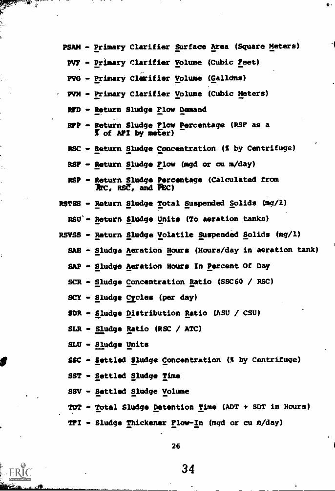
PSAM - Primary Clarifier Surface Area (Square Meters)

PVF - Primary Clarifier Volume (Cubic Feet)

PVG - Primary Clarifier Volume (Galldns)

PVM - Primary Clarifier Volume (Cubic Meters)

RFD - Return Sludge Flow Demand

RFP - Return Sludge Flow Percentage (RSF as a1. of AFI by meEer)

RSC - Return Sludge Concentration (% by Centrifuge)

RSF - Return Sludge Flow (mgd or cu m/day)

RSP - Return Sludge Percentage (Calculated fromRSE, and PEC)

RSTSS - Return Sludge Total Suspended Solids (mg/1)

flSU'- Return Sludge Units (To aeration tanks)

RSVSS - Return Sludge Volatile Suspended Solids (mg/1)

SAH Sludge Aeration Hours (Hours/day in aeration tank)

SAP - Sludge Aeration Hours In Percent Of Day

SCR - Sludge Concentration Ratio (SSC60 / RSC)

SCY - Sludge Excl.. (per day)

SDR - Sludge Distribution Ratio (ASU / CSU)

SLR - Sludge Ratio (RSC / ATC)

SLU - Sludge Units

SSC - Settled Sludge Concentration (% by Centrifuge)

SST - Settled Sludge Time

SSV - Settled Sludge Volume

TDT - Total Sludge Detention Time (ADT + SDT in Hours)

TFI - Sludge Thickener Flow-In (mgd or cu m/day)

26

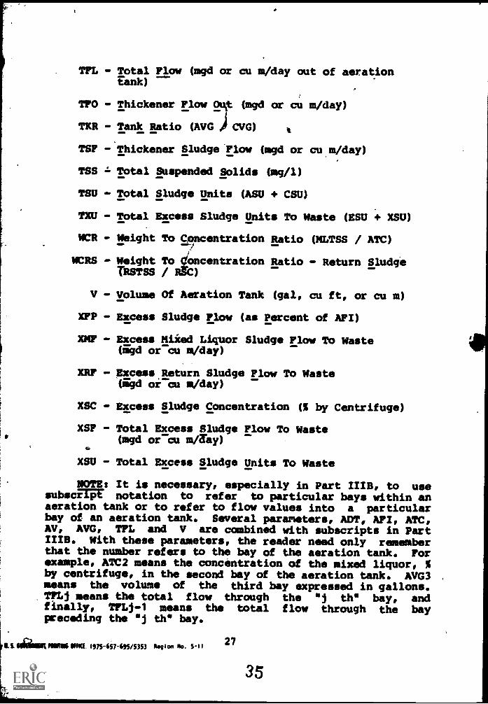
TFL - Total Flow (mgd or cu m/day out of aerationfink)

TFO - Thickener Flow Oust (mgd or cu m/day)

TXR - Tank Ratio (AVG ) CVG)

TSF - Thickener Sludge Flow (mgd or cu m/day)

TSS = Total Suspended Solids (mall)

TSU - Total Sludge Unite (ASU + CSU)

TXU - Total Excess Sludge Unite To Waste (ESU + XSU)

VCR Weight To Concentration Ratio (MLTSS / ATC)

WCRS - Weight Tosecentration Ratio - Return SludgeTRSTSS / )

V - Volume Of Aeration Tank (gal, cu ft, or cu m)

XFP - Excess Sludge Flow (as Percent of AFI)

xmr - Excess ?died Liquor Sludge Flow To Waste(41 or cu m/day)

XRF Excess Return Sludge Flow To Waste(11-0 or cu m/day)

XSC - Excess Sludge Concentration (S by Centrifuge)

XSF - Total Excess Sludge Flow To Waste(mgd or-Cu m/day)

XSU - Total Excess Sludge Units To Waste

NOTE: It is necessary, especially in Part IIIB, to usesubscript notation to refer to particular bays within anaeration tank or to refer to flow values into a particularbay of an aeration tank. Several parameters, AD?, AFI, ATC,AV, AVG, TFL and V are combined with subscripts in PartIIIB. With these parameters, the reader need only rememberthat the number refers to the bay of the aeration tank. Forexample, ATC2 means the concentration of the mixed liquor, %by centrifuge, in the second bay of the aeration tank. AVG3 .

means the volume of the third bay expressed in gallons.11114 means the total flow through the ej the bay, andfinally, TFLj -1 means the total flow through the baypreceding the "j the bay.

1.1111111K MIMS *Fa 1575-657445/5353 Rog Ion No. 5-11 27

35