openness to trade and deforestation atthebrazilian amazon ... · openness to trade and...

1

Openness to Trade and Deforestation at the Brazilian Amazon: A Spatial

Econometric Analysis

Weslem Rodrigues Faria*

Alexandre Nunes de Almeida†

ABSTRACT

The Brazilian Amazon is a large piece of land that hosts only 12% of Brazilian population. Even this low figure and people mostly living in urban areas, the overexploitation of the forest resources driven by economic activities seems to be out-of-control. In the 1970s, abundant government subsidies/incentives for mining, crop and beef production, and gigantic road projects provided infra-structure to the new settlers coming from other parts of the country. Federal and state governments failed in regulating this occupation legally. As a result, for the last decades, frontier regions of Amazon have been a major scene of land conflicts between farmers, squatters, miners, indigenous group and public authorities. Furthermore, from the openness of economy in the 1990s, we also find some evidence that a very attractiveinternational demand for timber, and higher international prices of agricultural commodities are important factors that have been also pushing to more deforestation, through the conversion of forest to new agricultural and pasture areas.

The main objective of this paper is to investigate how international trade has affected the dynamics of deforestation in the Brazilian Amazon. The analysis, at county level, also focuses on the expansion of crop and cattle activities, and other determinants such as gross domestic product, demographic density and roads. To achieve such goal, we combine standard econometrics with the spatial econometrics in order to capture, across the space, the socio -economic interactions among the agents in their interrelated economic system. The data used in this study correspond to a balanced panel for 732 counties from 2000 to 2007 totalizing 6,256 observations.

The main findings suggest that the openness to trade indicator used--export plus import over GDP--goes up, the result is more deforestation. We also find that beef cattle and the production of soybeans, sugarcane and cotton are pushing to more deforestation in the region. The extraction of firewood and timber had both a positive and significant in impact on deforestation, as expected. Moreover, as the GDP goes up, it pushes to more deforestation as well. On the other hand, as the square of GDP goes up indicate less deforestation, supporting, to some extent, the environmental Kuznets Curve hypothesis. The production of non -wood products has a negative impact on deforestation. Unexpected results were also observed such as a negative and no impact on deforestation from population density and road distance.

* PhD candidate in Economics at the University of Sao Paulo ([email protected]).†

Professor at Federal University of São Carlos at Sorocaba ([email protected]).

2

Openness to Trade and Deforestation at the Brazilian Amazon: A Spatial

Econometric Analysis

1. Introduction

Since the 1980s, the importance of tropical forests has been internationally recognized.

Tropical forests are important not only to the global climate regulation but are home to much

of the world’s biodiversity (Barbier, 2001). It is also well known tropical forests are mostly

located in very poor regions in developing nations along the equatorial line, and growing

human activities in these regions are putting an enormous pressure on forest as well as their

ecosystems. Losses of forest cover have been substantial and have occurred so sharply during

the last years. The understanding of this process has become one of the top priorities of any

environmental development agenda, and deserves further investigation.

The Brazilian Amazon, the focus of this paper, is a large piece of land (61% of

national territory) that hosts only 12% of Brazilian population in nine states .1 Even this low

figure and people mostly living in urban areas, the overexploitation of the forest resources

driven by other economic activities seems to be out-of-control. In the 1970s, abundant

government subsidies/incentives for mining, crop and beef production, and gigantic road

projects provided infra-structure to the new settlers coming from other parts of the country

(Mahar, 1989). Federal and state governments failed in regulating this occupation legally;

thereby establishing a common property problem of environmental resource. For the last

decades, frontier regions of Amazon have been a major scene of land conflicts between cattle

ranchers, squatters, miners, indigenous group and public authorities. In addition, more

recently, from the openness of economy in the 1990s, we also find some evidence that the

very attractive demand of international markets for timber, and higher international prices of

agricultural commodities are factors that have been also pushing to more deforestation in the

region (Brandão et al., 2006).

The significant loss of Amazon virgin forest due to cattle ranching and agricultural

activities, poorly defined property rights, road construction and population growth consist of

1

States of Acre, Amapá, Amazonas, Mato Grosso, Rondôni a, Roraima, Tocantins, Pará and parts of Maranhão define what is officially called in Brazil by Legal Amazon.

3

the majors, and direct determinants of the deforestation, that have been extensively studied

(Reis and Guzman, 1992; Pfaff, 1999; Walker et al., 2000; Weinhold and Reis, 2001;

Andersen et al., 2002; Mertens et al., 2002; Margulis, 2003; Chomitz and Thomas, 2003; Pfaff

et al., 2007; Diniz et al., 2009; Araujo et al., 2009; Rivero et al., 2009; Barona et al., 2010).

However, to our best knowledge, there are very few studies that investigate the relationship

between deforestation and openness to trade in developing countries .

The objective of this paper is to give a special attention how international trade has

affected the dynamics of deforestation in the Brazilian Amazon. Moreover, we also focus on

the expansion of agricultural and cattle activities. The analysis, at county level, will also

include other determinants commonly used for this kind of analysis such as gross domestic

product, demographic density and road distance. To achieve such goal, we combine standard

econometrics with the spatial econometrics in order to capture, across the space, the socio-

economic interactions among the agents in their interrelated economic system in the Amazon

region.

2. Theoretical Background and Literature Review

In the literature, few contributions have directly prioritized degradation of renewable natural

resources and international trade. Generally speaking, the punch line of these studies is that if

property-rights of the environmental resource are ill-defined, then trade between two countries

does not make both better off in terms of resources allocations and income, as usually

defended by the international trade’s proponents. The theory behind this argument relies on

the works of Chichilnisky (1994), Brander and Taylor (1996), and Ferreira (2004).

Chichilnisky, for example, assumes a two-country economy, where the south country and

property rights of natural resource are ill-defined. It exports environmental intensive goods .

She shows that although trade is able to equalize output and factor prices between north and

south, it does not improve resource allocation in the south country. Since the south is poor and

owns a subsistencesector (labor), tax policies on the use of the resource that would decrease

the price of the resource is a reason to lead to even more extraction (overproduction) of the

common property. In the Brazilian Amazon, since the 1970s, outside of colonization’s

projects, along the roads, public land and unused private land have been occupied at minimum

4

(no) cost at all. Further evidence suggests that most landholders do not have legal titles or

have fake titles of their land (Araujo et al., 2009).

Ferreira (2004) also supports the lack of property rights by south leads to more

overexploitation. She built a model that exploits the difference between the marginal and

average product of labor assuming diminishing returns between a south and a north country.

Both share s imilar technological levels , two goods (manufacturing and resource) and two

factors endowments (stock of natural resource and labor). The main reason for trade is the

difference in property rights over natural resources between countries, and not the difference

in the resource abundance. Thus, increases in autarky prices brought by trade shift up the

value of marginal product and the value of average product curves inducing labor migration

from manufacturing sector to the harvest sector. She concludes that even the south becomes a

net exporter, it experiences losses from trade. In addition, the elimination of trade distortions

enlarges the effects of property rights distortions which also damage the south country.

Brander and Taylor (1995) analyze an open small country economy. Natural resource--

fishing or forest--is abundant, and property rights are not enforced. Considering a Ricardian

economy, the authors show that under free trade, the small country, even with comparative

advantage in natural resource good, may still suffer losses in economic terms and the use of

natural resources .

Some of the conclusions above have been confirmed empirically. Ferreira (2004)

analyzed data of 92 countries for 1961-1994 and found that the usual openness indicator

export plus import over GDP is a significant predictor of deforestation but only when

interacting with institution factors such as risk of expropriation, corruption and bureaucracy.

Lopez and Galinato (2005), using household surveys for Brazil, Indonesia, Malaysia and

Philippines, found that the net impact of trade openness was small and of different directions

for the four countries between 1980 and 1999. For example, if openness to trade increases

forest cover in Brazil and Philippines , it decreases forest cover in Indonesia and Malaysia.

Using data of 1989 for Ghana, Lopez (1997) found the reduction of tariff protection

and export taxes implied in losses of biomass (natural fertilizer used by farmers) of 2.5-4%,

and the overexploitation of biomass through a more than optimal level of land cultivated due

to tariff reductions had a small impact on national income. More recently, Arcand et al. (2008)

show theoretically that depreciation of the real exchange rate and weaker institutions push to

5

more deforestation in developing countries. In an empirical application, they did not reject any

of the hypotheses above on annual data for 101 countries from 1961 to 1988.

3. Data

The data used in this study correspond to a balanced panel for 732 counties from 2000 to 2007

totalizing 6,256 observations. These counties are part of PRODES (Programa de

Monitoramento da Floresta Amazônica Brasileira por Satelite) project funded by the

Brazilian Government to monitor the level of deforestation in the Brazilian Amazon. The

National Institute of Spatial Research (INPE) collects and publishes regularly geo-referenced

annual rate of deforestation of high quality for all 732 counties that are constitute the Legal

Amazon. Other variables used are also from secondary sources , mostly from also other

government institutions among them: Ministry of Development, Industry and Trade, the

Brazilian Statistical National Institute (IBGE) and the Institute of Applied Economic Research

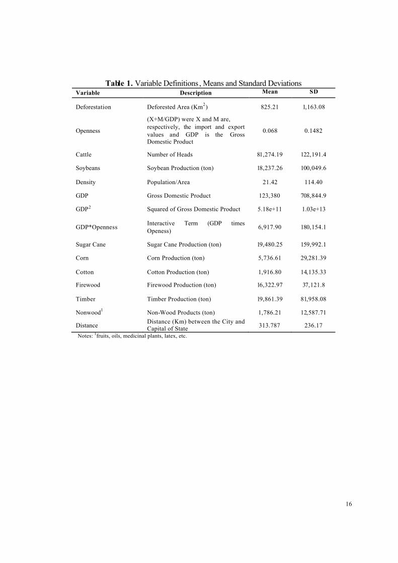
(IPEA).2 Table 1 shows the description of each variable used as well as its means and standard

deviation.

4. Methodology

4.1 Tests of Spatial Autocorrelation

As proposed, the following strategy adopted is to combine the standard econometrics with the

spatial econometrics. But, firstly, what is called by Exploratory Spatial Data Analysis (ESDA)

is needed. The ESDA defines a spatial weight matrix such that it will provide us a contiguous

criterion among the spatial units , i.e., counties (Anselin, 1988). This study adopts the k -

nearest neighbors as contiguous criterion, which has widely used for other studies (Pace and

Barry, 1997; Pinkse and Slade, 1998; Baller et al., 2001; Le Gallo and Ertur, 2003).

2 Some variables had missing observations regarding some municipalities in a few years of the study’s period. In order to overcome this problem, geographically weighted estimates were made for generating those observations. The procedure involves the estimation by the OLS procedure with the following specification: � = � + �� +�� + �� + �� + �� + �� + �, where x and y represent latitude and longitude of the centroid of each

spatial unit; m refers to the vector o f vari ables used in econometric model to determine the dynamics of the deforestation that had missing observations; β

iis the vector of coefficients to be estimated for each i, where i

indicates the relevant variable with missing observations and; ε the error term.

6

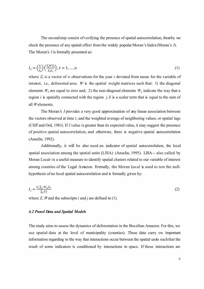
The second step consist of verifying the presence of spatial autocorrelation, thereby we

check the presence of any spatial effect from the widely popular Moran’s Index (Moran’s I).

The Moran’s I is formally presented as:

�� = ��

��

� ��

′ ��

��′ ��

� , � = 1, … , � (1)

where Zt is a vector of n observations for the year t deviated from mean for the variable of

interest, i.e., deforested area. W is the spatial weight matrices such that: 1) the diagonal

elements Wii are equal to zero and; 2) the non-diagonal elements Wij indicate the way that a

region i is spatially connected with the region j. S is a scalar term that is equal to the sum of

all Welements.

The Moran’s I provides a very good approximation of any linear association between

the vectors observed at time t, and the weighted average of neighboring values, or spatial lags

(Cliff and Ord, 1981). If I value is greater than its expected value, it may suggest the presence

of positive spatial autocorrelation, and otherwise, there is negative spatial autocorrelation

(Anselin, 1992).

Additionally, it will be also used an indicator of spatial autocorrelation, the local

spatial association among the spatial units (LISA) (Anselin, 1995). LISA-- also called by

Moran Local--is a useful measure to identify spatial clusters related to our variable of interest

among counties of the Legal Amazon. Formally, the Moran Local is used to test the null-

hypothesis of no local spatial autocorrelation and is formally given by:

�� =�� ∑ ��

∑ ��

� (2)

where Z, Wand the subscripts i and j are defined in (1).

4.2 Panel Data and Spatial Models

The study aims to assess the dynamics of deforestation in the Brazilian Amazon. For this, we

use spatial data at the level of municipality (counties). These data carry on important

information regarding to the way that interactions occur between the spatial units such that the

result of some indicators is conditioned by interactions in space. If these interactions are

7

significant in such way that the result in a spatial unit affects the outcome in neighboring

spatial units, then the data are spatially auto correlated. The presence of spatial autocorrelation

violates the underlying assumption of independence of observations of linear regression

models. The dependence of observations in space arises from the existence of a correlation

between the data of the dependent variable or error term with data from neighboring spatial

units. Thus, a common way to test the spatial dependence is to verify the presence of spatial

autocorrelation. In this study, we use the Moran's I test to detect spatial autocorrelation, as

explained above, and therefore to verify the presence of spatial dependence.

The presence of spatial dependence, according to Anselin (1988) and Anselin and Bera

(1998), can make the OLS estimators inconsistent and/or inefficient. However, according

Anselin (1995), spatial dependence can be incorporated into linear regression models in two

ways. First, through the construction of new variables, both for the dependent variable and for

the explanatory variables and error terms of the model. These new variables incorporate

spatial dependence as a weighted average of the values of the neighbors. Second, by using

spatial autoregressive error terms. This study followed the first suggestion, adding variables to

the model to mitigate the consequences of spatial dependence.

It is well known that one of the main advantages of using panel data is to control for

observed and also for unobserved characteristics (Baltagi, 1995). In such cases, fixed effects

and random effects specifications are the most commonly models used in applied work.

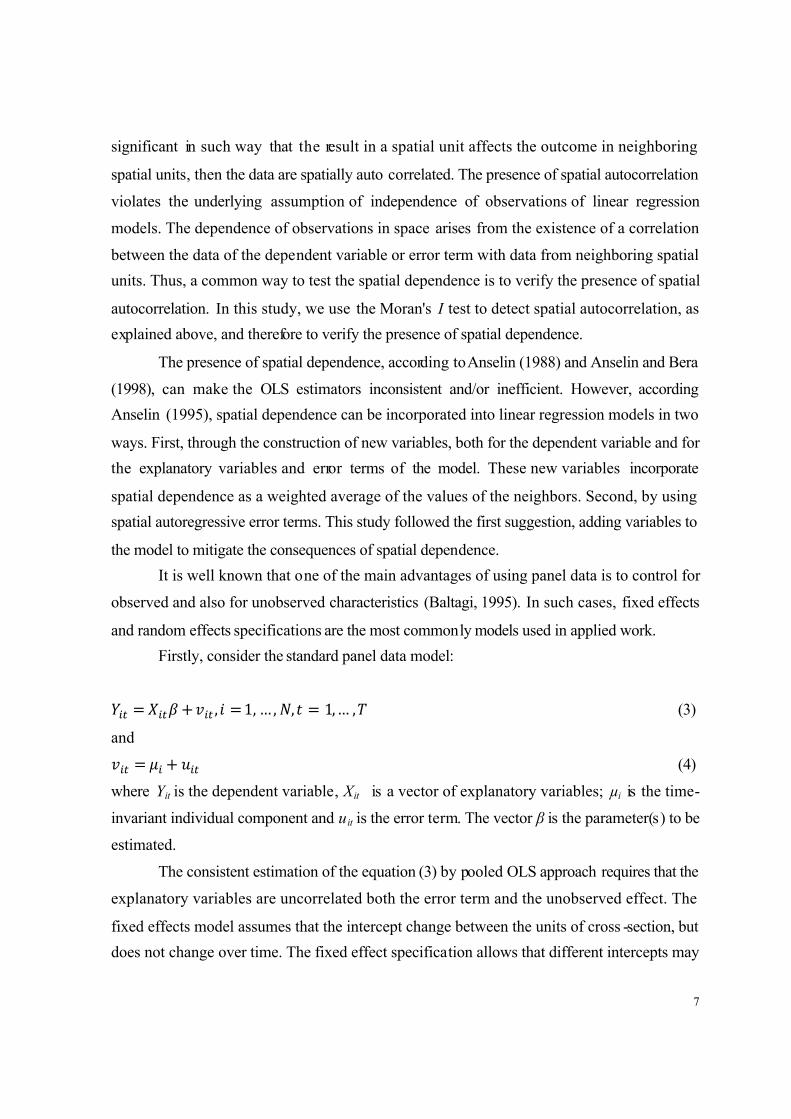
Firstly, consider the standard panel data model:

�� = �� + �� , � = 1, … , �, � = 1, … , � (3)

and

�� = �� + �� (4)

where Yit is the dependent variable, Xit is a vector of explanatory variables; µi is the time-

invariant individual component and u it is the error term. The vector β is the parameter(s) to be

estimated.

The consistent estimation of the equation (3) by pooled OLS approach requires that the

explanatory variables are uncorrelated both the error term and the unobserved effect. The

fixed effects model assumes that the intercept change between the units of cross -section, but

does not change over time. The fixed effect specification allows that different intercepts may

8

to capture all the differences between the units of cross-sections. The random effects model

assumes that the behavior of both the units of cross-section and the time is unknown.

Therefore, the behavior of these units of cross-section and the time can be represented in the

form of a random variable, and the heterogeneity is treated as part of the error term.

Moreover, the random effects model present the futher assumption that unobserved term is

uncorrelated with the explanatory variables (Johnston and Dinardo, 1997).

However, under the presence of spatial autocorrelation, the adoption of these

procedures is not enough, and some extensions specific for panel data have been developed

(Elhorst, 2003). It is worth mentioning that such models to be presented attend the same

properties as the traditional panel data ones, being that the major difference consists of only

adding more explanatory variables that take into account the spatial effect. Nevertheless, no

special treatment is given to residual values of these regressions. We will provide more details

below.

Now, consider the following models that take into account the spatial effect (Anselin

and Bera, 1998; Anselin, 2001; Anselin, 2003, Carvalho, 2008):

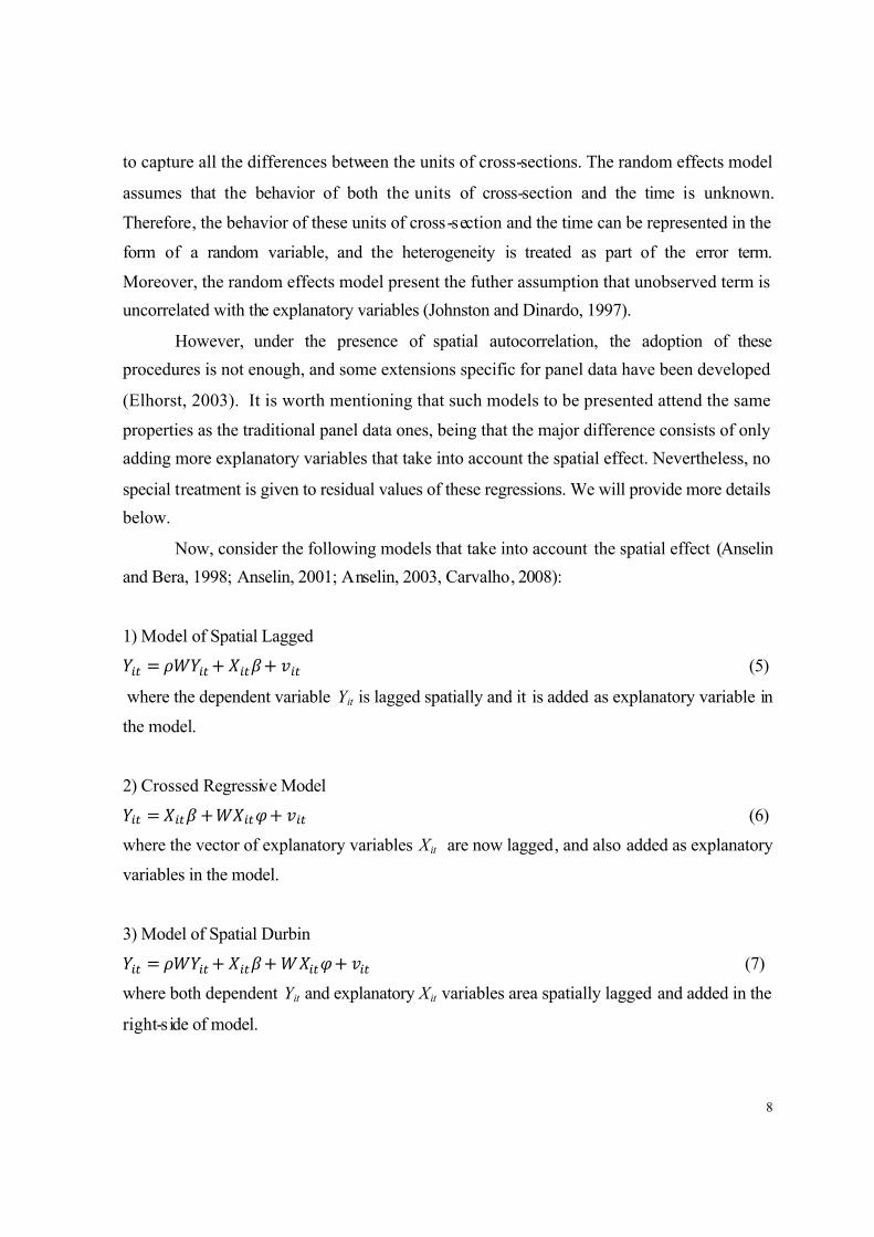
1) Model of Spatial Lagged

�� = �� + ��+ �� (5)

where the dependent variable Yit is lagged spatially and it is added as explanatory variable in

the model.

2) Crossed Regressive Model

�� = �� + �� + �� (6)

where the vector of explanatory variables Xit are now lagged, and also added as explanatory

variables in the model.

3) Model of Spatial Durbin

�� = �� + ��+ �� + �� (7)

where both dependent Yit and explanatory Xit variables area spatially lagged and added in the

right-side of model.

9

The equations (5) and (7) are very unusual; because they have both the dependent

variable as explanatory variable. If the value of this variable for a county is simultaneously

determined by its neighbors, then the equilibrium result will occur in a function of some

existing spatial or social interaction process between both locations (Anselin et al., 2008).

This might be justified either in theoretical or in practical terms because the deforestation

could also be a phenomenon that occurs only as an interactive factor in the space being

determined according to the availability and accessibility of the resource by the economic

agents involved. Such models are gaining enormous popularity in the literature to evaluate

similar situations in which social or spatial interaction might exist (see Brueckner, 2003 and

Glaeser et al., 2002).

The models (5)-(7) produce consistent and non-biased estimates since such models

represent alternatives whose purpose is to take in account the spatial effect of data. However,

Anselin et al. (2008) point out that the estimation of these models under the presence of fixed

or random effects from standard econometric packages might still suffer losses of efficiency

as we shall see ahead.

The procedures to be executed can be summarized as follow:

Step 1. Define a spatial weight matrix and test the presence of spatial autocorrelation at global

and local level.

Step 2. Run fixed and random effects models and get the residuals.

Step 3. Use the residuals to check for spatial autocorrelation.

Step 4. Run panel data models that take in account the spatial autocorrelation and get the

residuals.

Step 5. Perform the spatial autocorrelation tests again in the residuals generated from models

in step 4.

5. Results

Before moving to the heart of the analysis, we need to test the presence of spatial

autocorrelation in the data. As describe above, Moran’s I--global and local--is calculated for

the variable of interest, the deforested area (Km2) for the 732 counties of Legal Amazon from

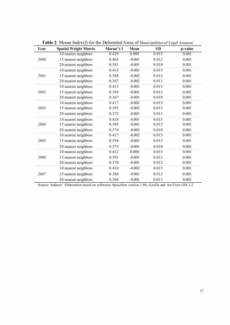
2000 to 2007. The results are shown in Table 2. For all years analyzed, we rejected at the 1%

10

of statistical level the hypothesis there is no global spatial autocorrelation, suggesting that

spatial components have to be considered in the regression model.3 Otherwise, biased and

inefficient estimates would be observed. The coefficients are positive indicating global spatial

autocorrelation positive. The spatial weight matrix of 10 nearest neighbors presented spatial

autocorrelation coefficients more significant than others in all the years analyzed. Therefore,

the following steps were taken based on this matrix (Table 2).

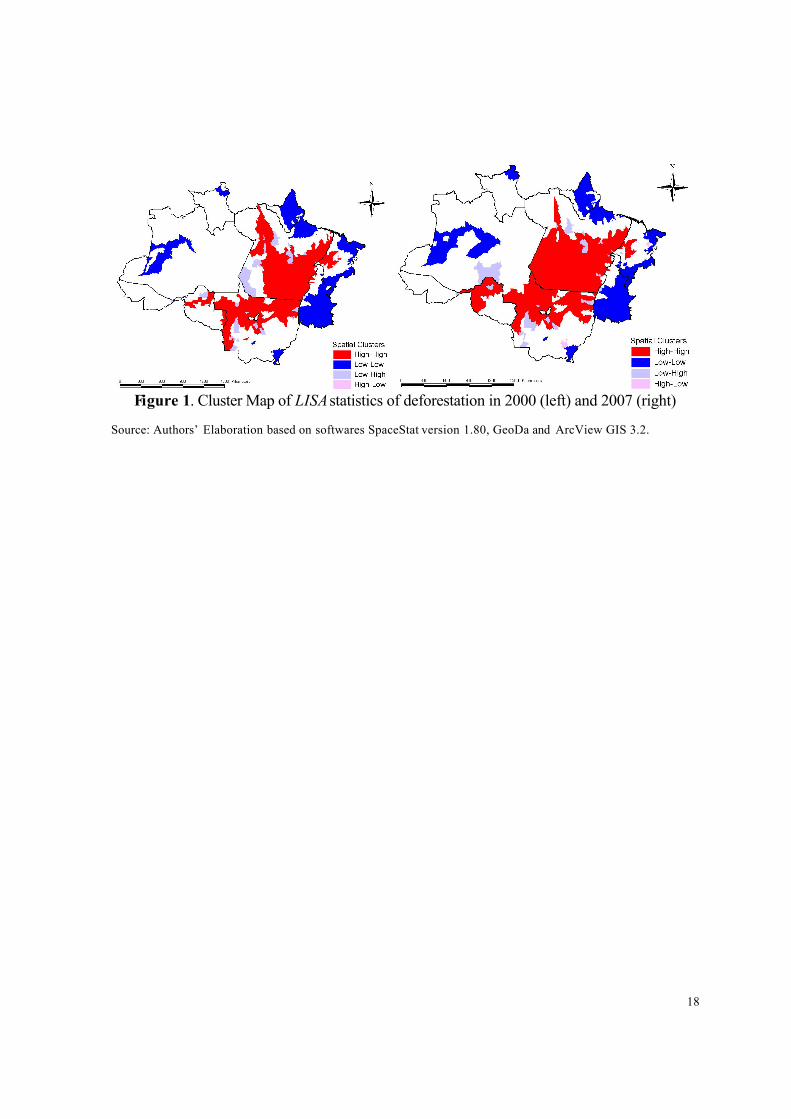
Figure 1 illustrates the LISA statistics (Local Moran) of deforestation for 2000 and

2007. The objective is to show maps of significant clusters such that there could also have

significant spatial autocorrelation at local level. The LISA indicator provides the statistical

inference about the patterns of spatial autocorrelation at local level. Therefore, such indicator

shows only the significant clusters. We can highlight two predominant regimes in both years:

i) High-High: a cluster that covers a large part of Pará state and North of Mato Grosso state.

This suggests that counties with high rates of deforestation are surrounded by counties that

also present high rates of deforestation; ii) Low-Low: a cluster that represents parts of

Amazonas state and parts of Pará state, and almost all regions of Amapá and Tocantins states.

From 2000 to 2007, the High-High cluster becomes more important with increasing extent of

coverage, mainly in the states of Pará and Rondônia. Another regime that appears is the Low-

High, especially in the state of Pará and Mato Grosso. This regime indicates the spatial units

that have low rates of deforestation, but surrounded by spatial units that have high rates of

deforestation.

Both statistics , Moran’s I and LISA clearly lead to the evidence that there is the

presence of some spatiality in the data for deforested areas of Legal Amazon. However, such

results are not still sufficient to verify if this problem would be also observed during the

econometric results.

The second step, thus, is to verify if there is spatial autocorrelation among the

determinants that are omitted during the econometric estimation. This is easily done by

performing spatial correlation tests in the residuals of the regressions. Firstly, we proceed our

analysis running a fixed/random effect models without correcting to any spatial

autocorrelation whatsoever. The results of pooled, fixed and random effects are displayed in

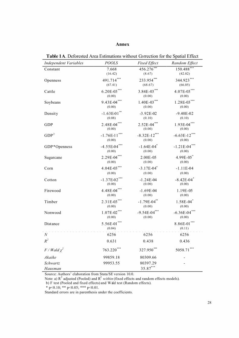
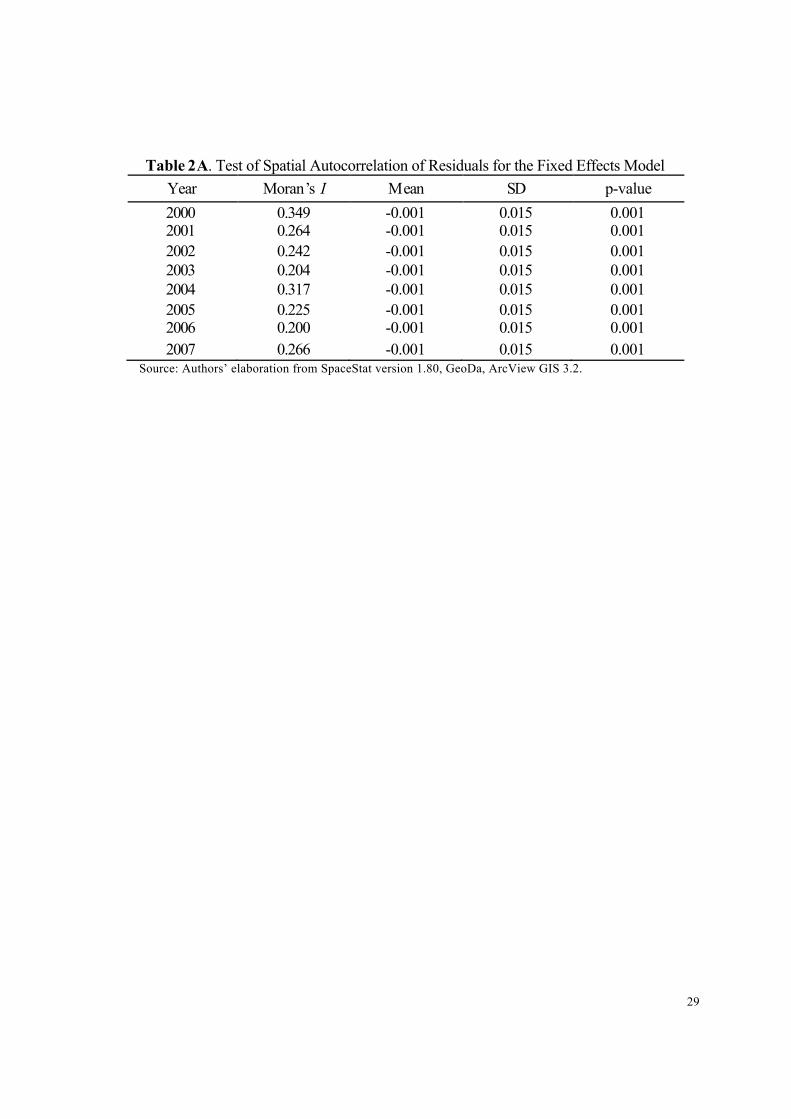
Table 1A (Annex). The Hausman test indicates that the fixed effects model is more suitable to 3

A randomized procedure of Moran Indexes was used to run this test (details about the procedure can be found in Anselin, 2005).

11

our data than the random effects model. Also, the Moran’s I test performed for the vector of

residuals from the fixed effects model does reject the hypothesis of the presence of no spatial

autocorrelation at 1% level of significance.4 Some of our variables of interest, openness to

trade and areas of agricultural commodities , their coefficients had expected signs and were

statistically significant. However, as mentioned previously, not taking into account any

spatial effects leads to inappropriate analysis about the dynamic of deforestation at Amazon

and should not be used as policy decisions.

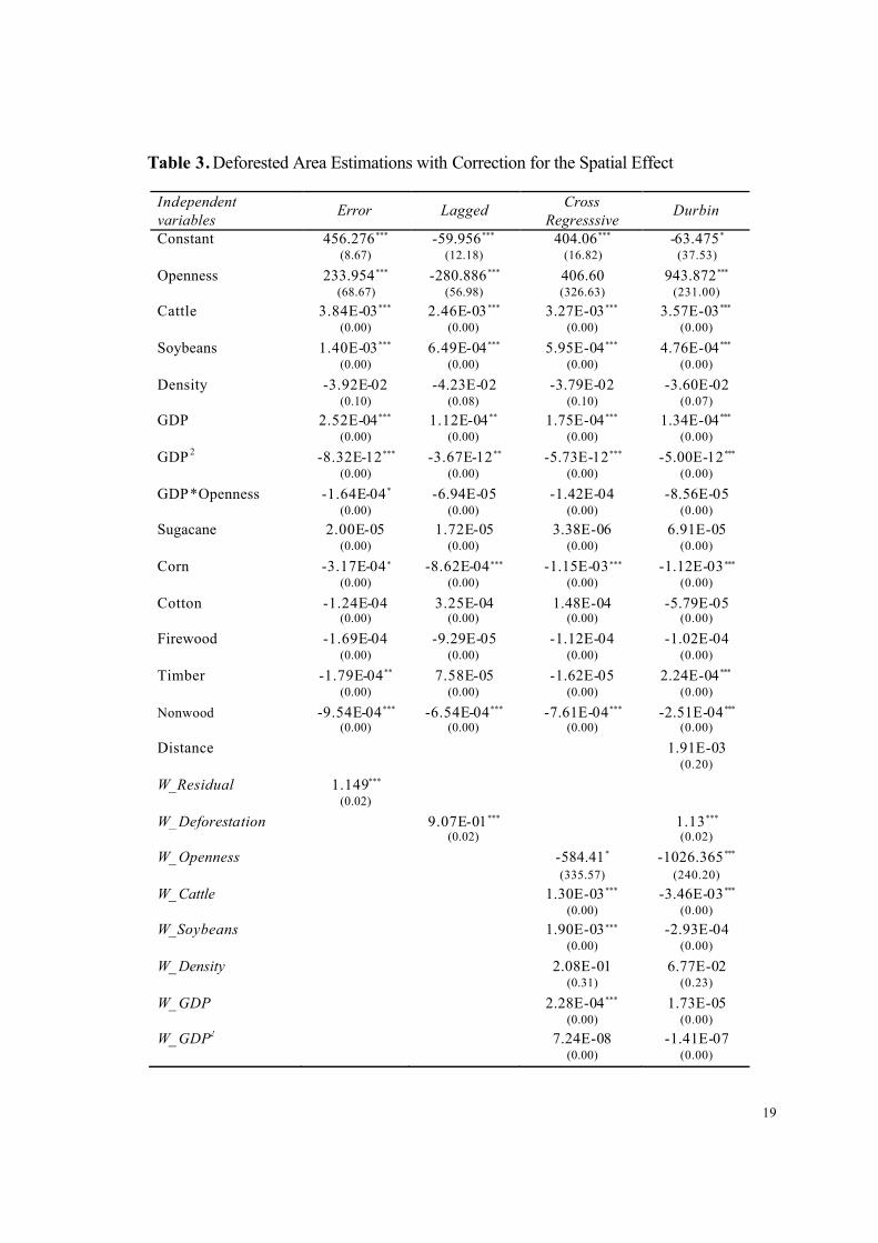
The next step is to estimate specific models that capture spatial effects. Three models

proposed (equations (5), (6) e (7)) are estimated plus a fourth model, the Spatial Error Model

(Spatial Autoregressive Model – SAR). Anselin (2008) shows that when SAR model is

utilized whether for panel data or cross -section, it is able to produce efficient, unbiased and

consistent estimators. This model is estimated in two stages and is given by:

�� = �� + �� (8)

and

�� = �� + �� (9)

where the predicted �� term from (9) is spatially lagged and used as explanatory variable in

the original model (8). The results of this model produce identical estimates as the ones

observed in the ordinary fixed effects model, although is possible to show that the statistical

inference of SAR models might still be compromised. In such case, a specific software (or

procedure) to deal with spatial effect at panel data level is recommended.5 To allow correct

estimates regarding to standard deviation of SAR, alternative models can be found in Baltagi

and Li (2006), Baltagi et al. (2006) and Baltagi et al. (2007).

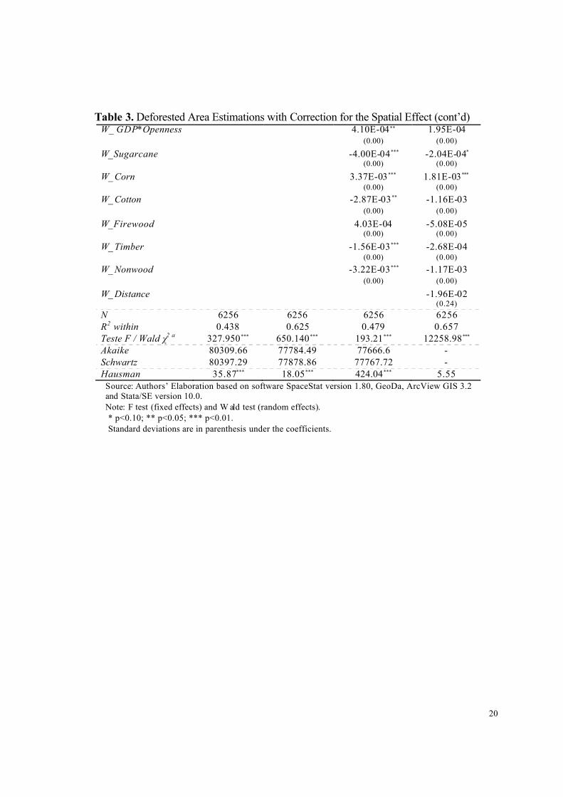
The results presented in the Table 3 are good, but still not sufficient to infer that the

spatial effect was controlled. It is still necessary to verify if there is any spatial effect in the

residuals generated by these regressions.6 The Moran’s I test performed in the residual vectors

showed that the spatial effect still persists and has to be to take into account in some different

4

Table 2A (annex) presents the test of spatial autocorrelation for the residuals from the model what was chosen, the fixed effects model.5 Currently there is no software to perform spatial econometric analysis in the context of panel data. Routines were developed by independent researchers (e.g., James P. LeSage) that can be implemented in MATLAB or R. 6

The Table 3 displays the results for the four models proposed. A Hausman test (Ho: FE versus RE) was performed for each.

12

way.7 Thus, Anselin (1992) suggests two procedures: 1) Create spatial regimes that consider

distinct situations related to the variable of interest. Thus, the estimation will be executed

following distinct groups of observations; 2) Create dummies to control any effects steaming

from spatial outliers. For convenience purposes, we opted for the second option to mitigate

the still present spatial effects.

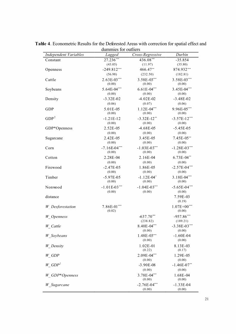
The Table 4 shows the results of three models (Lagged, Cross Regressive and Durbin)

with dummies for spatial outliers. From previous results (Table 3), the fixed effects

specification was kept for the Lagged and Cross -Regressive models and a random effects

model was estimated for the Durbin model. It is well worth mentioning again the adoption of

these different models by using the conventional panel data structure, according to the

literature, is not still a strict spatial econometric procedure such that more information

regarding to neighboring effect would be required. Thus, the inclusion of spatial lagged

explanatory variables is an attempt to reduce possible shortcomings of omitting the spatiality

of data that is still present. The inclusion of dummies is , again, justified to reduce the still

potential spatial effect and obtain more reliable estimates regarding to the parameters. The

variable DUMMY_S represent spatial units with value equal or superior than 2.5 standard

deviations and the variable DUMMY_I represents spatial units with value equal or inferior

than -2.5 standard deviations.

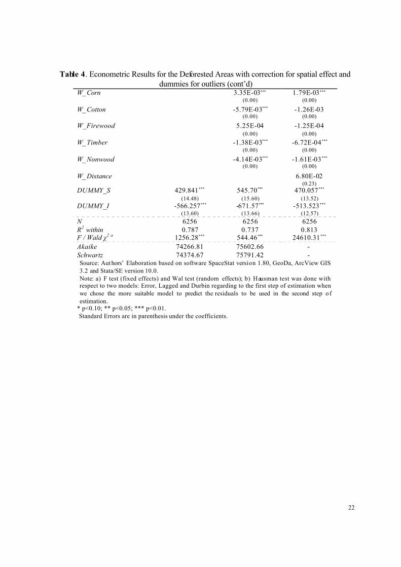
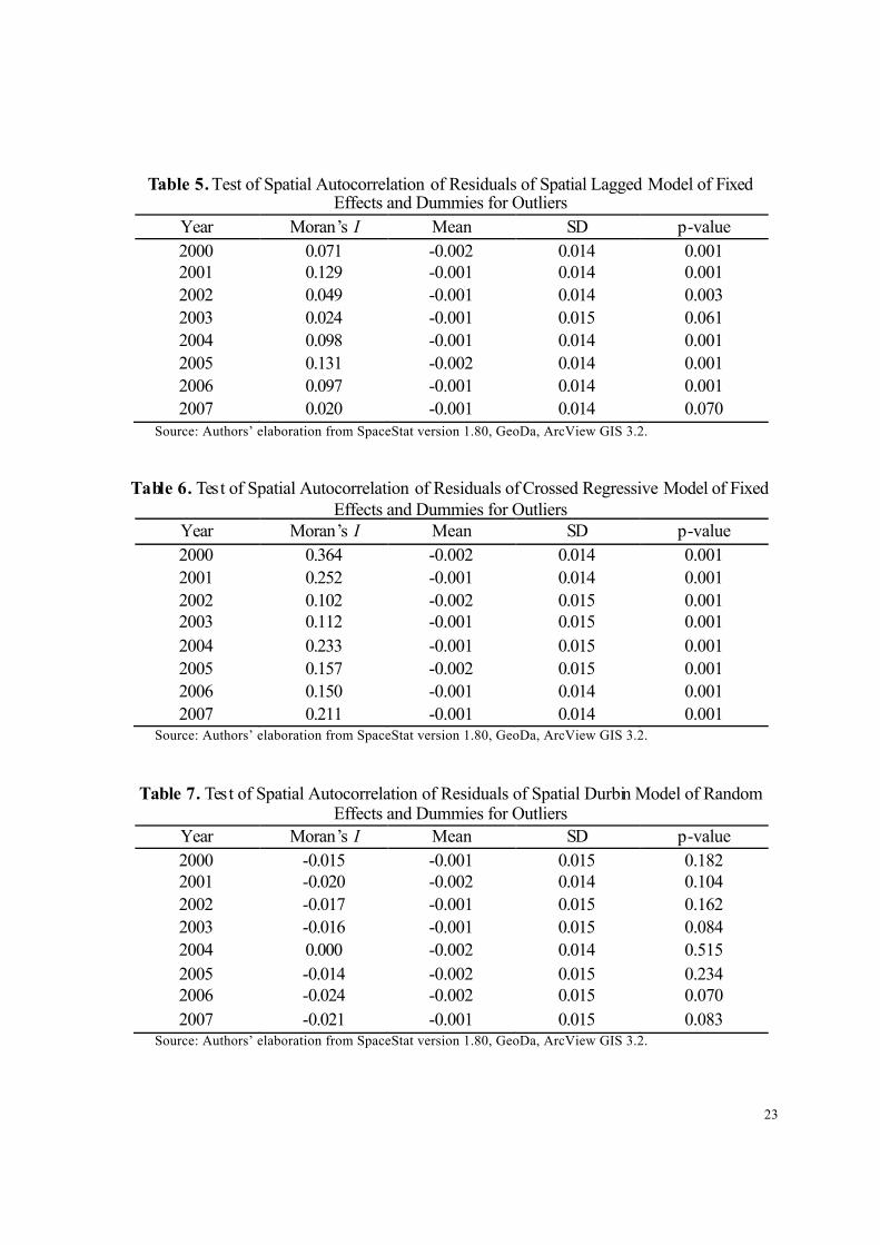
Spatial autocorrelation tests were performed in the residual for the three models

estimated above (Tables 5-7). The tests indicated that the Durbin model was more suitable to

explain the dynamic of deforestation at Amazon. The hypothesis that there is no spatial

autocorrelation was not rejected at minimum statistical level of 7% (Table 7). The results of

Durbin model presented most regression coefficients were not only significant at 1% level but

showed expected signs. This result indicates that the spatial effect is present so that the

average level of deforestation and the average values of the explanatory variables of the

neighbors together to influence deforestation rate in each spatial unit. This result shows the

existence of spatial interaction with relation to deforestation. This means that the spillover

effects both of deforestation and other activities in neighboring spatial units are important in

explaining deforestation in each spatial unit.

7

The results of these tests were omitted in order not to further extend the work.

13

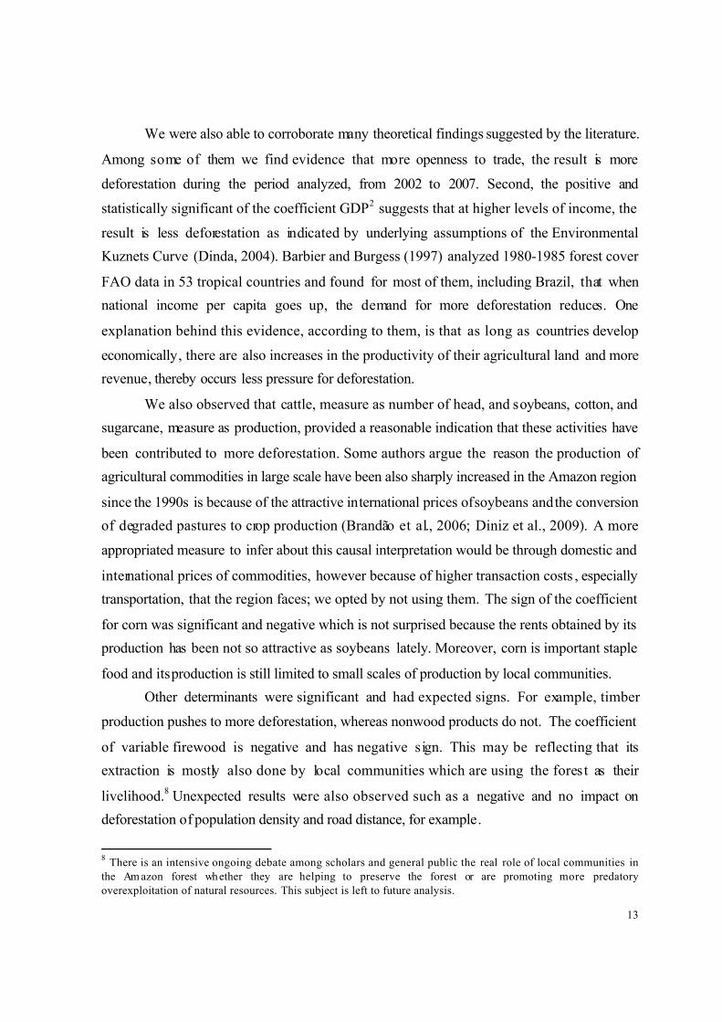
We were also able to corroborate many theoretical findings suggested by the literature.

Among some of them we find evidence that more openness to trade, the result is more

deforestation during the period analyzed, from 2002 to 2007. Second, the positive and

statistically significant of the coefficient GDP2 suggests that at higher levels of income, the

result is less deforestation as indicated by underlying assumptions of the Environmental

Kuznets Curve (Dinda, 2004). Barbier and Burgess (1997) analyzed 1980-1985 forest cover

FAO data in 53 tropical countries and found for most of them, including Brazil, that when

national income per capita goes up, the demand for more deforestation reduces. One

explanation behind this evidence, according to them, is that as long as countries develop

economically, there are also increases in the productivity of their agricultural land and more

revenue, thereby occurs less pressure for deforestation.

We also observed that cattle, measure as number of head, and soybeans, cotton, and

sugarcane, measure as production, provided a reasonable indication that these activities have

been contributed to more deforestation. Some authors argue the reason the production of

agricultural commodities in large scale have been also sharply increased in the Amazon region

since the 1990s is because of the attractive international prices ofsoybeans and the conversion

of degraded pastures to crop production (Brandão et al., 2006; Diniz et al., 2009). A more

appropriated measure to infer about this causal interpretation would be through domestic and

international prices of commodities, however because of higher transaction costs , especially

transportation, that the region faces; we opted by not using them. The sign of the coefficient

for corn was significant and negative which is not surprised because the rents obtained by its

production has been not so attractive as soybeans lately. Moreover, corn is important staple

food and its production is still limited to small scales of production by local communities.

Other determinants were significant and had expected signs. For example, timber

production pushes to more deforestation, whereas nonwood products do not. The coefficient

of variable firewood is negative and has negative sign. This may be reflecting that its

extraction is mostly also done by local communities which are using the forest as their

livelihood.8 Unexpected results were also observed such as a negative and no impact on

deforestation of population density and road distance, for example.

8

There is an intensive ongoing debate among scholars and general public the real role of local communities in the Am azon forest whether they are helping to preserve the forest or are promoting more predatory overexploitation of natural resources. This subject is left to future analysis.

14

Many spatially lagged variables were statistically significant which clearly provide

evidence that the neighboring effect is important for the results. In these cases, there are

significant spillover effects of some other spatial units. For example, the coefficient of the

variable W_Deforestation indicates that the effect of deforestation on a spatial unit tends to be

positive about the situation of deforestation of each of its neighbors. This is expected since the

deforestation activity expands in space in such way as the amount of forest becomes scarce in

the spatial reference of unit, in a form of contagion.

The coefficient of the variables Openness and Cattle spatially lagged exhibit negative

coefficients indicating that situations of greater openness to trade and expansion of livestock

in neighboring spatial units affect negatively the deforestation in the spatial reference unit.

This means that despite the increase in openness to trade and livestock activities in a spatial

unit contributes to the increase in its deforestation, if it occurs in neighboring spatial units, the

effect is to reduce its deforestation. Such result is an explanation, for example, that these

activities might compete to be located in the space. As a result, if activities focused on

openness to trade and/or related to cattle are located in a municipality, and thereby having

positive effects on its own deforestation, it means that such activities have ceased to be

located in other municipality, excluding greater possibilities of deforestation in this location.

6. Concluding Remarks

The main objective of this paper was to investigate how international trade has affected the

dynamics of deforestation in the Brazilian Amazon. The analysis also focuses on the

expansion of crop and cattle activities, and other determinants such as gross domestic product,

demographic density and roads. The combination between standard econometrics and spatial

econometrics intended to capture, across the space, the socio-economic interactions among the

agents.

The main findings were interesting and allowed us to corroborate some of theoretical

findings from the literature, and not well documented. For example, as long as counties are

more opened to international trade, the result is more deforestation. In fact, is not surprised

that public authorities are failing to contend the overexploitation of natural resources,

especially timber, to attend domestic and mainly international markets. Furthermore, poverty,

15

land conflicts, illegal logging and corruption are very old chronicle problems in the region

(Araujo et al., 2009) and have to be tackled by more efforts than only political will.

Other determinants such as the expansion of beef cattle and the production of

soybeans, sugarcane and cotton are important determinants that are pushing to more

deforestation in the region. Some argue that increases in productivity for these economic

activities through technological change could help alleviating substantially the pressure on

natural resources (Brandão et al., 2006). Also, we found important evidence that when the

square of GDP goes up, the result is less deforestation, supporting, to some extent, the

environmental Kuznets Curve hypothesis.

Finally, from the results, we found more support that some of development strategies

to be undertaken in region, in order to alleviate poverty, while also benefiting the

environment, should be able to increase income through other economic activities, and

increases in agricultural productivity, rather than the ones that promote the overexploitation of

natural resources.

16

Table 1. Variable Definitions , Means and Standard DeviationsVariable Description Mean SD

Deforestation Deforested Area (Km2) 825.21 1,163.08

Openness

(X+M/GDP) were X and M are,respectively, the import and export values and GDP is the Gross Domestic Product

0.068 0.1482

Cattle Number of Heads 81,274.19 122,191.4

Soybeans Soybean Production (ton) 18,237.26 100,049.6

Density Population/Area 21.42 114.40

GDP Gross Domestic Product 123,380 708,844.9

GDP2 Squared of Gross Domestic Product 5.18e+11 1.03e+13

GDP*OpennessInteractive Term (GDP times Openess)

6,917.90 180,154.1

Sugar Cane Sugar Cane Production (ton) 19,480.25 159,992.1

Corn Corn Production (ton) 5,736.61 29,281.39

Cotton Cotton Production (ton) 1,916.80 14,135.33

Firewood Firewood Production (ton) 16,322.97 37,121.8

Timber Timber Production (ton) 19,861.39 81,958.08

Nonwood1

Non-Wood Products (ton) 1,786.21 12,587.71

DistanceDistance (Km) between the City and Capital of State

313.787 236.17 Notes: 1fruits, oils, medicinal plants, latex, etc.

17

Table 2. Moran Index (I) for the Deforested Areas of Municipalities of Legal Amazon

Year Spatial Weight Matrix Moran’s I Mean SD p-value

2000

10 nearest neighbors 0.429 0.000 0.015 0.001

15 nearest neighbors 0.403 -0.001 0.012 0.001


2001




2002




2003




200410 nearest neighbors 0.418 -0.001 0.015 0.00115 nearest neighbors 0.395 -0.001 0.012 0.001


2005




2006

10 nearest neighbors 0.412 0.000 0.015 0.001



2007




Source: Authors’ Elaboration based on softwares SpaceStat version 1.80, GeoDa and ArcView GIS 3.2.

18

Figure 1. Cluster Map of LISAstatistics of deforestation in 2000 (left) and 2007 (right)

Source: Authors’ Elaboration based on softwares SpaceStat version 1.80, GeoDa and ArcView GIS 3.2.

19

Table 3. Deforested Area Estimations with Correction for the Spatial Effect

Independent variables

Error LaggedCross

RegresssiveDurbin

Constant 456.276*** -59.956*** 404.06*** -63.475*

(8.67) (12.18) (16.82) (37.53)

Openness 233.954*** -280.886*** 406.60 943.872***

(68.67) (56.98) (326.63) (231.00)

Cattle 3.84E-03*** 2.46E-03*** 3.27E-03*** 3.57E-03***

(0.00) (0.00) (0.00) (0.00)

Soybeans 1.40E-03*** 6.49E-04*** 5.95E-04*** 4.76E-04***

(0.00) (0.00) (0.00) (0.00)

Density -3.92E-02 -4.23E-02 -3.79E-02 -3.60E-02(0.10) (0.08) (0.10) (0.07)

GDP 2.52E-04*** 1.12E-04** 1.75E-04*** 1.34E-04***

(0.00) (0.00) (0.00) (0.00)

GDP 2 -8.32E-12*** -3.67E-12** -5.73E-12*** -5.00E-12***

(0.00) (0.00) (0.00) (0.00)

GDP*Openness -1.64E-04* -6.94E-05 -1.42E-04 -8.56E-05(0.00) (0.00) (0.00) (0.00)

Sugacane 2.00E-05 1.72E-05 3.38E-06 6.91E-05(0.00) (0.00) (0.00) (0.00)

Corn -3.17E-04* -8.62E-04*** -1.15E-03*** -1.12E-03***

(0.00) (0.00) (0.00) (0.00)

Cotton -1.24E-04 3.25E-04 1.48E-04 -5.79E-05(0.00) (0.00) (0.00) (0.00)

Firewood -1.69E-04 -9.29E-05 -1.12E-04 -1.02E-04(0.00) (0.00) (0.00) (0.00)

Timber -1.79E-04** 7.58E-05 -1.62E-05 2.24E-04***

(0.00) (0.00) (0.00) (0.00)

Nonwood -9.54E-04*** -6.54E-04*** -7.61E-04*** -2.51E-04***

(0.00) (0.00) (0.00) (0.00)

Distance 1.91E-03(0.20)

W_Residual 1.149***

(0.02)

W_ Deforestation 9.07E-01*** 1.13***

(0.02) (0.02)

W_ Openness -584.41* -1026.365***

(335.57) (240.20)

W_ Cattle 1.30E-03*** -3.46E-03***

(0.00) (0.00)

W_Soybeans 1.90E-03*** -2.93E-04(0.00) (0.00)

W_ Density 2.08E-01 6.77E-02(0.31) (0.23)

W_ GDP 2.28E-04*** 1.73E-05(0.00) (0.00)

W_ GDP2 7.24E-08 -1.41E-07(0.00) (0.00)

20

Table 3. Deforested Area Estimations with Correction for the Spatial Effect (cont’d)W_ GDP*Openness 4.10E-04** 1.95E-04

(0.00) (0.00)

W_Sugarcane -4.00E-04*** -2.04E-04*

(0.00) (0.00)

W_ Corn 3.37E-03*** 1.81E-03***

(0.00) (0.00)

W_ Cotton -2.87E-03** -1.16E-03(0.00) (0.00)

W_Firewood 4.03E-04 -5.08E-05(0.00) (0.00)

W_ Timber -1.56E-03*** -2.68E-04(0.00) (0.00)

W_ Nonwood -3.22E-03*** -1.17E-03(0.00) (0.00)

W_ Distance -1.96E-02(0.24)

N 6256 6256 6256 6256R2 within 0.438 0.625 0.479 0.657Teste F / Wald χ2 a 327.950*** 650.140*** 193.21*** 12258.98***

Akaike 80309.66 77784.49 77666.6 -Schwartz 80397.29 77878.86 77767.72 -Hausman 35.87*** 18.05*** 424.04*** 5.55

Source: Authors’ Elaboration based on software SpaceStat version 1.80, GeoDa, ArcView GIS 3.2 and Stata/SE version 10.0.Note: F test (fixed effects) and W ald test (random effects).* p<0.10; ** p<0.05; *** p<0.01.Standard deviations are in parenthesis under the coefficients.

21

Table 4. Econometric Results for the Deforested Areas with correction for spatial effect and dummies for outliers

Independent Variables Lagged Cross-Regressive Durbin

Constant 27.236*** 436.08*** -35.854(43.05) (11.97) (35.80)

Openness -249.812*** 466.47** 874.932***

(56.98) (232.50) (182.81)

Cattle 2.63E-03*** 3.58E-03*** 3.58E-03***

(0.00) (0.00) (0.00)

Soybeans 5.64E-04*** 6.61E-04*** 3.45E-04***

(0.00) (0.00) (0.00)

Density -3.32E-02 -4.02E-02 -3.48E-02(0.06) (0.07) (0.06)

GDP 5.01E-05 1.12E-04*** 9.96E-05***

(0.00) (0.00) (0.00)

GDP 2 -1.21E-12 -3.32E-12** -3.57E-12***

(0.00) (0.00) (0.00)

GDP*Openness 2.52E-05 -4.68E-05 -5.45E-05(0.00) (0.00) (0.00)

Sugarcane 2.42E-05 3.45E-05 7.45E-05**

(0.00) (0.00) (0.00)

Corn -7.16E-04*** -1.03E-03*** -1.28E-03***

(0.00) (0.00) (0.00)

Cotton 2.28E-04 2.16E-04 6.73E-04**

(0.00) (0.00) (0.00)

Firewood -2.47E-05 1.86E-05 -2.57E-04***

(0.00) (0.00) (0.00)

Timber -5.97E-05 -1.12E-04* 3.18E-04***

(0.00) (0.00) (0.00)

Nonwood -1.01E-03*** -1.04E-03*** -5.65E-04***

(0.00) (0.00) (0.00)

distance 7.59E-03(0.19)

W_ Desforestation 7.86E-01*** 1.07E+00***

(0.02) (0.00)

W_ Openness -637.70*** -957.86***

(238.82) (189.21)

W_ Cattle 8.40E-04*** -3.38E-03***

(0.00) (0.00)

W_Soybeans 1.48E-03*** -1.60E-04(0.00) (0.00)

W_ Density 1.02E-01 8.13E-03(0.22) (0.17)

W_ GDP 2.09E-04*** 1.29E-05(0.00) (0.00)

W_ GDP2 -3.90E-08 -1.46E-07**

(0.00) (0.00)

W_ GDP*Openness 3.78E-04*** 1.68E-04(0.00) (0.00)

W_Sugarcane -2.76E-04*** -1.33E-04(0.00) (0.00)

22

Table 4. Econometric Results for the Deforested Areas with correction for spatial effect and dummies for outliers (cont’d)

W_ Corn 3.35E-03*** 1.79E-03***

(0.00) (0.00)

W_ Cotton -5.79E-03*** -1.26E-03(0.00) (0.00)

W_Firewood 5.25E-04 -1.25E-04(0.00) (0.00)

W_ Timber -1.38E-03*** -6.72E-04***

(0.00) (0.00)

W_ Nonwood -4.14E-03*** -1.61E-03***

(0.00) (0.00)

W_ Distance 6.80E-02(0.23)

DUMMY_S 429.841*** 545.70*** 470.057***

(14.48) (15.60) (13.52)

DUMMY_I -566.257*** -671.57*** -513.523***

(13.60) (13.66) (12.57)

N 6256 6256 6256R2 within 0.787 0.737 0.813F / Wald χ2 a 1256.28*** 544.46*** 24610.31***

Akaike 74266.81 75602.66 -Schwartz 74374.67 75791.42 -Source: Aut hors’ Elaboration based on software SpaceStat version 1.80, GeoDa, ArcView GIS 3.2 and Stata/SE version 10.0.Note: a) F test (fixed effects) and Wal test (random effects); b) Hausman test was done with respect to two models: Error, Lagged and Durbin regarding to the first step of estimation when we chose the more suitable model to predict the residuals to be used in the second step o f estimation.

* p<0.10; ** p<0.05; *** p<0.01.Standard Errors are in parenthesis under the coefficients.

23

Table 5. Test of Spatial Autocorrelation of Residuals of Spatial Lagged Model of FixedEffects and Dummies for Outliers

Year Moran’s I Mean SD p-value

2000 0.071 -0.002 0.014 0.0012001 0.129 -0.001 0.014 0.001

2002 0.049 -0.001 0.014 0.003

2003 0.024 -0.001 0.015 0.061

2004 0.098 -0.001 0.014 0.001

2005 0.131 -0.002 0.014 0.001

2006 0.097 -0.001 0.014 0.001

2007 0.020 -0.001 0.014 0.070Source: Authors’ elaboration from SpaceStat version 1.80, GeoDa, ArcView GIS 3.2.

Table 6. Test of Spatial Autocorrelation of Residuals of Crossed Regressive Model of FixedEffects and Dummies for Outliers


2000 0.364 -0.002 0.014 0.001

2001 0.252 -0.001 0.014 0.001

2002 0.102 -0.002 0.015 0.0012003 0.112 -0.001 0.015 0.001

2004 0.233 -0.001 0.015 0.001

2005 0.157 -0.002 0.015 0.001

2006 0.150 -0.001 0.014 0.001


Table 7. Test of Spatial Autocorrelation of Residuals of Spatial Durbin Model of Random Effects and Dummies for Outliers


2000 -0.015 -0.001 0.015 0.1822001 -0.020 -0.002 0.014 0.104

2002 -0.017 -0.001 0.015 0.162

2003 -0.016 -0.001 0.015 0.084

2004 0.000 -0.002 0.014 0.515

2005 -0.014 -0.002 0.015 0.2342006 -0.024 -0.002 0.015 0.070

2007 -0.021 -0.001 0.015 0.083Source: Authors’ elaboration from SpaceStat version 1.80, GeoDa, ArcView GIS 3.2.

24

References

Andersen, L. E.; Granger, C. W. J.; Reis, E. J.; Weinhold, D.; Wunder, S. (2002). The Dynamics of Deforestation and Economic Growth in the Brazilian Amazon. UK: Cambridge University Press.

Anselin, L. (1988). Spatial econometrics: Methods and Models. Kluwer Academic: Boston.

Anselin, L. (1992). SpaceStat tutorial: a workbook for using SpaceStat in the analysis of spatial data. Urbana-Champaign: University of Illinois.

Anselin, L. (1995). Local indicators of spatial association – LISA. Geographical Analysis, 27(2), pp. 93-115.

Anselin, L. (2001). Spatial econometrics. In: Baltagi, B. H. (Eds.), A Companion to Theoretical Econometrics, Oxford: Basil Blackwell, pp. 310-330.

Anselin, L. (2003). Spatial externalities, spatial multipliers and spatial econometrics. International Regional Science Review, 26(2), pp. 153-166.

Anselin, L. (2005). Exploring Spatial Data with GeoDaTM : A Workbook. Center for Spatially Integrated Social Science, GeoDa Tutorial – Revised Version.

Anselin, L.; Bera, A. (1998), Spatial dependence in linear regression models with an introduction to spatial econometrics. In: Ullah, A., Giles, D. E. A. (Eds.), Handbook of applied economic statistics, Nova York: Marcel Dekker, pp. 237-289.

Anselin, L.; Le Gallo, J.; Jayet, H. (2008). Spatial Panel Econometrics. Advanced Studies in Theoretical and Applied Econometrics, 46, Part II, pp. 625-660.

Araujo, C.; Bonjean, C. A.; Combes, J. L.; Motel, P. C.; Reis, J. E. (2009). Property Rights and Deforestation in the Brazilian Amazon. Ecological Economics, 68, pp. 2461-2468.

Arcand, J. L.; Guillaumont, P.; Jeanneney, S. G. (2008). Deforestation and the Real Exchange Rate, Journal of Development Economics, 86, pp. 242-262.

Baller, R. D.; Anselin, L.; Messner, S. F.; Deane, G.; Hawkins D. F. (2001). Structural covariates of U.S. County Homicide Rates: Incorporating Spatial Effects. Criminology, 39, pp. 561-590.

Baltagi, B. H. (1995). Econometric analysis of panel data. New York: John Wiley & Sons .

Baltagi, B. H.; Bresson, G.; Pirotte, A. (2006). Panel Unit Root Tests and Spatial Dependence. Journal of Applied Econometrics, 22, pp. 339-360.

Baltagi, B. H.; Li, D. (2006). Prediction in the Panel Data Model with Spatial Correlation: the Case of Liquor. Spatial Economic Analysis, 1(2), pp. 175-185.

25

Baltagi, B. H., Song, S. H., Jung, B. C., Koh, W. (2007). Testing for serial correlation, spatial autocorrelation and random effects using panel data. Journal of Econometrics, 140(1), pp. 5-51.

Barbier, E. (2001). The economics of tropical deforestation and land use: an introduction to the special issue. Land Economics, 77(2), pp. 155-171.

Barbier, E.; Burgess, J. C. (1997). Economics Analysis of Tropical Forest Land Use Options.Land Economics, 73(2), pp. 174-195.

Barona, E.; Ramankutty, N.; Hyman, G.; Coomes, O. T. (2010). The Role of Pasture and Soybean in Desforestation of the Brazilian Amazon. Environmental Resources Letters, 5.

Brander, J. A.; Taylor, M. S. (1995). International trade and open access renewable resources: the small open economy case. Working Paper 5021, Cambridge: NBER, pp. 35.

Brander, J. A.; Taylor, M. S. (1996). Open access renewable resources: Trade and trade policy in a two-country model. Working Paper 5474, Cambridge: NBER, pp. 31.

Brandão, A. A. P.; Rezende, G. C.; Marques, R. W. C. (2006). Crescimento Agrícola no Período 1999/2004: A Explosão da Soja e da Pecuária Bovina e seu Impacto sobre o Meio Ambiente. Economia Aplicada, 10(1), pp. 249-266.

Brueckner, J. K. (2003). Strategic interaction among governments: An overview of empirical studies. International Regional Science Review, 26(2), pp. 175-188.

Carvalho, T. S. (2008). A hipótese da curva de Kuznets ambiental global e o Protocolo de Quioto. Dissertation in Economics – Graduate Program in Applied Economics, Federal University of Juiz de Fora, Juiz de Fora.

Chichilnisky, G. (1994). North-South trade and the global environmental. American Economic Review, 84(4), pp. 851-874.

Chomitz, K. M.; Thomas, T. S. (2003). Determinants of Land Use in Amazonia: A Fine-Scale Spatial Analysis. American Journal of Agricultural Economics, 85(4), pp.1016-1028.

Cliff, A. D.; Ord, J. K. (1981). Spatial processes: models and applications. Pion, London.

Dinda, S. (2004). Environmental Kuznets Curve Hypothesis: a Survey. Ecological Economics, 49, pp. 431-455.

Diniz, M. B.; Oliveira Junior, J. N.; Trompieri Net, N.; Diniz, M. J. T. (2009). Causas do Desmatamento da Amazônia: Uma Aplicação do Teste de Causalidade de Granger acerca das Principais Fontes de Desmatamento nos Municípios da Amazônia Legal Brasileira. Nova Economia, 19(1), pp. 121-151.

26

Elhorst, J. P. (2003). Specication and estimation of spatial panel data models. InternationalRegional Science Review, 26(3), pp. 244–268.

Ferreira, S., Deforestation, property rights, and international trade. (2004). Land Economics, 80(2), pp. 174-193.

Glaeser, E. L.; Sacerdote, B. I.; Scheinkman, J. A. (2002). The social multiplier. DiscussionPaper Number 1968, Harvard Institute of Economic Research, Cambridge, Massachusetts .

Johnston, J.; Dinardo, J. (1997). Econometric methods. New York: McGraw-Hill.

Le Gallo, J.; Ertur, C. (2003). Exploratory spatial data analysis of the distribution of regional per capita GDP in Europe, 1980–1995. Papers in Regional Science, 82, pp. 175-201.

Lopez, R. (1997). Environmental externalities in traditional agriculture and the impact of trade liberalization: the case of Ghana. Journal of Development Economics, 53, pp. 17-39.

Lopez, R.; Galinato, G. I. (2005). Trade policies, economic growth and the direct causes ofdeforestation. Land Economics, 81(2), pp. 145-169.

Margulis, S. (2004). Causes of Deforestation of the Brazilian Amazon. World Bank Working Paper N. 22, Washington: The World Bank, pp. 78.

Mahar, D. J. (1989). Government Policies and Deforestation in Brazilian Amazon Region. Report 8910. International Bank for Reconstruction and Development and The World Bank, Washington: The World Bank, pp. 56.

Mertens, B.; Poccard-Chapuis, R.; Piketty, M. G.; Lacques, A. E.; Venturieti, A. (2002). Crossing Spatial Analyses and Livestock Economics to Understand Deforestation Process in the Brazilian Amazon: the Case of Sao Felix do Xingu in South Para. Agricultural Economics, 27, pp. 269-294.

Pace, R. K., Barry, R. (1997). Sparse spatial autoregressions. Statistics and Probability Letters, 33, pp. 291-297.

Pinkse, J.; Slade, E. (1998). Contracting in space: an application of spatial statistics to discrete-choice models. Journal of Econometrics, 85, pp. 125-154.

Pfaff, A. S. (1999). What Drives Deforestation in the Brazilian Amazon? Journal of Environmental Economics and Management , 37, pp. 25-43.

Pfaff, A. S.; Robalino, J. A. ; Walker, R.; Reis, E.; Perz, S.; Bohrer, C.; Aldrich, S.; Arima, E.; Caldas, M. (2007). Road Investments, Spatial Intensification and Deforestation in the Brazilian Amazon. Journal of Regional Science, 47, pp. 109-123.

Reis, E. J.; Guzman, R. M. (1992). An Econometric Model of Amazon Deforestation, Texto para Discussão N. 265. Rio de Janeiro: IPEA, pp. 32.

27

Rivero, S.; Almeida, O.; Avila, S.; Oliveira, W. (2009). Pecuária e Desmatamento: Uma Analise das Principais Causas Diretas do Desmatamento na Amazônia. Nova Economia, 19(1), pp. 41-66.

Walker, R., Moran, E., Anselin, L. (2000). Deforestation and Cattle Ranching in the Brazilian Amazon: External Capital and Household Processes. World Development, 28(4), pp. 683-699.

Weinhold, D., Reis, E. J. (2001). Model Evaluation and Causality Testing in Short Panels: the Case of Infrastructure Provision and Population Growth in the Brazilian Amazon. Journal of Regional Science, 41(4), pp. 639-658.

28

Annex

Table 1A. Deforested Area Estimations without Correction for the Spatial Effect

Independent Variables POOLS Fixed Effect Random Effect

Constant 7.668 456.276*** 150.488***

(16.42) (8.67) (42.02)

Openness 491.714*** 233.954*** 344.923***

(67.41) (68.67) (66.05)

Cattle 6.20E-03*** 3.84E-03*** 4.07E-03***

(0.00) (0.00) (0.00)

Soybeans 9.43E-04*** 1.40E-03*** 1.28E-03***

(0.00) (0.00) (0.00)

Density -1.63E-01** -3.92E-02 -9.40E-02(0.08) (0.10) (0.10)

GDP 2.48E-04*** 2.52E-04*** 1.93E-04***

(0.00) (0.00) (0.00)

GDP 2 -1.76E-11*** -8.32E-12*** -6.63E-12***

(0.00) (0.00) (0.00)

GDP*Openness -4.55E-04*** -1.64E-04* -1.21E-04***

(0.00) (0.00) (0.00)

Sugarcane 2.29E-04*** 2.00E-05 4.99E-05*

(0.00) (0.00) (0.00)

Corn 4.04E-03*** -3.17E-04* -1.11E-04(0.00) (0.00) (0.00)

Cotton -1.37E-02*** -1.24E-04 -8.42E-04*

(0.00) (0.00) (0.00)

Firewood 4.48E-04*** -1.69E-04 1.19E-05(0.00) (0.00) (0.00)

Timber 2.31E-03*** -1.79E-04** 1.58E-04*

(0.00) (0.00) (0.00)

Nonwood 1.07E-02*** -9.54E-04*** -6.36E-04***

(0.00) (0.00) (0.00)

Distance 5.56E-01*** 8.86E-01***

(0.04) (0.11)

N 6256 6256 6256

R2 0.631 0.438 0.436

F / Wald χ2 763.220*** 327.950*** 5058.71***

Akaike 99859.18 80309.66 -

Schwartz 99953.55 80397.29 -

Hausman 35.87***

Source: Authors’ elaboration from Stata/SE version 10.0.Note: a) R

2 adjusted (Pooled) and R

2within (fixed effects and random effects models).

b) F test (Pooled and fixed effects) and Wald test (Random effects).* p<0.10; ** p<0.05; *** p<0.01.

Standard errors are in parenthesis under the coefficients.

29

Table 2A. Test of Spatial Autocorrelation of Residuals for the Fixed Effects Model


2000 0.349 -0.001 0.015 0.0012001 0.264 -0.001 0.015 0.001

2002 0.242 -0.001 0.015 0.0012003 0.204 -0.001 0.015 0.0012004 0.317 -0.001 0.015 0.001

2005 0.225 -0.001 0.015 0.0012006 0.200 -0.001 0.015 0.001


openness to trade and deforestation atthebrazilian amazon ... · openness to trade and...

Documents