opaque multiphase flows: experiments and modeling

Opaque multiphase flows: experiments and modeling

M.P. Dudukovic *

The Chemical Reaction Engineering Laboratory (CREL), Washington University, One Brookings Drive, Campus Box 1198,

St. Louis, MO 63130-4899, USA

Accepted 28 November 2001

Abstract

This brief review deals with the characterization of multiphase flows needed in reaction engineering and describes the techniques

and methods available to accomplish it. It emphasizes the fact that most multiphase systems of industrial interest (e.g. stirred tanks,

slurry bubble columns, gas–solid or liquid–solid risers and fluidized beds, pneumatic transport reactors, etc.) operate in churn

turbulent flow at large volume fraction of the dispersed phase and are opaque. This inevitably leads to the use of the Euler–Euler,

interpenetrating fluid model in describing their fluid dynamics, which raises issues of closure for the interfacial momentum terms and

turbulence. Hence, computational fluid dynamic (CFD) models based on the Euler–Euler approach with selected closures require

experimental validation. Due to the non-transparency of the systems involved, non-conventional experimental techniques are re-

quired.

The paper briefly describes two such techniques which have been successfully implemented at the Chemical Reaction Engineering

Laboratory for characterization of opaque, multiphase flows. One is the gamma ray computed tomography (CT), the other is the

computer automated radioactive particle tracking (CARPT). Their use in characterizing diverse systems such as liquid–solid risers

and bubble columns is illustrated as well as the utility of CARPT-CT data in validation of the Euler–Euler CFD models. The goal is

to enable the reader to grasp the advantages and limitations of the described experimental techniques and computational fluid

dynamic models.

� 2002 Elsevier Science Inc. All rights reserved.

Keywords: Riser; Bubble column; Gas–liquid; Liquid–solid; Radioactive particle tracking; Computed tomography

1. Introduction

Applications of multiphase technology are prevalentin petroleum refining, synthesis gas conversion to fuelsand chemicals, bulk commodity chemicals, specialtychemicals, conversion of undesired byproducts to recy-clable products, manufacture of polymers, biotechnol-ogy and pollution abatement. It is estimated that thevalue of shipments generated by industry that predom-inantly uses multiphase technology exceeds 640 billiondollars a year in the United States alone [1]. As a rule themultiphase reactor is the heart of any process in whichchemical transformations take place, because reactorperformance determines the number and size of neededseparation units in front and after the reactor and, hence

dictates the economics of the whole process. It is thusessential to quantify various measures of reactor per-formance, such as conversion, selectivity, productionrate, etc., as a function of the design and operatingparameters which requires appropriate descriptions ofmicro- and macro-transport. The discipline of reactionengineering attempts precisely to do that by quantifyingthe transport-kinetic interactions on various scales.Starting with species continuity equations and the en-ergy balance (Fig. 1), one recognizes the need to describethe phenomena that occur in the reactor on a myriad ofscales. Molecular scale knowledge allows us to write thekinetic rate expressions, R, based on first principles.Understanding the interaction of flow and transport in asingle eddy or on a single catalyst particle scale enablesus to modify the kinetic forms by local transport effects,g, and describe more precisely the source/sink terms inthe species and energy balance equations as well as todescribe transport between phases. The left hand side

Experimental Thermal and Fluid Science 26 (2002) 747–761

www.elsevier.com/locate/etfs

*Corresponding author. Tel.: +1-314-935-6021; fax: +1-314-935-

4832.

E-mail address: [email protected] (M.P. Dudukovic).

0894-1777/02/$ - see front matter � 2002 Elsevier Science Inc. All rights reserved.

PII: S0894-1777 (02 )00185-1

mail to: [email protected]

of the balance equations, containing the input–outputterms due to convection, diffusion and interphase ex-change, rests on the description of the flow field andits approximation. Rarely is in reactor engineering themomentum balance solved coupled with the species andenergy balance to provide for the exact flow field and forthe exact species spatial and temporal distribution.

In recent years there has been an increased drive to-wards the use of fundamentals in reaction engineering,pushing the industrial practice from strictly empiricalto increasingly fundamental, mechanism based, descrip-tions of kinetics. At the same time direct numericalsimulations (DNS) allow at certain conditions an in-creasingly accurate description of flow fields and trans-port around small groups of particles helping steadily

advance the understanding on the single eddy/particlescale. In contrast, the description of reactor scale flowsand mixing has not progressed much and in the indus-trial applications it is at best at the level of ideal reactorassumptions of plug flow or perfect mixing. In a plugflow reactor (PFR) a piston type one dimensional (1D)flow with flat velocity profile is assumed. In a perfectlymixed continuous flow stirred tank reactor (CSTR) it isassumed that the feed looses identity instantly and thatall of the reactor content is at a uniform compositionand temperature equal to those of the outlet stream. Theproblem of mixing and flow is avoided by assuming thatthe time constants for those phenomena are orders ofmagnitude shorter than the characteristic reaction time.This, however, is hardly ever the case! Typical models

Nomenclature

C concentration of scalar quantity (like tracer),kg/m3

Drr radial eddy diffusivity, m2/sDzz axial eddy diffusivity, m2/sE E-curve, exit age density function, s�1

F force, Ng gravitational acceleration, m/s2

k mass exchange coefficient, m/skhs coefficient of granulary conductivity, kg/m sks kinetic energy per unit mass of solids, m2/s2

Ksf solids–fluid exchange coefficient, kg/m3 sp pressure, PaQ volumetric flow rate, m3/sr radial position, mR reaction rate, mol/m3 sT temperature, Kt time, su, U velocity, m/sz axial distance, m

Greek symbolsDH heat of reaction, J/mol

chs collisional dissipation term, kg/m s3

e void fraction, dimensionlessg effectiveness factor, dimensionlessh granular temperature, m2/s2

q density, kg/m3

s shear stress, N/m2

/fs solids energy dissipation by correlations be-tween solids and liquid velocity fluctuations,kg/m s3

Subscriptsb bulk fluidf fluid phaseg gas phasel liquid phases solid phasek kth phase1, 2 phase 1, 2

Other Symbolsh i average0 fluctuating quantity

Fig. 1. Reaction engineering models.

748 M.P. Dudukovic / Experimental Thermal and Fluid Science 26 (2002) 747–761

for a two phase reactor with two flowing phases aresketched in Fig. 2. Either plug flow or perfect mixing isassumed in each phase. Plug flow and perfect mixingcombination (not shown) is also used [2]. On occasionan empirical 1D axial dispersion model (ADM) is usedin each phase to fill the gap between PFR and CSTR.The dispersion coefficient seldom can be scaled up. Ineach of these models the interphase exchange is lumpedinto an overall exchange coefficient that needs to bemultiplied by an average driving force to describe thetransport.

A much more desirable approach would be to rely onphenomenological models that capture the essence ofthe flow field. Such phenomenological models can bedeveloped based on experimental observations coupledwith CFD model calculations. Ultimately, CFD calcu-lations should be used to assess the flow field of eachphase. Unfortunately, for multiphase flow, CFD calcu-lations are still subject to uncertainty, especially sinceDNS cannot be used for simulation of large reactors. Itseems that for simulation of pilot plant and commercialscale multiphase reactors the Euler–Euler k-fluid modelis the best suited. This, of course, requires various clo-sures for the interphase interaction forces and intra-phase turbulence. Thus, the results produced by themultiphase CFD codes need to be experimentally vali-dated. Since the systems to be interrogated are opaque,and we cannot ‘‘see’’ into them, most of the non-inva-sive techniques that are based on optical methods or uselasers cannot be employed. Fortunately, as recent re-views illustrate [3,4], there are techniques which canprovide us with the desired information. In this paperthe focus is on introducing two of them: gamma raycomputer tomography (computed tomography, CT), formeasurement of holdup profiles, and computer aidedradioactive particle tracking (computer automated ra-dioactive particle tracking, CARPT), for measurement

of velocity profiles and mixing parameters. We showhow these techniques can be used to obtain informationin systems of industrial interest such as a liquid–solidriser, or a gas–liquid bubble column. The ability of theavailable CFD Euler–Euler models to correctly calculatethe observed hydrodynamic quantities is also brieflydiscussed.

2. Gamma ray computed tomography (CT)

To measure the phase holdup distribution at anydesired cross-section of the column we implemented agamma ray source based fan beam type CT unit (Fig. 3).A collimated hard source (100 mCi of Cs-137) is posi-tioned opposite to eleven 200 sodium iodide detectors in afan beam arrangement. The lead collimators in front ofthe detectors have manufactured slits and the lead as-sembly can move so as to allow repeated use of the samedetectors for additional projections. A 360� scan can beexecuted at any desired axial location and columns from100 to 1800 in diameter can be scanned in the currentconfiguration. The principle of computed tomography(CT) is simple. From the measured attenuation ofthe beams of radiation through the two phase mix-ture (projections) we calculate due to the different at-tenuation by each phase, the distribution of phases inthe cross-section that was scanned. In our ChemicalReaction Engineering Laboratory (CREL) CT unit weachieve 3465–4000 projections and in the original unit wehad a spatial resolution of 3 mm and density resolutionof 0.02 g/cm2. Of course we need a long time to scan thecross-section (about 45 min) and, hence, can only de-termine the time averaged density distribution. Details ofthe CT unit at CREL are described elsewhere [5–7].Among the suggested techniques for reconstruction,e.g. convolution or filtered back projection, algebraic

Fig. 2. Flow pattern models for reactors with two moving phases.

M.P. Dudukovic / Experimental Thermal and Fluid Science 26 (2002) 747–761 749

reconstruction and estimation–maximization algorithms(E–M), we have found the E–M algorithm to be thebest [6].

The CT hardware and software used in CREL anddescribed above is quite suitable to provide us with re-liable images of time averaged cross-sectional densitydistribution of the opaque system of interest at any de-sired elevation. It accomplishes that in a non-invasivemanner and provides us with the ability to assess thespatial holdup distribution in two phase systems withgood resolution compared to the vessel scale. It cannot,at present, yield ‘‘instantaneous images’’ and capture thedynamics of the system, nor can it provide very fine

resolution of the order of a single catalyst particle or asingle small bubble. Since it is the reactor scale flowdescription that we are interested in, our CT unit pro-vides valuable information for that purpose as illus-trated above.

3. Computer automated radioactive particle tracking

(CARPT)

We have adopted CARPT (Fig. 4), the techniquebased on following the motion of a single tracer particle,as a method of mapping the velocity field in the whole

Fig. 3. CT setup (a) schematic (b) unit in CREL.

Fig. 4. CARPT setup (a) schematic (b) unit in CREL.


system. This Lagrangian technique was introduced formonitoring the motion of solids in fluidized beds by Linet al. [8] and was adapted for measurement of liquidvelocities in bubble columns by Devanathan and co-workers [9,10]. A single radioactive particle dynamicallysimilar to the phase to be traced is introduced into thesystem. When solids motion is monitored in ebullatedbeds, fluidized beds or slurries, a particle of the same sizeand density as the solids in the system is prepared. Formonitoring of liquid motion a neutrally buoyant particleis made [9]. For example, a polypropylene bead of about2 mm is hollowed out, a small amount of Scandium 46is inserted and a polypropylene plug is put in place, sothat the density of the composite particle consisting ofpolypropylene, Scandium and air gap equals that ofthe liquid. Application of a thin film metallic coatingassures that bubbles do not preferentially adhere to theparticle. An array of scintillation detectors is locatedround the column. In our case up to 32 NaI 200 detectorsare used. The detectors are calibrated in situ with thetracer particle to be used to get the counts–distancemaps. Conventionally, CARPT calibration was done bypositioning the tracer particle (usually Sc-46 of 250 lCistrength was used) at about 1000 known locations andrecording the counts obtained at each detector. Variousways of doing this have been described [9,11]. An al-ternative way of constructing distance–count maps isvia modeling of particle emission of photons and trans-mission and subsequent detection at the detectors. TheMonte Carlo method [12,13] in which the photon his-tories are tracked in their flight from the source, throughthe attenuating medium and their final detection (or lackof it) at the detector can be used for this purpose. Thus,both the geometry and radiation effects are accountedfor in estimation of the detector efficiencies in capturingand recording the photons. This involves calculationof complex three dimensional (3D) integrals which areevaluated using the Monte Carlo approach by samplingmodeled photon histories over the main directions oftheir flight from the source.

Once calibration is complete, the tracer particle is letloose in the system and the operating conditions arecontrolled and kept constant for many hours while theparticle is tracked. A regression, least-squares method isused to evaluate the position of the particle. Samplingfrequency is adjusted between 50 Hz and 500 Hz to as-sure the required accuracy. Typically, it is selected at 50Hz for bubble columns since the finite size particle usedas tracer cannot capture motion of frequencies above 25Hz [11]. A wavelet based filtering algorithm [11] is em-ployed to remove the noise in position readings createdby the statistical nature of gamma radiation. The pro-cessing of data proceeds along the following lines. Fil-tered particle positions at each sampling time establishthe tracer particle trajectory throughout the system. Insystems like bubble columns with batch liquid the par-

ticle trajectory is confined to the liquid phase and thetracer particle stays in the vessel at all times. In risers, orbubble columns with flowing liquid, the tracer particleleaves and re-enters the system repeatedly. In either casefrom filtered particle positions at subsequent samplingtimes the instantaneous particle velocity is calculatedand assigned to the column compartment (a grid is pre-established for the column) into which the mid-pointfalls. Thus, the instantaneous velocities are obtainedrepeatedly for each compartment. The run continuesuntil adequate statistics are obtained. Then for eachcompartment (cell) ensemble average velocities are eval-uated, which by ergodic hypothesis are assumed to bethe time averaged velocities for each such location in thecolumn. The differences between instantaneous and av-erage velocities allow the estimation of the fluctuatingvelocities and all their auto- and cross-correlationsleading to estimates of turbulent kinetic energy andReynolds stresses. Most importantly, from the reactionengineering viewpoint, the appropriate Lagrangiancorrelations lead to the evaluation of the componentsof the eddy diffusivity tensor.

The CARPT technique is very well suited for de-scribing the reactor scale flows in opaque system by non-invasive means. The spatial resolution of 2–5 mm isquite adequate and frequencies up to 25 Hz can becaptured with relatively large neutrally buoyant particlewhile higher frequencies are accessible with smallerparticles. The technique cannot provide at present a finespatial or temporal resolution. Its utility is illustratedbelow for liquid–solid and gas–liquid flows.

4. Liquid–solid riser flows

Liquid–solid riser is one of the reactors of choice foralkylation reactions needed in production of higher oc-tane fuels and linear alkylbenzene. This reactor withnovel solid acid catalyst replaces the environmentallyproblematic processes that used HF and H2SO4 as liq-uid catalysts. The solid acid catalyst, however, doesdeactivate and needs to be replaced. For that reason itis carried by liquid reactants through a riser, in whichreaction takes place, and then is recycled through a re-generation unit. For proper reactor design and perfor-mance prediction it is necessary not only to know thesolids holdup profile but also the solids mean velocityprofile and measures of solids backmixing. Before ourstudy the prevailing working assumption was that solidsand liquid are in plug flow (piston flow). The averageslip velocity between them defined, via Richardson–Zake correlation and the global drift flux model, thetotal solids holdup in the bed. This was insufficient in-formation for proper analysis of reactor performance.We have provided now a more detailed description ofthe solids holdup and flow pattern [14,15].


4.1. Experimental results

Our setup consisted of a 6 in. (15 cm) diameter 7 ft(213 cm) long plexiglass column. 2.5 mm glass beads of2.5� density of water were used in water as the solid–liquid system. The solids mass flux was controlled bywater flow through an eductor which was calibratedusing a novel technique [16]. Tracer studies in the liquidphase (using KCl as tracer and conductivity probes)confirmed that liquid is in turbulent flow and close toplug flow [14]. The dimensionless variance of the mea-sured liquid residence time distribution (RTD) indicatesalways more than 10 CSTRs in series at several super-ficial liquid velocities and three solids to liquid ratios. Ifliquid were flowing alone, the Reynolds number for theriser would have been between 23,000 and 35,000, sothat the liquid flow is definitely turbulent. Solids holdupcross-sectional profiles were measured by gamma raycomputer tomography using the CT equipment by Roy[14]. Relatively symmetric cross-sectional distributionsare observed which allows us to azimuthally average thesolids holdup. In Fig. 5 the radial profiles at three ele-vations and at three solids to liquid flux (S=L) ratios of0.10, 0.15 and 0.20 at a liquid superficial velocity of 20cm/s are presented. Clearly, the solids holdup profilesare quite similar at all elevations and the flow can beconsidered from the engineering standpoint as fully de-veloped. At all conditions there are slightly more solidsat the wall than in the middle of the riser but the radialprofiles are not nearly as pronounced as in a gas–solidriser. The magnitude of measurement errors are indi-cated by bars in Fig. 5.

Solids velocity was monitored by a radioactive tracerparticle made of an aluminum ball of 2.5 mm in dia-meter with scandium inserted into it so as to match thedensity of the glass beads. The settling velocity of thetracer in water was determined to be 30:1� 0:1 (cm/s)while the glass beads had a settling velocity of 30:2� 0:1cm/s. Sc-46 was activated to 290 lCi. The tracer particlebehaves as the solids being traced. The sampling fre-quency was 50 Hz and the time of the tracer particleentry and exit of the riser was also carefully recordedproviding the distribution of particle residence times anda probability density function (p.d.f.) of independenttrajectories.

The Lagrangian trace of a single particle trajectoryduring its sojourn through the riser is shown in Fig. 6projected onto a horizontal plane and two verticalplanes. The time series for the radial and axial particleposition are also shown. Several thousands of suchtrajectories were sampled at each steady operating con-dition. Clearly the solid particle does not experienceplug flow. From these trajectories the instantaneous andultimately average tracer velocity is calculated at eachlocation of the riser. The vector plots of the ensembleaveraged solids velocity vectors projected on various

vertical planes, not shown here but available in Roy [14]and Roy and Dudukovic [15] reveal a fully developedflow pattern with solids rising in the middle and de-scending by the wall. Azimuthal averaging of thesevector plots produces almost zero average solids radialvelocities and radial profiles of the axial solids velocitythat are almost independent of elevation from 50 to 150cm at all solid to liquid (S=L) flux ratios studied as seenin Fig. 7. It is evident that the axial solids velocityprofile in the radial direction is very pronounced withthe solids in the time average sense rising in the middleof the riser and falling by the walls. Coupled with the

Fig. 5. Circumferentially averaged time averaged solids holdup dis-

tribution in the liquid–solid riser at U1 ¼ 15 cm/s. (a) S=L ¼ 0:10, (b)S=L ¼ 0:15, (c) S=L ¼ 0:20 (bars show standard deviation of azimuthal

variation).


solids holdup profile this provides the information onthe extent of solids backflow. The combination of thesolids holdup profile and axial velocity profile at allconditions satisfies the overall solids continuity usuallywithin 5% with maximum discrepancy bounded by 10%.

For reactor modeling we need to describe the extentof solids backmixing, i.e. departure from the assumedplug flow. The classical way of determining the extent ofbackmixing is to examine the RTD and its variance. InCARPT experiments the solids RTD is obtained directlyas the p.d.f. of the tracer particle sojourn times sinceeach time of particle entry and exit is detected. The di-mensionless variance was found to vary with operatingconditions used from 0.18 to 0.61 indicating modest tosevere backmixing of the solids corresponding to 2–6stirred tanks in series. This is in sharp contrast to theliquid which is essentially in plug flow with dimension-less variance of the liquid RTD always <0.1 (more than10 CSTRs) [14]. The extent of the solids backmixingtends to increase with liquid velocity and, to a lesserextent, with S=L ratio.

In more advanced reactor modeling we would like tohave a quantitative description of the local dispersion

that is superimposed on the mean flow field. Typically,one introduces a bundle of particles and from theirspreading in time calculates the eddy diffusivity. In ourCARPT experiment we use the N independent tracerparticle trajectories through the riser compartment ofinterest to calculate the local eddy diffusivity. Usingergodic hypothesis this ensemble of trajectories is viewedas generated by the swarm of particles released at thesame time. The eddy diffusivities are obtained then by theappropriate integrals of the fluctuating Lagrangian ve-locity auto-correlation coefficients [14,15]. Typically twotypes of plots are seen [14]. The radial auto-correlationoscillates in a damped manner indicating the presence ofthe reflective column wall (i.e. the particle disperses backinto the column upon reaching it). Such behavior ischaracteristic of wall bounded flows. The axial auto-correlation decays monotonically as the particles becomeuncorrelated with the previous state. An example of thecalculated local eddy diffusivities as functions of time isshown in Fig. 8. In the radial direction the diffusivitiesreach a peak value after short times (0.1 s) then decay andlevel off asymptotically after 0.3 s. The asymptotic valuesare less than half of peak values. In the axial direction the

Fig. 6. Lagrangian trace of tracer particle during one sojourn in the riser (U1 ¼ 20 cm/s; S=L ¼ 0:15) and time series of radial and axial position.


asymptotic values of eddy diffusivity are reached mono-tonically after about 0.15 s. These asymptotic values inthe axial direction are an order of magnitude larger thanthe peak values of radial diffusivities. Clearly the as-ymptotic values of both radial and axial diffusivitiesare position (radial location) dependent. However, uponaveraging the eddy diffusivities over a cross-section wecan represent the riser with a single number for axial andradial eddy diffusivity which would likely be done for amodel to be used in reactor analysis. Both axial and radialeddy diffusivities increase with the increase in liquid su-perficial velocity and, at fixed liquid velocity, increasemildly with solid to liquid flux ratio.

4.2. Modeling

The information generated by CARPT-CT, andbriefly described above, provides us with the previously

unavailable opportunities to model the riser reactorbased on realistic flow patterns. For example, the ubiq-uitously used plug flow model for the liquid and solidcan now be replaced at the minimum with the plug flowmodel for liquid and ADM for the solids where the axialdispersion coefficient is readily calculable from the ob-served solids RTDs. Or in a two dimensional (2D)convection–diffusion model one could use plug flow ofliquid, the observed axial solids velocity profile and theCARPT determined axial and radial eddy diffusivityto describe the flow pattern. The question then ariseswhether the needed parameters for such reactor modelscan be obtained via CFD models rather than by exper-imentation. If they can, this would provide confidence inscale-up.

To address this situation we have adopted the Euler–Euler interpenetrating two fluid model to describe themotion of the liquid and solid phase. The customary [17]ensemble averaged equations of continuity and mo-

Fig. 8. Local solids diffusivities.Fig. 7. Azimuthally averaged time-averaged solids velocity (U1 ¼ 23

cm/s).


mentum conservation for each phase are shown here inTable 1, and are written assuming negligible interphaseexchange of mass. No reactions are considered, settingthe right hand side of the continuity equations to zero.The hydrodynamic pressure is assumed shared by bothphases. In the case of solids, collisions between indi-vidual particles contribute to the normal stress while in acontinuum representation of solids this is reflected in the‘‘solids pressure’’. The stress term in the liquid phaserequires closure for the turbulent interaction of liquideddies. The shear stress term in the solids phase capturesvia closure the shear resulting from collisions of solidparticles, the normal component of which was accoun-ted for in the solids pressure. The momentum exchange(drag term) represents the surface integral of all theforces that act in the interface between phases. Here it isassumed that it can be represented as a momentum ex-change term multiplied by the slip velocity betweenphases. Our estimates [14,15] of the Bagnold number,which is the ratio of inertial to viscous forces, based on

CARPT data, indicates that it is of order 100. Hence, itis necessary to model explicitly both particle–particleand particle–fluid interactions. At Ba > 450 the particlemotion is governed entirely by particle–particle inter-actions and at Ba < 40 by fluid viscosity, so our exper-iments are in the middle. Since rigorous theory thatwould account exactly for particle–liquid interactionsdue to mean velocity, particle interactions with fluctu-ating liquid velocity, mean velocity interactions withfluctuating ones for the solids and the liquid is notavailable, we have resorted to a judicious choice ofempirical correlations. Solid phase fluctuations weremodeled using the granular temperature concept. Thegoverning equations are shown in Table 2. Partialjustification for this is provided by the fact that experi-mentally observed p.d.fs of solids fluctuating velocity invarious column compartments can be approximatedwith a Gaussian distribution [14]. The equation for thegranular temperature is derived in the usual way byappropriate ensemble averaging and its right hand side

Table 1

Two fluid approach

� Phases treated as interpenetrating continua

� Probability of occurrence of a given phase in multiple realizations of the flow is given by volume fraction of that phase

� Equations written for ensemble averaged realizations of each phase

� Both fluids are treated as incompressible

o

otðekqkÞ þ r ðekqk~uukÞ ¼ 0 es þ ef ¼ 1; k ¼ f for fluid; k ¼ s for solids

o

otðefqf~uuf Þ þ r ðefqf~uuf �~uuf Þ ¼ �ef rp þr sf þ efqf~ggþ Ksf ð~uus �~uufÞ þ~FFf

o

otðesqs~uusÞ þ r ðesqs~uus �~uusÞ ¼ �esrp �rps þr ss þ esqs~ggþ Ksf ð~uuf �~uusÞ þ~FFs

Table 2

Granular flow kinetic theory

� Inspired by kinetic theory of gases, phenomenological model for micro-scale interactions

� Thermodynamic temperature replaced by granular temperature, which is a flow property

� Closures for various terms in granular kinetic energy transport equation written in terms of granular temperature

h ¼ 23ks


contains as the first term the production of kinetic en-ergy by interaction of the normal and shear stress matrixwith the mean velocity field by which energy is extractedfrom the mean field into the fluctuating field. The secondterm is the transport of kinetic energy by conduction, i.e.flow of energy caused by elastic and inelastic collisionsbetween solid particles. The third term represents thedissipation of kinetic energy due to collisions while thefourth is the energy exchange due to interactions withliquid phase fluctuations.

The solids pressure, shear viscosity and conductivityare calculated using the expressions of Chapman andCowling [18] as modified by Ding and Gidaspow [19].The radial distribution function used by Louge et al. [20]was employed. Collisional terms dominate the contri-bution for solids pressure and viscosity for the solidsvolume fraction encountered in our system, while bothkinetic and collisional terms are important in deter-mining solids conductivity. Energy dissipation throughcollisions was modeled as Chapman and Cowling [18]and the restitution coefficient is assumed very close toone (0.98) due to the damping effect of the liquid phase.The variation in this coefficient from 0.95 to 1 does notaffect the results. The dissipation due to the frictionof the fluctuating solids and liquid is modeled consistentto the drag formulation for the interaction of mean ve-locities. For liquid–solid drag we have used the corre-lation by Wen and Yu [21] based on systems with similarsolids loadings. Finally to close the equations for liquidphase turbulence a modified k-e model is used that ac-counts for the presence of the dispersed phase [22].Appropriate wall boundary conditions, explained in de-tail in the thesis of Roy [14] were used.

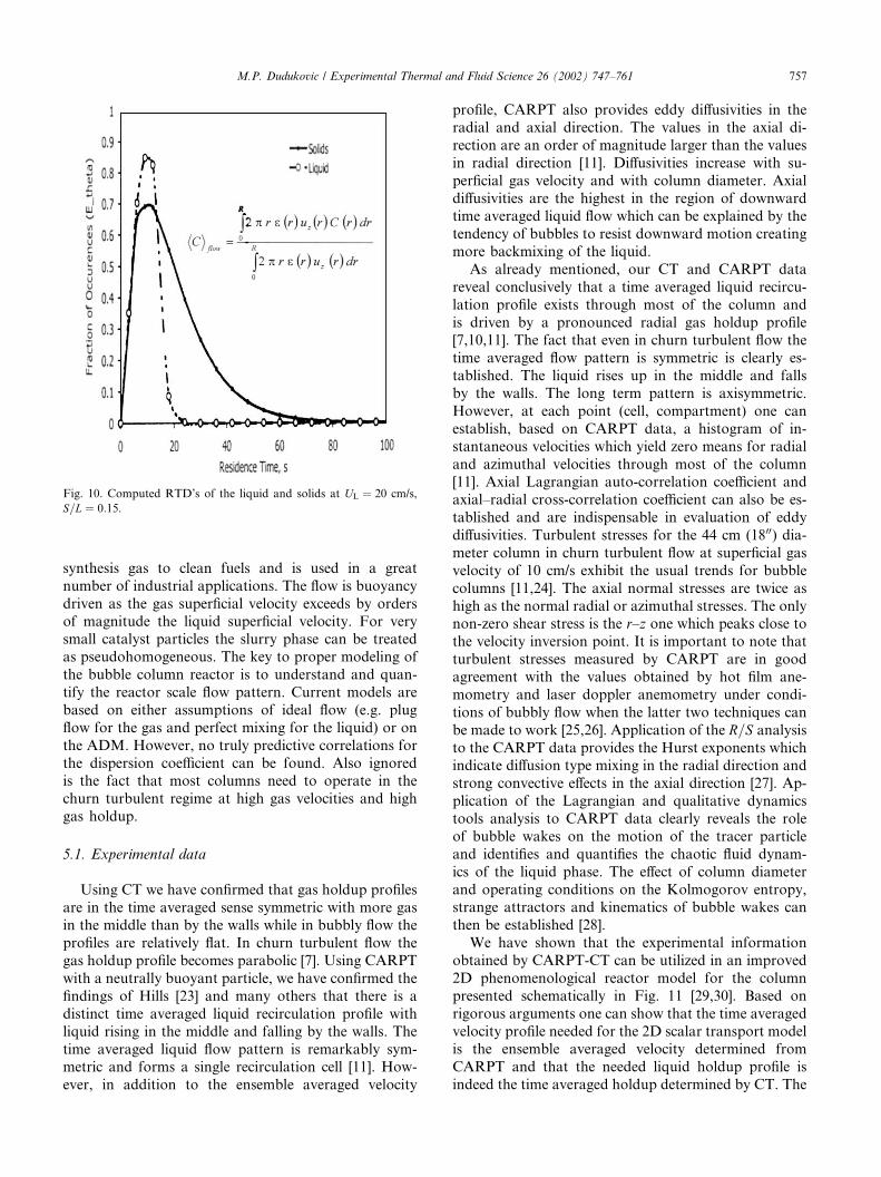
Computation was performed in the framework of theFluent two fluid model version 4. Both 2D axisymmetricand 3D simulations were performed. Best comparisonwith data was obtained with 3D simulations since theflow clearly has a 3D character. Such 3D simulationsusing 39,800 cells produce good agreement of calculatedtime averaged solids axial velocity profile and solidsholdup profile with CARPT and CT data as shown inFig. 9. Averaging is done from 25 to 100 s simulationtime. Granular temperature predictions are also goodexcept in the wall region. However the 3D simulationtook more than a month on a DEC Alpha 500 MHzmachine to execute. To provide faster input to reactormodeling, a 2D simulation coupled with a scalar tracertransport equation was executed and the results for theliquid and solids RTD are in agreement with experi-mental observation that liquid is close to plug flow andsolids are much more backmixed (Fig. 10). The differ-ences in the mean and variance between the computedand experimentally determined values are well within10%.

The following conclusions can be derived from thisstudy: the CARPT-CT technique provides the needed

information on solids holdup, velocity and mixing forestablishment of more accurate reactor models. Whileliquid in a liquid–solid riser is close to being in plug flow[14], solids are extensively backmixed. The Euler–Eulermodel is capable of computing reasonably well theoverall features of the reactor scale liquid and solidsflow via 2D axisymmetric simulation. The true transientnature of the flow is, however, only revealed by 3Dsimulations which produce results for time averagedvelocity, holdup and kinetic energy in good agreementwith experimental observations.

5. Bubble column flows

Let us now examine a bubble column, which is thereactor of choice for conversion of natural gas and

Fig. 9. Comparison of computed and measured values.


synthesis gas to clean fuels and is used in a greatnumber of industrial applications. The flow is buoyancydriven as the gas superficial velocity exceeds by ordersof magnitude the liquid superficial velocity. For verysmall catalyst particles the slurry phase can be treatedas pseudohomogeneous. The key to proper modeling ofthe bubble column reactor is to understand and quan-tify the reactor scale flow pattern. Current models arebased on either assumptions of ideal flow (e.g. plugflow for the gas and perfect mixing for the liquid) or onthe ADM. However, no truly predictive correlations forthe dispersion coefficient can be found. Also ignoredis the fact that most columns need to operate in thechurn turbulent regime at high gas velocities and highgas holdup.

5.1. Experimental data

Using CT we have confirmed that gas holdup profilesare in the time averaged sense symmetric with more gasin the middle than by the walls while in bubbly flow theprofiles are relatively flat. In churn turbulent flow thegas holdup profile becomes parabolic [7]. Using CARPTwith a neutrally buoyant particle, we have confirmed thefindings of Hills [23] and many others that there is adistinct time averaged liquid recirculation profile withliquid rising in the middle and falling by the walls. Thetime averaged liquid flow pattern is remarkably sym-metric and forms a single recirculation cell [11]. How-ever, in addition to the ensemble averaged velocity

profile, CARPT also provides eddy diffusivities in theradial and axial direction. The values in the axial di-rection are an order of magnitude larger than the valuesin radial direction [11]. Diffusivities increase with su-perficial gas velocity and with column diameter. Axialdiffusivities are the highest in the region of downwardtime averaged liquid flow which can be explained by thetendency of bubbles to resist downward motion creatingmore backmixing of the liquid.

As already mentioned, our CT and CARPT datareveal conclusively that a time averaged liquid recircu-lation profile exists through most of the column andis driven by a pronounced radial gas holdup profile[7,10,11]. The fact that even in churn turbulent flow thetime averaged flow pattern is symmetric is clearly es-tablished. The liquid rises up in the middle and fallsby the walls. The long term pattern is axisymmetric.However, at each point (cell, compartment) one canestablish, based on CARPT data, a histogram of in-stantaneous velocities which yield zero means for radialand azimuthal velocities through most of the column[11]. Axial Lagrangian auto-correlation coefficient andaxial–radial cross-correlation coefficient can also be es-tablished and are indispensable in evaluation of eddydiffusivities. Turbulent stresses for the 44 cm (1800) dia-meter column in churn turbulent flow at superficial gasvelocity of 10 cm/s exhibit the usual trends for bubblecolumns [11,24]. The axial normal stresses are twice ashigh as the normal radial or azimuthal stresses. The onlynon-zero shear stress is the r–z one which peaks close tothe velocity inversion point. It is important to note thatturbulent stresses measured by CARPT are in goodagreement with the values obtained by hot film ane-mometry and laser doppler anemometry under condi-tions of bubbly flow when the latter two techniques canbe made to work [25,26]. Application of the R=S analysisto the CARPT data provides the Hurst exponents whichindicate diffusion type mixing in the radial direction andstrong convective effects in the axial direction [27]. Ap-plication of the Lagrangian and qualitative dynamicstools analysis to CARPT data clearly reveals the roleof bubble wakes on the motion of the tracer particleand identifies and quantifies the chaotic fluid dynam-ics of the liquid phase. The effect of column diameterand operating conditions on the Kolmogorov entropy,strange attractors and kinematics of bubble wakes canthen be established [28].

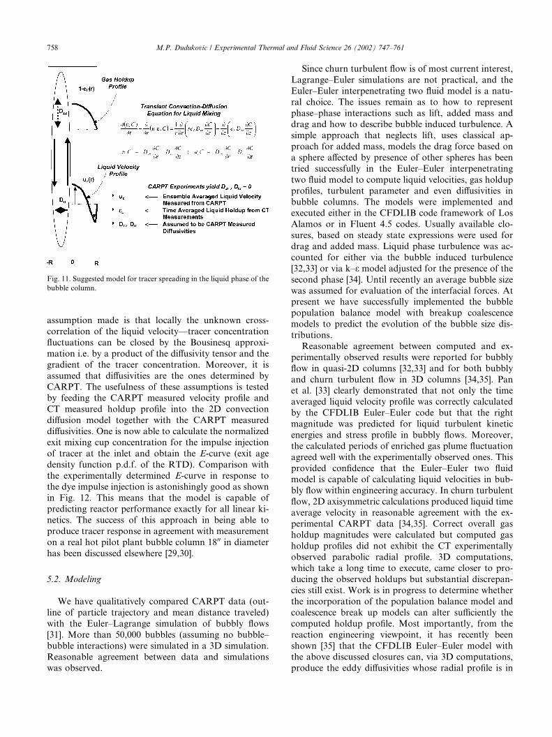
We have shown that the experimental informationobtained by CARPT-CT can be utilized in an improved2D phenomenological reactor model for the columnpresented schematically in Fig. 11 [29,30]. Based onrigorous arguments one can show that the time averagedvelocity profile needed for the 2D scalar transport modelis the ensemble averaged velocity determined fromCARPT and that the needed liquid holdup profile isindeed the time averaged holdup determined by CT. The

Fig. 10. Computed RTD’s of the liquid and solids at UL ¼ 20 cm/s,

S=L ¼ 0:15.


assumption made is that locally the unknown cross-correlation of the liquid velocity––tracer concentrationfluctuations can be closed by the Bousinesq approxi-mation i.e. by a product of the diffusivity tensor and thegradient of the tracer concentration. Moreover, it isassumed that diffusivities are the ones determined byCARPT. The usefulness of these assumptions is testedby feeding the CARPT measured velocity profile andCT measured holdup profile into the 2D convectiondiffusion model together with the CARPT measureddiffusivities. One is now able to calculate the normalizedexit mixing cup concentration for the impulse injectionof tracer at the inlet and obtain the E-curve (exit agedensity function p.d.f. of the RTD). Comparison withthe experimentally determined E-curve in response tothe dye impulse injection is astonishingly good as shownin Fig. 12. This means that the model is capable ofpredicting reactor performance exactly for all linear ki-netics. The success of this approach in being able toproduce tracer response in agreement with measurementon a real hot pilot plant bubble column 1800 in diameterhas been discussed elsewhere [29,30].

5.2. Modeling

We have qualitatively compared CARPT data (out-line of particle trajectory and mean distance traveled)with the Euler–Lagrange simulation of bubbly flows[31]. More than 50,000 bubbles (assuming no bubble–bubble interactions) were simulated in a 3D simulation.Reasonable agreement between data and simulationswas observed.

Since churn turbulent flow is of most current interest,Lagrange–Euler simulations are not practical, and theEuler–Euler interpenetrating two fluid model is a natu-ral choice. The issues remain as to how to representphase–phase interactions such as lift, added mass anddrag and how to describe bubble induced turbulence. Asimple approach that neglects lift, uses classical ap-proach for added mass, models the drag force based ona sphere affected by presence of other spheres has beentried successfully in the Euler–Euler interpenetratingtwo fluid model to compute liquid velocities, gas holdupprofiles, turbulent parameter and even diffusivities inbubble columns. The models were implemented andexecuted either in the CFDLIB code framework of LosAlamos or in Fluent 4.5 codes. Usually available clo-sures, based on steady state expressions were used fordrag and added mass. Liquid phase turbulence was ac-counted for either via the bubble induced turbulence[32,33] or via k–e model adjusted for the presence of thesecond phase [34]. Until recently an average bubble sizewas assumed for evaluation of the interfacial forces. Atpresent we have successfully implemented the bubblepopulation balance model with breakup coalescencemodels to predict the evolution of the bubble size dis-tributions.

Reasonable agreement between computed and ex-perimentally observed results were reported for bubblyflow in quasi-2D columns [32,33] and for both bubblyand churn turbulent flow in 3D columns [34,35]. Panet al. [33] clearly demonstrated that not only the timeaveraged liquid velocity profile was correctly calculatedby the CFDLIB Euler–Euler code but that the rightmagnitude was predicted for liquid turbulent kineticenergies and stress profile in bubbly flows. Moreover,the calculated periods of enriched gas plume fluctuationagreed well with the experimentally observed ones. Thisprovided confidence that the Euler–Euler two fluidmodel is capable of calculating liquid velocities in bub-bly flow within engineering accuracy. In churn turbulentflow, 2D axisymmetric calculations produced liquid timeaverage velocity in reasonable agreement with the ex-perimental CARPT data [34,35]. Correct overall gasholdup magnitudes were calculated but computed gasholdup profiles did not exhibit the CT experimentallyobserved parabolic radial profile. 3D computations,which take a long time to execute, came closer to pro-ducing the observed holdups but substantial discrepan-cies still exist. Work is in progress to determine whetherthe incorporation of the population balance model andcoalescence break up models can alter sufficiently thecomputed holdup profile. Most importantly, from thereaction engineering viewpoint, it has recently beenshown [35] that the CFDLIB Euler–Euler model withthe above discussed closures can, via 3D computations,produce the eddy diffusivities whose radial profile is in

Fig. 11. Suggested model for tracer spreading in the liquid phase of the

bubble column.


close agreement with values obtained from CARPT ex-periments. Hence, CFD offers possibilities in calculatingthe parameters needed for reactor modeling, such as timeaveraged velocity profile and eddy diffusivities. As men-tioned earlier a 2D convection–diffusion model thatutilizes CFD calculated flow parameters can be quiteuseful in predicting tracer responses and reactor perfor-mance of industrial size reactors.

6. Practical significance/usefulness

This paper describes the key features of and providesthe key references for CARPT-CT. The techniques areunique in their capabilities of providing the flow fielddescription in large enclosures for opaque systems. Theirutility in obtaining the solids holdup distribution, ve-locity and kinetic energy profiles in a liquid–solid riser

and in describing the liquid flow field in churn turbu-lent bubble columns is established. The capabilities ofthe Euler–Euler interpenetrating two fluid model ingenerating flow pattern information in agreement withCARPT-CT data that can form a basis for reactormodeling are also shown and are significant for indus-trial applications.

7. Concluding remarks

The CARPT-CT techniques provide us with the un-ique opportunities to assess holdup and velocity fields inopaque two phase systems. The resolutions of bothtechniques allow reliable information to be generatedfor large scale motion at lower frequencies. While CTprovides the time averaged density distribution, CARPT,in addition to time averaged velocities, allows estimation

Fig. 12. Prediction of non-volatile tracer impulse response.


of a number of turbulent quantities, e.g. kinetic energy,stresses, eddy diffusivities, etc.

The wealth of information provided by CARPT-CTallows us to quantify the flow fields in systems like liq-uid–solid risers and bubble columns which leads toimproved and more detailed reactor models. CFD com-putations, based on the Euler–Euler interpenetratingtwo fluid model have been shown to be capable ofproducing information in good agreement with data,which renders hope for CFD based scale-up in the fu-ture.

It is fair to conclude that CARPT-CT are indeed avaluable measurement tool for opaque multiphase sys-tems and that the Euler–Euler model has potential insimulation of reactor scale multiphase flows at condi-tions of industrial interest.

Acknowledgements

At the end I would like to thank the many collabo-rators that have produced all the results presented here.Above all, Narsi Devanathan, Yubo Yang and SaileshKumar deserve credit for designing, constructing andimplementing the hardware and software for CARPT-CT in CREL. Shantanu Roy and Abdenour Kemounexecuted the experiments in the liquid–solid riser dis-cussed here, and Shantanu modeled them using Fluentwith the help of Jay Sanyal (Fluent). Sue Degaleesan,Jinwen Chen, Booncheng Ong experimented with thebubble column, while Yu Pan and S. Roy solved CFDmodels with CFDLIB and Fluent. Muthanna Al-Dah-han offered helpful suggestions and Bernard Toseland ofAir Products was instrumental in focussing us to meetindustrial needs.

Finally, we are thankful to our financial sponsors:Exxon-Mobil for donating the CARPT-CT elements,Department of Energy and all CREL industrial sponsorcompanies from five continents (ABB Lummus, AirProducts, Bayer, Chevron, Conoco, Dow Chemicals,DuPont, Elf Atofina, ENI Technologies, Exxon-Mobil,IFP, Intevep, Mitsubishi, Praxair, Sasol, Shell, Solutia,Statoil, Synetix-ICI, UOP). Their financial supportmade this work possible.

References

[1] P.L. Mills, Recent development and advances in laboratory-scale

multiphase reactors, Plenary Lecture, First North American

Symposium on Chemical Reaction Engineering (NASCRE1),

Houston, TX, 2001.

[2] G.F. Froment, K.B. Bischoff, Chemical Reactor Analysis and

Design, second ed., Wiley, NY, 1990.

[3] J. Chaouki, F. Larachi, M.P. Dudukovic, Non-invasive tomo-

graphic and velocimetric monitoring of multiphase flows, Ind.

Eng. Chem. Res. 36 (11) (1997) 4476–4503.

[4] J. Chaouki, F. Larachi, M.P. Dudukovic (Eds.), Non-invasive

monitoring of multiphase flows, Elsevier, Amsterdam, 1997.

[5] S.B. Kumar, D. Moslemian, M.P. Dudukovic, A c-ray tomo-

graphic scanner for imaging of void distribution in two-phase flow

systems, Flow Meas. Instrum. 6 (3) (1995) 61–73.

[6] S.B. Kumar, M.P. Dudukovic, Computer assisted gamma and

x-ray tomography: Application to multiphase flow systems, in:

Chaouki et al. (Eds.), Non-Invasive Monitoring of Multiphase

Flows, Elsevier, Amsterdam, 1997, pp. 47–103, Chapter 2.

[7] S.B. Kumar, D. Moslemian, M.P. Dudukovic, Gas holdup

measurements in bubble columns using computed tomography,

AIChE J. 43 (6) (1997) 1414–1425.

[8] J.S. Lin, M.M. Chen, B.T. Chao, A novel radioactive particle

tracking facility for measurement of solids motion in gas fluidized

beds, AIChE J. 31 (3) (1985) 465–473.

[9] N. Devanathan, Investigation of liquid hydrodynamics in bubble

columns via computer-automated radioactive particle tracking

(CARPT), D.Sc. Thesis, Washington University, St. Louis, MO,

1991.

[10] N. Devanathan, D. Moslemian, M.P. Dudukovic, Flow mapping

in bubble columns using CARPT, Chem. Eng. Sci. 45 (8) (1990)

2285–2291.

[11] S. Degaleesan, Fluid dynamic measurements and modeling of

liquid mixing in bubble columns, D.Sc. Thesis, Washington

University, St. Louis, MO, 1997.

[12] F. Larachi, G. Kennedy, J. Chaouki, A c-ray detection system

for 3-D particle tracking in multiphase reactors, Nucl. Instrum.

Meth. A 338 (2-3) (1994) 568–576.

[13] P. Gupta, Bubble column dynamics: experiments and models,

D.Sc. Thesis, Washington University, St. Louis, MO, May, 2002.

[14] S. Roy, Quantification of two phase flows in liquid–solid risers,

D.Sc. Thesis, Washington University, St. Louis, MO, December,

2000.

[15] S. Roy, M.P. Dudukovic, Flow mapping and modeling of liquid-

solid risers, Ind. Eng. Chem. Res. 40 (23) (2001) 5440–5454.

[16] S. Roy, A. Kemoun, M. Al-Dahhan, M.P. Dudukovic, A method

for estimating the solids circulation rate in a closed-loop circu-

lating fluidized bed, Powder Technol. 121 (2–3) (2001) 213–222.

[17] D.A. Drew, Mathematical modeling of two phase flow, Ann. Rev.

Fluid Mech. 15 (1983) 261–291.

[18] S. Chapman, T.G. Cowling, Mathematical Theory and Nonuni-

form Gases, third ed., Cambridge University Press, Cambridge

UK, 1990.

[19] J. Ding, D. Gidaspow, A bubbling fluidization model using kinetic

theory of granular flow, AIChE J. 36 (4) (1990) 523–538.

[20] M.Y. Louge, E. Mastorakos, J.T. Jenkings, The role of particle

collisions on pneumatic transport, J. Fluid Mech. 231 (1991) 345–

359.

[21] C.Y. Wen, Y.H. Yu, Mechanics of fluidization, Chem. Eng.

Progr. Symp. Sci. 62 (62) (1966) 100–111.

[22] S.E. Elghobashi, T.W. Abou-Arab, A two-equation turbulence

model for two-phase flows, Phys. Fluids 26 (4) (1983) 931–938.

[23] J.H. Hills, Packed nonuniformity of velocity and voidage in a

bubble column, Trans. Inst. Chem. Eng. 52 (1974) 1–9.

[24] J. Chen, L. Fan, S. Degaleesan, P. Gupta, M.H. Al-Dahhan, M.P.

Dudukovic, B.A. Toseland, Fluid dynamic parameters in bubble

columns with internals, Chem. Eng. Sci. 54 (13/14) (1999) 2187–

2197.

[25] T. Menzel, T. Inderweide, O. Standacher, O. Wein, U. Onken,

Reynolds shear stress for modeling of bubble column reactors,

Ind. Eng. Chem. Res. 29 (6) (1990) 988–994.

[26] R.F. Mudde, J.S. Groen, H.E.A. van den Akker, Liquid velocity

field in bubble columns: LDA experiments, Chem. Eng. Sci. 52

(21/22) (1997) 4217–4224.

[27] Y.B. Yang, N. Devanathan, M.P. Dudukovic, Liquid backmixing

in bubble columns via computer-automated radioactive particle

tracking (CARPT), Exp. Fluids 16 (1) (1993) 1–9.


[28] M. Cassanello, F. Larachi, A. Kemoun, M. Al-Dahhan, M.P.

Dudukovic, Inferring liquid chaotic dynamics in bubble columns

using CARPT, Chem. Eng. Sci. 56 (21/22) (2002) 6125–6134.

[29] S. Degaleesan, S. Roy, S.B. Kumar, M.P. Dudukovic, Liquid

mixing based on convection and turbulent dispersion in bubble

columns, Chem. Eng. Sci. 51 (11) (1996) 2721–2725.

[30] S. Degaleesan, M.P. Dudukovic, B.A. Toseland, B.L. Bhatt, A

two compartment convective diffusion model for slurry bubble

column reactors, Ind. Eng. Chem. Res. 36 (11) (1997) 4670–4680.

[31] N. Devanathan, M.P. Dudukovic, A. Lapin, A. Lubbert, Chaotic

flow in bubble column reactors, Chem. Eng. Sci. 50 (16) (1995)

2661–2667.

[32] Y. Pan, M.P. Dudukovic, M. Chang, Dynamic simulation of

bubbly flow in bubble columns, Chem. Eng. Sci. 54 (13/14) (1999)

2481–2489.

[33] Y. Pan, M.P. Dudukovic, M. Chang, Numerical investigation of

gas driven flow in 2-D bubble columns, AIChE J. 46 (3) (2000)

434–449.

[34] J. Sanyal, S. Vasquez, S. Roy, M.P. Dudukovic, Numerical

simulation of gas–liquid dynamics in cylindrical bubble column

reactors, Chem. Eng. Sci. 55 (21) (1999) 5071–5083.

[35] Y. Pan, M.P. Dudukovic, CFD simulations of bubble columns,

6th World Congress of Chemical Engineering, Melbourne, Aus-

tralia, September, 2001.


opaque multiphase flows: experiments and modeling

Documents