online em algorithm and some extensions
TRANSCRIPT

Online EM Algorithm and Some Extensions
Olivier Cappe and Eric Moulines
Telecom ParisTech & CNRS
May 2011
O. Cappe and E. Moulines (@ Verona) Online EM Algorithm May 2011 1 / 35
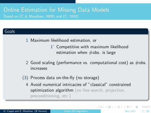
Online Estimation for Missing Data ModelsBased on (C & Moulines, 2009) and (C, 2010)
Goals
1 Maximum likelihood estimation, or
1’ Competitive with maximum likelihoodestimation when #obs. is large
2 Good scaling (performance vs. computational cost) as #obs.increases
(3) Process data on-the-fly (no storage)
4 Avoid numerical intricacies of ”classical” constrainedoptimization algorithm (no line-search, projection,preconditioning, etc.)
O. Cappe and E. Moulines (@ Verona) Online EM Algorithm May 2011 2 / 35

Outline
1 The EM Algorithm in Exponential Families
2 The Limiting EM Recursion
3 Online EM AlgorithmThe AlgorithmProperties and Discussion
4 Use for Batch ML Estimation
5 Extensions
6 References
O. Cappe and E. Moulines (@ Verona) Online EM Algorithm May 2011 3 / 35
The EM Algorithm in Exponential Families
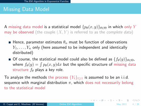
Missing Data Model
A missing data model is a statistical model {pθ(x, y)}θ∈Θ in which only Ymay be observed (the couple (X,Y ) is referred to as the complete data)
Hence, parameter estimates θn must be function of observationsY1, . . . , Yn only (here assumed to be independent and identicallydistributed)
Of course, the statistical model could also be defined as {fθ(y)}θ∈Θ,where fθ(y) =
∫pθ(x, y)dx but the specific structure of missing data
structure fθ plays a key role.
To analyze the methods the process {Yt}t≥1 is assumed to be an i.i.d.sequence with marginal distribution π, which does not necessarily belongto the statistical model
O. Cappe and E. Moulines (@ Verona) Online EM Algorithm May 2011 4 / 35

The EM Algorithm in Exponential Families
Finite Mixture Model
Mixture probability density function
f(y) =
m∑i=1
αifi(y)
Missing Data Interpretation
P(Xt = i) = αi
Yt|Xt = i ∼ fi(y)
O. Cappe and E. Moulines (@ Verona) Online EM Algorithm May 2011 5 / 35
The EM Algorithm in Exponential Families
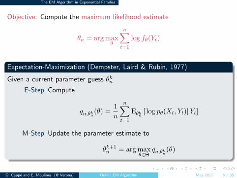
Objective: Compute the maximum likelihood estimate
θn = arg maxθ
n∑t=1
log fθ(Yt)
Expectation-Maximization (Dempster, Laird & Rubin, 1977)
Given a current parameter guess θkn
E-Step Compute
qn,θkn(θ) =1
n
n∑t=1
Eθkn [ log pθ(Xt, Yt)|Yt]
M-Step Update the parameter estimate to
θk+1n = arg max
θ∈Θqn,θkn(θ)
O. Cappe and E. Moulines (@ Verona) Online EM Algorithm May 2011 6 / 35
The EM Algorithm in Exponential Families
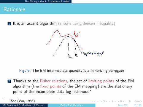
Rationale
1 It is an ascent algorithm (shown using Jensen inequality)
Figure: The EM intermediate quantity is a minorizing surrogate
2 Thanks to the Fisher relations, the set of limiting points of the EMalgorithm (the fixed points of the EM mapping) are the stationarypoint of the incomplete data log-likelihood∗
∗See (Wu, 1983)O. Cappe and E. Moulines (@ Verona) Online EM Algorithm May 2011 7 / 35
The EM Algorithm in Exponential Families
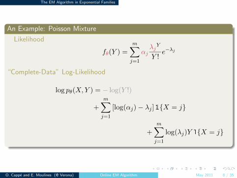
An Example: Poisson Mixture
Likelihood
fθ(Y ) =
m∑j=1
αjλjY
Y !e−λj
“Complete-Data” Log-Likelihood
log pθ(X,Y ) = − log(Y !)
+
m∑j=1
[log(αj)− λj ]1{X = j}
+
m∑j=1
log(λj)Y 1{X = j}
O. Cappe and E. Moulines (@ Verona) Online EM Algorithm May 2011 8 / 35
The EM Algorithm in Exponential Families
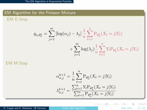
EM Algorithm for the Poisson Mixture
EM E-Step
qn,θkn =
m∑j=1
[log(αj)− λj ]1
n
n∑t=1
Pθkn(Xt = j|Yt)
+
m∑j=1
log(λj)1
n
n∑t=1
YtPθkn(Xt = j|Yt)
EM M-Step
αk+1n,j =
1
n
n∑t=1
Pθkn(Xt = j|Yt)
λk+1n,j =
∑nt=1 YtPθkn(Xt = j|Yt)∑nt=1 Pθkn(Xt = j|Yt)
O. Cappe and E. Moulines (@ Verona) Online EM Algorithm May 2011 9 / 35
The EM Algorithm in Exponential Families
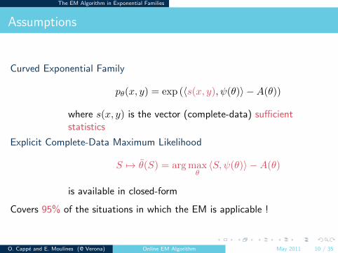
Assumptions
Curved Exponential Family
pθ(x, y) = exp (〈s(x, y), ψ(θ)〉 −A(θ))
where s(x, y) is the vector (complete-data) sufficientstatistics
Explicit Complete-Data Maximum Likelihood
S 7→ θ(S) = arg maxθ〈S, ψ(θ)〉 −A(θ)
is available in closed-form
Covers 95% of the situations in which the EM is applicable !
O. Cappe and E. Moulines (@ Verona) Online EM Algorithm May 2011 10 / 35
The EM Algorithm in Exponential Families
The EM Algorithm Revisited
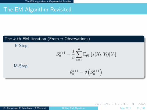
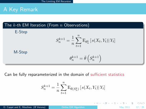
The k-th EM Iteration (From n Observations)
E-Step
Sk+1n =
1
n
n∑t=1
Eθkn [s(Xt, Yt)|Yt]
M-Step
θk+1n = θ
(Sk+1n
)
O. Cappe and E. Moulines (@ Verona) Online EM Algorithm May 2011 11 / 35
The Limiting EM Recursion
A Key Remark
The k-th EM Iteration (From n Observations)
E-Step
Sk+1n =
1
n
n∑t=1
Eθkn [s(Xt, Yt)|Yt]
M-Step
θk+1n = θ
(Sk+1n
)
Can be fully reparameterized in the domain of sufficient statistics
Sk+1n =
1
n
n∑t=1
Eθ(Skn) [s(Xt, Yt)|Yt]
O. Cappe and E. Moulines (@ Verona) Online EM Algorithm May 2011 12 / 35
The Limiting EM Recursion
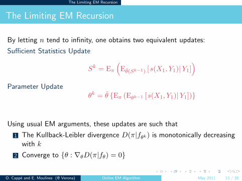
The Limiting EM Recursion
By letting n tend to infinity, one obtains two equivalent updates:
Sufficient Statistics Update
Sk = Eπ
(Eθ(Sk−1) [s(X1, Y1)|Y1]
)Parameter Update
θk = θ {Eπ (Eθk−1 [s(X1, Y1)|Y1])}
Using usual EM arguments, these updates are such that
1 The Kullback-Leibler divergence D(π|fθk) is monotonically decreasingwith k
2 Converge to {θ : ∇θD(π|fθ) = 0}
O. Cappe and E. Moulines (@ Verona) Online EM Algorithm May 2011 13 / 35
The Limiting EM Recursion
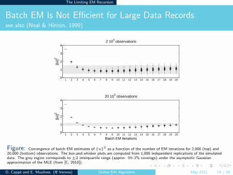
Batch EM Is Not Efficient for Large Data Recordssee also (Neal & Hinton, 1999)
0
1
2
3
4
1 2 3 4 5 6 7 8 9 10 11 12 13 14 15 16 17 18 19 20
Batch EM iterations
||u||2
20 103 observations
0
1
2
3
4
1 2 3 4 5 6 7 8 9 10 11 12 13 14 15 16 17 18 19 20
||u||2
2 103 observations
Figure: Convergence of batch EM estimates of ‖u‖2 as a function of the number of EM iterations for 2,000 (top) and20,000 (bottom) observations. The box-and-whisker plots are computed from 1,000 independent replications of the simulateddata. The grey region corresponds to ±2 interquartile range (approx. 99.3% coverage) under the asymptotic Gaussianapproximation of the MLE (from [C, 2010]).
O. Cappe and E. Moulines (@ Verona) Online EM Algorithm May 2011 14 / 35
Online EM Algorithm The Algorithm
The Online EM Algorithm
The online EM algorithm outputs one updated parameter estimate θnafter processing each individual observation Yn
The parameter update is very similar to applying the EM algorithm tothe single observation Yn (with smoothing)
The memory footprint of the algorithm is constant while itscomputational cost is proportional to the number of processedobservations
O. Cappe and E. Moulines (@ Verona) Online EM Algorithm May 2011 15 / 35
Online EM Algorithm The Algorithm
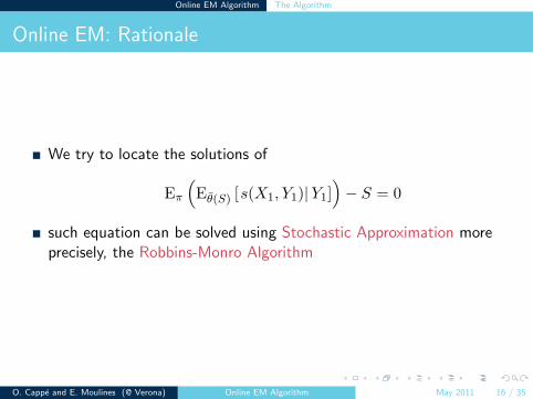
Online EM: Rationale
We try to locate the solutions of
Eπ
(Eθ(S) [s(X1, Y1)|Y1]
)− S = 0
such equation can be solved using Stochastic Approximation moreprecisely, the Robbins-Monro Algorithm
O. Cappe and E. Moulines (@ Verona) Online EM Algorithm May 2011 16 / 35
Online EM Algorithm The Algorithm
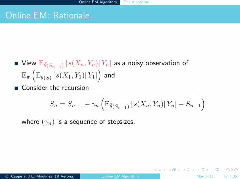
Online EM: Rationale
View Eθ(Sn−1) [s(Xn, Yn)|Yn] as a noisy observation of
Eπ
(Eθ(S) [s(X1, Y1)|Y1]
)and
Consider the recursion
Sn = Sn−1 + γn
(Eθ(Sn−1) [s(Xn, Yn)|Yn]− Sn−1
)where (γn) is a sequence of stepsizes.
O. Cappe and E. Moulines (@ Verona) Online EM Algorithm May 2011 17 / 35
Online EM Algorithm The Algorithm
The Algorithm
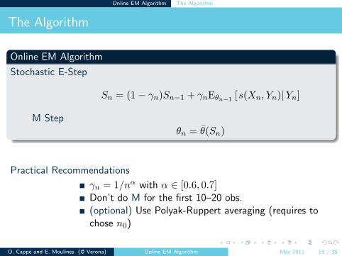
Online EM Algorithm
Stochastic E-Step
Sn = (1− γn)Sn−1 + γnEθn−1 [s(Xn, Yn)|Yn]
M Stepθn = θ(Sn)
Practical Recommendations
γn = 1/nα with α ∈ [0.6, 0.7]Don’t do M for the first 10–20 obs.(optional) Use Polyak-Ruppert averaging (requires tochose n0)
O. Cappe and E. Moulines (@ Verona) Online EM Algorithm May 2011 18 / 35
Online EM Algorithm The Algorithm
Online EM in the Poisson Mixture Example
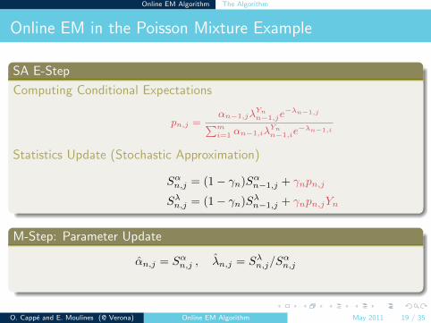
SA E-Step
Computing Conditional Expectations
pn,j =αn−1,jλ
Ynn−1,je
−λn−1,j∑mi=1 αn−1,iλ
Ynn−1,ie
−λn−1,i
Statistics Update (Stochastic Approximation)
Sαn,j = (1− γn)Sαn−1,j + γnpn,j
Sλn,j = (1− γn)Sλn−1,j + γnpn,jYn
M-Step: Parameter Update
αn,j = Sαn,j , λn,j = Sλn,j/Sαn,j
O. Cappe and E. Moulines (@ Verona) Online EM Algorithm May 2011 19 / 35
Online EM Algorithm Properties and Discussion
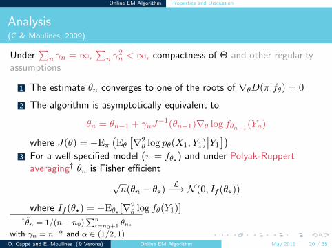
Analysis(C & Moulines, 2009)
Under∑
n γn =∞,∑
n γ2n <∞, compactness of Θ and other regularity
assumptions
1 The estimate θn converges to one of the roots of ∇θD(π|fθ) = 0
2 The algorithm is asymptotically equivalent to
θn = θn−1 + γnJ−1(θn−1)∇θ log fθn−1(Yn)
where J(θ) = −Eπ(Eθ[∇2θ log pθ(X1, Y1)
∣∣Y1
])3 For a well specified model (π = fθ?) and under Polyak-Ruppert
averaging† θn is Fisher efficient
√n(θn − θ?)
L−→ N (0, If (θ?))
where If (θ?) = −Eθ? [∇2θ log fθ(Y1)]
†θn = 1/(n− n0)∑nt=n0+1 θn,
with γn = n−α and α ∈ (1/2, 1)O. Cappe and E. Moulines (@ Verona) Online EM Algorithm May 2011 20 / 35
Online EM Algorithm Properties and Discussion
Some More Details
1 (Andrieu et al., 2005) but also (Delyon, 1994), (Benaım, 1999) usingthe fact that D(π|fθ(S)) is a Lyapunov function:⟨
∇SD(π|fθ(S)) , Eπ
(Eθ(S) [s(X1, Y1)|Y1]
)− S︸ ︷︷ ︸
mean field
⟩≤ 0
2 Taylor series expansion of θ to establish the equivalence (withremainder a.s. o(γn))
3 (Pelletier, 1998) to show that
γ−1/2n (θn − θ?)L−→ N (0, I−1p (θ?)/2)
in well-specified models (where Ip is the complete-data Fisherinformation matrix)General results of (Polyak and Judistky, 1992), (Mokkadem andPelletier, 2006) on averaging
O. Cappe and E. Moulines (@ Verona) Online EM Algorithm May 2011 21 / 35
Online EM Algorithm Properties and Discussion
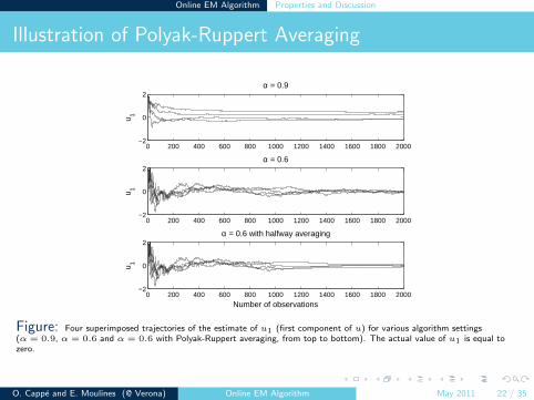
Illustration of Polyak-Ruppert Averaging
0 200 400 600 800 1000 1200 1400 1600 1800 2000−2
0
2
u 1
Number of observations
α = 0.6 with halfway averaging
0 200 400 600 800 1000 1200 1400 1600 1800 2000−2
0
2
u 1
α = 0.6
0 200 400 600 800 1000 1200 1400 1600 1800 2000−2
0
2
u 1
α = 0.9
Figure: Four superimposed trajectories of the estimate of u1 (first component of u) for various algorithm settings(α = 0.9, α = 0.6 and α = 0.6 with Polyak-Ruppert averaging, from top to bottom). The actual value of u1 is equal tozero.
O. Cappe and E. Moulines (@ Verona) Online EM Algorithm May 2011 22 / 35
Online EM Algorithm Properties and Discussion
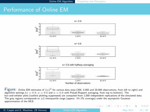
Performance of Online EM
0
1
2
3
4
0.2 10^3 2 10^3 20 10^3
Number of observations
||u||2
α = 0.6 with halfway averaging
01234
0.2 10^3 2 10^3 20 10^3
||u||2
α = 0.6
01234
0.2 10^3 2 10^3 20 10^3||u
||2
α = 0.9
Figure: Online EM estimates of ‖u‖2 for various data sizes (200, 2,000 and 20,000 observations, from left to right) andalgorithm settings (α = 0.9, α = 0.6 and α = 0.6 with Polyak-Ruppert averaging, from top to bottom). Thebox-and-whisker plots (outliers plotting suppressed) are computed from 1,000 independent replications of the simulated data.The grey regions corresponds to ±2 interquartile range (approx. 99.3% coverage) under the asymptotic Gaussianapproximation of the MLE.
O. Cappe and E. Moulines (@ Verona) Online EM Algorithm May 2011 23 / 35
Online EM Algorithm Properties and Discussion
Related Works
(Titterington, 1984) Proposes a gradient algorithm
θn = θn−1 + γnI−1p (θn−1)∇θ log fθn−1(Yn)
It is asymptotically equivalent to the algorithm (previouslydescribed) for well-specified models (π = fθ?)
(Neal & Hinton, 1999) Describe an algorithm called Incremental EM thatis equivalent (up to first batch scan only) to Online EM usedwith γn = 1/n
(Sato, 2000; Sato & Ishii, 2000) Describe the algorithm and provide someanalysis in the flat model case and for mixtures of Gaussian
O. Cappe and E. Moulines (@ Verona) Online EM Algorithm May 2011 24 / 35
Online EM Algorithm Properties and Discussion
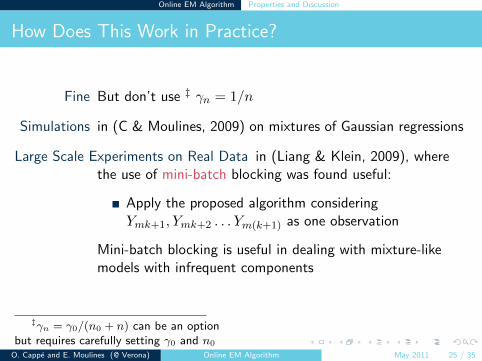
How Does This Work in Practice?
Fine But don’t use ‡ γn = 1/n
Simulations in (C & Moulines, 2009) on mixtures of Gaussian regressions
Large Scale Experiments on Real Data in (Liang & Klein, 2009), wherethe use of mini-batch blocking was found useful:
Apply the proposed algorithm consideringYmk+1, Ymk+2 . . . Ym(k+1) as one observation
Mini-batch blocking is useful in dealing with mixture-likemodels with infrequent components
‡γn = γ0/(n0 + n) can be an optionbut requires carefully setting γ0 and n0
O. Cappe and E. Moulines (@ Verona) Online EM Algorithm May 2011 25 / 35
Online EM Algorithm Properties and Discussion
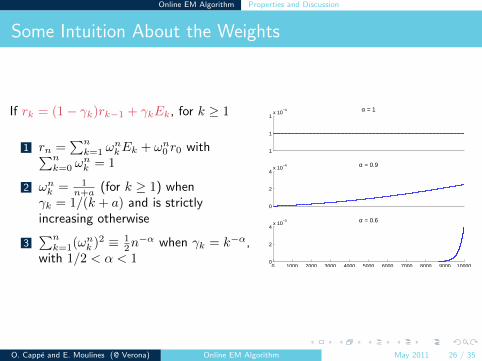
Some Intuition About the Weights
If rk = (1− γk)rk−1 + γkEk, for k ≥ 1
1 rn =∑nk=1 ω
nkEk + ωn0 r0 with∑n
k=0 ωnk = 1
2 ωnk = 1n+a (for k ≥ 1) when
γk = 1/(k + a) and is strictlyincreasing otherwise
3∑nk=1(ωnk )2 ≡ 1
2n−α when γk = k−α,
with 1/2 < α < 10 1000 2000 3000 4000 5000 6000 7000 8000 9000 10000
0
2
4x 10
−3 α = 0.6
0
2
4x 10
−4 α = 0.9
1
1
1x 10
−4 α = 1
O. Cappe and E. Moulines (@ Verona) Online EM Algorithm May 2011 26 / 35
Use for Batch ML Estimation
How to Use Online EM for Batch ML Estimation?
The most popular use of the method is to perfom batch ML estimationfrom very large datasets
Because we did not assume that π = fθ? , the previous analysis can beapplied to π ≡ the empirical measure associated with Y1, . . . , Yn
Online EM can be used for batch ML estimation by (randomly)scanning the data Y1, . . . , Yn
Convergence “speed” (with averaging) is (nobs. × nscans)−1/2 versus
ρnscans for batch EM
Not a fair comparison in terms of computing time as the M-Step isnot free and possible parallelization is ignored
O. Cappe and E. Moulines (@ Verona) Online EM Algorithm May 2011 27 / 35
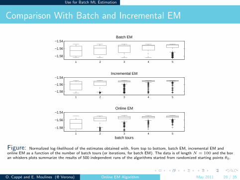
Use for Batch ML Estimation
Comparison With Batch and Incremental EM
−1.58
−1.56
−1.54
1 2 3 4 5
batch tours
Online EM
−1.58
−1.56
−1.54
1 2 3 4 5
Incremental EM
−1.58
−1.56
−1.54
1 2 3 4 5
Batch EM
Figure: Normalized log-likelihood of the estimates obtained with, from top to bottom, batch EM, incremental EM andonline EM as a function of the number of batch tours (or iterations, for batch EM). The data is of length N = 100 and the boxan whiskers plots summarize the results of 500 independent runs of the algorithms started from randomized starting points θ0.
O. Cappe and E. Moulines (@ Verona) Online EM Algorithm May 2011 28 / 35
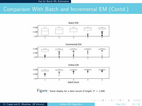
Use for Batch ML Estimation
Comparison With Batch and Incremental EM (Contd.)
−1.6
−1.58
−1.56
1 2 3 4 5
batch tours
Online EM
−1.6
−1.58
−1.56
1 2 3 4 5
Incremental EM
−1.6
−1.58
−1.56
1 2 3 4 5
Batch EM
Figure: Same display for a data record of length N = 1,000.
O. Cappe and E. Moulines (@ Verona) Online EM Algorithm May 2011 29 / 35
Extensions
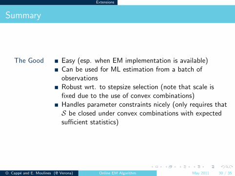
Summary
The Good Easy (esp. when EM implementation is available)Can be used for ML estimation from a batch ofobservationsRobust wrt. to stepsize selection (note that scale isfixed due to the use of convex combinations)Handles parameter constraints nicely (only requires thatS be closed under convex combinations with expectedsufficient statistics)
O. Cappe and E. Moulines (@ Verona) Online EM Algorithm May 2011 30 / 35
Extensions
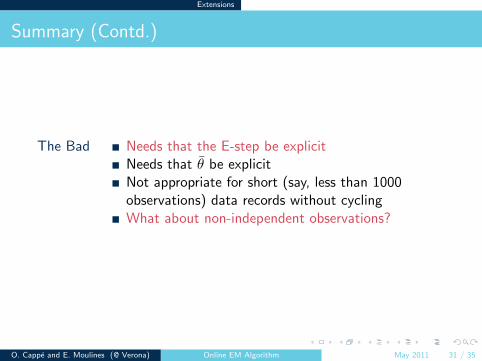
Summary (Contd.)
The Bad Needs that the E-step be explicitNeeds that θ be explicitNot appropriate for short (say, less than 1000observations) data records without cyclingWhat about non-independent observations?
O. Cappe and E. Moulines (@ Verona) Online EM Algorithm May 2011 31 / 35
Extensions
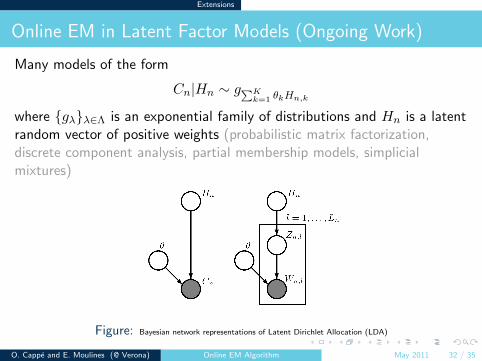
Online EM in Latent Factor Models (Ongoing Work)
Many models of the form
Cn|Hn ∼ g∑Kk=1 θkHn,k
where {gλ}λ∈Λ is an exponential family of distributions and Hn is a latentrandom vector of positive weights (probabilistic matrix factorization,discrete component analysis, partial membership models, simplicialmixtures)
Figure: Bayesian network representations of Latent Dirichlet Allocation (LDA)
O. Cappe and E. Moulines (@ Verona) Online EM Algorithm May 2011 32 / 35
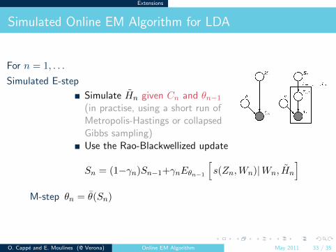
Extensions
Simulated Online EM Algorithm for LDA
For n = 1, . . .
Simulated E-step
Simulate Hn given Cn and θn−1
(in practise, using a short run ofMetropolis-Hastings or collapsedGibbs sampling)Use the Rao-Blackwellized update
Sn = (1−γn)Sn−1+γnEθn−1
[s(Zn,Wn)|Wn, Hn
]M-step θn = θ(Sn)
O. Cappe and E. Moulines (@ Verona) Online EM Algorithm May 2011 33 / 35
Extensions
Ignoring the sampling bias, this recursion can be analyzed and has thesame asymptotic properties as the online EM algorithm
In particular, for well-specified models,
γ−1/2n (θn − θ?)
L−→ N (0, I−1f (θ?))
instead ofγ−1/2n (θn − θ?)
L−→ N (0, I−1p (θ?))
for the “exact” online EM algorithm (Ip(θ?) = −Eθ? [∇2θ log pθ(X1, Y1)]).
O. Cappe and E. Moulines (@ Verona) Online EM Algorithm May 2011 34 / 35

References
Cappe, O. & Moulines, E. (2009). On-line expectation-maximization algorithm forlatent data models. J. Roy. Statist. Soc. B, 71(3):593-613.
Cappe, O. (2011). Online Expectation-Maximisation. To appear in Mengersen, K.,Titterington, M., & Robert, C. P., eds., Mixtures, Wiley.
Liang, P. & Klein, D. (2009). Online EM for Unsupervised Models. In ProcNAACL Conference.
Neal, R. M. & Hinton, G. E. (1999). A view of the EM algorithm that justifiesincremental, sparse, and other variants. In Jordan, M. I., ed., Learning in graphicalmodels, pages 355–368. MIT Press, Cambridge, MA, USA.
Rohde, D. & Cappe, O. (2011). Online maximum-likelihood estimation for latentfactor models. Submitted.
Sato, M. (2000). Convergence of on-line EM algorithm. In Proc. InternationalConference on Neural Information Processing, 1:476–481.
Sato, M. & Ishii, S. (2000). On-line EM algorithm for the normalized Gaussiannetwork. Neural Computation, 12:407-432.
Titterington, D. M. (1984). Recursive parameter estimation using incompletedata. J. Roy. Statist. Soc. B, 46(2):257-267.
O. Cappe and E. Moulines (@ Verona) Online EM Algorithm May 2011 35 / 35